Download Manual for SIENA version 3.2. - the Department of Statistics

Manual for SIENA version 3
Tom A.B. Snijders
Christian E.G. Steglich
Michael Schweinberger
Mark Huisman
University of Groningen: ICS, Department of Sociology
Grote Rozenstraat 31, 9712 TG Groningen, The Netherlands
University of Oxford: Department of Statistics
April 16, 2007
Abstract
SIENA (for Simulation Investigation for Empirical Network Analysis) is a computer program that
carries out the statistical estimation of models for the evolution of social networks according
to the dynamic actor-oriented model of Snijders (2001, 2005) and Snijders, Steglich, and
Schweinberger (2007). It also carries out MCMC estimation for the exponential random graph
model according to the procedures described in Snijders (2002) and Snijders, Pattison, Robins,
and Handcock (2006).
1
Contents
1 General information
5
I
7
Minimal Intro
2 General remarks for StOCNET.
2.1 Operating StOCNET. . . . . . . . . . . . . . . . . . . . . . . . . . . . . . . . . . . . . . . . .
7
7
3 Using SIENA
3.1 Steps for estimation: Choosing SIENA in StOCNET. . . . . . . . . . . . . . . . . . . . . . .
3.2 Steps for looking at results: Executing SIENA. . . . . . . . . . . . . . . . . . . . . . . . . . .
3.3 Giving references . . . . . . . . . . . . . . . . . . . . . . . . . . . . . . . . . . . . . . . . . .
8
8
9
10
II
User’s manual
11
4 Program parts
5 Input data
5.1 Digraph data files . . . . . . . . . . . . . .
5.1.1 Structurally determined values . .
5.2 Dyadic covariates . . . . . . . . . . . . . .
5.3 Individual covariates . . . . . . . . . . . .
5.4 Interactions and dyadic transformations of
5.5 Dependent action variables . . . . . . . .
5.6 Missing data . . . . . . . . . . . . . . . .
5.7 Composition change . . . . . . . . . . . .
5.8 Centering . . . . . . . . . . . . . . . . . .
11
.
.
.
.
.
.
.
.
.
.
.
.
.
.
.
.
.
.
.
.
.
.
.
.
.
.
.
.
.
.
.
.
.
.
.
.
.
.
.
.
.
.
.
.
.
.
.
.
.
.
.
.
.
.
.
.
.
.
.
.
.
.
.
.
.
.
.
.
.
.
.
.
.
.
.
.
.
.
.
.
.
.
.
.
.
.
.
.
.
.
.
.
.
.
.
.
.
.
.
.
.
.
.
.
.
.
.
.
.
.
.
.
.
.
.
.
.
.
.
.
.
.
.
.
.
.
.
.
.
.
.
.
.
.
.
.
.
.
.
.
.
.
.
.
.
.
.
.
.
.
.
.
.
.
.
.
.
.
.
.
.
.
.
.
.
.
.
.
.
.
.
.
.
.
.
.
.
.
.
.
.
.
.
.
.
.
.
.
.
12
12
13
14
14
15
15
16
16
18
6 Model specification
6.1 Important structural effects for network dynamics . . .
6.2 Effects for network dynamics associated with covariates
6.3 Effects on behavior evolution . . . . . . . . . . . . . . .
6.4 Exponential Random Graph Models . . . . . . . . . . .
6.5 Model Type . . . . . . . . . . . . . . . . . . . . . . . . .
6.5.1 Model Type: directed networks . . . . . . . . . .
6.5.2 Model Type: non-directed networks . . . . . . .
6.6 Additional interaction effects . . . . . . . . . . . . . . .
.
.
.
.
.
.
.
.
.
.
.
.
.
.
.
.
.
.
.
.
.
.
.
.
.
.
.
.
.
.
.
.
.
.
.
.
.
.
.
.
.
.
.
.
.
.
.
.
.
.
.
.
.
.
.
.
.
.
.
.
.
.
.
.
.
.
.
.
.
.
.
.
.
.
.
.
.
.
.
.
.
.
.
.
.
.
.
.
.
.
.
.
.
.
.
.
.
.
.
.
.
.
.
.
.
.
.
.
.
.
.
.
.
.
.
.
.
.
.
.
.
.
.
.
.
.
.
.
.
.
.
.
.
.
.
.
.
.
.
.
.
.
.
.
.
.
.
.
.
.
.
.
.
.
.
.
.
.
.
.
19
20
21
22
23
23
23
24
25
7 Estimation
7.1 Algorithm . . . . . . . . . . . . . . . . . . . . . . . . . . . . . . . . . . .
7.2 Output . . . . . . . . . . . . . . . . . . . . . . . . . . . . . . . . . . . .
7.3 Other remarks about the estimation algorithm . . . . . . . . . . . . . .
7.3.1 Changing initial parameter values for estimation . . . . . . . . .
7.3.2 Fixing parameters . . . . . . . . . . . . . . . . . . . . . . . . . .
7.3.3 Automatic fixing of parameters . . . . . . . . . . . . . . . . . . .
7.3.4 Conditional and unconditional estimation . . . . . . . . . . . . .
7.3.5 Automatic changes from conditional to unconditional estimation
.
.
.
.
.
.
.
.
.
.
.
.
.
.
.
.
.
.
.
.
.
.
.
.
.
.
.
.
.
.
.
.
.
.
.
.
.
.
.
.
.
.
.
.
.
.
.
.
.
.
.
.
.
.
.
.
.
.
.
.
.
.
.
.
.
.
.
.
.
.
.
.
.
.
.
.
.
.
.
.
.
.
.
.
.
.
.
.
27
27
28
31
31
31
31
31
32
. . . . . .
. . . . . .
. . . . . .
. . . . . .
covariates
. . . . . .
. . . . . .
. . . . . .
. . . . . .
8 Standard errors
.
.
.
.
.
.
.
.
.
32
2
9 Tests
9.1 Goodness of fit testing . . . . . . . . . . . . . . . . . . . . . . . .
9.2 How-to-do . . . . . . . . . . . . . . . . . . . . . . . . . . . . . . .
9.3 Example: one-sided tests, two-sided tests, and one-step estimates
9.3.1 Multi-parameter tests . . . . . . . . . . . . . . . . . . . .
9.3.2 Testing homogeneity assumptions . . . . . . . . . . . . . .
9.4 Alternative application: convergence problems . . . . . . . . . . .
.
.
.
.
.
.
.
.
.
.
.
.
.
.
.
.
.
.
.
.
.
.
.
.
.
.
.
.
.
.
.
.
.
.
.
.
.
.
.
.
.
.
.
.
.
.
.
.
.
.
.
.
.
.
.
.
.
.
.
.
.
.
.
.
.
.
.
.
.
.
.
.
.
.
.
.
.
.
.
.
.
.
.
.
.
.
.
.
.
.
33
33
33
34
35
36
36
10 Simulation
37
10.1 Conditional and unconditional simulation . . . . . . . . . . . . . . . . . . . . . . . . . . . . 37
11 Exponential random graphs
38
12 Options for model type, estimation and simulation
40
13 Getting started
13.1 Model choice . . . . . . . . . . .
13.1.1 Exploring which effects to
13.2 Convergence problems . . . . . .
13.3 Composition change . . . . . . .
. . . . .
include
. . . . .
. . . . .
.
.
.
.
.
.
.
.
.
.
.
.
.
.
.
.
.
.
.
.
.
.
.
.
.
.
.
.
.
.
.
.
.
.
.
.
.
.
.
.
.
.
.
.
.
.
.
.
.
.
.
.
.
.
.
.
.
.
.
.
.
.
.
.
.
.
.
.
.
.
.
.
.
.
.
.
.
.
.
.
.
.
.
.
.
.
.
.
.
.
.
.
.
.
.
.
.
.
.
.
.
.
.
.
.
.
.
.
.
.
.
.
14 Multilevel network analysis
42
42
43
43
44
46
15 Formulas for effects
15.1 Network evolution . . . . . . . . . . . . . . . .
15.1.1 Network evaluation function . . . . . . .
15.1.2 Network endowment function . . . . . .
15.1.3 Network rate function . . . . . . . . . .
15.1.4 Network rate function for Model Type 2
15.2 Behavioral evolution . . . . . . . . . . . . . . .
15.2.1 Behavioral evaluation function . . . . .
15.2.2 Behavioral endowment function . . . . .
15.2.3 Behavioral rate function . . . . . . . . .
15.3 Exponential random graph model . . . . . . . .
.
.
.
.
.
.
.
.
.
.
.
.
.
.
.
.
.
.
.
.
.
.
.
.
.
.
.
.
.
.
.
.
.
.
.
.
.
.
.
.
.
.
.
.
.
.
.
.
.
.
.
.
.
.
.
.
.
.
.
.
.
.
.
.
.
.
.
.
.
.
.
.
.
.
.
.
.
.
.
.
.
.
.
.
.
.
.
.
.
.
.
.
.
.
.
.
.
.
.
.
.
.
.
.
.
.
.
.
.
.
.
.
.
.
.
.
.
.
.
.
.
.
.
.
.
.
.
.
.
.
.
.
.
.
.
.
.
.
.
.
.
.
.
.
.
.
.
.
.
.
.
.
.
.
.
.
.
.
.
.
.
.
.
.
.
.
.
.
.
.
.
.
.
.
.
.
.
.
.
.
.
.
.
.
.
.
.
.
.
.
.
.
.
.
.
.
.
.
.
.
.
.
.
.
.
.
.
.
.
.
.
.
.
.
.
.
.
.
.
.
.
.
.
.
.
.
.
.
.
.
.
.
.
.
.
.
.
.
.
.
.
.
.
.
.
.
.
.
.
.
47
47
47
50
50
51
52
52
54
54
54
16 Running Siena outside of StOCNET
57
17 Limitations and time use
59
18 Changes compared to earlier versions
59
3
III
Programmer’s manual
62
19 SIENA files
19.1 Basic information file . . . . . . . . . . . . . . . .
19.2 Definition files . . . . . . . . . . . . . . . . . . .
19.2.1 Model specification through the MO file .
19.2.2 Specification of simulations through the SI
19.3 Data files . . . . . . . . . . . . . . . . . . . . . .
19.4 Output files . . . . . . . . . . . . . . . . . . . . .
. . .
. . .
. . .
file .
. . .
. . .
.
.
.
.
.
.
.
.
.
.
.
.
.
.
.
.
.
.
.
.
.
.
.
.
.
.
.
.
.
.
.
.
.
.
.
.
.
.
.
.
.
.
.
.
.
.
.
.
.
.
.
.
.
.
.
.
.
.
.
.
.
.
.
.
.
.
.
.
.
.
.
.
.
.
.
.
.
.
.
.
.
.
.
.
.
.
.
.
.
.
.
.
.
.
.
.
.
.
.
.
.
.
.
.
.
.
.
.
.
.
.
.
.
.
.
.
.
.
.
.
.
.
.
.
.
.
62
62
65
65
69
70
70
20 Units and executable files
71
20.1 Executable files . . . . . . . . . . . . . . . . . . . . . . . . . . . . . . . . . . . . . . . . . . . 72
21 Starting to look at the source code
72
21.1 Sketch of the simulation algorithm . . . . . . . . . . . . . . . . . . . . . . . . . . . . . . . . 74
22 Parameters and effects
77
22.1 Effect definition . . . . . . . . . . . . . . . . . . . . . . . . . . . . . . . . . . . . . . . . . . . 78
22.2 Changing or adding definitions of effects . . . . . . . . . . . . . . . . . . . . . . . . . . . . . 80
23 Statistical Monte Carlo Studies
82
24 Constants
82
25 References
83
4
1
General information
SIENA1, shorthand for Simulation Investigation for Empirical Network Analysis, is a computer program that carries out the statistical estimation of models for repeated measures of social networks
according to the dynamic actor-oriented model of Snijders and van Duijn (1997), Snijders (2001),
and Snijders, Steglich, and Schweinberger (2007); also see Steglich, Snijders, and Pearson (2007).
The model for network evolution is explained also in Snijders (2005). Some examples are presented,
e.g., in van de Bunt (1999); van de Bunt, van Duijn, and Snijders (1999); and van Duijn, Zeggelink,
Stokman,and Wasseur (2003); and Steglich, Snijders, and West (2006). A website for SIENA is
maintained at http://stat.gamma.rug.nl/snijders/siena.html . Introductions in French and Spanish
are given in de Federico de la Rúa (2004, 2005) and Jariego and de Federico de la Rúa (2006).
The program also carries out MCMC estimation for the exponential random graph model
(abbreviated to ERGM or ERG model ), also called p∗ model, of Frank and Strauss (1986), Frank
(1991), Wasserman and Pattison (1996), and Snijders, Pattison, Robins, and Handcock (2006).
The algorithm is described in Snijders (2002). A good introduction is Robins, Snijders, Wang,
Handcock, and Pattison (2007).
This manual is for SIENA version 3. Changes of this version compared to earlier versions are
in Section 18. The program and this manual can be downloaded from the web site,
http://stat.gamma.rug.nl/stocnet/. One way to run SIENA is as part of the StOCNET program collection (Boer, Huisman, Snijders, Steglich, Wichers & Zeggelink, 2006), which can be downloaded
from the same website. For the operation of StOCNET, the reader is referred to the corresponding
manual. If desired, SIENA can be operated also independently of StOCNET, as is explained in
Section 16.
This manual consists of two parts: the user’s manual and the programmer’s manual. It can be
viewed and printed with the Adobe Acrobat reader. The manual is updated rather frequently, and
it may be worthwhile to check now and then for updates.
The manual focuses on the use of SIENA for analysing the dynamics of directed networks. The
case of non-directed networks is very similar, and at various points this case is described more
in particular. Sections on data requirements, general operation, etc., apply as well to parameter
estimation in the ERGM. Some sections are devoted specifically to this model.
For getting started, there are various options:
1. One excellent option is to read the User’s Manual from start to finish (leaving
aside the Programmer’s Manual).
2. A second option is to read the Minimal Introduction contained in Sections 2
3, together with the table of contents to have an idea of what can be looked
up later.
3. Another option is first to read the Minimal Introduction and further to focus
on Sections 6 for the model specification, 7 to get a basic insight in what
happens in the parameter estimation, 7.2 to understand the output file (which
is meant to be as self-explanatory as possible), and 13 for the basis of getting
started.
1 This
program was first presented at the International Conference for Computer Simulation and the Social
Sciences, Cortona (Italy), September 1997, which originally was scheduled to be held in Siena. See Snijders & van
Duijn (1997).
5
We are grateful to Peter Boer, Bert Straatman, Minne Oostra, Rob de Negro, all (now or
formerly) of SciencePlus, and Evelien Zeggelink, for their cooperation in the development of the
StOCNET program and its alignment with SIENA. We also are grateful to NWO (Netherlands
Organisation for Scientific Research) for their support to the integrated research program The
dynamics of networks and behavior (project number 401-01-550), the project Statistical methods
for the joint development of individual behavior and peer networks (project number 575-28-012),
the project An open software system for the statistical analysis of social networks (project number
405-20-20), and to the foundation ProGAMMA, which all contributed to the work on SIENA and
StOCNET.
6
Part I
Minimal Intro
The following is a minimal cookbook-style introduction for getting started with SIENA as operated
from within StOCNET.
2
General remarks for StOCNET.
1. Ensure that the directories in Options - Directories are existing, and that these are the directories where your data are stored, and where the output is to be stored.
2. Always keep in mind that, when the green
sign is visible, StOCNET
expects you to press this button in order to confirm the most recent commands and to
continue.
(You can choose to Cancel if you do not wish to confirm.)
3. The output file which you see in Results is the file, with extension .out, that is stored in the
directory specified in Options - Directories as the Directory of session files.
2.1
Operating StOCNET.
1. Start by choosing to enter a new session or open a previous session.
2. You have to go sequentially through the various steps:
Data – Transformation (optional) – Selection (optional) – Model – Results.
3. When starting a new session, you must select one or more network data sets as dependent
variable(s), and optionally one or more network data sets as dyadic covariates (independent
variables).
In addition, you can optionally select one or more files with actor-level covariates (‘actor
attributes’) (as independent variables). If you do this, StOCNETwill determined the number
of variables in the data set and it is advisable to edit the names of the variables (which have
the not very helpful default names of Attribute1, etc.).
4. After selecting the data files and clicking Apply, you are requested to save the session, and
give it a name which serves later to identify this session.
5. If necessary, transform the data and indicate missing data values. This is self-explanatory
(consult the StOCNETmanual if you need help). You have to note yourself how you transformed the variables. But it is recorded also in the session-tree on the right hand side of the
StOCNETscreen.
It is also advisable to save the session (Session - Save session) after having transformed the
data.
7
3
Using SIENA
3.1
Steps for estimation: Choosing SIENA in StOCNET.
1. In the Model step, select SIENA.
Then select Data Specification, where the dependent network variable(s) must go to Digraphs
in seq. order and the dyadic covariates (if any) to the box with that name.
If you specify one file as dependent network variable, then the ERGM (p∗) model is applied.
If you specify more than one file as dependent network variables, then the (longitudinal)
actor-oriented model is applied, and the ordering of the files in the Digraphs in seq. order box
must be the correct order in time.
2. If you are analyzing only a network as the dependent variable, then the actor covariates (if
any) must go to the box Constant covariates or Changing covariates; the ‘changing’ refers to
change over time, and can be used only for the longitudinal option.
3. Next go to the Model specification and select the effects you wish to include in the model.
When starting, choose a small number (e.g., 1 to 4) effects.
4. After clicking OK, you can then continue by estimating parameters: the Estimation option
must be selected (which contrasts with Simulation), and the estimation algorithm then is
started by clicking the Run button.
5. It will depend on the size of the data set and the number of parameters in the model, how
long the estimation takes. The output file opens automatically in the Results step.
6. Below you see some points about how to evaluate the reliability of the results. If the convergence of the algorithm is not quite satisfactory but not extremely poor, then you can
continue just by Running the estimation algorithm again.
7. If the parameter estimates obtained are very poor (not in a reasonable range), then it usually
is best to start again, with a simpler model, and from a standardized starting value. The
latter option must be selected in the Model specification – Options screen.
SIENA estimates parameters by the following procedure:
1. Certain statistics are chosen that should reflect the parameter values;
the finally obtained parameters should be such, that the expected values of the statistics are
equal to the observed values.
Expected values are approximated as the averages over a lot of simulated networks.
Observed values are calculated from the data set. These are also called the target values.
2. To find these parameter values, an iterative stochastic simulation algorithm is applied.
This works as follows:
(a) In Phase 1, the sensitivity of the statistics to the parameters is roughly determined.
(b) In Phase 2, provisional parameter values are updated:
this is done by simulating a network according to the provisional parameter values,
calculating the statistics and the deviations between these simulated statistics and the
target values, and making a little change (the ‘update’) in the parameter values that
hopefully goes into the right direction.
(Only a ‘hopefully’ good update is possible, because the simulated network is only a
random draw from the distribution of networks, and not the expected value itself.)
8
(c) In Phase 3, the final result of Phase 2 is used, and it is checked if the average statistics
of many simulated networks are indeed close to the target values. This is reflected in
the so-called t statistics for deviations from targets.
3.2
Steps for looking at results: Executing SIENA.
1. Look at the start of the output file for general data description (degrees, etc.), to check your
data input.
2. When parameters have been estimated, first look at the t statistics for deviations
from targets. These are good if they are all smaller than 0.1 in absolute value, and reasonably good if they are all smaller than 0.2.
We say that the algorithm has converged if they are all smaller than 0.1 in absolute value,
and that it has nearly converged if they are all smaller than 0.2.
These bounds are indications only, and may be taken with a grain of salt.
Items 3–4 apply only to the ERGM (non-longitudinal) case and to estimation for longitudinal
data using the ML (Maximum Likelihood) method.
3. In the ERGM (non-longitudinal) case and when using the ML (Maximum Likelihood) method
for longitudinal data, it is often harder to obtain good convergence. This means that it may
take several runs of the estimation algorithm, and that it may be necessary to fiddle with
two parameters in the Model Specification – Options: the Multiplication factor and the Initial
value of gain parameter.
4. The Multiplication factor determines for these cases the number of Metropolis-Hastings steps
taken for simulating each new network. When this is too low, the sequentially simulated
networks are too similar, which will lead to high autocorrelation in the generated statistics.
This leads to poor performance of the algorithm. These autocorrelations are given in the
output file. When some autocorrelations are more than 0.1, it is good to increase the Multiplication factor.
When the Multiplication factor is unnecessarily high, computing time will be unnecessarily
high.
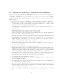
5. (This item also is of interest mainly for the ERGM and ML cases).
The Initial value of gain parameter determines the step sizes in the parameter updates in the
iterative algorithm. A too low value implies that it takes very long to attain a reasonable
parameter estimate when starting from an initial parameter value that is far from the ‘true’
parameter estimate. A too high value implies that the algorithm will be unstable, and may
be thrown off course into a region of unreasonable (e.g., hopelessly large) parameter values.
In the longitudinal case using the Method of Moments (the default estimation procedure),
it usually is unnecessary to change this. In the ERGM case, when the autocorrelations are
smaller than 0.1 but the t statistics for deviations from targets are relatively small
(less than, say, 0.3) but do not all become less than 0.1 in absolute value in repeated runs of
the estimation algorithm, then it will be good to decrease the Initial value of gain parameter.
Do this by dividing it by, e.g., a factor 2 or a factor 5, and then try again a few estimation
runs.
6. If all this is of no avail, then the conclusion may be that the model specification is incorrect
for the given data set.
7. Further help in interpreting output is in Section 7.2 of this manual.
9
3.3
Giving references
When using SIENA, it is appreciated that you refer to this manual and to one or more relevant
references of the methods implemented in the program. The reference to this manual is the
following.
Snijders, Tom A.B., Christian E.G. Steglich, Michael Schweinberger, and Mark Huisman. 2007.
Manual for SIENA version 3. Groningen: University of Groningen, ICS. Oxford: University of
Oxford, Department of Statistics. http://stat.gamma.rug.nl/stocnet
A basic reference for the network dynamics model is Snijders (2001) or Snijders (2005). Basic
references for the model of network-behavior co-evolution are Snijders, Steglich, and Schweinberger
(2007) and Steglich, Snijders, and Pearson (2007).
Basic references for the non-longitudinal (Exponential Random Graph) model are Frank and
Strauss (1986); Wasserman and Pattison (1996); Snijders (2002); and Snijders, Pattison, Robins,
and Handcock (2006). A more didactic reference here is Robins, Snijders, Wang, Handcock, and
Pattison (2007).
More specific references are Schweinberger (2005) for the score-type goodness of fit tests;
Schweinberger and Snijders (2007) for the calculation of standard errors of the Method of Moments
estimators; and Snijders, Koskinen and Schweinberger (2007) for maximum likelihood estimation.
10
Part II
User’s manual
The user’s manual gives the information for using SIENA. It is advisable also to consult the user’s
manual of StOCNET because normally, the user will operate SIENA from within StOCNET.
4
Parts of the program
The operation of the SIENA program is comprised of four main parts:
1. input of basic data description,
2. model specification,
3. estimation of parameter values using stochastic simulation,
4. simulation of the model with given and fixed parameter values.
The normal operation is to start with data input, then specify a model and estimate its parameters, and then continue with new model specifications followed by estimation or simulation.
For the comparison of (nested) models, statistical tests can be carried out.
The program is organized in the form of projects. A project consists of data and the current
model specification. All files internally used in a given project have the same root name, which
is called the project name, and indicated in this manual by pname. (In view of its use for special
simulation purposes, it is advised not to use the project name sisim; also avoid to use the name
siena, which is too general for this purpose.)
The main output is written to the text file pname.out, auxiliary output is contained in the text
files pname.log and pname.eff.
11
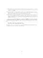
5
Input data
The main statistical method implemented in SIENA is for the analysis of repeated measures of
social networks, and requires network data collected at two or more time points. It is possible
to include changing actor variables (representing behavior, attitudes, outcomes, etc.) which also
develop in a dynamic process, together with the social networks. As repeated measures data on
social networks, at the very least, two or more data files with digraphs are required: the observed
networks, one for each time point. The number of time points is denoted M .
The other statistical method implemented in SIENA if the parameter estimation for the exponential random graph model (‘ERGM ’). For this method, one observed network data set is
required.
In addition, various kinds of variables are allowed:
1. actor-bound or individual variables, also called actor attributes, which can be symbolized as
vi for each actor i; these can be constant over time or changing;
the changing individual variables can be dependent variables (changing dynamically in mutual dependence with the changing network) or independent variables (exogenously changing
variables; then they are also called individual covariates).
2. dyadic covariates, which can be symbolized as wij for each ordered pair of actors (i, j); they
are allowed only to have integer values ranging from 0 to 255. If one has real-valued dyadic
covariates, then one option is to multiply them e.g. by 10 or 100 so that they still have a
range between 0 and 255, and used the rounded values. These likewise can be constant over
time or changing.
All variables must be available in ASCII (‘raw text’) data files, described in detail below.
These files, the names of the corresponding variables, and the coding of missing data, must be
made available to SIENA. In the StOCNET environment, files and variable names are entered in
the Data dialog window, while missing data are identified in the Transformation dialog window. In
the Model dialog window, network data and additional variables subsequently can be selected for
SIENA analyses. This is done by first choosing SIENA from the list of available statistical methods,
and then pushing the Data specification button.
Names of variables must be composed of at most 11 characters. This is because they are used
as parts of the names of effects which can be included in the model, and the effect names should
not be too long. The use of the default variable and file names proposed by StOCNET is not
recommended.
5.1
Digraph data files
Each digraph must be contained in a separate input file. Two data formats are allowed.
1. Adjacency matrices.
The first is an adjacency matrix, i.e., n lines each with n integer numbers, separated by
blanks or tabs, each line ended by a hard return. The diagonal values are meaningless but
must be present.
Although this section talks only about digraphs (directed graphs), it is also possible that all
observed adjacency matrices are symmetric. This will be automatically detected by SIENA,
and the program will then utilize methods for non-directed networks.
The data matrices for the digraphs must be coded in the sense that their values are converted
by the program to the 0 and 1 entries in the adjacency matrix. A set of code numbers is
required for each digraph data matrix; these codes are regarded as the numbers representing
12
a present arc in the digraph, i.e., a 1 entry in the adjacency matrix; all other numbers will
be regarded as 0 entries in the adjacency matrix. Of course, there must be at least one such
code number. All code numbers must be in the range from 0 to 9, except for structurally
determined values (see below).
This implies that if the data are already in 0-1 format, the single code number 1 must be
given. As another example, if the data matrix contains values 1 to 5 and only the values 4
and 5 are to be interpreted as present arcs, then the code numbers 4 and 5 must be given.
2. Pajek format.
If the digraph data file has extension name .net, then the program assumes that the data file
has Pajek format. This can not yet be done when using StOCNET, and therefore this option
is available only when running SIENA outside of StOCNET, as described in Section 16.
The keywords Arcs*, Edges*, Arcslist*, and Edgeslist* are allowed, followed by data
lines according to the Pajek rules. All of these keywords may be used in one input file.
The Edges* and Edgeslist* keywords announce that mutual ties are following. Codes ‘for
present arcs’ as in the adjacency matrix format must be given in the .IN file, but this is only
for consistency in the format for the .IN file, and these codes have no effect. Note that the
Arcslist* and Edgeslist* formats produce binary data anyway. Tie values different from
1, which are used to indicate missings but can also be used for valued data, can only be input
in the Pajek format by using the keywords Arcs* and Edges*.
Code numbers for missing numbers also must be indicated – in the case of either input data
format. These codes must, of course, be different from the code numbers representing present arcs.
Although this section talks only about digraphs (directed graphs), it is also possible that all
observed ties (for all time points) are mutual. This will be automatically detected by SIENA, and
the program will then utilize methods for non-directed networks.
5.1.1
Structurally determined values
It is allowed that some of the values in the digraph are structurally determined, i.e., deterministic
rather than random. This is analogous to the phenomenon of ‘structural zeros’ in contingency
tables, but in SIENA not only structural zeros but also structural ones are allowed. A structural
zero means that it is certain that there is no tie from actor i to actor j; a structural one means
that it is certain that there is a tie. This can be, e.g., because the tie is impossible or formally
imposed, respectively.
Structural zeros provide an easy way to deal with actors leaving or joining the network between
the start and the end of the observations. Another way (more complicated but it gives possibilities
to represent actors entering or leaving at specified moments between observations) is described in
Section 5.7.
Structurally determined values are defined by reserved codes in the input data: the value 10
indicates a structural zero, the value 11 indicates a structural one. Structurally determined values
can be different for the different time points. (The diagonal of the data matrix always is composed
of structural zeros, but this does not have to be indicated in the data matrix by special codes.)
The correct definition of the structurally determined values can be checked from the brief report
of this in the output file, and by looking at the file pname.s01 (for the first time point), pname.s02
(second time point), etc. In these files, the structurally determined positions (structural zeros as
well as structural ones) are indicated by the value 1, all others (i.e., the positions where ties are
random) by the value 0.
Structural zeros offer the possibility of analyzing several networks simultaneously under the
assumption that the parameters are identical. E.g., if there are three networks with 12, 20 and 15
13
actors, respectively, then these can be integrated into one network of 12 + 20 + 15 = 47 actors, by
specifying that ties between actors in different networks are structurally impossible. This means
that the three adjacency matrices are combined in one 47×47 data file, with values 10 for all entries
that refer to the tie from an actor in one network to an actor in a different network. In other words,
the adjacency matrices will be composed of three diagonal blocks, and the off-diagonal blocks will
have all entries equal to 10. In this example, the number of actors per network (12 to 20) is rather
small to obtain good parameter estimates, but if the additional assumption of identical parameter
values for the three networks is reasonable, then the combined analysis may give good estimates.
In such a case where K networks (in the preceding paragraph, the example had K = 3) are
combined artificially into one bigger network, it will often be helpful to define K − 1 dummy
variables at the actor level to distinguish between the K components. These dummy variables can
be given effects in the rate function and in the evaluation function (for “ego”), which then will
represent that the rate of change and the out-degree effect are different between the components,
while all other parameters are the same.
5.2
Dyadic covariates
As the digraph data, also each measurement of a dyadic covariate must be contained in a separate
input file with a square data matrix, i.e., n lines each with n integer numbers, separated by blanks
or tabs, each line ended by a hard return. The diagonal values are meaningless but must be present.
Pajek input format is currently not possible for dyadic covariates.
A distinction is made between constant and changing dyadic covariates, where change refers to
changes over time. Each constant covariate has one value for each pair of actors, which is valid
for all observation moments, and has the role of an independent variable. Changing covariates, on
the other hand, have one such value for each period between measurement points. If there are M
waves of network data, this covers M − 1 periods, and accordingly, for specifying a single changing
dyadic covariate, M − 1 data files with covariate matrices are needed.
The StOCNET interface requires the user to enter these in blocks of M − 1, and within each
block in sequential order. This is done in the Data specification menu of the SIENA model page. For
each such block, also a name must be provided to identify the changing dyadic covariate. For data
sets with only two waves, the specification of changing dyadic covariates is meaningless, because
there is only one period, hence there is no change over periods possible. Constant dyadic covariates
can be selected in the respective section of the Data specification menu. They are identified by the
name given to them in the initial Data step in StOCNET.
The reasons for restricting dyadic covariates to integer values from 0 to 255 are historical and
have to do with how the constant dyadic covariate data are stored internally. If the user wishes
to use a dyadic covariate with a different range, this variable first must be transformed to integer
values from 0 to 255. E.g., for a continuous variable ranging from 0 to 1, the most convenient way
probably is to multiply by 100 (so the range becomes 0–100) and round to integer values. In the
current implementation, this type of recoding cannot easily be carried out within StOCNET, but
the user must do it in some other program.
The mean is always subtracted from the covariates. See the section on Centering.
5.3
Individual covariates
Individual (i.e., actor-bound) variables can be combined in one or more files. If there are k variables
in one file, then this data file must contain n lines, with on each line k numbers which all are read
as real numbers (i.e., a decimal point is allowed). The numbers in the file must be separated by
blanks and each line must be ended by a hard return. There must not be blank lines after the last
data line.
14
Also here, a distinction is made between constant and changing actor variables. Each constant
actor covariate has one value per actor valid for all observation moments, and has the role of an
independent variable.
Changing variables can change between observation moments. They can have the role of dependent variables (changing dynamically in mutual dependence with the changing network) or
of independent variables; in the latter case, they are also called ‘changing individual covariates’.
Dependent variables are treated in the section below, this section is about individual variables in
the role of independent variables – then they are also called individual covariates.
When changing individual variables have the role of independent variables, they are assumed
to have constant values from one observation moment to the next. If observation moments for
the network are t1 , t2 , ..., tM , then the changing covariates should refer to the M − 1 moments
t1 through tM −1 , and the m-th value of the changing covariates is assumed to be valid for the
period from moment tm to moment tm+1 . The value at tM , the last moment, does not play a
role. Changing covariates, as independent variables, are meaningful only if there are 3 or more
observation moments, because for 2 observation moments the distinction between constant and
changing covariates is not meaningful.
Each changing individual covariate must be given in one file, containing k = M − 1 columns
that correspond to the M − 1 periods between observations. It is not a problem if there is an M ’th
column in the file, but it will not be read.
The mean is always subtracted from the covariates. See the section on Centering.
5.4
Interactions and dyadic transformations of covariates
For actor covariates, two kinds of transformations to dyadic covariates are made internally in
SIENA. Denote the actor covariate by vi , and the two actors in the dyad by i and j. Suppose that
the range of vi (i.e., the difference between the highest and the lowest values) is given by rV . The
two transformations are the following:
1. dyadic similarity, defined by 1− |vi −vj |/rV , and centered so the the mean of this similarity
variable becomes 0;
note that before centering, the similarity variable is 1 if the two actors have the same value,
and 0 if one has the highest and the other the lowest possible value;
2. dyadic identity, defined by 1 if vi = vj , and 0 otherwise (not centered).
In addition, SIENA offers the possibility of user-defined two- and three-variable interactions
between covariates; see Section 6.6.
5.5
Dependent action variables
SIENA also allows dependent action variables, also called dependent behavior variables. This can be
used in studies of the co-evolution of networks and behavior, as described in Snijders, Steglich, and
Schweinberger (2007) and Steglich, Snijders, and Pearson (2007). These action variables represent
the actors’ behavior, attitudes, beliefs, etc. The difference between dependent action variables and
changing actor covariates is that the latter change exogenously, i.e., according to mechanisms not
included in the model, while the dependent action variables change endogenously, i.e., depending on
their own values and on the changing network. In the current implementation only one dependent
network variable is allowed, but the number of dependent action variable can be larger than one.
Unlike the changing individual covariates, the values of dependent action variables are not assumed
to be constant between observations.
15
Dependent action variables must have nonnegative integer values; e.g., 0 and 1, or a range of
integers like 0,1,2 or 1,2,3,4,5. Each dependent action variable must be given in one file, containing
k = M columns, corresponding to the M observation moments.
5.6
Missing data
SIENA allows that there are some missing data on network variables, on covariates, and on dependent action variables. Missing data in changing dyadic covariates are not yet implemented.
Missing data must be indicated by missing data codes (this can be specified in StOCNET, if SIENA
is operated through StOCNET ), not by blanks in the data set.
In the current implementation of SIENA, missing data are treated in a simple way, trying to
minimize their influence on the estimation results. The simulations are carried out over all actors.
Missing data are treated separately for each period between two consecutive observations of the
network. In the initial observation for each period, missing entries in the adjacency matrix are set
to 0, i.e., it is assumed that there is no tie. Missing covariate data as well as missing entries on
dependent action variables are replaced by the variable’s average score at this observation moment.
In the course of the simulations, however, the adjusted values of the dependent action variables
and of the network variables are allowed to change.
In order to ensure a minimal impact of missing data treatment on the results of parameter
estimation (method of moments estimation) and/or simulation runs, the calculation of the target
statistics used for these procedures is restricted to non-missing data. When for an actor in a given
period, any variable is missing that is required for calculating a contribution to such a statistic, this
actor in this period does not contribute to the statistic in question. For network and dependent
action variables, an actor must provide valid data both at the beginning and at the end of a period
for being counted in the respective target statistics.
5.7
Composition change
SIENA can also be used to analyze networks of which the composition changes over time, because
actors join or leave the network between the observations. This can be done in two ways: using the
method of Huisman and Snijders (2003), or using structural zeros. (For the maximum likelihood
estimation option, the Huisman-Snijders method is not implemented, and only the structural zeros
method can be used.) Structural zeros can specified for all elements of the tie variables toward
and from actors who are absent at a given observation moment. How to do this is described in
subsection 5.1.1. This is straightforward and not further explained here.2 This subsection explains
the method of Huisman and Snijders (2003).
For this case, a data file is needed in which the times of composition change are given. For
networks with constant composition (no entering or leaving actors), this file is omitted and the
current subsection can be disregarded.
Network composition change, due to actors joining or leaving the network, is handled separately
from the treatment of missing data. The digraph data files must contain all actors who are part of
the network at any observation time (denoted by n) and each actor must be given a separate (and
fixed) line in these files, even for observation times where the actor is not a part of the network
(e.g., when the actor did not yet join or the actor already left the network). In other words, the
adjacency matrix for each observation time has dimensions n × n.
At these times, where the actor is not in the network, the entries of the adjacency matrix can
be specified in two ways. First as missing values using missing value code(s). In the estimation
procedure, these missing values of the joiners before they joined the network are regarded as 0
2 In the Siena01 program there is an option, which can be activated upon request by the programmers, to
automatically convert
16
entries, and the missing entries of the leavers after they left the network are fixed at the last
observed values. This is different from the regular missing data treatment. Note that in the
initial data description the missing values of the joiners and leavers are treated as regular missing
observations. This will increase the fractions of missing data and influence the initial values of the
density parameter.
A second way is by giving the entries a regular observed code, representing the absence or
presence of an arc in the digraph (as if the actor was a part of the network). In this case, additional
information on relations between joiners and other actors in the network before joining, or leavers
and other actors after leaving can be used if available. Note that this second option of specifying
entries always supersedes the first specification: if a valid code number is specified this will always
be used.
For joiners and leavers, crucial information is contained in the times they join or leave the
network (i.e., the times of composition change), which must be presented in a separate input file.
This data file must contain n lines, each line representing the corresponding actor in the digraph
files, with on each line four numbers. The first two concern joiners, the last two concern leavers:
1) the last observation moment at which the actor is not yet observed, 2) the time of joining
(expressed as a fraction of the length of the period), 3) the last observation moment at which the
actor is observed, 4) the time of leaving (also expressed as a fraction). Also actors who are part of
the network at all observation moments must be given values in this file. In the following example,
the number of observation moments is considered to be M = 5, which means there are four periods;
period m starts at observation moment m and ends at m + 1 for m = 1, 2, ..., 4 = M − 1.
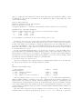
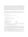
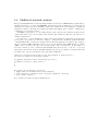
Example of file with times of composition change
Present at all five observation times
Joining in period 2 at fraction 0.6 of length of period
Leaving in period 3 at fraction 0.4 of length of period
Joining in per. 1 (0.7) and leaving in per. 4 (0.2)
Leaving in per. 2 (0.6) and joining in per. 3 (0.8)
0
2
0
1
3
1.0
0.6
1.0
0.7
0.8
5
5
3
4
2
0.0
0.0
0.4
0.2
0.6
Note that for joining, the numbers 0 1.0 have a different meaning than the numbers 1 0.0.
The former numbers indicate that an actor is observed at time 1 (he/she joined the network right
before the first time point), the latter indicate that an actor is not observed at observation time
1 (he/she joined just after the first time point). The same holds for leavers: 5 0.0 indicates that
an actor is observed at time point 5, whereas 4 1.0 indicates that an actor left right before he/she
was observed at time point 5.
From the example it follows that an actor is only allowed to join, leave, join and then leave,
or leave and then join the network. The time that the actor is part of the network must be an
uninterrupted period. It is not allowed that an actor joins twice or leaves twice. When there is no
extra information about the time at which an actor joins or leaves (in some known period), there
are three options: set the fraction equal to 0.0, 0.5, or 1.0. The second option is thought to be
least restrictive.
The following special options are available for treatment of composition change by indicating
this in the corresponding line in the .IN file (see Section 19.1):
2. The values of the joiners before joining are replaced by the value 0 (no ties), and the values
of the leavers after leaving are treated as regular missing data.
3. The values of the joiners before joining and the values of the leavers after leaving are treated
as regular missing data.
17
4. Before joining and after leaving, actors are treated as structural zeros.
Option 4 has the same effect as specifying the data for the absent actors as structural zeros; this
option is useful for users who have a data set ready with joiners and leavers and wish to transform
it automatically to a data set with structural zeros, e.g., because they wish to use the maximum
likelihood estimation procedure.
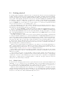
5.8
Centering
Individual as well as dyadic covariates are centered by the program in the following way.
For individual covariates, the mean value is subtracted immediately after reading the variables.
For the changing covariates, this is the global mean (averaged over all periods). The values of
these subtracted means are reported in the output.
For the dyadic covariates and the similarity variables derived from the individual covariates, the
grand mean is calculated, stored, and subtracted during the program calculations. (Thus, dyadic
covariates are treated by the program differently than individual covariates in the sense that the
mean is subtracted at a different moment, but the effect is exactly the same.)
The formula for balance is a kind of dissimilarity between rows of the adjacency matrix. The
mean dissimilarity is subtracted in this formula and also reported in the output. This mean
dissimilarity is calculated by a formula given in Section 15.
The dependent network variable and the dependent action variables are not centered.
18
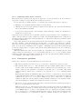
6
Model specification
After defining the data, the next step is to specify a model. In the StOCNET environment, this is
done by clicking the Model specification button that is activated after a successful Data specification
in StOCNET ’s Model menu, provided that SIENA was selected from the list of available models.
The model specification consists of a selection of ‘effects’ for the evolution of each dependent
variable (network or behavior). A list of all available effects for a given SIENA project is given in
the secondary output file pname.log. A list of all effects in the objective function is given in the
file pname.eff.
For the longitudinal case, three types of effects are distinguished (see Snijders, 2001; Steglich,
Snijders and Pearson, 2007):
• rate function effects
The rate function models the speed by which the dependent variable changes; more precisely:
the speed by which each network actor gets an opportunity for changing her score on the
dependent variable.
Advice: in most cases, start modeling with a constant rate function without additional rate
function effects. Constant rate functions are selected by exclusively checking the ‘basic rate
parameter’ (for network evolution) and the main rate effects (for behavioral evolution) on
the model specification screen. (When there are important size or activity differences between
actors, it is possible that different advice must be given, and it may be necessary to let the
rate function depend on the individual covariate that indicates this size; or on the out-degree.)
• evaluation function effects
The evaluation function3 models the network actors’ satisfaction with their local network
neighborhood configuration. It is assumed that actors change their scores on the dependent
variable such that they improve their total satisfaction – with a random element to represent
the limited predictability of behavior. In contrast to the endowment function (described
below), the evaluation function evaluates only the local network neighborhood configuration
that results from the change under consideration. In most applications, the evaluation function will be the main focus of model selection.
The network evaluation function normally should always contain the ‘density’, or ‘out-degree’
effect, to account for the observed density. For directed networks, it mostly is also advisable
to include the reciprocity effect, this being one of the most fundamental network effects. Likewise, behavior evaluation functions should normally always contain the tendency parameter,
to account for the observed prevalence of the behavior.
• endowment function effects
The endowment function4 is an extension of the evaluation function that allows to distinguish
between new and old network ties (when evaluating possible network changes) and between
increasing or decreasing behavioral scores (when evaluating possible behavioral changes).
The function models the loss of satisfaction incurred when existing network ties are dissolved
or when behavioral scores are decreased to a lower value (hence the label ‘endowment’).
Advice: start modeling without any endowment effects, and add them at a later stage.
The estimation and simulation procedures of SIENA operate on the basis of the model specification which comprises the set of effects included in the model as described above, together
with the current parameter values and the Model Type (see Section 6.5). After data input, the
3 The
4 The
evaluation function was called objective function in Snijders, 2001.
endowment function is similar to the gratification function in Snijders, 2001.
19
constant rate parameters and the density effect in the network evaluation function have default
initial values, depending on the data. All other parameter values initially are 0. The estimation
process changes the current value of the parameters to the estimated values. Values of effects not
included in the model are not changed by the estimation process. It is possible for the user to
change parameter values and to request that some of the parameters are fixed in the estimation
process at their current value.
6.1
Important structural effects for network dynamics
For the structural part of the model for network dynamics, the most important effects are as
follows. The mathematical formulae for these and other effects are given in Section 15. Here we
give a more qualitative description.
1. The out-degree effect which always must be included.
2. The reciprocity effect which practically always must be included.
3. There is a choice of four network closure effects. Usually it will be sufficient to express
the tendency to network closure by including one or two of these. They can be selected by
theoretical considerations and/or by their empirical statistical significance. Some researchers
may find the last effect (distances two) less appealing because it expresses network closure
inversely.
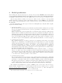
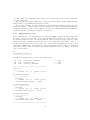
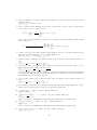
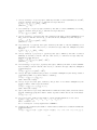
a. The transitive triplets effect, which is the classical representation of network closure by the number of transitive
triplets. For this effect the contribution of the tie i → j
is proportional to the total number of transitive triplets
that it forms – which can be transitive triplets of the type
{i → j → h; i → h} as well as {i → h → j; i → j};
h
•
. ...
........... ...........
...
..
...
...
.
.
...
...
...
..
...
.
.
...
...
.
...
..
.
...
..
....................................................
•
•
i
j
b. The balance effect, which may also be called structural equivalence with respect to outgoing ties. This expresses a preference of actors to have ties to those other actors who
have a similar set of outgoing ties as themselves. Whereas the transitive triplets effect
focuses on how many same choices are made by ego (the focal actor) and alter (the
other actor) — the number of h for which i → h and j → h, i.e., xih = xjh = 1 where
i is ego and j is alter — , the balance effect considers in addition how many the same
non-choices are made — xih = xjh = 0.
c. The direct and indirect ties effect is similar to the transitive triplets effect, but instead
of considering for each other actor j how many two-paths i → h → j there are, it is only
considered whether there is at least one such indirect connection. Thus, one indirect tie
suffices for the network embeddedness.
d. The distances two effect expresses network closure inversely: stronger network closure
(when the total number of ties is fixed) will lead to less geodesic distances equal to 2.
When this effect has a negative parameter, actors will have a preference for having few
others at a geodesic distance of 2 (given their out-degree, which is the number of others
at distance 1); this is one of the ways for expressing network closure.
20
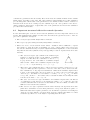
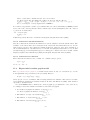
4. The three-cycles effect, which can be regarded as generalized reciprocity (in an exchange interpretation of the network) but also as
the opposite of hierarchy (in a partial order interpretation of the network). A negative three-cycles effect sometimes may be interpreted as
a tendency toward hierarchy. The three-cycles effect also contributes
to network closure.
In a non-directed network, the three-cycles effect is identical to the
transitive triplets effect.
h
•
.. ...
... ........
.. ......
..
...
...
...
...
...
...
...
.
.
.
...
.
.
...
...........
...
...
.
....................................................
•
•
i
j
5. Another triadic effect is the betweenness effect, which represents brokerage: the tendency for
actors to position themselves between not directly connected others, i.e., a preference of i for
ties i → j to those j for which there are many h with h 6→ j.
6. The distribution of degrees can be modeled more closely by using the effects sum of (1/(outdegree + 1) and/or the other effects defined by non-linear functions of out-degrees.
6.2
Effects for network dynamics associated with covariates
For each individual covariate, there are several effects which can be included in a model specification, both in the network evolution part and in the behavioral evolution part (should there be
dependent behavior variables in the data).
• network rate function
1. the covariate’s effect on the rate of network change of the actor;
• network evaluation and endowment functions
1. the covariate-similarity effect; a positive parameter implies that actors prefer ties to others with similar values on this variable – thus contributing to the network-autocorrelation
of this variable not by changing the variable but by changing the network;
2. the effect on the actor’s activity (covariate-ego); a positive parameter will imply the
tendency that actors with higher values on this covariate increase their out-degrees
more rapidly;
3. the effect on the actor’s popularity to other actors (covariate-alter); a positive parameter
will imply the tendency that the in-degrees of actors with higher values on this covariate
increase more rapidly;
4. the interaction between the value of the covariate of ego and of the other actor (covariate
ego × covariate alter); a positive effect here means, just like a positive similarity effect,
that actors with a higher value on the covariate will prefer ties to others who likewise
have a relatively high value; this effect is quite analogous to the similarity effect, and
for dichotomous covariates, in models where the ego and alter effects are also included,
it even is equivalent to the similarity effect (although expressed differently);
5. the covariate identity effect, which expresses the tendency of the actors to be tied to
others with exactly the same value on the covariate; whereas the preceding four effects
are appropriate for interval scaled covariates (and mostly also for ordinal variables), the
identity effect is suitable for categorical variables;
6. the interaction effect of covariate-similarity with reciprocity.
21
The usual order of importance of these covariate effects on network evolution is: evaluation effects
are most important, followed by endowment and rate effects. Inside the group of evaluation effects,
it is the covariate-similarity effect that is most important, follwed by the effects of covariate-ego
and covariate-alter.
For each dyadic covariate, the following network evaluation effects can be included in the model
for network evolution:
• network evaluation and endowment functions
1. main effect of the dyadic covariate;
2. the interaction effect of the dyadic covariate with reciprocity.
The main evaluation effect is usually the most important. In the current version of SIENA, there
are no effects of dyadic covariates on behavioral evolution.
6.3
Effects on behavior evolution
For models with a dependent behavior variable in models for the co-evolution of networks and
behavior, the most important effects for the behavior dynamics are the following. In these descriptions, with the ‘alters’ of an actor we refer to the other actors to whom the focal actor has an
outgoing tie.
1. The tendency effect, expressing the basic drive toward high values. A zero value for the
tendency will imply a drift toward the midpoint of the range of the behavior variable.
2. The effect of the behavior on itself, which is relevant only if the number of behavioral categories is 3 or more. This can be interpreted as giving a quadratic preference function for the
behavior. With a negative coefficient, this represents that the most desired behavior can lie
somewhere between the minimum and maximum values of the behavioral variable.
3. The average similarity effect, expressing the preference of actors to being similar to their
alters, where the total influence of the alters is the same regardless of the number of alters.
4. The total similarity effect, expressing the preference of actors to being similar to their alters,
where the total influence of the alters is proportional to the number of alters.
5. The average alter effect, expressing that actors whose alters have a higher average value of
the behavior, also have themselves a stronger tendency toward high values on the behavior.
6. The indegree effect, expressing that actors with a higher indegree (more ‘popular’ actors)
have a stronger tendency toward high values on the behavior.
7. The outdegree effect, expressing that actors with a higher outdegree (more ‘active’ actors)
have a stronger tendency toward high values on the behavior.
Effects 1 and 2 will practically always have to be included as control variables. (For dependent
behavior variables with 2 categories, this applies only to effect 1.)
The average similarity, total similarity, and average alter effects are different specifications of
social influence. The choice between them will be made on theoretical grounds and/or on the basis
of statistical significance.
22
6.4
Exponential Random Graph Models
For the non-longitudinal (‘ERGM’) case, default advice is given in Snijders et al. (2006) and in
Robins et al. (2007). The basic structural part of the model is comprised, for directed networks,
by the following effects.
1. The reciprocity effect.
2. The alternating k-out-stars effect to represent the distribution of the out-degrees.
3. The alternating k-in-stars effect to represent the distribution of the in-degrees.
4. For alternating transitive k-triangles effect to represent the tendency to transitivity.
5. The alternating independent two-paths effect to represent the preconditions for transitivity,
or alternatively, the association between in-degrees and out-degrees.
6. The number of three-cycles to represent cyclicity, or generalized reciprocity, or the converse
of hierarchy.
For nondirected networks. the basic structural part is comprised by the following, smaller, set.
1. The alternating k-stars effect to represent the distribution of the degrees.
2. For alternating transitive k-triangles effect to represent the tendency to transitivity.
3. The alternating independent two-paths effect to represent the preconditions for transitivity,
or alternatively, the association between in-degrees and out-degrees.
Other effects can be added to improve the fit.
To obtain good convergence results for the ERGM case, it will usually be necessary to increase
the default value of the multiplication factor; see Sections 3.2 and 11.
6.5
Model Type
When the data is perfectly symmetric, this will be detected by SIENA. Then the analysis options
for nondirected networks will be followed.
6.5.1
Model Type: directed networks
For directed networks, the Model Type distinguishes between the model of Snijders (2001) (Model
Type 1), that of Snijders (2003) (Model Type 2), and the tie-based model described in Snijders
(2006) (Model Type 3). Model Type 1 is the default model and is described in the basic publications
on Stochastic Actor-Oriented Models for network dynamics.
Model type 2 is at this moment not implemented in SIENA version 3.
In Model Type 2, the ‘decisions’ by the actors consist of two steps: first a step to increase or
decrease their out-degree; when this step has been taken, the selection of the other actor towards
whom a new tie is extended (if the out-degree rises) or from a an existing tie is withdrawn (if the
out-degree drops). The decision by an actor to increase or decrease the number of outgoing ties
is determined on the basis of only the current degree; the probabilities of increasing or decreasing
the out-degree are expressed by the distributional tendency function ξ (indicated in the output as
xi ) and the volatility function ν (indicated as nu). Which new tie to create, or which existing tie
to withdraw, depends in the usual way on the evaluation and endowment functions. Thus, the
outdegree distribution is governed by parameters that are not connected to the parameters for the
23
structural dynamics. The use of such an approach in statistical modeling minimizes the influence
of the observed degrees on the conclusions about the structural aspects of the network dynamics.
This is further explained in Snijders (2003).
For Model Type 2, in the rate function, effects connected to these functions ξ and ν are
included. On the other hand, effects in the evaluation function that depend only on the outdegrees are canceled from the model specification, because they are not meaningful in Model
Type 2. To evaluate whether Model Type 1 or Model Type 2 gives a better fit to the observed
degree distribution, the output gives a comparison between the observed out-degrees and the fitted
distribution of the out-degrees (as exhibited by the simulated out-degrees). For Model Type 2 this
comparison is always given. For Model Type 1, this comparison is given by adding 10 to the Model
Code in the advanced options. (For LATEX users: the log file contains code that can be used to
make a graph of the type given in Snijders, 2003).
For using Model Type 2, it is advised to first estimate some model according to Model Type
1 (this may be a simple model containing a reciprocity effect only, but it could also include more
effects), and then – using the parameters estimated under Model Type 1 – change the specification
to Model Type 2, and use the unconditional estimation method (see Section 7.3.4) (instead of the
conditional method which is the default). It is likely that the very first model estimated under
Model Type 2 will have results with poor convergence properties, but in such cases it is advised
just to estimate the same model another time, now using the parameter values obtained under the
previous Model Type 2 run as the initial values for the estimation.
To obtain a good model specification with respect to the rates of change in dependence of the
out-degrees, three effects can be included:
1. the out-degrees effect
2. the factorial out-degree effect
3. the logarithmic out-degree effect.
These are the effects defined in formula (18) of Snijders (2003b) and indicated with the parameters
α1 , α2 , and α3 , respectively. The user has to see from the estimation results which, or which two,
out of these effects should be included to yield a good fit for the out-degrees.
In addition these types, there is Model Type 6 which implements the reciprocity model of
Wasserman (1979) and Leenders (1995) (also see Snijders, 1999, 2005) — provided that no other
effects are chosen than the outdegree effect, the reciprocity effect and perhaps the reciprocity
endowment effect, and possible also effects of actor covariates or dyadic covariates. This model
is meaningful only as a “straw man” model to provide a test of the null hypothesis that the
dynamics of the dyads are mutually independent, against the alternative hypothesis that there
do exist network effects (which make the dyad processes mutually dependent). For this purpose,
Model Type 6 can be chosen, while for one or more network effects such as the effects representing
transitivity, the null hypothesis is tested that their coefficients are zero (see Section 9).
The Model Type is specified in the model options as (part of) the Model Code.
6.5.2
Model Type: non-directed networks
Non-directed networks are an undocumented option (there currently only is the presentation Snijders 2007), and therefore mentioned here reluctantly for those users who want to use this option
anyway.
SIENA detects automatically when the networks all are non-directed, and then employs a model
for this special case. For non-directed networks, the Model Type has seven possible values, as
described in Snijders (2007).
24
1. Forcing model:
one actor takes the initiative and unilaterally imposes that a tie is created or dissolved.
2. Unilateral initiative and reciprocal confirmation:
one actor takes the initiative and proposes a new tie or dissolves an existing tie; if the actor
proposes a new tie, the other has to confirm, otherwise the tie is not created.
3. Tie-based model:
a random pair of actors is chosen (actor-specific rate functions are not used here), and the
average change in objective function (1) for toggling (i, j) and (j, i) is the log-odds of the
probability of changing the tie variable.
4. Pairwise conjunctive model:
a pair of actors is chosen and reconsider whether a tie will exist between them; a new tie is
formed if both agree.
5. Pairwise disjunctive (forcing) model:
a pair of actors is chosen and reconsider whether a tie will exist between them; a new tie is
formed if at least one wishes this.
6. Pairwise compensatory (additive) model:
a pair of actors is chosen and reconsider whether a tie will exist between them; this is based
on the sum of their utilities for the existence of this tie.
In Models 1-2, where the initiative is one-sided, the rate function is comparable to the rate function
in directed models. In Models 4-6, however, the pair of actors is chosen at a rate which is the product
of the rate functions λi and λj for the two actors. This means that opportunities for change of
the single tie variable xij occur at the rate λi × λj . The numerical interpretation is different from
that in Models 1-2.
6.6
Additional interaction effects
It is possible for the user to define additional interaction effects for the network. This applies
both to longitudinal and non-longitudinal (ERG) modeling. The basis is provided by the initial
definition, by SIENA, of “unspecified interaction effects”. Modifying the internal effect parameters
of these effects allows the definition of two-way or three-way interactions. Not all user-defined
interactions are possible:
• For longitudinal models:
Ego effects of actor variables can interact with all effects. Further, interaction effects are
permitted which are combinations of actor variables, dyadic variables, and reciprocity.
• For non-longitudinal (ERG) models:
Actor covariates and dyadic covariates can interact with each other and with reciprocity.
The specification is made by changing the internal effect parameter for the interaction effects.
The values of these internal parameters can be changed in the pname.mo file described in Section 19.2.1. In StOCNET, they are accessible as the “par.” column in the Advanced Options
screen of the Model Specification.
For interaction effects, this parameter represents a code for the two or three interacting effects.
Each effect is represented by its index number in three digits (including leading zeros) as reported
in the file called pname.eff (recall that pname stands for your project name). Thus, two-way
interactions are represented by twice three digits: e.g., the code 020003 refers to the interaction
25
between the effects numbered 20 and 3, where the numbers are the rank numbers in this list of
all effects. Leading zeros of the total parameter can be skipped, so that the code 020003 can also
be represented by 20003 (but not by 203!). The order does not matter, so that the codes 020003,
003020, 20003, and 3020 all are equivalent. Three-way interactions similarly are represented by
thrice three digits. For example, the code 020028003 represents the interaction effects between
the effects numbered 20, 28, and 3. E.g., to implement the interaction effect between the effects
numbered 20 and 3, in the pname.mo file the lines that initially are
unspecified interaction effect
0 0 0 0
0.000000 0
0 0 0 0
0.000000 0
0 0 0 0
0.000000 0
must be changed into
unspecified interaction effect
0 0 0 0
0.000000 020003
0 0 0 0
0.000000 0
0 0 0 0
0.000000 0
After this is done, SIENA will automatically replace the name by the suitable interaction effect
name.
The calculation of user-defined effects is slightly more time-consuming than the calculation of
internally defined effects. Therefore, when there is the choice between two equivalent effects – e.g.,
in longitudinal modeling, interactions of actor covariates with reciprocity – then it is advisable to
use the predefined interaction effects.
26
7
Estimation
The model parameters are estimated under the specification given during the model specification
part, using a stochastic approximation algorithm. Three estimation procedures are implemented:
the Method of Moments (MoM) (Snijders, 2001; Snijders, Steglich, and Schweinberger, 2007);
the Method of Maximum Likelihood (ML) (Snijders, Koskinen and Schweinberger, 2007); and
a Bayesian method (Koskinen, 2005; Koskinen and Snijders, 2007; Schweinberger and Snijders,
2007). For non-constant rate functions, currently only MoM estimation is available. The Method
of Moments is the default; the other two methods require much more computing time. Given the
greater efficiency but longer required computing time for the ML and Bayesian methods, these
can be useful especially for smaller data sets and relatively complicated models (networks and
behavior; endowment effects).
In the following, the number of parameters is denoted by p. The algorithms are based on
repeated (and repeated, and repeated...) simulation of the evolution process of the network. These
repetitions are called ‘runs’ in the following. The MoM estimation algorithm is based on comparing
the observed network (obtained from the data files) to the hypothetical networks generated in the
simulations.
Note that the estimation algorithm is of a stochastic nature, so the results can vary! This is of
course not what you would like. For well-fitting combinations of data set and model, the estimation
results obtained in different trials will be very similar. It is good to repeat the estimation process
at least once for the models that are to be reported in papers or presentations, to confirm that
what you report is a stable result of the algorithm.
The initial value of the parameters normally is the current value (that is, the value that the
parameters have immediately before you start the estimation process); as an alternative, it is
possible to start instead with a standard initial value. Usually, a sequence of models can be fitted
without problems, each using the previously obtained estimate as the starting point for the new
estimation procedure. Sometimes, however, problems may occur during the estimation process,
which will be indicated by some kind of warning in the output file or by parameter estimates
being outside a reasonably expected range. In such cases the current parameter estimates may be
unsatisfactory, and using them as initial values for the new estimation process might again lead to
difficulties in estimation. Therefore, when the current parameter values are unlikely and also when
they were obtained after a divergent estimation algorithm, it is advisable to start the estimation
algorithm with a standard initial value. The use of standard initial values is one of the model
options.
7.1
Algorithm
During the estimation process, StOCNET transfers control to the SIENA program. The estimation
algorithm has for both the MoM and ML method three phases:
1. In phase 1, the parameter vector is held constant at its initial value. This phase is for having
a first rough estimate of the matrix of derivatives.
2. Phase 2 consists of several subphases. More subphases means a greater precision. The
default number of subphases is 4. The parameter values change from run to run, reflecting
the deviations between generated and observed values of the statistics. The changes in the
parameter values are smaller in the later subphases.
The program searches for parameter values where these deviations average out to 0. This
is reflected by what is called the ‘quasi-autocorrelations’ in the output screen. These are
averages of products of successively generated deviations between generated and observed
statistics. It is a good sign for the convergence of the process when the quasi-autocorrelations
27
are negative (or positive but close to 0), because this means the generated values are jumping
around the observed values.
3. In phase 3, the parameter vector is held constant again, now at its final value. This phase is
for estimating the covariance matrix and the matrix of derivatives used for the computation
of standard errors.
The default number of runs in phase 3 is 1000. This requires a lot of computing time,
but when the number of phase 3 runs is too low, the standard errors computed are rather
unreliable.
The number of subphases in phase 2, and the number of runs in phase 3, can be changed in
the model options.
The user can break in and modify the estimation process in three ways:
1. it is possible to terminate the estimation;
2. in phase 2, it is possible to terminate phase 2 and continue with phase 3;
3. in addition, it is possible to change the current parameter values and restart the whole
estimation process.
For the ML estimation option and for the non-longitudinal case, tuning the ‘multiplicaton
factor’ and the ‘initial gain parameter’ can be important for getting good results; for Bayesian
estimation the ‘multiplicaton factor’ can likewise be important; this is briefly described in Section 3.2.
7.2
Output
There are three output files. All are ASCII (‘text’) files which can be read by any text editor. The
main output is given in the pname.out file (recall that pname is the project name defined by the
user). A brief history of what the program does is written to the file pname.log. The latter file also
contains some supplementary output that usually is disregarded but sometimes is helpful. Some
diagnostic output containing a history of the estimation algorithm which may be informative when
there are convergence problems is written to the file pname.cck (for ‘check’). This file is overwritten
for each new estimation. Normally, you only need to look at pname.out.
The output is divided into sections indicated by a line @1, subsections indicated by a line @2,
subsubsections indicated by @3, etc. For getting the main structure of the output, it is convenient
to have a look at the @1 marks first.
The primary information in the output of the estimation process consists of the following three
parts. Results are presented here which correspond to Table 2, column “t1 , t3 ” of Snijders (2001).
The results were obtained in an independent repetition of the estimation for this data set and
this model specification; since the repetition was independent, the results are slightly different,
illustrating the stochastic nature of the estimation algorithm.
1. Convergence check
In the first place, a convergence check is given, based on Phase 3 of the algorithm. This check
considers the deviations between simulated values of the statistics and their observed values (the
latter are called the ‘targets’). Ideally, these deviations should be 0. Because of the stochastic
nature of the algorithm, when the process has properly converged the deviations are small but not
exactly equal to 0. The program calculates the averages and standard deviations of the deviations
and combines these in a t-statistic (in this case, average divided by standard deviation). For
longitudinal modeling, convergence is excellent when these t-values are less than 0.1 in absolute
28
value, good when they are less than 0.2, and moderate when they are less than 0.3. (These bounds
are indications only, and are not meant as severe limitations.) The corresponding part of the
output is the following.
Total of 1954 iterations.
Parameter estimates based on 954 iterations,
basic rate parameter as well as
convergence diagnostics, covariance and derivative matrices based on 1000 iterations.
Information for convergence diagnosis.
Averages, standard deviations, and t-ratios for deviations from targets:
1.
-0.236
7.006
-0.034
2.
0.204
7.059
0.029
3.
-1.592
22.242
-0.072
Good convergence is indicated by the t-ratios being close to zero.
In this case, the t-ratios are -0.034, -0.029, and -0.072, which is less than 0.1 in absolute value,
so the convergence is excellent. In data exploration, if one or more of these t-ratios are larger in
absolute value than 0.3, it is advisable to restart the estimation process. For results that are to be
reported, it is advisable to carry out a new estimation when one or more of the t-ratios are larger
in absolute value than 0.1. Large values of the averages and standard deviations are in themselves
not at all a reason for concern.
For the exponential random graph (or p∗ ) model, the convergence of the algorithm is more
problematic than for longitudinal modeling. A sharper value of the t-ratios must be found before
the user may be convinced of good convergence. It is advisable to try and obtain t-values which are
less than 0.15. If, even with repeated trials, the algorithm does not succeed in producing t-values
less than 0.15, then the estimation results are of doubtful value.
2. Parameter values and standard errors
The next crucial part of the output is the list of estimates and standard errors. For this data
set and model specification, the following result was obtained.
@3
Estimates and standard errors
0. Rate parameter
Other parameters:
1. eval: outdegree (density)
2. eval: reciprocity
3. eval: number of actors at distance 2
5.4292
(
0.6920)
-0.7648
2.3071
-0.5923
(
(
(
0.2957)
0.5319)
0.1407)
The rate parameter is the parameter called ρ in section 15.1.3 below. The value 5.4292 indicates
that the estimated number of changes per actor (i.e., changes in the choices made by this actor, as
reflected in the row for this actor in the adjacency matrix) between the two observations is 5.43
(rounded in view of the standard error 0.69). Note that this refers to unobserved changes, and that
some of these changes may cancel (make a new choice and then withdraw it again), so the average
observed number of differences per actor will be somewhat smaller than this estimated number of
unobserved changes.
The other three parameters are the weights in the evaluation function. The terms in the
evaluation function in this model specification are the out-degree effect defined as si1 in Section
29
15.1.1, the reciprocity effect si2 , and the number of distances 2 (indirect relations) effect, defined
as si5 . Therefore the estimated evaluation function here is
− 0.76 si1 (x) + 2.31 si2 (x) − 0.59 si5 (x) .
The standard errors can be used to test the parameters. For the rate parameter, testing the
hypothesis that it is 0 is meaningless because the fact that there are differences between the two
observed networks implies that the rate of change must be positive. The weights in the evaluation
function can be tested by t-statistics, defined as estimate divided by its standard error. (Do not
confuse this t-test with the t-ratio for checking convergence; these are completely different although
both are t ratios!) Here the t-values are, respectively, -0.7648/0.2957 = -2.59, 2.3071/0.5319 =
4.34, and -0.5923/0.1407 = -4.21. Since these are larger than 2 in absolute value, all are significant
at the 0.05 significance level. It follows that there is evidence that the actors have a preference for
reciprocal relations and for networks with a small number of other actors at a distance 2. The value
of the density parameter is not very important; it is important that this parameter is included to
control for the density in the network, but as all other statistics are correlated with the density,
the density is difficult to interpret by itself.
When for some effects the parameter estimate as well as the standard error are quite large, say,
when both are more than 2, and certainly when both are more than 5, then it is possible that this
indicates poor convergence of the algorithm: in particular, it is possible that the effect in question
does have to be included in the model to have a good fit, but the precise parameter value is poorly
defined (hence the large standard error) and the significance of the effect cannot be tested with the
t-ratio. This can be explored by estimating the model without this parameter, and also with this
parameter fixed at some large value (see section 13.1) – whether the value is large positive or large
negative depends on the direction of the effect. For the results of both model fits, it is advisable to
check the fit by simulating the resulting model and considering the statistic corresponding to this
particular parameter. (The indicative sizes of 2 and 5 result from experience with network effects
and with effects of covariates on usual scales with standard deviations ranging between, say, 0.4
and 2. These numbers have to be modified for covariates with different standard errors.)
3. Collinearity check
After the parameter estimates, the covariance matrix of the estimates is presented. In this case
it is
Covariance matrix of estimates (correlations below diagonal):
0.087
-0.036
0.003
-0.230
0.283
-0.033
0.078
-0.440
0.020
The diagonal values are the variances, i.e., the squares of the standard errors (e.g., 0.087 is the
square of 0.2957). Below the diagonal are the correlations. E.g., the correlation between the estimated density effect and the estimated reciprocity effect is -0.230. These correlations can be used
to see whether there is an important degree of collinearity between the effects. Collinearity means
that several different combinations of parameter values could represent the same data pattern, in
this case, the same values of the network statistics. When one or more of the correlations are very
close to -1.0 or +1.0, this is a sign of collinearity. This will also lead to large standard errors of
those parameters. It is then advisable to omit one of the corresponding effects from the model,
because it may be redundant given the other (strongly correlated) effect. It is possible that the
standard error of the retained effect becomes much smaller by omitting the other effect, which can
also mean a change of the t-test from non-significance to significance.
30
7.3
7.3.1
Other remarks about the estimation algorithm
Changing initial parameter values for estimation
When you wish to change initial parameter values for running a new estimation procedure, this
can be done in StOCNET as one of the model options. It can also be done by ‘breaking in’ into
the SIENA program.
7.3.2
Fixing parameters
Sometimes an effect must be present in the model, but its precise numerical value is not welldetermined. E.g., if the network at time t2 would contain only reciprocated choices, then the
model should contain a large positive reciprocity effect but whether it has the value 3 or 5 or 10
does not make a difference. This will be reflected in the estimation process by a large estimated
value and a large standard error, a derivative which is close to 0, and sometimes also by lack of
convergence of the algorithm. (This type of problem also occurs in maximum likelihood estimation
for logistic regression and certain other generalized linear models; see Geyer and Thompson (1992,
Section 1.6) and Albert and Anderson (1984).) In such cases this effect should be fixed to some
large value and not left free to be estimated. This can be specified in the model specification under
the Advanced button. As another example, when the network observations are such that ties are
formed but not dissolved (some entries of the adjacency matrix change from 0 to 1, but none or
hardly any change from 1 to 0), then it is possible that the density parameter must be fixed at
some high positive value.
7.3.3
Automatic fixing of parameters
If the algorithm encounters computational problems, sometimes it tries to solve them automatically
by fixing one (or more) of the parameters. This will be noticeable because a parameter is reported
in the output as being fixed without your having requested this. This automatic fixing procedure
is used, when in phase 1 one of the generated statistics seems to be insensitive to changes in the
corresponding parameter.
This is a sign that there is little information in the data about the precise value of this parameter,
when considering the neighborhood of the initial parameter values. However, it is possible that the
problem is not in the parameter that is being fixed, but is caused by an incorrect starting value of
this parameter or one of the other parameters.
When the warning is given that the program automatically fixed one of the parameter, try to
find out what is wrong.
In the first place, check that your data were entered correctly and the coding was given correctly,
and then re-specify the model or restart the estimation with other (e.g., 0) parameter values.
Sometimes starting from different parameter values (e.g., the default values implied by the model
option of “standard initial values”) will lead to a good result. Sometimes, however, it works better
to delete this effect altogether from the model.
It is also possible that the parameter does need to be included in the model but its precise
value is not well-determined. Then it is best to give the parameter a large (or strongly negative)
value and indeed require it to be fixed (see Section 13.1).
7.3.4
Conditional and unconditional estimation
SIENA has two methods for MoM estimation and simulation: conditional and unconditional. They
differ in the stopping rule for the simulations of the network evolution. In unconditional estimation,
the simulations of the network evolution in each time period (and the co-evolution of the behavioral
31
dimensions, if any are included) carry on until the predetermined time length (chosen as 1.0 for
each time period between consecutive observation moments) has elapsed.
In conditional estimation, in each period the simulations run on until a stopping criterion
is reached that is calculated from the observed data. Conditioning is possible for each of the
dependent variables (network, or behavior), where ‘conditional’ means ‘conditional on the observed
number of changes on this dependent variable’.
Conditioning on the network variable means running simulations until the number of different
entries between the initially observed network of this period and the simulated network is equal
to the number of entries in the adjacency matrix that differ between the initially and the finally
observed networks of this period.
Conditioning on a behavioral variable means running simulations until the sum of absolute
score differences on the behavioral variable between the initially observed behavior of this period
and the simulated behavior is equal to the sum of absolute score differences between the initially
and the finally observed behavior of this period.
Conditional estimation is slightly more stable and efficient, because the corresponding rate parameters are not estimated by the Robbins Monro algorithm, so this method decreases the number
of parameters estimated by this algorithm. Therefore, it is the default for models that do not
include any dependent behavior variables. For models including dependent behavior variables, the
default estimation type is unconditional (because in most applications, there will be no straightforward choice for the conditioning variable). The possibility to choose between unconditional and
the different types of conditional estimation is one of the model options.
If there are changes in network composition (see Section 5.7), only the unconditional estimation
procedure is available.
7.3.5
Automatic changes from conditional to unconditional estimation
Even though conditional estimation is slightly more efficient than unconditional estimation, there
is one kind of problem that sometimes occurs with conditional estimation and which is not encountered by unconditional estimation.
It is possible (but luckily rare) that the initial parameter values were chosen in an unfortunate way such that the conditional simulation does not succeed in ever attaining the condition
required by its stopping rule (see Section 7.3.4). This is detected by SIENA, which then switches
automatically to unconditional estimation; after some time it switches back again to conditional
estimation.
8
Standard errors
The estimation of standard errors for the MoM estimates requires the estimation of derivatives,
which indicate how sensitive the expected values of the statistics (see Section 7.1) are with respect
to the parameters. The derivatives can be estimated by four methods:
0: finite differences method with common random numbers,
1: score function method 1,
2: score function method 2.
4: score function method 4.
Schweinberger and Snijders (2007) point out that the finite differences method is associated with
a bias-variance dilemma, and proposed the unbiased score function methods. These are also much
32
more efficient than Method 0 in terms of computation time. Method 1 estimates the derivatives
per observation period separately by the simulated sample covariance of the complete data score
function and the generated statistics; this is then added over the observation periods. Especially for
more than 2 observations, method 1 has a much smaller standard error of the estimated standard
errors than the other methods. This method is the default. Methods 2 and 4 are included only for
methodological research purposes. It is advisable to use at least 1000 iterations (default) in phase
3.
What is the best recommendation for the number of phase 3 iterations still is under study
currently.
9
Tests
Three ways of testing are available in SIENA.
1. For a given estimated model, the parameters can be tested by t-ratios, calculated as estimate
divided by standard error. Under the null hypothesis that the parameter is 0, these have
approximately a standard normal distribution.
2. In the maximum likelihood estimation methods (both the ERGM case and the longitudinal
case provided, for the latter, that the maximum likelihood option has been chosen) it is
possible to request likelihood ratio tests. The log likelihood ratio is computed by bridge
sampling (Gelman and Meng, 1998; Handcock and Hunter, 2006). This can be requested (a
bit deviously) by the number of runs in phase 3 (defined in the specification options):
(a) If the number of phase 3 runs is a multiple of 100 plus 1 (e.g., 101, 501, etc.), then the
log likelihood ratio is calculated comparing the estimates obtained with the standard
initial values.
(b) If the number of phase 3 runs is a multiple of 100 plus 2 (e.g., 102, 502, etc.), then
the log likelihood ratio is calculated comparing the estimates obtained with the initial
values used in the current estimation procedure.
The first option will be the most frequently useful, because it yields log likelihood ratios
which, for different models fitted to a given data set, all are comparable.
3. Score-type tests of single and multiple parameters are described in the next section.
9.1
Goodness of fit testing
To compare competing models for network and behavior evolution, goodness-of-fit tests are indispensable. A generalized Neyman-Rao score test is implemented for the MoM estimation method
in SIENA which can be used for goodness-of-fit tests (see Schweinberger, 2005); for the ML method
(including the ERGM case), following the same steps produces the Rao efficient score test. In section 9.2, it is described how goodness-of-fit tests can be carried out, and in section 9.3 an example
is given including interpretation. Section 9.4 considers an alternative application of the test, which
may be of interest when facing convergence problems.
9.2
How-to-do
Most goodness-of-fit tests will have the following form: some model is specified and one or more
parameters are restricted to some constant, in most cases 0. Such restrictions on parameters
can be imposed in the StOCNET program collection by pressing the Model specifications button
33
on the main SIENA interface, selecting the parameter of interest, pressing the Advanced button,
checking the box in the column with label t corresponding to the parameter of interest, and
specifying the value to which the parameter is restricted. Outside the StOCNET program collection,
parameters can be restricted by opening the pname.MO file, going to the parameters of interest
and setting the values in the fourth column equal to 1. The goodness-of-fit test proceeds by simply
estimating the restricted model (not the unrestricted model, with unrestricted parameters) by the
standard SIENA estimation algorithm. No more information needs to be communicated. When
the model is restricted, SIENA by default assumes that the restricted model is to be tested against
the unrestricted model, and by default SIENA evaluates the generalized Neyman-Rao score test
statistic.
9.3
Example: one-sided tests, two-sided tests, and one-step estimates
Suppose that it is desired to test the goodness-of-fit of the model restricted by the null hypothesis
that the transitivity parameter is zero. The following output may be obtained:
@2
Generalised score test hci
-------------------------Testing the goodness-of-fit of the model restricted by
(1)
eval: reciprocity
________________________________________________
=
0.0000
c =
3.9982
d.f. = 1
p-value =
0.0455
one-sided (normal variate):
1.9996
________________________________________________
One-step estimates:
l: constant network rate (period 1)
l: constant network rate (period 2)
eval: outdegree (density)
eval: reciprocity
6.3840
6.4112
0.9404
1.2567
To understand what test statistic <c> is about, consider the case where the network is observed
at two time points, and let R be the number of reciprocated ties at the second time point. Then
it can be shown that the test statistic is some function of
Expected R under the restricted model − observed R.
Thus, the test statistic has some appealing interpretation in terms of goodness-of-fit: when reciprocated ties do have added value for the firms—which means that the reciprocity parameter is
not 0, other than the model assumes—then the deviation of the observed R from the R that is
expected under the model will be large (large misfit), and so will be the value of the test statistic.
Large values of the test statistic imply low p-values, which, in turn, suggests to abandon the model
in favor of models incorporating reciprocity.
Under some conditions, the distribution of the test statistic tends, as the number of observations
increases, to the chi-square distribution, where the number of degrees of freedom is equal to the
number of restricted parameters. The corresponding p-value is given in the output file.
In the present case, one parameter is restricted (reciprocity), hence there is one degree of
freedom d.f. = 1. The value of the test statistic c = 3.9982 at one degree of freedom gives p
34
= 0.0455. That is, it seems that reciprocity should be included into the model and estimated as
the other parameters.
The one-sided test statistic, which can be regarded as normal variate, equals 1.9996 indicating
that the value of the transitivity parameter is positive.
The one-step estimates are approximations of the unrestricted estimates (that is, the estimates that would be obtained if the model were estimated once again, but without restricting the
transitivity parameter). The one-step estimate of reciprocity, 1.2567, hints that the transitivity
parameter is positive, which agrees with the one-sided test.
9.3.1
Multi-parameter tests
In the case where K > 1 model parameters are restricted, SIENA evaluates the test statistic with
K degrees of freedom. A low p-value of the joint test would indicate that the goodness-of-fit of the
model is intolerable. However, the joint test with K degrees of freedom gives no clue as to what
parameters should be included into the model: the poor goodness-of-fit could be due to only one of
the K restricted parameters, it could be due to two of the K restricted parameters, or due to all of
them. Hence SIENA carries out, in addition to the joint test with K degrees of freedom, additional
tests with one degree of freedom that test the single parameters one-by-one. The goodness-of-fit
table looks as follows:
@2
Generalised score test hci
-------------------------Testing the goodness-of-fit of the model restricted by
(1)
eval: covariate_ij (centered)
(2)
eval: covariate_i alter
(3)
eval: covariate_i similarity
________________________________________________
Joint test:
----------c = 92.5111
d.f. = 3
p-value [ 0.0001
(1) tested separately:
---------------------- two-sided:
c = 62.5964
d.f. = 1
p-value [ 0.0001
- one-sided (normal variate):
7.9118
(2) tested separately:
---------------------- two-sided:
c = 16.3001
d.f. = 1
p-value [ 0.0001
- one-sided (normal variate):
4.0373
(3) tested separately:
---------------------- two-sided:
c = 23.4879
d.f. = 1
p-value [ 0.0001
- one-sided (normal variate):
4.8464
________________________________________________
35
=
=
=
0.0000
0.0000
0.0000
One-step estimates:
l: constant network rate (period 1)
l: constant network rate (period 2)
eval: outdegree (density)
eval: reciprocity
eval: transitive triplets
eval: covariate_ij (centered)
eval: covariate_i alter
eval: covariate_i similarity
7.4022
6.4681
-0.4439
1.1826
0.1183
0.4529
0.1632
0.4147
In the example output, three parameters are restricted. The p-value corresponding to the joint
test indicates that the restricted model is not tenable. Looking at the separate tests, it seems that
the misfit is due to all three parameters. Thus, it is sensible to improve the goodness-of-fit of the
baseline model by including all of these parameters, and estimate them.
9.3.2
Testing homogeneity assumptions
SIENA by default assumes that the parameter values are constant across actors and periods. Such
assumptions are sometimes hardly credible in the light of substantive insight and empirical data,
and it may be desired to test them by including suitable dummy variables. See Schweinberger
(2005) for examples.
9.4
Alternative application: convergence problems
An alternative use of the score test statistic is as follows. When convergence of the estimation
algorithm is doubtful, it is sensible to restrict the model to be estimated. Either ”problematic” or
”non-problematic” parameters can be kept constant at preliminary estimates (estimated parameters values). Though such strategies may be doubtful in at least some cases, it may be, in other
cases, the only viable option besides simply abandoning ”problematic” models. The test statistic
can be exploited as a guide in the process of restricting and estimating models, as small values of
the test statistic indicate that the imposed restriction on the parameters is not problematic.
36
10
Simulation
The simulation option simulates the network evolution for fixed parameter values. This is meaningful mainly at the point that you have already estimated parameters, and then either want to check
again whether the statistics used for estimation have expected values very close to their observed
values, or want to compute expected values of other statistics. The statistics to be simulated can
be specified in a special screen in StOCNET.
The number of runs is set at a default value of 1,000, and can be changed in the simulation
options. The user can break in and terminate the simulations early. When only 1 run is requested,
an entire data set is generated and written to file in SIENA format and also in Pajek format.
The output file contains means, variances, covariances, and correlations of the selected statistics.
The output file also contains t-statistics for the various statistics; these can be regarded as tests
for the simple null hypothesis that the model specification with the current parameter values is
correct.
The simulation feature can be used in the following way. Specify a model and estimate the
parameters. After this estimation (supposing that it converged properly), add a number of potential
effects. This number might be too large for the estimation algorithm. Therefore, do not Estimate
but choose Simulate instead. The results will indicate which are the statistics for which the largest
deviations (as measured by the t-statistics) occurred between simulated and observed values. Now
go back to the model specification, and return to the specification for which the parameters were
estimated earlier. The effects corresponding to the statistics with large t-values are candidates for
now being added to the model. One should be aware, however, that such a data-driven approach
leads to capitalization on chance. Since the selected effects were chosen on the basis of the large
deviation between observed and expected values, the t-tests, based on the same data set, will tend
to give significant results too easily.
The generated statistics for each run are also written to the file pname.sdt (‘sdt’ for ‘simulation
data’), so you can inspect them also more precisely. This file is overwritten each time you are
simulating again. A brief history of what the program does is again written to the file pname.log.
10.1
Conditional and unconditional simulation
The distinction between conditional and unconditional simulation is the same for the simulation
as for the estimation option of SIENA, described in Section 7.3.4.
If the conditional simulation option was chosen (which is the default) and the simulations
do not succeed in achieving the condition required by its stopping rule (see Section 7.3.4), then
the simulation is terminated with an error message, saying This distance is not achieved for this
parameter vector. In this case, you are advised to change to unconditional simulation.
37
11
One observation: exponential random graph models
By choosing only one observation moment, the user specifies that not a model for network evolution is studied, but an exponential random graph model (‘ERGM ’), also called a p∗ model
(Frank & Strauss, 1986; Frank, 1991; Wasserman & Pattison, 1996; Snijders, Pattison, Robins,
and Handcock, 2006; Snijders, 2002; Robins, Snijders, Wang, Handcock, and Pattison, 2007). A
good introduction to the current knowledge about this model is Robins et al. (2007). SIENA carries out Markov chain Monte Carlo (MCMC) estimation for this model, as described in Snijders
(2002). This algorithm computes a Monte Carlo approximation of the maximum likelihood estimate. However, if the model specification is not well in accordance with the data set, then the
algorithm will not converge properly. This is discussed in Snijders (2002) and Handcock (2002).
How to specify the model is discussed in Snijders, Pattison, Robins and Handcock (2006), focusing
on how to specify transitivity. To model this concept more complicated effects are required than
the traditional transitive triplet count. Also when the model specification is good, however, it may
require repeated SIENA runs, each using the previously obtained estimate as the new starting value,
to obtain satisfactory convergence of the algorithm. This means in practice that (1) great care is
required for the model specification, (2) the user may have to tune two constants for the algorithm,
called the multiplication factor and the initial gain parameter, which are discussed below. In any
case, it is advisable always to choose the conditional estimation/simulation option, which means
here that the total number of ties is kept fixed. For unconditional estimation, the total number of
ties is a random variable. The choice between these two is made in the advanced options.
If there are structural zeros (see Section 5.1.1) and the elements of the adjacency matrix that are
not structurally determined split the network into two or more components (which will happen in
the case where several smaller networks are artificially combined into one network with structural
zeros between the original smaller networks), then the conditional estimation option keeps the total
number of ties constant within each component.
The program recognizes automatically if the data set is symmetric (a non-directed graph, with
xij = xji for all i, j) or anti-symmetric (a tournament, with xij 6= xji for all i 6= j). In such cases,
this is respected by the Metropolis-Hastings algorithm (numbers 6 or 7 in the list below) chosen
by SIENA for the MCMC estimation, and the exponential random graph model is considered only
on the set of all symmetric or all antisymmetric graphs, respectively.
The program has the following possibilities for the definition of the steps in the MCMC procedure (cf. Snijders, 2002):
1. Gibbs steps for single tie variables xij ;
2. Gibbs steps for dyads (xij , xji );
3. Gibbs steps for triplets (xij , xjh , xih ) and (xij , xjh , xhi );
4. Metropolis Hastings steps for single tie variables xij , version A;
5. Metropolis Hastings steps for single tie variables xij , version B;
6. Metropolis Hastings steps for single tie variables xij , version A, for non-directed graphs;
7. Metropolis Hastings steps for single tie variables xij , for antisymmetric graphs (‘tournaments’);
8. Metropolis Hastings steps keeping the in-degrees and out-degrees fixed; see Snijders and van
Duijn (2002).
38
The choice between these types of steps is made in the model options. The default for directed
networks is step type 4, which is represented by code 14 because of the necessity to use a continuous
chain (see below). Some other options are available by modifying the pname.MO file as indicated
in Section 19.2.1 below. When there are structurally determined positions, options 6 and 7 should
be used only if these positions also are placed symmetrically.
In the conditional option (where the number of arcs is fixed), options 1 and 4–6 exchange values
of arcs xij and xhk with (i, j) 6= (h, k) with probabilities defined by the Gibbs and MetropolisHastings rules, respectively; option 2 changes values of dyads (xij , xji ) and (xhk , xkh ) with (i, j) 6=
(h, k), keeping xij + xji + xhk + xkh constant; and option 3 changes the value of one triplet
(xij , xjh , xih ) or (xij , xjh , xhi ), keeping the sum xij + xjh + xih or xij + xjh + xhi constant.
The number of steps, or run length, for generating one exponential random graph is r n2 /2d(1−
d), where r is a constant which can be changed in the model options, and called multiplication
factor in the model and estimation options screen; n is the number of actors; and d is the density of
the graph, truncated to lie between 0.05 and 0.95. The default value of r can be increased when it
is doubted that the run length is sufficient to achieve convergence of the MCMC algorithm. It can
be helpful to start the estimation on a given data set by specifying a very simple model, with only
the out-degree and the reciprocity effects – for non-directed networks, only the degree effect. Then
by some trial and error determine the multiplication factor so that the autocorrelations reported in
the SIENA output are less than .4. This will presumably be a suitable value of the multiplication
factor also for other, more complicated models. If later on the largest reported autocorrelations
become much smaller or larger, then tune the multiplication factor such that the largest reported
autocorrelation is smaller than 0.4.
The algorithm uses by default a continuous chain to make successive draws from the ERGM,
even for different parameter values. This is in order to improve convergence speed. For this
purpose, the possibilities 1–8 mentioned above should be communicated in the model options (see
p. 68) by the values 11–18.
When convergence (as evidenced by all t-ratios for convergence being less than 0.1 in absolute
value) is not easy to obtain, then one can try to improve convergence in repeated runs of SIENA,
with the following options, When some autocorrelations are markedly higher than 0.1, then it
can help to increase the multiplication factor. When the provisional parameter estimate (used as
initial value for the estimation algorithm) seems to be reasonably close to a satisfactory value,
then decrease the initial gain parameter (see Section 12), e.g., to the value 0.001 or 0.0001. Some
guidance for how to do this is also given in Section 3.2.
39
12
Options for model type, estimation and simulation
There are several options available in SIENA. The main options concern the model type and the
estimation procedure used.
Options concerning model type and estimation procedure can be accessed in the StOCNET
environment via the Model specification screen’s ‘option’ page. More detailed information is given
starting at page 67.
1. There is a choice between conditional (1) and unconditional (0) estimation. If there are
dependent action variables, the default for conditional estimation is to condition on the
observed distance for the network variable; but it then is possible also to condition on the
distances observed for the dependent action variables.
In addition, there are options for maximum likelihood (2) and Bayesian (3) estimation; these
are beginning to be documented.
2. The Model Code.
This defines the Model Type and an associated output option.
In the longitudinal case, the meaning of this code is as follows.
Model Codes 10 or more give extra output for evaluating the fit of the out-degree distribution
and for the explained variation (Snijders, 2004);
the integer Model Code in the unit position (i.e., Model Code itself if it is less than 10, and
Model Code - 10 if the code is more than 10) defines the Model Type defined in Section 6.5.
In the ERGM (non-longitudinal) case, the Model Code defines the kind of steps made in the
MCMC algorithm. It is advised to use one of the values 11-16, because these generate a
continuous chain which yields much better convergence.
3. The number of subphases in phase 2 of the estimation algorithm.
This determines the precision of the estimate. Advice: 3 for quick preliminary investigations,
4 or 5 for serious estimations.
4. The number of runs in phase 3 of the estimation algorithm.
This determines the precision of the estimated standard errors (and covariance matrix of the
estimates), and of the t-values reported as diagnostics of the convergence. Advice: 200 for
preliminary investigations when precise standard errors and t-values are not important, 1000
for serious investigations, 2000 for estimations of which results are to be reported.
(These numbers can be twice as low if, instead of the new (from Version 2.3) default option
of estimation by the Score Function method, the older method of Finite Differences is used.
The latter method has runs that take more time, but needs less runs.)
5. A constant used in other estimation procedures.
In the ERGM (non-longitudinal) case, this is the multiplication factor r for the run length
used in the MCMC algorithm.
6. The initial gain value, which is the step size in the starting steps of the Robbins-Monro
procedure, indicated in Snijders (2001) by a1 .
7. The choice between standard initial values (suitable estimates for the density and reciprocity
parameters and zero values for all other parameters) or the current parameter values as initial
values for estimating new parameter values.
8. The selection of the period for which a goodness-of-fit on period homogeneity is to be carried
out.
40
9. The selection of the effect for which a goodness-of-fit on actor homogeneity is to be carried
out (1 for the out-degree effect, 2 for the reciprocity effect); if this is selected, a list of actors
also has to be supplied.
10. A random number seed. If the value 0 is chosen, the program will randomly select a seed.
This is advised to obtain truly random results. If results from an earlier run are to be exactly
replicated, the random number seed from this earlier run can be used.
11. The method to estimate derivatives; 0 is the older finite differences method (this is the
method used in SIENA versions 1 and 2, which has a bias); 1 and 2 are the more efficient and
unbiased methods proposed by Schweinberger and Snijders (2007); the preferred method is
number 1. See Section 8.
Options about the simulation runs can be accessed in the StOCNET environment via the simulation specification button on the SIENA model’s main screen. This button only is activated when
‘simulation’ is chosen as the ‘Run model’. There is one option for simulations that can be chosen
here.
1. The number of runs in the straight simulations.
Advice: the default of 1000 will usually be adequate.
Depending on the choice for conditional or unconditional estimation in the estimation options, also
the simulations are run conditionally or unconditionally.
41
13
Getting started
For getting a first acquaintance with the model, one may use the data set collected by Gerhard van
de Bunt, discussed extensively in van de Bunt (1999), van de Bunt, van Duijn, and Snijders (1999),
and used as example also in Snijders (2001) and Snijders (2005). The data files are provided with
the program. The digraph data files used are the two networks vrnd32t2.dat, vrnd32t4.dat. The
networks are coded as 0 = unknown, 1 = best friend, 2 = friend, 3 = friendly relation, 4 = neutral,
5 = troubled relation, 6 = item non-response, 9 = actor non-response. In the Transformations
screen of StOCNET, choose the values ‘1 2 3’ as the values to be coded as 1 for the first as well as
the second network. Choose ‘6 9’ as missing data codes.
The actor attributes are in the file vars.dat. Variables are, respectively, gender (1 = F , 2 =
M ), program, and smoking (1 = yes, 2 = no). See the references mentioned above for further
information about this network and the actor attributes.
Specify the data in StOCNET by using subsequently the Data and Transformation menus (do
not forget to click Apply when finishing each of these parts), then select SIENA in the Model menu
and click the Data specification button. Select the network data, in temporal sequence, on the left
side of the Data specification screen, then click on OK. Back on the SIENA main screen, now click
on the Model specification button.
You will be requested to make some choices for the specification, the meaning of which should
be clear given what is explained above. On the left hand side of the Model specification screen, you
can specify evaluation and endowment effects, indicated by two columns of checkboxes marked ’u’
and ’e’, respectively. In the specification of the evaluation function, choose the out-degree effect,
the reciprocity effect, and one other effect. In the specification of the endowment function, choose
no effects at all. On the right hand side of the screen, you can specify rate function effects. At
first, leave the specification of the rate function as it is (see Section 6, in which it was advised to
start modeling with a constant rate function).
Then let the program estimate the parameters. You will see a screen with intermediate results: current parameter values, the differences (‘deviation values’) between simulated and observed statistics (these should average out to 0 if the current parameters are close to the correct
estimated value), and the quasi-autocorrelations discussed in Section 7.
It is possible to intervene in the algorithm by clicking on the appropriate buttons: the current
parameter values may be altered or the algorithm may be restarted or terminated. In most cases
this is not necessary.
Some patience is needed to let the machine complete its three phases. How this depends on
the data set and the number of parameters in the model is indicated in Section 17. After having
obtained the outcomes of the estimation process, the model can be respecified: non-significant
effects may be excluded (but it is advised always to retain the out-degree and the reciprocity
effects) and other effects may be included.
13.1
Model choice
For the selection of an appropriate model for a given data set it is best to start with a simple model
(including, e.g., 2 or 3 effects), delete non-significant effects, and add further effects in groups of
1 to 3 effects. Like in regression analysis, it is possible that an effect that is non-significant in a
given model may become significant when other effects are added or deleted!
When you start working with a new data set, it is often helpful first to investigate the main
endogenous network effects (reciprocity, transitivity, etc.) to get an impression of what the network
dynamics looks like, and later add effects of covariates. The most important effects are discussed
in Section 6; the effects are defined mathematically in Section 15.
42
13.1.1
Exploring which effects to include
The present section describes an exploratory approach to model specification. A more advanced
approach to testing model specifications is described in Section 9.
For an exploration of further effects to be included, the following steps may be followed:
1. Estimate a model which includes a number of basic effects;
2. Simulate the model for these parameter values but also include some other relevant statistics
among the simulated statistics;
3. Look at the t-values for these other statistics; effects with large t-values are candidates for
inclusion in a next model.
It should be kept in mind, however, that this exploratory approach may lead to capitalization on
chance, and also that the t-value obtained as a result of the straight simulations is conditional on
the fixed parameter values used, without taking into account the fact that these parameter values
are estimated themselves.
It is possible that for some model specifications the data set will lead to divergence, e.g., because
the data contains too little information about this effect, or because some effects are ‘collinear’
with each other. In such cases one must find out which are the effects causing problems, and leave
these out of the model. Simulation can be helpful to distinguish between the effects which should
be fixed at a high positive or negative value and the effects which should be left out because they
are superfluous.
When the distribution of the out-degrees is fitted poorly (which can be investigated by the extra
output requested by selecting Model Code larger than 10 in the model options), an improvement
usually is possible either by including non-linear effects of the out-degrees in the evaluation function,
or by changing to Model Type 2 (see Section 6.5).
13.2
Convergence problems
If there are convergence problems, this may have several reasons.
• The data specification was incorrect (e.g., because the coding was not given properly).
• The starting values were poor. Try restarting from the standard initial values (a certain
non-zero value for the density parameter, and zero values for the other parameters); or from
values obtained as the estimates for a simpler model that gave no problems. The initial
default parameter values can be obtained by choosing the model option “standard initial
values”.
When starting estimations with Model Type 2 (see Section 6.5), there may be some problems
to find suitable starting values. For Model Type 2, it is advised to start with unconditional
estimation (see the model options) and a simple model, and to turn back to conditional
estimation, using the current parameter values as initial estimates for new estimation runs,
only when satisfactory estimates for a simple model have been found.
• The model does not fit well in the sense that even with well-chosen parameters it will not
give a good representation of the data.
This can be the case, e.g., when there is a large heterogeneity between the actors which is not
well represented by effects of covariates. The out-degrees and in-degrees are given in the begin
of the SIENA output to be able to check whether there are outlying actors having very high
in- or out-degrees, or a deviating dynamics in their degrees. Strong heterogeneity between
the actors will have to be represented by suitable covariates; if these are not available, one
43
may define one or a few dummy variables each representing an outlying actor, and give this
dummy variable an ego effect in the case of deviant out-degrees, and an alter effect in the
case of deviant in-degrees.
Another possibility is that there is time heterogeneity. Indications about this can be gathered
also from the descriptives given in the start of the output file: the number of changes upward
and downward, in the network and also – if any – in the dependent behavioral variable. If
these do not show a smooth or similar pattern across the observations, then it may be useful
to include actor variables representing time trends. These could be smooth – e.g., linear
– but they also could be dummy variables representing one or more observational periods;
these must be included as an ego effect to represent time trends in the tendency to make ties
(or to display higher values of the behavior in question).
• Too many weak effects are included. Use a smaller number of effects, delete non-significant
ones, and increase complexity step by step. Retain parameter estimates from the last (simpler) model as the initial values for the new estimation procedure, provided for this model
the algorithm converged without difficulties.
• Two or more effects are included that are almost collinear in the sense that they can both
explain the same observed structures. This will be seen in high absolute values of correlations
between parameter estimates. In this case it may be better to exclude one of these effects
from the model.
• An effect is included that is large but of which the precise value is not well-determined (see
above: section on fixing parameters). This will be seen in estimates and standard errors
both being large and often in divergence of the algorithm. Fix this parameter to some large
value. (Note: large here means, e.g., more than 5 or less than -5; depending on the effect, of
course.)
If the algorithm is unstable, with parameter values (the left hand list in the SIENA window)
changing too wildly, or with the algorithm suddenly seeming stuck and not moving forward, the a
solution may be to simplify the model (perhaps later on making it more complex again in forward
parameter estimation steps); another solution may be to decrease the initial gain parameter (see
Section 12).
If there are problems you don’t understand, but you do know something about the operation
of SIENA , you could take a look at the file pname.log; and, if the problems occur in the estimation
algorithm, at the file pname.cck. These files give information about what the program did, which
may be helpful in diagnosing the problem. E.g., you may look in the pname.cck file to see if some of
the parameters are associated with positive values for the so-called quasi-autocorrelations. If this
happens from subphase 2.2 onward for some parameters, these may be the parameters that led to
problems in the estimation algorithm (e.g., because the corresponding effect is collinear with other
effects; or because they started from unfortunate starting values; or because the data set contains
too little information about their value).
13.3
Composition change
Example data files for a network of changing composition are also provided with the program.
These files are called vtest2.dat, vtest3.dat, and vtest4.dat. They contain the same network data
as the friendship data files of van de Bunt (for these three observation times and with the same
coding), except that in these data some joiners and leavers were artificially created. These actors
were given the code ‘9’ for the observation moment at which they were not part of the network.
The attribute file vtestexo.dat contains the times at which the network composition changes (see
44
also the example in Section 5.7). This file is necessary for the program to correctly include the
times at which actors join or leave the network. For example, the first line of the file contains the
values
1 0.7 3 0.0
which indicates that the first actor joins the network at fraction 0.7 of period 1 (the period between
the first and second observation moments) and leaves the network right after the beginning of the
third period, i.e., he/she does not leave the network before the last observation at the third time
point. Thus, the first actor joins the network and then stays in during the whole period being
analyzed.
45
14
Multilevel network analysis
The program Siena08.exe is a relatively simple multilevel extension to SIENA. This program must be
run independently, i.e., not through StOCNET, after having obtained estimates for a common model
estimated for several data sets. Siena08 combines the estimates in a meta-analysis or multilevel
analysis according to the methods of Snijders and Baerveldt (2003), and according to a Fisher-type
combination of one-sided p-values.
All SIENA output files to be used must already exist, and the last estimation runs in these
output files will be used. It is required that all these last estimation runs have the same set of
estimated parameters.
An easy way to operate Siena08 is to make a shortcut in Windows, right-click on the shortcut
and open the ”properties” tab, and in the ”Target” – which already contains the path and filename
of the Siena08.exe file – add the projectname after the filename (separated by a space). E.g., suppose
the projectname is ABC. Then there must be a project file with the name ABC.mli (the root name
”ABC” can be chosen by the user, the extension name ”mli” is prescribed.) If the number of
network evolution projects combined in this Siena08 run is given by K, e.g. the K = 3 projects
with names A, B and C, then the file ABC.mli must give the project names on separate lines and
in addition the options, as indicated in the following example file:
[This file contains specifications for the meta-analysis of Siena projects.]
[It serves as input for the Siena08 program.]
@1 [general information about the Siena project list ]
10 [number of projects, names follow:]
A
B
C
@2 [options for estimation of projects]
5 [upper bound for standard error in meta-analysis]
1 [code 0=estimate, 1=aggregate from .out-files, 2=generate .dsc-file]
1 [code 1=extra output]
To get started, try this out with a small data set.
46
15
Mathematical definition of effects
Here, the mathematical formulae for the definition of the effects are given. In Snijders (2001, 2005)
and Steglich, Snijders and Pearson, (2007), further background to these formulae can be found. The
effects are grouped into effects for modelling network evolution and effects for modelling behavioral
evolution (i.e., the dynamics of dependent actor variables). Within each group of effects, the effects
are listed in the order in which they appear in SIENA.
Some of the effects contain a number which is denoted in this section by c, and called in this
manual an internal effect parameter. (These are totally different from the statistical parameters
which are the weights of the effects in the objective function.) These numbers can be determined
by the user as the “par.” column in the advanced model specification options of StOCNET, or by
changing the pname.mo file described in Section 19.2.1.
15.1
Network evolution
The model of network evolution consists of the model of actors’ decisions to establish new ties
or dissolve existing ties (according to evaluation and endowment functions) and the model of the
timing of these decisions (according to the rate function). The objective function of the actor is
the sum of the network evaluation function and the network endowment function
unet (x) = f net (x) + g net (x) ,
(1)
and a random term; where the evaluation function f net (x) and the endowment function g net (x)
are as defined in the following subsections.
(It may be noted that the network evaluation function was called objective function, and the
endowment function was called gratification function, in Snijders, 2001.)
15.1.1
Network evaluation function
The network evaluation function for actor i is defined as
X
f net (x) =
βk snet
ik (x)
(2)
k
where βk are parameters and snet
ik (x) are effects as defined below.
The potential effects in the network evaluation function are the following. Note that in all
effects where a constants c occurs, this constant can be chosen and changed by the user. Also note
that the evaluation effects which are a function only of the out-degree of actor i are excluded for
Model Type 2. For non-directed networks, the same formulae are used, unless a different formula
is given explicitly.
1. out-degree effect P
or density effect, defined by the out-degree
snet
(x)
=
x
=
i+
i1
j xij ,
where xij = 1 indicates presence of a tie from i to j while xij = 0 indicates absence of this
tie;
2. reciprocityP
effect, defined by the number of reciprocated ties
snet
i2 (x) =
j xij xji ;
3. transitivity effect, defined by the number of transitive patterns in i’s relations (ordered pairs
of actors (j, h) to both of whom P
i is tied, while also j is tied to h),
for directed networks, snet
ih xjh ;
i3 (x) =
j,h xij x
P
and for non-directed networks, snet
(x)
=
i3
j<h xij xih xjh ;
47
4. (direct and indirect) ties effect, defined by the number of actors to whom i is directly as well
as indirectly
P tied,
(x)
=
snet
i4
j xij maxh (xih xhj );
5. balance, defined by the similarity between the outgoing ties of actor i and the outgoing ties
of the other actors j to whom i is tied,
snet
i5 (x) =
n
X
j=1
xij
n
X
1
(b0 − | xih − xjh |) ,
n−2
h=1
h6=i,j
where b0 is a constant included to reduce the correlation between this effect and the density
effect, defined by
b0 =
M
−1 X
n
n
X
X
1
| xih (tm ) − xjh (tm ) | .
(M − 1)n(n − 1)(n − 2) m=1 i,j=1
h=1
h6=i,j
6. number of distances two effect, defined by the number of actors to whom i is indirectly tied
(through one intermediary, i.e., at sociometric distance 2),
snet
i6 (x) = #{j | xij = 0, maxh (xih xhj ) > 0};
7. popularity effect, defined by 1/n times the sum of the in-degrees of the others to whom i is
tied,
P
P
P
1
1
snet
i7 (x) = n
j xij x+j = n
j xij
h xhj ;
8. popularity of alter (sqrt measure) effect, defined by 1/n times the sum of the square roots of
the in-degrees
others toP
whompi P
is tied,
P of the
√
1
1
snet
(x)
=
x
=
x
x
+j
ij
ij
i8
j
j
h xhj ;
n
n
this often works better in practice than the popularity effect itself; also it is often reasonable
to assume that differences between high in-degrees are relatively less important than the
same differences between low in-degrees;
9. activity effect, defined by 1/n times the sum of the out-degrees of the others to whom i is
tied,
P
P
P
1
1
snet
i9 (x) = n
j xij xj+ = n
j xij
h xjh
J
for non-directed networks, the popularity and activity effects are taken together as “degree
effects”, since in-degrees and out-degrees are the same in this case;
10. out-degree up to c, where c is some constant, defined by
snet
i10 (x) = max(xi+ , c);
11. square root out-degree – c × o.d., where c is some constant, defined by
√
snet
xi+ − cxi+ ,
i11 (x) =
where c is chosen to diminish the collinearity between this and the density effect;
12. squared (out-degree – c), where c is some constant, defined by
2
snet
i12 (x) = (xi+ − c) ,
where c is chosen to diminish the collinearity between this and the density effect.
13. sum of (1/(out-degree + c), where c is some constant, defined by
snet
i13 (x) = 1/(xi+ + c);
48
14. sum of (1/(out-degree + c)(out-degree + c + 1)), where c is some constant, defined by
snet
i14 (x) = 1/(xi+ + c)(xi+ + c + 1);
15. number ofP
3-cycles,
snet
(x)
=
i15
j,h xij xjh xhi ;
16. betweenness
P count,
snet
(x)
=
i16
j,h xhi xij (1 − xhj ) ;
17. number ofP
dense triads, defined as triads containing at least c ties,
snet
(x)
=
i17
j,h xij I{xij + xji + xih + xhi + xjh + xhj ) ≥ c} ,
where the ‘indicator function’ I{A} is 1 if the condition A is fulfilled and 0 otherwise, and
where c is either 5 or 6;
(this effect is superfluous and undefined for symmetric networks);
18. number ofP
(unilateral) peripheral relations to dense triads,
snet
(x)
=
i18
j,h,k xij (1 − xji )(1 − xhi )(1 − xki )I{(xjh + xhj + xjk + xkj + xhk + xkh ) ≥ c} ,
where c is the same constant as in the dense triads effect;
for symmetric
P networks, the ‘unilateral’ condition is dropped, and the definition is
snet
(x)
=
i18
j,h,k xij (1 − xhi )(1 − xki )I{(xjh + xhj + xjk + xkj + xhk + xkh ) ≥ c} .
The effects for a dyadic covariate wij are
19. covariate (centered)
main effect,
P
snet
(x)
=
x
(w
− w̄)
ij
ij
i19
j
where w̄ is the mean value of wij ;
20. covariate (centered)
× reciprocity,
P
snet
(x)
=
x
x
(w
ij
ji
ij − w̄).
i20
j
For actor-dependent covariates vj (recall that these are centered internally by SIENA ) as well as
for dependent behavior variables (for notational simplicity here also denoted vj ), these are the
possible effects:
21. covariate-alter or covariate-related popularity, defined by the sum of the covariate over all
actors to whom
i has a tie,
P
snet
i21 (x) =
j xij vj ;
22. covariate-ego or covariate-related activity, defined by i’s out-degree weighted by his covariate
value,
snet
i22 (x) = vi xi+ ;
23. covariate-related similarity, defined by the sum of centered similarity scores simvij between i
and the other actors j to whom he is tied,
P
v
dv
snet
i23 (x) =
j xij (simij − sim ),
dv is the mean of all similarity scores, which are defined as simv = ∆−|vi −vj | with
where sim
ij
∆
∆ = maxij |vi − vj | being the observed range of the covariate v;
24. covariate-related similarity × reciprocity, defined by the sum of centered similarity scores for
all reciprocal dyads in which i is situated,
P
v
dv
snet
i24 (x) =
j xij xji (simij − sim );
49
25. covariate-related identity, defined by the number of ties of i to all other actors j who have
exactly the
Psame value on the covariate,
(x)
=
snet
i25
j xij I{vi = vj },
where the indicator function I{vi = vj } is 1 if the condition {vi = vj } is satisfied, and 0 if it
is not;
26. covariate-related identity × reciprocity, defined by the number of reciprocated ties between i
and all other
P actors j who have exactly the same value on the covariate,
(x)
=
snet
i26
j xij xji I{vi = vj };
27. covariate-ego × alter, defined by the product of i’s covariate and the sum of those of his
alters,
P
snet
i27 (x) = vi
j xij vj ;
28. covariate-ego × alter × reciprocity, defined by the product of i’s covariate and the sum of
those of his reciprocated
alters,
P
snet
(x)
=
v
x
x
v
;
i
i28
j ij ji j
29. covariate-related similarity × popularity alter, defined by the sum of centered similarity scores
between i and the other actors j to whom he is tied, weighted by the indegree of these other
actors,
P
v
dv
snet
i29 (x) =
j xij x+j (simij − sim ).
30. user-defined interaction effects as described in Section 6.6. The internal effect parameter
is decomposed by SIENA into its two or three constituents, as described in the mentioned
section. The
is definedPon a tie basis: if two interacting effects are defined by
P interaction
a
net
b
snet
ia (x) =
j sij (x) and sib (x) =
j sij (x) (where a and b care calculated from the internal
effect parameter
c),
then
the
interaction
is defined by
P a
b
snet
(x)
=
s
(x)s
(x)
.
i30
ij
j ij
Additional possible effects are documented in Steglich, Snijders and Pearson (2007) and for Model
Type 2 in Snijders (2003).
15.1.2
Network endowment function
The network endowment function is the way of modeling effects which operate in different strengths
for the creation and the dissolution of relations. The network endowment function is zero for
creation of ties, and is given by
X
g net (x) =
γk snet
(3)
ik (x)
k
for dissolution of ties. In this formula, the γk are the parameters for the endowment function. The
potential effects snet
ik (x) in this function, and their formulae, are the same as in the evaluation function. For further explication, consult Snijders (2001, 2005), Snijders, Steglich, and Schweinberger
(2007), and Steglich, Snijders and Pearson (2007).
15.1.3
Network rate function
The network rate function λnet (lambda) is defined for Model Type 1 (which is the default Model
Type) as a product
net net net
λnet
i (ρ, α, x, m) = λi1 λi2 λi3
50
of factors depending, respectively, on period m, actor covariates, and actor position (see Snijders,
2001, p. 383). The corresponding factors in the rate function are the following:
1. The dependence on the period can be represented by a simple factor
net
λnet
i1 = ρm
for m = 1, ..., M − 1. If there are only M = 2 observations, the basic rate parameter is called
ρnet .
2. The effect of actor covariates with values vhi can be represented by the factor
X
λnet
αh vhi ) .
i2 = exp(
h
3. The dependence on the position of the actor can be modeled as a function of the actor’s outdegree, in-degree, and number of reciprocated relations, the ‘reciprocated degrees’. Define
these by
X
X
X
xij xji
xji , xi(r) =
xij , x+i =
xi+ =
j
j
j
(recalling that xii = 0 for all i).
The contribution of the out-degrees to λnet
i3 is a factor
exp(αh xi+ ) ,
if the associated parameter is denoted αh for some h, and similarly for the contributions of
the in-degrees and the reciprocated degrees.
Also an exponential dependence on reciprocals of out-degrees can be specified; this can be
meaningful because the rate effect of the out-degree becoming a value 1 higher might become
smaller and smaller as the out-degree increases. Denoting again the corresponding parameter
by αh (but always for different index numbers h), this effect multiplies the factor λnet
i3 by
exp(αh /xi+ ) .
15.1.4
Network rate function for Model Type 2
For Model Type 2 (see Section 6.5), the network rate function is defined according to Snijders
(2003) by
ρm λi+ (s)
= ρm
ρm λi− (s)
= ρm
ν(s) ξ(s)
,
1 + ξ(s)
ν(s − 1)
,
1 + ξ(s − 1)
where ρm λi+ (s) and ρm λi− (s) represent, respectively, the rate at which an actor of current outdegree s increases, or decreases, his out-degree by 1. The parameter ρm is a multiplicative effect
of the observation period.
Function ξ (xi ) is called the distributional tendency function and is represented according to
Snijders (2003, formula (17)) by
α3
ξ(s) = exp α1 − α2 log(s + 1) −
.
s+1
where the names given in SIENA are
51
• α1 : out-degrees effect;
• α2 : logarithmic out-degree effect;
• α3 : factorial out-degree effect.
The reasons for these names and interpretation of the effects can be found in Snijders (2003). To
the exponent also effects of actor covariates can be added.
The so-called volatility function ν (nu) is defined as
1
ν(s) = 1 + α4
.
s+1
Also to this exponent effects of actor covariates can be added.
15.2
Behavioral evolution
The model of the dynamics of a dependent actor variable consists of a model of actors’ decisions
(according to evaluation and endowment functions) and a model of the timing of these decisions
(according to a rate function), just like the model for the network dynamics. The decisions now do
not concern the creation or dissolution of network ties, but whether an actor increases or decreases
his score on the dependent actor variable by one, or keeps it as it is.
15.2.1
Behavioral evaluation function
Effects for the behavioral evaluation function ubeh can be selected from the following. Here the
dependent variable is transformed to have a minimum value of 0; in other words, z denotes the
original input variable minus the minimum of its range.
1. behavioral tendency effect,
sbeh
i1 (x) = zi ,
where zi denotes the value of the dependent behavior variable of actor i;
2. average similarity effect, defined by the average of centered similarity scores simzij between i
and the other actors j to whom he is tied,
−1 P
z
dz
sbeh
i2 (x) = xi+
j xij (simij − sim );
(and 0 if xi+ = 0) ;
3. total similarity effect, defined by the sum of centered similarity scores simzij between i and
the other actors j to whom he is tied,
P
z
dz
sbeh
i3 (x) =
j xij (simij − sim );
4. indegree effect,
P
sbeh
i4 (x) = zi
j xji ;
5. outdegree effect,
P
sbeh
i5 (x) = zi
j xij ;
6. isolate effect, the differential attractiveness of the behavior for isolates,
sbeh
i6 (x) = zi I{x+i = 0},
where again I{A} denotes the indicator function of the condition A;
52
7. average similarity × reciprocity effect, defined by the sum of centered similarity scores simzij
between i and the other actors j to whom he is reciprocally tied,
−1 P
z
dz
sbeh
i7 (x) = xi(r)
j xij xji (simij − sim );
(and 0 if xi(r) = 0) ;
8. total similarity × reciprocity effect, defined by the sum of centered similarity scores simzij
between i and the other actors j to whom he is reciprocally tied,
P
z
dz
sbeh
i8 (x) =
j xij xji (simij − sim );
9. average similarity × popularity alter effect, defined by the sum of centered similarity scores
simzij between i and the other actors j to whom he is tied, multiplied by their indegrees,
−1 P
z
dz
sbeh
i9 (x) = xi+
j xij x+j (simij − sim );
(and 0 if xi+ = 0) ;
10. total similarity × popularity alter effect, defined by the sum of centered similarity scores
simzij between i and the other actors j to whom he is reciprocally tied, multiplied by their
indegrees,
P
z
dz
sbeh
i10 (x) =
j xij x+j (simij − sim );
11. average similarity × reciprocity × popularity alter effect, defined by the sum of centered
similarity scores simzij between i and the other actors j to whom he is reciprocally tied,
multiplied by their indegrees,
−1 P
z
dz
sbeh
i11 (x) = xi(r)
j xij xji x+j (simij − sim );
(and 0 if xi(r) = 0) ;
12. total similarity × reciprocity × popularity alter effect, defined by the sum of centered similarity scores simzij between i and the other actors j to whom he is reciprocally tied, multiplied
by their indegrees,
P
z
dz
sbeh
i12 (x) =
j xij xji x+j (simij − sim );
13. average alter effect, defined by the product of i’s behavior multiplied by the average behavior
of his alters (aPkind of ego-alter
behavior
covariance),
P
sbeh
(x)
=
z
x
z
/
x
i
i13
j ij j
j ij
(and z̄ if the ratio is 0/0) ;
14. average reciprocated alter effect, defined by the product of i’s behavior multiplied by the
average behavior
alters,
P
P of his reciprocated
sbeh
(x)
=
z
x
x
z
/
x
x
i
i14
j ij ji j
j ij ji
(and z̄ if the ratio is 0/0) ;
15. effect of the behavior upon itself, which is like a non-linear tendency effect, where the attractiveness of further steps up the behavior ‘ladder’ depends on where the actor is on the ladder:
2
sbeh
i15 (x) = (zi − z̄)
16. dense triads P
effect, defined by the number of dense triads in which actor i is located,
sbeh
(x)
=
z
i
i16
j,h I{xij + xji + xih + xhi + xjh + xhj ) ≥ c} ,
where c is either 5 or 6;
this is currently not correctly implemented in SIENA 3 ;
17. peripheral effect, defined by the number of dense triads to which actor i stands in a unilateralperipheral relation,
P
sbeh
i17 (x) = zi
j,h,k xij (1 − xji )(1 − xhi )(1 − xki )I{xij + xji + xih + xhi + xjh + xhj ) ≥ c} ,
53
where c is the same constant as in the dense triads effect;
for directed networks,
the unilateral condition is dropped, and the effect is
P
(x)
=
z
x
(1
− xhi )(1 − xki )I{xij + xji + xih + xhi + xjh + xhj ) ≥ c} ;
sbeh
i
i17
j,h,k ij
this is currently not correctly implemented in SIENA 3 ;
For each actor-dependent covariate vj (recall that these are centered internally by SIENA ) as well
as for each of the other dependent behavior variables (for notational simplicity here also denoted
vj ), there is one main effect:
18. covariate effect,
sbeh
i18 (x) = zi vi .
Additional possible effects are documented in Steglich, Snijders and Pearson (2007).
15.2.2
Behavioral endowment function
Also the behavioral model knows the distinction between evaluation and endowment effects. The
formulae of the effects that can be included in the behavioral endowment function ebeh are the
same as those given for the behavioral evaluation function. However, they enter calculation of
the endowment function only when the actor considers decreasing his behavioral score by one unit
(downward steps), not when upward steps (or no change) are considered. For more details, consult
Snijders, Steglich, and Schweinberger (2007) and Steglich, Snijders and Pearson (2007).
15.2.3
Behavioral rate function
The behavioral rate function λbeh consists of a constant term per period,
λbeh
= ρbeh
i
m
for m = 1, ..., M − 1.
15.3
Exponential random graph model
The exponential random graph model, which is used if there is only one observation (i.e., for the
non-longitudinal case), is defined by the probability function
Pθ {X = x} = exp θ0 u(x) − ψ(θ) ,
where u(x) is a vector of statistics. The following statistics are available. The selection of statistics is discussed extensively in Snijders, Pattison, Robins, and Handcock (2006), with attention
especially to statistics 16–19.
Note that SIENA will note whether the observed graph (xij ) is symmetric or not, and choose
accordingly between the statistics for undirected and directed graphs.
P
1. For undirected graphs, the number of edges i<j xij ;
P
for directed graphs, the number of arcs i6=j xij .
P
2. The number of reciprocated relations i<j xij xji .
P P
3. The number of out-twostars i h<k xih xik .
P P
4. The number of in-twostars i h<k xhi xki .
54
P P
1
5. The number of two-paths (mixed
P Ptwostars) given for undirected graphs by 2 i h6=k xhi xik
and for directed graphs by i h6=k xhi xik .
P
6. For undirected graphs, the number of transitive triads 16 i,j,h xij xih xjh ;
P
for directed graphs, the number of transitive triplets i,j,h xij xih xjh .
P
7. The number of three-cycles given for undirected graphs by 16 i,j,h xij xjh xhi
P
and for directed graphs by 31 i,j,h xij xjh xhi .
P
8. The number of out-threestars i x3i+ .
P
9. The number of in-threestars i x3+i .
P
10. The number of out-fourstars i x4i+ .
P
11. The number of in-fourstars i x4+i .
P
12. The sum of reciprocal out-degrees i 1/(xi+ + c) for some constant c.
P
13. The sum of transformed out-degrees i 1/[(xi+ + c)(xi+ + c + 1)] for some constant c.
14. The number of pairs directly and indirectly connected,
i.e., tied pairs (i, j) for which there exists at least one h such that xih = xhj = 1,
i.e., tied pairs for which there
P is at least one twopath from i to j;
P
for undirected graphs this is i<j xij maxh6=i,j {xih xhj }, for directed graphs it is i6=j xij maxh6=i,j {xih xhj }.
15. The number of indirectly connected pairs, i.e., pairs (i, j) for which there is at least one
twopath from i to j;
P
P
for undirected graphs this is i<j maxh6=i,j {xih xhj }, for directed graphs it is i6=j maxh6=i,j {xih xhj }.
16. The alternating k-out-stars combination
x
n X
xi+
1 i+
c2
1−
+
−1 ,
c
c
i=1
for some value c.
17. The alternating k-in-stars combination
x
n X
1 +i
x+i
c2
1−
+
−1
c
c
i=1
for some value c.
18. For undirected graphs, the related k-triangles statistic
(
L )
X
1 2ij
c
xij 1 − 1 −
c
i<j
for some value c, where L2ij is the number of two-paths from i to j, L2ij =
directed graphs, the formula is
(
L )
X
1 2ij
c
xij 1 − 1 −
,
c
i,j
with the same definition of L2ij .
55
P
h
xih xhj ; for
19. For undirected graphs, the k-parallel two-paths statistic
(
L )
X
1 2ij
c
1 − 1−
λ
i<j
which formula is replaced for directed graphs by
(
L )
X
1 2ij
c
1 − 1−
.
λ
i,j
20. For each dyadic covariate wij , the sum
P
i,j
xij wij .
21. For each dyadic covariate wij , the associated reciprocity effect defined by
P
i,j
xij xji wij .
22. For each individual covariate vi (changing or constant; recall that all covariates are centered),
four effects are included.
P
The first is the vi -related popularity effect i x+i vi ;
P
23. next is the vi -related activity effect i xi+ vi ;
P
J
for non-directed networks, these together are replaced by the single covariate effect i x+i vi =
P
i xi+ vi ;
24. the vi -related similarity effect, defined by the sum of centered similarity scores
P
v
dv
i,j xij (simij − sim ),
dv is the mean of all similarity scores, which are defined as simv = ∆−|vi −vj | with
where sim
ij
∆
∆ = maxij |vi − vj | being the observed range of the covariate v;
P
25. and fourth the vi -related identity is defined by i,j xij I{vi = vj },
where the indicator function I{vi = vj } is 1 if the condition {vi = vj } is satisfied, and 0 if it
is not;
26. user-defined interaction effects are possible as described in Section 6.6. The internal effect
parameter is decomposed by SIENA into its two or three constituents, as described in the
mentioned section. The change statistic for the interaction is the product of the change
statistics of the two or three components.
56
16
Running Siena outside of StOCNET
The SIENA program consists of a basic computation part, which is associated with the StOCNET
windows shell. The computational part can be used both directly and from StOCNET. The StOCNET windows shell is easy for data specification and model definition. However, especially for
frequent users it can be more convenient to run SIENA outside of the StOCNET environment. How
to do this, is explained in this section.
The computational part of SIENA is composed of six executable programs. These programs
are:
1. Siena01.exe for the basic data input, using an existing basic information file (see below);
2. Siena02.exe for data description;
3. Siena04.exe for changing the preset (non-estimated) internal effect parameters in the definitions of the effects;
and for copying the model definition from one project to another;
4. Siena05.exe for simulations with fixed parameter values;
5. Siena07.exe for parameter estimation;
6. Siena08.exe for multilevel analysis, which is a stand-alone program anyway, and not discussed
here (see Section 14).
The mainly used programs are Siena01.exe for initiating the project, which only needs to be done
once; and Siena07.exe for parameter estimation.
These programs can be used also independently of StOCNET. To run them, the project name
must be given in a command line, e.g.
Siena01 bunt
if bunt is the name of the project, and there exists a bunt.in file. This bunt is called a command
line parameter. There are the following four ways to specify a command with a command line
parameter in Windows:
1. The command line can be given at the DOS prompt (in a Windows environment);
2. it can be given in the Windows “Run” command (for Windows 98 and higher);
3. a batch file with extension BAT can be created, e.g., with filename SIE1.BAT, containing
the single line
Siena01 bunt
so that the program Siena01 will be executed when the batch file is called (it may be necessary
to close the DOS window after the program is ready);
4. or a shortcut to the executable file can be made, where the project name is indicated in the
“target” in the “properties” of the shortcut.
The third and fourth ways are the most straightforward in Windows. I (T.S.) prefer the use of the
batch file. Note that a shortcut is made by opening Windows Explorer, giving a right mouse-click
on the executable file, and then giving a left mouse-click on “Create Shortcut”. When the shortcut
has been made, the project name of the SIENA project must be added to the shortcut as follows:
give a right mouse-click on the shortcut, then give a left mouse-click on “properties”, and in the
“Target” field add a space and the project name after the path-plus-filename of the executable file.
To run SIENA outside of StOCNET, the steps taken are the following.
57
1. Write the basic information file pname.IN which describes the data files and variable names,
according to Section 19.1. This file must be in ASCII (text) format.
It is also possible to run SIENA once through StOCNET, which will produce the basic information file (recognizable from the extension name .in), instead of writing the basic information
file oneself.
2. Make shortcuts or batch files as indicated above for each of the programs Siena01 and Siena07;
and, if desired, also for Siena02, Siena04, and Siena05.
3. Give the session name (indicated here as pname) as the command line parameter in the
shortcuts or batch files.
4. Click on the shortcut or batch file for Siena01. (This should be done only once to create the
project, because calling Siena01 for an existing project will overwrite the output file!)
5. Open the file pname.MO in a text editor, edit it to obtain the desired model specification
(see section 19.2.1), and save it as a text (ASCII, TXT) file. (Here it is more convenient to
use a light-weight text editor such as Notepad, Textpad or Wordpad, which do not have the
inbuilt preferences for formatting text that MS-Word has.)
6. Click on the shortcut or batch file for Siena07.
The last two steps – modifying the pname.MO file and running Siena07 – can be repeated as much
as one likes.
Other possibilities are:
7. Get some basic descriptive statistics by running Siena02.
8. Simulate the model for fixed parameter values by running Siena05. The statistics to be
simulated are indicated in the file pname.si, which can be modified to add to or delete from
the list of simulated statistics.
The program Siena04 is of minor importance. Some of the model-defining statistics in the
SIENA model contain numbers, or preset (non-changing)5 internal effect parameters, which can
be set at other values by the user. Examples are the value 3 in “out-degree up to 3” for the
longitudinal version of SIENA, and the value 2 in the linear combination of k-out-stars in the nonlongitudinal (“exponential random graph” or “p∗ ” model) version of SIENA. (These numbers should
not be confused with the statistical parameters that are estimated by Siena07.) These values are
represented in the pname.MO file by the last of the 6 values in the line for this effect. When these
values are modified, the change must be put into effect by calling Siena04. This will update the
names of the corresponding effects in the pname.MO file.
Another use of Siena04 is to call it with two parameters, e.g.,
Siena04 bunt bunthelp
if bunt is the name of the project, and there also exists a bunthelp.mo file. Then the model definition for the pname project, i.e., the effects included in the model as well their current parameter
values and the preset parameters, and all the options, are taken from the bunthelp.mo file. This
is useful, e.g., if one wishes to change a large number of projects to get an identical definition.
5 They are non-changing in the sense that they are not modified by the estimation algorithm, although they can
be modified by the user.
58
17
Limitations and time use
The estimation algorithm, being based on iterative simulation, is time consuming. The time needed
for the default way of running the program is approximately proportional to pna C where p is the
number of parameters, n is the number of actors, the power a is some number between 1 and 2,
and C is the number of tie (and behavior) variables that changed between time m and time m + 1,
summed over m = 1 to M − 1. For data sets with 30 to 40 actors and something like 5 parameters,
the estimation process takes a minute or so on a fast PC. The number of actors n should not give
a problem up to, a few hundreds. For large data sets and models, the estimation process may take
more minutes up to several hours.
Section 24 indicates the constants in the program that define limitations for the data sets used.
18
Changes compared to earlier versions
There are a few as yet undocumented options that will be disclosed when papers on these methods
will be available; e.g., Bayesian estimation procedures and models for signed digraphs.
Version 3 is a major overhaul of the program. It contains
1. an entirely different representation of graphs and digraphs, employing edge lists instead of
adjacency matrices to store them, which gives considerable speed increases for large networks;
(input still is by adjacency matrices; the possibility of input through edge lists is one of the
lans for the future);
2. a faster algorithm for ERGM estimation;
3. a different representation of components of the objective function (‘effects’), which should
make it easier to add new effects to the program;
4. ML estimation procedures for network evolution models as described in Snijders, Koskinen
and Schweinberger (in preparation);
5. the possibility to use the program for a number of actors that is limited only by computing
time and available memory, not by constraints in the software;
6. a more efficient procedure for calculating derivatives (and, hence, standard errors);
7. a corrected and expanded way of modeling longitudinal data of symmetric (i.e., non-directed)
networks;
8. the possibility to use changing dyadic covariates;
9. the option of user-defined interactions;
10. the option to use Pajek format for reading network data files;
11. various other innovations.
The main innovations in version 2.2 are
1. more efficient procedure for estimating standard errors, based on unbiased derivatives estimators (Schweinberger and Snijders, 2007);
2. extension of model specification possibilities, especially for dependent behavior variables.
The main changes in version 2.1 compared to version 1.98 are
59
1. extension by allowing dependent actor variables, inclusion of effects related to group position
and an update of the similarity effects, implementing methods in Steglich, Snijders and
Pearson (2007), see Section 5.5;
2. the addition of Neyman-Rao goodness-of-fit tests according to Schweinberger (2005), see
Section 9;
3. the possibility to analyse dynamics of non-directed networks, according to Snijders (2007);
4. statistical Monte Carlo studies, see Section 23;
5. extension of the specifications of the exponential random graph (“p∗ ”) model in line with
Snijders, Pattison, Robins, and Handcock (2006), and slight modifications of the algorithm
for this case to increase efficiency;
6. missing data handling is extended to covariates and dependent actor variables;
7. addition of the program Siena08 for the multilevel analysis of multiple network evolution
processes, implementing methods in Snijders and Baerveldt (2003);
8. analysing the dynamics of non-directed networks (not yet documented);
9. possibility to specify structural (i.e., non-random) zeros and structural ones in the adjacency
matrices, see Section 5.1.1;
10. a new format for the project definition file pname.IN and the replacement of the internal
project files pname.mo1 through pname.mo4 by files pname.MO for model definition and
pname.SI for simulation directives (old project files still can be read);
11. correction of various errors.
The main changes in version 1.98 compared to version 1.95 are
1. the advanced option modeltype is added, implementing methods in Snijders (2003);
2. maximum number of actors increased to 500.
The main changes in version 1.95 compared to version 1.90 are
1. for the exponential random graph model some extra simulation options were added, and
inversion steps were added to the algorithm;
2. some effects (3-star and 4-star counts) added to the exponential random graph model;
3. for changing covariates, the global rather than the periodwise mean is subtracted;
4. the program Siena02 for data description was added.
The main changes in version 1.90 compared to version 1.70 are
1. possibility to use more than two observation moments;
2. inclusion of the exponential random graph (“p∗ ”) model, corresponding to one observation
moment;
3. possibility to have changes of composition of the network (actors leaving and/or entering);
60
4. changing actor covariates;
5. arbitrary codes allowed for missing data (instead of the automatic use of 6 and 9 as codes
for missing data, the user now has to supply these codes explicitly);
6. small improvements in the user interface.
61
Part III
Programmer’s manual
The programmer’s manual will not be important for most users. It is intended for those who want
to know what all the pname.* files are all about, and for those who wish to have a look inside the
source code.
The SIENA program consists of a basic computation part programmed by the authors of this
manual in Turbo Pascal and Delphi; associated with the StOCNET windows shell, programmed by
Peter Boer and Rob de Negro in Delphi, with first Evelien Zeggelink, then Mark Huisman, and
later Christian Steglich as the project leader.
19
SIENA files
Internally the following files are used. Recall that pname is the name of the project, which the
user can choose at will. The extension file names cannot be changed.
19.1
Basic information file
The basic information file is called pname.IN, and contains the definition of the numbers of cases
and variables, the names of the files in which data are initially stored and their codes (including
missing data identification), and the names of the variables. The requirements for the input data
files are given in section 5. The basic information file is written by StOCNET when the data are
defined, and can also be written by any text editor that can produce ASCII (TXT) files; note that
it must have extension name .IN. It is read by Siena01.exe. This file contains up to eight sections,
each starting with a line containing the section number (@1 through @8). These sections must
have the following contents:
1. Section @1 contains basic information about type and amount of data. This section is required
for all SIENA projects. It must contain nine rows, each starting with an integer number:
• number of observations of the network (1 for exponential random graph modeling, 2 or
more for modeling network evolution over time; denoted by M );
• number of actors (denoted further by n);
• number of dependent network variables (must be equal to one in the current version of
SIENA ). The network data are further specified in Section @2;
• number of dependent actor variables. Possible dependent actor variables are further
specified in Section @3;
• number of files with constant actor covariates (further specified in Section @4);
• number of files with changing actor variables (further specified in Section @5);
• number of constant dyadic covariates (further specified in Section @6);
• number of exogenous changing dyadic covariates (from version 2.4 of SIENA onward).
Section @7 contains the specification of this type of covariate data;
• indicator of file with times of composition change (0 means no change of network composition; 1-4 mean composition change; 1 is the default treatment of composition change,
2-3 are alternatives using missing data, 4 effectively transforms the composition change
information to structural zeros). See Section 5.7. If there is composition change, the
file must be further specified in Section @8.
62
2. Section @2 contains information about the network data, as follows:
• for each of the M network observations, the following three lines:
– a line with the name of the data file;
– a line with the codes that are regarded as a present arc in the digraph;
– a line with the codes that are regarded as missing data;
• a line with the name of the network variable.
All codes should be in the range from 0 to 9.
3. Section @3 contains information about the dependent actor variables, in this format:
• for each dependent actor variable, the following three lines:
– a line with the name of the data file;
– a line with the code that is regarded as missing data;
– a line with the name of the variable.
4. Section @4 contains information about constant actor covariates, as follows:
• For each file containing such covariates, there must be the following lines:
– a line with the name of the data file;
– a line with the number of variables in this file;
– for each variable:
∗ a line with the code for missing data;
∗ a line with the name of the variable.
Note that this format differs from the one used in Sections @3 and @5 through @7 because
here, data files can potentially contain more than one covariate, while in these other sections,
only one variable is given per file.
5. Section @5 contains information about changing actor covariates, in the same format as the
dependent actor variables are given:
• for each changing actor covariate, the following three lines:
– a line with the name of the data file;
– a line with the code that is regarded as missing data.
– a line with the name of the covariate.
6. Section @6 contains information about constant dyadic covariates, in the same format:
• for each constant dyadic covariate, the following three lines:
– a line with the name of the data file;
– a line with the code that is regarded as missing data.
– a line with the name of the covariate.
7. Section @7 refers to changing dyadic covariates, with for each changing dyadic covariate the
following lines:
• for each observation moment 1 to M − 1 (therefore not for the last!), the following two
lines:
63
– a line with the name of the data file;
– a line with the code that is regarded as missing data.
followed by
– a line with the name of the covariate.
E.g., if there are 2 changing dyadic covariates and M = 4 observation moments, this requires
a total of 2 × (M − 1) = 6 data files.
8. Section @8 contains information about network composition change, namely:
• a line with the name of the file containing times of network composition change.
Whenever a certain type of data is not present, leave out the entire section in the file pname.IN
corresponding to this type. For example, if you do not have any files containing changing actor
covariates, leave out Section @5. If there are problems in reading the basic input file, try deleting
superfluous blanks and/or empty rows. See to it that the basic input file is an ASCII text file,
with numbers separated by blanks, lines separated by hard returns.
The variable names given in the input file will be used in the output files. If no names are
provided and SIENA is run in the StOCNET environment, SIENA uses the default variable names
generated by StOCNET in the StOCNET Data menu. This is not recommendable because it can
lead to identical names for different variables. If no names are provided and SIENA is run outside
of the StOCNET environment, SIENA uses its own default variable names, and this problem does
not occur.
An example for the basic input file is the following file bunt.IN. This refers to data files that are
included with the program, collected by Gerhard van de Bunt. This example, which contains a file
with three covariates, is used in van de Bunt (1999) and in van de Bunt, van Duijn, and Snijders
(1999).
@1[general information about SIENA project hbunti:]
2 [number of waves]
32 [number of actors]
1 [number of dependent network variables]
0 [number of dependent actor variables]
1 [number of files with constant actor covariates]
0 [number of exogenous changing actor covariates]
0 [number of constant dyadic covariates]
0 [number of exogenous changing dyadic covariates]
0 [indicator for file with composition change directives]
@2[network files in temporal order; names follow:]
vrnd32t2.dat
1 2 3 [code for tie]
6 9 [code for missing]
vrnd32t4.dat
1 2 3 [code for tie]
6 9 [code for missing]
friendship
@4[files with constant actor covariates:]
vars.dat
3 [number of covariates in this file; names follow:]
99 [code for missing]
64
gender
99 [code for missing]
program
99 [code for missing]
smoke
The basic data input is carried out by executing Siena01.exe. This programs reads the basic
information file. Some preliminary output is given in the files pname.out and pname.log.
19.2
Definition files
The program writes and reads for internal use the following two definition files:
• pname.MO
defines model specification and options for model estimation,
• pname.SI
defines statistics and number of runs for simulation.
These definition files are read in a format where certain lines are skipped entirely and other
lines are skipped after reading a certain number. These skipped parts are between square brackets
[...]. Their purpose is to give information to the human reader about the meaning of the lines.
Note, however, that SIENA does not check for the brackets, but skips information on the basis of
line numbers and reading numerical information.
The three files pname.IN, pname.MO and pname.SI must be compatible (as they contain some
overlapping information) for successfully running SIENA.
19.2.1
Model specification through the MO file
The model specification options were already discussed in Section 12. These can be changed outside
the StOCNET shell, by changing the pname.MO file by a text editor. In this way you may also
used advanced SIENA options which are not yet available through StOCNET; whether such options
exist, will depend on the versions of SIENA and StOCNET.
When looking at the pname.MO file, you can see that this file by and large contains the same
information as the screen opening up in StOCNET when clicking the Model specification button.
More precisely, the pname.MO file consists of several sections, marked by @-symbols, as follows:
• Section @1 contains general information about the project, such as data format, numbers
and names of variables. The information given in this section must be compatible to the
information provided in the file pname.IN.
• Sections starting @2.x contain the model specification for dependent network variables (indexed by x). There are two subsections:
– Subsections @2.x.1 contain the specification of the network rate function, which looks
like this:
@2.1.1 [rate function effects for dependent network variable h#1 i:]
11 [number of these effects :]
[each effect is given in two rows]
[first row contains label of the effect,]
[second row contains flags for inclusion, fixing and testing,]
[the starting value and potential extra parameters for effect calculation.]
basic network rate parameter
0 0 0
5.851107 0
outdegrees effect on rate
65
0 0 0
[...]
0.000000 0
The section must contain first a row with the number of effects, further down for each of
these effects two rows, one containing the effect name, the other containing a sequence
of numbers. These have the following meaning:
∗ a 0/1 entry denoting whether the effect is included (1) or excluded (0);
∗ a 0/1 entry denoting whether the effect is fixed (1) or not fixed (0) during the
estimation process;
∗ a 0/1 entry indicating whether a fixed effect shall be included (1) or excluded (0)
in goodness-of-fit calculations (see Section 9);
∗ the starting value of the parameter for the estimation procedure;
∗ an internal effect parameter (for modeling the constants c in the mathematical
definition of the effects, see Section 15.1.1.
– Subsections @2.x.2 contain the specification of the network decision rule (including the
evaluation endowment functions), and which has the following shape:
@2.1.2 [objective function effects for dependent network variable h#1 i:]
46 [number of such effects :]
[first row contains label of the effect,]
[next three rows: functions in which effect can be included:]
[row 1: evaluation function, row 2: endowment function, row 3: reinforcement function,]
[columns correspond to: (a) inclusion, (b) random effects, (c) fixing, (d) testing,]
[(e) starting value, (f) potential extra parameters for effect calculation.]
density (outdegree)
1 0 0 0 -1.143698 0
0 0 0 0
0.000000 0
0 0 0 0
0.000000 0
reciprocity
1 0 0 0
1.467572 0
0 0 0 0
0.000000 0
0 0 0 0
0.000000 0
[...]
The section must contain first a row with the number of effects, further down for each of
these effects four rows, one containing the effect name, the other containing sequences
of numbers. These have the following meaning:
∗
∗
∗
∗
a 0/1 entry denoting whether the effect is included;
a 0/1 entry denoting whether a corresponding random effect effect is included;
a 0/1 entry denoting whether the effect is fixed;
a 0/1 entry indicating whether a fixed effect is included in goodness-of-fit calculations;
∗ the starting value of the parameter for the estimation procedure;
∗ an internal effect parameter.
Of the three rows that follow this pattern, the first row corresponds to the evaluation
function, the second row corresponds to the endowment function, and the third row
is reserved for future model extensions that allow the modeling of adaptive learning
behavior.
In the current version of SIENA, but one dependent network variable can be analyzed at a
time, so there will only be sections @2.1.y.
66
• Sections starting @3.x contain the model specification for dependent action variables (again
indexed by x). as for the network variables, there are two subsections:
– Subsections @3.x.1 contain the specification of the behavioral rate function,
– Subsections @3.x.2 contain the specification of the behavioral decision rule (including
the evaluation endowment functions).
These subsections have the same format as the corresponding subsections for the network
evolution model.
• The final Section @4 contains specifications of various estimation options. Most of these
are accessible in StOCNET, e.g., through the model options mentioned in Section 12. The
consecutive options are the following. Some of these may not be accessible from StOCNET,
and be possible only when working with SIENA outside of StOCNET.
1. Estimation method:
– code 0 for unconditional estimation;
– code 1 or code 21 for estimation conditional on observed changes in the network;
– codes 21+k for estimation conditional on observed changes on the dependent action
variable k;
– code 2 for maximum likelihood estimation;
– code 3 for Bayesian estimation.
For exponential random graphs, another available option is to include incidental vertex
parameters:
– code 10 for unconditional estimation with incidental vertex parameters;
– code 11 for conditional estimation with incidental vertex parameters.
2. For estimation method 2 and 3, an indicator of whether initial estimates should be
computed:
– code 0: no;
– code 1: yes: unconditional estimates are computed and used as initial estimates.
3. For Bayesian estimation: Metropolis Hastings (M-H) algorithm for the fixed effects in
the evaluation and endowment functions:
– code 1: random walk M-H;
– code 2: independence sampler;
– code 3: first-order autoregressive M-H.
4. For Bayesian estimation: scale factor of the proposal distribution:
– code 0: scale factor is calibrated during burn-in;
– code c > 0 (positive, real number): c is used as scale factor.
5. For models with actor-dependent random coefficients: Metropolis Hastings (M-H) algorithm for the random effects:
– code 1: random walk M-H;
– code 2: independence sampler;
– code 3: first-order autoregressive M-H.
6. For models with actor-dependent random coefficients: scale factor of the proposal distribution:
67
– code 0: scale factor is calibrated during burn-in;
– code c > 0 (positive, real number): c is used as scale factor.
7. A code for the type of model.
For longitudinal data this is the Model Code described in the section on model options.
For exponential random graph models, this code defines the steps used in the oneobservation case for simulating a random (di)graph (see also the description above):
–
–
–
–
–
–
–
–
code 1: Gibbs steps for single tie variables ;
code 2: Gibbs steps for dyads;
code 3: Gibbs steps for triplets;
code 4: Metropolis Hastings steps for single tie variables, version A;
this is the default for directed networks;
code 5: Metropolis Hastings steps for single tie variables, version B;
code 6: Metropolis Hastings steps for single tie variables, version A, for non-directed
graphs;
code 7: Metropolis Hastings steps for single tie variables for antisymmetric graphs
(‘tournaments’);
code 8: Metropolis Hastings steps keeping the in-degrees and out-degrees fixed.
To each of these values, the number 10 may be added (so the values become 11–18). In
that case a continuous chain is used: i.e., the last generated graph is used as the intial
value in the MCMC sequence for simulating the next graph. Otherwise (i.e., for the
values 1–8), the initial value is an independently generated random graph. For practical
purposes, one should always use a continuous chain – i.e., only use codes 11–18.
8. The number of subphases in phase 2 of the estimation algorithm (advice: 4).
9. The number of phase 3 iterations for the estimation algorithm (advice: 1000).
10. A number r proportional to the number of steps used for generating one graph in the
one-observation case. The number of steps is r n2 /2d(1 − d) where n is the number of
actors and d is the observed density of the graph; if the observed density is less than
.05 or more than .95, the value d = .05 is used.
11. The initial value of the gain parameter in the estimation algorithm (advice: 0.2 for
longitudinal MoM, smaller for ERGM).
12. An indicator for the initial value used in the estimation algorithm:
– code 0: current value as specified in the preceding sections,
– code 1: standardized starting value, meaning that a good starting value is chosen
for the density effect and in the one-observation (exponential random graph) case
also for the reciprocity effect. For still other configurations, also starting values
for the rate parameters and the tendency effect for dependent action variables are
internally determined. All other effects then have a 0.0 starting value.
13. An indicator allowing for tests of temporal (between-period) homogeneity of parameters:
– code 0: no test,
– code m > 0: test for period m
14. An indicator allowing for tests of actor homogeneity of parameters:
– code 0: no test,
– code 1: test of the density (out-degree) effect,
– code 2: test of the reciprocity effect.
68
15. A space-separated list giving the row numbers of the actors for such an actor homogeneity test.
16. A value determining the use of random numbers during the estimation process:
– code 0: randomize seed,
– code c > 0 (positive integer): c is used as random seed.
17. An indicator for the method of estimating derivatives of expected values with respect
to parameters:
– code 0: Finite Differences (the older method of Snijders 2001);
– code 1: Score Function method I, see Schweinberger and Snijders (2007);
(not available for all models);
If you change anything in the pname.MO file, you must run Siena04.exe to let SIENA check (and if
necessary: censor or re-define) the model specification.
19.2.2
Specification of simulations through the SI file
For running simulations, SIENA needs to be told which statistics it should simulate. This is done
by manipulating the pname.SI file by an ASCII text editor before running the simulations. This
file consists of two sections, again marked by @-symbols, as follows:
• Section @1 contains the list of possible statistics that can be simulated. It looks as follows:
@1 [statistics that can be generated]
60 [number of these statistics :]
[each statistic is given in two rows]
[first row contains label of the statistic,]
[second row contains flag for inclusion]
Amount of change
1
Number of ties
1
Number of reciprocated ties
0
[...]
As can be seen, for each effect, there are two rows:
– a row containing the statistic’s name;
– a row contining an indicator whether the statistic shall be simulated.
• Section @2 contains options for simulation. Currently, there is but one option:
– the default number of simulations for straight simulation (advice: 1000).
The file pname.SI by and large contains the same information as the screen opening up in StOCNET
when clicking the Statistics specification button (which is possible as soon as Simulation is selected
as the Run model).
If the number of simulations is specified as 1, then one complete data set is stored and written
both as adjacency matrices and in Pajek format. For larger number of simulations, only aggregate
information (means, standard deviations and covariance matrices of statistics) is reported.
69
19.3
Data files
After the initial project definition the original data files are not used any more, but the project
data files are used. These are the following.
• pname.d01
Network data file time 1.
• pname.d02, etc.
Network data file time 2, etc.
• pname.m01, etc.
Network missings file time 1, etc.
• pname.s01, etc.
Fixed part of network structure period 1, etc.
• pname.dav
Data file constant actor-dependent variables (centered).
• pname.miv
Missings file actor-dependent variables.
• pname.dac
Data file with changing actor-dependent variables.
• pname.mac
Missings file changing actor-dependent variables.
• pname.z01, etc.
Data files non-changing dyadic covariates.
• pname.c01, etc.
Data files changing dyadic covariates.
• pname.n01, etc.
Missings files dyadic covariates.
• pname.dex
Data file times of composition change.
The user does not need to care about these data files (but should not delete them either).
19.4
Output files
The output for the user goes to pname.out. Extra output is written to pname.log, which in the first
place is a log file of what the program did. The estimation procedure also writes a file pname.cck,
containing a more detailed report of the estimation algorithm. The latter two files are for diagnostic
purposes only. The pname.cck file is overwritten with each new estimation procedure.
70
20
Units and executable files
The basic computational parts of SIENA are contained in the following units.
First, there are six basic units.
1. S DAT contains the basic data structures together with some basics of the model definition;
it uses unit EIGHT for some lower-level data storage, and also DIGRAPH for definition of
network data and model ingredients.
2. S CONSTANTS contains definitions of maximal values of numbers of actors, numbers of
variables, etc.
3. S BASE contains the basic model definition and the basic simulation procedures.
4. S SIM is the unit for carrying out straight simulations.
5. S EST contains the procedure for estimation, using S TEST for goodness-of-fit tests.
6. S DESC contains procedures for data description.
Then there are some special-purpose units, of which the most important ones are:
7. S Start contains the procedure ReadWriteData to start a project by reading the pname.IN file
and the initial data files, and writing the internally used files. It uses only S DAT.
Procedure ReadWriteData from S START must be followed always by procedure BeforeFirstModelDefinition from S BASE.
8. S ML contains procedures for maximum likelihood estimation.
9. S RE contains procedures for random effect models (as yet undocumented).
10. S signed contains procedures for models for signed digraphs (as yet undocumented).
Further there are five units containing specific kinds of utilities. Their names do not start with S
because they do not use the other units (except perhaps S CONSTANTS).
11. EIGHT is a unit for storing the data. Its name was chosen for historical reasons (in SIENA
version 1 a byte was used to store eight booleans). This unit also connects the procedures in
DIGRAPH to those in S BASE; this is necessary because DIGRAPH is defined independent of
the data.
12. DIGRAPH is a unit for defining network data types and effect data types.
13. CHAINS defines data types for use in data augmentation procedures employed in maximum
likelihood estimation.
14. SLIB is a library of various computational and input/output utilities.
15. RANGEN is a library for generation of random variables. It uses the URNS suite for random
numbers generation.
71
20.1
Executable files
The basic data input is carried out by executing Siena01.exe. This program executes ReadWriteData
and BeforeFirstModelDefinition, thereby reading the basic information file.
Data description is carried out by Siena02.exe which executes Describe.
In the StOCNET operation the model specification is carried out by StOCNET changing the .MO
file and then running Siena04.exe.
Siena04.exe is used for checking admissibility of a model specification, and for keeping consistency
between the different session files. It reads and updates the .MO file, and also writes the corresponding .SI file. If you change pname.MO by an text editor outside of StOCNET, it is advisable
to run Siena04.exe before proceeding.
Siena04.exe can also be used to copy a model definition from one .mo file to another.
The simulation is carried out by Siena05.exe which executes Simulate.
The estimation is carried out by executing Siena07.exe which executes Estimate.
The multilevel combination of estimation runs for several data sets according to the same basic
model specification is done by Siena08.exe (see Section 14). This program is independent of the
other programs, and reads the output files produced by Siena07.exe.
21
Starting to look at the source code
If you wish to start with understanding the structure of the source code, it may be helpful to take
the following tour of some essential ingredients.
1. Unit DIGRAPH defines network data types:
(a) TValuedDigraph, storing a valued directed graph, used as the basic network data structure;
(b) TDigraph, storing a valued directed graph, used for storing indicators of missing data
and structurally determined data.
Both data types store valued digraphs as doubly linked arc lists, allowing to search arcs both
from the sender node and from the receiver node, and using less memory space than the
adjacency matrices used in versions 1 and 2 of SIENA.
In addition, unit DIGRAPH defines types that allow to define the model components:
(a) TEffect, defining a component in the objective function for the longitudinal case, and a
component in the log-odds for the non-longitudinal (ERGM) case;
(b) TEffects, defining an array of TEffect and many operations on such arrays.
2. Unit EIGHT contains the fundamental data structures, using the types defined in DIGRAPH.
(i) Functions starting with y represent dependent variables.
(a) yn is the adjacency matrix of the dependent network variable (current value):
yn(i,j) is the tie variable from i to j;
(b) ya is the vector of dependent individual variables (current value):
ya(i,h) is the h’th individual variable for actor i;
(c) ynm gives the adjacency matrices of the dependent network variable (all values):
ynm(i,j,m) is the tie variable from i to j at observation moment m.
72
(d) mis is the indicator matrix for missing values:
mis(i,j,m) = 0 if ynm(i,j,m) is an observed value and 1 if it is missing.
Note that yn and ya change dynamically during the simulation process; the variables containing the data from which ynm and mis are calculated, are read in the input phase and
then are left unaltered.
For the sake of flexibility, the variables in the list above are implemented as functions, not
as arrays.
(ii) Variables starting with a single z represent individual variables.
(a) Array z contains the constant actor variables; the number of such variables is nz.
(b) Array zc contains the changing actor variables; their number is nzc.
(c) The number of dependent actor variables is nza; these variables are the first nza among
the nzc changing actor variables.
(iii) Variables starting with zz represent individual variables.
(a) Array zz contains the constant dyadic covariates; their number is nzz.
(b) Array zzc contains the changing dyadic covariates; their number is nzzc.
Further, unit EIGHT contains procedures linking the methods in DIGRAPH to the data structures available in EIGHT.
3. Unit S DAT contains the defining ingredients for the network models. The intended demarcation between S DAT and S BASE, is that the former contains the model definition and
the latter the operation of the model dynamics. This is not realized completely because of
various conflicting constraints.
4. Unit S BASE contains the simulation procedures.
The main procedures in this unit are the following.
(a) Function SimStats generates the required statistics and is called by procedure Simulate
in S SIM and (indirectly, through FRAN in unit S ML) by Estimate in S EST.
The procedure SimStats first simulates the network and behavior by the procedure
Runepoch and then calculates statistics by the procedures NetworkStatistics and ActionStatistics; the values of these statistics are output arguments of SimStats.
(b) Procedures NetworkStatistics and ActionStatistics calculate the statistics from the generated network (or adjacency matrix) and behavior variables, and is called by SimStats.
(c) Procedure Runepoch generates a stochastic network and action variables for given parameter values and a given initial situation by simulating the dynamic model for one
period between two observations. This procedure is called by procedure SimStats. If
there are M observations (M ≥ 2), Runepoch is called M − 1 times.
(d) Procedure Runstep makes one stochastic step according to the actor-oriented evolution
model, i.e., it either changes one entry (i, j) of the adjacency matrix to be changed,
or it changes the value of one action variable for one . The time variable time is also
increased by an amount depending stochastically on the rate functions. This procedure
is called by procedure Runepoch.
(e) Procedure ChangeTie is called at the end of procedure RunStep if a change in the network
is made, and carries out the required change of the network and the associated updates
of various statistics.
73
(f) Procedure ChangeBehavior is called at the end of procedure RunStep if a change in
behavior is made, and carries out the required change of the dependent action variable
and the associated updates of various statistics.
(g) Function NetworkLambda, which is the rate function for the network changes made by
each actor, and is used in procedure Runstep.
For Model Type 2, it uses functions ξ and ν.
(h) Function ActionLambda, which is the rate function for the behavior changes made by
each actor, and is used in procedure Runstep.
(i) Procedure ChoiceProbabilities, which defines the probabilities with which a given actor
i chooses to change the tie variable to actor j, for each of j = 1, . . . , n.
(j) Function contr fa, which defines the contribution sZ
ih (x) of each given effect h to the
evaluation function for the behavior, and is used in procedure Runstep.
(k) Function contr ga, which defines the contribution of each given effect to the endowment
function for the behavior, and is used in procedure Runstep.
5. Unit S ML contains procedures for maximum likelihood estimation, including the ‘chain’ data
structure for the augmented data.
The main function computed here is Scores, the score function for the augmented data. This
unit includes the function FRAN (‘Function Random’), which is the basic function in the
equation solved by procedure POLRUP in unit S EST. Depending on the type of estimation
requested, FRAN calls function SimStats in unit S BASE, or function Scores in unit S ML.
6. In unit S EST, the Robbins-Monro algorithm is contained in the procedure POLRUP (for
Polyak-Ruppert, see Snijders, 2001). When parameters are to be tested by Neyman-Rao
tests, S EST calls the procedure TestStatistic in the unit S TEST.
7. Unit S SIM is used for simulations, and calls the function SimStats in S BASE.
8. The unit S ERGM EST and the file S ERGM.PAS which is an include file used in S BASE
contain procedures used only for the ERGM (non-longitudinal / 1 observation) case.
21.1
Sketch of the simulation algorithm
The simulation algorithm, used in the Method of Moments estimation as well as for straight
simulation, is explained here using the notation of Snijders (2005) and Snijders, Steglich and
Schweinberger (2007). It is formulated here only for the case of two observation moments t1
and t2 , and no dependent behavior variables. The distinction between evaluation function and
endowment function is obscured here; both are jointly referred to as objective function.
The following notation is used; in typewriter font are the symbols in the source code.
n
X
xij
x(i
number of actors)
dependent network (digraph)
indicator variable of tie from i to j in digraph X
j) digraph x in which xij is replaced by 1 − xij ,
and the other elements of x remain unchanged
λi
rate function for network change
K≥1
number of terms in the objective function
βk
parameters in the objective function
sik (x)
components of the objective function
E(λ)
exponential distribution with parameter λ
74
n
matyn
yn(i,j)
networklambda
alpa f[k], alpa g[k], theta[k]
The schematic outline of the algorithm is as follows. In typewriter font the procedures and
variables are mentioned that are most important for this step in the algorithm; the outline is
followed by an indication of where these procedures and variables are defined. The algorithm as a
whole is implemented in the procedure SimStats in unit S Base.
Replacing a variable by the sign + means summation over this index.
”generate ∼” means to generate a random variable with the indicated distribution.
”choose random ∼” means to generate a discrete random variable with probabilities proportional
to the indicated values.
1.
Initial conditions: network X = x(t1 );
time t = 0.
2.
Repeat
Initialise y, matyn
time
generate ∆t ∼ E(λ+ );
choose random i ∼ λi ;
for all k = 1, . . . , K and j = 1, . . . , n,
calculate sik x(i
j) ;
see (4), (5) in Section 22.1;
for all j = 1, . . . , n, calculate
PK
fi x(i
j) = k=1 βk sik x(i
j)
;
choose random j ∼ exp(fi x(i
j) ;
Set t := t + ∆t;
Set xij := 1 − xij ;

a. P
if estimation method is conditional:

− xij (t1 )|
i,j |x

Pij

=
i,j |xij (t2 ) − xij (t1 )|;


b. if est. method is unconditional:
t ≥ 1;
statistics u(X).


3.
4.
5.








 6.



 7.

 8.
9.















RunEpoch, RunStep
rs tau
NewRanp, i
UtilityComponents
or
Contrib n, Contrib fn
ChoiceProbabilities
NewRanp, j
ChangeTie
until

11.
Calculate
10.





Distance
ObservedNetworkDistance
time
NetworkStatistics
The procedures and variables in this outline are defined in the following data types, procedures,
and units. The list is in the order of their occurrence in the outline.
Procedure / variable
Defined in type
or procedure
in unit
Initialise y
matyn
time
RunEpoch
RunStep
rs tau
NewRanp
i
UtilityComponents
ModelSpecification
S Base
Eight
S Base
S Base
S Base
S Base
RanGen
S Base
Digraph
ModelSpecification
ModelSpecification
ModelSpecification
RunStep
RunStep
TEffects
75
Contrib n
Contrib fn
ChoiceProbabilities
NewRanp
j
ChangeTie
Distance
ObservedNetworkDistance
time
NetworkStatistics
TEffects
TEffects
ModelSpecification
RunStep
ModelSpecification
ModelSpecification
DataSpecification
ModelSpecification
ModelSpecification
Digraph
Digraph
S Base
RanGen
S Base
S Base
S Base
S Dat
S Base
S Base
76
22
Parameters and effects
In the source code there are two kinds of parameters: alpha (α; in the source code: alpa l for the
rate function, alpa f for the evaluation function, alpa g for the endowment function) and theta (θ).
The alpha parameters are used in the stochastic model, and each alpha parameter corresponds to
one effect, independently of whether this effect is included in the current model specification. Their
values are stored in the pname.MO file, which also indicates (by 0-1 codes) whether these variables
are included in the model, and whether they are fixed at their current value in the estimation
process. The theta parameters are the statistical parameters that correspond to the effects in the
current model specification. Thus, the theta parameters are those elements of the alpha parameters
that are currently active.
Procedures SetAlpha and SetTheta in unit S BASE define the correspondence between the alpha
and theta parameters. This correspondence sets the order of the theta parameters as follows:
1. First the parameters for network dynamics:
(a) Rate parameters;
(b) evaluation function parameters;
(c) endowment function parameters;
2. Then the parameters for behavior dynamics (if there is a dependent behavior variable):
(a) Rate parameters;
(b) evaluation function parameters;
(c) endowment function parameters.
If there is more than one dependent behavior variable, then within these three categories the
parameters are ordered according to the dependent variable whose dynamics they influence.
The distinction between the theta and alpha parameters in principle also allows linear (or other)
restrictions between the alphas. In the present version, the possibility of such restrictions is not
implemented, but this possibility may be elaborated in a later version.
The effects for the evolution model, distinguishing between effects for the network dynamics
and effects for the behavior dynamics, are defined in several procedures, which of course must
correspond. To each effect corresponds one statistic used for estimating the parameter for this
effect. This is spelled out in Sections 22.1 and 22.2.
Originally unit S DAT contained the data definition and S BASE the model definition. This
distinction has been a bit blurred in version 3.0 by the construction work on the program, but the
plan is to reorganize the units again to make the distinction between the units more helpful.
In unit S DAT, the numbers of the various types of effects are defined:
1. NetworkEffects f, the number of effects in the evaluation function for the network dynamics;
2. NetworkEffects g, the number of effects in the endowment function for the network dynamics;
3. NetworkEffects l, the number of effects in the rate function for the network dynamics;
4. ActionEffects f, the number of effects in the evaluation function for the behavior dynamics;
5. ActionEffects g, the number of effects in the endowment function for the behavior dynamics;
6. ActionEffects l, the number of effects in the rate function for the behavior dynamics;
77
7. NetworkFunctions, the number of statistics that can be calculated and which can be used
if there are no dependent behavior variables; this number is equal to NetworkEffects f +
NetworkEffects g + NetworkEffects l.
8. ActionFunctions, the number of statistics that can be used additionally to the statistics mentioned before, in case that there are dependent behavior variables.
In units S DAT and S BASE, the definitions of the effects and statistics are given. These use the
basic data and effect structures defined in unit DIGRAPH (which has a name not starting with S
because it is itself independent of the other SIENA units), which is described below.
• A. For the rate function:
1. Procedure DefineModel lnames defines the names of the effects and the index numbers
of the corresponding statistics;
2. function NetworkLambda defines the network change rate function;
3. procedure Transform l calculates some variables for more efficient calculations in NetworkLambda;
4. for Model Type 2, the rate function for network change also depends on the functions
ξ and ν;
5. function ActionLambda defines the behavior change rate function.
• B. For the evaluation and endowment functions of the network dynamics:
1. Unit S BASE has an include file S EFFECTS which contains the basic definitions of
the available effects, i.e., components of the evaluation and endowment functions. The
effects are defined in the procedure DefineNetworkEffects. The effects in the evaluation
and endowment functions are defined conjointly (see below).
• C. For the evaluation and endowment functions of the behavior dynamics:
1. Procedure DefineModel fnames and DefineModel gnames define the names of the effects
in the evaluation and endowment functions, respectively;
2. function Contr fa and Contr ga give the contribution of each effect to the evaluation and
endowment functions, respectively.
• D. For the statistics:
1. Procedure DefineFunctionnames defines the names of the statistics; for the network statistics, this uses the names defined in procedure DefineNetworkEffects in file S EFFECTS;
2. procedures NetworkStatistics and ActionStatistics calculate the statistics.
22.1
Effect definition
Unit DIGRAPH is used not only to define data types but also for defining effects:
1. type TEffect defines an effect, which is a term in the evaluation function, and possibly a
corresponding term in the endowment function;
2. type TEffects defines an array of effects.
The effects are defined by means of the arrays
78
1. ContributionWeight, giving weights for the contribution of this effect to the evaluation function;
2. ConfigWeight, giving weights for the definition of the corresponding statistic;
and the functions
3. f1ijc, defining a contribution of tie xij = 1 to the evaluation function; this function has arguments (dg, i, j, m, t, par), where dg is the valued digraph, (i, j) indicates the tie variable,
m defines the period (observation number), t is shorthand for the current value of tie variable xij of digraph dg (avoiding its unnecessary calculation), and par is a fixed parameter
incorporated in the effect;
4. f1ij, defining a contribution of tie xij = 1 to the statistic, with arguments (dg, i, j, m, par);
5. f1i, defining an extra contribution of actor i to the statistic, with arguments (dg, i, m, par).
The parameter par is a parameter that can be used to modify the definition of the effect (e.g., par
could be the order k of a k-star), and which is given in the MO file as the last element of each line
corresponding to an effect.
In many cases ContributionWeight = ConfigWeight, f 1ij(dg, i, j, m, par) = f 1ijc(dg, i, j, m, 1, par),
and f 1i = 0, but flexibility and possibilities for handling missing data are gained by this way of
specifying; which contains some redundancies for data sets without any missings.
The contribution of the effect to the evaluation function is defined as follows: if the effect has
weight α (a statistical parameter, to be distinguished from the preset parameter indicated by par),
then increasing tie variable xij from 0 to 1 will increase the evaluation function by α times
c1 + c2 xji + c3 xi+ + c4 x+i + c5 xj+ + c6 x+j
+ c7 T Pij + c8 OSij + c9 ISij + c10 T Pji + f 1ijc(dg, i, j, m, 0, par) ,
(4)
where ch = ContributionWeight[h]; decreasing tie variable xij from 1 to 0 will decrease the evaluation
function by α times
c0 + c1 + c2 xji + c3 xi+ + c4 x+i + c5 xj+ + c6 x+j
+ c7 T Pij + c8 OSij + c9 ISij + c10 T Pji + f 1ijc(dg, i, j, m, 1, par).
(5)
Here T P , OS, and IS are the numbers of twopaths, outstars, and instars, respectively, defined by
X
T Pij =
xih xhj
h
OSij
=
X
xhi xhj
h
ISij
=
X
xih xjh ;
h
dg refers to the current network x, and m to the current
period. Equations (4), (5) are (except for
the sign in the second case) equal to sik x(i
j) − sik (x) in Snijders (2001, 2005) and Snijders,
Steglich and Schweinberger (2007), where k is the index of the effect.
Equations (4), (5) are calculated in either of two ways: in procedure UtilityComponents, and in
procedures Contrib n and Contrib fn, all in unit Digraph. (The procedures in Digraph are linked to
unit S Base by means of procedures in unit Eight.) Procedure UtilityComponents calculates (4) and
79
(5) and makes them available directly. Procedures Contrib n and Contrib fn compute the change
in objective function, which is
X αk sik x(i
j) − sik (x) .
(6)
k
This is calculated for changing tie variables from 0 to 1, using (4) and αk = alpa f[k], in procedures Contrib n and Contrib n alpha in unit Digraph; for changing tie variables from 1 to 0 it
is calculated, using (5) and αk = alpa f[k] + alpa g[k], in procedures Contrib fn and Contrib fn alpha in unit Digraph. How these procedures are placed in the simulation algorithm is
indicated in Section 21.1.
The statistic used for estimating the weight α of the evaluation effect is given by
XX
f 1i(dg m+1 , m, par) +
m
i
X
xm+1
c1 + c2 xm+1
+ c3 xm+1
+ c4 xm+1
+ c5 xm+1
+ c6 xm+1
+ c7 T Pijm+1
ij
ji
i+
+i
j+
+j
i6=j
m+1
m+1
m+1
+ c8 OSij
+ c9 ISij
+ c10 T Pji
+ f 1ij(dg m+1 , i, j, m, par) ,
(7)
where ch = ConfigWeight[h] and the superscript m+1 refers to the observation moment. This
statistic is calculated by procedure CalcFunctions f in unit DIGRAPH.
The endowment function is defined only if f 1i = 0. The contribution of the effect to the
endowment function (i.e., an extra component of the loss incurred when changing tie variable xij
from 1 to 0) is given by the analogue of (5) given that the the corresponding statistical parameter
multiplied by (5). The statistic used for estimating the weight α of the endowment effect is given
by
X
m
m
m
m
m
(1 − xm+1
)xm
ij c1 + c2 xji + c3 xi+ + c4 x+i + c5 xj+ + c6 x+j
ij
i6=j
m
m
m
+ c7 T Pijm + c8 OSij
+ c9 ISij
+ c10 T Pji
+ f 1ij(dg m , i, j, m, par) ,
(8)
where ch = ConfigWeight[h] and the superscripts m and m+1 refer to the observation moments.
Note that the factor (1 − xm+1
)xm
ij means that the summation extends only over (i, j) for which
ij
there was a tie at observation m which had disappeared at moment m + 1, while the subscripts m
between the parentheses imply that the “quantity lost” is calculated by reference to moment m.
This statistic is calculated by procedure CalcFunctions g in unit DIGRAPH.
22.2
Changing or adding definitions of effects
Objective function effects for the network dynamics are defined by the procedure AddEffect defined
in unit DIGRAPH, and called in procedure DefineNetworkEffects in include file S Effects which is
part of unit S DAT. Procedure AddEffect* defines the name, the arrays ContributionWeight and
ConfigWeight, and the functions f1ijc, f1ij, and f1i, all described in Section 22.1. Note that various versions AddEffect1, AddEffect2, etc., are available for procedure AddEffect*, where omitted
arguments are 0 or nil. Usually when a new effect is defined, also new functions will have to be
defined that are then used in the roles of f1ijc, f1ij, and/or f1i. Many examples can be found in file
S Effects.
If new effects are added to the rate function for the network dynamics, these additions must
be made in a coherent way to each of the following procedures.
80
1. Procedure DefineFunctionNames in unit S DAT, which contains the names of all the statistics
calculated from each simulation; item Procedure DefineModel lnames in unit S DAT, which
contains the names of all effects in the network change rate function;
2. Function NetworkLambda in unit S BASE, the network change rate function itself;
3. Procedure NetworkStatistics in unit S BASE, for the statistics used to estimate the parameters
by the Method of Moments.
(For the maximum likelihood estimation procedure, non-constant rate functions are not yet implemented.)
If new effects are added to the model for the behavior dynamics, these additions must be made
coherently to each of the following procedures.
• For each kind of effect:
1. Procedure DefineFunctionNames in unit S DAT, which contains the names of all the
statistics calculated from each simulation;
2. Procedure ActionStatistics in unit S BASE, which calculates these statistics.
• For effects in the rate function for behavior change, the analogous procedures have to be
changed as those for the rate function for network change:
function ActionEffects l in unit S DAT, procedure DefineModel lnames in unit S BASE, function ActionLambda in unit S BASE, and procedure ActionStatistics in unit S BASE.
• For effects in the evaluation and endowment functions for behavior change, the following
procedures have to be changed:
function ActionEffects f in unit S DAT, procedure DefineModel fnames in unit S BASE, and
function Contr fa in unit S BASE; the latter function must be coordinated with procedure
CalcComponents fa in unit EIGHT.
The functions AddNoTies yn, SubtractTies yn, Contr fa, Contr ga, NetworkLambda, and ActionLambda are evaluated very frequently by the algorithm. Therefore these have been written so that
very few calculations are needed to evaluate them. Such calculations for a large part are replaced
by updating and storing the basic numerical information needed to compute them. These updates
are contained in the procedure ChangeTie in unit S BASE, and the initialisation is contained in the
procedure Initialise Running Statistics.
81
23
Statistical Monte Carlo Studies
According to Sir Ronald A. Fisher, there are three main statistical problems, model specification,
model estimation, and problems of distribution. The last one concerns the distribution of statistics,
such as the distribution of parameter estimates around the true (data-generating) parameter value
or the distribution of test statistics, and can be studied by SIENA in various ways. One way is
to use Siena05 and Siena07 repeatedly in batch files. It can be useful to know that if Siena05 is
called with only one run, then one data set is simulated and also stored in the internal SIENA
format under the project name sisim. Further, Siena07 gives brief estimation reports in the files
pname.bof and pname.bos, which can be used more easily as summaries of repeated runs than the
normal output file.
Another way to do simulation studies using SIENA, if one has access to a Delphi compiler, is as
follows. Open the unit Siena 7 and go to the procedure TEstForm.FormActivate. The first statement
in the procedure is simulate := false. Set the global variable simulate to true. SIENA will
then simulate data sets according to the probability model specified in the pname.MO file.
Then, manipulate the global constant sequences declared in unit Siena 7 by setting it to some
positive integer value k (the default is 1). The constant sequences gives the number of runs
(sequences).
The result is that running SIENA will generate k data sets according to the probability model
specified pname.MO file. From each data set, the parameters are estimated and test statistics are
evaluated.
Some Matlab source files are (by default) generated by SIENA. The source code, when interpreted by Matlab, produces histograms of some statistics, in particular histograms of the parameter
estimates and the test statistics.
It should be noted that SIENA generates networks with desired properties, but (by default)
no covariates. If covariates are desired, suitable code must be added at the beginning of the
procedure SimulateData in the unit S EST. Please note that both internal and external storage
(see Section 19.3) of generated covariates is required. Internal storage is difficult unless one knows
SIENA -it is advisable to contact the authors in such cases.
24
Constants
The program contains the following constants. Trying to use a basic information file that implies
a data set going beyond these constants leads to an error message in the output file and stops the
further operation of SIENA.
name
pmax
ccmax
nzmax
nzzmax
meaning
maximum
maximum
maximum
maximum
number
number
number
number
p of included effects
of possible statistics
nz of individual variables
nzz of dyadic covariates
in unit
S Constants
S Constants
EIGHT
EIGHT
Reasonable values for these constants are the following:
pmax = 70;
ccmax = 500; the maximum number of statistics depends on the number of available effects,
the number of dependent behavior variables, and the number of observations M , and is given by
MaxFunctions in unit S Dat; this should not be more than ccmax;
nzmax = 30;
nzzmax = 20.
82
The number M of observations may not be higher than 99. Since the number of observations is
dealt with by a dynamic array, this is not reflected by some constant. The only reason for the
upper bound of 99 is that the index number of the observation is used in the internal data file
extension names and may not have more than two digits. But 99 seems quite a high upper bound
for practical data sets.
25
References
Albert, A., and J.A. Anderson. 1984. On the existence of the maximum likelihood estimates in logistic
regression models. Biometrika, 71, 1 – 10.
Boer, P., Huisman, M., Snijders, T.A.B., Steglich, C.E.G., Wichers, L.H.Y., and E.P.H. Zeggelink.
2006. StOCNET: An open software system for the advanced statistical analysis of social networks.
Version 1.7. Groningen: ICS / SciencePlus. http://stat.gamma.rug.nl/stocnet/.
de Federico de la Rúa, A. 2004. L’Analyse Longitudinal de Réseaux sociaux totaux avec SIENA
- Méthode, discussion et application. BMS, Bulletin de Méthodologie Sociologique, 84, October
2004, 5–39.
de Federico de la Rúa, A. 2005. El análisis dinámico de redes sociales con SIENA. Método, Discusión
y Aplicación. Empiria, 10, 151–181.
Frank, O. 1991. Statistical analysis of change in networks. Statistica Neerlandica, 45, 283–293.
Frank, O., and D. Strauss. 1986. Markov graphs. Journal of the American Statistical Association,
81, 832 – 842.
Gelman, A., and X.-L. Meng (1998) Simulating Normalizing Constants: From Importance Sampling
to Bridge Sampling to Path Sampling. Statistical Science, 13, 163–185.
Geyer, C.J., and E.A. Thompson. 1992. Constrained Monte Carlo maximum likelihood for dependent
data. Journal of the Royal Statistical Society, ser. B, 54, 657 – 699.
Handcock, Mark S. 2002. “Statistical Models for Social Networks: Inference and Degeneracy.” Pp.
229 – 240 in Dynamic Social Network Modeling and Analysis: Workshop Summary and Papers,
edited by Ronald Breiger, Kathleen Carley, and Philippa E. Pattison. National Research Council
of the National Academies. Washington, DC: The National Academies Press.
Handcock, Mark S., and Hunter, David R. 2006. Inference in curved exponential family models for
networks. Journal of Computational and Graphical Statistics, 15, 565–583.
Huisman, M.E., and T.A.B. Snijders. 2003. Statistical analysis of longitudinal network data with
changing composition. Sociological Methods & Research, 32, 253 – 287.
Jariego, I.M., and de Federico de la Rúa, A. 2006. El análisis dinámico de redes con Siena. Pp. 7793 in J.L. Molina, A. Quiroga, J. Martı́, I.M. Jariego, and A. de Federico (eds.), Talleres de
autoformación con programas informáticos de análisis de redes sociales. Bellaterra: Universitát
Autonoma de Barcelona.
Koskinen, J. 2004. Essays on Bayesian Inference for Social Networks. PhD Dissertation. Department
of Statistics, Stockholm University.
Koskinen, J.H., and T.A.B. Snijders. 2006. Bayesian inference for dynamic network data. To be
published.
Leenders, R.Th.A.J. 1995. Models for network dynamics: a Markovian framework. Journal of Mathematical Sociology 20: 1 – 21.
Robins, G., Snijders, T.A.B., Wang, P., Handcock, M., and Pattison, P. 2007. Recent developments
in Exponential Random Graph (p∗) Models for Social Networks. Social Networks. In press.
Schweinberger, M. 2005. Statistical Modeling of Network Dynamics Given Panel Data: Goodness-of-fit
Tests. Submitted for publication.
Schweinberger, M., and Snijders, T.A.B. 2007. Markov models for digraph panel data: Monte Carlobased derivative estimation. Computational Statistics and Data Analysis. In press.
83
Snijders, T.A.B. 1999. The transition probabilities of the reciprocity model. Journal of Mathematical
Sociology 23: 241 – 253.
Snijders, T.A.B. 2001. The statistical evaluation of social network dynamics. Pp. 361-395 in Sociological Methodology – 2001, edited by M.E. Sobel and M.P. Becker. Boston and London: Basil
Blackwell.
Snijders, T.A.B. 2002. Markov Chain Monte Carlo Estimation of Exponential Random Graph Models.
Journal of Social Structure, Vol. 3 (2002), No. 2.
Available from http://www2.heinz.cmu.edu/project/INSNA/joss/index1.html.
Snijders, T.A.B. 2003. Accounting for Degree Distributions in Empirical Analysis of Network Dynamics. Proceedings of the National Academy of Sciences USA, to be published.
Available from http://stat.gamma.rug.nl/snijders/siena.html.
Snijders, T.A.B. 2004. Explained Variation in Dynamic Network Models. Mathématiques, Informatique et Sciences Humaines / Mathematics and Social Sciences, 168(4).
Snijders, T.A.B. 2005. Models for Longitudinal Network Data. Chapter 11 in P. Carrington, J. Scott,
and S. Wasserman (Eds.), Models and methods in social network analysis. New York: Cambridge
University Press.
Snijders, T.A.B., 2006. Statistical Methods for Network Dynamics. In: S.R. Luchini et al. (eds.), Proceedings of the XLIII Scientific Meeting, Italian Statistical Society, pp. 281–296. Padova: CLEUP.
Snijders, T.A.B. 2007. Analysing dynamics of non-directed social networks. In preparation. Transparencies available at internet.
Snijders, T.A.B., J.H. Koskinen, and M. Schweinberger. 2007. Maximum Likelihood Estimation for
Social Network Dynamics. In preparation.
Snijders, T.A.B., P.E. Pattison, G.L. Robins, and M.S. Handcock. 2006. New specifications for
exponential random graph models. Sociological Methodology, 99–153.
Snijders, Tom A.B., Steglich, Christian E.G., and Schweinberger, Michael. 2007. Modeling the coevolution of networks and behavior. In Longitudinal models in the behavioral and related sciences,
edited by Kees van Montfort, Han Oud and Albert Satorra, pp. 41–71. Mahwah, NJ: Lawrence
Erlbaum.
Snijders, T.A.B., and M.A.J. Van Duijn. 1997. Simulation for statistical inference in dynamic network
models. Pp. 493 – 512 in Simulating Social Phenomena, edited by R. Conte, R. Hegselmann, and
P. Terna. Berlin: Springer.
Snijders, T.A.B., and van Duijn, M.A.J. 2002. Conditional maximum likelihood estimation under
various specifications of exponential random graph models.
Pp. 117–134 in Jan Hagberg (ed.), Contributions to Social Network Analysis, Information Theory,
and Other Topics in Statistics; A Festschrift in honour of Ove Frank. University of Stockholm:
Department of Statistics.
Steglich, Ch., Snijders, T.A.B., and Pearson, M. 2007. Dynamic Networks and Behavior: Separating
Selection from Influence. (Submitted.)
Steglich, Ch.E.G., Snijders, T.A.B., and West, P. 2006. Applying SIENA: An Illustrative Analysis of
the Coevolution of Adolescents’ Friendship Networks, Taste in Music, and Alcohol Consumption.
Methodology, 2: 48–56.
Van de Bunt, G.G. 1999. Friends by choice. An actor-oriented statistical network model for friendship
networks through time. Amsterdam: Thesis Publishers.
Van de Bunt, G.G., M.A.J. van Duijn, and T.A.B. Snijders. 1999. Friendship networks through
time: An actor-oriented statistical network model. Computational and Mathematical Organization
Theory, 5, 167 – 192.
van Duijn, M.A.J., E.P.H. Zeggelink, M. Huisman, F.N. Stokman, and F.W. Wasseur. 2003. Evolution
of Sociology Freshmen into a Friendship Network. Journal of Mathematical Sociology 27, 153–191.
Wasserman, S. 1979. A stochastic model for directed graphs with transition rates determined by
reciprocity. Pp. 392 – 412 in Sociological Methodology 1980, edited by K.F. Schuessler. San
84
Francisco: Jossey-Bass.
Wasserman, S., and P. Pattison. 1996. Logit models and logistic regression for social networks: I. An
introduction to Markov graphs and p∗ . Psychometrika, 61, 401 – 425.
85