Download Manual for SIENA version 4.0 - the Department of Statistics

Manual for SIENA version 4.0
Provisional version
Ruth Ripley
Tom A.B. Snijders
University of Oxford: Department of Statistics; Nuffield College
July 6, 2009
Abstract
SIENA (for Simulation Investigation for Empirical Network Analysis) is a computer program that
carries out the statistical estimation of models for the evolution of social networks according
to the dynamic actor-oriented model of Snijders (2001, 2005) and Snijders, Steglich, and
Schweinberger (2007). This is the manual for SIENA version 4, which is a contributed package
to the statistical system R. The manual is based on the earlier manual for SIENA version 3, and
also contains contributions written for that manual by Mark Huisman, Michael Schweinberger,
and Christian Steglich.
1
Contents
1 General information
4
I
5
Minimal Intro
2 Getting started with SIENA
2.1 Installation and running the graphical user interface under Windows
2.2 Using the graphical user interface from Mac or Linux . . . . . . . . .
2.3 Running the graphical user interface from within R . . . . . . . . .
2.4 Entering Data. . . . . . . . . . . . . . . . . . . . . . . . . . . . . . .
2.5 Running the Estimation Program . . . . . . . . . . . . . . . . . . . .
2.6 Details of The Data Entry Screen . . . . . . . . . . . . . . . . . . . .
2.7 Data formats . . . . . . . . . . . . . . . . . . . . . . . . . . . . . . .
2.8 Continuing the estimation . . . . . . . . . . . . . . . . . . . . . . . .
2.9 Using SIENA within R . . . . . . . . . . . . . . . . . . . . . . . . . .
2.9.1 For those who are slightly familiar with R . . . . . . . . . . .
2.9.2 For those fully conversant with R . . . . . . . . . . . . . . . .
2.9.3 An example R script for getting started . . . . . . . . . . . .
2.10 Outline of estimation procedure . . . . . . . . . . . . . . . . . . . . .
2.11 Steps for looking at results: Executing SIENA. . . . . . . . . . . . . .
2.12 Giving references . . . . . . . . . . . . . . . . . . . . . . . . . . . . .
II
.
.
.
.
.
.
.
.
.
.
.
.
.
.
.
.
.
.
.
.
.
.
.
.
.
.
.
.
.
.
.
.
.
.
.
.
.
.
.
.
.
.
.
.
.
.
.
.
.
.
.
.
.
.
.
.
.
.
.
.
.
.
.
.
.
.
.
.
.
.
.
.
.
.
.
.
.
.
.
.
.
.
.
.
.
.
.
.
.
.
.
.
.
.
.
.
.
.
.
.
.
.
.
.
.
.
.
.
.
.
.
.
.
.
.
.
.
.
.
.
.
.
.
.
.
.
.
.
.
.
.
.
.
.
.
.
.
.
.
.
.
.
.
.
.
.
.
.
.
.
.
.
.
.
.
.
.
.
.
.
.
.
.
.
.
.
.
.
.
.
.
.
.
.
.
.
.
.
.
.
.
.
.
.
.
.
.
.
.
.
.
.
.
.
.
User’s manual
16
3 Program parts
4 Input data
4.1 Digraph data files . . . . . . . . . . . . . .
4.1.1 Structurally determined values . .
4.2 Dyadic covariates . . . . . . . . . . . . . .
4.3 Individual covariates . . . . . . . . . . . .
4.4 Interactions and dyadic transformations of
4.5 Dependent action variables . . . . . . . .
4.6 Missing data . . . . . . . . . . . . . . . .
4.7 Composition change . . . . . . . . . . . .
4.8 Centering . . . . . . . . . . . . . . . . . .
5
5
6
6
7
7
8
9
9
10
10
10
11
14
14
15
16
. . . . . .
. . . . . .
. . . . . .
. . . . . .
covariates
. . . . . .
. . . . . .
. . . . . .
. . . . . .
.
.
.
.
.
.
.
.
.
.
.
.
.
.
.
.
.
.
.
.
.
.
.
.
.
.
.
.
.
.
.
.
.
.
.
.
.
.
.
.
.
.
.
.
.
.
.
.
.
.
.
.
.
.
.
.
.
.
.
.
.
.
.
.
.
.
.
.
.
.
.
.
.
.
.
.
.
.
.
.
.
.
.
.
.
.
.
.
.
.
.
.
.
.
.
.
.
.
.
.
.
.
.
.
.
.
.
.
.
.
.
.
.
.
.
.
.
.
.
.
.
.
.
.
.
.
.
.
.
.
.
.
.
.
.
.
.
.
.
.
.
.
.
.
.
.
.
.
.
.
.
.
.
.
.
.
.
.
.
.
.
.
.
.
.
.
.
.
.
.
.
.
.
.
.
.
.
.
.
.
.
.
.
.
.
.
.
.
.
.
.
.
.
.
.
.
.
.
17
17
18
19
19
20
20
21
21
22
5 Model specification
23
5.1 Important structural effects for network dynamics:
one-mode networks . . . . . . . . . . . . . . . . . . . . . . . . . . . . . . . . . . . . . . . . . 24
5.2 Effects for network dynamics associated with covariates . . . . . . . . . . . . . . . . . . . . 26
5.3 Effects on behavior evolution . . . . . . . . . . . . . . . . . . . . . . . . . . . . . . . . . . . 27
6 Estimation
6.1 Algorithm . . . . . . . . . . . . . . . . . . . . . . . . . . . . . . . . . .
6.2 Output . . . . . . . . . . . . . . . . . . . . . . . . . . . . . . . . . . .
6.2.1 Fixing parameters . . . . . . . . . . . . . . . . . . . . . . . . .
6.2.2 Automatic fixing of parameters . . . . . . . . . . . . . . . . . .
6.2.3 Conditional and unconditional estimation . . . . . . . . . . . .
6.2.4 Required changes from conditional to unconditional estimation
7 Standard errors
.
.
.
.
.
.
.
.
.
.
.
.
.
.
.
.
.
.
.
.
.
.
.
.
.
.
.
.
.
.
.
.
.
.
.
.
.
.
.
.
.
.
.
.
.
.
.
.
.
.
.
.
.
.
.
.
.
.
.
.
.
.
.
.
.
.
.
.
.
.
.
.
29
29
30
32
33
33
34
34
2
8 Tests
8.1 Score-type tests . . . . . . . . . . . . . . . . . . . . . . . . . . . .
8.2 Example: one-sided tests, two-sided tests, and one-step estimates
8.2.1 Multi-parameter tests . . . . . . . . . . . . . . . . . . . .
8.3 Alternative application: convergence problems . . . . . . . . . . .
.
.
.
.
.
.
.
.
.
.
.
.
.
.
.
.
.
.
.
.
.
.
.
.
.
.
.
.
.
.
.
.
.
.
.
.
.
.
.
.
.
.
.
.
.
.
.
.
.
.
.
.
.
.
.
.
.
.
.
.
34
34
35
36
37
9 Simulation
38
9.1 Conditional and unconditional simulation . . . . . . . . . . . . . . . . . . . . . . . . . . . . 38
10 Options for model type, estimation and simulation
39
11 Getting started
40
11.1 Model choice . . . . . . . . . . . . . . . . . . . . . . . . . . . . . . . . . . . . . . . . . . . . 40
11.1.1 Exploring which effects to include . . . . . . . . . . . . . . . . . . . . . . . . . . . . 40
11.2 Convergence problems . . . . . . . . . . . . . . . . . . . . . . . . . . . . . . . . . . . . . . . 41
12 Multilevel network analysis
43
12.1 Multi-group Siena analysis . . . . . . . . . . . . . . . . . . . . . . . . . . . . . . . . . . . . . 43
12.2 Meta-analysis of Siena results . . . . . . . . . . . . . . . . . . . . . . . . . . . . . . . . . . . 44
13 Formulas for effects
13.1 Network evolution . . . . . . . . . . .
13.1.1 Network evaluation function . .
13.1.2 Network endowment function .
13.1.3 Network rate function . . . . .
13.2 Behavioral evolution . . . . . . . . . .
13.2.1 Behavioral evaluation function
13.2.2 Behavioral endowment function
13.2.3 Behavioral rate function . . . .
.
.
.
.
.
.
.
.
.
.
.
.
.
.
.
.
.
.
.
.
.
.
.
.
.
.
.
.
.
.
.
.
.
.
.
.
.
.
.
.
.
.
.
.
.
.
.
.
.
.
.
.
.
.
.
.
.
.
.
.
.
.
.
.
.
.
.
.
.
.
.
.
.
.
.
.
.
.
.
.
.
.
.
.
.
.
.
.
.
.
.
.
.
.
.
.
.
.
.
.
.
.
.
.
.
.
.
.
.
.
.
.
.
.
.
.
.
.
.
.
.
.
.
.
.
.
.
.
.
.
.
.
.
.
.
.
.
.
.
.
.
.
.
.
.
.
.
.
.
.
.
.
.
.
.
.
.
.
.
.
.
.
.
.
.
.
.
.
.
.
.
.
.
.
.
.
.
.
.
.
.
.
.
.
.
.
.
.
.
.
.
.
.
.
.
.
.
.
.
.
.
.
.
.
.
.
.
.
.
.
.
.
.
.
.
.
.
.
.
.
.
.
.
.
.
.
.
.
.
.
.
.
.
.
.
.
.
.
.
.
46
46
46
51
51
52
52
54
55
14 Parameter interpretation
56
14.1 Longitudinal models . . . . . . . . . . . . . . . . . . . . . . . . . . . . . . . . . . . . . . . . 56
14.1.1 Ego – alter selection tables . . . . . . . . . . . . . . . . . . . . . . . . . . . . . . . . 57
14.1.2 Ego – alter influence tables . . . . . . . . . . . . . . . . . . . . . . . . . . . . . . . . 61
15 References
62
3
1
General information
SIENA1, shorthand for Simulation Investigation for Empirical Network Analysis, is a computer program that carries out the statistical estimation of models for repeated measures of social networks
according to the dynamic actor-oriented model of Snijders and van Duijn (1997), Snijders (2001),
and Snijders, Steglich, and Schweinberger (2007); also see Steglich, Snijders, and Pearson (2009).
A tutorial for these models is in Snijders, van de Bunt, and Steglich (2009). Some examples are
presented, e.g., in van de Bunt (1999); van de Bunt, van Duijn, and Snijders (1999); and van Duijn,
Zeggelink, Stokman, and Wasseur (2003); and Steglich, Snijders, and West (2006).
A website for SIENA is maintained at http://www.stats.ox.ac.uk/~snijders/siena/ . At
this website (‘publications’ tab) you shall also find references to introductions in various other
languages.
This is a provisional manual for SIENA version 4.0, which is also called RSiena. This is a
contributed package for the R statistical system which can be downloaded from http://cran.
r-project.org. For the operation of R, the reader is referred to the corresponding manual. If
desired, SIENA can be operated apparently independently of R, as is explained in Section 2.1.
RSiena was programmed by Ruth Ripley and Krists Boitmanis, in collaboration with Tom
Snijders.
This manual is updated rather frequently, and it may be worthwhile to check now and then
for updates. It is possible that the current version still bears some traces from the conversion of
SIENA version 3 to 4, and has (mistakenly) some remarks that apply to version 3 and not to 4.
We are grateful to NIH (National Institutes of Health) for their funding of programming RSiena.
This is done as part of the project Adolescent Peer Social Network Dynamics and Problem Behavior, funded by NIH (Grant Number 1R01HD052887-01A2), Principal Investigator John M. Light
(Oregon Research Institute).
For earlier work on SIENA, we are grateful to NWO (Netherlands Organisation for Scientific
Research) for their support to the integrated research program The dynamics of networks and
behavior (project number 401-01-550), the project Statistical methods for the joint development
of individual behavior and peer networks (project number 575-28-012), the project An open software system for the statistical analysis of social networks (project number 405-20-20), and to the
foundation ProGAMMA, which all contributed to the work on SIENA.
1 This
program was first presented at the International Conference for Computer Simulation and the Social
Sciences, Cortona (Italy), September 1997, which originally was scheduled to be held in Siena. See Snijders & van
Duijn (1997).
4
Part I
Minimal Intro
The following is a minimal cookbook-style introduction for getting started with SIENA using the
graphical user interface (gui ) siena.exe.
2
Getting started with SIENA
2.1
Installation and running the graphical user interface under Windows
1. Install R (version 2.9.0 or later), start R, click on Packages and then on Install packages(s)....
You will be prompted to select a mirror for download. Then select the packages RSiena,
network, rlecuyer and snow. (There may be later zipped version of RSiena available on our
web site: to install this, use Install package(s) from local zip files, and select RSiena.zip (with
the appropriate version number in the file name). You can then close R.
2. Install the program siena.exe by unzipping sienaguisetup9.9.9.zip and double-clicking on
sienaguisetup9.9.9.exe. (where 9.9.9 indicates the version number.)
This will create shortcuts and Start menu entries for siena.exe.
3. On Linux or Mac, it is necessary to use
install.packages(”RSiena”, repos=”http://www.stats.ox.ac.uk/pub/RWin”)
4. Run siena.exe from the menu or by (double-)clicking a shortcut on the taskbar (or desktop).
If this does not work for some reason, then see item number 7 below or consult Section 2.3.
5. In Windows, by right-clicking the shortcut and clicking ‘Properties’ you can change the
current working directory, given in the ‘Start in’ field. Data files will be searched in first
instance in this directory.
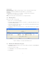
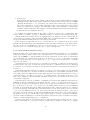
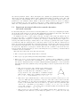
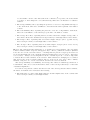
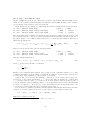
6. You should see a screen like that shown in Figure 1
Figure 1: Siena Data Entry Screen
7. If you do not see this screen, navigate in MyComputer to your R distribution (probably
somewhere like c:/Program Files/R/R-2.9.0), then move to the bin folder and double click on
RSetReg.exe.
5
8. Then try running siena again.
9. If the initial screen appears correctly, then check your working directory or folder. You need
to have permission to write files in the folder in which you work, and you need the data files
you want to use in the same folder. To do this:
(a) Right click on the shortcut, and select Properties. (if somehow you don’t have permission to do this, try copying the shortcut and pasting to create another with fewer
restrictions.) In the Start in: field type the name of the directory in which you wish to
work i.e. a directory in which you can both read and write files Then click OK.
(b) To run the examples, put the session file and the two data files in the chosen directory
before starting siena.
(c) To use your own data, put that data in the chosen directory before starting siena.
2.2
Using the graphical user interface from Mac or Linux
1. Install R (version 2.9.0 or greater) as appropriate for your computer.
2. Within R, type
install.packages(”RSiena”)
3. Navigate to the directory RSiena package, (which you can find from within R by running
system.file(package=”RSiena”)) and find a file called sienascript. Run this to produce the
Siena GUI screen.(You will probably have to change the permissions first (e.g.
chmod u+x sienascript)).
2.3
Running the graphical user interface from within R
The GUI interface can be just as easily be executed from within R, which may be helpful if for
some reason siena.exe does not operate as desired.2 This is done by starting up R and working
with the following commands. Note that R is case-sensitive, so you must use upper and lower case
letters as indicated.
First, set the ‘working directory’ of the R session to the same directory that holds the data
files; for example,
setwd(’C:/SienaTest’)
(Note the forward slash 3 , and the quotes are necessary 4 .) Windows users can use the Change
dir... option on the File menu.
You can use the following commands to make sure the working directory is what you intend
and see which files are included in it:
getwd()
list.files()
Assuming you see the data files, then you can proceed to load the RSiena package, with the
library function:
library(RSiena)
The other packages will be loaded as required, but if you wish to examine them or use other
facilities from them you can load them using:
library(snow)
library(network)
2 We
are grateful to Paul Johnson for supplying these ideas.
can use backward ones but they must be doubled: setwd(’C:\\SienaTest’).
4 Single or double, as long as they match.
3 You
6
library(rlecuyer)
The following way of loading the package will give a review of the functions that it offers:
library(help=RSiena)
After that, you can use the RSiena GUI. It will ‘launch’ out of the R session.
siena01Gui()
You can monitor the R window for error messages – sometimes they are informative.
When you are done, quit R in the polite way:
q()
(Windows users may quit from the File menu or by closing the window.)
2.4
Entering Data.
There are two ways to enter the data.
1. Enter each of your data files using Add.
2. If you have earlier saved the specification of data files, e.g., using Save to file, then you can
use Load new session from File.
3. Check that the Format, Period, Type, are correct, and enter any values which indicate missingness in the Missing Values column.
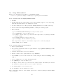
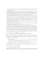
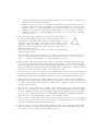
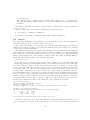
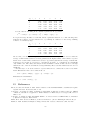
4. A (minimal) complete screen is shown in Figure 2. The details of this screen are explained
in Section 2.6.
Figure 2: Example of a Completed Data Entry Screen
2.5
Running the Estimation Program
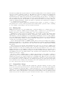
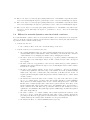
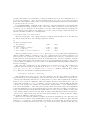
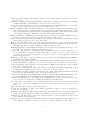
1. Click Apply: you will be prompted to save your work. Then you should see the Model Options
screen shown in Figure 3
2. Select the options you require.
3. Use Edit Effects to choose the effects you wish to include.
4. Click Estimate.
7
Figure 3: Model options screen
5. You should see the SIENA screen of the estimation program.
6. When the program has finished, you should see the results. If not, click Display Results to see
the results. The output file which you will see is stored, with extension .out in the directory
in which you start siena.exe.
7. You may restart your estimation session at a later date using the Continue session from file
on the Data Entry Screen.
8. The restart needs a saved version of the data, effects and model as R objects. This will be
created automatically when you first enter the Model Options Screen, using the default effects
and model. You may save the current version at any time using the Save to file button, and
will be prompted to do so when you leave this screen.
2.6
Details of The Data Entry Screen
Group May be left blank unless you wish to use the multi-group option described in Section 12.1.
Should not contain embedded blanks.
Name Network files or dyadic covariates should use the same name for each file of the set. Other
files should have unique names, a list of space separated ones for constant covariates.
File Name Usually entered by using a file selection box, after clicking Add.
Format Only relevant for networks or dyadic covariates. Can be a matrix or a single Pajek network
(.net).
Period(s) Only relevant for networks and dyadic covariates. All other files cover all the relevant
periods. Indicates the order of the network and dyadic covariate files. Should range from 1
to n within each group.
ActorSet If you have more than one set of nodes, use this column to indicate which is relevant to
each file. Should not contain embedded blanks.
Type Indicate here what type of data the file contains. Options are:
network
behavior
8
constant covariate
changing covariate
constant dyadic covariate
changing dyadic covariate
exogenous event
Selected Yes or No. Only files with Yes will be included in the model.
Missing Values Enter any values which indicate missingness, with spaces between different entries.
Nonzero Codes Enter any values which indicate ties, with spaces between different entries.
If using a file for input, it should have columns with exactly the same names and in exactly the
same order as those of the Data Entry screen, and be of any of the following types:
Extension
.csv
.dat or .prn
.txt
Type
Comma separated
Space delimited
Tab delimited
The root name of this input file will also be the root name of the output file
2.7
Data formats
1. Network and covariate files should be text files with a row for each node. The numbers should
be separated by spaces or tabs.
2. An exogenous events file can be given, indicating change of composition of the network in
the sense that some actors are not part of the network during all the observations. This will
trigger treatment of such change of composition according to Huisman and Snijders (2003).
This file must have one row for each node. Each row should be consist of a set of pairs of
numbers which indicate the periods during which the corresponding actor was present. For
example,
1 3
1.5 3
1 1.4 2.3 3
2.4 3
would describe a network with 4 nodes, and 3 observations. Actor 1 is present all the time,
actor 2 joins at time 1.5, actor 3 leaves and time 1.4 then rejoins at time 2.3, actor 4 joins
at time 2.4. All intervals are treated as closed.
2.8
Continuing the estimation
1. Below you will see some points about how to evaluate the reliability of the results. If the
convergence of the algorithm is not quite satisfactory but not extremely poor, then you can
continue just by Applying the estimation algorithm again.
2. If the parameter estimates obtained are very poor (not in a reasonable range), then it usually
is best to start again, with a simpler model, and from a standardized starting value. The
latter option must be selected in the Model Options screen.
9
2.9
Using SIENA within R
There are two alternatives, depending on your familiarity with R.
Section 2.9.3 presents an example of an R script for getting started with RSiena .
2.9.1
For those who are slightly familiar with R
1. Install R.
2. Install (within R) the package RSiena, and possibly network (required to read Pajek files),
snow and rlecuyer (required to use multiple processors).
3. Set the working directory of R appropriately (setwd() within Ror via a desktop shortcut).
4. Create a session file using siena01Gui() within R, or using an external program.
5. Then, within R,
(a) Use sienaDataCreateFromSession() to create your data objects.
(b) Use getEffects() to create an effects object.
(c) Use fix() to edit the effects object and select the required effects, by altering the Include
column to TRUE.
(d) Use model.create() to create a model object.
(e) Use siena07() to run the estimation procedure.
Basic output will be written to a file. Further output can be obtained by using the
verbose=TRUE option of siena07.
2.9.2
For those fully conversant with R
1. Add the package RSiena
2. Get your network data into matrices or sparse Matrices of type dgTMatrix spMatrix() is useful
to create the latter.
3. Covariate data should be in vectors or matrices.
4. Dyadic covariates can be sparse matrices of type dgTMatrix.
5. Create SIENA objects for each network and covariate, using the functions sienaNet(), coCovar() etc.
6. Create a SIENA data object using SienaDataCreate().
7. Use getEffects() to create an effects object.
8. Use fix() to edit the effects object and select the required effects. Alternatively use normal
R commands to change the effects object: it is just a data frame.
9. Use model.create() to create a model object.
10. Use siena07() to run the estimation procedure.
Basic output will be written to a file. Further output can be obtained by using the verbose=TRUE
option of siena07.
10
2.9.3
An example R script for getting started
The following is an example R script, kindly supplied by Robin Gauthier 5 , which one may use to
get started with RSiena.
#####################################GENERAL###################################
#Lines starting with # are not processed by R but treated as comments.
#R is case sensitive.
#Help within R can be called by typing a question mark and the name of the
#function you need help with. For example ?library loading will bring up a
#file titled "loading and listing of packages".
#Comments are made at the end of commands, or in lines staring with # telling
#R to ignore everything beyond it.
#This session will be using s50 data which are supposed to be
#present in the working directory.
#Note that any command in R is called a function;
#in general the command syntax for calling R’s functions is function(x) where
#function is a saved function and x the name of the object to be operated on.
####################CALLING THE DATA AND PRELIMINARY MANIPULATIONS#############
#The library command loads the packages needed during the session.
library(RSiena)
library(snow) # (these three additional libraies will be loaded
library(network)# automatically if required)
library(rlecuyer)
#The data is named (for example I name it friend.data.w1) so that we can call
#it as an object within R.
#If you read an object straight into R, it will treat it as a
#dataset, which is not what we want because it will generally be harder to work
#with than a matrix (unless you want it to be a dataset (i.e. non-network data).
#R will read in many data formats, these are saved as .dat files, the command
#to read them is read.table if we wished to read a .csv file we would have
#used the read.csv command.
#The pathnames have forward slashes, or double backslashes
#if single backslashes are used, one of the error messages will be:
#
1: ’\R’ is an unrecognized escape in a character string
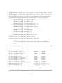
friend.data.w1 <- as.matrix(read.table("s50-network1.dat"))
friend.data.w2 <- as.matrix(read.table("s50-network2.dat"))
drink <- as.matrix(read.table("s50-alcohol.dat"))
#Before we work with the data, we want to be sure it is correct. A simple way
5 slightly
amended by Ruth Ripley
11
#to check that our data is a matrix is the command class()
class(friend.data.w1)
#To check that all the data has been read in, we can use the dim() command. The
#matrix should have the same dimensions as the original data (here, 50 by 50).
dim(friend.data.w1)
#We do the same for the changing covariate that I have labelled "drink". Unlike
#the two matrices it should be 50 by 3 because there are three time points in
#the data, although we will only work with two (we are only working with
#two adjacency matrices.
dim(drink)
####################FROM VECTORS AND MATRICES TO SIENA OBJECTS##################
#model.create creates a basic object which can be used as an argument for Siena07
mymodel <- model.create(findiff=TRUE, fn=simstats0c)
#sienaNet creates a Siena network object from a matrix or array or list of sparse
#matrix of triples.
mynet1 <- sienaNet(array(c(friend.data.w1, friend.data.w2), dim=c(50, 50, 2)))
#varCovar creates a changing covariate object from a matrix. We are only using
#two waves of data, so we only want drinking behavior at time 1 and 2, the
#first two columns of the data. The brackets slice the data into the first two
#columns while the comma indicates that R should read all of the rows.
myvarCovar <- varCovar(drink[,1:2])
#(RSiena should now drop an unnecessary final column automatically.)
#sienaDataCreate creates a Siena data object from input networks,
#covariates and composition change objects.
mydata <- sienaDataCreate(mynet1,myvarCovar)
#getEffects creates a dataframe of effects
myeff <- getEffects(mydata)
#fix calls a data editor, so we can manually edit the effects as in the Gui
fix(myeff)
#Alternatively we can edit the dataframe directly using more data slicing
12
#this command is another way to set "include" to TRUE or FALSE. TRUE or FALSE
#will always be located at the 9th column, but not always at the 11th row as we
#add or remove rate parameters depending on the model. In general the advantage
#of this method is that we can save the last parameters and rerun the model
#later without opening the editor. (Saving can now be done in the GUI).
#myeff[11,9]=TRUE
#myeff[15,9]=TRUE
#myeff[17,9]=TRUE
#myeff[27,9]=TRUE
#myeff[31,9]=TRUE
#myeff[34,9]=TRUE
#myeff[36,9]=TRUE
#myeff[46,9]=TRUE
#myeff[48,9]=TRUE
#myeff[50,9]=TRUE
#myeff[52,9]=TRUE
#myeff[54,9]=TRUE
#myeff[62,9]=TRUE
#(Alternatively use
#transitive triples
#3 cycles
#transitive ties
#indegree popularity
#outdegree popularity
#indegree based activity
#outdegree based activity
#indegree-indegree assortivity
#drinking alter
#drinking alter (squared)
#drinking ego
#drinking similarity
#drinking alter by ego
#myeff[62,’include’]=TRUE)
#siena07 actually fits the specified model to the data
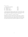
ans <- siena07(mymodel, data=mydata, effects=myeff, batch=TRUE)
ans
###############################################################################
#Rates and standard errors
#1 rate basic rate parameter mynet1
#2 eval outdegree (density)
#3 eval reciprocity
#4 eval transitive triplets
#5 eval 3-cycles
#6 eval transitive ties
#7 eval indegree - popularity
#8 eval outdegree - popularity
#9 eval indegree - activity
#10 eval outdegree - activity
#11 eval in-in degree^(1/2) assortativity
#12 eval myvarCovar alter
#13 eval myvarCovar ego
#14 eval myvarCovar similarity
7.19745
-1.64754
2.09008
0.27810
0.50407
0.63643
0.04709
-0.26251
-0.17380
-0.06880
0.03142
-0.08973
0.03142
1.10065
(
(
(
(
(
(
(
(
(
(
(
(
(
(
1.46778 )
0.21366 )
0.38726 )
0.16612 )
0.37948 )
0.23843 )
0.02693 )
0.66212 )
0.01324 )
0.06258 )
0.90979 )
0.13641 )
0.10044 )
0.72948 )
#The function summary(ans) will give the summary statistics.
###############################################################################
13
2.10
Outline of estimation procedure
SIENA estimates parameters by the following procedure:
1. Certain statistics are chosen that should reflect the parameter values;
the finally obtained parameters should be such that the expected values of the statistics are
equal to the observed values.
Expected values are approximated as the averages over a lot of simulated networks.
Observed values are calculated from the data set. These are also called the target values.
2. To find these parameter values, an iterative stochastic simulation algorithm is applied.
This works as follows:
(a) In Phase 1, the sensitivity of the statistics to the parameters is roughly determined.
(b) In Phase 2, provisional parameter values are updated:
this is done by simulating a network according to the provisional parameter values,
calculating the statistics and the deviations between these simulated statistics and the
target values, and making a little change (the ‘update’) in the parameter values that
hopefully goes into the right direction.
(Only a ‘hopefully’ good update is possible, because the simulated network is only a
random draw from the distribution of networks, and not the expected value itself.)
(c) In Phase 3, the final result of Phase 2 is used, and it is checked if the average statistics
of many simulated networks are indeed close to the target values. This is reflected in
the so-called t statistics for deviations from targets.
2.11
Steps for looking at results: Executing SIENA.
1. Look at the start of the output file for general data description (degrees, etc.), to check your
data input.
2. When parameters have been estimated, first look at the t ratios for deviations from
targets. These are good if they are all smaller than 0.1 in absolute value, and reasonably
good if they are all smaller than 0.2.
We say that the algorithm has converged if they are all smaller than 0.1 in absolute value,
and that it has nearly converged if they are all smaller than 0.2.
These bounds are indications only, and may be taken with a grain of salt.
3. The Initial value of gain parameter determines the step sizes in the parameter updates in the
iterative algorithm. A too low value implies that it takes very long to attain a reasonable
parameter estimate when starting from an initial parameter value that is far from the ‘true’
parameter estimate. A too high value implies that the algorithm will be unstable, and may
be thrown off course into a region of unreasonable (e.g., hopelessly large) parameter values.
It usually is unnecessary to change this.
4. If all this is of no avail, then the conclusion may be that the model specification is incorrect
for the given data set.
5. Further help in interpreting output is in Section 6.2 of this manual.
14
2.12
Giving references
When using SIENA, it is appreciated that you refer to this manual and to one or more relevant
references of the methods implemented in the program. The reference to this manual is the
following.
Ripley, Ruth, and Snijders, Tom A.B. 2009. Manual for SIENA version 4.0 (provisional version, July 6, 2009). Oxford: University of Oxford, Department of Statistics; Nuffield College.
http://www.stats.ox.ac.uk/siena/
A basic reference for the network dynamics model is Snijders (2001) or Snijders (2005). Basic
references for the model of network-behavior co-evolution are Snijders, Steglich, and Schweinberger
(2007) and Steglich, Snijders, and Pearson (2009).
More specific references are Schweinberger (2005) for the score-type goodness of fit tests and
Schweinberger and Snijders (2007) for the calculation of standard errors of the Method of Moments
estimators .
A tutorial is Snijders, van de Bunt, and Steglich (2009).
15
Part II
User’s manual
3
Parts of the program
The operation of the SIENA program is comprised of four main parts:
1. input of basic data description,
2. model specification,
3. estimation of parameter values using stochastic simulation,
4. simulation of the model with given and fixed parameter values.
The normal operation is to start with data input, then specify a model and estimate its parameters, and then continue with new model specifications followed by estimation or simulation.
For the comparison of (nested) models, statistical tests can be carried out.
The main output is written to a text file named pname.out, where pname is the root name of
the file specifying the data files (if any).
16
4
Input data
The main statistical method implemented in SIENA is for the analysis of repeated measures of
social networks, and requires network data collected at two or more time points. It is possible
to include changing actor variables (representing behavior, attitudes, outcomes, etc.) which also
develop in a dynamic process, together with the social networks. As repeated measures data on
social networks, at the very least, two or more data files with digraphs are required: the observed
networks, one for each time point. The number of time points is denoted M .
In addition, various kinds of variables are allowed:
1. actor-bound or individual variables, also called actor attributes, which can be symbolized as
vi for each actor i; these can be constant over time or changing;
the changing individual variables can be dependent variables (changing dynamically in mutual dependence with the changing network) or independent variables (exogenously changing
variables; then they are also called individual covariates).
2. dyadic covariates, which can be symbolized as wij for each ordered pair of actors (i, j); these
likewise can be constant over time or changing.
All variables must be available in ASCII (‘raw text’) data files, described in detail below. It is
best to use the ‘classical’ type of filenames, without embedded blanks and not containing special
characters. These files, the names of the corresponding variables, and the coding of missing data,
must be made available to SIENA.
Names of variables must be composed of at most 12 characters. This is because they are used
as parts of the names of effects which can be included in the model, and the effect names should
not be too long.
4.1
Digraph data files
Each digraph must be contained in a separate input file. Two data formats are allowed currently.
For large number of nodes (say, larger than 100), the Pajek format is preferable to the adjacency
matrix format. For more than a few hundred nodes,
1. Adjacency matrices.
The first is an adjacency matrix, i.e., n lines each with n integer numbers, separated by
blanks or tabs, each line ended by a hard return. The diagonal values are meaningless but
must be present.
Although this section talks only about digraphs (directed graphs), it is also possible that all
observed adjacency matrices are symmetric. This will be automatically detected by SIENA,
and the program will then utilize methods for non-directed networks.
The data matrices for the digraphs must be coded in the sense that their values are converted
by the program to the 0 and 1 entries in the adjacency matrix. A set of code numbers is
required for each digraph data matrix; these codes are regarded as the numbers representing
a present arc in the digraph, i.e., a 1 entry in the adjacency matrix; all other numbers will
be regarded as 0 entries in the adjacency matrix. Of course, there must be at least one such
code number. All code numbers must be in the range from 0 to 9, except for structurally
determined values (see below).
This implies that if the data are already in 0-1 format, the single code number 1 must be
given. As another example, if the data matrix contains values 1 to 5 and only the values 4
and 5 are to be interpreted as present arcs, then the code numbers 4 and 5 must be given.
17
2. Pajek format.
If the digraph data file has extension name .net, then the program assumes that the data file
has Pajek format. The format required differs from that in the previous versions of SIENA
. The file should relate to one observation only, and should contain a list of vertices (using
the keyword *Vertices, together with (currently) a list of arcs, using the keyword *Arcs
followed by data lines according to the Pajek rules. These keywords must be in lines that
contain no further characters. An example of such input files is given in the s50 data set that
is distributed in the examples directory.
Code numbers for missing numbers also must be indicated – in the case of either input data
format. These codes must, of course, be different from the code numbers representing present arcs.
Although this section talks only about digraphs (directed graphs), it is also possible that all
observed ties (for all time points) are mutual. This will be automatically detected by SIENA, and
the program will then utilize methods for non-directed networks.
If the data set is such that it is never observed that ties are terminated, then the network
dynamics is automatically specified internally in such a way that termination of ties is impossible.
(In other words, in the simulations of the actor-based model the actors have only the option to
create new ties or to retain the status quo, not to delete existing ties.)
4.1.1
Structurally determined values
It is allowed that some of the values in the digraph are structurally determined, i.e., deterministic
rather than random. This is analogous to the phenomenon of ‘structural zeros’ in contingency
tables, but in SIENA not only structural zeros but also structural ones are allowed. A structural
zero means that it is certain that there is no tie from actor i to actor j; a structural one means
that it is certain that there is a tie. This can be, e.g., because the tie is impossible or formally
imposed, respectively.
Structural zeros provide an easy way to deal with actors leaving or joining the network between
the start and the end of the observations. Another way (more complicated but it gives possibilities
to represent actors entering or leaving at specified moments between observations) is described in
Section 4.7.
Structurally determined values are defined by reserved codes in the input data: the value 10
indicates a structural zero, the value 11 indicates a structural one. Structurally determined values
can be different for the different time points. (The diagonal of the data matrix always is composed
of structural zeros, but this does not have to be indicated in the data matrix by special codes.)
The correct definition of the structurally determined values can be checked from the brief report
of this in the output file.
Structural zeros offer the possibility of analyzing several networks simultaneously under the
assumption that the parameters are identical. Another option to do this is given in Section 12.
E.g., if there are three networks with 12, 20 and 15 actors, respectively, then these can be integrated
into one network of 12 + 20 + 15 = 47 actors, by specifying that ties between actors in different
networks are structurally impossible. This means that the three adjacency matrices are combined
in one 47×47 data file, with values 10 for all entries that refer to the tie from an actor in one network
to an actor in a different network. In other words, the adjacency matrices will be composed of
three diagonal blocks, and the off-diagonal blocks will have all entries equal to 10. In this example,
the number of actors per network (12 to 20) is rather small to obtain good parameter estimates,
but if the additional assumption of identical parameter values for the three networks is reasonable,
then the combined analysis may give good estimates.
In such a case where K networks (in the preceding paragraph, the example had K = 3) are
combined artificially into one bigger network, it will often be helpful to define K − 1 dummy
18
variables at the actor level to distinguish between the K components. These dummy variables can
be given effects in the rate function and in the evaluation function (for “ego”), which then will
represent that the rate of change and the out-degree effect are different between the components,
while all other parameters are the same.
It will be automatically discovered by SIENA when functions depend only on these components
defined by structural zeros, between which tie values are not allowed. For such variables, only
the ego effects are defined and not the other effects defined for the regular actor covariates and
described in Section 5.2. This is because the other effects then are meaningless. If at least one
case is missing (i.e., has the missing value data code for this covariate), then the other covariate
effects are made available.
When SIENA simulates networks including some structurally determined values, if these values
are constant across all observations then the simulated tie values are likewise constant. If the
structural fixation varies over time, the situation is more complicated. Consider the case of two
sim
be the simulated value at the end of the
consecutive observations m and m + 1, and let Xij
period from tm to tm+1 . If the tie variable Xij is structurally fixed at time tm at a value xij (tm ),
sim
then Xij
also is equal to xij (tm ), independently of whether this tie variable is structurally fixed
at time tm+1 at the same or a different value or not at all. This is the direct consequence of the
structural fixation. On the other hand, the following rule is also used. If Xij is not structurally
fixed at time tm but it is structurally fixed at time tm+1 at some value xij (tm+1 ), then in the
course of the simulation process from tm to tm+1 this tie variable can be changed as part of the
process in the usual way, but after the simulation is over and before the statistics are calculated it
will be fixed to the value xij (tm+1 ).
The target values for the algorithm of the Method of Moments estimation procedure are calculated for all observed digraphs x(tm+1 ). However, for tie variables Xij that are structurally fixed
at time tm , the observed value xij (tm+1 ) is replaced by the structurally fixed value xij (tm ). This
gives the best possible correspondence between target values and simulated values in the case of
changing structural fixation.
4.2
Dyadic covariates
As the digraph data, also each measurement of a dyadic covariate must be contained in a separate
input file with a square data matrix, i.e., n lines each with n integer numbers, separated by blanks
or tabs, each line ended by a hard return. The diagonal values are meaningless but must be present.
Pajek input format is currently not possible for dyadic covariates.
A distinction is made between constant and changing dyadic covariates, where change refers to
changes over time. Each constant covariate has one value for each pair of actors, which is valid
for all observation moments, and has the role of an independent variable. Changing covariates, on
the other hand, have one such value for each period between measurement points. If there are M
waves of network data, this covers M − 1 periods, and accordingly, for specifying a single changing
dyadic covariate, M − 1 data files with covariate matrices are needed.
The mean is always subtracted from the covariates. See the section on Centering.
4.3
Individual covariates
Individual (i.e., actor-bound) variables can be combined in one or more files. If there are k variables
in one file, then this data file must contain n lines, with on each line k numbers which all are read
as real numbers (i.e., a decimal point is allowed). The numbers in the file must be separated by
blanks and each line must be ended by a hard return. There must not be blank lines after the last
data line.
19
Also here, a distinction is made between constant and changing actor variables. Each constant
actor covariate has one value per actor valid for all observation moments, and has the role of an
independent variable.
Changing variables can change between observation moments. They can have the role of dependent variables (changing dynamically in mutual dependence with the changing network) or
of independent variables; in the latter case, they are also called ‘changing individual covariates’.
Dependent variables are treated in the section below, this section is about individual variables in
the role of independent variables – then they are also called individual covariates.
When changing individual variables have the role of independent variables, they are assumed
to have constant values from one observation moment to the next. If observation moments for
the network are t1 , t2 , ..., tM , then the changing covariates should refer to the M − 1 moments
t1 through tM −1 , and the m-th value of the changing covariates is assumed to be valid for the
period from moment tm to moment tm+1 . The value at tM , the last moment, does not play a
role. Changing covariates, as independent variables, are meaningful only if there are 3 or more
observation moments, because for 2 observation moments the distinction between constant and
changing covariates is not meaningful.
Each changing individual covariate must be given in one file, containing k = M − 1 columns
that correspond to the M − 1 periods between observations. It is not a problem if there is an M ’th
column in the file, but it will not be read.
The mean is always subtracted from the covariates. See the section on Centering.
When an actor covariate is constant within waves, or constant within components separated
by structural zeros (which means that ties between such components are not allowed), then only
the ego effect of the actor covariate is made available. This is because the other effects then are
meaningless. This may cause problems for combining several data sets in a meta-analysis (see
Section 12). If at least one case is missing (i.e., has the missing value data code), then the other
covariate effects are made available. When analysing multiple data sets in parallel, for which the
same set of effects is desired to be included it is therefore advisable to give data sets in which a
given covariate has the same value for all actors one missing value in this covariate; purely to make
the total list of effects independent of the observed data.
4.4
Interactions and dyadic transformations of covariates
For actor covariates, two kinds of transformations to dyadic covariates are made internally in
SIENA. Denote the actor covariate by vi , and the two actors in the dyad by i and j. Suppose that
the range of vi (i.e., the difference between the highest and the lowest values) is given by rV . The
two transformations are the following:
1. dyadic similarity, defined by 1− |vi −vj |/rV , and centered so the the mean of this similarity
variable becomes 0;
note that before centering, the similarity variable is 1 if the two actors have the same value,
and 0 if one has the highest and the other the lowest possible value;
2. same V , defined by 1 if vi = vj , and 0 otherwise (not centered) (V is the name of the
variable). This can also be referred to as dyadic identity with respect to V .
Dyadic similarity is relevant for variables that can be treated as interval-level variables; dyadic
identity is relevant for categorical variables.
4.5
Dependent action variables
SIENA also allows dependent action variables, also called dependent behavior variables. This can be
used in studies of the co-evolution of networks and behavior, as described in Snijders, Steglich, and
20
Schweinberger (2007) and Steglich, Snijders, and Pearson (2009). These action variables represent
the actors’ behavior, attitudes, beliefs, etc. The difference between dependent action variables and
changing actor covariates is that the latter change exogenously, i.e., according to mechanisms not
included in the model, while the dependent action variables change endogenously, i.e., depending on
their own values and on the changing network. In the current implementation only one dependent
network variable is allowed, but the number of dependent action variable can be larger than one.
Unlike the changing individual covariates, the values of dependent action variables are not assumed
to be constant between observations.
Dependent action variables must have nonnegative integer values; e.g., 0 and 1, or a range of
integers like 0,1,2 or 1,2,3,4,5. Each dependent action variable must be given in one file, containing
k = M columns, corresponding to the M observation moments.
4.6
Missing data
SIENA allows that there are some missing data on network variables, on covariates, and on dependent action variables. Missing data in changing dyadic covariates are not yet implemented.
Missing data must be indicated by missing data codes, not by blanks in the data set.
Missingness of data is treated as non-informative. One should be aware that having many
missing data can seriously impair the analyses: technically, because estimation will be less stable;
substantively, because the assumption of non-informative missingness often is not quite justified.
Up to 10% missing data will usually not give many difficulties or distortions, provided missingness
is indeed non-informative. When one has more than 20% missing data on any variable, however,
one may expect problems in getting good estimates.
In the current implementation of SIENA, missing data are treated in a simple way, trying to
minimize their influence on the estimation results. This method is further explained in Huisman
and Steglich (2008), where comparisons are also made with other ways of dealings with the missing
information.
The basic idea is the following. The simulations are carried out over all actors. Missing data
are treated separately for each period between two consecutive observations of the network. In the
initial observation for each period, missing entries in the adjacency matrix are set to 0, i.e., it is
assumed that there is no tie. Missing covariate data as well as missing entries on dependent action
variables are replaced by the variable’s average score at this observation moment. In the course of
the simulations, however, the adjusted values of the dependent action variables and of the network
variables are allowed to change.
In order to ensure a minimal impact of missing data treatment on the results of parameter
estimation (method of moments estimation) and/or simulation runs, the calculation of the target
statistics used for these procedures is restricted to non-missing data. When for an actor in a given
period, any variable is missing that is required for calculating a contribution to such a statistic, this
actor in this period does not contribute to the statistic in question. For network and dependent
action variables, an actor must provide valid data both at the beginning and at the end of a period
for being counted in the respective target statistics.
4.7
Composition change
SIENA can also be used to analyze networks of which the composition changes over time, because
actors join or leave the network between the observations. This can be done in two ways: using the
method of Huisman and Snijders (2003), or using structural zeros. (For the maximum likelihood
estimation option, the Huisman-Snijders method is not implemented, and only the structural zeros
method can be used.) Structural zeros can specified for all elements of the tie variables toward
and from actors who are absent at a given observation moment. How to do this is described in
21
subsection 4.1.1. This is straightforward and not further explained here. This subsection explains
the method of Huisman and Snijders (2003), which uses the information about composition change
in a sightly more efficient way.
For this case, a data file is needed in which the times of composition change are given. For
networks with constant composition (no entering or leaving actors), this file is omitted and the
current subsection can be disregarded.
Network composition change, due to actors joining or leaving the network, is handled separately
from the treatment of missing data. The digraph data files must contain all actors who are part of
the network at any observation time (denoted by n) and each actor must be given a separate (and
fixed) line in these files, even for observation times where the actor is not a part of the network
(e.g., when the actor did not yet join or the actor already left the network). In other words, the
adjacency matrix for each observation time has dimensions n × n.
At these times, where the actor is not in the network, the entries of the adjacency matrix can
be specified in two ways. First as missing values using missing value code(s). In the estimation
procedure, these missing values of the joiners before they joined the network are regarded as 0
entries, and the missing entries of the leavers after they left the network are fixed at the last
observed values. This is different from the regular missing data treatment. Note that in the
initial data description the missing values of the joiners and leavers are treated as regular missing
observations. This will increase the fractions of missing data and influence the initial values of the
density parameter.
A second way is by giving the entries a regular observed code, representing the absence or
presence of an arc in the digraph (as if the actor was a part of the network). In this case, additional
information on relations between joiners and other actors in the network before joining, or leavers
and other actors after leaving can be used if available. Note that this second option of specifying
entries always supersedes the first specification: if a valid code number is specified this will always
be used.
For joiners and leavers, crucial information is contained in the times they join or leave the
network (i.e., the times of composition change), which must be presented in a separate input file,
the exogenous events file described in Section 2.7.
4.8
Centering
Individual as well as dyadic covariates are centered by the program in the following way.
For individual covariates, the mean value is subtracted immediately after reading the variables.
For the changing covariates, this is the global mean (averaged over all periods). The values of
these subtracted means are reported in the output.
For the dyadic covariates and the similarity variables derived from the individual covariates, the
grand mean is calculated, stored, and subtracted during the program calculations. (Thus, dyadic
covariates are treated by the program differently than individual covariates in the sense that the
mean is subtracted at a different moment, but the effect is exactly the same.)
The formula for balance is a kind of dissimilarity between rows of the adjacency matrix. The
mean dissimilarity is subtracted in this formula and also reported in the output. This mean
dissimilarity is calculated by a formula given in Section 13.
22
5
Model specification
After defining the data, the next step is to specify a model.
The model specification consists of a selection of ‘effects’ for the evolution of each dependent
variable (network or behavior).
For the longitudinal case, three types of effects are distinguished (see Snijders, 2001; Snijders,
van de Bunt, and Steglich, 2009):
• rate function effects
The rate function models the speed by which the dependent variable changes; more precisely:
the speed by which each network actor gets an opportunity for changing her score on the
dependent variable.
Advice: in most cases, start modeling with a constant rate function without additional rate
function effects. Constant rate functions are selected by exclusively checking the ‘basic rate
parameter’ (for network evolution) and the main rate effects (for behavioral evolution) on
the model specification screen. (When there are important size or activity differences between
actors, it is possible that different advice must be given, and it may be necessary to let the
rate function depend on the individual covariate that indicates this size; or on the out-degree.)
• evaluation function effects
The evaluation function6 models the network actors’ satisfaction with their local network
neighborhood configuration. It is assumed that actors change their scores on the dependent
variable such that they improve their total satisfaction – with a random element to represent
the limited predictability of behavior. In contrast to the endowment function (described
below), the evaluation function evaluates only the local network neighborhood configuration
that results from the change under consideration. In most applications, the evaluation function will be the main focus of model selection.
The network evaluation function normally should always contain the ‘density’, or ‘out-degree’
effect, to account for the observed density. For directed networks, it mostly is also advisable
to include the reciprocity effect, this being one of the most fundamental network effects. Likewise, behavior evaluation functions should normally always contain the shape parameter, to
account for the observed prevalence of the behavior, and (unless the behavior is dichotomous)
the quadratic shape effect, to account more precisely for the distribution of the behavior.
• endowment function effects
The endowment function7 is an extension of the evaluation function that allows to distinguish
between new and old network ties (when evaluating possible network changes) and between
increasing or decreasing behavioral scores (when evaluating possible behavioral changes).
The function models the loss of satisfaction incurred when existing network ties are dissolved
or when behavioral scores are decreased to a lower value (hence the label ‘endowment’).
For a number of effects, the endowment function is implemented not for the Method of
Moments estimation method, but only for Maximum Likelihood and Bayesian estimation.
This is indicated in Section 13.
Advice: start modeling without any endowment effects, and add them at a later stage. Do
not use endowment effects for behavior unless the behavior variable is dichotomous.
The estimation and simulation procedures of SIENA operate on the basis of the model specification which comprises the set of effects included in the model as described above, together with
6 The
7 The
evaluation function was called objective function in Snijders, 2001.
endowment function is similar to the gratification function in Snijders, 2001.
23
the current parameter values. After data input, the constant rate parameters and the density
effect in the network evaluation function have default initial values, depending on the data. All
other parameter values initially are 0. The estimation process changes the current value of the
parameters to the estimated values. Values of effects not included in the model are not changed
by the estimation process. It is possible for the user to change parameter values and to request
that some of the parameters are fixed in the estimation process at their current value.
5.1
Important structural effects for network dynamics:
one-mode networks
For the structural part of the model for network dynamics, for one-mode (or unipartite) networks,
the most important effects are as follows. The mathematical formulae for these and other effects
are given in Section 13. Here we give a more qualitative description.
A default model choice could consist of (1) the out-degree and reciprocity effects; (2) one
network closure effect, e.g. transitive triplets or transitive ties; the 3-cycles effect; (3) the in-degree
popularity effect (raw or square root version); the out-degree activity effect (raw or square root
version); and either the in-degree activity effect or the out-degree popularity effect (raw or square
root function). The two effects (1) are so basic they cannot be left out. The two effects selected
under (2) represent the dynamics in local (triadic) structure; and the three effects selected under
(3) represent the dynamics in in- and out-degrees (the first for the dispersion of in-degrees, the
second for the dispersion of out-degrees, and the third for the covariance between in- and outdegrees) and also should offer some protection, albeit imperfect, for potential ego- and alter-effects
of omitted actor-level variables.
The basic list of these and other effects is as follows.
1. The out-degree effect which always must be included.
2. The reciprocity effect which practically always must be included.
3. There is a choice of four network closure effects. Usually it will be sufficient to express
the tendency to network closure by including one or two of these. They can be selected by
theoretical considerations and/or by their empirical statistical significance. Some researchers
may find the last effect (distances two) less appealing because it expresses network closure
inversely.
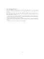
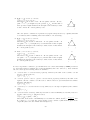
a. The transitive triplets effect, which is the classical representation of network closure by the number of transitive
triplets. For this effect the contribution of the tie i → j
is proportional to the total number of transitive triplets
that it forms – which can be transitive triplets of the type
{i → j → h; i → h} as well as {i → h → j; i → j};
h
•
.. ..
......... ...
... ....
...
...
...
...
..
...
...
...
.
.
...
...
.
....
..
.........
.
..
...
....................................................
•
•
i
j
b. The balance effect, which may also be called structural equivalence with respect to outgoing ties. This expresses a preference of actors to have ties to those other actors who
have a similar set of outgoing ties as themselves. Whereas the transitive triplets effect
focuses on how many same choices are made by ego (the focal actor) and alter (the
other actor) — the number of h for which i → h and j → h, i.e., xih = xjh = 1 where
i is ego and j is alter — , the balance effect considers in addition how many the same
non-choices are made — xih = xjh = 0.
c. The transitive ties effect is similar to the transitive triplets effect, but instead of considering for each other actor j how many two-paths i → h → j there are, it is only
24
considered whether there is at least one such indirect connection. Thus, one indirect tie
suffices for the network embeddedness.
d. The number of actors at distance two effect expresses network closure inversely: stronger
network closure (when the total number of ties is fixed) will lead to fewer geodesic
distances equal to 2. When this effect has a negative parameter, actors will have a
preference for having few others at a geodesic distance of 2 (given their out-degree,
which is the number of others at distance 1); this is one of the ways for expressing
network closure.
4. The three-cycles effect, which can be regarded as generalized reciprocity (in an exchange interpretation of the network) but also as
the opposite of hierarchy (in a partial order interpretation of the
network). A negative three-cycles effect, together with a positive
transitive triplets or transitive ties effect, may be interpreted as a
tendency toward local hierarchy. The three-cycles effect also contributes to network closure.
In a non-directed network, the three-cycles effect is identical to the
transitive triplets effect.
h
•
. ....
... ..........
...
...
..
...
.
.
.
...
...
...
...
...
.
.
...
.
.
...
...........
.
...
..
....................................................
•
•
i
j
5. Another triadic effect is the betweenness effect, which represents brokerage: the tendency for
actors to position themselves between not directly connected others, i.e., a preference of i for
ties i → j to those j for which there are many h with h → i and h 6→ j.
J
The following eight degree-related effects may be important especially for networks where
degrees are theoretically important and represent social status or other features important
for network dynamics; and/or for networks with high dispersion in in- or out-degrees (which
may be an empirical reflection of the theoretical importance of the degrees). Include them if
there are theoretical reasons for doing so, but only in such cases.
6. The in-degree popularity effect (again, with or without ‘sqrt’, with the same considerations
applying) reflects tendencies to dispersion in in-degrees of the actors; or, tendencies for actors
with high in-degrees to attract extra incoming ties ‘because’ of their high current in-degrees.
7. The out-degree popularity effect (again, with or without ‘sqrt’, with the same considerations
applying) reflects tendencies for actors with high out-degrees to attract extra incoming ties
‘because’ of their high current out-degrees. This leads to a higher correlation between indegrees and out-degrees.
8. The in-degree activity effect (with or without ‘sqrt’) reflects tendencies for actors with high
in-degrees to send out extra outgoing ties ‘because’ of their high current in-degrees. This
leads to a higher correlation between in-degrees and out-degrees. The in-degree popularity
and out-degree activity effects are not distinguishable in Method of Moments estimation;
then the choice between them must be made on theoretical grounds.
9. The out-degree activity effect (with or without ‘sqrt’) reflects tendencies for actors with high
out-degrees to send out extra outgoing ties ‘because’ of their high current out-degrees. This
also leads to dispersion in out-degrees of the actors.
10. The in-in degree assortativity effect (where parameter 2 is the same as the sqrt version, while
parameter 1 is the non-sqrt version) reflects tendencies for actors with high in-degrees to
preferably be tied to other actors with high in-degrees.
25
11. The in-out degree assortativity effect (with parameters 2 or 1 in similar roles) reflects tendencies for actors with high in-degrees to preferably be tied to other actors with high out-degrees.
12. The out-in degree assortativity effect (with parameters 2 or 1 in similar roles) reflects tendencies for actors with high out-degrees to preferably be tied to other actors with high in-degrees.
13. The out-out degree assortativity effect (with parameters 2 or 1 in similar roles) reflects tendencies for actors with high out-degrees to preferably be tied to other actors with high
out-degrees.
5.2
Effects for network dynamics associated with covariates
For each individual covariate, there are several effects which can be included in a model specification, both in the network evolution part and in the behavioral evolution part (should there be
dependent behavior variables in the data).
• network rate function
1. the covariate’s effect on the rate of network change of the actor;
• network evaluation and endowment functions
1. the covariate-similarity effect; a positive parameter implies that actors prefer ties to others with similar values on this variable – thus contributing to the network-autocorrelation
of this variable not by changing the variable but by changing the network;
2. the effect on the actor’s activity (covariate-ego); a positive parameter will imply the
tendency that actors with higher values on this covariate increase their out-degrees
more rapidly;
3. the effect on the actor’s popularity to other actors (covariate-alter); a positive parameter
will imply the tendency that the in-degrees of actors with higher values on this covariate
increase more rapidly;
4. the effect of the squared variable on the actor’s popularity to other actors (squared
covariate-alter) (included only if the range of the variable is at least 2). This normally
makes sense only if the covariate-alter effect itself also is included in the model. A
negative parameter implies a unimodal preference function with respect to alters’ values
on this covariate;
5. the interaction between the value of the covariate of ego and of the other actor (covariate ego × covariate alter); a positive effect here means, just like a positive similarity
effect, that actors with a higher value on the covariate will prefer ties to others who
likewise have a relatively high value; when used together with the alter effect of the
squared variable this effect is quite analogous to the similarity effect, and for dichotomous covariates, in models where the ego and alter effects are also included, it even is
equivalent to the similarity effect (although expressed differently), and then the squared
alter effect is superfluous;
6. the ‘same covariate’, or covariate identity, effect, which expresses the tendency of the
actors to be tied to others with exactly the same value on the covariate; whereas the
preceding four effects are appropriate for interval scaled covariates (and mostly also for
ordinal variables), the identity effect is suitable for categorical variables;
7. the interaction effect of covariate-similarity with reciprocity;
26
8. the effect of the covariate of those to whom the actor is indirectly connected, i.e., through
one intermediary but not with a direct tie; this value-at-a-distance can represent effects
of indirectly accessed social capital.
The usual order of importance of these covariate effects on network evolution is: evaluation effects
are most important, followed by endowment and rate effects. Inside the group of evaluation effects,
it is the covariate-similarity effect that is most important, followed by the effects of covariate-ego
and covariate-alter.
When the network dynamics is not smooth over the observation waves — meaning that the
pattern of ties created and terminated, as reported in the initial part of the output file under the
heading Initial data description – Change in networks – Tie changes between subsequent observations, is very irregular across the observation periods — it can be important to include effects of
time variables on the network. Time variables are changing actor covariates that depend only on
the observation number and not on the actors. E.g., they could be dummy variables, being 1 for
one or some observations, and 0 for the other observations.
For actor covariates that are constant within observation waves, or – in the case that there are
structurally determined values – constant within connected components, only the ego effects are
defined, because only those effects are meaningful. This exclusion of the alter, similarity and other
effects for such actor variables applies only to variables without any missing values.
For each dyadic covariate, the following network evaluation effects can be included in the model
for network evolution:
• network evaluation and endowment functions
1. main effect of the dyadic covariate;
2. the interaction effect of the dyadic covariate with reciprocity.
The main evaluation effect is usually the most important. In the current version of SIENA, there
are no effects of dyadic covariates on behavioral evolution.
5.3
Effects on behavior evolution
For models with one or more dependent behavior variables, i.e., models for the co-evolution of
networks and behavior, the most important effects for the behavior dynamics are the following; see
Steglich, Snijders, and Pearson (2009). In these descriptions, with the ‘alters’ of an actor we refer
to the other actors to whom the focal actor has an outgoing tie. The dependent behavior variable
is referred to as Z.
1. The shape effect, expressing the basic drive toward high values on Z. A zero value for the
shape will imply a drift toward the midpoint of the range of the behavior variable.
2. The effect of the behavior Z on itself, or quadratic shape effect, which is relevant only if the
number of behavioral categories is 3 or more. This can be interpreted as giving a quadratic
preference function for the behavior. When the coefficient for the shape effect is β1Z and for
the effect of Z on itself, or quadratic shape effect, is β2Z , then the contributions of these two
effects are jointly β1Z (zi − z̄) + β2Z (zi − z̄)2 . With a negative coefficient β2Z , this is a unimodal
preference function, with the maximum attained for zi = z̄ − 2 β1Z /β2Z . (Of course additional
effects will lead to a different picture; but as long as the additional effects are linear in zi –
which is not the case for similarity effects! –, this will change the location of the maximum
but not the unimodal shape of the function.) This can also be regarded as negative feedback,
or a self-correcting mechanism: when zi increases, the further push toward higher values of
zi will become smaller and when zi decreases, the further push toward lower values of zi will
27
become smaller. On the other hand, when the coefficient β2Z is positive, the feedback will
be positive, so that changes in zi are self-reinforcing. This can be an indication of addictive
behavior.
3. The average similarity effect, expressing the preference of actors to being similar with respect
to Z to their alters, where the total influence of the alters is the same regardless of the number
of alters.
4. The total similarity effect, expressing the preference of actors to being similar to their alters,
where the total influence of the alters is proportional to the number of alters.
5. The average alter effect, expressing that actors whose alters have a higher average value of
the behavior Z, also have themselves a stronger tendency toward high values on the behavior.
6. The indegree effect, expressing that actors with a higher indegree (more ‘popular’ actors)
have a stronger tendency toward high values on the behavior.
7. The outdegree effect, expressing that actors with a higher outdegree (more ‘active’ actors)
have a stronger tendency toward high values on the behavior.
Effects 1 and 2 will practically always have to be included as control variables. (For dependent
behavior variables with 2 categories, this applies only to effect 1.) When the behavior dynamics
is not smooth over the observation waves — meaning that the pattern of steps up and down, as
reported in the initial part of the output file under the heading Initial data description – Dependent
actor variables – Changes, is very irregular across the observation periods — it can be important
to include effects of time variables on the behavior. Time variables are changing actor covariates
that depend only on the observation number and not on the actors. E.g., they could be dummy
variables, being 1 for one or some observations, and 0 for the other observations.
The average similarity, total similarity, and average alter effects are different specifications of
social influence. The choice between them will be made on theoretical grounds and/or on the basis
of statistical significance.
For each actor-dependent covariate as well as for each of the other dependent behavior variables,
the effects on Z which can be included is the following.
1. The main effect: a positive value implies that actors with a higher value on the covariate will
have a stronger tendency toward high Z values.
28
6
Estimation
The model parameters are estimated under the specification given during the model specification
part, using a stochastic approximation algorithm. Only one estimation procedure is currently implemented: the Method of Moments (MoM) (Snijders, 2001; Snijders, Steglich, and Schweinberger,
2007);
In the following, the number of parameters is denoted by p. The algorithm is based on repeated
(and repeated, and repeated...) simulation of the evolution process of the network. These repetitions are called ‘runs’ in the following. The MoM estimation algorithm is based on comparing
the observed network (obtained from the data files) to the hypothetical networks generated in the
simulations.
Note that the estimation algorithm is of a stochastic nature, so the results can vary! This is of
course not what you would like. For well-fitting combinations of data set and model, the estimation
results obtained in different trials will be very similar. It is good to repeat the estimation process
at least once for the models that are to be reported in papers or presentations, to confirm that
what you report is a stable result of the algorithm.
The initial value of the parameters normally is the current value (that is, the value that the
parameters have immediately before you start the estimation process); as an alternative, it is
possible to start instead with a standard initial value. Usually, a sequence of models can be fitted
without problems, each using the previously obtained estimate as the starting point for the new
estimation procedure. Sometimes, however, problems may occur during the estimation process,
which will be indicated by some kind of warning in the output file or by parameter estimates
being outside a reasonably expected range. In such cases the current parameter estimates may be
unsatisfactory, and using them as initial values for the new estimation process might again lead to
difficulties in estimation. Therefore, when the current parameter values are unlikely and also when
they were obtained after a divergent estimation algorithm, it is advisable to start the estimation
algorithm with a standard initial value. The use of standard initial values is one of the model
options. If this has successfully led to a model with convergent parameter estimates and model
fitting is continued, then the option can be reset to the current initial values.
6.1
Algorithm
The estimation algorithm is an implementation of the Robbins-Monro (1951) algorithm, described
in Snijders (2001, 2002), and has three phases:
1. In phase 1, the parameter vector is held constant at its initial value. This phase is for having
a first rough estimate of the matrix of derivatives.
2. Phase 2 consists of several subphases. More subphases means a greater precision. The
default number of subphases is 4. The parameter values change from run to run, reflecting
the deviations between generated and observed values of the statistics. The changes in the
parameter values are smaller in the later subphases.
The program searches for parameter values where these deviations average out to 0. This
is reflected by what is called the ‘quasi-autocorrelations’ in the output screen. These are
averages of products of successively generated deviations between generated and observed
statistics. It is a good sign for the convergence of the process when the quasi-autocorrelations
are negative (or positive but close to 0), because this means the generated values are jumping
around the observed values.
3. In phase 3, the parameter vector is held constant again, now at its final value. This phase is
for estimating the covariance matrix and the matrix of derivatives used for the computation
29
of standard errors.
The default number of runs in phase 3 is 1000. This requires a lot of computing time,
but when the number of phase 3 runs is too low, the standard errors computed are rather
unreliable.
The number of subphases in phase 2, and the number of runs in phase 3, can be changed in
the model options.
The user can break in and modify the estimation process in three ways:
1. it is possible to terminate the estimation;
2. in phase 2, it is possible to terminate phase 2 and continue with phase 3;
6.2
Output
The output file is an ASCII (‘text’) file which can be read by any text editor. It is called pname.out
(recall that pname is the project name defined by the user).
The output is divided into sections indicated by a line @1, subsections indicated by a line @2,
subsubsections indicated by @3, etc. For getting the main structure of the output, it is convenient
to have a look at the @1 marks first.
The primary information in the output of the estimation process consists of the following three
parts. Results are presented here which correspond to Table 2, column “t1 , t3 ” of Snijders (2001).
The results were obtained in an independent repetition of the estimation for this data set and
this model specification; since the repetition was independent, the results are slightly different,
illustrating the stochastic nature of the estimation algorithm.
1. Convergence check
In the first place, a convergence check is given, based on Phase 3 of the algorithm. This check
considers the deviations between simulated values of the statistics and their observed values (the
latter are called the ‘targets’). Ideally, these deviations should be 0. Because of the stochastic
nature of the algorithm, when the process has properly converged the deviations are small but
not exactly equal to 0. The program calculates the averages and standard deviations of the
deviations and combines these in a t-ratio (in this case, average divided by standard deviation).
For longitudinal modeling, convergence is excellent when these t-ratios are less than 0.1 in absolute
value, good when they are less than 0.2, and moderate when they are less than 0.3. For published
results, it is suggested that estimates presented come from runs in which all t-ratios for convergence
are less than 0.1 in absolute value – or nearly so. (These bounds are indications only, and are not
meant as severe limitations.) The corresponding part of the output is the following.
Total of 1954 iterations.
Parameter estimates based on 954 iterations,
basic rate parameter as well as
convergence diagnostics, covariance and derivative matrices based on 1000 iterations.
Information for convergence diagnosis.
Averages, standard deviations, and t-ratios for deviations from targets:
1.
-0.236
7.006
-0.034
2.
0.204
7.059
0.029
3.
-1.592
22.242
-0.072
Good convergence is indicated by the t-ratios being close to zero.
In this case, the t-ratios are -0.034, -0.029, and -0.072, which is less than 0.1 in absolute value,
so the convergence is excellent. In data exploration, if one or more of these t-ratios are larger in
30
absolute value than 0.3, it is advisable to restart the estimation process. For results that are to be
reported, it is advisable to carry out a new estimation when one or more of the t-ratios are larger
in absolute value than 0.1. Large values of the averages and standard deviations are in themselves
not at all a reason for concern.
For maximum likelihood estimation, the convergence of the algorithm is more problematic than
for longitudinal modeling. A sharper value of the t-ratios must be found before the user may be
convinced of good convergence. It is advisable to try and obtain t-values which are less than 0.15.
If, even with repeated trials, the algorithm does not succeed in producing t-values less than 0.15,
then the estimation results are of doubtful value.
2. Parameter values and standard errors
The next crucial part of the output is the list of estimates and standard errors. For this data
set and model specification, the following result was obtained.
@3
Estimates and standard errors
0. Rate parameter
Other parameters:
1. eval: outdegree (density)
2. eval: reciprocity
3. eval: number of actors at distance 2
5.4292
(
0.6920)
-0.7648
2.3071
-0.5923
(
(
(
0.2957)
0.5319)
0.1407)
The rate parameter is the parameter called ρ in section 13.1.3 below. The value 5.4292 indicates
that the estimated number of changes per actor (i.e., changes in the choices made by this actor, as
reflected in the row for this actor in the adjacency matrix) between the two observations is 5.43
(rounded in view of the standard error 0.69). Note that this refers to unobserved changes, and that
some of these changes may cancel (make a new choice and then withdraw it again), so the average
observed number of differences per actor will be somewhat smaller than this estimated number of
unobserved changes.
The other three parameters are the weights in the evaluation function. The terms in the
evaluation function in this model specification are the out-degree effect defined as si1 in Section
13.1.1, the reciprocity effect si2 , and the number of distances 2 (indirect relations) effect, defined
as si5 . Therefore the estimated evaluation function here is
− 0.76 si1 (x) + 2.31 si2 (x) − 0.59 si5 (x) .
The standard errors can be used to test the parameters. For the rate parameter, testing the
hypothesis that it is 0 is meaningless because the fact that there are differences between the two
observed networks implies that the rate of change must be positive. The weights in the evaluation
function can be tested by t-statistics, defined as estimate divided by its standard error. (Do not
confuse this t-test with the t-ratio for checking convergence; these are completely different although
both are t ratios!) Here the t-values are, respectively, -0.7648/0.2957 = -2.59, 2.3071/0.5319 =
4.34, and -0.5923/0.1407 = -4.21. Since these are larger than 2 in absolute value, all are significant
at the 0.05 significance level. It follows that there is evidence that the actors have a preference for
reciprocal relations and for networks with a small number of other actors at a distance 2. The value
of the density parameter is not very important; it is important that this parameter is included to
control for the density in the network, but as all other statistics are correlated with the density,
the density is difficult to interpret by itself.
When for some effects the parameter estimate as well as the standard error are quite large, say,
when both are more than 2, and certainly when both are more than 5, then it is possible that this
indicates poor convergence of the algorithm: in particular, it is possible that the effect in question
does have to be included in the model to have a good fit, but the precise parameter value is poorly
31
defined (hence the large standard error) and the significance of the effect cannot be tested with the
t-ratio. This can be explored by estimating the model without this parameter, and also with this
parameter fixed at some large value (see section 11.1) – whether the value is large positive or large
negative depends on the direction of the effect. For the results of both model fits, it is advisable to
check the fit by simulating the resulting model and considering the statistic corresponding to this
particular parameter. (The indicative sizes of 2 and 5 result from experience with network effects
and with effects of covariates on usual scales with standard deviations ranging between, say, 0.4
and 2. These numbers have to be modified for covariates with different standard errors.)
3. Collinearity check
After the parameter estimates, the covariance matrix of the estimates is presented. In this case
it is
Covariance matrix of estimates (correlations below diagonal):
0.087
-0.036
0.003
-0.230
0.283
-0.033
0.078
-0.440
0.020
The diagonal values are the variances, i.e., the squares of the standard errors (e.g., 0.087 is the
square of 0.2957). Below the diagonal are the correlations. E.g., the correlation between the estimated density effect and the estimated reciprocity effect is -0.230. These correlations can be used
to see whether there is an important degree of collinearity between the effects. Collinearity means
that several different combinations of parameter values could represent the same data pattern, in
this case, the same values of the network statistics. When one or more of the correlations are very
close to -1.0 or +1.0, this is a sign of near collinearity. This will also lead to large standard errors
of those parameters. It is then advisable to omit one of the corresponding effects from the model,
because it may be redundant given the other (strongly correlated) effect. It is possible that the
standard error of the retained effect becomes much smaller by omitting the other effect, which can
also mean a change of the t-test from non-significance to significance.
However, correlations between parameter estimates close to -1.0 or +1.0 should not be used too
soon in themselves as reasons to exclude effects from a model. This is for two reasons. In the first
place, network statistics often are highly correlated (for example, total number of ties and number
of transitive triplets) and these correlations just are one of the properties of networks. Second, near
collinearity is not a problem in itself, but the problem (if any) arises when standard errors are high,
which may occur because the value of the parameters of highly correlated variables is very hard to
estimate with any precision. The problem resides in the large standard errors, not in itself in the
strong correlation between the parameter estimates. If for both parameters the ratio of parameter
estimate to standard error, i.e., the t-ratio, is larger than 2 in absolute value, in spite of the high
correlations between the parameter estimates, then the significance of the t-test is evidence anyway
that both effects merit to be included in the model. In other words, in terms of the ‘signal-to-noise
ratio’: the random noise is high but the signal is strong enough that it overcomes the noise.
As a rule of thumb for parameter correlations, usually for correlations of estimated structural
network effects there is no reason for concern even when these correlations are as strong as .9.
6.2.1
Fixing parameters
Sometimes an effect must be present in the model, but its precise numerical value is not welldetermined. E.g., if the network at time t2 would contain only reciprocated choices, then the
model should contain a large positive reciprocity effect but whether it has the value 3 or 5 or 10
does not make a difference. This will be reflected in the estimation process by a large estimated
value and a large standard error, a derivative which is close to 0, and sometimes also by lack of
32
convergence of the algorithm. (This type of problem also occurs in maximum likelihood estimation
for logistic regression and certain other generalized linear models; see Geyer and Thompson (1992,
Section 1.6), Albert and Anderson (1984), Hauck and Donner (1978).) In such cases this effect
should be fixed to some large value and not left free to be estimated. This can be specified in
the model specification under the Edit Effects button. As another example, when the network
observations are such that ties are formed but not dissolved (some entries of the adjacency matrix
change from 0 to 1, but none or hardly any change from 1 to 0), then it is possible that the density
parameter must be fixed at some high positive value.
6.2.2
Automatic fixing of parameters
If the algorithm encounters computational problems, sometimes it tries to solve them automatically
by fixing one (or more) of the parameters. This will be noticeable because a parameter is reported
in the output as being fixed without your having requested this. This automatic fixing procedure
is used, when in phase 1 one of the generated statistics seems to be insensitive to changes in the
corresponding parameter.
This is a sign that there is little information in the data about the precise value of this parameter,
when considering the neighborhood of the initial parameter values. However, it is possible that the
problem is not in the parameter that is being fixed, but is caused by an incorrect starting value of
this parameter or one of the other parameters.
When the warning is given that the program automatically fixed one of the parameter, try to
find out what is wrong.
In the first place, check that your data were entered correctly and the coding was given correctly,
and then re-specify the model or restart the estimation with other (e.g., 0) parameter values.
Sometimes starting from different parameter values (e.g., the default values implied by the model
option of “standard initial values”) will lead to a good result. Sometimes, however, it works better
to delete this effect altogether from the model.
It is also possible that the parameter does need to be included in the model but its precise
value is not well-determined. Then it is best to give the parameter a large (or strongly negative)
value and indeed require it to be fixed (see Section 11.1).
6.2.3
Conditional and unconditional estimation
SIENA has two methods for MoM estimation and simulation: conditional and unconditional. They
differ in the stopping rule for the simulations of the network evolution. In unconditional estimation,
the simulations of the network evolution in each time period (and the co-evolution of the behavioral
dimensions, if any are included) carry on until the predetermined time length (chosen as 1.0 for
each time period between consecutive observation moments) has elapsed.
In conditional estimation, in each period the simulations run on until a stopping criterion
is reached that is calculated from the observed data. Conditioning is possible for each of the
dependent variables (network, or behavior), where ‘conditional’ means ‘conditional on the observed
number of changes on this dependent variable’.
Conditioning on the network variable means running simulations until the number of different
entries between the initially observed network of this period and the simulated network is equal
to the number of entries in the adjacency matrix that differ between the initially and the finally
observed networks of this period.
Conditioning on a behavioral variable means running simulations until the sum of absolute
score differences on the behavioral variable between the initially observed behavior of this period
and the simulated behavior is equal to the sum of absolute score differences between the initially
and the finally observed behavior of this period.
33
Conditional estimation is slightly more stable and efficient, because the corresponding rate
parameters are not estimated by the Robbins Monro algorithm, so this method decreases the
number of parameters estimated by this algorithm. The possibility to choose between unconditional
and the different types of conditional estimation is one of the model options.
If there are changes in network composition (see Section 4.7), only the unconditional estimation
procedure is available.
6.2.4
Required changes from conditional to unconditional estimation
Even though conditional estimation is slightly more efficient than unconditional estimation, there
is one kind of problem that sometimes occurs with conditional estimation and which is not encountered by unconditional estimation.
It is possible (but luckily rare) that the initial parameter values were chosen in an unfortunate
way such that the conditional simulation does not succeed in ever attaining the condition required
by its stopping rule (see Section 6.2.3). The solution is either to use standard initial values or to
to unconditional estimation.
7
Standard errors
The estimation of standard errors of the MoM estimates requires the estimation of derivatives,
which indicate how sensitive the expected values of the statistics (see Section 6.1) are with respect
to the parameters. The derivatives can be estimated by three methods:
(0) finite differences method with common random numbers,
(1) score function method 1 (default),
(2) score function method 2 (not currently implemented).
Schweinberger and Snijders (2006) point out that the finite differences method is associated with a
bias-variance dilemma, and proposed the unbiased and consistent score function methods. These
methods demand less computation time than method (0). It is recommended to use at least 1000
iterations (default) in phase 3. For published results, it is recommended to have 2000 or 4000
iterations in phase 3.
8
Tests
Two types of tests are available in SIENA.
1. t-type tests of single parameters can be carried out by dividing the parameter estimate by
its standard error. Under the null hypothesis that the parameter is 0, these tests have
approximately a standard normal distribution.
2. Score-type tests of single and multiple parameters are described in the following section.
8.1
Score-type tests
A generalized Neyman-Rao score test is implemented for the MoM estimation method in SIENA
(see Schweinberger, 2005).
Most goodness-of-fit tests will have the following form: some model is specified and one or
more parameters are restricted to some constant, in most cases 0. Parameters can be restricted
34
by putting 1 in the fix and test columns when editing the effects, and the constant value in the
initialValue column. The goodness-of-fit test proceeds by simply estimating the restricted model
(not the unrestricted model, with unrestricted parameters) by the standard SIENA estimation
algorithm. No more information needs to be communicated.
8.2
Example: one-sided tests, two-sided tests, and one-step estimates
Suppose that it is desired to test the goodness-of-fit of the model restricted by the null hypothesis
that the reciprocity parameter is zero. The following output may be obtained:
@2
Generalised score test <c>
-------------------------Testing the goodness-of-fit of the model restricted by
(1)
eval: reciprocity
________________________________________________
=
0.0000
c =
3.9982
d.f. = 1
p-value =
0.0455
one-sided (normal variate):
1.9996
________________________________________________
One-step estimates:
l: constant network rate (period 1)
l: constant network rate (period 2)
eval: outdegree (density)
eval: reciprocity
6.3840
6.4112
0.9404
1.2567
To understand what test statistic <c> is about, consider the case where the network is observed
at two time points, and let R be the number of reciprocated ties at the second time point. Then
it can be shown that the test statistic is some function of
Expected R under the restricted model − observed R.
Thus, the test statistic has some appealing interpretation in terms of goodness-of-fit: when reciprocated ties do have added value for the firms—which means that the reciprocity parameter is
not 0, other than the model assumes—then the deviation of the observed R from the R that is
expected under the model will be large (large misfit), and so will be the value of the test statistic.
Large values of the test statistic imply low p-values, which, in turn, suggests to abandon the model
in favor of models incorporating reciprocity.
The null distribution of the test statistic c tends, as the number of observations increases, to
the chi-square distribution, with degrees of freedom equal to the number of restricted parameters.
The corresponding p-value is given in the output file.
In the present case, one parameter is restricted (reciprocity), hence there is one degree of
freedom d.f. = 1. The value of the test statistic c = 3.9982 at one degree of freedom gives p
= 0.0455. That is, it seems that reciprocity should be included into the model and estimated as
the other parameters.
The one-sided test statistic, which can be regarded as normal variate, equals 1.9996 indicating
that the value of the transitivity parameter is positive.
35
The one-step estimates are approximations of the unrestricted estimates (that is, the estimates
that would be obtained if the model were estimated once again, but without restricting the reciprocity parameter). The one-step estimate of reciprocity, 1.2567, hints that this parameter is
positive, which agrees with the one-sided test.
8.2.1
Multi-parameter tests
In the case where K > 1 model parameters are restricted, SIENA evaluates the test statistic with
K degrees of freedom. A low p-value of the joint test would indicate that the goodness-of-fit of the
model is intolerable. However, the joint test with K degrees of freedom gives no clue as to what
parameters should be included into the model: the poor goodness-of-fit could be due to only one of
the K restricted parameters, it could be due to two of the K restricted parameters, or due to all of
them. Hence SIENA carries out, in addition to the joint test with K degrees of freedom, additional
tests with one degree of freedom that test the single parameters one-by-one. The goodness-of-fit
table looks as follows:
@2
Generalised score test <c>
-------------------------Testing the goodness-of-fit of the model restricted by
(1)
eval: covariate_ij (centered)
(2)
eval: covariate_i alter
(3)
eval: covariate_i similarity
________________________________________________
Joint test:
----------c = 92.5111
d.f. = 3
p-value [ 0.0001
(1) tested separately:
---------------------- two-sided:
c = 62.5964
d.f. = 1
p-value [ 0.0001
- one-sided (normal variate):
7.9118
(2) tested separately:
---------------------- two-sided:
c = 16.3001
d.f. = 1
p-value [ 0.0001
- one-sided (normal variate):
4.0373
(3) tested separately:
---------------------- two-sided:
c = 23.4879
d.f. = 1
p-value [ 0.0001
- one-sided (normal variate):
4.8464
________________________________________________
36
=
=
=
0.0000
0.0000
0.0000
One-step estimates:
l: constant network rate (period 1)
l: constant network rate (period 2)
eval: outdegree (density)
eval: reciprocity
eval: transitive triplets
eval: covariate_ij (centered)
eval: covariate_i alter
eval: covariate_i similarity
7.4022
6.4681
-0.4439
1.1826
0.1183
0.4529
0.1632
0.4147
In the example output, three parameters are restricted. The joint test has test statistic c, which
has under the null hypothesis a chi-squared distribution with d.f. = 3. The p-value corresponding
to the joint test indicates that the restricted model is not tenable. Looking at the separate tests, it
seems that the misfit is due to all three parameters. Thus, it is sensible to improve the goodnessof-fit of the baseline model by including all of these parameters, and estimate them.
8.3
Alternative application: convergence problems
An alternative use of the score test statistic is as follows. When convergence of the estimation
algorithm is doubtful, it is sensible to restrict the model to be estimated. Either ”problematic” or
”non-problematic” parameters can be kept constant at preliminary estimates (estimated parameters values). Though such strategies may be doubtful in at least some cases, it may be, in other
cases, the only viable option besides simply abandoning ”problematic” models. The test statistic
can be exploited as a guide in the process of restricting and estimating models, as small values of
the test statistic indicate that the imposed restriction on the parameters is not problematic.
37
9
Simulation
The simulation option still must be made available in a clear way for SIENA version 4.
The simulation option simulates the network evolution for fixed parameter values. This is
meaningful mainly at the point that you have already estimated parameters, and then either want
to check again whether the statistics used for estimation have expected values very close to their
observed values, or want to compute expected values of other statistics.
The number of runs is set at a default value of 1,000, and can be changed in the simulation
options. The user can break in and terminate the simulations early. When only 1 run is requested,
an entire data set is generated and written to file in SIENA format and also in Pajek format.
The output file contains means, variances, covariances, and correlations of the selected statistics.
The output file also contains t-statistics for the various statistics; these can be regarded as tests
for the simple null hypothesis that the model specification with the current parameter values is
correct.
For simulating networks and behavior, the output includes the autocorrelation statistics known
as Moran’s I and Geary’s c. For formulae and interpretation see, e.g., Ripley (1981, 98–99). These
measure the extent to which the value of the variable in question is similar between tied actors.
This similarity is expressed by relatively high values for Moran’s I and by relatively low values for
Geary’s c. The null values, which are the expected values for variables independent of the network,
are given by −1/(n − 1) for Moran’s I and by 1 for Geary’s c.
(The output of the descriptive statistics, which can be obtained from Siena02, also contains
Moran’s I and Geary’s c, computed for the observed data, together with their null means and
standard deviations.)
The simulation feature can be used in the following way. Specify a model and estimate the
parameters. After this estimation (supposing that it converged properly), add a number of potential
effects. This number might be too large for the estimation algorithm. Therefore, do not Estimate
but choose Simulate instead. The results will indicate which are the statistics for which the largest
deviations (as measured by the t-statistics) occurred between simulated and observed values. Now
go back to the model specification, and return to the specification for which the parameters were
estimated earlier. The effects corresponding to the statistics with large t-values are candidates for
now being added to the model. One should be aware, however, that such a data-driven approach
leads to capitalization on chance. Since the selected effects were chosen on the basis of the large
deviation between observed and expected values, the t-tests, based on the same data set, will tend
to give significant results too easily. The tests described in Section 8 do not have this problem of
chance capitalization.
The generated statistics for each run are also written to the file pname.sdt (‘sdt’ for ‘simulation
data’), so you can inspect them also more precisely. This file is overwritten each time you are
simulating again. A brief history of what the program does is again written to the file pname.log.
9.1
Conditional and unconditional simulation
The distinction between conditional and unconditional simulation is the same for the simulation
as for the estimation option of SIENA, described in Section 6.2.3.
If the conditional simulation option was chosen (which is the default) and the simulations
do not succeed in achieving the condition required by its stopping rule (see Section 6.2.3), then
the simulation is terminated with an error message, saying This distance is not achieved for this
parameter vector. In this case, you are advised to change to unconditional simulation.
38
10
Options for model type, estimation and simulation
There are several options available in SIENA. The main options concern the model type and the
estimation procedure used.
1. There is a choice between conditional (1) and unconditional (0) Method of Moments estimation. If there are dependent action variables, the default for conditional estimation is to
condition on the observed distance for the network variable; but it then is possible also to
condition on the distances observed for the dependent action variables.
2. The number of subphases in phase 2 of the estimation algorithm.
This determines the precision of the estimate. Advice: 3 for quick preliminary investigations,
4 or 5 for serious estimations.
3. The number of runs in phase 3 of the estimation algorithm.
This determines the precision of the estimated standard errors (and covariance matrix of the
estimates), and of the t-values reported as diagnostics of the convergence. Advice: 200 for
preliminary investigations when precise standard errors and t-values are not important, 1000
for serious investigations, 2000 to 4000 for estimations of which results are to be reported in
publications.
(These numbers can be twice as low if, instead of the new (from Version 2.3) default option
of estimation by the Score Function method, the older method of Finite Differences is used.
The latter method has runs that take more time, but needs fewer runs.)
4. The initial gain value, which is the step size in the starting steps of the Robbins-Monro
procedure, indicated in Snijders (2001) by a1 .
5. The choice between standard initial values (suitable estimates for the density and reciprocity
parameters and zero values for all other parameters) or the current parameter values as initial
values for estimating new parameter values.
6. A random number seed. If the value 0 is chosen, the program will randomly select a seed.
This is advised to obtain truly random results. If results from an earlier run are to be exactly
replicated, the random number seed from this earlier run can be used.
7. The method to estimate derivatives; 0 is the older finite differences method 1 is the more
efficient and unbiased method proposed by Schweinberger and Snijders (2007); this is the
preferred method. See Section 7.
There is one option for simulations that can be chosen here.
1. The number of runs in the straight simulations.
Advice: the default of 1000 will usually be adequate.
Depending on the choice for conditional or unconditional estimation in the estimation options, also
the simulations are run conditionally or unconditionally.
39
11
Getting started
For getting a first acquaintance with the model, one may use the data set collected by Gerhard
van de Bunt, discussed extensively in van de Bunt (1999), van de Bunt, van Duijn, and Snijders
(1999), and used as example also in Snijders (2001) and Snijders (2005). The data files are provided
with the program and at the SIENA website. The digraph data files used are the two networks
vrnd32t2.dat, vrnd32t4.dat. The networks are coded as 0 = unknown, 1 = best friend, 2 = friend,
3 = friendly relation, 4 = neutral, 5 = troubled relation, 6 = item non-response, 9 = actor nonresponse. Choose the values 1, 2, and 3 as the values to be coded as 1 for the first as well as the
second network. Choose 6 and 9 as missing data codes.
The actor attributes are in the file vars.dat. Variables are, respectively, gender (1 = F , 2 =
M ), program, and smoking (1 = yes, 2 = no). See the references mentioned above for further
information about this network and the actor attributes.
At first, leave the specification of the rate function as it is by default (see Section 5): a constant
rate function).
Then let the program estimate the parameters. You will see a screen with intermediate results: current parameter values, the differences (‘deviation values’) between simulated and observed statistics (these should average out to 0 if the current parameters are close to the correct
estimated value), and the quasi-autocorrelations discussed in Section 6.
It is possible to intervene in the algorithm by clicking on the appropriate buttons: the algorithm
may be restarted or terminated. In most cases this is not necessary.
Some patience is needed to let the machine complete its three phases. After having obtained
the outcomes of the estimation process, the model can be respecified: non-significant effects may
be excluded (but it is advised always to retain the out-degree and the reciprocity effects) and other
effects may be included.
11.1
Model choice
For the selection of an appropriate model for a given data set it is best to start with a simple model
(including, e.g., 2 or 3 effects), delete non-significant effects, and add further effects in groups of
1 to 3 effects. Like in regression analysis, it is possible that an effect that is non-significant in a
given model may become significant when other effects are added or deleted!
When you start working with a new data set, it is often helpful first to investigate the main
endogenous network effects (reciprocity, transitivity, etc.) to get an impression of what the network
dynamics looks like, and later add effects of covariates. The most important effects are discussed
in Section 5; the effects are defined mathematically in Section 13.
11.1.1
Exploring which effects to include
The present section describes an exploratory approach to model specification. A more advanced
approach to testing model specifications is described in Section 8.
For an exploration of further effects to be included, the following steps may be followed:
1. Estimate a model which includes a number of basic effects;
2. Simulate the model for these parameter values but also include some other relevant statistics
among the simulated statistics;
3. Look at the t-values for these other statistics; effects with large t-values are candidates for
inclusion in a next model.
40
It should be kept in mind, however, that this exploratory approach may lead to capitalization on
chance, and also that the t-value obtained as a result of the straight simulations is conditional on
the fixed parameter values used, without taking into account the fact that these parameter values
are estimated themselves.
It is possible that for some model specifications the data set will lead to divergence, e.g., because
the data contains too little information about this effect, or because some effects are ‘collinear’
with each other. In such cases one must find out which are the effects causing problems, and leave
these out of the model. Simulation can be helpful to distinguish between the effects which should
be fixed at a high positive or negative value and the effects which should be left out because they
are superfluous.
When the distribution of the out-degrees is fitted poorly an improvement usually is possible
either by including non-linear effects of the out-degrees in the evaluation function.
11.2
Convergence problems
If there are convergence problems, this may have several reasons.
• The data specification was incorrect (e.g., because the coding was not given properly).
• The starting values were poor. Try restarting from the standard initial values (a certain
non-zero value for the density parameter, and zero values for the other parameters); or from
values obtained as the estimates for a simpler model that gave no problems. The initial
default parameter values can be obtained by choosing the model option “standard initial
values”.
• The model does not fit well in the sense that even with well-chosen parameters it will not
give a good representation of the data.
This can be the case, e.g., when there is a large heterogeneity between the actors which is not
well represented by effects of covariates. The out-degrees and in-degrees are given in the begin
of the SIENA output to be able to check whether there are outlying actors having very high
in- or out-degrees, or a deviating dynamics in their degrees. Strong heterogeneity between
the actors will have to be represented by suitable covariates; if these are not available, one
may define one or a few dummy variables each representing an outlying actor, and give this
dummy variable an ego effect in the case of deviant out-degrees, and an alter effect in the
case of deviant in-degrees.
Another possibility is that there is time heterogeneity. Indications about this can be gathered
also from the descriptives given in the start of the output file: the number of changes upward
and downward, in the network and also – if any – in the dependent behavioral variable. If
these do not show a smooth or similar pattern across the observations, then it may be useful
to include actor variables representing time trends. These could be smooth – e.g., linear
– but they also could be dummy variables representing one or more observational periods;
these must be included as an ego effect to represent time trends in the tendency to make ties
(or to display higher values of the behavior in question).
• Too many weak effects are included. Use a smaller number of effects, delete non-significant
ones, and increase complexity step by step. Retain parameter estimates from the last (simpler) model as the initial values for the new estimation procedure, provided for this model
the algorithm converged without difficulties.
41
• Two or more effects are included that are almost collinear in the sense that they can both
explain the same observed structures. This will be seen in high absolute values of correlations
between parameter estimates. In this case it may be better to exclude one of these effects
from the model.
• An effect is included that is large but of which the precise value is not well-determined (see
above: section on fixing parameters). This will be seen in estimates and standard errors
both being large and often in divergence of the algorithm. Fix this parameter to some large
value. (Note: large here means, e.g., more than 5 or less than -5; depending on the effect, of
course.)
If the algorithm is unstable, with parameter values (the left hand list in the SIENA window)
changing too wildly, or with the algorithm suddenly seeming stuck and not moving forward, the a
solution may be to simplify the model (perhaps later on making it more complex again in forward
parameter estimation steps); another solution may be to decrease the initial gain parameter (see
Section 10).
42
12
Multilevel network analysis
For combining SIENA results of several independent networks, there are three options. (‘Independent’ networks here means that the sets of actors are disjoint, and it may be assumed that
there are no direct influences from one network to another.) The first two options assume that the
parameters of the actor-based models for the different networks are the same – except for the basic
rate parameters and for those differences that are explicitly modeled by interactions with dummy
variables indicating the different networks. The first and third options require that the number
of observations is the same for the different networks. This is not required for the second option.
These methods can be applied for two or more networks.
The three options are:
1. Combining the different networks in one large network, indicating by structural zeros that
ties between the networks are not permitted. This is explained in Section 4.1.1.
The special effort to be made here is the construction of the data files for the large (combined)
network.
2. Combining different sub-projects into one multi-group project. The ‘sub-projects’ are the
same as the ‘different networks’ mentioned here. This is explained in Section 12.1.
A difference between options 1 and 2 is that the use of structural zeros (option 1) will lead
to a default specification where the rate parameters are equal across networks (this can
be changed by making the rate dependent upon dummy actor variables that indicate the
different networks) whereas the multi-group option yields rate parameters that are distinct
across different networks.
3. Analyzing the different networks separately, without any assumption that parameters are
the same but using the same model specification, and post-processing the output files by a
meta-analysis using Siena08. This is explained in Section 12.2.
The first and second options will yield nearly the same results, with the differences depending
on the basic rate (and perhaps other) parameters that are allowed to differ between the different
networks, and of course also depending on the randomness of the estimation algorithm. The
second option is more ‘natural’ given the design of SIENA and will normally run faster than the
first. Therefore the second option seems preferable to the first.
The third option makes much less assumptions because parameters are not constrained at all
across the different networks. Therefore the arguments usual in statistical modeling apply: as
far as assumptions is concerned, option 3 is safer; but if the assumptions are satisfied (or if they
are a good approximation), then options 1 and 2 have higher power and are simpler. However,
option 3 requires that each of the different network data sets is informative enough to lead to
well-converged estimates; this will not always be the case for small data sets, and then options 1
or 2 are preferable.
When the data sets for the different networks are not too small individually, then a middle
ground might be found in the following way. Start with option 3. This will show for which parameters there are important differences between the networks. Next follow option 2, with interactions
between the sub-project dummies and those parameters for which there were important betweennetwork differences. This procedure may work less easily when the number of different networks
is relatively high, because it may then lead to too many interactions with dummy variables.
12.1
Multi-group Siena analysis
The multi-group option ‘glues’ several projects (further referred to as sub-projects) after each other
into one larger multi-group project. These sub-projects must have the same sets of variables of
43
all kinds: that is, the list of dependent networks, dependent behavioral variables, actor covariates,
and dyadic covariates must be the same for the various sub-projects. The number of actors and
the number of observations can be different, however. These sub-projects then are combined into
one project where the number of actors is the largest of the number of actors of the sub-projects,
and the number of observations is the sum of the observations of the sub-projects. As an example,
suppose that three projects with names sub1, sub2, and sub3 are combined. Suppose sub1 has
21 actors and 2 observations, sub2 has 35 actors and 4 observations, and sub3 has 24 actors with
5 observations. Then the combined multi-group project has 35 actors and 11 observations. The
step from observation 2 to 3 switches from sub-project sub1 to sub-project sub2, while the step
from observation 6 to 7 switches from sub-project sub2 to sub3. These steps do not correspond to
simulations of the actor-based model, because that would not be meaningful.
The different sub-projects are considered to be unrelated except that they have the same model
specification and the same parameter values.
In SIENA version 4 the groups can be specified directly.
12.2
Meta-analysis of Siena results
The program Siena08.exe is a relatively simple multilevel extension to SIENA. This program must
be run independently, after having obtained estimates for a common model estimated for several
data sets. Siena08 combines the estimates in a meta-analysis or multilevel analysis according to
the methods of Snijders and Baerveldt (2003), and according to a Fisher-type combination of onesided p-values. This combination method of Fisher (1932) is described in Hedges and Olkin (1985)
and (briefly) in Snijders and Bosker (1999, Chapter 3). Some more information is at the SIENA
website.
For SIENA version 4 the program Siena08.exe still must be checked and adapted.
All SIENA output files to be used must already exist, and the last estimation results in these
output files will be used. It is required that all these last estimation runs have the same set of
estimated parameters, and of parameters tested by score tests. The program does not check that
the score tests (if any) in the output files refer to the same parameters. It is also required that
the decimal separator is a point, not a comma. (This depends on your Windows settings; if your
output files have commas, just change all commas into points using an editor.) The Siena08 project
is the collection of output files to be combined, which is defined in the project .mli file.
An easy way to operate Siena08 is to make a batch file containing the single line
Siena08 ABC
where ABC is the projectname.
E.g., suppose the projectname is ABC. Then there must be a project file with the name ABC.mli
(the root name “ABC” can be chosen by the user, the extension name “mli” is prescribed.) If the
number of network evolution projects combined in this Siena08 run is given by K, e.g. the K = 3
projects with names A, B and C, then the file ABC.mli must give the project names on separate
lines and in addition the options, as indicated in the following example file:
[This file contains specifications for the meta-analysis of Siena projects.]
[It serves as input for the Siena08 program.]
@1 [general information about the Siena project list ]
10 [number of projects, names follow:]
A
B
C
44
@2 [options for estimation of projects]
5 [upper bound for standard error in meta-analysis]
1 [code 0=estimate, 1=aggregate from .out-files, 2=generate .dsc-file]
1 [code 1=extra output]
0 [number of score tests]
Executing the batch file (e.g. by double clicking) will execute Siena08. To get started, try this out
with a small data set. Some further explanation and example data are provided on the SIENA
website.
45
13
Mathematical definition of effects
Here, the mathematical formulae for the definition of the effects are given. In Snijders (2001, 2005)
and Steglich, Snijders and Pearson, (2009), further background to these formulae can be found. The
effects are grouped into effects for modelling network evolution and effects for modelling behavioral
evolution (i.e., the dynamics of dependent actor variables). Within each group of effects, the effects
are listed in the order in which they appear in SIENA.
Some of the effects contain a number which is denoted in this section by c, and called in this
manual an internal effect parameter. (These are totally different from the statistical parameters
which are the weights of the effects in the objective function.)
13.1
Network evolution
The model of network evolution consists of the model of actors’ decisions to establish new ties
or dissolve existing ties (according to evaluation and endowment functions) and the model of the
timing of these decisions (according to the rate function). The objective function of the actor is
the sum of the network evaluation function and the network endowment function
unet (x) = f net (x) + g net (x) ,
(1)
and a random term; where the evaluation function f net (x) and the endowment function g net (x)
are as defined in the following subsections.
For some effects the endowment function is implemented not for estimation by the Method of
Moments but only by the Maximum Likelihood or Bayesian method; this is indicated below by
“endowment effect only likelihood-based”.
(It may be noted that the network evaluation function was called objective function, and the
endowment function was called gratification function, in Snijders, 2001.)
13.1.1
Network evaluation function
The network evaluation function for actor i is defined as
X
f net (x) =
βknet snet
ik (x)
(2)
k
where βknet are parameters and snet
ik (x) are effects as defined below.
The potential effects in the network evaluation function are the following. Note that in all
effects where a constants c occurs, this constant can be chosen and changed by the user; this is
the internal effect parameter mentioned above. For non-directed networks, the same formulae are
used, unless a different formula is given explicitly.
1. out-degree effect P
or density effect, defined by the out-degree
snet
i1 (x) = xi+ =
j xij ,
where xij = 1 indicates presence of a tie from i to j while xij = 0 indicates absence of this
tie;
2. reciprocityP
effect, defined by the number of reciprocated ties
snet
i2 (x) =
j xij xji ;
3. transitive triplets effect, defined by the number of transitive patterns in i’s relations (ordered
pairs of actors (j, h) to both of whom
i is tied, while also j is tied to h),
P
for directed networks, snet
i3 (x) =
j,h xij xih xjh ;
46
P
and for non-directed networks, snet
i3 (x) =
j<h xij xih xjh ;
there was an error here until version 3.313, which amounted to combining the transitive
triplets and transitive mediated triplets effects;
4. transitive mediated triplets effect, defined by the number of transitive patterns in i’s relations
where i has the mediating position (ordered pairs of actors (j, h) for which j is tied to i and
i to h, while also j is tied to h), which is different from the transitive triplets effect only for
directed networks,
P
snet
i4 (x) =
j,h xji xih xjh ;
this cannot be used together with the transitive triplets effect in Method of Moments estimation, because of perfect collinearity of the fit statistics;
5. number ofP
3-cycles,
snet
i5 (x) =
j,h xij xjh xhi ;
6. transitive ties effect (earlier called (direct and indirect ties) effect), defined by the number of
actors to whom
i is directly as well as indirectly tied,
P
(x)
=
x
snet
i6
j ij maxh (xih xhj );
7. betweenness
P count,
snet
(x)
=
i7
j,h xhi xij (1 − xhj ) ;
8. balance, defined by the similarity between the outgoing ties of actor i and the outgoing ties
of the other actors j to whom i is tied,
snet
i8 (x) =
n
X
j=1
xij
n
X
(b0 − | xih − xjh |) ,
h=1
h6=i,j
where b0 is a constant included to reduce the correlation between this effect and the density
effect, defined by
b0 =
n
n
M
−1 X
X
X
1
| xih (tm ) − xjh (tm ) | .
(M − 1)n(n − 1)(n − 2) m=1 i,j=1
h=1
h6=i,j
(In SIENA versions before 3.324, this was divided by n − 2, which for larger networks tended
to lead to quite large estimates and standard errors. Therefore in version 3.324, the division
by n − 2 – which had not always been there – was dropped.)
9. number of distances two effect, defined by the number of actors to whom i is indirectly tied
(through at least one intermediary, i.e., at sociometric distance 2),
snet
i9 (x) = #{j | xij = 0, maxh (xih xhj ) > 0};
endowment effect only likelihood-based;
10. number of doubly achieved distances two effect, defined by the number of actors to whom i
is not directly tied, and tied
P through twopaths via at least two intermediaries,
snet
(x)
=
#{j
|
x
=
0,
ij
i10
h (xih xhj ) ≥ 2};
endowment effect only likelihood-based;
11. number ofP
dense triads, defined as triads containing at least c ties,
snet
(x)
=
i11
j,h xij I{xij + xji + xih + xhi + xjh + xhj ) ≥ c} ,
where the ‘indicator function’ I{A} is 1 if the condition A is fulfilled and 0 otherwise, and
where c is either 5 or 6;
(this effect is superfluous and undefined for symmetric networks);
47
12. number ofP
(unilateral) peripheral relations to dense triads,
snet
(x)
=
i12
j,h,k xij (1 − xji )(1 − xhi )(1 − xki )I{(xjh + xhj + xjk + xkj + xhk + xkh ) ≥ c} ,
where c is the same constant as in the dense triads effect;
for symmetric
P networks, the ‘unilateral’ condition is dropped, and the definition is
snet
(x)
=
i12
j,h,k xij (1 − xhi )(1 − xki )I{(xjh + xhj + xjk + xkj + xhk + xkh ) ≥ c} ;
13. in-degree related popularity effect (earlier called popularity or popularity of alter effect), defined by the
in-degrees
P sum of the P
P of the others to whom i is tied,
snet
(x)
=
x
x
=
x
i13
j ij +j
j ij
h xhj ;
until version 3.313, this effect was multiplied by a factor 1/n;
14. in-degree related popularity (sqrt) effect (earlier called popularity of alter (sqrt measure) effect), defined
sum of
pP roots of the in-degrees of the others to whom i is tied,
Pthe square
P by the
√
x
=
x
snet
(x)
=
x
+j
ij
ij
i14
h xhj ;
j
j
this often works better in practice than the raw popularity effect; also it is often reasonable to
assume that differences between high in-degrees are relatively less important than the same
differences between low in-degrees;
15. out-degree related popularity effect (earlier called activity or activity of alter effect), defined
by the sum
of
Pof the out-degrees
P
P the others to whom i is tied,
snet
(x)
=
x
x
=
x
ij
j+
ij
i15
j
j
h xjh ;
until version 3.313, this effect was multiplied by a factor 1/n;
16. out-degree related popularity (sqrt) effect (earlier called activity of alter (sqrt measure) effect),
defined byP
the sum of theP
squareproots
P of the out-degrees of the others to whom i is tied,
√
snet
x
=
x
x
j+
ij
ij
i16 (x) =
j
j
h xjh ;
this often works better in practice than the raw activity effect for the same reasons as mentioned above for the sqrt measure of the popularity effect;
J
for non-directed networks, the popularity and activity effects are taken together as “degree
effects”, since in-degrees and out-degrees are the same in this case;
17. in-degree related activity effect, defined as the cross-product of the actor’s in- and out-degrees,
snet
i17 (x) = xi+ x+i ;
endowment effect only likelihood-based;
18. in-degree related activity (sqrt) effect, defined by
√
snet
x+i ;
i18 (x) = xi+
2
19. out-degree related activity effect, defined as the squared out-degree of the actor, snet
i19 (x) = xi+ ;
endowment effect only likelihood-based;
20. out-degree related activity (sqrt) effect (earlier called out-degreeˆ(1.5)), defined by
√
1.5
snet
i20 (x) = xi+ = xi+ xi+
endowment effect only likelihood-based;
21. out-degree up to c, where c is some constant (internal effect parameter, see above), defined
by
snet
i21 (x) = max(xi+ , c);
this is left out in later versions of SIENA;
22. square root out-degree, defined by
√
xi+ ;
snet
i22 (x) =
this is left out in later versions of SIENA;
48
23. squared (out-degree – c), where c is some constant, defined by
2
snet
i23 (x) = (xi+ − c) ,
where c is chosen to diminish the collinearity between this and the density effect;
this is left out in later versions of SIENA;
24. sum of (1/(out-degree + c), where c is some constant, defined by
snet
i24 (x) = 1/(xi+ + c);
endowment effect only likelihood-based;
25. sum of (1/(out-degree + c)(out-degree + c + 1)), where c is some constant, defined by
snet
i25 (x) = 1/(xi+ + c)(xi+ + c + 1);
endowment effect only likelihood-based.
26. out-out degreeˆ(1/c) assortativity, which represents the differential tendency for actors with
high out-degrees to be tied to other actors who likewise have high out-degrees,
P
1/c 1/c
snet
i26 (x) =
j xij xi+ xj+ ;
c can be 1 or 2 (the latter value is the default);
27. out-in degreeˆ(1/c) assortativity, which represents the differential tendency for actors with
high out-degrees to be tied to other actors who have high in-degrees,
P
1/c 1/c
snet
i27 (x) =
j xij xi+ x+j ;
c can be 1 or 2 (the latter value is the default);
28. in-out degreeˆ(1/c) assortativity, which represents the differential tendency for actors with
high in-degrees to be tied to other actors who have high out-degrees,
P
1/c 1/c
snet
i28 (x) =
j xij x+i xj+ ;
c can be 1 or 2 (the latter value is the default);
29. in-in degreeˆ(1/c) assortativity, which represents the differential tendency for actors with
high in-degrees to be tied to other actors who likewise have high in-degrees,
P
1/c 1/c
snet
i29 (x) =
j xij x+i x+j ;
c can be 1 or 2 (the latter value is the default);
The effects for a dyadic covariate wij are
30. covariate (centered)
main effect,
P
snet
(x)
=
x
(w
ij − w̄)
i30
j ij
where w̄ is the mean value of wij ;
31. covariate (centered)
× reciprocity,
P
snet
(x)
=
x
x
(w
ij − w̄).
i31
j ij ji
J
Three different ways can be modeled in which a triadic combination can be made between
the dyadic covariate and the network. In the explanation, the dyadic covariate is regarded
as a weighted network (which will be reduced to a non-weighted network if wij only assumes
the values 0 and 1). By way of exception, the dyadic covariate is not centered in these three
effects (to make it better interpretable as a network). In the text and the pictures, an arrow
with the letter W represents a tie according to the weighted network W .
49
32. W W => X
P closure of covariate,
snet
(x)
=
i32
j6=h xij wih whj ;
this refers to the closure of W − W two-paths; each W − W twoW
W
path i → h → j is weighted by the product wih whj and the sum of
these product weights measures the strength of the tendency toward
closure of these W − W twopaths by a tie.
h
•
.. ..
.......... .....
...
...
...
..
.
.
...
...
...
..
...
.
.
...
..
.
.
..
...........
.
.
..
..
....................................................
W
W
•
•
i
j
Since the dyadic covariates are represented by square arrays and not by edgelists, this will
be a relatively time-consuming effect if the number of nodes is large.
33. W X => X
Pclosure of covariate,
snet
(x)
=
i33
j6=h xij wih xhj ;
this refers to the closure of mixed W − X two-paths; each W − X
W
two-path i → h → j is weighted by wih and the sum of these weights
measures the strength of the tendency toward closure of these mixed
W − X twopaths by a tie;
34. XW => X
Pclosure of covariate,
snet
(x)
=
i34
j6=h xij xih whj ;
this refers to the closure of mixed X − W two-paths; each X − W
W
two-path i → h → j is weighted by whj and the sum of these weights
measures the strength of the tendency toward closure of these mixed
X − W twopaths by a tie.
h
•
.. ..
......... ...
.... .....
..
...
.
.
.
...
...
...
...
...
..
...
.
.
..
.
...........
.
..
...
....................................................
W
•
•
i
j
h
•
.. ..
......... ...
.... .....
..
...
.
.
.
...
...
...
...
...
...
...
.
.
.
...........
.
..
...
....................................................
W
•
•
i
j
For actor-dependent covariates vj (recall that these are centered internally by SIENA) as well as
for dependent behavior variables (for notational simplicity here also denoted vj ; these variables
also are centered), the following effects are available:
35. covariate-alter or covariate-related popularity, defined by the sum of the covariate over all
actors to whom
i has a tie,
P
snet
(x)
=
x
i35
j ij vj ;
36. covariate squared - alter or squared covariate-related popularity, defined by the sum of the
squared centered covariate over all actors to whom i has a tie, (not included if the variable
has range P
less than 2)
snet
(x)
=
i36
j xij vj ;
37. covariate-ego or covariate-related activity, defined by i’s out-degree weighted by his covariate
value,
snet
i37 (x) = vi xi+ ;
38. covariate-related similarity, defined by the sum of centered similarity scores simvij between i
and the other actors j to whom he is tied,
P
v
dv
snet
i38 (x) =
j xij (simij − sim ),
dv is the mean of all similarity scores, which are defined as simv = ∆−|vi −vj | with
where sim
ij
∆
∆ = maxij |vi − vj | being the observed range of the covariate v (this mean is given in the
output file just before the “initial data description”);
50
39. covariate-related similarity × reciprocity, defined by the sum of centered similarity scores for
all reciprocal dyads in which i is situated,
P
v
dv
snet
i39 (x) =
j xij xji (simij − sim );
40. same covariate, which can also be called covariate-related identity, defined by the number of
ties of i toPall other actors j who have exactly the same value on the covariate,
snet
i40 (x) =
j xij I{vi = vj },
where the indicator function I{vi = vj } is 1 if the condition {vi = vj } is satisfied, and 0 if it
is not;
41. same covariate × reciprocity, defined by the number of reciprocated ties between i and all
other actors
P j who have exactly the same value on the covariate,
snet
i41 (x) =
j xij xji I{vi = vj };
42. covariate-ego × alter, defined by the product of i’s covariate and the sum of those of his
alters,
P
snet
i42 (x) = vi
j xij vj ;
43. covariate-ego × alter × reciprocity, defined by the product of i’s covariate and the sum of
those of his reciprocated
alters,
P
snet
i43 (x) = vi
j xij xji vj ;
44. covariate of indirect ties, defined by the sum of the covariate over the actors to whom i is
tied indirectly
of 2),
P (at a geodesic distance
snet
i44 (x) =
j (1 − xij ) maxh xih xhj vj .
13.1.2
Network endowment function
The network endowment function is the way of modeling effects which operate in different strengths
for the creation and the dissolution of relations. The network endowment function is zero for
creation of ties, and is given by
X
g net (x) =
γk snet
(3)
ik (x)
k
for dissolution of ties. In this formula, the γk are the parameters for the endowment function.
The potential effects snet
ik (x) in this function, and their formulae, are the same as in the evaluation
function; except that not all are available, as indicated in the preceding subsection. For further
explication, consult Snijders (2001, 2005; here, the ‘gratification function’ is used rather than the
endowment function), Snijders, Steglich, and Schweinberger (2007), and Steglich, Snijders and
Pearson (2009).
13.1.3
Network rate function
The network rate function λnet (lambda) is defined for Model Type 1 (which is the default Model
Type) as a product
net net net
λnet
i (ρ, α, x, m) = λi1 λi2 λi3
of factors depending, respectively, on period m, actor covariates, and actor position (see Snijders,
2001, p. 383). The corresponding factors in the rate function are the following:
51
1. The dependence on the period can be represented by a simple factor
net
λnet
i1 = ρm
for m = 1, ..., M − 1. If there are only M = 2 observations, the basic rate parameter is called
ρnet .
2. The effect of actor covariates with values vhi can be represented by the factor
X
λnet
αh vhi ) .
i2 = exp(
h
3. The dependence on the position of the actor can be modeled as a function of the actor’s outdegree, in-degree, and number of reciprocated relations, the ‘reciprocated degrees’. Define
these by
X
X
X
xi+ =
xij , x+i =
xji , xi(r) =
xij xji
j
j
j
(recalling that xii = 0 for all i).
The contribution of the out-degrees to λnet
i3 is a factor
exp(αh xi+ ) ,
if the associated parameter is denoted αh for some h, and similarly for the contributions of
the in-degrees and the reciprocated degrees.
Also an exponential dependence on reciprocals of out-degrees can be specified; this can be
meaningful because the rate effect of the out-degree becoming a value 1 higher might become
smaller and smaller as the out-degree increases. Denoting again the corresponding parameter
by αh (but always for different index numbers h), this effect multiplies the factor λnet
i3 by
exp(αh /xi+ ) .
13.2
Behavioral evolution
The model of the dynamics of a dependent actor variable consists of a model of actors’ decisions
(according to evaluation and endowment functions) and a model of the timing of these decisions
(according to a rate function), just like the model for the network dynamics. The decisions now do
not concern the creation or dissolution of network ties, but whether an actor increases or decreases
his score on the dependent actor variable by one, or keeps it as it is.
13.2.1
Behavioral evaluation function
Effects for the behavioral evaluation function ubeh can be selected from the following. Here the
dependent variable is transformed to have an overall average value of 0; in other words, z denotes
the original input variable minus the overall mean, which is given in the output file under the
heading Reading dependent actor variables.
1. behavioral shape effect,
sbeh
i1 (x) = zi ,
where zi denotes the value of the dependent behavior variable of actor i;
52
2. quadratic shape effect, or effect of the behavior upon itself, where the attractiveness of further
steps up the behavior ‘ladder’ depends on where the actor is on the ladder:
2
sbeh
i2 (x) = zi .
The position of this effect in the sequence of effects is different between versions 3 and 4 of
SIENA.
3. average similarity effect, defined by the average of centered similarity scores simzij between i
and the other actors j to whom he is tied,
−1 P
z
dz
sbeh
i3 (x) = xi+
j xij (simij − sim );
(and 0 if xi+ = 0) ;
4. total similarity effect, defined by the sum of centered similarity scores simzij between i and
the other actors j to whom he is tied,
P
z
dz
sbeh
i4 (x) =
j xij (simij − sim );
5. indegree effect,
P
sbeh
i5 (x) = zi
j xji ;
6. outdegree effect,
P
sbeh
i6 (x) = zi
j xij ;
7. isolate effect, the differential attractiveness of the behavior for isolates,
sbeh
i7 (x) = zi I{x+i = 0},
where again I{A} denotes the indicator function of the condition A;
8. average similarity × reciprocity effect, defined by the sum of centered similarity scores simzij
between i and the other actors j to whom he is reciprocally tied,
−1 P
z
dz
sbeh
i8 (x) = xi(r)
j xij xji (simij − sim );
(and 0 if xi(r) = 0) ;
9. total similarity × reciprocity effect, defined by the sum of centered similarity scores simzij
between i and the other actors j to whom he is reciprocally tied,
P
z
dz
sbeh
i9 (x) =
j xij xji (simij − sim );
10. average similarity × popularity alter effect, defined by the sum of centered similarity scores
simzij between i and the other actors j to whom he is tied, multiplied by their indegrees,
−1 P
z
dz
sbeh
i10 (x) = xi+
j xij x+j (simij − sim );
(and 0 if xi+ = 0) ;
11. total similarity × popularity alter effect, defined by the sum of centered similarity scores simzij
between i and the other actors j to whom he is tied, multiplied by their indegrees,
P
z
dz
sbeh
i11 (x) =
j xij x+j (simij − sim );
12. average similarity × reciprocity × popularity alter effect, defined by the sum of centered
similarity scores simzij between i and the other actors j to whom he is reciprocally tied,
multiplied by their indegrees,
−1 P
z
dz
sbeh
i12 (x) = xi(r)
j xij xji x+j (simij − sim );
(and 0 if xi(r) = 0) ;
13. total similarity × reciprocity × popularity alter effect, defined by the sum of centered similarity scores simzij between i and the other actors j to whom he is reciprocally tied, multiplied
by their indegrees,
P
z
dz
sbeh
i13 (x) =
j xij xji x+j (simij − sim );
53
14. average alter effect, defined by the product of i’s behavior multiplied by the average behavior
of his alters (aPkind of ego-alter
behavior
covariance),
P
(x)
=
z
x
z
/
x
sbeh
i
i14
j ij j
j ij
(and the mean behavior, i.e. 0, if the ratio is 0/0) ;
15. average reciprocated alter effect, defined by the product of i’s behavior multiplied by the
average behavior
alters,
P
P of his reciprocated
x
x
x
x
z
/
sbeh
(x)
=
z
ij
ji
ij
ji
j
i
i15
j
j
(and 0 if the ratio is 0/0) ;
16. dense triads P
effect, defined by the number of dense triads in which actor i is located,
sbeh
i16 (x) = zi
j,h I{xij + xji + xih + xhi + xjh + xhj ) ≥ c} ,
where c is either 5 or 6;
this is currently not correctly implemented in SIENA 3 ;
17. peripheral effect, defined by the number of dense triads to which actor i stands in a unilateralperipheral relation,
P
sbeh
i17 (x) = zi
j,h,k xij (1 − xji )(1 − xhi )(1 − xki )I{xij + xji + xih + xhi + xjh + xhj ) ≥ c} ,
where c is the same constant as in the dense triads effect;
for directed networks,
the unilateral condition is dropped, and the effect is
P
sbeh
(x)
=
z
x
(1
− xhi )(1 − xki )I{xij + xji + xih + xhi + xjh + xhj ) ≥ c} ;
i
i17
j,h,k ij
this is currently not correctly implemented in SIENA 3 ;
18. reciprocated degree
effect,
P
sbeh
x
xji ;
ij
i18 (x) = zi
j
19. average similarity × popularity ego effect, defined by the sum of centered similarity scores
simzij between i and the other actors j to whom he is tied, multiplied by ego’s indegree,
−1 P
z
dz
sbeh
i19 (x) = x+i xi+
j xij (simij − sim );
(and 0 if xi+ = 0) ;
because of collinearity, under the Method of Moments this cannot be estimated together with
the average similarity × popularity alter effect.
For each actor-dependent covariate vj (recall that these are centered internally by SIENA ) as well
as for each of the other dependent behavior variables (for notational simplicity here also denoted
vj ), there is one main effect.
13.2.2
Behavioral endowment function
Also the behavioral model knows the distinction between evaluation and endowment effects. The
formulae of the effects that can be included in the behavioral endowment function ebeh are the
same as those given for the behavioral evaluation function. However, they enter calculation of
the endowment function only when the actor considers decreasing his behavioral score by one unit
(downward steps), not when upward steps (or no change) are considered. For more details, consult
Snijders, Steglich, and Schweinberger (2007) and Steglich, Snijders and Pearson (2009).
The statistics reported as dec. beh. (decrease in behavior) are the sums of the changes in
actor-dependent values for only those actors who decreased in behavior. More precisely, it is
M
−1 X
n
X
beh
I{zij (tm+1 ) < zij (tm )} sbeh
ik (x(tm+1 )) − sik (x(tm )) ,
(4)
m=1 i=1
where M is the number of observations, x(tm ) is the observed situation at observation m, and the
indicator function I{A} is 0 if event A is true and 0 if it is untrue.
54
13.2.3
Behavioral rate function
The behavioral rate function λbeh consists of a constant term per period,
λbeh
= ρbeh
i
m
for m = 1, ..., M − 1.
55
14
Parameter interpretation
This section still is in development.
14.1
Longitudinal models
The main ‘driving force’ of the actor-oriented model is the evaluation function (in earlier publications called objective function, see Snijders, 2001, 2005) given in formula (2) (for the network)
as
X
f net (x) =
βknet snet
ik (x) .
k
The objective function can be regarded as the “attractiveness” of the network (or behavior, respectively) for a given actor. For getting a feeling of what are small and large values, is is helpful to
note that the objective functions are used to compare how attractive various different tie changes
are, and for this purpose random disturbances are added to the values of the objective function
with standard deviations equal8 to 1.28.
An alternative interpretation is that when actor i is making a ‘ministep’, i.e., a single change in
his outgoing ties (where no change also is an option), and xa and xb are two possible results of this
ministep, then f net (xb ) − f net (xa ) is the log odds ratio for choosing between these two alternatives
– so that the ratio of the probability of xb and xa as next states is
exp(f net (xb ) − f net (xa )) .
Note that, when the current state is x, the possibilities for xa and xb are x itself (no change), or
x with one extra outgoing tie from i, or x with one fewer outgoing tie from i. Explanations about
log odds ratios can be found in texts about logistic regression and loglinear models.
The evaluation function is a weighted sum of ‘effects’ snet
ik (x). Their formulae can be found in
Section 13.1.1. These formulae, however, are defined as a function of the whole network x, and in
most cases the contribution of a single tie variable xij is just a simple component of this formula.
The contribution to snet
ik (x) of adding the tie i → h minus the contribution of adding the tie i → j
is the log odds ratio comparing the probabilities of i sending a new tie to h versus sending the tie to
j, if all other effects snet
ik (x) yields the same values for these two hypothetical new configurations.
For example, suppose that actors j and h, actual or potential relation partners of actor i, have
exactly the same network position and the same values on all variables included in the model,
except that for some actor variable V for which only the popularity (alter) effect is included in the
model, actor h is one unit higher than actor j: vh = vj + 1. It can be seen in Section 13.1.1 that
the popularity (alter) effect is defined as
X
snet
xij vj .
ik (x) =
j
The contribution to this formula made by a single tie variable, i.e., the difference made by filling
in xij = 1 or xij = 0 in this formula, is just vj . Let us denote the weight of the V -alter effect by
βk . Then, the difference between extending a tie to h or to j that follows from the V -alter effect
is βk × (vh − vj ) = βk × 1 = βk .
Thus, in this situation, βk is the log odds ratio of the probability that h is chosen compared to
the probability that j is chosen. E.g., if i currently has a tie neither to j nor to h, and supposing
that βk = 0.3, the probability for i to extend a new tie to h is e0.3 = 1.35 times as high as the
probability for i to extend a new tie to j.
8 More
exactly, the value is
p
π 2 /6, the standard deviation of the Gumbel distribution; see Snijders (2001).
56
14.1.1
Ego – alter selection tables
When some variable V occurs in several effects in the model, then its effects can best be understood
by considering all these effects simultaneously. For example, if in a network dynamics model the
ego, alter, and similarity effects of a variable V are specified, then the formulae for their contribution
can be obtained from the components listed in Section 13.1.1 as
X
X
dv ) ,
βego vi xi+ + βalter
xij vj + βsim
xij (simvij − sim
(5)
j
j
|v −v |
where the similarity score is simvij = 1 − i∆V j , with ∆V = maxij |vi − vj | being the observed
dv is the mean of all similarity scores. The superscript net is
range of the covariate v and where sim
left out of the notation for the parameters in order not to clutter the notation.
Similarly to how it was done above, the contribution to (5) of the tie from i to j, represented by
the single tie variable xij – i.e., the difference between the values of (5) for xij = 1 and xij = 0 –
can be calculated from this formula. It should be noted that all variables are internally centered by
SIENA, and that the mean values used for the centering are given near the beginning of the input
file. This is made explicit in the following by the subtraction of the mean v̄. The contribution of
dv )
βego (vi − v̄) + βalter (vj − v̄) + βsim (simvij − sim
|vi − vj |
dv .
− sim
= βego (vi − v̄) + βalter (vj − v̄) + βsim 1 −
∆V
(6)
From this equation a table can be made that gives the outcome of (6) for some values of vi and vj .
This can be concretely carried using the data set s50 which is an excerpt of 50 girls in the data
set used in Pearson and Michell (2000), Pearson and West (2003), Steglich et al. (2006) and Steglich
et al. (2007). We refer to any of these papers for a further description of the data. The friendship
network data over 3 waves are in the files s50-network1.dat, s50-network2.dat, and s50-network3.dat.
We also use the attribute data for alcohol use, s50-alcohol.dat, as a dependent variable. It can be
seen from the SIENA output file using these data that the alcohol use variable assumes values from
dv = 0.6983.
1 to 5, with overall mean equal to v̄ = 3.113, and mean of the similarity variable sim
Drug use is used as a changing actor variable, with range 1–4, average v̄ = 1.5 and average dyadic
dv = 0.7533.
similarity sim
Suppose that we fit a model of network-behavior co-evolution to this data set with for the
network evolution the effects of outdegree, reciprocity, transitive ties, number of distances two, the
ego, alter, and similarity effects of alcohol use, as well as the ego, alter, and similarity effects of
drug use; and for the behavior (i.e., alcohol) dynamics the shape effect, the effect of alcohol on
itself (quadratic shape effect), and the average similarity effect.
The results obtained are given in the following part of the output file.
Network Dynamics
1. rate: constant network rate (period 1)
2. rate: constant network rate (period 2)
3. eval: outdegree (density)
4. eval: reciprocity
5. eval: transitive ties
6. eval: number of actors at distance 2
7. eval: drink alter
8. eval: drink ego
9. eval: drink similarity
10. eval: drug use alter
57
8.2357
5.6885
-2.1287
2.3205
0.2656
-0.9947
0.0899
-0.0100
0.8994
-0.1295
(
(
(
(
(
(
(
(
(
(
1.6225)
0.8434)
0.1565)
0.2132)
0.2025)
0.2173)
0.1184)
0.1087)
0.5864)
0.1282)
11. eval:
12. eval:
drug use ego
drug use similarity
Behavior Dynamics
13. rate: rate drink period 1
14. rate: rate drink period 2
15. eval: behavior drink shape
16. eval: behavior drink average similarity
17. eval: behavior drink: effect from drink
0.1362
0.6650
(
(
1.3376
1.8323
0.3618 (
3.9689
-0.0600
(
(
0.1253)
0.3381)
0.3708)
0.4546)
0.1946)
(
2.2053)
(
0.1181)
We interpret here the parameter estimates for the effects of drinking behavior and drug use without
being concerned with the significance, or lack thereof. For the drinking behavior, formula (6) yields
(rounded to two decimals)
|vi − vj |
− 0.70 .
−0.01 (vi − v̄) + 0.09 (vj − v̄) + 0.90 1 −
∆V
The results can be tabulated as follows.
zi \ zj
1
2
3
4
5
1
2
3
4
5
0.10
–0.13
–0.37
–0.60
–0.84
–0.03
0.18
–0.05
–0.29
–0.52
–0.17
0.05
0.26
0.03
–0.21
–0.30
–0.09
0.13
0.34
0.11
–0.44
–0.22
–0.01
0.21
0.42
This table shows the preference for similar alters: in all rows, the highest value is at the diagonal
(vj = vi ). The ego and alter parameters are close to 0, therefore the similarity effect is dominant.
However, note that the formula uses raw values for vi and vj but divides the values for the absolute
difference |vi − vj | by ∆V which here is 5 − 1 = 4. Therefore the weight of 0.09 for the alter effect is
not completely negligible compared to the weight of 0.90 for the similarity effect. The positive alter
effect leads to a preference for ties to alters with a high vj value which goes against the similarity
effect for vi = 1 but strengthens the similarity effect for vi = 5. The table shows that the net
resulting preference for similar others is strongest for actors (egos) high on drinking behavior, and
weakest for actors in the middle and low range of drinking behavior.
For drug use, the formula yields
|vi − vj |
0.14 (vi − v̄) − 0.13 (vj − v̄) + 0.67 1 −
− 0.7533 ,
∆V
which leads to the following table.
zi \ zj
1
2
3
4
1
2
3
4
0.16
0.08
–0.01
–0.10
–0.19
0.17
0.08
–0.00
–0.54
–0.18
0.17
0.09
–0.89
–0.53
–0.18
0.18
58
In each row the highest value is at the diagonal, which shows that indeed everybody prefers to be
friends with similar others also with respect to drug use. The negative alter effect supports this for
low vi values and counteracts it for high vi values. This is seen in the table in the strong preference
of low drug users (vi = 1) for others who are low on drug use, and the very weak preference for
high drug users (vi = 4) for others also high on drug use.
An alternative specification uses the drink ego × drink alter interaction together with the drink
squared alter effect in the network dynamics model, and similarly for drug use; for the behavior
dynamics, an alternative specification uses the average alter effect. This leads to the following
table of results.
Network Dynamics
1. rate: constant network rate (period 1)
2. rate: constant network rate (period 2)
3. eval: outdegree (density)
4. eval: reciprocity
5. eval: transitive ties
6. eval: number of actors at distance 2
7. eval: drink alter
8. eval: drink squared alter
9. eval: drink ego
10. eval: drink ego x drink alter
11. eval: drug use alter
12. eval: drug use squared alter
13. eval: drug use ego
14. eval: drug use ego x drug use alter
Behavior Dynamics
15. rate: rate drink period 1
16. rate: rate drink period 2
17. eval: behavior drink shape
18. eval: behavior drink average alter
19. eval: behavior drink: effect from drink
8.0978
5.7781
-2.1333
2.3033
0.2430
-1.0011
0.1041
0.0141
0.0078
0.1655
-0.2603
-0.0249
-0.0214
0.1976
(
(
(
(
(
(
(
(
(
(
(
(
(
(
1.3218
1.7884
0.3820 (
1.1414
-0.5428
(
(
1.5118)
0.9474)
0.2196)
0.2184)
0.2059)
0.2275)
0.1348)
0.1329)
0.1157)
0.1095)
0.2436)
0.1945)
0.1454)
0.1146)
0.3632)
0.5053)
0.2421)
(
0.6737)
(
0.2839)
For this specification, the formulae in Section 13.1.1 imply that the components in the network
objective function corresponding to the effects of variable V are
X
X
X
βego (vi −v̄) xi+ + βalter
xij (vj −v̄) + βsq. alter
xij (vj −v̄)2 + βe×a
xij (vi −v̄) (vj −v̄) . (7)
j
j
j
The contribution of the single tie variable xij to this formula is equal to
βego (vi − v̄) + βalter (vj − v̄) + βsq.
alter
(vj − v̄)2 + βe×a (vi − v̄) (vj − v̄) .
Filling in the estimates for the effects of drinking behavior yields
0.01 (vi − v̄) + 0.10 (vj − v̄) + 0.01 (vj − v̄)2 + 0.17(vi − v̄) (vj − v̄) .
and this gives the following table.
59
(8)
vi \ vj
1
2
3
4
5
1
2
3
4
5
0.54
0.20
–0.15
–0.49
–0.83
0.27
0.09
–0.09
–0.26
–0.44
0.01
0.00
–0.01
–0.02
–0.03
–0.23
–0.07
0.08
0.24
0.39
–0.45
–0.13
0.19
0.51
0.83
For drug use we obtain the formula
−0.02 (vi − v̄) − 0.26 (vj − v̄) − 0.02 (vj − v̄)2 + 0.20(vi − v̄) (vj − v̄) .
and the following table.
vi \ vj
1
2
3
4
1
2
3
4
0.18
0.06
–0.06
–0.18
–0.18
–0.10
–0.02
0.06
–0.58
–0.31
–0.03
0.24
—1.04
–0.57
–0.10
0.38
The fact that we are using three variables involving alter (alter, alter squared, interaction)
instead of two (alter and similarity) leads to greater freedom in the curve that is fitted: the top
(or, in the rare case of a reversed pattern, bottom) of the attractiveness of alters is not necessarily
obtained at the diagonal, i.e., at ego’s value. Straightforward calculus shows us that (8) is a
quadratic function and obtains its extreme value (a maximum if βsq. alter is negative, a minimum
if it is positive – the latter is, in general, less likely) for
vj = v̄ −
βalter + βe×a (vi − v̄)
.
2 βsq. alter
(9)
If the effect βsq. alter of the squared alter’s value is negative and the interaction effect βe×a is
positive, then this location of the maximum increases with ego’s own value, vi . Of course the
number given by (9) will usually not be an integer number, so the actual value of vj for which
attractiveness is maximized is the integer in the range of V closest to (9).
For drinking there is a weak positive effect of squared drinking alter; the effect of squared drug
use alter is weak negative. For drinking we see that the most attractive value for egos with vi = 1
or 2 is no drinking, vj = 1, whereas for egos with vi ≥ 3 the most attractive alters are those
who drink most, vj = 5. We also see that egos with the highest drinking behavior are those who
differentiate most strongly depending on the drinking behavior of their potential friends.
For drug use the situation is different. Actors with vi = 1 or 2 prefer friends with drug use
vj = 1; for actors with vi = 3 the difference is hardly discernible, but if we consider the differences
even though they are tiny, then they are most attracted to others with vj = 2; actors with the
highest drug use (vi = 4) differentiate most strongly, and are attracted most to others with also
the highest drug use.
The differences between the results with the similarity effects and the interaction effects are
minor. The extra degrees of freedom of the latter model gives a slightly closer fit to the data.
However, the differences between the two fits are not significant, as can be shown e.g. by scoretype tests.
60
14.1.2
Ego – alter influence tables
In quite a similar way as in the preceding section, from the output tables and the formulae for the
effects we can construct tables indicating how attractive various different values of the behavior
are, depending on the behavior of the actor’s friends.
In the first model, the estimated coefficients in the behavior evaluation function are as follows.
15. eval:
16. eval:
17. eval:
behavior drink shape
behavior drink average similarity
behavior drink: effect from drink
0.3618 (
3.9689
-0.0600
0.1946)
(
2.2053)
(
0.1181)
The dependent behavior variable now is indicated Z. (In the preceding section the letter V was
used, but this referred to any actor variable predicting network dynamics, whether it was also a
dependent variable or not.) The formulae in Section 13.2.1 show that the evaluation function for
this model specification is
ubeh = βtrend (zi − z̄) + βdrink (zi − z̄)2 + βav.
sim
1 X
dz ) .
xij (simzij − sim
xi+ j
(10)
In the second model, the table gave the following results.
17. eval:
18. eval:
19. eval:
behavior drink shape
behavior drink average alter
behavior drink: effect from drink
0.3820 (
1.1414
-0.5428
0.2421)
(
0.6737)
(
0.2839)
Here the evaluation function is
ubeh = βtrend (zi − z̄) + βdrink (zi − z̄)2 + βav.
alter
(zi − z̄)(z̄(i) − z̄) ,
(11)
where z̄(i) is the average Z value of i’s friends9 ,
z̄(i) =
1 X
xij zj .
xi+ j
Equation (11) is simpler than equation (10), because (11) is a quadratic function of zi , with
coefficients depending on the Z values of i’s friends as a function of their average, whereas (10)
depends on the entire distribution of the Z values of i’s friends.
Suppose that, in model (10), the similarity coefficient βav. sim is positive, and compare two
focal actors, i1 all of whose friends have zj = 3 and i2 who has four friends, two of whom with
zj = 2 and the other two with zj = 4. Both actors are then drawn toward the preferred value of
3; but the difference between drinking behavior 3 on one hand and 2 and 4 on the other hand will
be larger for i1 than for i2 . In model (11), on the other hand, since the average is the same, both
actors would be drawn equally strongly toward the average value 3.
For model (10), consider actors in the extreme situation that all their friends have the same
behavior zij . For the parameters given above, the behavior objective function then reads
dz ) .
ubeh = 0.36 (zi − z̄) − 0.06 (zi − z̄)2 + 3.97 (simzij − sim
This can be tabulated as follows.
9 If
i has no friends, i.e., xi+ = 0, then z̄(i) is defined to be equal to z̄.
61
z̄(i)
\
zi
1
2
3
4
5
1
2
3
4
5
–0.05
–1.38
–2.70
–4.02
–5.35
–0.82
0.50
–0.82
–2.14
–3.47
–1.71
–0.39
0.94
–0.39
–1.71
–2.72
–1.39
–0.07
1.25
–0.07
–3.84
–2.52
–1.20
0.13
1.45
For the other model, filling in the estimated parameters in (11) yields
ubeh = 0.38 (zi − z̄) − 0.54 (zi − z̄)2 + 1.14 (zi − z̄)(z̄(i) − z̄) .
For a given average Z values of i’s friends, this is a quadratic function of zi . The following table
indicates the behavior objective function for zi (columns) as a function of the average drinking
behavior of i’s friends (rows).
z̄(i)
\
zi
1
2
3
4
5
1
2
3
4
5
1.87
–0.55
–2.96
–5.37
–7.78
1.59
0.32
–0.95
–2.22
–3.49
0.22
0.09
–0.04
–0.16
–0.29
–2.23
–1.22
–0.20
0.81
1.82
–5.76
–3.61
–1.46
0.70
2.85
We see that, even though the squared function does not necessarily draw the actors toward the
average of their friends’ behavior, for these parameters the highest values of the behavior objective
function are obtained indeed when the focal actor (i) behaves just like the average of his friends.
It should be noted that no between-ego comparisons are made, so comparisons are meaningful
only within rows. The values far away from the maximum contrast in this case more strongly
than in the case of the model with the average similarity effect, but these differences here are not
significant.
Another way to look at the behavior objective function is to consider the location of its maximum. This function here can be written also as
ubeh = 0.38 + 1.14(z̄(i) − z̄) (zi − z̄) − 0.54 (zi − z̄)2 .
This function is maximal for
zi = z̄ + 0.35 + 1.05 (zi − z̄) .
15
References
Albert, A., and J.A. Anderson. 1984. On the existence of the maximum likelihood estimates in logistic
regression models. Biometrika, 71, 1 – 10.
de Federico de la Rúa, A. 2004. L’Analyse Longitudinal de Réseaux sociaux totaux avec SIENA
- Méthode, discussion et application. BMS, Bulletin de Méthodologie Sociologique, 84, October
2004, 5–39.
de Federico de la Rúa, A. 2005. El análisis dinámico de redes sociales con SIENA. Método, Discusión
y Aplicación. Empiria, 10, 151–181.
Fisher, R.A. 1932. Statistical Methods for Research Workers, 4th edn. Edinburgh: Oliver & Boyd.
Frank, O. 1991. Statistical analysis of change in networks. Statistica Neerlandica, 45, 283–293.
62
Frank, O., and D. Strauss. 1986. Markov graphs. Journal of the American Statistical Association,
81, 832 – 842.
Gelman, A., and X.-L. Meng (1998) Simulating Normalizing Constants: From Importance Sampling
to Bridge Sampling to Path Sampling. Statistical Science, 13, 163–185.
Geyer, C.J., and E.A. Thompson. 1992. Constrained Monte Carlo maximum likelihood for dependent
data. Journal of the Royal Statistical Society, ser. B, 54, 657 – 699.
Handcock, Mark S. 2002. “Statistical Models for Social Networks: Inference and Degeneracy.” Pp.
229 – 240 in Dynamic Social Network Modeling and Analysis: Workshop Summary and Papers,
edited by Ronald Breiger, Kathleen Carley, and Philippa E. Pattison. National Research Council
of the National Academies. Washington, DC: The National Academies Press.
Handcock, Mark S., and Hunter, David R. 2006. Inference in curved exponential family models for
networks. Journal of Computational and Graphical Statistics, 15, 565–583.
Hauck Jr. W.W., and Donner, A. 1977. Wald’s test as applied to hypotheses in logit analysis. Journal
of the American Statistical Association, 72, 851-853.
Hedges, L.V., and Olkin, I. 1985. Statistical Methods for Meta-analysis. New York: Academic Press.
Huisman, M.E., and T.A.B. Snijders. 2003. Statistical analysis of longitudinal network data with
changing composition. Sociological Methods & Research, 32, 253 – 287.
Huisman, M., and C. Steglich (2008). Treatment of non-response in longitudinal network data. Social
Networks, in press, doi:10.1016/j.socnet.2008.04.004.
Jariego, I.M., and de Federico de la Rúa, A. 2006. El análisis dinámico de redes con Siena. Pp. 7793 in J.L. Molina, A. Quiroga, J. Martı́, I.M. Jariego, and A. de Federico (eds.), Talleres de
autoformación con programas informáticos de análisis de redes sociales. Bellaterra: Universitát
Autonoma de Barcelona.
Koskinen, J. 2004. Essays on Bayesian Inference for Social Networks. PhD Dissertation. Department
of Statistics, Stockholm University.
Koskinen, J.H., and T.A.B. Snijders. 2007. Bayesian inference for dynamic network data. Journal of
Statistical Planning and Inference. Journal of Statistical Planning and Inference 13: 3930–3938.
Leenders, R.Th.A.J. 1995. Models for network dynamics: a Markovian framework. Journal of Mathematical Sociology 20: 1 – 21.
Pearson, M.A., and L. Michell. 2000. Smoke Rings: Social network analysis of friendship groups,
smoking and drug-taking. Drugs: education, prevention and policy, 7, 21–37.
Pearson, Michael, Steglich, Christian, and Snijders, Tom. 2006. Homophily and assimilation among
sport-active adolescent substance users. Connections 27(1), 47–63.
Pearson, M., and P. West. 2003. Drifting Smoke Rings: Social Network Analysis and Markov Processes
in a Longitudinal Study of Friendship Groups and Risk-Taking. Connections, 25(2), 59–76.
Press, W. H., Teukolsky, S. A., Vetterling, W. T., and Flannery, B. P. 1992. Numerical Recipes: The
Art of Scientific Computing (Second Edition). Cambridge University Press.
Rao, C.R. 1947. Large sample tests of statistical hypothesis concerning several parameters with
applications to problems of estimation. Proceedings of the Cambridge Philosophical Society, 44,
50-57.
Ripley, B. 1981. Spatial Statistics, New York: Wiley.
Robbins, H., and Monro, S. 1951. A stochastic approximation method. Annals of Mathematical
Statistics, 22, 400–407.
Robins, G., Alexander, M., 2004. Small worlds among interlocking directors: network structure and
distance in bipartite graphs. Computational & Mathematical Organization Theory 10, 69–94.
Schweinberger, M. 2005. Statistical Modeling of Network Dynamics Given Panel Data: Goodness-of-fit
Tests. Submitted for publication.
Schweinberger, M., and Snijders, T.A.B. 2006. Markov models for digraph panel data: Monte Carlobased derivative estimation. Computational Statistics and Data Analysis 51: 4465 – 4483.
63
Schweinberger, M. and T. A. B. Snijders (2007a). Random effects models for digraph panel data.
Working paper.
Schweinberger, M. and T. A. B. Snijders (2007b). Bayesian inference for longitudinal data on social
networks and other outcome variables. Working paper.
Snijders, T.A.B. 1999. The transition probabilities of the reciprocity model. Journal of Mathematical
Sociology 23: 241 – 253.
Snijders, T.A.B. 2001. The statistical evaluation of social network dynamics. Pp. 361-395 in Sociological Methodology – 2001, edited by M.E. Sobel and M.P. Becker. Boston and London: Basil
Blackwell.
Snijders, T.A.B. 2002. Markov Chain Monte Carlo Estimation of Exponential Random Graph Models.
Journal of Social Structure, Vol. 3 (2002), No. 2.
Available from http://www2.heinz.cmu.edu/project/INSNA/joss/index1.html.
Snijders, T.A.B. 2003. Accounting for degree distributions in empirical analysis of network dynamics.
Pp. 146-161 in: R. Breiger, K. Carley, and P. Pattison (eds.), Dynamic Social Network Modeling
and Analysis: Workshop Summary and Papers. National Research Council, National Academy of
Sciences USA. Washington, DC: The National Academies Press.
Snijders, T.A.B. 2004. Explained Variation in Dynamic Network Models. Mathématiques, Informatique et Sciences Humaines / Mathematics and Social Sciences, 168(4).
Snijders, T.A.B. 2005. Models for Longitudinal Network Data. Chapter 11 in P. Carrington, J. Scott,
and S. Wasserman (Eds.), Models and methods in social network analysis. New York: Cambridge
University Press.
Snijders, T.A.B., 2006. Statistical Methods for Network Dynamics. In: S.R. Luchini et al. (eds.), Proceedings of the XLIII Scientific Meeting, Italian Statistical Society, pp. 281–296. Padova: CLEUP.
Snijders, T.A.B. 2007. Analysing dynamics of non-directed social networks. In preparation. Transparencies available at internet.
Snijders, Tom A.B, and Baerveldt, Chris, 2003. A Multilevel Network Study of the Effects of Delinquent Behavior on Friendship Evolution. Journal of Mathematical Sociology 27: 123–151.
Snijders, T.A.B. and Bosker, R.J. 1999. Multilevel Analysis: An introduction to basic and advanced
multilevel modeling. London: Sage.
Snijders, T.A.B., J.H. Koskinen, and M. Schweinberger. 2007. Maximum Likelihood Estimation for
Social Network Dynamics. Submitted.
Snijders, Tom A.B., Steglich, Christian E.G., and Schweinberger, Michael. 2007. Modeling the coevolution of networks and behavior. In Longitudinal models in the behavioral and related sciences,
edited by Kees van Montfort, Han Oud and Albert Satorra, pp. 41–71. Mahwah, NJ: Lawrence
Erlbaum.
Snijders, T.A.B., and M.A.J. Van Duijn. 1997. Simulation for statistical inference in dynamic network
models. Pp. 493 – 512 in Simulating Social Phenomena, edited by R. Conte, R. Hegselmann, and
P. Terna. Berlin: Springer.
Snijders, T.A.B., and van Duijn, M.A.J. 2002. Conditional maximum likelihood estimation under
various specifications of exponential random graph models.
Pp. 117–134 in Jan Hagberg (ed.), Contributions to Social Network Analysis, Information Theory,
and Other Topics in Statistics; A Festschrift in honour of Ove Frank. University of Stockholm:
Department of Statistics.
Steglich, Ch., Snijders, T.A.B., and Pearson, M. 2009. Dynamic Networks and Behavior: Separating
Selection from Influence. (Submitted.)
Steglich, Ch.E.G., Snijders, T.A.B., and West, P. 2006. Applying SIENA: An Illustrative Analysis of
the Coevolution of Adolescents’ Friendship Networks, Taste in Music, and Alcohol Consumption.
Methodology, 2: 48–56.
Van de Bunt, G.G. 1999. Friends by choice. An actor-oriented statistical network model for friendship
networks through time. Amsterdam: Thesis Publishers.
64
Van de Bunt, G.G., M.A.J. van Duijn, and T.A.B. Snijders. 1999. Friendship networks through
time: An actor-oriented statistical network model. Computational and Mathematical Organization
Theory, 5, 167 – 192.
van Duijn, M.A.J., E.P.H. Zeggelink, M. Huisman, F.N. Stokman, and F.W. Wasseur. 2003. Evolution
of Sociology Freshmen into a Friendship Network. Journal of Mathematical Sociology 27, 153–191.
Wasserman, S. 1979. A stochastic model for directed graphs with transition rates determined by
reciprocity. Pp. 392 – 412 in Sociological Methodology 1980, edited by K.F. Schuessler. San
Francisco: Jossey-Bass.
Wasserman, S., and P. Pattison. 1996. Logit models and logistic regression for social networks: I. An
introduction to Markov graphs and p∗ . Psychometrika, 61, 401 – 425.
65