1
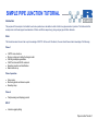
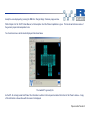
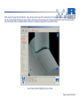
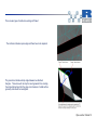
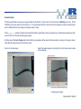
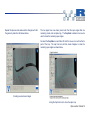
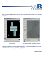
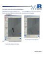
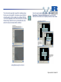
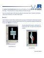
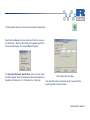
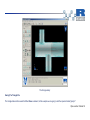
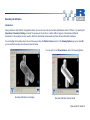
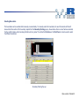
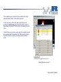
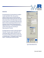
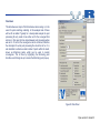
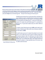
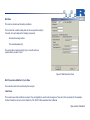
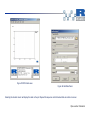
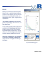
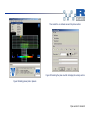
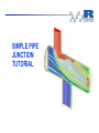
SIMPLE PIPE
JUNCTION
TUTORIAL
SIMPLE PIPE JUNCTION TUTORIAL
Introduction
The purpose of this example is to illustrate how to set-up and solve a calculation in which a fluid in two pipes meets at a junction. The fluid used in this
example is air and the two pipes have diameters of 25mm and 30mm respectively, joining a larger pipe of 40mm diameter.
Aims
This tutorial assumes the user has no prior knowledge of VECTIS. At the end of the tutorial, the user should have a basic knowledge of the following:
Phase 1
·
·
·
·
·
·
VECTIS menu structure.
Moving, scaling and rotating the triangle model.
Stitching incomplete geometries.
CHOP function and MOVE command.
Boundary selection and identification.
Basic mesh set-up.
Phase 5 operation
·
·
·
Solver setup
Monitoring points and reference points.
Boundary setup
Phase 6
·
Postprocessing and displaying results
RPLOT
·
Interactive graph plotting
Pipe Junction Tutorial 1
Pre Processor - Phase 1
Reading-in CAD Geometry
The first stage of performing a CFD analysis with VECTIS is to import the STL 3-dimensional surface geometry of the fluid domain that will be analysed.
The VECTIS pre-processor called Phase1, contains all the necessary tools to view, repair and modify the imported geometry.
To start Phase 1, from the command line, type phase1 at the command prompt for UNIX and LINUX operating systems. For WINDOWS operating
systems start Phase1 from the Start Menu > Programs > Ricardo > Phase1 menu.
As this is the first tutorial we will work from the absolute basics. For a CFD analyst work invariably starts with CAD geometry of some kind. In this case
we will start with an .stl file.
In Phase1 using the File > Open option it is possible to find and select your pipej.stl
file which should have been copied to your working directory.
After selecting the pipej.stl file from the Open File popup window the triangulation merge
tolerance pop up window appears.
For almost all STL files the value shown can be accepted by selecting the OK button on the
pop up window.
The triangulation merge tolerance shown in the pop up window is the shortest
distance between any two triangle nodes in the STL file.
When the tolerance has been accepted and Phase1 loads the STL file any nodes
that have a separation distance shorter than the value shown will be merged
together.
Pipe Junction Tutorial 2
Accept the value displayed by pressing the OK in the Triangle Merge Tolerance popup window.
Within Chapter 2 of the ‘VECTIS User Manual’, a full description of all the Phase1 capabilities is given. This tutorial will introduce some of
the geometry repair and manipulation tools.
You should now have a similar model display as that shown below:
The loaded STL geometry file
As the STL file is being loaded into Phase1 the information is written to the text panel located at the bottom of the Phase1 window. A copy
of this information is shown blow with the reason it is displayed.
Pipe Junction Tutorial 3
The output to the Phase1 text window as the STL file is being loaded.
Pipe Junction Tutorial 4
The key points to note here are that the geometry size limits can be checked to ensure that the loaded geometry is the correct size. A
common error when exporting the STL file from the CAD program is to use the wrong units i.e. inches instead of meters. Also the number
of open edges is reported - these must be closed for the VECTIS automatic mesh generator - the methods used to do this will be outlined
below.
When a geometry file is loaded into Phase1 the Viewing Options panel and the Stitching tools panel are also displayed as shown above.
These panels are used to change the geometry viewing options and repair or modify the the geometry.
After loading the STL file the first action is to save the file in a VECTIS format. VECTIS geometry files are called *.tri files. So using the
File > Save As menu options save the file to pipej.tri in your working directory.
The model can display can be altered using the following techniques:
ZOOM - Press the CTRL button on your keyboard and press and hold the
middle mouse button. Move the mouse to change the view port zoom factor.
CTRL +
Note - if your mouse does not have a middle button then press the left and right
buttons together to perform the same operation
Pipe Junction Tutorial 5
TRANSLATE - Press and hold the middle mouse button and then move the
mouse to translate the viewport position.
Note - if your mouse does not have a middle button then press the left and right
buttons together to perform the same operation
ROTATION - Press the SHIFT button on your keyboard and press and hold the
middle mouse button. Move the mouse to rotate the view port view.
SHIFT +
Note - if your mouse does not have a middle button then press the left and right
buttons together to perform the same operation
Pipe Junction Tutorial 6
ZOOM WINDOW - Press the RIGHT mouse button and dragging a
CENTRE THE VIEW PORT - Press the right mouse button at the
box over the required zoom area.
required centre position and then press the LEFT mouse button.
Pipe Junction Tutorial 7
VIEW RESET - Click on the VIEW RESET BUTTON in the Viewing options window.
Pipe Junction Tutorial 8
When viewing the geometry within phase1, many red lines can be seen at the intersections of the separate surfaces originating from the
STL file, these indicate that there are gaps or holes in the model as shown below. One of the requirements of the VECTIS mesh generator
is that the surface data is completely closed, therefore it is necessary to repair all the areas with red lines.
View of Gaps in Model highlighted by the red lines
Pipe Junction Tutorial 9
There are two types of visible line warnings in Phase1.
The red lines indicate an open edge and these have to be repaired.
The green lines indicate a sharp angle between two attached
triangles. These lines will not stop the mesh generator from creating
the computational mesh but they may occur because of a bad surface
geometry and should be investigated.
Pipe Junction Tutorial 10
Geometry Repair
This can be performed in many ways using commands like the ‘Delete’, ‘Create’ and ‘Join’ tools from the the Stitching icon menu. With in
the Stitching icon menu there is an auto stitch tool - it is recommended that this is only used once the geometry has been visually checked
and it is believed that the open edges are relatively simple to close.
For the pipej.tri geometry that has been loaded into Phase1 we will firstly create two triangles to join the disconnected pipes and then
use the CAP tool to close the remaining open edges.
So firstly select the Create Triangle tool from the stitching icon palette and then select the three nodes by zooming in to the region shown
below and left clicking the mouse on the three nodes.
Zoom in to the area shown
Select the create triangle icon and right click on the three nodes to create
the new triangle.
Creating a new triangle
Pipe Junction Tutorial 11
Repeat this process and create another triangle such that
the geometry looks like that shown below.
The two pipes have now been joined such that the open edges that are
remaining create and complete ring. The Cap Hole command can now be
used to close the remaining open edges.
So select the Cap Hole icon and then left click the mouse on a red line that is
part of the loop. The cap hole tool will then create triangles to close the
remaining open edges as shown below.
Creating a second new triangle
Using the Cap Hole tool to close the open loop
Pipe Junction Tutorial 12
Another part of the model that has open edges is shown below. Firstly zoom into the area and rotate the geometry so that the problem area
is clearly visible.
Next problem area
View zoomed in and rotated to view the problem more clearly.
It can be seen that the triangles in this region have not been connected correctly. This problem is usually caused when the CAD software
is creating the STL file. However it is easy to fix in Phase1 using the repair tools.
Pipe Junction Tutorial 13
Firstly the problem triangles must be deleted using the Delete Triangle icon.
Select the Delete Triangle icon and then left click twice on the
triangles to delete them such that the geometry looks like that shown
Then use the Cap Hole tool to close the open edges such that the
geometry now looks like that shown below.
The repaired region after using the cap hole tool.
below.
The geometry after deleting the problem triangles
Pipe Junction Tutorial 14
The Join function (see right) is useful for combining nodes
that are very close together. It produces a green circle that
should be used to ring the nodes to be combined. With the
‘Join’ button depressed, click for the centre of the circle then
hold and drag to alter its size. Any nodes within the circle
when the mouse is released will be combined.
Once the repair operations have been completed the
Operations > Check for Unstitched option can be used to
make sure the model is now completely closed as shown below.
Joining Nodes using the Join tool
Pipe Junction Tutorial 15
The Operations > Check for Self-Intersections function can be used in the same way. This checks to see if any triangles intersect with
other triangles. This tutorial model should not contain any intersections and it should now be saved.
If any errors are made at this stage, the ‘Undo’ function can usually restore a limited number of actions. It should also be noted that these
functions should be used with care, as it is possible to distort the model.
Moving Face
In order to illustrate some of phase1’s ability to manipulate geometry we are going to extrude the large 40 mm diameter pipe in the positive x
direction to move the downstream boundary further away from the junction itself. This can be performed by marking the right-hand end face
of the pipe using the Mark Area icon as shown below.
After double clicking the left mouse button - rotate the geometry so
that the end face is visible. The triangles on this face should now be
marked red.
Using the Mark Area tool
The marked triangles.
Pipe Junction Tutorial 16
The Move Marked Area Icon is then used to translate the marked face.
Select the Move Marked Area icon and then left click the mouse on
the marked face. When the Move What panel appears select OK to
choose the default option of Connected/Marked Triangles.
The Geometry Movement Specification panel as shown below
should then appear. Enter the parameters as shown below which are
translate by 0.04 meters in the 1,0,0 direction (i.e. X direction).
Move Options Pop up window
Then select OK and the marked face will be moved so that the
geometry should look like that below.
Pipe Junction Tutorial 17
The final geometry
Saving The Triangle File
The triangle data can the saved the File > Save command; in this example we are going to call the repaired model "pipej.tri".
Pipe Junction Tutorial 18
Boundary Identification
Introduction
Having obtained a fully stitched, triangulated surface, the user can now enter the boundary identification section of Phase 1, by selecting the
Operations > Boundary Painting command. The purpose of this section is to define different regions of the surface as different
boundaries. In this example, the user needs to define the boundaries that are walls and those that are inlet/outlet boundaries.
You can display the boundary colours in one of two ways. Using the Outline Colours section of the Viewing Options pop-up set to multi
you can see the boundary colour shown as lines as below
You can also turn on Show Surfaces, also in the Viewing Options.
Boundary Definitions Line display
Boundary Definition Surface Model
Pipe Junction Tutorial 19
Selecting Boundaries
The boundaries can be selected either manually or automatically. To manually select the boundaries, the user first selects with the left
mouse button the number of the boundary required from the Boundary Painting pop-up, shown below. Once a colour has been selected,
the five cells that make up the boundary definition will turn yellow. Then either the Paint Line or the Paint Face tool can be used to select
the different boundaries.
Boundary Painting Pop-up
Pipe Junction Tutorial 20
The boundaries regions required for this example are the 4 pipe
ends which will be inlets or outlets and the pipe wall.
To paint a boundary surface firstly add 4 new boundaries by
pressing the Add Boundary tab and select boundary number 2 in
the Boundary list panel such that the row for the boundary becomes
yellow.
The Mark Face tool can now be used to paint the triangles that need
to be associated with this boundary type. After selecting the Mark
Face tab left click the mouse on the upper pipe face as shown
below.
Painting Boundary number 2
Pipe Junction Tutorial 21
Repeat this process until the boundary setup is as shown on the
right. If necessary triangles can be dragged from one boundary to
another by pressing and holding the left mouse button in the #tri
column of the original boundary and dragging the mouse to the new
boundary column.
Final boundary identification
Pipe Junction Tutorial 22
Boundary Types Definition
Having defined which triangles are associated with each boundary as shown in above each boundary needs to be assigned to one of the
types defined in the table below.
Wall
Zero gradient (symmetry plane)
Inlet/outlet
Cyclic symmetry
This is performed by using the left mouse button in the Type column and selecting the relevant boundary type.
Once the user has completed the selection of the boundaries and assigned the correct types to each, the boundary and types data can be
saved. This is achieved by simply saving the geometry using File > Save or File > Save As to the file pipej.tri.
Mesh Specification
Select the Toolbars > Mesh setup menu. The purpose of this section of Phase 1 is to set up the global control mesh lines which Phase 2
uses as the basis for mesh generation. The mesh setup tools are activated by selecting the Toolbars > Mesh Setup option in the Phase1
menu. This will then display the default outline mesh, which can be manipulated to provide the required control mesh. Alternatively an
existing control mesh can be loaded in using the standard File > Open menu option. A full description of the functionality of the Mesh Menu
is described in Chapter 2 of the VECTIS Documentation/User’s Manual.
For this example, a simple uniformed mesh of 31 x 25 x 11 is used with the default value of 2 used for boundary refinement. From the mesh
setup toolbar the positions of the controlling red lines can be manipulated and the number of divisions as well as the position of local IJK
refinement blocks can be setup. The VECTIS control mesh must always have two red lines which are completely outside all the geometry.
The icons used for the mesh setup are shown by Figure 18.
Pipe Junction Tutorial 23
Figure 18 Control Mesh Tools
Pipe Junction Tutorial 24
Use the mesh tools described above to setup the mesh as shown below with the number of divisions being 31, 25 and 11 in the I,J and K
directions respectively. This will result in the model having approximately 12,500 internal cells. The mesh is shown in Figure 19 .
Figure 19 Control Mesh
Pipe Junction Tutorial 25
The global control mesh has now been set up with out any local refinement blocks. The use of local refinement blocks is determined by the
necessity to provide a greater mesh density in detailed regions of the flow field. These refinement blocks are often referred to as IJK blocks.
As an example of the use of refinement blocks the tutorial will now be add an IJK block over the lower pipe geometry. In order to add or edit
the refinement blocks the IJK Refinement Blocks navigation menu is used. This is shown in Figure 20 .
Figure 20 IJK Block navigation
Pipe Junction Tutorial 26
This panel allows for the addition of IJK blocks by pressing the Add button and then using the mouse to draw a box over the mesh cells
which sets the limits of the IJK block. The left mouse button should continue to be pressed until the box is of the right size. The IJK limits
can then be set in the other co-ordinate plane by changing the view of the mesh and using the Edit button to again draw a box for the
required IJK block limits. The Edit button can also be used to adjust the position of the IJK block once it has been added. Continue the
tutorial by using this IJK block addition procedure to add the refinement block as shown by Figure 21.
Figure 21 IJK block location for tutorial control mesh
Pipe Junction Tutorial 27
The level of refinement applied by this IJK block is determined by the DEEP and FORCE factors which are entered in the IJK navigation pop
up window. The DEEP value determines the refinement applied to the cells at the surface whilst the FORCE value defines the level of
refinement applied to internal cells within the IJK block. The refinement of cells in the IJK block determined by both the DEEP and FORCE
values is defined as each global cell being divided by 2 to the power of the DEEP and FORCE values. That is if the DEEP and FORCE
values are 1 then each global cell is divided by 21 = 2. Likewise if the DEEP and FORCE values were set to 2 then each global cell would be
divided by 22 = 4.
For this tutorial set the refinement value DEEP to 2 and FORCE value to 1. It should be noted that whenever using the IJK refinement
blocks it is important to always maintain a maximum connectivity between cells of 2:1 for accuracy purposes. This can be achieved by using
several IJK blocks with staggered refinement levels.
Mesh Generator - Phase2 and Phase4
Starting Phase 2
To start Phase 2 select Operations > Produce Mesh from the main menu. This will activate the produce mesh menu, as shown in Figure
22. The Mesh input text field requires the name of your mesh file. The output file text field enables you to name your PHASE4 files with the
name of your choice.
Figure 22 Generate Mesh menu for Phase 2
Pipe Junction Tutorial 28
Pressing OK will open a new shell window and start the Phase2 process.
Once the process is complete, two files named PHASE2.DAT and PHASE2.OUT are generated. The Mesh generation process can now
proceed directly to Phase 4, a step that occurs automatically.
Once this process is complete, two files named PHASE4.DAT and PHASE4.OUT are created, unless you have entered your own file name,
in which case PHASE4 will be replaced by your our filename.
The PHASE4.DAT file contains the mesh structure and how it is connected, whilst the PHASE4.OUT file contains the screen output
generated during the Phase 4 process. The PHASE4.DAT and an input file specifying the fluid properties, boundary conditions and
calculation parameters are all that is required to now perform the CFD calculation. The phase2 ‘mesh file name’ and the phase4 commands
can also be typed from the command line.
View Mesh
Meshes can be viewed in phase1 by using the File > Open option as you would any other file
The mesh is viewed as external patches and internal cell faces. The display of cell faces may be toggled on and off by means of the Show
Face option available in the Viewing Options window.
When the View Bounds button is selected (also in the Viewing Options tab), patches are coloured as in the boundary painting menu and
cell faces are coloured grey. When the ‘View Domains’ button is selected, both faces and patches are coloured according to the domain in
which they lie (this only applies to meshes that have been divided into a number of domains, for parallel solution in Phase 5).
You can also view the mesh slice by slice if you wish. By using Operations > Slice Mesh View you can enter limits in the I, J and K
directions allowing you to set how much of the mesh you wish to use. The following keyboard keys can be used to quickly adjust these slice
values.
·
·
DELETE Increases I direction lower and upper limits by 1.
INSERT Decreases I direction lower and upper limits by 1.
Pipe Junction Tutorial 29
·
·
·
·
END Increases J direction lower and upper limits by 1.
HOME Decreases J direction lower and upper limits by 1.
PAGE DOWN Increases K direction lower and upper limits by 1.
PAGE UP Decreases K direction lower and upper limits by 1.
Resetting the View by pressing the VIEW RESET button resets the effect of any previous CHOP operations on the display limits and the
lighting settings.
Figure -23 Viewing the Mesh
SOLVER - Phase 5
Pipe Junction Tutorial 30
Main Input File
This section only covers the applicable topics for this type of calculation - for a full description of all the variables within the input file, please
refer to the appropriate section within the user manual.
The pipej.INP file can be edited using the Phase 5 GUI program. To run Phase 5 GUI from the command prompt type:
phase5gui pipej.INP
This will bring up the first page of the Phase 5 Graphical User Interface Panel.
Pipe Junction Tutorial 31
Iteration Panel
This page allows selection of the timing parameters to be applied to
the model. Select STEADY STATE , then set up the time
parameters as shown in Figure 24. The start time and end time
determine at what iteration number the solution starts at and at what
iteration number it finishes. and the difference between them defines
the number of iterations. Time steps between Postprocessing simply
defines the number of post-processing writes there are in the run. In
steady state runs there is little need to write post-processing files
except at the end of the run. For this tutorial this should be set to 10
so that the solutions progress can be viewed during the
Postprocessing section of the tutorial.
This phase5gui window also controls the overall solution strategy for
the calculation. The pressure-velocity Coupling algorithm can be
selected between SIMPLE and PISO by means of the option menu.
This should be set to SIMPLE since the time base has been selected
as a Steady State analysis. The PISO algorithm is used for transient
analyses. The remaining options should be left as default.
Figure 24 Iteration Selection Panel
Pipe Junction Tutorial 32
Files Panel
This tab allows user input of the file behaviour when saving or, in the
event of system crashing, restarting. In this example most of these
will be left as default. Typically for a steady state analysis the post
processing file only needs to be written out for the converged final
solution. In this case the time steps between post processing writes
was set to 10 so that the convergence can be monitored, therefore
the checkpoint for write post processing file should be left on. It is
also desirable to allocate a small number of points within the mesh,
known as Monitoring points, which can be used to monitor
convergence. This is done by highlighting the Monitoring point
checkbox, and clicking set-up to access the Monitoring point pop-up.
Figure 25 Files Panel
Pipe Junction Tutorial 33
Monitoring locations should be chosen at points of interest in the flow domain and for steady flows should be positioned at points where they
can act as a good indicator of overall convergence. At least one monitoring point must be specified. The positions of the monitoring points
are setup based on either IJK location or XYZ location. IJK co-ordinates are obtained from the control mesh. To setup up the monitoring
points press the Setup button next to the Monitoring point text. The setup for the first monitoring point is shown by Figure 26.
The Monitoring point panel allows the user to specify points within the model domain where
values of the solution are output to a named file at the end of each time step. The specified
filename has the project name and run number added to it, as for all files written by Phase
5. In this example there are three Monitoring points – one at the inlet of the 40mm pipe (I J
K location 6 15 7), another at the outlet of the 40mm pipe (27 15 7), and the third in the
30mm pipe (16 9 7). They must each be allocated a name, such as INLET, OUTLET and
JUNCTION.
To increase the number of Monitoring points, simply click ADD. Select the method by which
the location of the Monitoring point is defined, alter the name of the filename and define the
point. When finished, click DONE.
Figure 26 Monitoring Point Setup window
The restart file options are also set in File window. When restarting from zero the restart
position is set to none whilst there are also other options for restarting an analysis which
has purposely been stopped or crashed. The restart frequency is the number of time steps
between each restart file write. This is a compromise between ensuring that if the
calculation stops it can be restarted without losing to much analysis time whilst also
ensuring that the calculation is not slowed significantly because of the time taken to write
the restart file due disk access issues.
Pipe Junction Tutorial 34
Models Panel
This panel is shown by Figure 27 and it contains all the modelling
parameters for the fluid flow. In here it is possible to specify what the
fluid is, and how it behaves. In this example, only two of the options
are relevant: Species data, the fluid specific heat and viscosity
coefficients at various temperatures. Turbulence, the turbulence
model to be used. Within the Species data set-up box, four fluids are
available for selection and these are Fuel (default is methane), Air,
Products (default is the products of methane and air combustion)
and Inerts (default is nitrogen) – air is the second of these four, and
is the one to be used in this example. The Turbulence set-up box
should be highlighted by default and set to K-Epsilon for this
example.
Figure 27 Models Panel
Pipe Junction Tutorial 35
Solving Panel
This panel is shown by Figure 28 and it contains two sections of interest for this
tutorial; the equations selector and the reference position selector.
The equation selector panel contains, by default, most of the necessary equations to
be solved. Highlighting the passive scalar check box will have the effect of introducing
an electronic "dye" into the flow, which makes the post-processing easier to visualise.
By outputting results frequently, we can watch the passive scalar progress through
the solution as it converges. In this example, the "Start Time" is set to 0 and the "End
Time" is set to 350. This, together with post-processing results written every 10
iterations gives 35 steps with which the "dye" can be seen flowing through the pipe.
For a steady state calculation, it is the final result when a steady solution has been
achieved that is of interest.
The "Reference position" panel allows the user to enter the I, J, K values (determined
by the global mesh) for the reference location. During solution of the pressure
equation, the variable that is monitored is the pressure relative to this reference
location. The position of this location is not critical but is usually chosen to be near the
outlet.
Pressures reporting in the output and monitoring files are relative pressures; the
absolute pressure is the sum of the relative pressure and reference pressure.
In this example, an I, J, K value of 31, 15, 7, would place the reference point close to
outlet boundary number 4.
Figure 28 Solving Panel
Pipe Junction Tutorial 36
Boundary Panel
The boundary tab is the area where the majority of the input
information is delivered. It defines the flow directions and profiles for
inlet/outlet boundaries, and defines the properties of the wall
boundaries. Note that the flow rates, composition and
thermodynamic quantities are defined in the Zero-dimensional data
panel.
Figure 29 Boundary Panel
Pipe Junction Tutorial 37
Inlet/Outlet
There should be an Inlet/Outlet Boundary module for every inlet/outlet
boundary in the mesh. The following must be specified in each module:
Universal boundary number is the number of the universal boundary to which
the data set applies. Refer to the plot in Phase 1 Figure 16 Boundary
Definition Surface Model.
Zero-dimensional data set number is the zero-dimensional data set number
with which the boundary is associated – see Zero-Dimensional Data, below.
The inlet profile information is not used for a boundary that is exclusively an
outlet. Conversely, the outlet profile option is not used for exclusively inlet
boundaries. However, both sets of information are included for all inlet/outlet
boundaries, since the zero-dimensional data set determines whether the
boundary is an inflow or an outflow at any given time in the calculation.
Figure 30 Inlet/Outlet Pop-up Panel
Inlet specification defines the velocity profile at the inlet boundary. The types available are:
·
·
·
Uniform profile with a given direction defined by the user.
Radial variation about a given axis.
Default normal profile where the program sets the velocity profile to be uniform and normal to the inlet.
Outlet allows the user to specify the type of outlet velocity profile. By selecting Mirrored, the outlet profile is determined by the profile
upstream of the boundary. Selecting Uniform, forces a uniform profile for the normal velocity across the boundary. Uniform is the preferred
option.
Pipe Junction Tutorial 38
Zero-Dimensional Data
This section specifies the mass flow rates, compositions and thermodynamic
quantities for inlet and outlet boundary conditions.
There should be a zero-dimensional data set module for every boundary
referenced in the Inlet/Outlet boundary specification.
For each module, the following must be specified:
Data set number. Specific data set numbers are referenced by inlet/outlet
boundary modules, so having the data set number explicitly included here
removes the need to have zero-dimensional data sets ordered consecutively.
Number of time specifications is the number of times at which data will
be provided.
Flow rate specification allows the user to select the type of flow required.
Prescribed mass flow: specified mass flows are forced at the
boundary.
Pressure boundary: specified pressure field is forced at the boundary.
Figure 31 Zero-Dimensional Data Set Pop-up
Pipe Junction Tutorial 39
The Setup Flow Parameters button brings up a panel that allows the user to define the bounadray data values for each time specification.
These are:
·
·
·
·
·
·
·
·
·
·
·
·
Non-dimensional time.
Mass flow rate (kg/s). Ignored if pressure boundaries are used. A
positive value indicates inflow; a negative value indicates outflow.
Effective flow area (m2), (Always ignored for currently available
boundary types).
Temperature (K).
Pressure (Pa).
Turbulence intensity as fraction of inlet velocity.
Turbulence length scale (m).
Passive scalar.
Fuel mass fraction.
Oxidant mass fraction.
Products mass fraction.
Inert mass fraction.
Figure 32 Zero-dimensional Flow Parameters Panel
Pipe Junction Tutorial 40
In this example, Zero Dimensional Boundaries 1, 2, 3 and 4 are defined as inlet/outlet boundaries and the respective boundary conditions
are given in Table 2; the fluid used is air.
Boundary
Number
Description
Boundary Condition
1
Left Hand Inlet (40mm)
Mass Flow = +0.0135 kg/s
2
Upper Inlet (25mm)
Mass Flow = +0.0105 kg/s
3
Bottom Outlet (30mm)
Static Pressure Boundary = 100000 Pa
4
Right Hand Outlet (40mm)
Static Pressure Boundary = 100000 Pa
Table 2 Inlet/Outlet Boundary Specification
Pipe Junction Tutorial 41
Wall Data
This section contains wall boundary conditions.
There should be a wall boundary data set for every wall boundary in
the mesh. For each data set the following is required:
Universal boundary number.
The wall temperature (K).
The wall surface roughness height (m). A smooth surface is
represented by a value of zero.
Figure 33 Wall Boundary Panel
Wall Temperature Modifier & Cyclic Data
These sections will not be used during this example.
Initial Panel
This is where any initial conditions are input. They will typically be used to aid convergence. They will not be necessary for this example.
Further information can be found in Chapter 6 of the VECTIS Documentation/User’s Manual.
Pipe Junction Tutorial 42
Solver
Once the input file is complete, this can be submitted to the CFD solver typing the following at the command line.
phase5 pipej.INP
Solver output information during run time
As phase5 is performing the iterations required to generate the final converged solution it prints some vital information to the window from
which it was launched. Figure 34 below shows an example of this output. It includes the equation residuals for each equation being solved
which can be used to monitor the solutions progress towards the converged solution. It should be noted that usual convergence criteria
dictates that the residuals are below a defined value such as 10-4 or 10-6. For the momentum, temperature and Turbulence Residuals this
can apply however the definition of the pressure residual relies on a time dependant variable. Therefore for steady state analyses the
pressure residual can be used to monitor for convergence based on its magnitude of change from one time step to another. If this change is
small then it can be deemed that the computation has converged.
The average values from the monitoring points for each variable are also printed to the screen.
The velocity correction information is also printed to the screen - this is a useful indication as to the stability of the solution. The correction
values should typically be an order of magnitude smaller than the actual velocity values i.e. 10 times smaller. The maximum cell Reynolds
number is also printed to the screen and the reference pressure. This tutorial is a steady state analysis and so consequently none of the
CFD solver parameters that are generated during transient analyses are present. These will be discussed in tutorial 3 and the information
for these output parameters can also be found in the VECTIS user manual.
Pipe Junction Tutorial 43
Figure 34 Solver output during run time
The calculation is set to run for 350 iterations. The solution can be monitored and the results can be plotted using Ricardo’s RPLOT
program and the VECTIS Post Processor Phase6, the use of which is outlined in section 1.8 below.
Pipe Junction Tutorial 44
RPLOT
Overview
RPLOT is an interactive plotting package developed by Ricardo to display graphical output from its engineering analysis software tools. The
purpose of this tutorial is to outline the basic features of RPLOT , in order to allow users to produce plots of data generated during the
Basic Operation
Reading Data
Typically the first task when running RPlot is to add axes. For the data produced in this example, a simple X-Y plot is the most suitable. To
perform this, click on the Add > Plot > XY option in the taskbar. The screen should then show a blank set of axes, as in Figure 35.
Data can now be displayed. To do so, click on the Add > Data option in the taskbar, then click on the graph area. A panel will be displayed
from which data can be read in. This is shown in Figure 36.
The raw data to be plotted is stored in the Monitoring files saved during the Phase 5 solver stage. To access these, click on the file icon in
the top right of the Add Data panel. This will bring up a browser where it is possible to load the file. The following instructions guide the user
through the first plot – further plots can be added as desired.
The first plot to be drawn is the relative values, i.e. the values relative to the reference position. This is a good gauge of convergence.
Selecting pipe.JUNCTION_001 will bring up a further Add ASCII Data Panel popup that requires selection of column lists. The monitoring
files are tables (visible using the "more filename" command at the command line or a text editor) of data recorded at each iteration during
Phase 5. You can see what is contained in each column of each output file at the top of the pipej.OUT_001 file.
Pipe Junction Tutorial 45
Figure 35 RPlot blank axes
Figure 36 Add Data Panel
Selecting the desired column will display the data on the plot. Repeat this sequence until all desired data are visible on screen.
Pipe Junction Tutorial 46
Editing Plots
Most editing of axes, labels and titles can be performed by doubleclicking on the item to be altered. One improvement in clarity to be
considered on this plot is changing the Y-axis to a log scale. Doubleclick on the Y-axis – it should turn red after the first click – and a
panel will appear with a number of options. Change the TYPE box to
"Log" and click Enter.
To alter the legend of the line, double-click on the current legend
(probably currently labelled "pipej"). In the miscellaneous box, under
legend, change as desired.
Two types of heading exist, labelled "Heading" and "Title". These are
accessed by clicking on the Add > Heading or Add > Title tabs in
the taskbar. A prompt to pick the plot to which the title/heading
should be added to appears in the lower prompt box – click on one
of the lines on the current plot. Headings are located centrally at the
top of the plot, and titles are positioned at the top of the Y-axis.
A date is visible to the top right of the plot. To alter this, double-click
on it. Options exist for adding gridlines, plot identification codes,
altering the date or time, and changing the location of the legend.
Alter as required.
Figure 37 Data Plot Showing Log Scale
Pipe Junction Tutorial 47
Post-processing – Phase 6
Once the calculation is complete, the results can be viewed using the phase6 GUI postprocessor.
Phase6 can be started from a command line (UNIX and Linux platforms) or from the Programs Start Menu for Windows NT/2000 platforms.
To start Phase 6 from the command line, type:
phase6 pipej.POST_001
Once the post-processing file has been loaded, all the commands can be executed using either the menu or the command line.
Figure 38 and 39 below show how to add a velocity plane.
Pipe Junction Tutorial 48
Then select the co-ordinate axis and the plane number.
Figure 39 Selecting the plane in which to display the velocity vectors
Figure 38 Adding planar plots in phase6
Pipe Junction Tutorial 49
Figure 38 shows a velocity field centrally through the model.
The plot can also be added using the command line in phase6. This is the approach used if the user wishes to use a batch file to
generate many different plots. The commands for this example are:
PLOT ADD MESHGEOMETRY k7
PLOT ADD VELOCITY CELL k7
K7 is selected to give a cut-through down the middle of the 11 cells in the K direction.
Other plots such as the mesh cell outline as in Figure 38 or scalar planar plots such as the relative pressure can also be added by selecting
the appropriate menu.
During the calculation, results are written to the post-processing file every 10 iterations. Therefore, the plot shown in Figure 38 is the first set
of results in the file. The results for other iteration positions can be shown by animating the results through the Time Control > Animate
menu or using the Time Control > Position option.
Surface variables can also be plotted using the Plot > Add > Patch Scalar option as shown by figure 40 below. A popup window giving
the user the choice of solid or Gouraud shading is then shown. Solid shading plots a surface profile using all the near wall cell centre values
whilst Gouraud shading plots the variable values using all the cell corner nodes which creates a smoother profiled plot.
Pipe Junction Tutorial
Choose Gouraud shading.
Figure 40 Adding a Gouraud Surface Plot
Pipe Junction Tutorial 51
The choice of variable to be displayed on the surface plot is made through the Plot > Scalars menu.
Choose Relative Pressure to generate a similar plot to that shown in figure 41 below.
Pipe Junction Tutorial 52
Figure 41 Surface Relative Pressure
The minimum and maximum scale for the variables being displayed can be adjusted by using the Options > Scales pop up window as
shown by Figure 42 below.
Figure 42 Scale range adjustment pop up window.
This ends the pipe junction tutorial
Pipe Junction Tutorial 53