1
Extended SCEPTRE
Volume 1
User’s Manual
David Becker
GTE Sylvania, Incorporated
Revised and edited by
Wolf-Rainer Novender
D-64625 Bensheim - Germany
Oktober 1999
Contents
1. Introduction
1
1.1. SCEPTRE capabilities . . . . . . . . . . . . . . . . . . . . . . . . . . . . . . . . . . . . . . . .
1
1.2. Handbook coverage . . . . . . . . . . . . . . . . . . . . . . . . . . . . . . . . . . . . . . . . . .
2
1.3. Input data example . . . . . . . . . . . . . . . . . . . . . . . . . . . . . . . . . . . . . . . . . .
2
2. SCEPTRE use
4
2.1. Circuit preparation . . . . . . . . . . . . . . . . . . . . . . . . . . . . . . . . . . . . . . . . . .
4
2.2. Preparing the SCEPTRE input data . . . . . . . . . . . . . . . . . . . . . . . . . . . . . . . . . .
5
2.2.1. Headings and subheadings . . . . . . . . . . . . . . . . . . . . . . . . . . . . . . . . . .
5
2.2.2. Elements . . . . . . . . . . . . . . . . . . . . . . . . . . . . . . . . . . . . . . . . . . .
8
2.2.3. Defined parameters . . . . . . . . . . . . . . . . . . . . . . . . . . . . . . . . . . . . . .
15
2.2.4. Outputs . . . . . . . . . . . . . . . . . . . . . . . . . . . . . . . . . . . . . . . . . . . .
17
2.2.5. Initial Conditions . . . . . . . . . . . . . . . . . . . . . . . . . . . . . . . . . . . . . . .
20
2.2.6. Functions . . . . . . . . . . . . . . . . . . . . . . . . . . . . . . . . . . . . . . . . . . .
22
2.2.7. Run controls . . . . . . . . . . . . . . . . . . . . . . . . . . . . . . . . . . . . . . . . .
26
2.2.8. DC options . . . . . . . . . . . . . . . . . . . . . . . . . . . . . . . . . . . . . . . . . .
38
2.2.9. Program limits . . . . . . . . . . . . . . . . . . . . . . . . . . . . . . . . . . . . . . . .
40
2.2.10. Vectorized notation . . . . . . . . . . . . . . . . . . . . . . . . . . . . . . . . . . . . . .
41
2.2.11. Internal Parameters . . . . . . . . . . . . . . . . . . . . . . . . . . . . . . . . . . . . . .
41
2.3. Stored model feature . . . . . . . . . . . . . . . . . . . . . . . . . . . . . . . . . . . . . . . . .
44
2.3.1. Transistor model insertion . . . . . . . . . . . . . . . . . . . . . . . . . . . . . . . . . .
44
2.3.2. N terminal model storage . . . . . . . . . . . . . . . . . . . . . . . . . . . . . . . . . . .
46
2.3.3. Changes to a stored model . . . . . . . . . . . . . . . . . . . . . . . . . . . . . . . . . .
47
2.3.4. Initial conditions for a stored model . . . . . . . . . . . . . . . . . . . . . . . . . . . . .
49
2.3.5. Model deletion . . . . . . . . . . . . . . . . . . . . . . . . . . . . . . . . . . . . . . . .
49
2.4. RERUN feature . . . . . . . . . . . . . . . . . . . . . . . . . . . . . . . . . . . . . . . . . . . .
49
2.4.1. General usage . . . . . . . . . . . . . . . . . . . . . . . . . . . . . . . . . . . . . . . . .
49
2.4.2. Limitations of the rerun feature . . . . . . . . . . . . . . . . . . . . . . . . . . . . . . .
51
i
2.5. CONTINUE feature . . . . . . . . . . . . . . . . . . . . . . . . . . . . . . . . . . . . . . . . . .
54
2.5.1. General usage . . . . . . . . . . . . . . . . . . . . . . . . . . . . . . . . . . . . . . . . .
54
2.5.2. Limitations on the CONTINUE feature . . . . . . . . . . . . . . . . . . . . . . . . . . .
55
2.6. RE-OUTPUT feature . . . . . . . . . . . . . . . . . . . . . . . . . . . . . . . . . . . . . . . . .
55
2.7. Subprogram capability . . . . . . . . . . . . . . . . . . . . . . . . . . . . . . . . . . . . . . . .
56
2.7.1. Subprogram insertion . . . . . . . . . . . . . . . . . . . . . . . . . . . . . . . . . . . . .
58
2.7.2. Subprogram with models . . . . . . . . . . . . . . . . . . . . . . . . . . . . . . . . . . .
58
2.8. Additional output and control . . . . . . . . . . . . . . . . . . . . . . . . . . . . . . . . . . . . .
58
2.8.1. SIMUL8 program data . . . . . . . . . . . . . . . . . . . . . . . . . . . . . . . . . . . .
59
2.8.2. No element sort . . . . . . . . . . . . . . . . . . . . . . . . . . . . . . . . . . . . . . . .
59
2.8.3. Matrix printouts . . . . . . . . . . . . . . . . . . . . . . . . . . . . . . . . . . . . . . .
59
2.8.4. Nodal listing . . . . . . . . . . . . . . . . . . . . . . . . . . . . . . . . . . . . . . . . .
59
2.8.5. AC matrix outputs . . . . . . . . . . . . . . . . . . . . . . . . . . . . . . . . . . . . . .
60
2.8.6. Program Debug Output . . . . . . . . . . . . . . . . . . . . . . . . . . . . . . . . . . . .
60
2.9. Error diagnostics . . . . . . . . . . . . . . . . . . . . . . . . . . . . . . . . . . . . . . . . . . .
60
3. Equivalent circuits and associated notation
66
3.1. Diodes . . . . . . . . . . . . . . . . . . . . . . . . . . . . . . . . . . . . . . . . . . . . . . . . .
66
3.2. Transistors (large signal equivalent) . . . . . . . . . . . . . . . . . . . . . . . . . . . . . . . . .
67
3.3. Transistors (small signal equivalent) . . . . . . . . . . . . . . . . . . . . . . . . . . . . . . . . .
73
3.4. Insertion of basic radiation effects . . . . . . . . . . . . . . . . . . . . . . . . . . . . . . . . . .
75
4. Examples of SCEPTRE Use
79
4.1. Example 1 - INVERTER CIRCUIT LOADED WITH RC NETWORK (A01) . . . . . . . . . . .
79
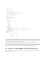
4.2. Example 2 - TRANSFORMER COUPLED AMPLIFIER (A02) . . . . . . . . . . . . . . . . . .
80
4.3. Example 3 - DARLINGTON PAIR (A03) . . . . . . . . . . . . . . . . . . . . . . . . . . . . . .
83
4.4. Example 4 - USE OF SMALL SIGNAL EQUIVALENT CIRCUIT (A04) . . . . . . . . . . . . .
86
4.5. Example 5 - SOLUTION OF SIMULTANEOUS DIFFERENTIAL EQUATIONS (A05) . . . . .
87
4.6. Convolution example . . . . . . . . . . . . . . . . . . . . . . . . . . . . . . . . . . . . . . . . .
89
4.6.1. General . . . . . . . . . . . . . . . . . . . . . . . . . . . . . . . . . . . . . . . . . . . .
89
4.6.2. Convolution impedance mode . . . . . . . . . . . . . . . . . . . . . . . . . . . . . . . .
89
4.6.3. Convolution admittance mode . . . . . . . . . . . . . . . . . . . . . . . . . . . . . . . .
90
4.6.4. Sample problem . . . . . . . . . . . . . . . . . . . . . . . . . . . . . . . . . . . . . . .
91
4.7. Example 7 - USE OF MONTE CARLO (A07) . . . . . . . . . . . . . . . . . . . . . . . . . . . .
94
4.8. Example 8 - USE OF SENSITIVITY (A08) . . . . . . . . . . . . . . . . . . . . . . . . . . . . .
95
4.9. Example 9 - USE OF WORST-CASE (A09) . . . . . . . . . . . . . . . . . . . . . . . . . . . . .
99
4.10. Example 10 - USE OF OPTIMIZATION (A10) . . . . . . . . . . . . . . . . . . . . . . . . . . . 100
4.11. Example 11 - USE OF AC ANALYSIS (A11) . . . . . . . . . . . . . . . . . . . . . . . . . . . . 103
4.12. Example 12 - TRANSFER FUNCTION SIMULATION . . . . . . . . . . . . . . . . . . . . . . . 105
ii
A. Appendices
109
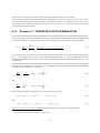
A.1. Topological restrictions on SCEPTRE . . . . . . . . . . . . . . . . . . . . . . . . . . . . . . . . 109
A.1.1. Restrictions on AC, transient and initial condition solutions . . . . . . . . . . . . . . . . . 109
A.1.2. Restrictions on initial condition solutions . . . . . . . . . . . . . . . . . . . . . . . . . . 109
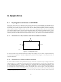
A.2. Computational delay . . . . . . . . . . . . . . . . . . . . . . . . . . . . . . . . . . . . . . . . . 110
A.3. Special options in initial conditions computation . . . . . . . . . . . . . . . . . . . . . . . . . . . 110
A.3.1. Initial conditions computation via transient analysis . . . . . . . . . . . . . . . . . . . . . 111
A.3.2. Reruns with the DC algorithm . . . . . . . . . . . . . . . . . . . . . . . . . . . . . . . . 112
A.3.3. Optional initial conditions for transient reruns . . . . . . . . . . . . . . . . . . . . . . . . 114
A.4. Specified print interval . . . . . . . . . . . . . . . . . . . . . . . . . . . . . . . . . . . . . . . . 114
A.5. Composite plots . . . . . . . . . . . . . . . . . . . . . . . . . . . . . . . . . . . . . . . . . . . . 115
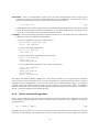
A.6. Nodal listings . . . . . . . . . . . . . . . . . . . . . . . . . . . . . . . . . . . . . . . . . . . . . 117
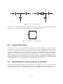
A.7. Differential equation identification . . . . . . . . . . . . . . . . . . . . . . . . . . . . . . . . . . 117
A.8. Convolution analysis . . . . . . . . . . . . . . . . . . . . . . . . . . . . . . . . . . . . . . . . . 119
A.8.1. Introduction . . . . . . . . . . . . . . . . . . . . . . . . . . . . . . . . . . . . . . . . . . 119
A.8.2. Mixed-domain approach . . . . . . . . . . . . . . . . . . . . . . . . . . . . . . . . . . . 120
A.8.3. Network situations for which the convolution analysis may apply . . . . . . . . . . . . . 121
A.8.4. Integration routine . . . . . . . . . . . . . . . . . . . . . . . . . . . . . . . . . . . . . . 121
A.8.5. Impedance model . . . . . . . . . . . . . . . . . . . . . . . . . . . . . . . . . . . . . . . 123
A.8.6. Admittance model . . . . . . . . . . . . . . . . . . . . . . . . . . . . . . . . . . . . . . 124
A.8.7. Storing impulse response functions . . . . . . . . . . . . . . . . . . . . . . . . . . . . . 125
A.9. Notes to the SCEPTRE User . . . . . . . . . . . . . . . . . . . . . . . . . . . . . . . . . . . . . 126
A.9.1. Specification of dependent sources . . . . . . . . . . . . . . . . . . . . . . . . . . . . . . 126
A.9.2. Proper use of dependent sources . . . . . . . . . . . . . . . . . . . . . . . . . . . . . . . 127
A.9.3. Avoiding computational delay . . . . . . . . . . . . . . . . . . . . . . . . . . . . . . . . 128
A.9.4. Overcoming restrictions in initial conditions runs . . . . . . . . . . . . . . . . . . . . . . 128
A.9.5. Error checking in IC VIA IMPLICIT . . . . . . . . . . . . . . . . . . . . . . . . . . . . 128
A.9.6. Element sort . . . . . . . . . . . . . . . . . . . . . . . . . . . . . . . . . . . . . . . . . 129
A.9.7. Output reduction . . . . . . . . . . . . . . . . . . . . . . . . . . . . . . . . . . . . . . . 129
A.9.8. Some frequent errors . . . . . . . . . . . . . . . . . . . . . . . . . . . . . . . . . . . . . 129
A.9.9. DC coupling capacitor in certain AC runs . . . . . . . . . . . . . . . . . . . . . . . . . . 129
A.9.10. Convolution input . . . . . . . . . . . . . . . . . . . . . . . . . . . . . . . . . . . . . . . 129
A.9.11. Voltmeters and Ammeters . . . . . . . . . . . . . . . . . . . . . . . . . . . . . . . . . . 130
A.9.12. Avoiding redundant sensitivity runs . . . . . . . . . . . . . . . . . . . . . . . . . . . . . 130
A.9.13. Ideal transformers . . . . . . . . . . . . . . . . . . . . . . . . . . . . . . . . . . . . . . 130
A.9.14. Semiconductor capacitance . . . . . . . . . . . . . . . . . . . . . . . . . . . . . . . . . . 130
A.9.15. Rerun . . . . . . . . . . . . . . . . . . . . . . . . . . . . . . . . . . . . . . . . . . . . . 131
iii
List of Figures
1.1. Sample Circuit . . . . . . . . . . . . . . . . . . . . . . . . . . . . . . . . . . . . . . . . . . . .
2
1.2. SCEPTRE Version . . . . . . . . . . . . . . . . . . . . . . . . . . . . . . . . . . . . . . . . . .
3
2.1. Circuit in SCEPTRE Form . . . . . . . . . . . . . . . . . . . . . . . . . . . . . . . . . . . . . .
5
2.2. Mutual Inductance Polarities . . . . . . . . . . . . . . . . . . . . . . . . . . . . . . . . . . . . .
12
2.3. Configurations That Require Source Derivatives . . . . . . . . . . . . . . . . . . . . . . . . . . .
13
2.4. Voltage Polarity and Current Direction . . . . . . . . . . . . . . . . . . . . . . . . . . . . . . . .
21
2.5. TABLE ERIN Values as a Function of Time . . . . . . . . . . . . . . . . . . . . . . . . . . . . .
25
2.6. Example of the Stored Model Feature of SCEPTRE . . . . . . . . . . . . . . . . . . . . . . . . .
45
2.7. Pulse Train . . . . . . . . . . . . . . . . . . . . . . . . . . . . . . . . . . . . . . . . . . . . . .
57
3.1. General Diode Model . . . . . . . . . . . . . . . . . . . . . . . . . . . . . . . . . . . . . . . . .
66
3.2. SCEPTRE Diode Representation . . . . . . . . . . . . . . . . . . . . . . . . . . . . . . . . . . .
67
3.3. Alternate SCEPTRE Diode Representation . . . . . . . . . . . . . . . . . . . . . . . . . . . . . .
67
3.4. Basic Ebers-Moll Transistor Equivalent Circuits . . . . . . . . . . . . . . . . . . . . . . . . . . .
69
3.5. SCEPTRE Ebers-Moll Representations . . . . . . . . . . . . . . . . . . . . . . . . . . . . . . .
71
3.6. Alternate Ebers-Moll Representation . . . . . . . . . . . . . . . . . . . . . . . . . . . . . . . . .
73
3.7. Low Frequency H Parameter Model . . . . . . . . . . . . . . . . . . . . . . . . . . . . . . . . .
74
3.8. SCEPTRE Representation of H Parameter Model . . . . . . . . . . . . . . . . . . . . . . . . . .
74
3.9. Voltage Dependent Primary Photo current . . . . . . . . . . . . . . . . . . . . . . . . . . . . . .
75
3.10. Capacitor Radiation Equivalent Circuit . . . . . . . . . . . . . . . . . . . . . . . . . . . . . . . .
77
4.1. Example 1 Schematic Diagram, SCEPTRE form . . . . . . . . . . . . . . . . . . . . . . . . . . .
79
4.2. Example 1 outputs . . . . . . . . . . . . . . . . . . . . . . . . . . . . . . . . . . . . . . . . . .
81
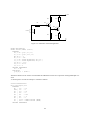
4.3. Schematic of the transformer coupled amplifier, transistor model . . . . . . . . . . . . . . . . . .
82
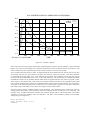
4.4. Example 2 outputs . . . . . . . . . . . . . . . . . . . . . . . . . . . . . . . . . . . . . . . . . .
83
4.5. Schematic of the Darlington Pair . . . . . . . . . . . . . . . . . . . . . . . . . . . . . . . . . . .
84
4.6. Example 3 Output Listings . . . . . . . . . . . . . . . . . . . . . . . . . . . . . . . . . . . . . .
85
4.7. Schematic of Example 4, Low Frequency h Parameter Equivalent Circuit . . . . . . . . . . . . . .
86
iv
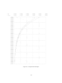
4.8. Plot of VRL1 versus TIME . . . . . . . . . . . . . . . . . . . . . . . . . . . . . . . . . . . . . .
87
4.9. Plot of VRL2 versus TIME . . . . . . . . . . . . . . . . . . . . . . . . . . . . . . . . . . . . . .
88
4.10. Convolution Mode Interface . . . . . . . . . . . . . . . . . . . . . . . . . . . . . . . . . . . . .
90
4.11. Convolution Representation Using Series Impedance Elements . . . . . . . . . . . . . . . . . . .
90
4.12. Convolution Representation Using Parallel Admittance Elements . . . . . . . . . . . . . . . . . .
91
4.13. Convolution Sample Problem Reference Schematic . . . . . . . . . . . . . . . . . . . . . . . . .
92
4.14. Convolution Reference Example Output . . . . . . . . . . . . . . . . . . . . . . . . . . . . . . .
93
4.15. Convolution Example, Impedance Model Schematic . . . . . . . . . . . . . . . . . . . . . . . . .
93
4.16. Convolution Sample Problem Output . . . . . . . . . . . . . . . . . . . . . . . . . . . . . . . . .
94
4.17. Monte Carlo Example Outputs . . . . . . . . . . . . . . . . . . . . . . . . . . . . . . . . . . . .
96
4.18. Sensitivity Example Output . . . . . . . . . . . . . . . . . . . . . . . . . . . . . . . . . . . . . .
98
4.19. Worst Case Example Outputs . . . . . . . . . . . . . . . . . . . . . . . . . . . . . . . . . . . . . 100
4.20. Optimization Example Outputs . . . . . . . . . . . . . . . . . . . . . . . . . . . . . . . . . . . . 102
4.21. Schematic - AC Example, Equivalent Circuit . . . . . . . . . . . . . . . . . . . . . . . . . . . . 103
4.22. A Transfer Function Block and the Equivalent SCEPTRE Representation . . . . . . . . . . . . . 107
A.1. Voltage Source Loop . . . . . . . . . . . . . . . . . . . . . . . . . . . . . . . . . . . . . . . . . 109
A.2. Current Source Cut Sets . . . . . . . . . . . . . . . . . . . . . . . . . . . . . . . . . . . . . . . . 110
A.3. Voltage Source - Inductor Loop . . . . . . . . . . . . . . . . . . . . . . . . . . . . . . . . . . . . 110
A.4. Current Source - Capacitor Cut Sets . . . . . . . . . . . . . . . . . . . . . . . . . . . . . . . . . 111
A.5. Composite Plot Example . . . . . . . . . . . . . . . . . . . . . . . . . . . . . . . . . . . . . . . 116
A.6. Circuit to Illustrate a Nodal Listing . . . . . . . . . . . . . . . . . . . . . . . . . . . . . . . . . . 117
A.7. Nodal Listing requested by LIST NODE MAP . . . . . . . . . . . . . . . . . . . . . . . . . . . 118
A.8. Network to Illustrate Differential Equation Identification . . . . . . . . . . . . . . . . . . . . . . 119
A.9. Separation of Linear and Non-Linear Sub-Networks . . . . . . . . . . . . . . . . . . . . . . . . . 121
A.10.Impedance Model . . . . . . . . . . . . . . . . . . . . . . . . . . . . . . . . . . . . . . . . . . . 124
A.11.Admittance Model . . . . . . . . . . . . . . . . . . . . . . . . . . . . . . . . . . . . . . . . . . 125
A.12.Ammeter - voltmeter elements . . . . . . . . . . . . . . . . . . . . . . . . . . . . . . . . . . . . 130
A.13.Ideal Transformer . . . . . . . . . . . . . . . . . . . . . . . . . . . . . . . . . . . . . . . . . . . 130
v
List of Tables
2.1. Units for High-Speed Transistorized Circuits . . . . . . . . . . . . . . . . . . . . . . . . . . . .
5
2.2. Entries under ELEMENTS . . . . . . . . . . . . . . . . . . . . . . . . . . . . . . . . . . . . . .
9
2.3. Functions of Real and Complex Arguments . . . . . . . . . . . . . . . . . . . . . . . . . . . . .
24
2.4. Default run control quantities in SCEPTRE . . . . . . . . . . . . . . . . . . . . . . . . . . . . .
27
2.5. Run controls for specifying mode of analysis . . . . . . . . . . . . . . . . . . . . . . . . . . . .
30
2.6. Additional run controls . . . . . . . . . . . . . . . . . . . . . . . . . . . . . . . . . . . . . . . .
39
2.7. Dependent variables in DC calculations. . . . . . . . . . . . . . . . . . . . . . . . . . . . . . . .
40
2.8. Independent variables in DC calculations. . . . . . . . . . . . . . . . . . . . . . . . . . . . . . .
40
2.9. Program data limits . . . . . . . . . . . . . . . . . . . . . . . . . . . . . . . . . . . . . . . . . .
42
2.10. Maximum alphanumeric character lengths allowed (†Recommended)
. . . . . . . . . . . . . . .
42
2.11. Internal parameter table . . . . . . . . . . . . . . . . . . . . . . . . . . . . . . . . . . . . . . . .
43
2.12. Tables In Rerun . . . . . . . . . . . . . . . . . . . . . . . . . . . . . . . . . . . . . . . . . . . .
51
A.1. Comparison of DC results . . . . . . . . . . . . . . . . . . . . . . . . . . . . . . . . . . . . . . 113
vi
This manual is almost an identical copy of [1]. The references to the IBM 7090/94 and S/360 computers have been
left untouched for historical reasons. The machine dependent chapters (7090/94, S/360, and CDC6600 System
Information) have been omitted, references to them within this manual will look like ??.
wrn
1. Introduction
1.1.
SCEPTRE capabilities
SCEPTRE is a unified system of digital computer programs by which the electrical engineer can communicate
with the computer to determine the DC, transient, or AC response of electronic circuits. SCEPTRE has been
programmed to include many significant and useful features. Briefly, these include:
Stored models - Any active element or interconnected group of elements that can be described as a combination
of sources, passive elements and mutual inductance may be stored on tape by the user and called into use at
any point in a network.
Automatic Initial Conditions - The user has the option of using the DC portion of the program to determine
the initial conditions of a network. The DC portion allows the user to optimize the initial conditions against
user-established criteria, to compute worst-case DC solutions, or solutions with randomly chosen values of
variables. He may then use the transient section or the AC section in the same run, or just accept the output
of the initial condition section for inspection. The DC mode can also compute the sensitivity of a network
to changes in user-selected variables. Any run may use the initial conditions mode only, the transient mode
only, the AC mode only or may automatically combine initial conditions with transient or with AC.
Time Domain Convolution - A capability has been added to help solve problems involving interfaces between
’black boxes’ presented as impulse responses rather than network elements. This capability allows the combination and simultaneous solution of subsystems represented in different forms. It also allows SCEPTRE
to handle significantly larger networks by partitioning and reduction followed by convolution.
Rerun - Multiple case rerun based on a single master run may be carried out automatically. The user supplies
only the changes that apply from the master run for each repeated run.
Defined Parameters - A special section has been created to enable the user to define quantities that may be output other than sources or passive currents and voltages. The user may enter systems of first-order differential
equations that may or may not have anything to do with a particular electrical network.
Output - In addition to the conventional output format, which allows all sources and passive currents and voltages
at each solution increment, the user may request as output any defined parameter from item 1.1. He may
also select any element value, step size, and pass count. Time is not the only independent variable for these
outputs; the user may select others from a fairly large list.
Linearly Dependent Sources - Voltage and current sources that are linearly dependent on resistor voltages and
currents respectively, can be accommodated without computational delay. This feature permits the extensive
use of the family of small signal transistor equivalent circuits.
Subprogram Capability - The user who is familiar with computer programming may write FORTRAN subroutines and insert them in otherwise conventional SCEPTRE runs. This option permits handling special
situations, even though these should be rare.
Program Language - The program has been written entirely in FORTRAN IV to facilitate the task of adapting
it to digital Computers other than the IBM 360.
1
Automatic Termination - Runs may be automatically terminated contingent on the behavior of specified network quantities.
Flexibility - Non-conventional source dependencies and network i topologies can be accommodated.
Save and Continue Capability - Runs may be terminated and then subsequently continued after examination.
Input Convenience - Provision has been made for a free-form format for input data.
1.2.
Handbook coverage
This volume describes the means of utilizing all of the many SCEPTRE features. This coverage includes instructions for preparing the circuit and input data and includes subsections on the stored model, rerun, continue,
reoutput and subprogram features. There are examples of each type of analysis that SCEPTRE can provide, and
sections containing information pertinent to the use of SCEPTRE on the 7090/94 and S/360 Computers. Back-up
information on some less-frequently used special options appears in the Appendices of Volume I. References to
these appendices are made in the body text at the appropriate points.
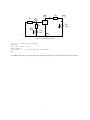
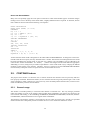
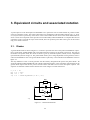
1.3.
Input data example
R3=1.5k
+10V
R1=1k
R2=19k
1.fig
-10V
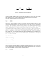
Figure 1.1.: Sample Circuit
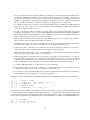
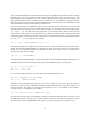
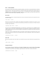
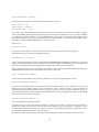
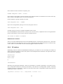
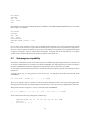
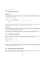
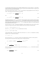
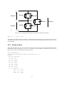
To give the uninitiated some idea of the input data required to accommodate a simple but practical problem,
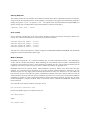
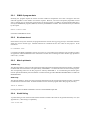
consider the electrical schematic of an inverter circuit shown in figure 1.1. A SCEPTRE version of the circuit
appears in figure 1.2 under the assumption that a transistor equivalent circuit named 2N914A has been stored at
some previous time. The stored model also includes a primary photo current generator. The sample listing given
below will be sufficient to compute the initial conditions that hold before the radiation transient is applied, as well
as the complete transient solution itself , up until 500 nanoseconds of real time. Both printed and plotted outputs
of VR1, VR3, and VCX (a capacitor in the model) will be obtained, plus any other outputs that were requested in
the stored models.
CIRCUIT DESCRIPTION
ELEMENTS
Rl,1-2 = 1
R2,2-4 = 19
R3,5-3 = 1.5
EL,1-5 = 10
ET,4-1 = 10
2
R3
3
R1
5
2
T1
EL=
10 V
R2
4
ET=
10 V
1
2.fig
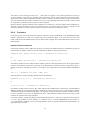
Figure 1.2.: SCEPTRE Version
Tl,2-1-3 = MODEL 2N914A (PERM)
OUTPUTS
VR3, VR1, VCXT1, PLOT
RUN CONTROLS
STOP TIME
= 500, RUN INITIAL CONDITIONS
END
The detailed rules will be given throughout this manual for generating circuit descriptions such as the one above.
3
2. SCEPTRE use
The DC, transient or AC solutions of large electrical networks are computed on request when the circuit description
language described herein is used to convey all the necessary information to the SCEPTRE program. The user is
not required to write the network equations or to possess a knowledge of computer programming. This Section
describes the preparation of circuits and the circuit description language recognized by SCEPTRE.
2.1.
Circuit preparation
The first step taken in using the SCEPTRE program is to prepare an equivalent circuit drawing of the circuit to be
analyzed. The equivalent circuit may consist of resistors, capacitors, inductors, mutual inductance, voltage sources,
and current sources, and/or stored models containing these elements. All of these elements may be linear and/or
nonlinear. Furthermore, most equivalent circuits composed of these elements can be accommodated. This allows
the use of either standard or complex experimental equivalent circuits. The value, or behavior, of any equivalent
circuit element may be defined by a numerical constant, tabular list, or mathematical expression.
After the equivalent circuit has been drawn, each node is given an arbitrary alphanumeric designation consisting
of six characters or less. A node is defined as the point of common potential (voltage) at the junction created by
the connection of two or more network elements.
Next, each component or element in the circuit is given a unique name consisting of not more than five alphanumeric characters. The first character of each element name must be R, C, L, E, or J corresponding to the element
type; i.e., resistor, capacitor, inductor, voltage source or current source, respectively. The letter M is used to designate mutual inductance in the same way. The two exceptions to this are the circuit designation for a stored
model (see subsection 2.3.1) which has no specific rule for its first character, but should be limited to a total of
three alphanumeric characters, and the Convolution model (Appendix A.8), the first character of which is a K. It
is normally very helpful to record on the equivalent circuit diagram the names and nodes chosen. Current flow
directions and source polarities should also be indicated.
The circuit parameter values should be specified in a consistent set of parameter units. Although any consistent
set is acceptable, the system given in table 2.1 is useful for high-speed transistorized circuits. If another system
is desired, the most effective choice is units of voltage, current and time that correspond to the magnitude of
those that are expected in the problems; then determine units of R, L, and C from the fundamental current-voltage
relationships. This choice is always possible in a practical circuit, since the analyst should have some approximate
idea of the range of variables.
In summary, the circuit preparation steps are:
• Draw an equivalent circuit comprising only resistors, capacitors, inductors, and voltage and current sources.
• Assign a name or number to all nodes in the circuit.
• Give a name to each circuit element.
• Assume arbitrary current flow directions in each passive circuit element.
4
Parameter
Resistance
Capacitance
Inductance
Current
Voltage
Frequency
Time
Unit
kΩ
pF
µH
mA
V
GHz
ns
Table 2.1.: Units for High-Speed Transistorized Circuits
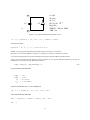
RA
3
R1
4
5
RB
L0
C1
2
JM
6
E1
E2
1
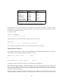
3.fig
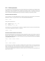
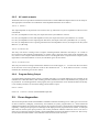
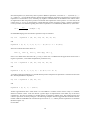
Figure 2.1.: Circuit in SCEPTRE Form
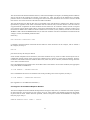
• Indicate the direction of positive current flow in each voltage and current source.
• Choose and record circuit values in a consistent set of parameter units.
Figure 2.1 shows a circuit diagram prepared in the recommended manner.
2.2.
Preparing the SCEPTRE input data
The SCEPTRE circuit description language is a structured free-format language, the syntax of which is easy to
learn and remember. The language consists of descriptive statements constructed syntactically from user-derived
component names, parameter names, node names, and value specifications. These are delimited by special characters such as comma, dash, parenthesis, and equal sign, thereby allowing the program to interpret the statements
properly. Thus, the statements themselves can be punched anywhere on the input data card (columns 1-72) with
any desired spacing. In general, several complete statements can be punched on a card, separated only by a comma.
The rules for continuing a statement from one card to another generally require that the discontinuation be made
immediately after delimiters, with the delimiter appearing as the last non-blank character on the card.
2.2.1.
Headings and subheadings
Networks are described in SCEPTRE language under the following major headings and subheadings regardless of
which mode of analysis is desired.
MODEL DESCRIPTION (INITIAL, PRINT)
MODEL NAME (PERM or TEMP) (NODE-NODE-....NODE)
5
(Comment or message cards, if any, up to 11
ELEMENTS
DEFINED PARAMETERS
OUTPUTS
FUNCTIONS
INITIAL CONDITIONS
CIRCUIT DESCRIPTION
(Comment or message cards, if any, up to 11
ELEMENTS
DEFINED PARAMETERS
OUTPUTS
INITIAL CONDITIONS
FUNCTIONS
RUN CONTROLS
SENSITIVITY
MONTE CARLO
WORST-CASE
OPTIMIZATION
RERUN DESCRIPTION (N)
(Comment or message cards, if any, up to 11
ELEMENTS
DEFINED PARAMETERS
INITIAL CONDITIONS
FUNCTIONS
RUN CONTROLS
CONTINUE
RUN CONTROLS
RE-OUTPUT
OUTPUTS (required)
S/360 only
RUN CONTROLS (optional)
(In the IBM 7090/94 version, no subheadings
heading.)
END
allowed)
allowed)
allowed)
are permitted under this
The MODEL DESCRIPTION heading is used when it is desired to store one or more models. The MODEL name
card, comment cards (optional), and any or all of the five subheadings listed can be used for each model for either
permanent or temporary storage under the MODEL DESCRIPTION heading. One or more models may be entered
under one MODEL DESCRIPTION heading.
The CIRCUIT DESCRIPTION heading is always used when any network is presented for analysis. Any or all of
the ten subheadings listed under the heading may be used.
The RERUN DESCRIPTION heading is used whenever the rerun feature is exercised. All changes to the master
network must appear under this card. Any or all of the five subheadings listed under this heading may be used.
The CONTINUE heading is intended for use only when continued computation is desired after a problem has been
originally run. The only subheading permitted under this heading is RUN CONTROLS. The only other heading
that may appear together with CONTINUE in a run is END.
The RE-OUTPUT heading is used whenever the user desires output from a previously completed run without
repeating that run. No subheadings are permitted under this heading on the 7090/94. The only other heading that
may appear with RE-OUTPUT on the 7090/94 is END. On the S/360, the OUTPUT subheading is required and
the RUN CONTROLS subheading may be used (see subsection 2.6).
6
The END heading is used to terminate every input data deck submitted to SCEPTRE. This heading is the only one
that must always be used without subheadings.
The data supplied within each of the subheadings consists of descriptive statements which are constructed as
properly punctuated sequences of symbols. The group heading, subheading and subsequent statements may be
punched on a card with arbitrary spacing or location from columns 1 to 72. During a single run the user cannot use
all six major headings, although all ten subheadings under CIRCUIT DESCRIPTION could well be used.
Unique sequences of symbols and punctuation are used to convey information in each of the subheadings. A
definition of each of the symbols in the subheadings follows:
Element Name - Denotes the name given to each component (including model circuit designations) of a circuit
(e.g., RA, LLX, E17). No more than five alphanumeric characters may be used to name an element. Model
circuit designations are limited to no more than four alphanumeric characters.
Node - Denotes the designation assigned to each node of a circuit. No more than six alphanumeric characters
may be used to name a node.
Number - A numerical constant that may be written as a signed quantity in either integer or decimal form and
with or without an exponent. Up to 13 characters may be used to represent a number. For example, numbers
may be written in the following forms: 10, 10., 10.0, -.1, -0.1, +1.4, 6.4E9, -74.3E-7, 7E+11, -176.6667E5.
Constant - Same as Number, except a decimal point must be included in the specification of the numerical
constant.
Value - Will be used to denote any of the following: Number, Defined parameter, TABLE, EQUATION, EXPRESSION, or External Function.
Special Value - Will be used to denote any of the following: Value, Constant*Resistor Current, Constant*Resistor
Voltage, Value*Current Source, DIODE TABLE, or DIODE EQUATION (X1, X2).
Variable - Denotes any of the following:
•
•
•
•
•
•
•
The voltage or current associated with any element as VR1, VJ7, IE4, ILM, etc.
Any source or source derivative as J17, DJ17, E4, DE4, etc.
Any defined parameters as P7, DP7, etc.
Any element value as R17, CA, M12, etc.
Time as TIME.
Frequency as FREQ.
Any internal parameter (see subsection 2.2.11).
V Element Name or I Element Name - Denotes the element voltage or current of ELEMENT NAME. For example, the voltage across capacitor CAB1 would be referred to as VCAB1, and the current through inductor
LCHOK would be referred to by ILCHOK.
TABLE Name (Independent Variable) - Used when a variable circuit quantity is given in tabular form. The
table used must be given a unique name prefixed by TABLE or simply T, and followed by a single independent variable in parenthesis. The name may consist of up to five alphanumeric characters. The independent
variable may be any of the quantities defined under VARIABLE, such as TABLE 1A (VC1). If an independent variable, including the enclosing parenthesis is not supplied, then TIME will automatically be chosen.
EQUATION Name (Argument List) - Used when a variable circuit quantity is given in closed form. The equation must be given a name prefixed by EQUATION or simply Q and followed by one or more arguments
separated by commas and enclosed in a parenthesis. The EQUATION name may consist of up to five alphanumeric characters. The argument list may consist of any VARIABLE, CONSTANT, and TABLE (and
its independent variable). For example,
EQUATION 39 (VCX, J2, TIME, TABLE 2 (VC7)).
7
EXPRESSION Name (Math Definition) - This form is an alternative to EQUATION entry that may be used
to describe a variable quantity. It is somewhat more complex than the EQUATION form, but it has the virtue
of needing no further description under FUNCTIONS. The expression must be given a name prefixed by
EXPRESSION or simply X and followed by the mathematical definition. The EXPRESSION name may
consist of up to five alphanumeric characters. It is suggested that numerical designation be used to avoid any
possible confusion with some internal parameters. For example,
X14 (10. * SIN (.628 * TIME)).
Any equation for table must be defined more completely under FUNCTIONS. More detail is given in subsections
2.2.2 and 2.2.6.
The input data deck describing a network is formed simply by punching the heading card and the associated data
sequence for each of the defined data groups.
Remarks such as title, user name, and date may be supplied for output identification purposes by punching the
desired remarks on cards following the CIRCUIT DESCRIPTION card and preceding the first subheading card.
The number of comment cards must not exceed 11, and the entire remark will appear as the title of the output
listing and plots.
The sequence for each of the subheadings in terms of the symbols defined previously are subsequently detailed.
2.2.2.
Elements
This subsection covers the formats required for entering element data into SCEPTRE. The general discussion
pertaining to all elements is followed by four subsections discussing special conditions which pertain to certain
element entries. These subsections cover mutual inductance (subsection 2.2.2), source derivatives (subsection
2.2.2), elements with bounds (subsection 2.2.2), and AC (complex) sources (subsection 2.2.2).
All elements (resistances, capacitances, inductances including mutual, voltage and current sources, source derivatives and model circuit designations) that are to be component parts of the network under analysis must be introduced under this subheading. Entries allowed under the elements subheading are summarized in table 2.2.
Although any combination of alphanumeric characters (maximum 4) can be used for model circuit designations,
names unique from other element names are recommended. Alphanumeric character lengths are listed in table
2.10, subsection 2.2.9. The general form for entries under the ELEMENTS subheading is:
element name, node-node = value
Each network element is defined by stating the element name, the nodes between which the branch is connected,
and the component value. The connection nodes are specified in a from-to order corresponding to the assumed
direction of current flow. The actual tabular values or analytical expressions of elements that are implicitly defined
as variables are specified in subsection 2.2.6. More than one element may be described on a card if the elements
are separated by commas.
Some examples that illustrate proper entries under elements for the constant valued elements of the network of
figure 2.1 are:
E1, 1-2 = 20
E2, 1-6 = 20
JM, 1-4 = 2E1
Note that any of these constant elements may be entered with or without decimal points, or by use of the E format.
Note also that the proper reference direction for voltage sources p p correspond to the direction of current or
positive charge movement within the voltage source.
NOTES to Table 2.2:
8
Name
R
C
L
name
E
J
M name
E name
J name
J name
J name
DE
DJ
Nodes
Value
specification (see note 9)
number
TABLE name (independent variable)
Defined Parameter
, node1 – node2
=
EQUATION name (argument list)
EXPRESSION
name (math. definition)
External Function (argument list)
L name1 – L name2
(see note 1 & 2 and subsection 2.2.2)
Linearly Dependent Sources
, node1 – node2
= constant *VRname
, node1 – node2
= constant *IRname
Primary dependent Current Sources
(see note 3 & 4)
DIODE TABLE name
, node1 – node2
=
DIODE EQUATION (X1, X2)
Secondary dependent Current Sources (see note 4 & 5)
, node1 – node2
= value * Jname †
Voltage and Current Source Derivations (see note 6 & 8)
name
name (see note 7)
R
E
name
J
=
,
,
value (see subsection 2.2.2)
Model Calls (see subsection 2.3)
node1-node2 . . .
= MODEL name . . .
Elements with Bounds (see subsection 2.2.2)
number1 (number2, number3)
node1 – node2
=
number1 (number2)
AC sources (see subsection
2.2.2)
(entry , entry ) ‡
E
(entry , entry ) ,DEGREES
name
, node1 – node2
=
J
(entry , entry ) ,RADIANS
(entry , entry ) ,COMPLEX
Concolution Model Calls
(see
note 10)
FCONVE (constant)
K name
, node1 – node2
=
(see note 11)
FCONVJ (constant)
†: Jname is a primary dependent current source
‡: entry = constant, defined parameter, TABLE name , FREQ
Table 2.2.: Entries under ELEMENTS
9
1. All C,R,L and M entries will be treated as REAL*8 constants in the AC calculations. Before making the AC
calculations, SCEPTRE will evaluate any entries which are given as functions. For example, a capacitor may
be a function of voltage and a resistor may be a function of time. SCEPTRE will evaluate these functions at
TIME=0, using supplied or calculated initial conditions. The appropriate values so obtained will be used in
the AC calculations. Elements as a function of frequency are not permitted in AC calculations.
2. All voltage and current sources which are given as constants (DC sources) or as functions of TIME (Transient
sources) will be given a value of zero in AC calculations, and a WARNING message will be printed out
whenever the argument TIME is used.
3. In order to obtain an AC analysis around a circuit’s DC operating points, the user must either supply Initial
Conditions (see paragraph 2.2.5), or must enter RUN INITIAL CONDITIONS under the RUN CONTROLS
subheading of CIRCUIT DESCRIPTION. If initial condition are supplied, then SCEPTRE determines all
element values dependent on these DC voltages and currents.
4. Primary and secondary dependent current source specifications may be used to represent certain semiconductor junctions when requesting Initial Conditions solutions.
5. By Definition this class of current source can appear only if the appropriate diode source has previously been
included. The secondary source must be specified only as a value times the primary source.
6. Although this entry is permitted in AC calculations, a time-source, and hence its derivatives, are not meaningful. The source will be treated as in Note 2 above and the derivatives ignored.
7. Model circuit designation names can be any combination of no more than four alphanumeric characters.
Names unique from other element names are recommended.
8. If the topology of the circuit dictates that a time derivative is required for a transient analysis (e.g., capacitor
and independent voltage source loop, or inductor and independent current source cut set), then the same is
true for an AC analysis. However, for AC no card entry is required. A time derivative of an AC source means
simply a multiplication by jω. SCEPTRE will detect this situation and will automatically handle it.
9. A complex defined parameter, W, cannot be used as a value specification.
10. Convolution models are either series combination of voltage source and resistor (FCONVE) or parallel
combination of current source and resistor (FCONVJ). See Appendix A.8.
11. The constants in the Convolution Model Call are arbitrarily assigned integers identifying the impedance or
admittance functions stored on Disk 12 as explained in Appendix A.8.
Examples of variable element entries using EQUATION, TABLE or EXPRESSION descriptions are as follows:
El,
E2,
JM,
RA,
LZ,
1-2
1-6
1-4
3-4
1-5
=
=
=
=
=
TABLE 3 (TIME)
EQUATION 47 (VC1, TABLE 2 (ILO),36.)
EQUATION 47 (VC1, P5, 15.)
TABLE 5 (TIME)
EXPRESSION 7 (10. *ILZ + 20.)
The tabular entries for TABLE 3 and TABLE 5, as well as the analytical expression for EQUATION 47 must
be entered under the FUNCTIONS subheading (subsection 2.2.6). A good general rule to follow throughout the
program is that all constants inside parentheses must include decimal points. A more convenient form that always
may be used is to replace the word EQUATION by Q, the word TABLE by T, and the word EXPRESSION by X.
El, 1-2 = T3(TIME)
JM, 1-4 = Q47 (VC 1, P5, 15.)
LZ, 1-5 = 47 (10.*ILZ + 20.)
10
The second and third designations in the SPECIAL VALUE list are intended to accommodate the class of linearly
dependent sources that are encountered in small signal transistor equivalent circuits (see subsection 3.3). The
fourth designation was designed for the class of secondary dependent current sources that always appear in the
large signal Ebers-Moll transistor equivalent circuit (see subsection 3.2). The capability of specially processing
these sources has been built into the program and should always be entered directly in the ELEMENTS section
without parentheses. Examples of these appear in this subsection.
The last two designations in the SPECIAL VALUE list are reserved for primary dependent current sources that
represent diodes or transistor junctions. DIODE EQUATION (X1, X2) would be used when any diode or transistor junction has been entered, and the user wishes to employ the conventional closed form representation
(J = Is (eΘV J − 1)). The value of X1 must correspond to Is in the diode equation, and the value of X2 must
correspond to Θ. The program will automatically use the voltage across that particular current generator as the
independent variable, and for that reason this voltage need not be specified. If for example, a current generator that
is named J18 and is connected between nodes 1 and ground is to be described by the conventional diode equation
as 1 · 10−7 (e30V J − 1), the appropriate entry would be
J18, 1 - GND = DIODE EQUATION (1.E-7, 30.)
Note that decimal points are required for the constants 1 and 30. No further description is required under FUNCTIONS. The designation DIODE TABLE N is used when any diode or transistor junction is to be represented in
tabular form. The independent variable will automatically be taken as the voltage across the current generator.
Therefore, the required entry is simply
J18, 10 - 3 = DIODE TABLE 1
The tabular entries for DIODE TABLE 1 must be entered under the FUNCTIONS subheadings (subsection 2.2.6).
Examples of typical component descriptions that appear in the ELEMENTS group are shown below:
R7, 4-5 = 11.5, E1, GND-1 = 6
JA, 0-4 =
.98 * J18
E12, C-7 = .0005 * VRC
JA is a secondary dependent current source. JK and E12 are linearly dependent sources.
LX3, 9-3 = EQUATION 15X (ILX3,TIME)
Tll, 2-3-7 - MODEL 2N7479AA
Reference to the FUNCTIONS section (Section 2.2.6) is never required for a given entry when the expression
format is used. The rules for the mathematical definition become specialized only in the case when a table is to be
used as an argument. For example, if it is desired to enter capacitor C1 as 10 + 80 * (TABLE 7), where TABLE 7
is a function of VC1, an appropriate entry would be
C1, 7-8 = X314 (10. +80. * XTABLE (T7, VC1))
Note that in this special case the word TABLE is preceded by X and that both the table name, in this case T7, and
the independent variable of the table VC1, must be included in parentheses. Decimal points must always be given
with all constants used in an EXPRESSION. This same entry is given in equation form in subsection 2.2.6.
11
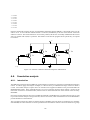
I1
L1
sign
L2
Mutual
Inductance
L3
M12
M13
M23
+
-
I2
I3
4.fig
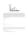
Figure 2.2.: Mutual Inductance Polarities
Mutual Inductance
Mutual inductance is entered according to the general format:
Mname, Lname-Lname = value
If coupling exists between inductors L1 and L2, the appropriate entry must include these elements in place of the
node identification as
MX, L1-L2 = TABLE 1 (IL1)
or
MX, L1-L2 = 32.4
In addition, a physical limitation of the principle of mutual inductance must be observed in order to have a physically realizable circuit. That is, since coefficient of coupling, k, is always less than unity and by definition
k=√
M
<1
L1 L2
√
the user should be certain that M < L1 L2 . Stated in words, the mutual inductance between any two inductors
must be less than the square root of the product of the self-inductances of the components between which the
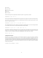
mutual inductance exists. The sign of M is positive if in a given winding the induced voltage of mutual inductance
acts in the same direction as the induced voltage of self-inductance. If the induced voltage of mutual inductance
opposes the induced voltage of self-inductance in a given winding, M is negative. The proper sign for M for the
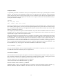
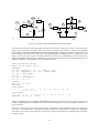
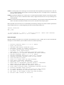
assumed current directions is illustrated in figure 2.2.
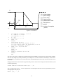
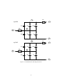
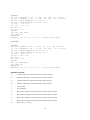
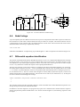
Source Derivatives
The time derivatives of sources must be supplied as input data when certain network configurations are encountered1 . These situations occur whenever a variable voltage source is connected in a loop containing only capacitors
and other voltage sources, and whenever a variable current source is connected in a cut set containing only inductors and other current sources (see figure 2.3).
If the sources in question are constant, the zero derivative will automatically be supplied and the user need not be
concerned. If the user fails to supply a source derivative when one is required, the run will be terminated with an
appropriate diagnostic message. The general form for a source derivative entry is
1 Except
for AC Analysis. See Table 2.2, note 8
12
Capacitor-Voltage Source Loop
C1
E7
C3
Inductor-Current Source Cut Set
L1
J1
C2
L2
L3
5.fig
Figure 2.3.: Configurations That Require Source Derivatives
DEname = value
DJname = value
where the name is that of the appropriate E or J source. An example would be
DERIVATIVE E7 = TABLE 2
or more simply
DE7 = TABLE 2
Elements with Bounds
Three of the DC options, Monte Carlo, Worst-Case, and Optimization require additional information in the entries
under ELEMENTS. For a Monte Carlo calculation, it is necessary to specify parameters for distribution of the
variable elements. For Worst-Case and Optimization calculations, minimum and maximum values of the independent variables must be specified. In all cases, the element information is provided by bounds added in parentheses
after the element values. Except as noted at the end of this paragraph bounds are provided by statements, under
ELEMENTS, of the form
element name, none-node = number (number,number)
or
element name, node-node = number(number)
The first form gives two numbers in parentheses. SCEPTRE reads the smaller number as the lower bound and the
larger as the upper bound. The second form has one number in parentheses. In this form, SCEPTRE reads the
number as the percentage variation allowed in the nominal value of the elements. Examples might be
R2, NZ-N5=12(11,13)
and
R1, N1-NB=6(10)
13
The first example specifies the nominal value of R2 as 12, with lower and upper bounds of 11 and 13, respectively.
The second example specifies that the value of R1 is 6±10%.
For Worst-Case and Optimization, the lower and upper bounds are taken to be the limiting values for the element.
For these calculations, the nominal value must lie within these limits.
For Monte Carlo calculations, the element distribution mean and standard deviation are computed from the lower
and upper bounds as:
mean =
upper bound + lower bound
2
standard deviation =
upper bound − lower bound
6
The exception, mentioned above, to the use of numbers exclusively in specifying elements with bounds is as
follows: Examples with bounds may be specified as values or diode equations if the values or diode equations
are expressed in terms of defined parameters with bounds under DEFINED PARAMETERS. Subsection 2.2.3
describes the allowable format for defined parameters with bounds. An example of an entry under ELEMENTS is
R3, N12-N10=X3(P3+P4)
AC Sources
Source voltages and currents for AC calculations are complex numbers and, therefore, require both real and imaginary parts (or magnitude and phase) for their definition. The format for entering an AC source is:
Ename, node-node = (entry, entry), type
for a voltage source and
Jname, node-node = (entry, entry), type
for a current source. The word entered for ’type’ identifies the meaning of the two entries in the parentheses.
’Type’ may be either DEGREES, RADIANS or COMPLEX. If DEGREES or RADIANS is entered, the first entry
in parentheses is the magnitude, in the polar coordinate expression of the voltage (or current), and the second entry
is phase angle. If type is specified as COMPLEX, the first entry in the parentheses is the real portion of the complex
expression in cartesian coordinates, and the second entry is the imaginary portion. ’Type’ need not be specified. If
it is not, the default value is DEGREES.
An entry, as described above, may be any of the following: constant, the problem frequency (denoted by FREQ),
a TABLE name (where the independent variables must be stated because the default value of the independent
variable is TIME, and the AC calculation takes time as zero), or a real defined Parameter.
The maximum allowed number of independent AC sources is fifty. The maximum number allowed for linearly
dependent AC sources plus secondary dependent AC current sources is also fifty.
The following are examples of AC source definitions:
E1, N1-M3 = (12., 4.), COMPLEX
means that voltage source E1, between nodes N1 and M3, is expressed in complex form as 12+4j volts.
J7, N4-N7 = (T1(FREQ), P6), RADIANS
means that current J7, between nodes N4 and N7, is expressed in polar coordinates, where the magnitude is a
function of frequency to be obtained from Table 1 and the phase angle, in radians, is as specified by P6 under
DEFINED PARAMETERS.
14
2.2.3. Defined parameters
Any variable that can be described in terms of any network variable and/ or any Number may be defined, and this
quantity may be used as an ELEMENT value, an argument in an equation or table, or an output at each time step
of the problem, in the same manner as any conventional output. Examples of the use of this feature are given in
Section 4. More than one defined parameter may be entered on a card if they are separated by commas.
Real Valued Defined Parameters
The input format for real-valued defined parameters requires that the first letter be P followed by no more than five
alphanumeric characters. The general form for entries under DEFINED PARAMETER IS:
Pname = value
Some possible combinations are:
PWR = EXPRESSION 69 (IE 3 * E3)
P2 = TABLE 1 (VC7)
PX7 = EQUATION 2 (VC7, VR1)
For the special case in which the derivative of a quantity is supplied, the first two letters must be DP followed by
no more than four alphanumeric characters, or in general
DPxxxx = value
Real-Valued Defined Parameters with Bounds
Real-valued defined parameters with bounds may be used as independent variables in DC calculations (under the
MONTE CARLO, WORST-CASE or OPTIMIZATION subheadings of CIRCUIT DESCRIPTION, see subsection
2.2.8). When independent variables are used in this manner, they must be specified with bounds under DEFINED
PARAMETERS. The format is:
Pname = number (number, number)
or
Pname = number (number)
The first form gives two numbers in parentheses. SCEPTRE reads the smaller number as the lower bound and the
larger as the upper bound. The second form has one number in parentheses. In this form, SCEPTRE reads the
number as the percentage variation allowed in the nominal value of the independent variable.
For Worst-Case and Optimization calculations, the nominal value must not lie outside of the region defined by the
upper and lower bound.
15
Real-Valued Defined Parameter Total Differentials
The user must specify the closed form differentials for each defined parameter that is used as a dependent variable in
adjoint calculations (Optimization, Sensitivity, and Worst-Case). The defined parameter must be a function of one
or more dependent variables and zero or more independent variables. Valid dependent variables and independent
variables for these calculations may be found in table 2.7 and table 2.8. The user should enter differentials of
defined parameters under the DEFINED PARAMETERS subheading of CIRCUIT DESCRIPTION.
For a defined parameter, Pname, the total differential is given by
GPname = list
’List’ is a sum of products of the form PX*DY, where PX is a defined parameter representing the partial derivative
of the dependent variable with respect to an independent variable, and DY is the differential of the independent
variable.
Example 1:
DEFINED PARAMETERS
..............
PABC = X1 (IRL**2+ILA**2)
GPABC = P2*DIRL+P3*DILA
P2 = X2(2.*IRL)
P3 = X3(2.*ILA)
Example 2:
DEFINED PARAMETERS
................
PEX = XA(VC1**2+(IR1*R1)**2)
GPEX = PA*DVC1+P3*DIR1+P4*DR1
PA = X2 (2*VC1)
P3 = X3(2.*IR1*R1**2.)
P4 = X4(2.*R1*IR1**2.)
Complex Valued Defined Parameters
Complex valued defined parameters are used to enable complex outputs from the AC analysis portion of the
program. Complex valued defined parameters are analogous in principle to the real valued defined parameters,
designated with a P. The appropriate prefix for the complex valued defined parameter is W, followed by no more
than five alphanumeric characters. Unlike the real valued defined parameter, P, a complex valued defined parameter,
W, cannot be use to define elements; that is, it cannot appear in an equation, expression, table or function.
The acceptable entries, under the heading DEFINED PARAMETERS, are
Wname = real value defined parameter
Wname = TABLE name
Wname = EQUATION name
(see subsection 2.2.6 for the correct way to distinguish the real and complex valued arguments.) Also
16
Wname = EXPRESSION name
(see subsection 2.2.6 for a list of the more general FORTRAN complex operational functions available.) Also
Wname = external function
(It is the user’s responsibility, when writing FORTRAN programs, to insure the correct declaration and usage of
complex valued quantities.)
Alternatively, the format allowed for specifying AC sources can be used. This format is
Wname = (entry, entry) type
where the details are described in subsection 2.2.2.
2.2.4. Outputs
Tabular Form
Any output must consist of some dependent variable which is a function of some independent variable. SCEPTRE
outputs consist of printed tabular listings of requested dependent variables as functions of time and/or plots of the
dependent variables as functions of time or some other independent variable. In SCEPTRE, the following general
quantities may serve as either dependent or independent variables:
• The voltage or current associated with any passive element as VR1, IL6.
• The voltage or current associated with any source as E1, IE1, J2, VJ2.
• Any element value as C17.
• Any transient state variable derivative as DC4, DL13B.
• Any Defined Parameter as P12.
• Any Complex Valued Defined Parameter (Wname) in AC Calculations.
• Any Defined Parameter derivative as DP12 if the user has supplied one.
• Any internal parameter as defined in table 2.11.
All requested outputs in SCEPTRE will be supplied in printed tabular form. The general format for requesting
printed outputs is:
variable, variable, variable
and/or
variable
variable
variable
Note that no output request card ever ends with a comma.
17
Plotted Form
In addition, the user has the option of requesting plotted outputs for any or all quantities. If plotted outputs are
desired, the word PLOT is used as the last entry on each output request card for which plots are desired. The
general format is:
variable, variable, PLOT
and/or
variable, PLOT
variable, PLOT
Some typical output requests follow:
VR3, IR3, VR2
VR5, VC29
VRY, VC1, ESUP, PLOT
IC8
Note that more than one output can be requested on a single card. The third card indicates that three quantities are
required and that all three are to be plotted as well as printed. The quantity, IC8, (the current through capacitor C8)
would be output in printed form only. If the word PLOT is used, no other dependent variable may follow it on that
card.
All indicated variables in the above example will use time as the independent variable. If a different independent
variable is desired for the plotted form, the following format must be used.
IC14, PLOT (VC14)
In this case, the current through capacitor C14 would be plotted as a function of the voltage across it. The printed
output would be IC14 as a function of time.
Additional flexibility is available to permit the user to attach a different label to any output quantity except TIME.
Consider that elements C1 and R7 exist in a given network and that the voltage across both (VC1 and VR7) are of
interest. If the user decides to rename them as VIN and VOUT, the outputs may be requested as VC1 (VIN), VR7
(VOUT), PLOT. All renames must be limited to six alphanumeric characters and the first character may be any
alphanumeric character. The plot, rename, and choice of independent variable options can be presented in terms
of the general format as:
yqty(ylabel),......,
PLOT(xqty(xlabel))
If no rename is desired, the general format reduces to
yqty, ......, PLOT (xqty)
If, in addition, only time is desired as the independent variable, this can be further reduced to
yqty,........,
PLOT
And, if no plotted information is desired, the simplest form arises as
yqty, ....
18
Composite Plots
A specialized plot format is available in which up to nine dependent variables may be plotted against a common
abscissa. The ordinate for each dependent variable runs across the page and is separately scaled, and unique
graphic characters are used to represent each quantity. Use of this feature requires that all of the quantities which
are to be plotted together may be requested on the same card or sequence of cards under OUTPUTS followed by a
specific plot name. For example,
OUTPUTS
VC1, VC2,P13, PLOT
VR11, VCET1, JET6, IE4, PLOT 1
In this case, quantities VC1, VC2 and P13 would be plotted singly, as usual. Quantities VR11, VCET1, JET6, and
IE4 would be plotted together, since they have been requested together with a plot that has been ’named’ simply
as 1. Any plot name may include up to six alphanumeric characters and more than one name may be used to plot
different combinations of quantities.
The composite plot feature also requires a PLOT INTERVAL entry under RUN CONTROLS. While this is a RUN
CONTROL entry, it is discussed here because it relates only to composite plots, and its omission will cause the
requested plots to appear in their usual separate formats.
The physical length of any composite plot may be controlled. The number of pages encompassed by the abscissa
(independent variable) is determined by the problem duration (STOP TIME) and a user supplied entry called
PLOT INTERVAL. The former divided by the latter will determine the number of lines required which will, in
turn, determine the number of pages required. For the system S/360, 66 lines will fill one page. Therefore, a
problem duration of 1000 and a PLOT INTERVAL of 5 will require 1000/5 = 200 lines, or three pages, plus two
lines on a fourth page (plus approximately three lines per variable for identification and scaling information). The
PLOT INTERVAL entry always appears under RUN CONTROLS, and the format is simply:
PLOT INTERVAL = number
Only one PLOT INTERVAL will be recognized regardless of the number of composite plots that are requested.
For additional discussion of composite plots, see Appendix A.5.
Convolution Outputs
The above discussion about outputs also applies to transient runs employing the Convolution option. One precaution is noted here. When the user requests an element of a Convolution model as output, he must prefix its name
Kname (see table 2.2) with a letter denoting the element desired. The code is as follows:
E for the voltage source of an impedance kernel; e.g., EKname
J for the current source of an admittance kernel; e.g., JKame
R for the resistance value of a kernel; e.g.. RKname
Additional prefixes, I and V, are required if the user is requesting currents and voltages of these elements; e.g.,
IEKname, IRKname, VJKname, VRKname. See subsection 4.6 for a discussion of Convolution kernels.
19
AC Outputs
The results of AC calculations can be obtained as outputs in either tabular or plotted form. The general rules for
output requests given in subsections 2.2.4 and 2.2.4 apply equally to AC outputs, except that AC outputs are not
given as functions of time. All AC tabular outputs and all but one type of plot are given as functions of frequency.
The Nyquist plot gives the imaginary part of a complex function vs. the real part.
The standard forms of requests, under OUTPUTS,
variable, variable, variable
and/or
variable
variable
variable
will produce a tabular printout of magnitude vs. frequency, and phase in degrees vs. frequency for each variable.
This is the default entry. The word DEGREES is optional. If the output is desired in radians, the proper entry is
variable, variable, RADIANS
The entry
variable, COMPLEX
produces a printout of the real part of each variable vs. frequency and the imaginary part vs. frequency.
If the word PLOT is added to the entry
Variable, COMPLEX, PLOT
a plot of the same data is also obtained, as described in subsection 2.2.4.
The Nyquist plot shows the imaginary part vs. the real part for each variable. The proper entry for the Nyquist plot
is
variable, variable, NYQUIST, PLOT
In this entry only the word PLOT is optional. Both the plot and the printout will appear if the word NYQUIST
appears in the entry.
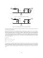
2.2.5. Initial Conditions
The complete solution of the general transient analysis problem requires that all independent initial conditions be
supplied. The set of all capacitor voltages and inductor currents that exist at the start of the problem are sufficient
for this purpose. These may be supplied by the user or computed by the program.
20
L5
7
+
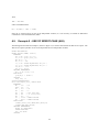
8
C11
4
5
6.fig
Figure 2.4.: Voltage Polarity and Current Direction
Manual Initial Conditions
This section is usually superfluous if the run is being made in either the initial conditions only, or the automatic
initial conditions mode, since the initial conditions will be computed by the program in these situations.
When initial conditions are supplied by the user, the format it
VC.... = number
IL.... = number
Initial capacitor voltages and inductor currents may be supplied by simply listing the desired values. Any initial
conditions not specified will be taken as zero. If all initial conditions are zero, neither the heading card nor the data
are required. Care must be taken to establish the proper polarities for initial conditions. Initial inductor currents
are positive if they flow in the same direction as the assumed current direction for the inductor. Also, the initial
capacitor voltages are positive when they are consistent with the assumed voltage polarity for the capacitor.
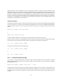
The assumed current direction through inductor L5 of figure 2.4 is from node 7 to node 8. If the initial inductor
current is in this direction, it is entered under the INITIAL CONDITIONS subheading as a positive quantity. If,
however, the current flows in the other direction, it is preceded by a negative sign. The same convention applies
to the capacitor, where the assumed positive sense of the voltage is associated with the tail of the reference arrow
(node 4 in figure 2.4). If the actual initial voltage polarity agrees with the arbitrarily chosen reference direction,
that initial voltage is entered as positive; if not, it is entered as negative. Proper statements for the example of
figure 2.4 are, under ELEMENTS:
L5, 7-8 = value
and either of the following:
C11, 4-5 = value
C11, 5-4 = - value
Automatic Initial Conditions
When the user requests that initial conditions be calculated by the program (see subsection 2.2.7), he need supply
no initial conditions himself. To shorten the initial condition calculation, however, he may supply approximations
of the voltages across diodes or transistor junctions. The language must be
VJ....
= number
21
The iterative process will begin with any VJ.... entries that are supplied. One practical application of this type
of input would be to bias the ON and OFF sides of symmetric circuits such as flip-flops in the desired state.
Approximate values could be supplied and the DC solution would then provide the correct voltages for the desired
state. The results of the DC solution would then carry over to the beginning of the transient solution if one is called
for. Appendix A.3 discusses special options in initial conditions.
NOTE: If the user requests automatic initial conditions for a transient run, and also supplies initial conditions for
capacitor voltages and inductor currents per subsection 2.2.5, his supplied values can appear as impulses at the
start of the transient run. This situation can lead to erroneous results. See [2, subsection 2.4.1].
2.2.6. Functions
In this data group, each of the tables and equations referred to under ’ELEMENTS’ and ’DEFINED PARAMETERS’ (subsections 2.2.2 and 2.2.3, respectively) must be defined in detail. If no such references have been
made, neither the FUNCTIONS heading card nor data need be supplied. The equation definition sequence will be
discussed first.
Equation Definition Sequence
Each unique equation (used to define the variation of an element or defined parameter) is defined by giving the
equation name, a dummy variable list, and the mathematical definition. The general format is
EQUATION name (Dummy Variable List) = (Mathematical Definition)
or
Q name (Dummy Variable List) = (Mathematical Definition)
The dummy variable list must contain the same number of entries as does the argument list in the original equation
reference. Each dummy variable may contain up to six alphanumeric characters, the first of which must not be a
number or the letters I through N inclusive. For example, if an equation has been referenced under ELEMENTS
as:
LX3, 9-3 = EQUATION 15X (ILX3, TIME, VC1)
then this equation could be explicitly defined under FUNCTIONS as:
EQUATION 15X (A, B, C) = (Mathematical Definition)
or
Q 15X (A, B, C) = (Mathematical Definition)
The dummy variables in this case are A, B, C which replace ILX3, TIME and VC1, respectively. The mathematical
definition itself must be included in parenthesis and must be written in terms of A, B, C, along with any constants
and allowable subprogram functions that apply. It is important to mention that there would be no need for the user
to reserve quantities A, B, and C for equation 15X alone. These dummy variables may be freely used in other
equations to represent other circuit quantities.
As another example, consider the equation mentioned in subsection 2.2.2, where it was desired to enter capacitor
C1 as 10 + (80) (TABLE 7) where TABLE 7 is a function of VC1. If, under ELEMENTS, the user enters C1,
7-8 = EQUATION 2 (TABLE 7 (VC1)), then EQUATION 2 must be explicitly defined under FUNCTIONS. An
appropriate entry would be:
22
EQUATION 2 (A) = (10. + 80.*A)
At each solution pass, the ordinate value of TABLE 7 would replace the dummy variable A and the computation
10. + 80.*A would be carried out. Note that decimal points are required for the constants 10 and 80 because they
appear with an EQUATION designation.
Still another method can be used that is particularly efficient when more than one equation of the same general
form is used in a given run. Let it be desired to enter C1 as in the above paragraph, in addition to C2 as 5 + (120)
(TABLE 4) where TABLE 4 is a function of VC2. Under ELEMENTS the user may enter two cards as:
C1, 7-8 = EQUATION 2 (10.,80., TABLE 7 (VC1))
C2, 6-1 = EQUATION 2 (5.,120., TABLE 4 (VC2))
and under FUNCTIONS Equation 2 is explicitly described as
EQUATION 2 (A, B, C) = (A+B*C)
At each solution step, C1 is evaluated in the program by replacing dummy variables A, B and C by 10., 80., and
the ordinate value of TABLE 7, respectively. C2 is then evaluated by replacing A, B, and C by 5., 120., and
the ordinate value of TABLE 4, respectively. Note that two quantities of the same mathematical form have been
accommodated by one equation.
The mathematical Definition may be any combination of the allowable operations, functions, or variables. The
following mathematical operations and corresponding symbols are included in SCEPTRE:
Operation
Exponentiation
Multiplication
Division
Addition
Subtraction
Symbol
**
*
/
+
-
The order in which operations are performed is indicated by the order in which the operators are listed. The use
of parentheses, to denote clearly the intended mathematical combination is suggested to avoid ambiguity. For
example, X+Y*Z should be written as (X+Y)*Z if X+(Y*Z) is not intended.
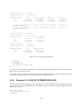
Any function of real arguments that is available in the FORTRAN IV Subprogram Library may be use in any
EQUATION or EXPRESSION. A few of the most widely used of these are listed below. In addition, the functions
of complex Arguments listed in table 2.3 may be used.
The argument of any function may be any allowable mathematical definition. In addition, the user may supply
subprogram functions that he has written himself (see subsection 2.7). When these functions are referenced by an
EQUATION, all variables that appear as the arguments of operational functions must be given in terms of dummy
variables. Mathematical definitions are not limited to 72 characters (one card) and may be continued on subsequent
cards, using as many as necessary.
Double precision entry names for FORTRAN subprogram functions must be used. Thus, the first character for each
entry name of any FORTRAN library subprogram must be D, as DLOG or DSIN. Consult IBM System/360 FORTRAN IV Library Subprograms, FORM C28-6596 for available functions. User written FORTRAN subprogram
functions must be typed double-precision.
For AC calculations, complex defined parameters (see subsection 2.2.3) may be entered using equations, if desired.
In this event, the argument list may contain both real and complex valued terms. (The complex entries are indicated
23
Function
Real Arguments Complex Arguments
Square root
DSQRT
ZSQRT
Sine
DSIN
ZSIN
Cosine
DCOS
ZCOS
Exponential
DEXP
ZEXP
Arctangent
DATAN
—
Absolute value
DABS
DZABS
Natural logarithm
DLOG
ZLOG
Common logarithm DLOG10
—
Each symbol is followed by an argument in parenthesis.
Trigonometric functions require the argument in radians.
Table 2.3.: Functions of Real and Complex Arguments
by the prefix E, J, V, or I only. No argument of any equation may use the prefix W). Therefore, in order to correctly
distinguish between real and complex arguments internally, the letter Z has been reserved as the prefix to indicate
all complex valued dummy arguments.
For example: Under
DEFINED PARAMETERS
W = Ql (3., VR2, P3, T1, IL3)
and VR2 and the IL3 would denote complex valued arguments. Then, under
FUNCTIONS
Q1 (A, Z1, B, C, Z2) = (mathematical expression)
where the dummy arguments Z1 and Z2 are used in place of VR2 and IL3, respectively.
Tabular Definition Sequence
Every TABLE name that has been referenced under ELEMENTS or DEFINED PARAMETERS must be explicitly
defined under the FUNCTIONS subheading. The general format is
TABLE name, number, number.......
number
or
DIODE TABLE name, number, number, .... number
Acceptable variations of this format are shown in the examples following figure 2.5.
Note that the designations TABLE 1 and DIODE TABLE 1 refer to the same table; therefore, these may not be
used to name two different tables in any run. The tabular data itself is represented by a series of numbers in
pairs, separated by commas, in which the number representing the independent variable point comes first with the
dependent variable point following.
Note that as figure 2.5 suggests, any number of point pairs can be supplied per card. The data pair points must be
supplied such that the independent variable is in increasing algebraic order. No specific limit to the number of point
24
TABLE ERIN
value
2
1
TIME
1
7.fig
2
3
4
Figure 2.5.: TABLE ERIN Values as a Function of Time
pairs that may constitute any table is defined. Only single value functions are allowed. It is permissible to supply
two consecutive independent-variable values that are equal, but which have different dependent variable values.
This may be done to produce step functions as illustrated in figure 2.5. When the table values are updated at each
solution time step, linear interpolation is used between the points supplied. For independent variable values falling
outside the range of values supplied in table, linear extrapolation is performed to determine the correct table value
and, therefore, proper termination may be necessary. For example, in figure 2.5, for any value of TIME in excess
of 3, the dependent variable ERIN will be assigned the value zero because of the use of the point pair 4, 0. When
the independent variable takes on a value exactly at a step point, the ordinate used depends upon the direction from
which the step was approached.
TABLE ERIN
0, 0
1, 1
2, 1
2, 1.5
3, 1.5
3, 0
4, 0
or
TABLE ERIN
0, 0,1, 1 , 2, 1, 2, 1.5, 3, 1.5,
3, 0, 4, 0
or
TERIN = 0, 0, 1, 1, 2, 1, 2, 1.5, 3, 1.5, 3, 0, 4, 0
In situations where the same table will serve to define more than one quantity, the user need only explicitly define
the table once. A common situation occurs when two current generators in the network are defined by the same
tabular data, differing only in the independent variable. In this case the user may define both generators under
ELEMENTS as:
J1, 1-2 = TABLE 1 (VC1)
J2, 7-8 = TABLE 1 (VC2)
Under FUNCTIONS, the user would define TABLE 1 only once.
25
2.2.7. Run controls
This subsection contains all the auxiliary information needed to control the run. The information does not directly
affect the network. Most of these quantities have automatic default entries that hold unless specific entries are
supplied by the user. The default entries are given in table 2.4. All possible entries under the RUN CONTROLS
subheading are given in the following subsections. These entries may be made in any order, and as many may be
placed on a card as will fit, if they are separated by commas.
Run Limits
All transient runs must have a problem duration in the time units consistent with those used to describe the circuit.
The form is simply:
STOP TIME = number
Since the user will never know in advance the computer time required for the solution of a given run, it may
sometimes be desirable to enter a limit that will automatically terminate the run if that limit is exceeded. The limit
in minutes may be entered as
COMPUTER TIME LIMIT = number
The preset value for COMPUTER TIME LIMIT is set to 600 minutes. This statement is active on IBM System/360
computers where a system clock is installed and applies to total elapsed time. It should be noted that for operation
under OS/MVT the time used for the above statements is elapsed time as accumulated on the system clock and not
CPU utilization time.
Another type of limit is available that operates on the number of passes made by the integration routine. In the
absence of any instruction from the user, the program imposes a limit of 20,000 passes. The user may change this
limit by entering.
INTEGRATION PASSES = number
Start Time
Most transient problems start at time equal to zero, and this entry may be omitted. Otherwise, the appropriate entry
is:
START TIME = number
Integration Routine
Four integration routines are available for use with S/360 SCEPTRE. Three are explicit (XPO, TRAP and RUK)
and one is implicit. (Implicit is not available on 7090/94.) The default option is XPO and, therefore, this method
is used unless one of the others is specifically requested. When one of the others is desired, the format is
INTEGRATION ROUTINE = TRAP
26
Quantity
STOP TIME
COMPUTER TIME LIMIT
MAXIMUM INTEGRATION PASSES
START TIME
INTEGRATION ROUTINE
MINIMUM STEP SIZE
Default Information
None
None (7090/94), 600 min (S/360)
20,000
0
XPO
1 · 10−5 (STOP TIME) xpo, trap, ruk
1 · 10−14 (STOP TIME) implicit
MAXIMUM STEP SIZE
2 · 10−2 (STOP TIME)
STARTING STEP SIZE
1 · 10−8 (STOP TIME) xpo, trap,ruk
1 · 10−8 (STOP TIME) implicit
XPO TRAP RUK
IMPLICIT
MINIMUM ABSOLUTE ERROR
.0001 .00005 .00005 .0001
MAXIMUM ABSOLUTE ERROR
.005
.001
.005
MINIMUM RELATIVE ERROR
.0002 .0005
.00005
MAXIMUM RELATIVE ERROR
.005
.01
.005
Mode of Analysis
Transient Only
NEWTON-RAPHSON PASS LIMIT
100
RELATIVE CONVERGENCE
0.001
ABSOLUTE CONVERGENCE
0.0001
MAXIMUM PRINT POINTS
1000
COMPUTER SAVE INTERVAL
15
VECTOR EQUATIONS
100 (transient) 70 (DC)
XPLOT DIMENSION
10
YPLOT DIMENSION
5
TYPE FREQUENCY RUN
LINEAR
NUMBER FREQUENCY STEPS
10
COMPRESSION COUNT
.3*(Input Function Buffer)
RUN MONTE CARLO †
10
INITIAL RANDOM NUMBER
127263527
DISTRIBUTION
GAUSSIAN
RUN OPTIMIZATION †
30
MINIMUM FUNCTION ESTIMATE
0
OPTIMIZATION CRITERION
10−7
OPTIMIZATION RANDOM STEPS
0
RANDOM STEP SIZE CONTROL
.2
INITIAL H MATRIX FACTOR
1.
RUN WORST CASE †
NOMINAL
†: Default value obtains when Run Control is entered without ’=number’.
If the Run Control itself is omitted, the indicated calculation will not occur.
Table 2.4.: Default run control quantities in SCEPTRE
27
or
INTEGRATION ROUTINE = RUK
or
INTEGRATION ROUTINE = IMPLICIT
Certain additional operations are required when implicit integration is used. These are performed internally according to a prescribed default mechanism, but the user may exercise control over the default. (See [2, subsection
5.5].) Two possible statements are available.
USE DIFFERENCED JACOBIAN
USE SYMBOLIC JACOBIAN
Use of the Convolution routine requires that the RUK integration routine be specified.
Minimum Step Size
Any transient run will automatically terminate whenever a time step size is required that is smaller than the minimum step size. If this quantity is not supplied, the program will automatically compute a minimum limit. For
explicit integration, this minimum limit is equal to 1 x 10⁻⁵ times the problem duration (STOP TIME). For implicit integration, the multiplying factor is 1 x 10⁻¹⁴ . If a specific minimum step size independent of the problem
duration is desired, the format is:
MINIMUM STEP SIZE = number
For example if, in a run using explicit integration,
STOP TIME- = 5000
is specified, the minimum size would automatically be 0.05. To change this to 0.01, use
MINIMUM STEP SIZE = 0.01
Maximum Step Size
This quantity sets an upper limit to the time solution increment that can be used to prevent a complete transient
solution composed of few solution points. If this quantity is not supplied, the program will automatically compute
a maximum limit equal to 2 x 10⁻² times the problem duration (STOP TIME). If a specific maximum step size
independent of the problem duration is desired, the format is:
MAXIMUM STEP SIZE = number
28
Starting Step Size
This quantity will be the size of the first time solution increment that is taken. Subsequent increments are automatically chosen by the integration routine. If this quantity is not supplied, the program will automatically compute a
starting step equal to 1 x 10⁻³ for explicit, 1 x 10⁻⁸ for implicit, times the problem duration (STOP TIME). If a
specific starting step size independent of the problem duration is desired, the format is:
STARTING STEP SIZE = number
Error Criteria
Unless otherwise specified, any of the three explicit integration routines will operate with preset relative error
criteria. If it is desired to modify these criteria, the proper formats would be:
MINIMUM
MAXIMUM
MINIMUM
MAXIMUM
ABSOLUTE
ABSOLUTE
RELATIVE
RELATIVE
ERROR
ERROR
ERROR
ERROR
=
=
=
=
number
number
number
number
The only error criterion that pertains to implicit integration is MINIMUM ABSOLUTE ERROR. The SCEPTRE
integration routines are described in detail in [2].
Mode of Analysis
SCEPTRE can compute DC, AC, or transient solutions only, or certain combinations of these. The combinations
are DC with AC and DC with transient. Runs combining AC with transient cannot be made. The default mode
of analysis is the transient run; that is, unless otherwise specified by the user, only the transient solution will be
computed. The transient solution can be run with or without convolution (see Appendix A.8).
SCEPTRE offers five DC solution modes: Initial Conditions, Sensitivity, Monte Carlo, Worst-Case and Optimization. Any of the five may be used alone, or as a source of initial conditions data for a Transient or AC run.
Alternatively, the user may supply initial conditions data himself as entries to a Transient or AC run without the
help of the DC options. One of the DC options, called Initial Conditions, takes part in all DC solutions. It may be
called separately, and if any other DC option is called, that option uses two or more passes of the Initial Conditions
calculation to produce its results. The Initial Conditions solution (and thus the other DC options) may use either
the Newton-Raphson or implicit method. Table 2.5 shows the entries, under RUN CONTROLS, used for each
mode of analysis.
If it is desired to run only DC solutions, the proper entry is:
RUN INITIAL CONDITIONS ONLY
plus the selected DC option, for which the entries are:
RUN SENSITIVITY
and/or
RUN MONTE CARLO
29
Mode of Analysis
Desired
DC Solutions
only
DC Plus Transient
DC Plus AC
Transient only
AC Only
Transient
Plus
AC
RUN CONTROL Required
RUN CONTROL Optional
RUN INITIAL CONDITIONS ONLY
RUN IC VIA IMPLICIT
RUN SENSITIVITY
RUN MONTE CARLO
RUN WORST CASE
RUN OPTIMIZATION
RUN IC VIA IMPLICIT
RUN INITIAL CONDITIONS or one or more
of the following
RUN SENSITIVITY
RUN MONTE CARLO
RUN WORST CASE
RUN OPTIMIZATION
plus STOP TIME = number
same as above plus RUN AC
STOP TIME = number
RUN AC
This combination is not possible
Notes
1
2
2
2
2
1
2
2
2
2
RUN IC VIA IMPLICIT
1
3
Table 2.5.: Run controls for specifying mode of analysis
and/or
RUN WORST CASE
and/or
RUN OPTIMIZATION
(See subsection 2.2.7 for more detailed discussion of the Sensitivity, Monte Carlo, Worst-Case and Optimization
Run Controls.)
Any one or more of the above five entries will cause Initial Conditions to be found by the Newton- Raphson
method. If it is desired that the DC solutions be run using the Implicit technique, include the extra entry
RUN IC VIA IMPLICIT
(See Appendix A.3 for a discussion of the Implicit Method of computing Initial Conditions.)
Notes:
1. The entry RUN IC VIA IMPLICIT will cause all requested DC solutions to use the implicit methods. If this
card is not entered, all requested DC solutions will be by the Newton-Raphson method.
2. DC solutions are accomplished in the order shown in this table. See text.
3. Transient only is the default mode of analysis.
30
The user should note that the method he chooses, either Newton-Raphson or Implicit, for finding Initial Conditions
will be used in all DC solutions he requests on the same run. Thus, the choice of the method for a particular
problem can have a sizeable effect on running time when several DC calculations are involved. The user should
thus exercise care in the selection of the Initial Conditions method.
The user should also note that the DC runs are performed in the order Sensitivity, Monte Carlo, Worst-Case and
Optimization, regardless of the order in which the cards are entered. Thus, if the user desires to use the results of
any particular DC computation as initial conditions for the transient or AC solution to follow, he must not request
any of the DC options which appear after it in the above mentioned order. For instance, if the user wishes to use
the results of a Monte Carlo solution as initial conditions for a transient (or AC) solution, he must not enter a RUN
WORST CASE or RUN OPTIMIZATION card, or these DC solutions will remove the Monte Carlo data from the
voltages, currents, and defined parameter tables.
If the entry
RUN INITIAL CONDITIONS ONLY
is omitted, a transient solution will follow the DC solutions. If the user desires an AC analysis, with or without a
DC analysis, the entry is:
RUN AC
plus entries for any DC analysis desired.
Under normal computational circumstances, the initial conditions for any rerun are either inserted by the user or
computed by the DC portion of the program (see subsections 2.4.1 and 2.4.2). There may be situations, however,
in which it is desirable to have the results of master runs, either AC, DC or transient, used as the starting values for
one or more associated reruns.
If it is intended that all associated reruns use the final values of the master run as initial conditions, the appropriate
entry under RUN CONTROLS is:
IC FOR RERUNS = MASTER RESULTS
If it is intended that each rerun use the final result of the preceding rerun in the sequence, the entry is:
IC FOR RERUNS = PRECEDING RESULTS
(See Appendix A.3 for additional information.)
Convergence of the Newton-Raphson Routine
The Newton-Raphson iteration method should produce convergence and, hence, d-c solutions in less than 30 passes
for most networks. If convergence is slow or does not occur, some realistic limit should be placed on the number
of passes that are made. Unless otherwise specified, a limit of 100 passes is built into SCEPTRE. To change this
limit, the proper entry is:
NEWTON-RAPHSON PASS LIMIT = number
31
Convergence is considered to have occurred if
|Y (n) − Y (n − 1)| ≤ A ∗ |Y (n)| + B,
where Y refers to the vector of initial condition state variables, n is the number of completed passes, A is the
relative criterion, and B is the absolute criterion. The values A = 0.001, B = 0.0001 are built into SCEPTRE. The
user probably will not want to change these values, but if either quantity is to be changed, the proper entries are:
RELATIVE CONVERGENCE = number
ABSOLUTE CONVERGENCE = number
Output Control
Some transient runs may require thousands of solution points, and it is usually unnecessary to have every solution
printed out. SCEPTRE is processed to output a maximum of 1000 spaced points regardless of the number of steps
taken. The maximum number of printed output points may be changed for any particular run by entering:
MAXIMUM PRINT POINTS = number
An additional means exists by which the number of solution points may be precisely controlled and chosen more
selectively. The user supplies the desired time interval and only those solution points that fall on or immediately
after integer multiples of the specified interval will be printed in this series. The required entry is;
PRINT INTERVAL = number
This printed series will appear in addition to the normal printed output format. If only this printed series is desired,
the normal printed output format may be suppressed by the entry:
MAXIMUM PRINT POINTS = 0
(For additional discussion of print interval, see Appendix A.4.)
A discussion of the PLOT INTERVAL run control, used to control the length of composite plots may be found in
subsection 2.2.4.
Automatic Termination of Transient Runs
The user may often desire to monitor certain voltages or currents in a network to determine their relation with some
predetermined quantity. If the relations are satisfied, there may be no further interest in continuing the run. The
run can be terminated at that point by the entry:
TERMINATE IF (XXXXXX relational operation XXXXXX)
The X quantities refer to any variable or constant. The user frequently supplies some element voltage or current
for this purpose. The following relational operators may be used:
.LE. less than or equal to
32
.LT. less than
.GT. greater than
.GE. greater than or equal to
.EQ. equal to
.NE. not equal to
NOTE: Decimal points are required before and after an operator. A typical entry would be:
TERMINATE IF (VCC .GT. 0.)
which would automatically terminate that particular run whenever the voltage across capacitor CC became positive.
The termination feature may be extended to cover AND/OR logical situations by using the logical operators .AND.
and .OR.. A legal entry could be:
TERMINATE IF ((VCC .GT. 0.) .OR. (IL17 .GE. 7.))
This would terminate the run if the voltage across capacitor CC became positive or the current through inductor
L17 exceeded 7 units of current. The other logical possibility would be simply
TERMINATE IF ((VCC .GT. 0.) .AND. (IL17 .GE. 7.))
All automatic Termination conditions must apply to all reruns that are associated with a given master run (see
Section 2.4.1). One variation is available. If it is desired that all remaining reruns be canceled if a termination
condition is met, the word STOP is used instead of TERMINATE. Then a typical entry would be:
STOP IF (VCC .GT. 0.)
Computer Save Interval
Particularly long computer runs should be protected against complete loss arising from improper termination
caused by electrical malfunction, operator error, etc. This is done by periodically recording the status of the
run on tape such that it can always be continued from the last saved point if improper termination does occur. A
15-minute save interval is preset in the program which ensures that no more than 15 minutes of computer solution
time can ever be lost in this way. The user may change the save interval to any number of minutes of computer
solution time by the entry:
COMPUTER SAVE INTERNAL = number
33
Run Controls for DC Options
This paragraph describes the Run Controls for the four special DC options, Sensitivity, Monte Carlo, Worst-Case
and Optimization. See subsection 2.2.7 for a discussion of the use of these options in combination with each other,
with the normal Initial Conditions calculations, and with the Transient and AC calculations.
In addition to the Run Controls discussed below, use of the DC options requires entries under the corresponding
CIRCUIT DESCRIPTION subheadings (SENSITIVITY, MONTE CARLO, WORST-CASE or OPTIMIZATION)
listing the dependent and independent variables to be used in the calculations. (See subsection 2.2.8.) Use of
Monte Carlo, Worst-Case and Optimization also requires bounds on entries under ELEMENTS and DEFINED
PARAMETERS. (See subsections 2.2.2 and 2.2.3.)
Sensitivity calculation requests are made by the entry:
RUN SENSITIVITY
There are no additional Run Controls for Sensitivity.
The Monte Carlo calculation is initiated by use of either:
MONTE CARLO = number
or
RUN MONTE CARLO
The number specified is the count of Monte Carlo iterations to be performed. If the count is unspecified, it is
assumed to be 10.
The distribution to be used for random variables in a Monte Carlo run is selected by use of one of the controls;
DISTRIBUTION = GAUSSIAN
or
DISTRIBUTION = UNIFORM
If neither is specified, the Gaussian distribution is used. The initial random number is specified by use of the
control:
INITIAL RANDOM NUMBER = number
The number used should be a nine-digit positive odd integer. If no initial number is specified, a suitable number is
provided by SCEPTRE. If it is important to have all reruns start with the same random number, the statement:
INITIAL RANDOM NUMBER = DEFAULT
may be used. If this entry is not used, SCEPTRE will select a different initial random number for each rerun.
Optional printed information from each Monte Carlo iteration is obtained by inclusion of the statement:
34
LIST MONTE CARLO DETAILS
The Worst-Case calculations will be executed if one of the Run Controls:
WORST CASE = LOW
WORST CASE = NOMINAL
RUN WORST CASE = HIGH
is provided. The word following the equal sign determines the set of values to be left in the elements, voltages,
currents and defined parameter tables at the conclusion of the Worst-Case calculation, for use as initial conditions
in a subsequent transient calculation. LOW and HIGH refer, respectively, to those table values which produce
the smallest and largest value of the last objective function requested in the list entered under the WORST CASE
subheading of CIRCUIT DESCRIPTION (see subsection 2.2.8).
If the control:
RUN WORST CASE
is used, the nominal values are restored to the tables at the conclusion of the Worst-Case calculation.
The Optimization process will be run if the Run Control
OPTIMIZATION = integer
appears, and if the appropriate entries are made under the OPTIMIZATION subheading (see subsection 2.2.8). The
integer which appears after the equal sign indicates the maximum number of optimization iterations which will be
allowed for any objective function. If the number is omitted, thirty iterations will be allowed.
Since Optimization can be a time-consuming process and may, in fact, fail if the network has pathological behavior,
additional Run Controls have been provided to assist the user. If the card
LIST OPTIMIZATI0N DETAILS
is used, auxiliary intermediate results will be provided to the user. If he supplies the Run Control
PUNCH OPTIMIZATION RESULTS
the most recently updated values of the approximate inverse Hessian matrix (see [2, subsection 2.4.5]), of the
gradient vector and of other parameters will be punched out. Thus, if the user wishes to limit the number of
Optimization iterations until he examines the progress of the process, he can save the intermediate results for use
in reinitializing at a later run. To be utilized, these punched values, must be provided as data cards in the SCEPTRE
deck (see Section ??), and the card format
INITIAL H MATRIX FACTOR = 0
must be included among the Run Controls.
If this Run Control is used with a non-zero number, no attempt will be made to read previously punched values.
Instead, the number will be used to scale the initial approximation to the inverse Hessian. Careful use of any
pre-knowledge about the scale of the inverse matrix can improve optimization performance. If this Run Control is
not entered, the initial approximation is the unit matrix.
The tolerance within which the value of objective function should be located is provided by the Run Control
35
OPTIMIZATION CRITERION = number
If this card does not appear, the iteration will stop whenever the estimated improvement will be less than 10−7 .
Note that in the presence of a broad, shallow minimum, the objective function will be relatively insensitive to the
values of the independent variables. In this case, even a small objective function tolerance will permit the program
a wide latitude in its choice of final values of the independent variables.
Under some conditions, particularly with a shallow minimum as described above, the algorithm may not locate a
true minimum because the error criterion permits it to stop at a ’neighboring’ point in the space of the independent
variables. To protect against this possibility, two additional Run Controls have been implemented. If the Run
Control
OPTIMIZATION RANDOM STEPS = integer
appears, displacements in random directions from the assumed minimum will be made the indicated number of
times, and the function re-minimized each time. The smallest value resulting from the random motion and reoptimization should be accepted as the true minimum. If the Run Control
RANDOM STEP SIZE CONTROL = number
is used, the independent variable steps an amount estimated to increase the value of the function by 0.5*(number)**2 above its minimum at each random displacement. If this Run Control is not used, the value 0.2 is used.
The formulation of the Davidon method requires that the objective function minimum value be positive. Since this
is not always the case, provision has been made within SCEPTRE to effectively maintain the objective function
positive by addition of a suitable positive number. However, if the user has some estimate of the true minimum
value, he may enter his own reference value and thereby improve the performance of the optimization. The correct
form of this Run Control is:
MINIMUM FUNCTION ESTIMATE = number
Note, however, that the value entered will apply to all objective functions specified under the OPTIMIZATION
subheading.
Convolution Run Controls
The insertion of one or more Convolution Model Calls under ELEMENTS (see table 2.2) causes SCEPTRE to
request the Convolution Option as part of a transient run. Four Run Controls are used to regulate the Convolution
option2 These Run Controls are in addition to those described above for the transient run proper. Of the four
Convolution Run Controls, two regulate the run and define the storage required, and two are associated with the
optional CMPAC routine, which provides in-process smoothing of the calculated results, with attendant saving of
storage space.
The first two Run Controls allocate internal core storage for the two functions associated with the Convolution
process. These Run Controls are:
IMPULSE RESPONSE BUFFER
= number
and
2 Use
of Convolution requires that the RUK integration routine be specified. RUK is not the default integration mode. (See subsection 2.2.7.)
36
INPUT FUNCTION BUFFER = number
where number, in the first instance, is the average number of storage points required per impulse response function
and, in the second, is the number of points required to store each corresponding kernel’s input function. (The
input functions are SCEPTRE-generated, and an equal number of storage spaces must be set aside for each.) If the
allocated storage space is exceeded, the run will terminate.
The other two Convolution Run Controls are optional. They call and control the internal compression routine.
Without CMPAC, the user must anticipate the number of steps the program might take, and then allocate enough
storage space via the INPUT FUNCTION BUFFER mechanism. This approach obviously makes increasing demands on storage as either the number of convolution kernels or the number of desired integration steps increases.
The CMPAC routine reduces the total core storage required by Convolution, by compressing the SCEPTREgenerated data tables that are convolved internally with the impulse response functions. The first of the Run
Controls which invoke and regulate this compression routine is:
COMPRESSION COUNT = integer
where integer, which must be no greater than that set in by INPUT FUNCTION BUFFER, is used to indicate the
number of successful integration steps taken between successive calls to CMPAC. The second entry is used in the
internal decision-making process to determine if intermediate points need to be retained. This CMPAC control is:
COMPRESSION CRITERION = constant
where constant *100 indicates the maximum percentage area which may be lost due to omitting the middle point
of any three consecutive data points. For one pass through the algorithm, this is also the maximum total percentage
area lost due to leaving out all possible middle points. However, the routine is repeatedly cycled through until
no more points can be removed. For each additional pass this COMPRESSION CRITERION is automatically
tightened by a factor of four.
Because of this tightening and repetition process, the maximum possible percentage loss, over a series of compressions can exceed the value set in by the COMPRESSION CRITERION entry. For normal criteria (up to .05),
however, the maximum total loss on all passes could not exceed the criterion by more that 25 percent (or from .05
to .0625, for example).
Run Controls for AC Analysis
AC Analysis is called by use of the Run Control
RUN AC
Frequencies at which the analysis is to be carried out are specified in one of two ways. If the response at a single
frequency is desired, the single entry under RUN CONTROLS
FREQUENCY = number
is used. Number, in the above entry, is the desired single frequency. If, however, the response is desired over a
range of frequencies, the following sequence of three entries is used:
INITIAL FREQUENCY = number
FINAL FREQUENCY = number
37
where number in each case denotes a frequency, and
NUMBER FREQUENCY STEPS = number
where number is the number of intervals desired (one less than the number of calculations to be made). This entry
may be omitted. The default value is ten (eleven calculations).
If linear frequency spacing is desired, the control
TYPE FREQUENCY RUN = LINEAR
may be used. If logarithmic spacing is to be used, the proper control is:
TYPE FREQUENCY RUN = LOG
if neither of these two entries is supplied, the default value is linear.
If circuit ELEMENTS (other than source values) are not varied in reruns, computation time for the eigensolution
portion of the analysis can be saved by inclusion of the Run Control:
USE FIXED AC MATRIX IN RERUNS
Additional Run Controls
There are seventeen additional Run Controls in SCEPTRE which are not described in subsection 2.2.7. These Run
Controls either have semi-diagnostic roles or are best explained within the detailed discussion of functions they
control. Table 2.6 lists these Run Controls and the paragraphs which describe them.
2.2.8. DC options
Subheadings under the CIRCUIT DESCRIPTION heading are provided for the user to identify the variables he
wishes treated in the Sensitivity, Monte Carlo, Worst-Case and Optimization calculations. The input data consists
of the appropriate subheading:
SENSITIVITY
MONTE CARLO
WORST CASE
or
OPTIMIZATION
followed by the appropriate parameters. Each set of parameters is enclosed in parentheses. The objective functions or dependent variables are listed first, followed by a slash and the list of independent variables. Individual
variables in the list are separated by commas. Each set must name at least one dependent variable and at least one
independent variable3 . The form is:
(dependent variable list / independent variable list)
38
Run Control
PRINT A MATRIX
PRINT EIGENVALUES
PRINT EIGENVECTORS
LIST NODE MAP
X PLOT DIMENSION
Y PLOT DIMENSION
SOLUTION TIME LIMIT
NO ELEMENT SORT
PRINT B MATRIX
PUNCH PROGRAM
FULIST
PUNCH BINARY CARDS
WRITE SIMUL8 DATA
VECTOR EQUATIONS
WRITE DEBUG
EXECUTE SETUP PHASE ONLY
PLOT INTERVAL
See Subsection
2.8.5
2.8.5
2.8.5
2.8.4
—
—
—
2.8.2
2.8.3
—
—
—
2.8
—
2.8.6
—
2.2.4
Remarks
AC Diagnostic
AC Diagnostic
AC Diagnostic
Network Diagnostic
Prints Internal Program Data
Used with composite Plots. Omission
results in deletion of Composite Plots.
Table 2.6.: Additional run controls
Allowable dependent variables are listed in table 2.7. Allowable independent variables are listed in table 2.8.
The Sensitivity, Worst-Case and Optimization solutions use Adjoint Calculations as discussed in [2]. Adjoint
calculations give the partial derivatives of dependent variables with respect to a list of independent variables.
There is no specific limit on the total number of dependent variables or independent variables. The limit is on
sets of variables. A set is a list of dependent variables, together with its list of independent variables. The total
number of all sets entered for Sensitivity plus Worst-Case plus Optimization must not exceed one hundred. Also,
four times the total number of dependent variables plus the total number of independent variables must not exceed
four hundred. The total number of Monte Carlo sets must not exceed forty. Four times the number of Monte Carlo
dependent variables plus the total number of Monte Carlo independent variables must not exceed one hundred.
An example of valid Sensitivity input data cards is:
SENSITIVITY
(IL3, PX/JX,EY)
(VR1, IR1, VCX/P1,E1)
In this example the following partial derivatives would be calculated:
∂IL3
∂JX
∂IL3
∂EY
∂P X
∂JX
∂P X
∂EY
∂V R1
∂P 1
∂V R1
∂E1
∂IR1
∂P 1
∂IR1
∂E1
∂V CX
∂P 1
∂V CX
∂E1
An example of Optimization input data is:
OPTIMIZATION
(IR1, P1/R1,P2,E1)
(VC1/J1,R2)
In this example
3 For
Monte Carlo, Worst-Case and Optimization calculations, the independent variables named here must be specified, with bounds, under
the ELEMENTS sub-headings of CIRCUIT DESCRIPTION (see subsection 2.2.2)
39
Name
VC
IE
J
VJ
IL
IR
VR
P
Description (see Table 2.2)
Voltage across a capacitor
Current through an independent voltage source
Value of a primary dependent current source
Voltage across an independent current source
Current through an inductor
Current through a resistor
Voltage across a resistor
Defined Parameter †
†: For a Sensitivity, Optimization, or Worst Case dependent variable
Pname, the differential GPname must also be supplied (see subsection
2.2.3)
Table 2.7.: Dependent variables in DC calculations.
Name
R
E
J
P
Description (see Table 2.2)
Resistor
Independent Voltage Source
Independent Current Source
Defined Parameter ‡
‡: A defined Parameter independent variable can only be the factor in a
secondary dependent current source definition, e.g., J0=Pname*J9. See
subsection 2.2.3 for the format of defined parameters with bounds.
Table 2.8.: Independent variables in DC calculations.
• IR1 is optimized with respect to R1, P2, E1
• P1 is optimized with respect to R1, P2, E1
• VC1 is optimized with respect to J1, R2.
An example input for Worst-Case calculation would take a form like those above under a
WORST CASE
subheading.
2.2.9.
Program limits
7090/94 only:
The standard core memory capacity available on the IBM 7090/94 data processing system is 32,000 words, which
imposes certain program limits on the capacity of the SCEPTRE program. Two factors that establish these limitations are program storage and data storage.
The program storage requirements have priority over data storage and must be satisfied first. The entire SCEPTRE
program would require approximately 64,000 words of core storage, but this capacity is not necessary if the overlay
feature of the IBSYS monitor system is used. This feature breaks up the program into several segments called
’links’ which are executed sequentially. Each segment overlays or occupies the portion of core storage used by the
preceding segment. Therefore, the amount of program storage required is equal to the largest program segment.
40
The storage capacity that remains after the program storage requirements are satisfied is available for data. In
the SCEPTRE program, there are about l0,000 words of storage available for this purpose. Within this area,
the program data are limited by FORTRAN dimension statements which allocate specific amounts of storage.
Although these limits are usually considered fixed, they can be changed somewhat by a programmer. However,
increasing limits in this manner usually is accomplished by decreasing one or more of the other program data
limits. Also, any change which affects the total amount of data storage will necessitate a change to the program
storage, and therefore, the program.
S/360 only:
The main storage capacity on the IBM System/360 Data Processing System is facility dependent. It is recommended that the user consult with a system programmer concerning the main storage available for problem programs. The disseminated version of the System/360 SCEPTRE is set up for OS/MVT operation and requires a
224k byte region. The program data limits remain unchanged.
Table 2.9 gives the program data limits which have been established in the program as it is distributed. These limits
are considered adequate for most normal circuit analysis work. Approximate limits are also given for the number
of TABLE and EQUATION functions.
If only one-half of an input card is used to write the equation specification, 160 equation functions could be used.
Conversely, if each equation specification took two full data cards, only 40 equations would be allowed. Defining
table functions involves a similar process, which considers the number of x-y coordinates and the number of tables.
Forty tables, each containing 20 point pairs, or eight tables each containing 100 point pairs would be allowed.
The limits shown in table 2.9 are checked by SCEPTRE as the data is read into storage. If any limits are exceeded
a message stating the limit is produced, and the computer run terminated.
The alphanumeric character limits are listed in table 2.10. The circuit designation used for models is always
appended to any names used in a model description and the combined total characters must not exceed the circuit
description limits. For example, element CB in a model designated as T15 in the circuit description becomes
CBT15.
2.2.10.
Vectorized notation
When large networks are encountered, SCEPTRE automatically reverts to an internal renaming feature (VECTORIZED NOTATION) which effectively enlarges the capacity of the FORTRAN Compiler. ’Large’ networks, in this
case, refer to those containing 70 or more elements if a DC solution is requested, or 100 or more elements if only
a transient solution is to be made. This feature will not affect the user operationally as long as the input formats
given in this manual are followed. It will, however, cause SIMUL8 to be written in terms of the renamed quantities.
A complete listing of all circuit Elements and Defined Parameters along with their corresponding internal names
will be provided for every run in which renaming occurs.
2.2.11.
Internal Parameters
A number of parameters are carried internally in the program. The user has permitted access to these parameters
for use as Equation arguments, independent variables for tables, and automatic termination quantities and outputs.
The nomenclature and definitions of these parameters are given in Table 2.11.
41
Description of data (See also subsection 2.2.8.)
Heading Cards
Elements
Nodes
Source Derivatives
Defined Parameters, P
Defined Parameters, W
Defined Parameter Differential Equations
Mutual Inductances
Arguments in Equation Value Specification
Model Table Changes
Model Equation Changes
Model Output Suppressions
Output Requests
Supplied Initial Conditions
Equation Functions (1 equation per card)
Cards per Equation Function
Table Functions
Optional Termination Conditions
Models on Library Tape (Combined)
Characters in Model Name
Model Terminals (External Nodes)
Model Internal Nodes
Linearly Dependent AC Sources plus Secondary Dependent AC Current
Sources
Independent AC Voltage and Current Sources
Maximum Convolution Kernels
Maximum number
11
300
301
50
100
50
100
50
50
15
15
10
100
100
≈ 80
20
≈ 80
10
250
18
25
301
50
Table 2.9.: Program data limits
Item
Nodes Names
Element Names
Defined Parameter Names
Table Names
Equation Names
Model Names
Output Labels
Circuit Designation (for calling models)
Circuit description
6
5
6
5
5
18
6
3†
Model description †
3
2
3
2
2
18
3
—
Table 2.10.: Maximum alphanumeric character lengths allowed (†Recommended)
42
50
50
Int. name
XSTOPT
XIR
XTISSS
XMNISS
XMXISS
XMNAIE
XMXAIE
XRERNO
XMXPAS
XMNRIE
XMXRIE
XMXICP
XICRER
XICAER
XMXOTP
XICPAS
XNOPRQ
XNDFEQ
XERT
XSTPNO
XPASNO
XRUNNO
XSTPSZ
XSAVE
XTMON
FREQ
TIME
XPLTI
XPRTI
XINFRQ
XFNFRQ
XTYPFQ
XNFRQS
XNMCPS
XNOPPS
XWCLHN
XDISTR
XACRE
XNCONV
XHAVE
XIAVE
XCMPCR
XCMPCT
XOPCR
XNOPRS
XRNSSC
XHHFAC
XMNFES
XSAVIC
XMXERT
Definition
Transient solution duration (STOP TIME)
Integration routine (TRAP=1, RUK=2, XPO=3)
Starting step size
Minimum step size allowed
Maximum step size allowed
Minimum absolute error
Maximum absolute error
Rerun number
Maximum pass limit
Minimum relative error
Maximum relative error
Newton-Raphson pass limit
Newton-Raphson relative convergence
Newton-Raphson absolute convergence
Maximum number of print points
Newton-Raphson pass number
Number of output requests
Number of differential equations
Elapsed computer time
Transient solution step number
Transient solution pass number
Run number (including reruns)
Transient solution step size
Save interval
Elapsed computer time at start of transient solution
Frequency
Time
Plot Interval
Print Interval
Initial Frequency
Final Frequency
Type Frequency Run
Number of Frequency Steps
Number of Monte Carlo Samples
Maximum number of Optimization Passes per Step
Type of Worst-Case Results to be left as Initial Values for Transient Run
Type of Monte Carlo Distribution
Use Fixed AC Matrix in Reruns
Number of Convolution kernels entered
Impulse Response Buffer Storage Allocation
Input Function Buffer Storage Allocation
Compression Criterion
Compression Count
Optimization Criterion
Number of Optimization Random Steps Remaining to be Executed
Random Step Size Control
Initial H Matrix Factor
Minimum Function Estimate
Type of Rerun Initialization
Computer Time Limit
Table 2.11.: Internal parameter table
43
2.3.
Stored model feature
All active devices must be represented in SCEPTRE by combinations of R, L, C, M, E, and J. Most users will
find that repeated use is made of certain models of active devices or of standard combinations of passive elements,
such as filter sections, biasing networks, etc. These situations can always be handled by inserting the components
one by one in a CIRCUIT DESCRIPTION under ELEMENTS. A more convenient approach is to describe the
model or network once and store it for future use. The stored model feature is not ’free’; its use requires extra
tape manipulation, and hence, more computer time. However, the time saved in circuit preparation and the added
flexibility will compensate for the extra time.
The stored model feature of SCEPTRE is especially flexible since the user stores whatever models meet his specific
needs. A model may be stored permanently or temporarily. If it is stored permanently, the model may be called
out for insertion in a main network as often as desired per run and for any number of runs. The user might desire
to reserve this type of storage for proven models that will see reasonably frequent service. Temporary storage, on
the other hand, stores a model for one run only (plus whatever reruns may be made during that run). This type of
storage will probably prove most useful for experimental models or for models that are seldom used.
All stored models are transferred from storage to the main circuit where they are used by reference to their external nodes or terminals. The user must ensure that corresponding nodes in both the main circuit and the stored
model match in sequence. Internal nodes of any stored model are of no particular significance and will be briefly
mentioned later.
The stored model feature is best illustrated by an example. Assume that the stored transistor model in figure 2.6b
is to be inserted into the main circuit in figure 2.6a. The stored model contains terminal nodes 1, 2, and 3 (which
correspond to the base, emitter, and collector nodes of the transistor) and internal nodes 7 and 12. The main circuit
may also contain nodes 1, 2, 3, 7, or 12 without danger of ambiguity. Assuming that the model was originally
stored with the node sequence 1, 2, and 3, the user could enter the following under ELEMENTS of the main
program:
T1 14-21-23 = MODEL X476900 (PERM)
This will match nodes 14, 21, and 23 of the main circuit with nodes 1, 2, and 3 of the stored model. The circuit
designation of the stored model is T1 and the name of this particular stored model is X476900. The stored model
is transferred from the tape into the main circuit and nodes 1, 2, and 3 of the model become nodes 14, 21, and 23
of the main circuit. Internal nodes 7 and 12 become 7 T1 and 12 T1 in the main circuit, because all internal nodes
of stored models have appended to them the circuit designation of that model. Since no node name may contain
more than six alphanumeric characters the user should use as few characters as possible for the circuit designation
names and internal nodes of any stored model.
2.3.1. Transistor model insertion
Transistors deserve special mention because of the frequency with which they occur in contemporary networks.
The remainder of this section given the rules by which the user may store models of his choice.
Permanent Storage
Any three-terminal transistor may be permanently stored on tape using the following format after the MODEL
DESCRIPTION card:
MODEL name (PERM) (B-E-C)
44
23
71
R1
R2
14
12
1
7
21
E1
R3
3
E2
2
6
8.fig
(a)
(b)
Figure 2.6.: Example of the Stored Model Feature of SCEPTRE
The name may contain up to 18 alphanumeric characters and the B-E-C combination is used to correspond to the
specific nodes connected to the base, emitter, and collector terminals of the transistor. Following the MODEL
name would be subheadings ELEMENTS, DEFINED PARAMETERS, OUTPUTS, INITIAL CONDITIONS, and
FUNCTIONS as specified earlier in this report. The subheading RUN CONTROLS will never appear in a stored
model. For the special case of the first model permanently stored on any individual tape, the first card must be
MODEL DESCRIPTION (INITIAL). The following example of the procedure tells how to permanently store the
transistor of figure 2.6. The appropriate entries could be as follows:
MODEL DESCRIPTION (PRINT)
MODEL 2N1734B (PERM) (B-E-C)
ELEMENTS
CE, B-E = EQUATION 1 (5., 80., TABLE 1 (VCE))
CC, B-C = EQUATION 1 (10., 200., TABLE 2(VCC))
J1, B-E = DIODE TABLE 1
JA, E-B = .1 * J2
J2, B-C = DIODE TABLE 2
JB, C-B = .98 * J1
OUTPUTS
VCE, VCC, J1, PLOT
FUNCTIONS
DIODE TABLE 1
0, 0, .3, 0, .65, .O5, .7, .6, .72, 1.4, .73, 2, .74, 3.4,
.8, 10, .82, 15
DIODE TABLE 2
0,0, .58, 0, .62, .4, .64, 1, .66, 2, .67, 3, .69,7, .7, 12
EQUATION 1 (A, B, C) = (A+B*C)
With the word PRINT on the MODEL DESCRIPTION card the program will generate a printed listing of all
models (including MODEL 2N1734B) stored on the permanent library tape. The word PRINT is omitted if no
listing is desired.
The B, E, C nomenclature used to name the base, emitter, and collector nodes of the above transistor is not mandatory, but it is recommended as a systematic and orderly procedure for storing transistor models. The designation
VCE refers to the voltage across capacitor CE and has no connection with the often used designation of collector
to emitter voltage.
45
After this model is stored permanently, it may be called upon as often as required. The user should use as few
alphanumeric characters as possible to represent individual elements in stored models because the program must
combine the element name with the circuit designation given under ELEMENTS (but not with the model name). If
the above stored model is used in a network designated T11, the program must refer to the base-emitter capacitance
as CET11. In this case, the maximum number of five alphanumeric characters has been used for a given element.
If either the circuit designation or the element name contained more characters, the run would be aborted. This
consideration is independent of the model name.
Temporary Storage
Each model intended for temporary storage must be described element by element under MODEL DESCRIPTION
in the run in which it is to be used. The words INITIAL and PRINT are never used on the MODEL DESCRIPTION
card for temporary storage. The rest of the entry format is the same as for permanent storage except the word
TEMP:
MODEL name (TEMP) (node-node-node)
or
MODEL name (node-node-node)
If neither TEMP or PERM is used the program will automatically assume temporary storage.
After the model is stored, the circuit designation format in the main program for temporary models differs slightly
from the format used for permanent models. Where a permanently stored model is designated as:
T1, 7-8-9 = MODEL X476900 (PERM)
a temporarily stored model could be designated as
T1, 7-8-9 = MODEL X476900 (TEMP)
or
T1, 7-8-9 = MODEL X476900
2.3.2. N terminal model storage
The storage of N terminal models differs from the storage of transistor models only in the number of terminal
nodes (program limit 25 nodes) that are specified. Storage may be effected by an entry following the MODEL
DESCRIPTION card as:
MODEL name (PERM or TEMP) (node-node-....node)
As many internal nodes as desired may be included within the program limit of 301 nodes. The remainder of the
information will be entered under the appropriate subheadings. Regardless of the number of terminal nodes that
are supplied, the user must take care that these nodes are referenced in the same sequence when called by the main
program.
46
2.3.3. Changes to a stored model
The user who frequently makes use of the stored model feature of SCEPTRE will often encounter the situation in
which the topology of his stored model is satisfactory but the size of some of the model elements must be changed.
Changes can be effected easily for any individual run, but no permanent changes to the stored model are possible.
(The user has the option of storing a second model which contains a different version of the original). All changes
must be indicated along with the statement that locates the stored model in the main circuit. This will always be
under the main circuit ELEMENTS subheading.
Changes in ELEMENTS or DEFINED PARAMETERS
Consider that a stored model has been called out as:
T1, 7-8-12 = MODEL 2N1734B
In this case, the model will be inserted into the main circuit as it was originally stored. If a change is desired in
one or more internal elements or defined parameters of the stored model, the proper entry could be:
T1, 7-8-12 = MODEL 2N1734B
(CHANGE CC = 50)
In this case, CC of the original model has been changed to 50 units of capacitance, regardless of its original form
or size, All other elements in the stored model would remain as originally stored.
Another practical situation could be reflected by the entry:
T1, 7-8-12 = MODEL 2N1734B (CHANGE CC = TABLE 7 (VCCT1),
JA = .2 * J2T1, JE = DIODE TABLE 4)
In this case, CC of the original stored model has been changed to a tabular function which must be represented
(TABLE 7) under the FUNCTIONS subheading of the main circuit. Also, JA has been changed to a different mathematical definition and JE has been changed to another tabular function which must appear under FUNCTIONS.
The other elements of the stored model will remain in their original forms.
As a final example, assume that it is desired to change CC in a stored model to a different equation. Then:
T1, 7-8-12 = MODEL 2N1734B (CHANGE CC = EQUATION 5 (VCCT1, VCX))
In this case, CC of the stored model has been changed to a closed form function which must be represented by
EQUATION 5 under FUNCTIONS of the main circuit description. All elements or element voltages or currents
(within a model) that are referenced on the right hand side of the changed expression or in the main circuit description, must include the model designation as a suffix (VCC T1, J2T1). VCX is the voltage across a capacitor, CX,
that is not in a model, and therefore, uses no suffix.
Changes in OUTPUTS
The sample stored transistor model of subsection 2.3.1 called for the output of three quantities (VCE, VCC, J1).
Normally, any run that uses this stored model will produce these three outputs without further instruction from the
user. If some other quantity in the stored model is desired as output, e.g., J2, it must be requested under the main
circuit OUTPUTS subheading, e.g., J2T5 if the circuit designation T5 were used to call the model under the main
circuit ELEMENTS subheading.
Output requests in the stored model may be inhibited as well. If any quantity is not desired as output for a given
run, e.g., J1, (even though a stored request for that quantity exists) that output may be inhibited in the statement
that locates the stored model in the main circuit. The proper format is:
47
T1, 7-8-12 = MODEL 2N1734B (PERM, SUPPRESS J1)
If it is desired to suppress more than one output, the format is:
T1, 7-8-12 = MODEL 2N1734B (PERM, SUPPRESS J1, VCE)
All output associated with a stored model may be inhibited by entering:
T1, 7-8-12 = MODEL 2N1734B (PERM, SUPPRESS ALL)
The normal output routine will produce a listing of the entire circuit without a detailed printout of any stored
models. The proper language for a detailed printout of any stored model is:
T1, 7-8-12 = 2N1734B (PERM, PRINT)
Changes in FUNCTIONS
This subsection describes the manner in which data listed under FUNCTIONS (i.e., tables and equations) in a
stored model may be changed. A table in a stored model may be changed by the entry:
T1 , 7-8-12 = MODEL 2N1741B (PERM, CHANGE TABLE 1 = TABLE 7)
which replaces TABLE 1 of the stored model with TABLE 7. TABLE 7 must be supplied under FUNCTIONS of
the main circuit. No correlation is required between the number of point pairs contained in the original table and
the point pairs in the new table. It is never possible to directly change DIODE TABLE X = DIODE TABLE Y. The
same effect can be achieved by changing the element as in subsection 2.3.3.
An equation in a stored model may be changed by the entry:
T1, 7-8-12 - MODEL 2N1741B (PERM, CHANGE Q1 = Q2)
which replaces the original EQUATION 1 of the stored model with EQUATION 2. EQUATION 2 must be supplied
under FUNCTIONS of the main circuit. The only special stipulation is that the same independent variables that
held for the original equation must also apply to the new equation. It is never possible to directly change an equation
in a stored model to a table, or a table in a stored model to an equation, (CHANGE EQUATION 1 = TABLE 1)
not allowed. However, an element or a defined parameter in a stored model can be changed to a constant, table, or
equation (see subsection 2.3.3).
Multiple Changes
When several different types of changes are desired, the change statements described in 2.3.3 through 2.3.3 are
separated by commas. The overall change statement is enclosed in one set of parentheses. For example:
T1, 7-8-12 = MODEL 2N1741B (PERM, CHANGE CC = 50.,
CE = 30, SUPPRESS ALL, PRINT)
48
2.3.4. Initial conditions for a stored model
Users should not store initial conditions with stored models, since that would make the model circuit dependent.
To supply a set of initial conditions for a stored model, the user need only supply entries of the form:
VC2T6 = number
for a circuit designation of T6 for the stored model. These entries would be made under the INITIAL CONDITIONS subheading of the main circuit.
2.3.5. Model deletion
An entire model may be removed from the user’s permanent model library tape. This can be done with an entry
under MODEL DESCRIPTION of the following form:
MODEL 2N367A (DELETE)
2.4.
RERUN feature
The rerun feature will permit the user to run multiple versions of a master run which differ from the master in
one or more ways. The user need supply only the quantities that have been changed from the master run. An
unlimited number of reruns may be made from a single master run, but each rerun will require approximately as
much computer solution time as did the master. Each individual rerun will utilize all information from the master
run except that which is specifically modified for that particular rerun. Any intermediate reruns that may have been
made will have no effect on a subsequent rerun. Also see Appendix A.3, subsections A.3.2 and A.3.3 for special
uses of the rerun feature.
2.4.1. General usage
As indicated in the general sequence, the RERUN DESCRIPTION section follows the RUN CONTROLS section of the main circuit description. The RERUN DESCRIPTION card is followed by any of the five possible
subheadings that are listed. The format of the card is:
RERUN DESCRIPTION (N)
where N is the number of reruns desired. The (N) designation may be omitted if just one rerun is desired. The user
may not describe the values of more than one variable on the same card anywhere in the RERUN DESCRIPTION
section.
ELEMENTS under Rerun
The subheading ELEMENTS is used if any constant-valued element is to be changed for any of the reruns. If two
reruns are desired in which resistor R1 is to assume constant values 9.3 and 9.5, then, under ELEMENTS,
R1 = 9.3, 9.5
regardless of the constant value R1 had in the master run.
49
DEFINED PARAMETERS Under Rerun
This subheading is used if any constant defined parameter is to be changed for any of the reruns. If a defined
parameter PX was used as constant in the master run, a legal entry for rerun under DEFINED PARAMETERS
would be:
PX = 5.1, 6
Bounds on Elements and Defined Parameters in Reruns
Any elements or defined parameters which are unchanged under a RERUN DESCRIPTION heading will retain
any bounds previously given (subsections 2.2.2 and 2.2.3). However, if the user specified an element or defined
parameter value, he may at the same time change, delete or add bounds to the element value whether or not bounds
had been previously specified. For example, under ELEMENTS for a RERUN DESCRIPTION with two reruns
the user might include
R3 = 4.6, 9 (8.0, 10.5)
Here, the first rerun value of R3 is 4.6 with no bounds given, regardless of whether its preceding value had bounds.
However, in the second rerun bounds of 8.0 and 10.5 will be placed on the nominal value of 9. The user is
cautioned, however, that the removal of bounds required for the DC options (subsection 2.2.8) will result in an
error.
INITIAL CONDITIONS Under Rerun
This subheading is used to rerun any number of transient runs that start at different operating points. For two
reruns, a sample form under INITIAL CONDITIONS would be
VC1 = 1. 5, 3
VC2 = 7, 2.5
IL4 = 0, 1. 5
FUNCTIONS Under Rerun
This subheading is used to change any part of a table that describes an element or defined parameter of the original
run. Changes in equations are discussed in subsection 2.4.2. If TABLE 7 was used to describe an element or group
of elements in the master run, it may be modified under FUNCTIONS in the rerun section as
TABLE 7 = 0,
1,
3,
5,
0,
3,
4,
7,
0
5
8
4.9
These entries reflect the situation shown in figure 2.12. The independent variable values of the original table (0,
1, 2, 4) are replaced by 0, 1, 3, 5 for both reruns. The original corresponding table values (0, 10, 27.1, 47) are
replaced by 0, 3, 4, 7 for the first rerun and 0, 5, 8, 4.9 for the second rerun.
If both reruns are intended to use tables in which the independent variables differ form each other, another procedure must be used. Instead of one RERUN DESCRIPTION card with N = 2, two such cards may be used (each
represents one rerun). The sequence of subheadings could appear as
50
Master run
Independent Table
variable
value
0
0
1
10
2
27.1
4
47
First run
Independent Table
variable
value
0
0
1
3
3
4
5
7
Second run
Independent Table
variable
value
0
0
1
5
3
8
5
4.9
Table 2.12.: Tables In Rerun
RERUN DESCRIPTION
FUNCTIONS
RERUN DESCRIPTION
FUNCTIONS
Each new table is given separately under one of the FUNCTIONS subheadings. The length of any table in a rerun
must be equal to its counterpart in the master run.
RUN CONTROLS Under Rerun
Any of the quantities except Automatic Termination messages that were defined under the RUN CONTROLS of a
master run may be changed in any rerun.
The Automatic Termination messages of the master run apply to all reruns. If three reruns are to be made in which
the problem duration differs for each rerun, an appropriate sequence would be
RUN CONTROLS
STOP TIME = 500, 600, 700
The problem durations of the three reruns would be 500, 600, and 700 units of time regardless of the duration of
the master run.
2.4.2.
Limitations of the rerun feature
There are certain features of the master run which cannot be changed in any of the corresponding reruns. These
are in the areas of output, element form, and operational mode.
Output
There can be no difference between the quantities that are output in the master run and those that are outputs in
any of the reruns. Therefore, no OUTPUTS subheading is allowed under RERUN.
Element Form
No change in element form is allowed between the master run and the reruns. If an element originally appears as a
constant, its rerun version must also be a constant. An element originally appearing as a table, must also be a table
in the rerun version. The new table would be defined under FUNCTIONS. An element originally appearing as an
equation must also be an equation in the rerun. The only parts of an equation that may be changed are those that
are defined under DEFINED PARAMETERS. To illustrate, consider that the master run had an element
51
JE, 1-8 = DIODE EQUATION (PX1, PX2)
where PX1 and PX2 are defined under DEFINED PARAMETERS. A legal rerun would be
RERUN DESCRIPTION
DEFINED PARAMETERS
PX1 = number
PX2 = number
Rerun Mode of Analysis
A master run may consist of the combination of solutions discussed in subsection 2.2.7. A general rule is that
no rerun may contain more than its master run did. If the master run was an AC or transient solution only, all
associated reruns must be the same. If the master run was initial conditions only, all associated reruns must also be
initial condition or other DC solutions. Thus the Run Control
RUN AC
is illegal on reruns if it was not used on the master run, and will terminate the run if used. If the master run was
an initial condition solution plus a transient solution, there is some leeway. The user should determine whether the
changes in the network will affect the initial conditions. (Usually only changes in resistors or batteries will have
an effect.) If it is decided that the initial conditions will not change, the initial condition run that was made for the
master will suffice for all reruns. In this case, no special entry is made for the reruns. If, however, it is decided
that a new initial condition run is required for each rerun, the user must request this with the entry under RUN
CONTROLS under RERUN as
RUN INITIAL CONDITIONS
The single entry will allow for re-computation of initial conditions for all reruns in that group. The user may ask
for new initial condition solutions for each rerun even if the master initial conditions are valid. However, this action
is wasteful of computer time and should be avoided.
The following RUN CONTROLS are legal on a rerun only if INITIAL CONDITIONS were calculated on the
master run, otherwise, the run will terminate.
RUN
RUN
RUN
RUN
RUN
RUN
SENSITIVITY
MONTE CARLO
WORST CASE
OPTIMIZATION
INITIAL CONDITIONS
INITIAL CONDITIONS ONLY
The following RUN CONTROLS are illegal on rerun but will not terminate the run. SCEPTRE will merely ignore
them and process whatever other requests have been entered under RERUN DESCRIPTION.
NO ELEMENT SORT
PUNCH PROGRAM
FULIST
PUNCH BINARY CARDS
(7090/94 only)
(7090/94 only)
52
WRITE SIMUL8 DATA
VECTOR EQUATIONS
WRITE DEBUG
PRINT B MATRIX
LIST NODE MAP
IC FOR RERUNS
USE DIFFERENCED JACOBIAN
USE SYMBOLIC JACOBIAN
EXECUTE SET UP PHASE ONLY
USE FIXED AC MATRIX IN RERUNS
IMPULSE RESPONSE BUFFER
INPUT FUNCTION BUFFER
The following RUN CONTROLS are reset by the program prior to a rerun. Therefore, if they were in the master
run and are desired in the rerun, the user must reenter them.
RUN AC
RUN SENSITIVITY
RUN MONTE CARLO
RUN WORST CASE
RUN OPTIMIZATION
LIST MONTE CARLO DETAILS
LIST OPTIMIZATION DETAILS
PUNCH OPTIMIZATION RESULTS
OPTIMIZATION RANDOM STEPS
PRINT A MATRIX
PRINT EIGENVALUES
PRINT EIGENVECTORS
MINIMUM FUNCTION ESTIMATE
INITIAL RANDOM NUMBER
If either of the following RUN CONTROLS
IC FOR RERUNS = MASTER RESULTS
or
IC FOR RERUNS = PRECEDING RESULTS
has been entered for the master run (see subsection 2.2.7), Initial Conditions for reruns will be taken from the
source indicated without another request. In this case, if
RUN INITIAL CONDITIONS
RUN INITIAL CONDITIONS ONLY
or
RUN IC VIA IMPLICIT
is entered under RERUN DESCRIPTION, the run will terminate. Any of the other DC options may be requested,
however.
53
Rerun with Stored Models
Many users will probably apply the rerun option to networks in which stored models appear. If network changes
leading to rerun occur in the body of the stored model, a slightly different format is required. To illustrate, assume
that a model has been stored with the following card sequence:
MODEL DESCRIPTION
MODEL XXXX (PERM) (1-7-8-9)
ELEMENTS
R1, 1-2 = 1
C1, 2-3 = TABLE 1 (VC1)
E1, 9-1 = 20
J1, 8-7 = EQUATION 1 (VC1, P1)
DEFINED PARAMETERS
P1 = 2.7
OUTPUTS
VR1, VC1, IC1, PLOT
INITIAL CONDITIONS
VC1 = 10
FUNCTIONS
TABLE 1
-5, 1, 0, 2, 1, 5, 2, 10
EQUATION 1 (A, B) = (3.*A + B)
Assume that this stored model is designated as T8 under CIRCUIT DESCRIPTION. To change the constant element R1 under the rerun option, the entry should be R1T8 = number. Note that the circuit designation for the model
has been appended to the element name. In the same way, changes to P1 and TABLE 1 may be effected by the
entries P1T8 = number and TABLE 1 T8 = number, . . . , number. All changes must be made under the appropriate
subheading. For rerun, changes may be made to EQUATION 1 of the stored model only by changing the defined
parameter which appears in the equation. Therefore, the user is advised to use the DEFINED PARAMETERS
section liberally if frequent recourse is expected to both stored models and reruns.
2.5.
CONTINUE feature
The purpose of this feature is to allow the user to continue transient runs that have been run previously and have
been properly terminated. Without this feature, the user would be forced to begin the problem again. This would
waste computation. Most continue runs will consist only of an extended problem duration time, but the user has
much more flexibility with the continue feature.
2.5.1. General usage
This feature is intended primarily to extend the time duration of transient runs. The only changes permitted
under this heading are most of the changes allowed under RUN CONTROLS. No changes are allowed to the
network under this heading, so the subheadings ELEMENTS, DEFINED PARAMETERS, OUTPUTS, INITIAL
CONDITIONS, and FUNCTIONS can never appear under CONTINUE.
The following representative sequence is appropriate for the case where an original run is carried to its specified
duration and the user subsequently wishes to continue the run to a new duration of 2000 units of time.
54
CONTINUE
RUN CONTROLS
STOP TIME = 2000
END
Other changes that are permissible under continued RUN CONTROLS are those described in subsections 2.2.7,
2.2.7 through 2.2.7 and 2.2.7.
2.5.2. Limitations on the CONTINUE feature
This feature is intended for transient runs only and has no control over DC or AC computations (including Initial
Condition computations). When the original run contains a number of reruns, the continue option will apply only
to the last run that was processed, which will usually be the last rerun.
2.6.
RE-OUTPUT feature
The user may often desire additional copies of output from previous runs without the necessity of repeating the
runs. This can be done in SCEPTRE through the use of the Re-output feature if the original run has been preserved
on tape. In addition to repeating the original output, the Re-output feature permits some degree of modification.
Any quantity that was originally outputted in printed form may be obtained in both printed and plotted form by the
use of this feature.
If the printed output results of a previous run are desired without modification, the appropriate entries are simply
7090/94 only:
RE-OUTPUT
Original output requests (without the OUTPUTS subheading)
END
If, in addition to the printed results, any of the same outputs are desired in plotted form (regardless of how many
were plotted in the original run), appropriate entries would be
RE-OUTPUT
New output requests (without the OUTPUTS subheading)
END
Re-output generally does not permit the printed output to exceed that which appeared in the original run. The
RE-OUTPUT heading cannot be used, in the same run with any other heading or subheading except END.
S/360 only:
The RE-OUTPUT feature requires the subheading OUTPUTS which is followed by a list of the desired outputs as
described in subsection 2.2.4. This list may contain any or all of the output requests from the original run. Any
quantity output originally may be obtained in either printed and/or plotted form using this feature. For example:
55
RE-OUTPUT
OUTPUTS
VR1, VR2
VC10, PLOT
END
RE-OUTPUT also permits the subheading RUN CONTROLS. MAXIMUM PRINT POINTS may be used under
Run Controls. For example:
RE-OUTPUT
OUTPUTS
VR1, VR2
VC10, PLOT
RUN CONTROLS
MAXIMUM PRINT POINTS = 2000
END
On AC runs it is also possible to obtain a plot via the RE-OUTPUT feature if it was not requested on the original
run. As is the case for other runs, a plot cannot be obtained of an output which was not printed on the original run.
In the AC case, this restriction extends to type of plot. If the original run requested a print of magnitude and phase
in degrees vs frequency, a plot vs radians cannot be obtained. A Nyquist plot can be obtained only if a complex
printout (with or without a Nyquist plot) had been requested on the initial run.
2.7.
Subprogram capability
This feature is intended for the user with some experience in FORTRAN programming and with an occasional need
for special computation that is not directly provided by SCEPTRE. Any subprogram may be written according to
the rules of FORTRAN IV Function Subprograms and retained on tape or cards until it is needed.
As an example of a practical use of this feature, consider the problem of creating a periodic train of pulses as shown
in figure 2.7.
A voltage source (e.g., E1) may generate a wave of this type. An appropriate procedure would include under
ELEMENTS,
E1, none-node = Fname (X..........
X, TIME)
where the X quantities refer to constants or network variables and Fname refers to the chosen subprogram name.
The subprogram name must be unique and begin with the letter F. It may not exceed six alphanumeric characters.
With specific reference to figure 2.7, the user could enter under ELEMENTS:
E1, 1-2 = FGEN (O., 5., 20., 40., 100., 100., 300., 2., TIME)
which references the following subprogram (7090/94 only):
1
FUNCTION FGEN (V0, V1, T0, TR, TD, TF, TP, Z0, TIME)
DATA Z/1./
IF (Z-Z0) 3, 3, 4
56
V1
V0 - initial voltage
V1 - peak voltage
T0 - pulse delay
TR - total rise time
TD - peak duration time
TR
V0
TF - total fall time
T0
TF
TD
TP - period
Z0 - number of complete
pulses
TP
10.fig
Figure 2.7.: Pulse Train
3
2
4
5
6
8
IF (TIME.GE.(Z*TP+T0)) GO TO 2
X = TIME-(Z-1.)*TP-TO
IF (TIME-T0) 4, 4, 5
Z = Z+l.
IF (Z-Z0-1.) 1, 4, 4
FGEN = V0
RETURN
IF(X.LE.TR) GO TO 6
IF (X.GT.TR.AND.X.LE.(TR+TD)) GO TO 7
IF (X.GT.(TR+TD).AND.X.LE.(TR+TD+TF)) GO TO 8
IF (X.GT. (TR+TD+TF)) GO TO 4
FGEN = V0 + X*(V1-V0)/TR
RETURN
FGEN = Vl
RETURN
FGEN=Vl-(X-TR-TD)*(V1-V0)/TF
RETURN
END
The value of E1 will be computed in the function subprogram FGEN at each time step of the transient problem.
The user may change any of the parameters given in figure 2.7 to create variations in waveshape. It is the users’
responsibility to avoid format errors in the body of any included subprogram since they will cause the entire run to
be aborted.
Subprogram functions on S/360 must be typed double-precision. In the above example, the function FGEN ( ) card
would be replaced by:
DOUBLE PRECISION FUNCTION FGEN (A,B,...,H)
Also, variables such as A,B, ..., H in the argument list for subprogram functions must be typed double-precision.
The appropriate entry may be
REAL*8 A,B,.....,H
57
or
IMPLICIT REAL*8 (A-H)
2.7.1. Subprogram insertion
7090/94 only:
Once the subprogram cards are generated, they are inserted in the second half of the SCEPTRE Program Control
Deck behind the $IBJOB card PGMC1970 (see figure ??). Assuming that a source deck is to be submitted, the
proper sequence of cards would be
$IBJOB
ALTIO,NOFLOW
$IBFTC FGEN.
FULIST,DECK
FUNCTION FGEN (V0, V1, T0, TR, TD, TF, TP, Z0, TIME)
...........
END
This feature may be used more efficiently by inserting the subprogram in compiled form. The compiled deck is
simply inserted behind the second $IBJOB card, PGMC1970, as illustrated in figure ??.
S/360 only:
When S/360 subprogram cards are generated, they are inserted in the second half of the SCEPTRE Program
Control Deck behind the card identified as PGMC0310 in figure ??. If, instead, an object deck is available it is
simply inserted behind the card identified as PGMC0360.
This example was intended to build a General wave for input purposes. The imaginative user will find other
applications in the course of practical analysis which cannot be implemented through conventional input.
2.7.2. Subprogram with models
There is no difficulty in combining the subprogram feature with stored models. The models may be stored (either
permanently or temporarily) with appropriate reference to the user’s subprograms. To illustrate:
MODEL DESCRIPTION
MODEL name (PERM) (1-6-4-A)
ELEMENTS
L2, 1-2 = FCOR (IL1, IL2, IL3, 25., 100.)
...........
Here the user would ensure that the model includes elements L1, L2 and L3 because the currents through these
elements have been used as arguments in the subprogram. The subprogram itself should be supplied in either
source or object form as in subsection 2.7.1.
2.8.
Additional output and control
Some additional output and control is available to the interested user. This information will probably not be desired
for most runs that are made but can be useful in special situations.
58
2.8.1. SIMUL8 program data
Normally, the program outputs the results of initial conditions computations once after convergence has been
achieved regardless of the number of iterations required. However, all resistor and primary dependent current
source voltages may be output after each iteration of the DC program. In addition, all the formatted data that is
used by the FORTRAN program (SIMUL8) written by SCEPTRE is available. This information may be obtained
by the request
WRITE SIMUL8 DATA
in the RUN CONTROLS section.
2.8.2. No element sort
In the absence of any user direction, the program forms the network tree by giving priority to the smaller elements
within any passive element type. Variable elements are considered to have zero value for this purpose. If the
instruction
NO ELEMENT SORT
is inserted in the RUN CONTROLS section, tree priority is given within passive element types according to orders
of appearance under ELEMENTS. This instruction of course does not change the basic element type preference
order of E, C, R and L.
2.8.3. Matrix printouts
7090/94 only:
The network B matrix, which gives the topological relation between all network links and tree branches, is available
in labeled and constructed form. The required entry is BTFORM = 1 to obtain the matrix for the transient program.
The corresponding matrix for the DC program is called by BTFORM=2. A card indicating the desired option
must be placed immediately after the $DATA card that normally precedes MODEL DESCRIPTION or CIRCUIT
DESCRIPTION.
S/360 only:
The network B matrix, which gives the topological relation between all network link and tree branches, is available
in labeled and constructed form. To obtain the matrix for the transient program and/or DC program, the entry
PRINT B MATRIX
must be placed in the RUN CONTROLS section of the SCEPTRE input data.
2.8.4. Nodal listing
A printed listing of each network node and the elemente incident at the node can be generated with any run. (See
Appendix A.6.) This listing is requested by
LIST NODE MAP
59
2.8.5. AC matrix outputs
Three Run Controls are provided to enable the interested user to obtain additional outputs relative to an AC analysis.
The appropriate card formats as an indication of the outputted information are as follows:
PRINT A MATRIX
This output depends on the particular case involved. See [2, subsection 2.5] for an explanation of the four cases
encountered.
For case (1) independent sources only, the output will be the system Matrices A and G.
For case (2) independent sources and dependent sources, the output will be the system Matrices A, G and H.
For case (3) independent sources requiring time derivatives, the output will be the system Matrices A, G, and Q.
For case (4) independent sources requiring time derivatives and dependent sources, the output will be the system
Matrices A, G, H and Q.
PRINT EIGENVALUES
This entry will result in a listing of the N complex valued eigenvalues obtained in the analysis. As a check on
the correctness of the similarity transformation, it will also cause a print-out of the results of the calculation ΛSSΛ, where S is the complex-valued modal matrix and Λ is the diagonal matrix composed of the complex system
eigenvalues. If the transformation is correct, the calculation gives the zero matrix.
PRINT EIGENVECTORS
This entry will result in a listing of the S matrix and the inverse of this matrix, S−1 . As a check on the correctiness
of the inversion it will also provide the results of the calculation S*S−1 -1. If the matrix inversion is correctly
obtained, this calculation gives the zero matrix.
2.8.6. Program Debug Output
A program debug outputting facility which is provided principally as a program debugging aid is available to the
interested user. With this feature, data normally generated, used and of concern only internal to the program can
be printed out. In normal application of the program, this type of information is not desired and hence the facility
is not normally activated. To activate the debug printout feature request
WRITE DEBUG
in the RUN CONTROLS section of the SCEPTRE input data.
2.9.
Error diagnostics
The free form input data format of SCEPTRE is intended to minimize formatting errors. Other types of errors such
as those of omission, ambiguity, inconsistency, and violation (of syntax, program limits, etc.) must be detected
and diagnosed and the user alerted. For this purpose, the program possesses a comprehensive input data diagnostic
capability. A listing of the principal error messages in the input processor program are shown below. As the input
data cards are read-in by the input processor, each card is printed-out and then scanned for errors. If an error is
found, an error message stating the trouble is printed immediately following the detection of the error. The severity
of errors detected in this manner is also indicated. There are three levels of severity:
60
Level 1: (warning only) errors of this type are not critical and will be repaired by the input processor. The error
scan is continued and the analysis phase executed providing that errors of a higher level are not detected
elsewhere in the input data.
Level 2: (simulation deleted) errors of this type are critical and thus prohibit execution of the analysis phase.
However, the error scan is continued in order to detect, diagnose and alert the user of any remaining errors
in the input data.
Level 3: (execution terminated) this type of error will not permit the. proper execution of the input processor and,
thence successful continuation of either the error scan or execution of the analysis phase.
Most input data errors fall into level 2 as illustrated by the following example of an initial condition specification
which should contain an ’I’ prefix designating the initial current through inductor L3:
INITIAL CONDITIONS
VC1 = 100
L3 = 0.01
*** Error Message 1 - level 2 - simulation deleted - ERROR SCAN CONTINUES
INITIAL CONDITION LACKS A ’V’ OR ’I’ PREFIX
Error messages
Messages numbered #2 and #3 are not issued in the System/360 version. Instead, the run will be aborted after
message #1 is issued and the system condition code set to terminate processing.
1
2
3
4
5
6
7
8
9
10
11
12
13
14
15
16
17
18
19
20
21
22
23
24
INITIAL CONDITION LACKS A ’V’ OR ’I’ PREFIX
EQUAL SIGN MISSING
VARIABLE NAME EXCEED CHARACTER LIMIT
REDUNDANT VOLTAGE OR CURRENT SPECIFICATION
NO VALUE SPECIFICATION FOLLOWS EQUALS
INCORRECT VALUE SPECIFICATION
MORE THAN 100 INITIAL CONDITIONS HAVE BEEN SPECIFIED
THE MAXIMUM OF 100 DEFINED PARAMETERS HAS BEEN EXCEEDED
DEFINED PARAMETER LACKS A ’D’ or ’P’ PREFIX
DEFINED PARAMETER DERIVATIVE CANNOT BE A CONSTANT
IMPROPER DELIMITER SEQUENCE FOUND IN NODE STRING
NODE DESIGNATION MISSING
LIMIT OF 25 MODEL NODES HAS BEEN EXCEEDED
NODE STRING IMPROPERLY TERMINATED
PRECEDING MODEL IS NOT IN THE MODEL LIBRARY
TABLE NAME OR INDEPENDENT VARIABLE EXCEEDS 6 CHARACTERS
TABLE VALUE OR ARGUMENT EXCEEDS VALUE LIMIT
TABLE INDEPENDENT VARIABLE IMPROPERLY SPECIFIED
RIGHT PAREN FOLLOWING TABLE INDEPENDENT VARIABLE MISSING
EQUATION ARGUMENT STRING MISSING
NO OUTPUT REQUESTS SUPPLIED, RE-OUTPUT HAS BEEN DELETED
INCORRECT DELIMITER OR INSUFFICIENT DATA ON CARD
THE LIMIT OF ONE HUNDRED OUTPUTS HAS BEEN EXCEEDED
MISSING COMMA SUPPLIED BY PROCESSOR
61
25
26
27
28
29
30
31
32
33
34
35
36
37
38
39
40
41
42
43
44
45
46
47
48
49
50
51
52
53
54
55
56
57
58
59
60
61
62
63
64
65
66
67
68
69
70
71
72
73
74
75
76
OUTPUT VARIABLE OR LABEL EXCEEDS SIX CHARACTERS
PLOT NAME OR LABEL IS MISSING
PRECEDING UNRECOGNIZABLE CARD IGNORED
THE MAX OF 100 DEFINED PARAMETER DERIVATIVES IS EXCEEDED
REDUNDANT DEFINED PARAMETER OR DEFINED PARAM DERIVATIVE
MAX OF TEN TERMINATE IF RUN CONTROLS HAS BEEN EXCEEDED
IMPROPER RUN CONTROL FORMAT
INCOMPLETE SPECIFICATION PRIOR TO GROUP OR MODE CARD
LEFT PAREN MISSING FOR TERMINATION CONTROL
EXTRANEOUS DELIMITER IGNORED
SECONDARY DEPENDENT SOURCE IMPROPERLY SPECIFIED
INVALID NUMBER OR INTEGRATION ROUTINE
UNRECOGNIZABLE DATA FOLLOWS MODEL DESCRIPTION
MODEL NAME MISSING
REDUNDANT MODEL HAS BEEN SPECIFIED
THE MAXIMUM OF 11 HEADING CARDS HAS BEEN EXCEEDED
TABLE OR EQUATION SPECIFICATION EXPECTED
INCOMPLETE EQUATION OR UNEVEN TABLE PRIOR TO NEW FUNCTION
TABLE OR EQUATION IMPROPERLY SPECIFIED
TABLE OR EQUATION IS REDUNDANT
TABLE OR EQUATION NAME EXCEEDS SIX CHARACTERS
INVALID CONSTANT SPECIFIED
TABLE DATA EXCEEDS CAPACITIY OF THE INPUT PROCESSOR
THE MAXIMUM OF 300 ELEMENTS HAS BEEN EXCEEDED
THE MAXIMUM OF 50 MUTUAL INDUCTANCES HAS BEEN EXCEEDED
THE MAXIMUM OF 50 SOURCE DERIVATIVES HAS BEEN EXCEEDED
COMMA OR = SIGN MISSING OR WRONG DERIVATIVE SPECIFIED
SOURCE ELEMENT MISSING FOR TABLE OR DIODE EQUATION
INCORRECT MODEL CARD - ELEMENT NAME INCOMPLETE
IMPROPER MODEL CHANGE SPECIFIED
INCONSISTENT MODEL CHANGE, EQUATION AND TABLE ARE EQUATED
LIMIT OF 15 TABLE OR EQUATION MODEL CHANGES EXCEEDED
INSUFFICIENT MODEL NODES SPECIFIED
MODEL NAME EXCEEDS EIGHTEEN CHARACTERS
MODEL CIRCUIT DESIGNATION EXCEEDS FOUR CHARACTERS
MODEL CHANGE VALUE IS VARIABLE
THE LIMIT OF TEN SUPPRESSED OUTPUTS HAS BEEN EXCEEDED
UNRECOGNIZABLE MODEL MODIFICATION DATA
MORE THAN 250 TEMPORARY OR PERMANENT MODELS SPECIFIED
AN EQUATION IS NOT A PERMISSABLE ARGUMENT
IMPROPER ARGUMENT FORMAT
EQUATION, ARGUMENT OR VALUE EXCEEDS 1200 CHARACTERS
MODEL NOT IN SPECIFIED LIBRARY, ALTERNATE LIB SCAN STARTS
MUTUAL INDUCTANCE REFERENCES NON-EXISTENT INDUCTOR
SOURCE DERIVATIVE REFERENCES NON-EXISTENT SOURCE
DEFINED PARAM DERIV. REFERENCES NON-EXISTENT DEF. PARAM.
A MODEL ELEMENT CANNOT BE A MODEL
ELEMENT, MUTUAL INDUCTANCE OR SOURCE DERIV IS REDUNDANT
MODEL TABLE OR EQUATION CHANGE IS REDUNDANT
ELEMENT IMROPERLY SPECIFIED
REFERENCED TABLE, EQUATION, DEF PARAM OR ELEMENT MISSING
THE FOLLOWING OUTPUT REQUEST IS NOT VALID
62
77
78
79
80
81
82
83
84
85
86
87
88
89
90
91
92
93
94
95
NO OUTPUT REQUESTS HAVE BEEN SUPPLIED
IMPROPER EXPRESSION FORMAT --COMPUTATION DELAYS MAY OCCUR
INVALID SYNTAX
TABLE XXX FORMAT ALTERED TO TXXX
TIME SUPPLIED AS ARGUMENT IN XTABLE FUNCTION
THE MAX. OF 100 PARTIAL DFPRAM. DERIV. HAS BEEN EXCEEDED
PART. DFPRAM DERIV REFERENCES NON-EXISTENT DFPRAM DERIV.
INVALID OR MISSING DELIMITER IN A DC OPTION CARD
INVALID VARIABLE IN A DC OPTION CARD
MONTE CARLO DEFAULT, 10 PASSES SUPPLIED
OPTIMIZATION DEFAULT, 30 PASSES SUPPLIED
NOMINAL VALUE DOES NOT LIE BETWEEN BOUNDS
AC RUN REQUESTED WITH INITIAL CONDITIONS ONLY RUN
COMPLEX DEFINED PARAMETER GIVEN AS REAL CONSTANT
LIMIT OF 50 COMPLEX DEFINED PARAMETERS EXCEEDED
AC SOURCES PRESENT IN NON-AC RUN
SYMBOLIC JACOBIAN WITH ADJOINT RUN MAY LEAD TO ERROR
INVALID OR MISSING DELIMITER IN A DIFFERENTIAL DATA CARD
INVALID VARIABLE IN A DIFFERENTIAL DATA CARD
The program generator portion of the program also contains a diagnostic capability to inform the user of errors
that can only be detected after the network topology is analyzed. Such errors may or may not cause the execution
of the analysis phase to be aborted as indicated by the error messages which occur. A list of diagnostic messages
that may originate in the program generator follows.
AN ILLEGAL PROCESSING SEQUENCE HAS BEEN REQUESTED
PROGRAM CAPACITY HAS BEEN EXCEEDED--XXX LIST OVER FLOWED IN FILING XXX
’WTSPTP’ HAS BEEN ASKED TO WRITE XXX SOURCE STATEMENT CARDS.
THE LIMIT is xxx
THE IIIIII ELEMENTS TO BE PROCESSED EXCEEDS THE LIMIT OF XXX.
XXX RESULTS IN A CURRENT SOURCE CUT SET.
XXX CAUSES J-C CUT SET PREVENTING I/C SOLUTION.
XXX RESULTS IN A VOLTAGE SOURCE LOOP.
XXX CAUSES E-L LOOP PREVENTING I/C SOLUTION.
THE ELEMENT XXX FROM XXX TO XXX IS SHORTED OUT OF TRE CIRCUIT.
EXECUTION WILL BE TERMINATED AFTER COMPLETED ERROR SCAN.
WARNING ONLY -- THE XXX NODE OF XXX IS NOT CONNECTED TO ANY OTHER
ELEMENT IN THE CIRCUIT -- EXECUTION CONTINUES.
AN ERRONEOUS TREE BRANCH EXISTS IN THE PATH OF XXX.
ERROR IN BCD CONVERSION OF XXX ENTRIES IS CLASS II
THE REFERENCE INDUCTOR XXX FOR XXX CANNOT BE FOUND IN THE ELEMENTS TABLE
PROGRAM ERROR IN ’WTEQTN’. ILLEGAL ARGUMENT TYPE CODE FOUND IN DEPENDENCY
TABLE.
THE VARIABLE XXX COULD NOT BE FOUND IN THE VALUE LIST BY ’WTEQTN’ - PROGRAM
ERROR.
THE VARIABLE XXX IS DEPENDENT UPON ITSELF. THE RUN CANNOT BE CONTINUED.
THE DEPENDENCY TABLE HAS OVERFLOWED IN ’WTEQTN’ - PROGRAM ERROR.
THE TERM XXX WILL CAUSE A COMPUTATIONAL DELAY.
THE TERM XXX COULD NOT BE FOUND IN THE VALUE LIST BY ’EQFORM’ - PROGRAM ERROR.
VALUE EXPRESSION FOR TYPE 6 IS NOT CODED YET. THE RUN CANNOT BE CONTINUED.
THE VARIABLE XXX CANNOT BE FOUND IN EITHER THE LIST OF CIRCUIT ELEMENTS
OR DEFINED PARAMETERS BY ’COMPCK’.
63
THE FOLLOWING INVALID PREFIX HAS BEEN SUPPLIED TO ’COPYDP’, ’X’
’COPYDP’ IS BEING REQUESTED TO GENERATE THE FOLLOWING (INVALID) RESISTOR
DERIVATIVE TERM IN AN EQUATION XXX
THE FOLLOWING TERM WILL CAUSE THE DEPENDENCY TABLE TO OVERFLOW XXX
’SCANEQ’ COULD NOT FIND THE TERM XXX IN THE ELEMENTS TABLE -- PROGRAM ERROR
THE XXX ELEMENT COMPLETES A LOOP CONTAINING XXX WHICH WILL PROHIBIT AN
INITIAL CONDITIONS SOLUTION.
THE VARIABLE ELEMENT (XXX) COMPLETES A LOOP CONTAINING AN ELEMENT OF THE
SAME TYPE WHICH PROHIBITS AN IC SOLUTION
CAPACITOR XXX REFERENCED IN TABLE OR EQUATION BUT NOT SUPPLIED AS ELEMENT
ELEMENT XXX IS FUNCTION OF CAPACITOR XXX VOLTAGE FOR WHICH VOLTAGE
SUBSTITUTION CANNOT BE PERFORMED (INITIAL CONDITIONS)
RESISTOR OR INDUCTOR CURRENT SUPPLIED AS TABLE INDEPENDENT VARIABLE OR
EQUATION ARGUMENT FOR XXX IS NOT ALLOWED FOR INITIAL CONDITIONS PROBLEM
XXX UPON WHICH XXX IS DEPENDENT CANNOT BE FOUND IN THE CLASS 9 SECTION
OF THE ELEMENTS TABLE.
AN INTEGER-TO-BCD CONVERSION ERROR OCCURRED IN A DIMENSION STATEMENT GENERATION
XXX WHICH XXX IS DEPENDENT UPON IS NOT IN THE CLASS 2 OR 5 SECTION OF
ELEMENTS--PROGRAM ERROR
THE VMUTUAL SUBROUTINE SUPPLIED XXX FOR TYPE OF MUTUAL TERM TO BE ADDED
TO V3P(N) or V6(N)--MUST BE IN RANGE OF 1 - 5.
THE DERIVATIVE OF THE VARIABLE SOURCE XXX HAS NOT BEEN SUPPLIED.
’GTCODE’ CAN’T ENCODE THE ILLEGAL TERM XXX - PROGRAM ERROR.
NUMBER OF HEADING CARDS EXCEEDS MAXIMUM - THIS CARD IS IGNORED
SIMUL8 DATA GENERATION HAS BEEN DELETED FOR THIS RERUN
NO STOP TIME HAS BEEN SPECIFIED
ILLEGAL INITIAL CONDITION VARIABLE NAME - XXX
IMPROPER VALUE SPECIFICATION ON CARD PRIOR TO GROUP CARD
ILLEGAL VALUE SPECIFICATION
ILLEGAL TABLE SPECIFICATION
EXTRANEOUS X IGNORED
FOLLOWING VARIABLE NAME TRUNCATED TO SIX CHARACTERS XXX ----INCORRECT DELIMITER FOLLOWS VARIABLE NAME XXXXXX AN = HAS BEEN SUPPLIED
INCORRECT DELIMITER FOLLOWS VARIABLE VALUE EEEEEEE. EEEEE X, HAS BEEN SUPPLIED
ILLEGAL RUN CONTROL SPECIFICATION
RUN CONTROL DATA MISSING
INITIAL CONDITIONS WERE NOT SPECIFIED FOR THE ORIGINAL RUN
EXTRANEOUS X IGNORED
INCORRECT DELIMITER FOR FOLLOWING RUN CONTROL SPECIFICATION
XXX
AN EQUAL SIGN HAS BEEN SUPPLIED
INVALID NUMBER OR INTEGRATION ROUTINE SPECIFIED
NO ENTRIES IN RERUN DATA LIST
ILLEGAL VARIABLE NAME - XXX
ILLEGAL TABLE NAME SPECIFICATION - XXX
TABLE XXX - RERUN TABLE EXCEEDS LENGTH OF ORIGINAL TABLE
ILLEGAL CONTINUE SPECIFICATION
ILLEGAL RUN CONTROL SPECIFICATION
RUN CONTROL DATA MISSING
INCOMPLETE RUN CONTROL SPECIFICATION ON CARD PRIOR TO END CARD
ILLEGAL DEBUG CARD IGNORED
THE NEWTON-RAPHSON PASS LIMIT HAS BEEN EXCEEDED WITHOUT ATTAINING CONVERGENCE
MATRIX XXX IS SINGULAR
64
UNABLE TO LOCATE DEPENDENT PLOT VARIABLE FOR INDEPENDENT VARIABLE XXX
NO. PLOT PTS. HAVE EXCEEDED PLOT STORAGE BLOCK SIZE
DERIVATIVE XXX FOUND IN THE TERMINATION CONDITION(S) IS NOT RESOLVED
THE LENGTH OF THE FIRST SOLUTION BUFFER IS ZERO.
MORE THAN 9 OUTPUTS WERE REQUESTED ON PLOT NUMBER XXX. ONLY THE FIRST 9
REQUESTS WILL BE HONORED.
PLOT REQUEST XXX WAS NOT SPECIFIED AS AN OUTPUT IN THE ORIGINAL (CIRCUIT
DESCRIPTION) RUN FOR THIS SYSTEM.
MAXIMUM PLOT LENGTH (2000 LINES) HAS BEEN EXCEEDED.
A TRACE ON ONE OF THE PLOTS IS DISPLACED FROM ZERO BY MORE THAN 10**6 TIMES
ITS TOTAL RANGE. LOSS OF SIGNIFICANCE IS POSSIBLE IN THESE RESULTS.
TABLE CONTAINING IMPLICIT INTEGRATION DATA HAS OVERFLOWED. SIMULATION
HAS BEEN DELETED.
TABLE CONTAINING SPARSE MATRIX DATA HAS OVERFLOWED. SIMULATION HAS BEEN
DELETED.
TABLES CONTAINING SPARSE MATRIX DATA HAVE OVERFLOWED. PIVOTING OF THE
MATRIX WILL BE DELETED.
7090/94 only:
If the analysis phase is aborted by any of the error messages indicated above, the following messages will also
appear.
IBFTC CARD WITH CORRECT DECK NAME NOT FOUND.
This message is printed following the Program Control Deck card labeled PGMC 1960.
LOADING HAS BEEN SUPPRESSED.
This message is printed following PGMC 2300.
65
3. Equivalent circuits and associated notation
A prime objective in the development of SCEPTRE was to permit the users as much freedom as possible in their
choice of equivalent circuits. The result is that almost any combination of the allowable elements (R, C, L, M, E,
or J) may be used to represent any active device. This is true whether the user relies on the stored model feature or
elects to enter each component of the equivalent circuit individually under ELEMENTS. A complete discussion of
equivalent circuits is beyond the scope of this manual, but a few pertinent points that will be given in this section
may prove useful to the user.
3.1.
Diodes
A general diode model is shown in figure 3.1 in which C represents the sum of the junction and diffusion capacitances of the diode, the RB and RS refer to the bulk and shunt resistances of the diode, respectively. The heart of
the model is the perfect diode, the current of which is given by the diode equation, which, in turn, is dependent
upon the diode junction voltage, VJ. The perfect diode itself is just a voltage dependent current generator, and it is
entered in SCEPTRE as such. The general diode model is replaced by a form suitable for SCEPTRE as shown in
figure 3.2.
The only difference is that a current generator with the arbitrary designation JD replaces the perfect diode. JD
would be indicated under ELEMENTS with a diode equation designation. This closed form representation of the
general diode requires that the user possess accurate values of IS and Θ for use in the descriptive equation. The
sequence of cards that could be used to describe the circuit of figure 3.2 under elements is:
C, 1-2 = 20
RS, 1-2 = 2000
RB, 2-3 = .05
JD, 1-2 = DIODE EQUATION (1.E-7, 35.)
RS
RB
C
JD
VJ
12.fig
VD
Figure 3.1.: General Diode Model
66
RS
C
2
1
JD
RB
3
13.fig
Figure 3.2.: SCEPTRE Diode Representation
RS
C
JD
14.fig
Figure 3.3.: Alternate SCEPTRE Diode Representation
The description for current generator JD is based on the explanation given for current generator J18 in subsection
2.2.2.
An alternate procedure (figure 3.3) would be to obtain the terminal characteristics of the diode by measuring the
diode current as a function of the voltage across it. The current generator could then be described in tabular form,
which would include the effect of RB (see figure 3.3). Either representation would permit the user to omit the
shunt resistance RS. The equivalent shunt capacitance is quite another matter. There is nothing to prevent the
user from representing the diode as a current generator without the shunt capacitance; in fact, some low frequency
applications would tempt the user to do just this. The difficulty with this practice is that the current generator is
voltage dependent and the voltage in question must be across some element. If the current generator is dependent
on a capacitor voltage, the current source will be updated at the start of each solution step based on known internal
state variables. If, however, the equivalent capacitor is removed and dependence is placed on the voltage across
the current source itself, or some shunt resistor, the current source may be updated based on the information from
the previous solution increment. A ’computational delay’ will have been created and significant errors can result.
For this reason, the user is cautioned against removing the shunt capacity associated with diodes for all transient
applications. This consideration does not hold for the initial conditions program.
When the diode model (figure 3.2 or 3.3)is used, the user will find it more convenient to assume the reference
direction for the capacitor in the same direction as the current source. The reason for this is that a positive capacitor
voltage will correspond to a forward bias on the diode. Post-run solution interpretation usually is simpler in this
case. This convention is not mandatory.
3.2.
Transistors (large signal equivalent)
See ’Definition of Terms’ near the end of subsection 3.2.
67
Conventional Ebers-Moll equivalent circuits for NPN and PNP Transistors are shown in figure 3.4. This model is
in wide use because it can accommodate all four regions of operation with a minimum amount of complexity and
operates with conventional electrical quantities.
The currents through the perfect diodes Ire and Irc are represented by voltage dependent non-linear current generators . The expressions for these generators are as follows:
0
Ire = Ies eΘe Vbe − 1 =
0
Ieo
eΘe Vbe − 1
1 − αI αN
(3.1)
0
Irc = Ics eΘc Vbc − 1 =
0
Ico
eΘc Vbc − 1
1 − αI αN
(3.2)
and
The equation of the form Ixs (eΘx Vbx −1) is the emitter (collector) junction current of a transistor with the collector
(emitter) shorted to the base. The equation Ixo (eΘx Vbx − 1) is the emitter (collector) junction current of a transistor
with the base-collector (emitter) junction open-circuited. Thus, the short circuit junction current is greater than the
open circuit junction current by a factor of 1/(1 − αI αN ). For alpha inverse equal to zero, the open and short
circuit junction currents are the same.
The current sources (Ire and Irc ) are defined in SCEPTRE as ’primary dependent sources’ and, in order to achieve
numerical convergence for the initial condition computation, they must be entered in the general form:
JX, B-X = DIODE EQUATION (X1, X2)
where X1 = Ies or Ics and X2 = Θe or Θc or, if tabular data is to be used,
JB, B-X = DIODE TABLE XXXXX
and the DIODE TABLE is subsequently defined. The current sources αN Ire and αI Irc are defined as ’secondary
dependent sources’ and should be entered as
JS = value * JX
where value represents αN or αI and can be a number, table, defined parameter, equation or math expression.
The total capacitance associated with the emitter junction is usually expressed as
Coe
CE = Cjunction + Cdiffusion =
+ Θe Te Ies eΘe VCE
(Voe − VCE )ne
(3.3)
or
CE =
Coe
+ Θe Te (Ire + Ies )
(Voe − VCE )ne
(3.4)
which is an explicit function of the junction voltage. In the forward region, Ire Ies > 0 and, therefore, Equation
(3.4) may be written
CE ≈
Coe
+ Θe Te Ire
(Voe − VCE )ne
(3.5)
68
C’
Rcc
(a) NPN
C
α N I re
Cc
Rbb
I rc
B’
B
I
C
re
e
α I I re
E
C’
Rcc
(b) PNP
C
C
I
c
Rbb
rc
α I
N re
B’
B
α I
I re
Ce
I re
E
15.fig
Figure 3.4.: Basic Ebers-Moll Transistor Equivalent Circuits
69
Note that Equation (3.4) must always have a positive diffusion capacitance, even when Ire < 0 (because |Ies | >
|Ire | when VCE < 0 in the diode equation), but that a negative diffusion capacitance and, therefore, a negative total
capacitance is conceivable in (3.5). Normally, any negative contribution due to the diffusion term will be orders
of magnitude less than the positive junction term and the total capacitance will be positive. It is clear that, if the
current source Ire in (3.5) is represented by a diode table that permits no negative current, a negative capacitance
is never possible. The situation regarding the collector capacitance is not substantially different as (3.4) becomes
CC =
Coe
+ Θc Ts (Irc + Ics )
(Voc − VCC )nc
(3.6)
In SCEPTRE language, the total emitter capacitance may be entered as
CE, B-X
EQUATION 1 (K1, K2, VCE, K3, K4, JE, K5)
and
EQUATION 1 (A, B, C, D, E, F, G) = (A/(B-C)** D + E*(F+G))
where the constants have been chosen as
K1 = Coe
K2 = Voe
K3 = ne
K4 = Θe Te
K5 = Ies
If JE is in a tabular form that insures JE ≥ 0 only, or if the user is confident that his application cannot cause a
negative capacitance, a reasonable simplification permits the entry
CE, B-X = EQUATION 2 (K1, K2, VCE, K3, K4, JE)
and
EQUATION 2 (A, B, C, D, E, F) = (A/(B-C)**D + E* F)
A popularly used approximation is to consider that the junction component of capacitance is constant at some value
K6 . Then EQUATION 2 simplifies to
CE, B-X = EQUATION 3 (K6, K4, JE)
and
EQUATION 3 (A, B, C) = (A+B*C)
Another approximation that is often made is to enter RBB as a constant resistor when it really is a nonlinear
function of emitter current. If the user desires a greater degree of sophistication in his model, any of the above
constants K1 – K6 may be entered as a variable quantity in equation or tabular form. The situation for the total
collector capacitance is entirely analogous. The following examples illustrate suggested NPN and PNP transistor
models coded for SCEPTRE when closed form expressions for Ire , Irc and the junction capacitances are available
(Reference figure 3.5).
For the NPN:
70
C
RC
C1
(a) NPN
CC
RB
JC
JN
B
B1
CE
JE
JI
E
C
RC
C1
(b) PNP
CC
RB
JC
JN
B
B1
CE
JE
JI
E
Figure 3.5.: SCEPTRE Ebers-Moll Representations
71
ELEMENTS
CE, B-E = EQUATION 1 (57., 1., VCE, .43, 189., JE, 2.9 E-9)
CC, B-C = EQUATION 1 (10., .8, VCC, .32, 7500., JC, 1.46 E-8)
JE, B-E = DIODE EQUATION (2.9 E-9, 36.7)
JC, B-C = DIODE EQUATION (1.46 E-8, 28.2)
JI, E-B = .534 * JC
JN, C-B = .99 * JE
RB, B1-B = 1.
RC, C1-C = .06
OUTPUTS
VCE, VCC, VRB, PLOT
ICC, ICE, IRC
FUNCTIONS
EQUATION 1 (A, B, C, D, E, F, G) = (A/(B-C)**D+E*(F+G))
For the PNP:
ELEMENTS
CE, E-B = EQUATION 1 (9., .9, VCE, .55, 7.05, JE, 2.67 E-5)
CC, C-B = EQUATION 1 (11., .6, VCC, .34, 1620., JC, 2.12 E-4)
JE, E-B = DIODE EQUATION (2.67 E-5, 36.7)
JC, C-B = DIODE EQUATION (2.12 E-4, 34.)
JI, B-E = .2598 * JC
JN, B-C = .985 * JE
RB, B-B1 = .1
RC, C-C1 = .005
OUTPUTS
VCE, VCC, VRB, PLOT
ICC, ICE, IRC
FUNCTIONS
EQUATION 1 (A, B, C, D, E, F, G) = (A/(B-C)**D+E*(F+G))
Definition of terms:
Cjc
- Junction capacitance associated with the collector junction
Cdc
- Diffusion capacitance associated with the collector junction
Cje
- Junction capacitance associated with the emitter junction
Cde
- Diffusion capacitance associated with the emitter junction
αI
- Inverse alpha
αN
- Forward alpha
Ieo
- Base-emitter saturation current with base-collector open-circuited
Ico
- Base-collector saturation current with base-emitter open-circuited
Ies
- Base-emitter saturation current with base-collector short-circuited
Ics
- Base-collector saturation current with base-emitter short-circuited
Θe
- Slope of ln Ire versus Vbe
72
C
CC
J2
JB
CE
J1
JA
B
E
17.fig
Figure 3.6.: Alternate Ebers-Moll Representation
Θc
- Slope of ln Irc versus Vbc
Coe
- Constant of base-emitter junction capacitance equation
Coc
- Constant of base-collector junction capacitance equation
ne
- Exponent of base-emitter junction capacitance equation
nc
- Exponent of base-collector junction capacitance equation
Te
- Minority carrier transit time
Ts
- Storage time constant
Voe
- Built-in potential in base-emitter junction
Voc
- Built-in potential in base-collector junction
An alternative form of the Ebers-Moll equivalent may be used as in figure 3.6. The effects of bulk resistors RB and
RC have been incorporated into the representations for J1 (the base-emitter junction) and J2 (the base-collector
junction) respectively. The current generators themselves are represented by tabular data obtained by laboratory
measurement. Both versions of the basic equivalent circuit contain approximations of one form or another, and
others may be made for the sake of simplicity. For example, if the inverse alpha (αI ) of a transistor is judged to be
negligible, then generator JA may be omitted.
In either version, it is always true that diodes or transistor junctions must always be represented as current generators by the designation DIODE EQUATION (X1, X2) for closed form representation, and the designation DIODE
TABLE for tabular functions. The current generators that are functions of other current generators must always be
represented as a SPECIAL VALUE (see subsection 2.3.1).
3.3.
Transistors (small signal equivalent)
There exists a family of transistor models known as small signal equivalent circuits. These are composed of H, Y,
Z, and R parameter circuits that differ from one another only slightly in configuration and technique of parameter
73
h
11
I1
B
C
h12 V2
h 21 I 1
h 22
V2
18.fig
E
Figure 3.7.: Low Frequency H Parameter Model
R1
B
X
C
EA
JB
R2
19.fig
E
Figure 3.8.: SCEPTRE Representation of H Parameter Model
measurement. These models are all alike in that they are intended for operation at some particular operating point
in the linear region of operation.
Saturation and cut-off cannot be accommodated and large signal swings are subject to error. As a consequence,
small signal equivalent circuits are not nearly as versatile as the Ebers-Moll model, but for some applications
the user can legitimately make use of their inherent simplicity. Voltage sources that are linearly dependent upon
resistor voltages and current sources are handled directly. If voltage sources dependent upon resistor currents, or
current sources dependent upon resistor voltages, are desired, the user must make the appropriate conversion first.
A low frequency H parameter equivalent circuit is shown in figure 3.7 and its SCEPTRE representation and sample
listing follow in figure 3.8.
ELEMENTS
R1, B - X
EA, E - X
JB, C - E
R2, C - E
=
=
=
=
0.5
0.0005*VR2
50.*IR1
1000
This discussion has emphasized diode and transistor equivalent circuits because they are by far the most common
active elements that occur in practical circuit analysis today. The experienced user should have no trouble using the
flexibility of SCEPTRE to develop and use practical equivalent circuits for other devices. However, it is the user’s
responsibility to choose the proper equivalent circuit and the correct parameter values, no matter what device is
used.
74
primary photo current
5
-20 V
mA
3
-10 V
2
20.fig
-1 V
TIME/ns
50
Figure 3.9.: Voltage Dependent Primary Photo current
3.4.
Insertion of basic radiation effects
Probably the most basic radiation effect that must be simulated is the flow of charge across semiconductor junctions
(primary photo current) that occurs in certain gamma rate environments. The simplest way to do this is to insert
a time-dependent current generator in parallel with the equivalent circuit of the junction. In the case of the diode
equivalent circuit of figure 3.2, this current generator would normally be directed from node 2 toward node 1 to
reflect the fact that primary photo current usually flows across a reversed biased semiconductor junction. The
magnitude of the current generator is often explicitly described in tabular form under FUNCTIONS.
The situation with regard to Transistors is analogous to diodes. Both junctions of the transistor are subject to
primary photo currents when exposed to appropriate gamma rate environments. As a practical matter, however, the
larger dimensions of the collector-base junction with respect to the base-emitter junction often permit the analyst
to make the approximation of omitting the current generator across the latter junction. The basic procedure is
illustrated in example 4.1), where current generator JX is placed across the collector-base junction of a transistor
to represent primary photo current. This generator is indicated as a tabular form under ELEMENTS and then
explicitly described as a function of time under FUNCTIONS.
The procedure given in the preceding paragraph is usually quite sufficient for most purposes. However, it does
suffer the deficiency of assuming that the primary photo current is strictly time dependent and completely independent of any circuit conditions. This assumption can lead to significant error if the transistor junction in question
becomes forward biased during the course of the run. The primary photo current that flows under these conditions is markedly different from that which flows when the junction is reverse-biased. Furthermore, component
research indicates that some transistor junctions exhibit primary photo currents that are significantly voltage dependent even under reverse bias conditions. Consider the hypothetical situation in which measurements indicate
the primary photo currents of a transistor or diode in a given environment are as shown in figure 3.9. The photo
current is clearly a function of the voltage across the junction as well as time. One manner in which this double
dependency may be represented in SCEPTRE is to define the current generator under ELEMENTS as an equation.
This equation multiplies two tables; the first table simply represents the -20 volt curve as a function of time, and
the second table effectively applies a scaling factor that appropriately reduces the photo current as a function of
the junction voltage. The entries could be
JX, 4-3 = EQUATION 2 (TABLE 2 (TIME), TABLE 3 (VCC))
75
FUNCTIONS
TABLE 2 0, 0, 50, 5, 100, 3, 300, 1, 600, 0, 700, 0
TABLE 3 -50, 1, -20, 1, -10, .6, -1, .4, 0, .2, 1, .2
EQUATION 2 (A, B) = (A * B)
The second table dependence is on the capacitor voltage assuming that capacitor CC shunts the transistor junction
of interest.
The effects of neutron environments on transistor gain may be represented in several different ways. If the analyst
is interested only in the steady state result of beta degradation, it is only necessary to operate in the INITIAL CONDITIONS ONLY mode as illustrated in example 3. If the transient aspect of beta degradation must be examined,
the alpha term may be made a tabular function of time. To illustrate, consider the transistor equivalent circuit that
is used in example 4.1. Since a constant alpha of 0.98 is used, the simple entry
JB, 4-3 = 0.98 * J1
suffices. If a variable alpha which is a function of time is desired, that entry could be
JB, 4-3 = TABLE 8 (TIME) * J1
where the data for TABLE 8 is supplied under FUNCTIONS. The user should always keep in mind the fact that
comparatively long beta degradation and partial recovery times which run into many microseconds can lead to long
computer solution times.
The most pronounced radiation effect in capacitors is the change in the conductivity of the dielectric material. This
effect can be represented by a voltage dependent current source in parallel with the capacitor. This current source
can be approximated by the following relationship1 :
i(t) = C V Kp Ḋ(t) +
m
X
C V Kdn
n=1
Zt
Ḋ(λ) exp(−(t − λ)/τ dn )dλ
(3.7)
0
where
m
- is the appropriate number of delayed components for a given dielectric
C
- is capacitance
V
- is the voltage across C
K . . . - are empirically determined coefficients
Ḋ
- is the gamma exposure rate in R/sec as a function of time
λ
- is a dummy variable of integration
τ dn
- are empirically determined time constants
The first term in this expression represents the prompt component, while delayed components are included under
the summation. The prompt component and one or two delayed components are sufficient for most applications,
as illustrated in the following example.
Figure 3.10 and the following SCEPTRE entries can be used to determine the effects of the prompt component of
a high intensity pulse of nuclear radiation on a tantalum oxide capacitor.
SCEPTRE entries under ELEMENTS:
1 ’Transient
Radiation Effects on Electronics Handbook’, DASA-14209, July 1966, Battelle Memorial Institute, Columbus, Ohio.
76
5
C1 / pF
6
JP / mA
VC1 / V
-7 -1
KP / 5 x 10 R
.
D(t) / R/s .
TABLE 1: D(t) vs. TIME
TIME / ns
C1
JP
21.fig
Figure 3.10.: Capacitor Radiation Equivalent Circuit
JP, 5-6 = EQUATION 1 (C1, VC1, 5.E-7, TABLE 1 (TIME))
under FUNCTIONS:
EQUATION 1 (A, B, C, D) = (A*B*C*D*1.E-9)
TABLE 1 (The point pairs describing the gamma exposure rate (R/sec) versus time.)
The factor 1.E-9 converts TABLE 1 (Ḋ R/sec) to (Ḋ R/nsec) to obtain a consistent set of units.
A second current generator JP1 for the first delayed component could be added in parallel with JP.
Using F1(t) as the solution to the integral portion of equation 3.7 for the first delayed component, F1(t) may be
obtained by solving the following differential equation,
F˙1(t) + F˙1(t)/τ d1 = Ḋ(t) with F 1(0) = 0
(3.8)
using DEFINED PARAMETERS
F 1(t) = PF1
F˙1(t) = DPF1
τ d1 = 0.9 · 103 ns
Kd1 = 4 · 10−9 R/ns−1
Additional SCEPTRE entries: under ELEMENTS
JP1, 5-6 = EQUATION 2 (C1, VC1, 4.E-9, PF1)
under DEFINED PARAMETERS
DPF1 = EQUATION 3 (TABLE 1 (TIME), PF1, .9E3)
PF1 = 0
77
under FUNCTIONS
EQUATION 2 (A, B, C, D) = (A*B*C*D)
EQUATION 3 (A, B, C)
= (A*1.E-9-B/C)
The factor 1.E-9 converts TABLE 1 to nanosecond time units as in EQUATION 1.
78
4. Examples of SCEPTRE Use
This subsection presents various examples which the user may use for checkout or as sample entry forms. Considerable effort was expended to make these examples as practical and, therefore, as useful as possible.
4.1.
Example 1 - INVERTER CIRCUIT LOADED WITH RC
NETWORK (A01)
Figure 4.1 shows a schematic of an inverter circuit loaded with an RC network. It is desired to analyze the effects of
a transient radiation environment on this circuit. The forcing function will be the primary photocurrent appropriate
to the environment. Two reruns are to be made and these differ from the master run only in the magnitude of the
photocurrent (effectively applying an upper and lower tolerance to the Ipp ). The stored model feature will not
be used, and the initial conditions will be supplied as known quantities; therefore, the mode of analysis will be
transient only.
CC
-
+10V c
R3
1k5
q
R2
18k
- 10V c
R1
2k
q
7k R2
q
C1
R
@ R4
18k5
@
JX
q
J2
q q
k
k
JB
RB
5k R3 6k
3
2
4k RC
q
q
q q q
q
-q
? ?
6
CE J1
JA
C1
R1
R4
E2
? 6
?
? k
1
q
q
q
q
q
q
6
q
n5
q
?
6
E1
Figure 4.1.: Example 1 Schematic Diagram, SCEPTRE form
Here J1 and J2 represent the transistor junctions, JA and JB represent the conventional current-controlled current
generators of the Ebers-Moll equivalent circuit, and JX represents the primary photocurrent caused by the effects
of the radiation on the transistor in the inverter.
A valid sequence of cards would be:
CIRCUIT DESCRIPTION
A01: INVERTER CIRCUIT LOADED WITH RC NETWORK
ELEMENTS
E1, 7-1 = 10
E2, 1-6 = 10
CE, 3-1 = EQUATION 1 (5., 70., J1)
CC, 3-4 = EQUATION 1 (8., 370., J2)
C1, 5-1 = 500
79
R1, 1-2 = 2
R2, 2-7 = 17
R3, 6-5 = 1.5
R4, 5-1 = 18.5
RB, 2-3 = .3
RC, 5-4 = .015
J1, 3-1 = DIODE EQUATION (1.E-7, 35.)
J2, 3-4 = DIODE EQUATION (5.E-7, 37.)
JA, 1-3 = .1 * J2
JB, 4-3 = .98 * J1
JX, 4-3 = TABLE 1 (TIME)
OUTPUTS
VCE, VCC, VC1, IR3, J1
INITIAL CONDITIONS
VC1 = 9.25
VCE = -1
VCC = -10.25
FUNCTIONS
TABLE 1
0,
0
40,
.8
100, .5
200, .25
500, 0
600, 0
EQUATION 1 (A,B,C) = (A + B * C)
RUN CONTROLS
INTEGRATION ROUTINE = TRAP
; original intgr. routine
; INTEGRATION ROUTINE = IMPLICIT
; much more faster
STOP TIME = 800
RERUN DESCRIPTION (2)
FUNCTIONS
TABLE 1 = 0, 0,
0
40, 1.2,
.4
100,
.75,
.25
200,
.375, .125
500, 0,
0
600, 0,
0
END
The results of the master run indicate that the inverter turned on at about 48 nanoseconds (base-emitter junction
forward biased) and returned to the OFF condition at about 135 nanoseconds. Since the degree of turn-on was
small (maximum positive VBE ≈ 0.26V), the transistor never approached saturation in this environment. The
voltage excursion seen by the RC network was about 0.18 volt.
A reproduction of the plotter output for the voltage across capacitor CE (or VBE) is enclosed, figure 4.2.
The first rerun effectively included the effects of a 50 percent increase in Ipp as reflected in the modified TABLE
1. The increased effects on the base-emitter junction voltage are shown. The second rerun effectively included the
effects of a 50 percent decrease in Ipp and the corresponding reduced circuit reaction can be seen.
4.2.
Example 2 - TRANSFORMER COUPLED AMPLIFIER (A02)
The schematic of an emitter follower-common emitter combination driving an output transformer with a resistive
load is shown in figure 4.3.
80
A01: INVERTER CIRCUIT LOADED WITH RC NETWORK
0.6
VCE(0)
VCE(1)
VCE(2)
0.4
0.2
0
-0.2
-0.4
-0.6
-0.8
-1
-1.2
0
100
200
Sun Jan 11 11:40:49 1998
300
400
500
600
700
800
900
TIME
Figure 4.2.: Example 1 outputs
The circuit will be driven by a ramp voltage input coupled through a capacitor. For this example, it will be assumed
that the user wishes to permanently store a transistor model and to use this model for both circuit transistors. The
initial conditions will be computed along with the transient solution. No reruns will be made.
A few remarks about this run are in order. It happened that the stored model that was used for this run was also
stored along with the run, but it could as well have been stored at some previous time. Only three quantities
are requested for plotting (VR6, VL1, VL2) under the main program, but in addition to these, the user will get
six more from the stored models (VCE, VCC, J1 for each transistor). Four instructions are included under RUN
CONTROLS. The first is the problem duration which must be supplied whenever the transient program is used.
The second is a five-minute limit on the amount of computer solution time that can be expended, and the third
entry requests that the initial conditions be computed and then used for the start of the transient run. The fourth is
an increase in the maximum print points to assure that every solution point is printed out. Note that a change has
been made in the stored model to use a lower current gain for the second transistor.
The input voltage caused a conduction pulse in both transistors. The conduction of the second stage caused a
voltage pulse in the primary of the transformer which was reflected into the secondary as a 1.6 volt swing. The
transient in the secondary had almost abated by the problem duration time of 500 nanoseconds, even though
significant current levels remained in the two transistors. The plots of the transformer primary and secondary
voltages are given in figure 4.4.
MODEL DESCRIPTION
MODEL 2N9999AA (PERM) (B-E-C)
ELEMENTS
81
r
r
r
R5
R1
CZ
r
E1
e +E2
?
T1
R
@
@
@
r
R2
r
R4
L1
r
L2
CC
R6
T1
M
CX
r
R
@
@
R3
r
B
e r
CE
J2
r
r
J3
r e
J1
C
?
r
r
e E
r
Figure 4.3.: Schematic of the transformer coupled amplifier, transistor model
CE,B-E=EQUATION 1(5.,40.,TABLE 1(VCE))
CC,B-C=EQUATION 1(10.,400.,TABLE 2(VCC))
J1,B-E=DIODE TABLE 1
J2,B-C=DIODE TABLE 2
J3,C-B=P1*J1
DEFINED PARAMETERS
P1=.98
OUTPUTS
VCE, VCC, J1, PLOT
FUNCTIONS
EQUATION 1(A,B,C)=(A+B*C)
DIODE TABLE 1
0,0,.3,0,.65,.05,.7,.6,.72,1.4,.73,2,.74,3.4,.77,10,.8,22
DIODE TABLE 2
0,0,.58,0,.62,.4,.64,1,.66,2,.67,3,.69,7,.7,12
CIRCUIT DESCRIPTION
A02: transformer coupled amplifier
ELEMENTS
E1,1-2=TABLE 1(TIME)
DERIVATIVE E1=TABLE DE1
E2,1-4=20
CZ,2-3=1E3
CX,5-6=1E3
R1,4-3=30
R2,3-1=20
R3,5-1=2
R4,4-6=240
R5,4-7=3.3
R6,9-1=1.8
T1,3-5-4=MODEL 2N9999AA (PERM)
T2,6-1-8=MODEL 2N9999AA (PERM,CHANGE P1=.975)
L1,7-8=100
L2,9-1=900
82
M,L1-L2=299.7
OUTPUTS
VR6,VL1,VL2
FUNCTIONS
TABLE 1
0,0,50,.5,100,.5
TABLE DE1
0,.01,50,.01,50,0,100,0
RUN CONTROLS
STOP TIME=500, COMPUTER TIME LIMIT = 5
RUN INITIAL CONDITIONS
MAXIMUM PRINT POINTS = 3000
END
1.8
VL1(0)
VL2(0)
1.6
1.4
1.2
1
0.8
0.6
0.4
0.2
0
-0.2
0
50
100
150
200
250
300
350
400
450
500
TIME
Figure 4.4.: Example 2 outputs
4.3.
Example 3 - DARLINGTON PAIR (A03)
The schematic of a Darlington pair appears in figure 4.5. The problem is to determine the d-c output voltage
and power requirements of this circuit under nominal conditions and after the first stage transistor alpha has been
degraded to various levels due to the effects of a steady-state radiation environment. Assume that the transistor
model has been permanently stored at some previous time.
83
r
R5
R2
R1
T1
@
R
@
@
T2
r
@
R
@
@
EIN
e EC
?
R3
R4
r
r
e
Figure 4.5.: Schematic of the Darlington Pair
MODEL DESCRIPTION
MODEL 2N706A (PERM) (B-E-C)
ELEMENTS
CE, 1-E = Q1(5.,70.,J1)
CC, 1-2 = Q1(8.,370.,J2)
RB, B-1 = .3
RC, C-2 = .015
J1, 1-E = DIODE EQUATION(1.E-7,35.)
J2, 1-2 = DIODE EQUATION(5.E-7,37.)
JA, E-1 = .1*J2
JB, 2-1 = P1*J1
JX, 2-1 = 0
DEFINED PARAMETERS
P1 = 0.98
FUNCTIONS
Q1(A,B,C) = (A+B*C)
The Rerun feature will be used to accommodate the additional runs that are required for the degraded alpha versions.
A valid sequence of cards for example 3 would be as follows:
CIRCUIT DESCRIPTION
A03: Darlington pair
ELEMENTS
EC , 1-6
= 10
EIN , 1-2
= 1
R1 , 2-3
= 20
R2 , 6-5
= 5
R3 , 4-1
= 200
R4 , 8-1
= .4
R5 , 6-7
= 1
T1 , 3-4-5 = MODEL 2N706A (PERM)
T2 , 4-8-7 = MODEL 2N706A (PERM)
DEFINED PARAMETERS
84
I/C TRANSIENT VALUES AT TIME EQUALS ZERO:
VCET1 = 3.3818865E-01
VCCT1 =-8.9376695E+00
VCET2 = 4.4221916E-01
VCCT2 =-8.8226781E+00
I/C TRANSIENT VALUES AT TIME EQUALS ZERO:
VCET1 = 3.3696571E-01
VCCT1 =-8.9570427E+00
VCET2 = 4.4077602E-01
VCCT2 =-8.8603292E+00
RESULTS OF INITIAL CONDITION COMPUTATIONS
PEC
5.3007344E+00
PEIN
2.7598821E-04
VR3
6.5620879E-01
VR4
2.1082735E-01
RESULTS OF INITIAL CONDITION COMPUTATIONS
RERUN
2
PEC
5.0340188E+00
PEIN
9.2654405E-04
VR3
6.4422545E-01
VR4
2.0044292E-01
I/C TRANSIENT VALUES AT TIME EQUALS ZERO:
VCET1 = 3.3626101E-01
VCCT1 =-8.9679012E+00
VCET2 = 4.3993970E-01
VCCT2 =-8.8813264E+00
I/C TRANSIENT VALUES AT TIME EQUALS ZERO:
VCET1 = 3.3769191E-01
VCCT1 =-8.9456210E+00
VCET2 = 4.4163421E-01
VCCT2 =-8.8381601E+00
RESULTS OF INITIAL CONDITION COMPUTATIONS
RERUN
3
PEC
4.8854795E+00
PEIN
1.2915639E-03
VR3
6.3752024E-01
VR4
1.9466077E-01
RESULTS OF INITIAL CONDITION COMPUTATIONS
RERUN
1
PEC
5.1910074E+00
PEIN
5.4289718E-04
VR3
6.5128728E-01
VR4
2.0655488E-01
SIMULATION PROGRAM HAS TERMINATED
Figure 4.6.: Example 3 Output Listings
PEC = X1 (EC*IEC)
PEIN= X2 (EIN*IEIN)
OUTPUTS
PEC,PEIN,VR3,VR4
RUN CONTROLS
RUN INITIAL CONDITIONS ONLY
RERUN DESCRIPTION (3)
DEFINED PARAMETERS
P1T1= .96, .93, .9
END
The RUN INITIAL CONDITIONS ONLY entry ensures that no transient computations will be made. The NewtonRaphson process will iterate to the final DC solution for the master run; then do the same for each of the reruns in
turn.
Figure 4.6 shows the results of the master run and the three reruns in tabular form. There is little change between
the results of the master run and the reruns because of the inherent stability of the circuit. The power supplied from
the input source EIN increases successively in the reruns because the reduced alpha of the first stage permits more
input current.
85
4.4.
Example 4 - USE OF SMALL SIGNAL EQUIVALENT CIRCUIT
(A04)
r
RB1
RL1
C1
r
E1
?
r
RB2
r
e (+)
RL2
B
e
r
T1
r T2
C2
@
R
@
@
@
R
@
@
R1
r
JB
EA
??
r
C
e
R2
r
e
E
r
r
e
Figure 4.7.: Schematic of Example 4, Low Frequency h Parameter Equivalent Circuit
This example is intended to illustrate the proper use of one of a class of small signal equivalent circuits with SCEPTRE. Figure 4.7 shows the schematic of a two-stage linear RC coupled amplifier. Let it be desired to determine
the response of this circuit to a low amplitude 100 kHz sinusoidal input.
The low frequency small signal h parameter equivalent circuit shown in figure 4.7 will be temporarily stored. As
is customary in the use of this type of equivalent circuit, all d-c power supplies will be grounded since only the a-c
excursion around each of the individual operating points is of interest The automatic termination feature is invoked
to halt the run if the voltage across the load resistor of the second stage reaches 20 volts.
A valid input sequence for Example 4 would be:
MODEL DESCRIPTION
MODEL SS1 (TEMP) (B-E-C)
ELEMENTS
EA, E-X = .0005 * VR2
R2, C-E = 2000
R1, B-X = .3
JB, C-E = 50. * IR1
CIRCUIT DESCRIPTION
A04 : small signal equivalent circuit
ELEMENTS
E1, 1-2 = X1(.001*DSIN(.000628*TIME))
C1, 2-3 = 5E6
C2, 4-5 = 5E6
RB1,3-1 = 100
RL1,1-4 = 1
RB2,5-1 = 100
RL2,1-6 = 1
T1, 3-1-4 = MODEL SS1
T2, 5-1-6 = MODEL SS1
OUTPUTS
VRL1, VRL2, VC1, VC2
RUN CONTROLS
STOP TIME = 30000
86
INTEGRATION ROUTINE = TRAP
TERMINATE IF (VRL2 .GE. 20.)
END
A04 : small signal equivalent circuit
0.04
VRL1(0)
0.03
0.02
0.01
0
-0.01
-0.02
-0.03
-0.04
0
5000
Sun Jan 11 12:48:04 1998
10000
15000
20000
25000
30000
35000
TIME
Figure 4.8.: Plot of VRL1 versus TIME
Since the frequency of the input sinusoid is 100 kHz, its period is 10,000 nanoseconds. The problem duration has
been set to 30,000 nanoseconds to accommodate three cycles of the input wave. Output plots for the voltages across
the two load resistors are shown in figures 4.8 and 4.9. The latter waveshape peaks at about 6.6 volts which indicates
that this circuit has an overall voltage gain of 6600 at this frequency. The automatic termination condition was
never activated since VRL2 remained below 20 volts throughout the run. It is worth noting that the input sinusoid,
E1, was entered directly under ELEMENTS as a direct math expression and its value is completely enclosed in
parentheses (see subsection 2.2.2). An equation could have been referenced for E1 and then subsequently defined
under FUNCTIONS, but this was not done for this run.
4.5.
Example 5 - SOLUTION OF SIMULTANEOUS DIFFERENTIAL
EQUATIONS (A05)
This example is intended to illustrate the flexibility of SCEPTRE through the special use of the DEFINED PARAMETERS section. Assume that the user has the problem of solving the following set of first order, simultaneous
87
A04 : small signal equivalent circuit
8
VRL2(0)
6
4
2
0
-2
-4
-6
-8
0
5000
10000
Sun Jan 11 12:49:22 1998
15000
20000
25000
30000
35000
TIME
Figure 4.9.: Plot of VRL2 versus TIME
differential equations that may be entirely independent of any electrical network:
ẋ = −6x +5y
ẏ =
5x −7y
ż =
0.2y
+10
+2z
−0.2z
−0.5
with X(O) = 6, Y(O) = 5, Z(O) = 4 as initial conditions. Note, since the derivatives of PX, PY and PZ (DPX, DPY,
DPZ) are entered, PX, PY and PZ will be updated at each integration step. Only capacitor voltages and inductor
currents are entered under the INITIAL CONDITIONS subheading.
The user may enter each of the derivatives under DEFINED PARAMETERS in explicit form. A proper sequence
would be:
CIRCUIT DESCRIPTION
A05: Solution of simultaneous differential equations
DEFINED PARAMETERS
DPX = EQUATION 1 (PX, PY)
DPY = EQUATION 2 (PX, PY, PZ)
DPZ = EQUATION 3 (PY, PZ)
PX = 6
PY = 5
PZ = 4
88
OUTPUTS
PX(X), PY(Y), PZ(Z), XSTPSZ
FUNCTIONS
EQUATION 1 (A,B) = (-6.*A+5.*B+10.)
EQUATION 2 (A,B,C) = (5.*A-7.*B+2.*C)
EQUATION 3 (A,B) = (.2*A-.2*B-.5)
RUN CONTROLS
INTEGRATION ROUTINE = TRAP
STOP TIME = 100
END
Note that the initial values of each of the variables X, Y and Z have been entered as PX = 6, PY = 5, and PZ = 4,
respectively. The differential equations themselves are entered under DEFINED PARAMETERS in the language
given in subsection 2.2.3. The quantities X, Y, and Z will be treated in the same manner as would the state variables
of the general transient problem and, therefore, these equations will be subjected to the same step size limitations
in whatever integration routine is used. These quantities are explicitly labeled as X, Y, and Z because of the format
used under OUTPUTS (see subsection 2.2.4). The step size is output through the use of the internal name XSTPSZ
(see table 2.11).
4.6.
Convolution example
4.6.1. General
A transient run utilizing the Convolution mode requires that a single entry for each convolution kernel (see Appendix A.8) be inserted under the CIRCUIT DESCRIPTION subheading ELEMENTS. Each of the two convolution models is made up of two elements, a variable source and a variable resistor. The impedance model consists of
a resistor-voltage source in series, and the admittance model consists of a resistor-current source in parallel. Convolution can be performed with either type, or with a mixture of types. The following illustrates the appropriate
card entry for each model. Consider the situation shown in figure 4.10. Assume that a larger network circuit was
partitioned and an interface created which requires three impulse response functions. Further assume that the three
functions, KH, have previously been obtained and are given as tabular functions of time, and that they reside on
Disk 12 in the proper format1 .
4.6.2.
Convolution impedance mode
The three functions KHAB, KHBC and KHAC, given in figure 4.10, represent impedance functions. They are
identified with the arbitrarily preassigned integers 1001, 2002 and 3003 (see figure 4.11).
NOTE: That integers are written as constants (i.e., followed by decimal points) when used as arguments in function
statements.
The appropriate entries are:
KHAB, A-B = FCONVE (1001.)
KHBC, B-C = FCONVE (2002.)
KHAC, A-C = FCONVE (3003.)
1 Disk
12 has been preassigned for this purpose, and the required format and preparation instructions are given in Appendix A.8.
89
A
KHAB
SCEPTRE
CIRCUIT
SCHEMATIC
B
KHAC
C
KHBC
43.fig
Figure 4.10.: Convolution Mode Interface
A
RKHAB
KHAB
IRKHAB
EKHAB
B
RKHAC
IRKHAC
RKHBC
KHBC
KHAC
EKHAC
IRKHBC
EKHBC
44.fig
C
Figure 4.11.: Convolution Representation Using Series Impedance Elements
The order of these entries is immaterial. Each entry is sufficient to cause SCEPTRE to insert, internally, the
corresponding two elements associated with the model. The suffix, E, in the subroutine name FCONVE is a
reminder that the impedance model contains a voltage source. The internally created node name will be given
the kernel’s four-character identifier, and the names for the resistor and voltage source are created by prefixing an
R and E, respectively, to the kernel’s identifier. Thus, the user can always know the correct name for each new
element, and can thereby obtain these (and/or their voltage or current) under OUTPUTS if he so desires.
4.6.3.
Convolution admittance mode
The three functions KHAB, KHBC and KHAC given in figure 4.10, represent admittance functions. They are
identified, respectively, with the following arbitrarily preassigned integers 1101, 1102 and 1103 (see figure 4.12).
KHAB, A-B = FCONVJ (1101.)
KHBC, B-C = FCONVJ (1102.)
90
A
RKHAB
VRKHAB
B
45.fig
RKHAC
RKHBC
VRKHBC
JKHAB
JKHAC
VRKHAC
JKHBC
C
Figure 4.12.: Convolution Representation Using Parallel Admittance Elements
KHAC, A-C - FCONVJ (1103.)
The suffix J in the subroutine name FCONVJ is a reminder that the admittance model contains the current source.
The names for the resistor and surrent source are automatically created by prefixing an R and J, respectively to the
kernel identifier.
4.6.4.
Sample problem
This paragraph illustrates a way the Convolution mode may be used, and gives the appropriate CIRCUIT DESCRIPTION cards to illustrate how it is set up. A transient run was first made on the reference circuit (shown in
figure 4.13), to obtain a typical output for later comparison.
CIRCUIT DESCRIPTION
A06A: CONVOLTION REFERENCE EXAMPLE DESCRIPTION (FIG. 47)
ELEMENTS
E1, 0-1 = Q1 (TIME)
R1, 1-2 = 5000.
L1, 2-3 = 25.
C1, 1-4 = 0.001
R2, 3-4 = 3000.
R3, 3-5 = 2000.
R4, 4-0 = 8500.
C2, 4-6 = 0.004
R5, 5-6 = 11000.
L2, 6-0 = 175.
C3, 5-7 = 0.0025
R6, 6-8 = 1000.
RCV1, 7-8 = 12000.
CCV1, 7-8 = 0.001
LCV1, 7-8 = 1000.
RCV2, 8-0 = 12000.
91
original network terminations
L1
2
3
R1
R3
R2
C1
1
R5
R6
C2
4
C3
5
7
RCV1
RCV3
LCV3
LCV1
8
6
E1
CCV1
CCV3
CCV2
R4
L2
RCV2
LCV2
0
46.fig
Figure 4.13.: Convolution Sample Problem Reference Schematic
CCV2,
LCV2,
RCV3,
CCV3,
LCV3,
8-0
8-0
7-0
7-0
7-0
=
=
=
=
=
.002
500.
12000.
.0005
2000.
FUNCTIONS
Q1(T) = (10*T*DEXP(-.5*T))
Q2(A,B,C) = (A+B+C)
DEFINED PARAMETERS
PCUR1 = Q2 (IRCV1,ICCV1,ILCV1)
PCUR2 = Q2 (IRCV2,ICCV2,ILCV2)
PCUR3 = Q2 (IRCV3,ICCV3,ILCV3)
OUTPUTS
E1,VCCV1,PCUR1,VCCV2,PCUR2,VCCV3,PCUR3
VR2,VR4
RUN CONTROLS
INTEGRATION ROUTINE = RUK
STOP TIME = 4.7
MAXIMUM STEP SIZE = 0.015
END
The output chosen for this problem, VCCV2, is given in Figure 4.14.
Next, in order to establish the Convolution mode, three blocks of circuitry were removed from this reference
circuit. Each removed portion had a known analytic spectral representation. The impedance representation was
used (see figure 4.15), and the spectra were evaluated. The inverse Fourier transforms were then taken, supplying
an h(t) impedance kernel for each of the removed blocks for analysis by SCEPTRE in the Convolution mode. Disk
12 was prepared in accordance with Appendix A.8.7. A SCEPTRE CIRCUIT DESCRIPTION was prepared in
accordance with the guidelines in TABLE 2.2, in paragraph 2.2.7, and in the text preceeding this sample problem.
CIRCUIT DESCRIPTION
A06B: CONVOLUTION, IMPEDANCE MODEL
ELEMENTS
E1, 0-1 = Ql (TIME)
R1, 1-2 = 5000.
92
0.5
VCCV2(0)
0.4
0.3
0.2
0.1
0
-0.1
-0.2
-0.3
-0.4
-0.5
0
0.5
1
1.5
2
2.5
3
3.5
4
4.5
5
TIME
Figure 4.14.: Convolution Reference Example Output
convolution replacement models
2
L1
3
R3
C3
5
RKCV1
R1
R2
R5
EKCV1
C1
C2
KCV1
R6
KCV3
1
4
6
RKCV3
RKCV2
EKCV3
E1
R4
L2
EKCV2
KCV2
49.fig
0
Figure 4.15.: Convolution Example, Impedance Model Schematic
93
Plot not available!
Figure 4.16.: Convolution Sample Problem Output
L1,
C1,
R2,
R3,
R4,
C2,
R5,
L2,
C3,
R6,
2-3
1-4
3-4
3-5
4-0
4-6
5-6
6-0
5-7
6-8
=
=
=
=
=
=
=
=
=
=
25.
.001
3000.
2000.
8500.
.004
11000.
175
.0025
1000.
KCV1, 7-8 = FCONVE(1001.)
KCV2, 8-0 = FCONVE(1002.)
KCV3, 7-0 = FCONVE(1003.)
FUNCTIONS
Ql(T) = (10*T*DEXP(-.5*T)
Q2(A,B) = (A+B)
DEFINED PARAMETERS
PVOLT1 = Q2(VRKCV1, EKCV1)
PVOLT2 = Q2 (VRKCV2, EKCV2)
PVOLT3 = Q2(VRKCV3, EKCV3)
OUTPUTS
E1, PLOT
IRKCV1, IRKCV2, IRKCV3, PLOT
PVOLT1, PVOLT2, PVOLT3, PLOT
VR2, VR4
RUN CONTROLS
INTEGRATION ROUTINE=RUK
WRITE SIMUL8 DATA
PRINT B MATRIX
STOP TIME = 4.7
MAXIMUM STEP SIZE = 0.15
IMPULSE RESPONSE BUFFER = 300
INPUT FUNCTION BUFFER = 900
END
Figure 4.16 shows the output voltage across the same nodes as were used for the reference circuit, figure 4.13.
4.7.
Example 7 - USE OF MONTE CARLO (A07)
The Darlington Pair used for Example 3 and shown in figure 4.5 is used also to demonstrate the Monte Carlo option.
While all four of the DC options (Monte Carlo, Sensitivity, Worst-Case and Optimization) can be requested in a
single run, they are shown separately in this and the next three examples for clarity. In each case, the complete
SCEPTRE input deck is listed, and the output due to execution of the requested feature is shown.
MODEL DESCRIPTION
MODEL 2N706A (TEMP) (B-E-C)
94
ELEMENTS
CE, 1-E = Q1(5.,70.,J1)
CC, 1-2 = Q1(8.,370.,J2)
RB, B-1 = .3
RC, C-2 = .015
J1, 1-E = DIODE EQUATION(1.E-7,35.)
J2, 1-2 = DIODE EQUATION(5.E-7,37.)
JA, E-1 = .1*J2
JB, 2-1 = P1*J1
JX, 2-1 = 0
DEFINED PARAMETERS
P1 = 0.96 (0.98, 0.9)
FUNCTIONS
Q1(A,B,C) = (A+B*C)
OUTPUTS
VCE, VCC, J1
CIRCUIT DESCRIPTION
A07: Darlington pair, MONTE CARLO
ELEMENTS
EC , 1-6
= 10
EIN , 1-2
= 1
R1 , 2-3
= 20
R2 , 6-5
= 5
R3 , 4-1
= 200
R4 , 8-1
= .4
R5 , 6-7
= 1
T1 , 3-4-5 = MODEL 2N706A
T2 , 4-8-7 = MODEL 2N706A
MONTE CARLO
(VCET1,VCCT1,J1T1,VCET2,VCCT2,J1T2,PEC,PEIN,VR3,VR4/P1T1,P1T2)
DEFINED PARAMETERS
PEC = X1 (EC*IEC)
PEIN= X2 (EIN*IEIN)
OUTPUTS
PEC,PEIN,VR3,VR4
RUN CONTROLS
RUN MONTE CARLO = 10
RUN INITIAL CONDITIONS ONLY
END
In the Monte Carlo example Gaussian distribution was used (since none was requested and Gaussian is the default
mode), and ten iterations were requested. The independent variables are the defined parameter P1 as used in both
model T1 and model T2. Since no initial random number was specified, SCEPTRE supplied its own. Details of
each iteration were not requested. If they had been, the random element and defined parameter values and the
requested output values would have been listed for each run. The outputs provided, shown in figure 4.17, are the
statistical parameters of the independent variables, plus a summary of the maximum, minimum, and mean and
standard deviation of the requested output parameters.
4.8.
Example 8 - USE OF SENSITIVITY (A08)
The Darlington Pair used in Example 3 (shown in figure 4.5) is used to demonstrate the Sensitivity option. For this
case, two sets of partial derivatives were requested; the first with five dependent and two independent variables and
the second with four dependent and three independent variables.
95
I/C TRANSIENT VALUES AT TIME EQUALS ZERO:
0VCET1
0VCCT1
0VCET2
0VCCT2
= 3.5123970E-01
=-8.9126370E+00
= 4.3874672E-01
=-8.9197511E+00
INPUTS TO MONTE CARLO
NAME
P1T1
P1T2
NOMINAL
9.6000000E-01
9.6000000E-01
LBOUND
UBOUND
9.0000000E-01
9.0000000E-01
INITIAL RANDOM NUMBER =
127263527
DISTRIBUTION IS GAUSSIAN
NORMAL MONTE CARLO TERMINATION AFTER
FINAL RANDOM NUMBER =
1007121511
MEAN
9.8000000E-01
9.8000000E-01
SIGMA
9.4000000E-01
9.4000000E-01
1.3333333E-02
1.3333333E-02
SAMPLE
MEAN
SAMPLE
SIGMA
10 ITERATIONS
OBSERVED STATISTICS
INDEPENDENT
VARIABLE
P1T1
P1T2
DEPENDENT
VARIABLE
VCET1
VCCT1
J1T1
VCET2
VCCT2
J1T2
PEC
PEIN
VR3
VR4
NOMINAL
VALUE
9.6000000E-01
9.6000000E-01
NOMINAL
VALUE
3.5123970E-01
-8.9126370E+00
2.1824751E-02
4.3874672E-01
-8.9197511E+00
4.6675032E-01
4.6903307E+00
8.7254006E-04
6.3104773E-01
1.8670015E-01
MINIMUM
VALUE
9.3082453E-01
9.1926269E-01
MINIMUM
VALUE
3.5109792E-01
-8.9210128E+00
2.1716713E-02
4.3440367E-01
-9.0300613E+00
4.0093037E-01
4.0210736E+00
6.3257750E-04
6.0275509E-01
1.6037217E-01
MAXIMUM
VALUE
9.7906312E-01
9.5900296E-01
MAXIMUM
VALUE
3.6510355E-01
-8.8596399E+00
3.5455596E-02
4.3795162E-01
-8.9392260E+00
4.5394055E-01
4.5616323E+00
1.8368401E-03
6.2660595E-01
1.8157624E-01
9.5388296E-01
9.4255822E-01
SAMPLE
MEAN
3.5782344E-01
-8.8927857E+00
2.7726820E-02
4.3649493E-01
-8.9773819E+00
4.3189852E-01
4.3372422E+00
1.2575918E-03
6.1664745E-01
1.7275943E-01
RESULTS OF INITIAL CONDITION COMPUTATIONS
VCET1
VCCT1
J1T1
VCET2
VCCT2
J1T2
PEC
PEIN
VR3
VR4
3.6510355E-01
-8.8596399E+00
3.5455596E-02
4.3445810E-01
-9.0300613E+00
4.0169492E-01
4.0323994E+00
1.4793579E-03
6.0486548E-01
1.6067799E-01
Figure 4.17.: Monte Carlo Example Outputs
96
1.6480857E-02
1.1320930E-02
SAMPLE
SIGMA
4.0157705E-03
2.2013686E-02
3.9307541E-03
1.4850834E-03
3.5350405E-02
2.2252503E-02
2.2675435E-01
4.3076374E-04
9.7793613E-03
8.9010012E-03
MODEL DESCRIPTION
MODEL 2N706A (TEMP) (B-E-C)
ELEMENTS
CE, 1-E = Q1(5.,70.,J1)
CC, 1-2 = Q1(8.,370.,J2)
RB, B-1 = .3
RC, C-2 = .015
J1, 1-E = DIODE EQUATION(1.E-7,35.)
J2, 1-2 = DIODE EQUATION(5.E-7,37.)
JA, E-1 = .1*J2
JB, 2-1 = P1*J1
DEFINED PARAMETERS
P1 = 0.96
FUNCTIONS
Q1(A,B,C) = (A+B*C)
OUTPUTS
VCE, VCC, J1
CIRCUIT DESCRIPTION
A08: Darlington pair, SENSITIVITY
ELEMENTS
EC , 1-6
= 10
EIN , 1-2
= 1
R1 , 2-3
= 20
R2 , 6-5
= 5
R3 , 4-1
= 200
R4 , 8-1
= .4
R5 , 6-7
= 1
T1 , 3-4-5 = MODEL 2N706A
T2 , 4-8-7 = MODEL 2N706A
SENSITIVITY
(VCET1,VCCT1,J1T1,PR3,PRR3/P1T1,P1T2,R3)
(VCET2,VCCT2,PEIN,VR4/P1T1,P1T2,R3,R4)
DEFINED PARAMETERS
PEIN= X2 (EIN*IEIN)
P4 = X4 (EIN)
GPEIN=P4*DIEIN
PR3 = XR3 (R3*IR3*IR3)
PDR3 = XDR3 (IR3*IR3)
PDIR3= XDIR3 (2.*IR3*R3)
GPR3 = PDR3*DR3+PDIR3*DIR3
PRR3 = XRR3 (IR3*VR3)
PDIRR3 = XDIRR3 (VR3)
PDVRR3 = XDVRR3 (IR3)
GPRR3= PDIRR3*DIR3+PDVRR3*DVR3
OUTPUTS
VR3,VR4
RUN CONTROLS
RUN SENSITIVITY
RUN INITIAL CONDITIONS ONLY
END
The 22 partial derivatives calculated are tabulated with dependent and independent variables identified. The output
appears in figure 4.18.
The problem shows the use of defined parameters as both independent and dependent variables. Only.those defined
parameters used to relate primary and secondary current sources may be used for independent variables. The
defined parameters used for dependent variables must have their total differentials provided (see paragraph 2.2.3).
97
SENSITIVITY CALCULATION(S)
SET
NUMBER
1.
2.
DEPENDENT
VARIABLE
INDEPENDENT
VARIABLE
PARTIAL
DERIVATIVE
NORMALIZED
SENSITIVITY
VCET1
P1T1
P1T2
R3
2.23659125E-01
-4.07175175E-02
-3.75988248E-06
6.11299797E-01
-1.11288150E-01
-2.14092110E-03
VCCT1
P1T1
P1T2
R3
1.23628942E+00
-1.24486175E-01
-1.14951356E-05
-1.33163490E-01
1.34086834E-02
2.57951394E-04
J1T1
P1T1
P1T2
R3
1.70846451E-01
-3.11028820E-02
-2.87206067E-06
7.51498104E+00
-1.36811486E+00
-2.63192979E-02
PR3
P1T1
P1T2
R3
2.07019909E-01
5.27852161E-01
5.68080410E-06
9.98134165E+01
2.54500777E+02
5.70617891E-01
PRR3
P1T1
P1T2
R3
1.03764443E-01
2.64134241E-01
-2.11814175E-06
5.00294086E+01
1.27350752E+02
-2.12760299E-01
VCET2
P1T1
P1T2
R3
R4
1.04334237E-02
2.66473139E-02
7.88042611E-07
-1.11083071E-02
2.28288587E-02
5.83056702E-02
3.59224392E-04
-1.01273074E-02
VCCT2
P1T1
P1T2
R3
R4
2.44690518E-01
1.09869936E+00
1.84816183E-05
2.06232105E-01
-2.63351403E-02
-1.18248970E-01
-4.14397623E-04
-9.24833451E-03
PEIN
P1T1
P1T2
R3
R4
-1.49908934E-02
-1.24411528E-03
-1.14882427E-07
-7.18255438E-03
-1.64935209E+01
-1.36882044E+00
-2.63328717E-02
-3.29271044E+00
P1T1
P1T2
R3
R4
6.81772684E-02
1.74127029E-01
5.14946906E-06
3.94163071E-01
3.50563074E-01
8.95349841E-01
5.51629887E-03
8.44483683E-01
VR4
RESULTS OF INITIAL CONDITION COMPUTATIONS
VCET1
VCCT1
J1T1
VCET2
VCCT2
J1T2
VR3
VR4
3.5123970E-01
-8.9126370E+00
2.1824751E-02
4.3874672E-01
-8.9197511E+00
4.6675032E-01
6.3104773E-01
1.8670015E-01
Figure 4.18.: Sensitivity Example Output
98
Thus,
PEC = EC*IEC
and its total differential is
EC * d(IEC) + IEC * d(EC)
Since EC is constant and is not one of the independent variables, it is not necessary to include its differential
contribution to the total differential, GPEC.
4.9.
Example 9 - USE OF WORST-CASE (A09)
The Darlington Pair used for Example 3 (shown in figure 4.5) is used to demonstrate the Worst-Case option. The
Worst-Case request specifies one set of ten dependent and two independent variables.
MODEL DESCRIPTION
MODEL 2N706A (TEMP) (B-E-C)
ELEMENTS
CE, 1-E = Q1(5.,70.,J1)
CC, 1-2 = Q1(8.,370.,J2)
RB, B-1 = .3
RC, C-2 = .015
J1, 1-E = DIODE EQUATION(1.E-7,35.)
J2, 1-2 = DIODE EQUATION(5.E-7,37.)
JA, E-1 = .1*J2
JB, 2-1 = P1*J1
DEFINED PARAMETERS
P1 = 0.96 (0.98, 0.9)
FUNCTIONS
Q1(A,B,C) = (A+B*C)
OUTPUTS
VCE, VCC, J1
CIRCUIT DESCRIPTION
A09: Darlington pair, WORST CASE
ELEMENTS
EC , 1-6
= 10
EIN , 1-2
= 1
R1 , 2-3
= 20
R2 , 6-5
= 5
R3 , 4-1
= 200 (195,205)
R4 , 8-1
= .4 (0.35,0.45)
R5 , 6-7
= 1
T1 , 3-4-5 = MODEL 2N706A
T2 , 4-8-7 = MODEL 2N706A
WORST CASE
(VCET1,VCCT1,J1T1,PEIN/P1T1,P1T2,R3)
(VCET2,VR4/P1T2,R3,R4)
DEFINED PARAMETERS
PEIN= X2 (EIN*IEIN)
GPEIN=P4*DIEIN
P4 = X4 (EIN)
OUTPUTS
99
WORST CASE COMPUTATION OBJECTIVE FUNCTION VCCT1
INDEPENDENT VARIABLE
P1T1
P1T2
R3
NOMINAL VALUE
= -8.91263697E+00
VALUE
GRADIENT COMPONENT
9.60000000E-01
9.60000000E-01
2.00000000E+02
1.23628942E+00
-1.24486175E-01
-1.14951356E-05
LOWER BOUND
UPPER BOUND
9.00000000E-01
9.00000000E-01
1.95000000E+02
9.80000000E-01
9.80000000E-01
2.05000000E+02
LOW VALUE LOCATED AT DISTANCE -6.03034076E-02 ALONG GRADIENT = LOWER BOUND
INDEPENDENT VARIABLE P1T1
HIGH VALUE LOCATED AT DISTANCE
INDEPENDENT VARIABLE P1T1
WORST CASE COMPUTATION OBJECTIVE FUNCTION VCCT1
INDEPENDENT VARIABLE
P1T1
P1T2
R3
WORST CASE COMPUTATION OBJECTIVE FUNCTION VCCT1
INDEPENDENT VARIABLE
P1T1
P1T2
R3
2.01011359E-02 ALONG GRADIENT = UPPER BOUND
9.00000000E-01 OF
9.80000000E-01 OF
HIGH VALUE
= -8.89478115E+00
VALUE
GRADIENT COMPONENT
9.80000000E-01
9.57986132E-01
2.00000000E+02
1.60698069E+00
-1.76735527E-01
-1.61045665E-05
LOW VALUE
= -8.95520062E+00
VALUE
GRADIENT COMPONENT
9.00000000E-01
9.66041604E-01
2.00000001E+02
6.78924171E-01
-4.67066273E-02
-4.44565760E-06
Figure 4.19.: Worst Case Example Outputs
VR3,VR4
RUN CONTROLS
RUN WORST CASE
RUN INITIAL CONDITIONS ONLY
END
The output from the Worst-Case calculation on one of the requested dependent variables, VCCT1, is presented in
figure 4.19 as typical of the entire set.
The function value of -8.9126 for the nominal independent variable values (P1T1, P1T2) is printed, followed by
the gradient components of VCCT1, with respect to each independent variable.
4.10.
Example 10 - USE OF OPTIMIZATION (A10)
The Darlington pair used for Example 3 (shown in figure 4.5) is used to demonstrate the Optimization option. For
this case, one set of optimization parameters was specified. The set contained two objective functions and four
independent variables.
MODEL DESCRIPTION
MODEL 2N706A (TEMP) (B-E-C)
ELEMENTS
100
CE, 1-E = Q1(5.,70.,J1)
CC, 1-2 = Q1(8.,370.,J2)
RB, B-1 = .3
RC, C-2 = .015
J1, 1-E = DIODE EQUATION(1.E-7,35.)
J2, 1-2 = DIODE EQUATION(5.E-7,37.)
JA, E-1 = .1*J2
JB, 2-1 = P1*J1
DEFINED PARAMETERS
P1 = 0.96 (0.98, 0.9)
FUNCTIONS
Q1(A,B,C) = (A+B*C)
OUTPUTS
VCE, VCC, J1
CIRCUIT DESCRIPTION
A10: Darlington pair, OPTIMIZATION
ELEMENTS
EC , 1-6
= 10 (9.5, 10.5)
EIN , 1-2
= 1
R1 , 2-3
= 20
R2 , 6-5
= 5
R3 , 4-1
= 200
R4 , 8-1
= .4
R5 , 6-7
= 1
T1 , 3-4-5 = MODEL 2N706A
T2 , 4-8-7 = MODEL 2N706A
OPTIMIZATION
(VR3,PEC/P1T1,P1T2,EC)
DEFINED PARAMETERS
PEC = XEC (EC*IEC)
GPEC= P3*DIEC+P5*DEC
P3 = X3 (EC)
P5 = X5 (IEC)
OUTPUTS
VR3,VR4
RUN CONTROLS
RUN OPTIMIZATION = 40
RUN INITIAL CONDITIONS ONLY
LIST OPTIMIZATION DETAILS
END
The two objective functions are minimized with respect to the four independent variables specified. The output
appears in figure 4.20.
The problem shows the use of defined parameters as both objective functions and independent variables. Only those
defined parameters used to relate primary and secondaty current sources may be used as independent variables. The
defined parameters used for objective functions must have their total differentials provided (see paragraph 2.2.3).
Thus,
PEC = EC*IEC
and its total differential is
EC * d(IEC) + IEC * d(EC)
Since EC isĎ constant and not one of the independent variables, it is not necessary to include its differential
contribution to the total differential, GPEC.
101
INITIAL VALUES OF OPTIMIZATION PARAMETERS:
OBJECTIVE FUNCTION
NUMBER OF INDEPENDENT VARIABLES
NUMBER OF RANDOM STEPS
INITIAL H MATRIX FACTOR
CONVERGENCE CRITERION
RANDOM STEP SIZE CONTROL
MINIMUM FUNCTION ESTIMATE
H MATRIX DETERMINANT
VR3
3
0
1.00000000E+00
1.00000000E-07
2.00000000E-01
0.00000000E+00
1.00000000E+00
INITIAL VALUES OF INDEPENDENT VARIABLES:
VARIABLE
NOMINAL
VALUE
LOWER
BOUND
UPPER
BOUND
P1T1
9.60000000E-01
9.00000000E-01
9.80000000E-01
P1T2
9.60000000E-01
9.00000000E-01
9.80000000E-01
EC
1.00000000E+01
9.50000000E+00
1.05000000E+01
INITIAL APPROXIMATION TO H MATRIX
1.0000000E+00 0.0000000E+00 0.0000000E+00
0.0000000E+00 1.0000000E+00 0.0000000E+00
0.0000000E+00 0.0000000E+00 1.0000000E+00
OPTIMIZATION RESULTS:
TERMINATION CONDITION
OBJECTIVE FUNCTION
VALUE OF OBJECTIVE FUNCTION AT TERMINATION
OPTIMIZATION PASS COUNTER
MAXIMUM PASSES SPECIFIED
INDEPENDENT VARIABLE VALUES AT TERMINATION:
GRADIENT
VARIABLE
VALUE
COMPONENT
P1T1
P1T2
EC
9.00000002E-01
9.00000004E-01
1.00000000E+01
4.50846113E-01
5.48451029E-01
1.28031073-147
OPTIMIZATION RUN COMPLETED
VR3
5.65021325E-01
13
40
TRANSFORMED
VALUE (RADIANS)
-2.86201981E-04
-4.44554674E-04
1.57079633E+00
Figure 4.20.: Optimization Example Outputs
102
TRANSFORMED
GRADIENT
-5.16132196E-06
-9.75265843E-06
6.40155365-148
4.11.
Example 11 - USE OF AC ANALYSIS (A11)
This example is intended to illustrate the proper use of the AC program which is designed to conduct a small signal
AC analysis around a circuit’s DC operating points. Figure 4.21 shows a circuit containing an active device in both
schematic and SCEPTRE form.
C e
r
r
r
J2
JB
CC
6
RLOAD
RC
R3
T1
RBC
? R1
B
e
r
r
r
r
r
I
@
JA
J1
@ E1
CE
6
RE
EAC
R2
?
?
? r
r
r
E e
Figure 4.21.: Schematic - AC Example, Equivalent Circuit
The DC operating point set up is either supplied by the user, or is done automatically by the program. The only
response required by the user, in addition to requesting the AC run by supplying the appropriate Run Controls, is
the inclusion of the cards for the DC mode he desires (paragraph 2.2.7). Run Controls must be supplied if initial
conditions are to be calculated, or the subheading card INITIAL CONDITIONS must be included (followed by the
IC data) if the user is supplying the initial conditions. A valid sequence of cards would be:
MODEL DESCRIPTION
MODEL 101M (B-C-E)
ELEMENTS
RBC, BR-B = 50.
RC,
C -BR = 2.4E9
RE,
E -BR = 5.7E8
CC,
C -BR = Q1 (5.5E-12, .8, VCC, .3, 2.88E-7, J2, 3.12E-12)
CE,
E -BR = Q2 (3.5E-12, 17E-9, J1)
JA,
BR-E = .332 * J2
JB,
BR-C = .986 * J1
J1,
E -BR = DIODE EQUATION (60E-9, 38.4)
J2,
C -BR = DIODE EQUATION (54.3E-8, 38.4)
FUNCTIONS
Q1 (A,B,C,D,E,F,G) = (A/(B-C)**D + E*(F+G))
Q2 (A,B,C)
= (A+B*C)
OUTPUTS
VCC, VCE, NYQUIST, PLOT
CC, CE
JA, JB, DEGREES
J1, J2, RADIANS, PLOT
CIRCUIT DESCRIPTION
Example A11: small signal AC-Analysis
around a circuit’s DC operating point
ELEMENTS
EAC, 1 - B = (0.2, 0.)
R1,
B - 2 = 25E4
R2,
2 - 1 = 2000
103
R3,
2 - 3 = 11500
RLOAD,3 - 4 = 100
E1,
1 - 4 = -20
T1,
2-3-1 = MODEL 101M
OUTPUTS
VR2, VR3, COMPLEX, PLOT
RUN CONTROLS
RUN INITIAL CONDITIONS
PRINT EIGENVALUES
PRINT EIGENVECTORS
RUN AC
INITIAL FREQUENCY = 1E5
FINAL FREQUENCY = 1E6
NUMBER FREQUENCY STEPS = 20
TYPE FREQUENCY RUN = LINEAR
END
The automatic DC operating point set-up procedure results in the Initial Condition program, SIMIC, being written
and executed. This is followed by one pass through the transient program, SIMTR, in order to deterinine the values
of any elements, or outputs, that may be dependent on the initial conditions. Then, the AC analysis proceeds using
fixed resistor values, representing the DC operating points, instead of the original CLASS J9 diode sources. The
user will receive a listing of these various DC results as follows:
OUTPUTS BEFORE AC RUN
VCCT1
VCET1
CCT1
CET1
JAT1
JBT1
J1T1
J2T1
VR2
VR3
-1.3023927E+01
3.6223429E-01
2.3449600E-12
1.1243506E-09
-1.8027600E-07
6.5009336E-02
6.5932389E-02
-5.4300000E-07
-4.0836859E-01
1.2977793E+01
J9 SOURCE ’J1T1
’ IS REPLACED BY RESISTOR= 0.3949750
J9 SOURCE ’J2T1
’ IS REPLACED BY RESISTOR= 0.2400000E+13
LSNEW: COMPLEX EIGENVALUES
I
1
2
REAL
IMAGINARY
-0.65292E+10
-0.33353E+08
ATRACE =
MAGNITUDE
0.00000E+00
0.00000E+00
0.65292E+10
0.33353E+08
-0.6562516388467601E+10
EIGENVALUE SUM =
-0.6562516388467599E+10
0.0000000000000000E+00
WHEN COMPARING A*S WITH S*LAMBDA, THE WORST ERROR OBTAINED WAS (-0.19073E-05, 0.00000E+00)
WHEN MULTIPLYING MODAL MATRIX BY INVERSE MODAL MATRIX
WORST ERROR IN
DIAGONAL
TERM WAS ( 0.00000E+00, 0.00000E+00)
WORST ERROR IN OFF-DIAGONAL TERM WAS ( 0.00000E+00, 0.00000E+00)
SINEW: MODAL MATRIX ... S
1
1
2
1.0000E+00
-2.0843E-03
2
0.0000E+00
0.0000E+00
9.9999E-01
3.9932E-03
0.0000E+00
0.0000E+00
SINEW: INVERSE MODAL MATRIX ...SI
1
1
2
6.5705E-01
3.4296E-01
2
0.0000E+00
0.0000E+00
-1.6454E+02
1.6454E+02
0.0000E+00
0.0000E+00
104
In particular, he will be given the values of the replacement resistors used by the AC program.
The AC sources may be connected between any two nodes. However, since all AC scurces are set to zero in a DC
run, they should be decoupled from the circuit by a DC-blocking capacitor or a sufficiently large resistor value,
as R1 in figure 4.21. Similarly, all DC sources are set to zero in an AC run; i.e., batteries are short circuited, and
current sources are open circuited.
4.12.
Example 12 - TRANSFER FUNCTION SIMULATION
An extremely useful method of applying SCEPTRE to true system problems has evolved that adds even more flexibility to the program. This method depends on the use of transfer functions that define the output-input relationship
of systems or subsystems. Typically, these transfer functions appear in the form of a ratio of polynomials as
m
P
Eo (s)
F (s) =
= i=0
n
P
Ei (s)
ai si
=
bj sj
a0 + a1 s + . . . + am−1 sm−1 + am sm
b0 + b1 s + . . . + bn−1 sn−1 + bn sn
(4.1)
j=0
As a practical matter, it is almost always true that the order of the numerator is less than that of the denominator
(m<n). A procedure will be given by which any transfer function with m<n may be readily and accurately
simulated on SCEPTRE. The case m = n may also be accommodated2 while the rather impractical case m > n is
not discussed.
The first task must be to devise an automatic method of converting the general polynomial function of the complex
variables given in equation (4.1) into a form that is compatible with the mathematical formulation of SCEPTRE
(see [2]). If, from equation (4.1), we define
n
X
1
E(s)
= P
−→
E
(s)
=
E(s)
bj sj
i
n
Ei (s)
j
j=0
bj s
(4.2)
j=0
and
m
m
X
Eo (s) X i
=
ai s −→ Eo (s) = E(s)
ai si
E(s)
i=0
i=0
(4.3)
then the inverse transforms of equations (4.2) and (4.3) yield3 respectively
ei (t) = bn e(t)(n) + bn−1 e(t)(n−1) + . . . + b1 ė(t) + b0 e(t)
(4.4)
eo (t) = am e(t)(m) + am−1 e(t)(m−1) + . . . + a1 ė(t) + a0 e(t)
(4.5)
and
where the notation e(t)(n) is used to represent the nth derivative of e(t), the general voltage variable.
2 This
case may sometimes lead to computational delay.
that the initial values of e(t) and all its derivatives are zero.
3 Provided
105
The next step must be to properly simulate the operations given in Equations (4.4) and (4.5) within the framework
of the SCEPTRE input language. Simulation of equation (4.5) implies an output voltage source which is equal to
a combination oŤf derivatives. The highest of these derivatives are obtained by a transposition of equation (4.4)
which yields
e(t)(n) =
ei (t) − bn−1 e(t)(n−1) − . . . − b1 ė(t) − b0 e(t)
bn
(4.6)
Once the highest derivative is known, all others may be obtained by successive integration4 . Conversion of the
mathematical operations inherent in equations (4.5) and (4.6) to SCEPTRE language requires recourse to the
Defined Parameter feature of the program. If the nodes of the four terminal system of figure 4.22a are as shown5
the user must define one current source and voltage source under ELEMENTS as implied in figure 4.22b. The
former is simply set equal to zero; its function is to serve as an infinite input impedance across which will appear
the system input voltage ei (t). The voltage source, given earlier by equation (4.5), may be equivalently written as
EO = am Pm+1 + am−1 Pm + . . . + a1 P 2 + a0 P 1
(4.7)
where the a0 , . . . , am coefficients are as defined from equation (4.1) and the defined Parameters P 1, . . . , Pm+1
represent the appropriate derivatives from equation (4.5)6 . In addition, the user must define two types of expressions under DEFINED PARAMETERS. The first will simulate the highest order derivative of the system which
was given by equation (4.6) and is here written equivalently as
DPn = (V JI − bn−1 Pn − . . . − b1 P 2 − b0 P 1)/bn
(4.8)
where the b0 , . . . , bn coefficients are as defined in the denominator of equation (4.1). Finally, a series of n-1
expressions must also be entered in the general form
DPn−1
= Pn
..
.
DP 2 = P 3
DP 1 = P 2
(4.9)
Note that n differential equations must be supplied – just what one would expect in order to simulate a nth order
system.
Now that the format has been described, a specific example will be considered to see what is actually involved. Let
it be desired to simulate the transfer function
F (s) =
s4
+
2s3
s2 + 7s − 10
+ 10s2 + 20s + 1000
with the same node designation used in figure 4.22. Note that here m = 2, n = 4. The entire SCEPTRE input will
be given in upper case, followed by appropriate commentary in lower case type.
4 This
practice is identical in principle to that used in analog computer programming where the highest derivative is fed into a series of
integrators.
5 Nodes 2 and 8 may be common without loss of generality.
6 For the special case m = n, this relation must be revised to
EO = am DPm + am−1 Pm + . . . + a1 P 2 + a0 P 1
106
1
1
7
+
7
F(s)
2
JI
EO
8
2
65.fig
a)
8
b)
Figure 4.22.: A Transfer Function Block and the Equivalent SCEPTRE Representation
ELEMENTS
JI, 1-2 = 0
E0, 8-7 = X1 (DP2+7.*P2-10.*P1)
DEFINED PARAMETERS
DP4 = X2 ((VJI-2.*P4-10.*P3-200.*P21000.*P1)/1)
DP3 = X3 (P4)
DP2 = X4 (P3)
DP1 = X4 (P2)
P1 = 0
P2 = 0
P3 = 0
P4 = 0
from equation (4.7)
from equation (4.8)
from equation (4.9)
these establish initial values.
They may be omitted, and the only
consequence will be a series
of warning messages.
It is clear that, if a particular system requires two or more transfer functions of the above type, the user must repeat
the procedure for each one. If there are very many transfer functions involved, or if those that are involved are of
higher order, the input task becomes a bit tedious and error prone. The remedy for this, of course, is the stored
model of SCEPTRE. It is suggested that the user store on his permanent tape one model for each degree transfer
function of interest7 . The process is simple and need be done only once. An example of the storage procedure for
a general second order transfer function will be given. This model will then be called for use as a specific second
order function. Consider permanent storage of the following with m = 2, n = 2:
F 2(s) =
a2 s2 + a1 s + a0
b2 s2 + b1 s + b0
The required cards are
MODEL DESCRIPTION
MODEL 2ORDER (PERM) (A-B-C-D)
ELEMENTS
JI, A-B = 0
E0, D-C = X1 (PA2*DP2 + PA1*P2 + PAO*P1)
DEFINED PARAMETERS
DP2 = X2 ((VJI - PB1*P2 - PBO*P1)/PB2)
DP1 = X3 (P2)
PAO = 0, PA1 = 0, PA2 = 0
PBO = 0, PB1 = 0, PB2 = 0
P1=0, P2=0
7A
higher order model could be stored and degenerated to one of the desired order by proper manipulation of Defined Parameters. The
method suggested here uses less computer solution time, fewer Defined Parameters, and is less complicated.
107
Here the Defined Parameters are named as PAO, ...., PBO, .... to correspond with coefficients a0 , . . . , b0 , . . .. P1
and P2 serve as the dependent variables of the two differential equations. The model is general in that any of the
coefficients can be changed (when the model is called) from the originally assigned zero values. It should be noted
that, even though this model is stored with provision for the case m = n, this will not be the case actually used
unless parameter PA2 is made non-zero in the model call.
Now that the model has been stored in general second order form, the desired coefficients needed to represent
a specific second order transfer function can be supplied when the model is called out for use under CIRCUIT
DESCRIPTION.
If it desired to simulate
10s + 4
Eo (s)
= 2
Ei (s)
s + .7s + 5
with the nodes as labeled in figure 4.22a, an appropriate entry sequence would be
CIRCUIT DESCRIPTION
ELEMENTS
.....
G2, 1-2-7-8 = MODEL 2ORDER (PERM, CHANGE PAO = 4,
PA1 = 10, PBO = 5, PB1 = 0.7, PB2 = 1)
The same model could be called repeatedly to represent many second order transfer functions with arbitrary coefficients. The procedure is even simpler to simulate ideal amplifiers, summing junctions and limit functions (see [3]).
The ability of SCEPTRE to perform these operations now qualify it as a tool for systems analysis. When one conbines this with its unmatched capability for nonlinear circuit analysis, its potential for the solution of large systems
that can be broken down into non-linear circuitry and linear subsystems becomes clear.
108
A. Appendices
A.1.
Topological restrictions on SCEPTRE
The purpose of this section is to illustrate circuit topologies that cannot be accommodated by SCEPTRE. Most of
these Situation are not generally encountered, and those that are may readily be remedied by the user. In general,
the transient portion of the program is more versatile than the default (Newton-Raphson) method of computing
initial condition solutions. In other words, there are some circuit configurations that cannot be accommodated
in the Initial Condition solution using the Newton-Raphson method that could be accomplished with IC via Implicit, which computes initial condition solutions using the transient portion of the program. The Newton-Raphson
method is generally more efficient than the implicit method, however. (See Appendix A.3 for detailed information.)
A.1.1.
Restrictions on AC, transient and initial condition solutions
E2
E3
E1
66.fig
Figure A.1.: Voltage Source Loop
No run may contain a loop composed exclusively of voltage sources (figure A.1) or a cut set1 composed exclusively
of current sources (figure A.2). If either configuration is presented to the program, it will be rejected with an
appropriate diagnostic.
A.1.2.
Restrictions on initial condition solutions
No initial condition solution will be performed if any loop exists that is composed solely of voltage sources and
inductors (figure A.3). Configurations which contain cut sets composed entirely of current sources and capacitors
are also prohibited (figure A.4). If either configuration is presented to the initial condition formulation, it will
be rejected with an appropriate diagnostic. It is worth noting that any J or J-C cut set may be easily broken up
by the insertion of a resistor in the proper position. For example, the JC cut set in figure A.4 may be eliminated
by the insertion of a resistor between node X and the network ground. The size of this resistor should be large
1 An
all-current source cut set is recognized by the presence of one or more nodes which cannot be connected to all other network nodes
without traversing current sources.
109
J1
(A)
J2
J1
R1
(B)
J2
J3
J3
67.fig
Figure A.2.: Current Source Cut Sets
enough so as to preclude significant effect on the network, but not inordinately large to avoid possible introduction
of numerical error. A value of about one megohm will usually meet both requirements.
E
L
68.fig
Figure A.3.: Voltage Source - Inductor Loop
A.2.
Computational delay
The user may note that a wide selection of network quantities are allowed as arguments in equation and table
construction. It is sometimes true that the use of certain quantities can cause a computational delay in transient
runs. That is, computation at the nth time step will begin with independent variables that are valid at the (n1)th step. The amount of error will be proportional to the degree of non-linearity exhibited by the functional
dependence. Computational delay will not occur if the independent variables are time, capacitor voltages, or
inductor currents. There is no problem with the use of resistor currents or voltages as independent variables,
if.they are entered according to subsection 2.2.2. The validity of the use of other independent variables cannot be
unambiguously stated; the status is topology dependent. The program will always print out a warning message if
a computational delay occurs, provided that the recommended input formats are used.
A.3.
Special options in initial conditions computation
Under normal operational circumstances, the initial conditions for any transient run are either inserted as input data
by the user if they are known, or computed by the DC portion of the program if they are not. Three separate and
distinct alternatives have been provided that, when properly used, can add flexibility for special situations.
110
C1
C2
X
J1
J2
C3
J3
69.fig
Y
Figure A.4.: Current Source - Capacitor Cut Sets
A.3.1.
Initial conditions computation via transient analysis
It is, and always has been, possible to compute the initial conditions for any SCEPTRE problem by using transient
analysis. The most practical motivation for the use of this option is the situation in which either the DC algorithm
will not converge or the user would prefer not to alter the original topology to comply with the published DC restrictions (no J-C cut sets or E-L loops). Until recently, there existed a series of obstacles that had to be overcome
before the user could effectively utilize transient analysis to solve the initial condition problem. The user either
had to make one run to get the initial conditions and then a second submission to apply these results to the transient
computation, or had to somehow delay the network transient forcing functions until the initial conditions computations had settled down. The latter course is feasible, although often awkward, in that the user is uncertain as to how
long the transient forcing functions should be delayed. Another difficulty was imposed by the fact that sometimes
small network time constants, that had absolutely nothing to do with the final value of the initial conditions, could
cause an increase in integration steps and, hence, computer solution time. The new procedure completely obviates
these disadvantages.
To implement an effective method designed for this type of computation, the following considerations had to be
resolved.
The Solution Medium - Implicit integration will automatically be selected regardless of the type of integration
that will be used for the true transient problem that may remain after the DC steady-state is obtained. This
will eliminate the time constant problem that often occurs in many practical problems. Pseudo ’TIME’ will
be used as the running variable for the integration routine, but it will have no relation to any aspect of the
associated transient run.
Maximum, Minimum, and Starting Step Size - These controls must be preprogrammed, since they will not
in general have a connection with any STOP TIME that the user may supply. The preprogrammed quantities
are:
MINIMUM STEP SIZE = 0
MAXIMUM STEP SIZE = 1E74
STARTING STEP SIZE = 1E-8
Transient Forcing Function - All forcing functions will be automatically checked and held constant at their
start time values.
111
Termination - Since it is unreasonable to expect the user to supply valid termination criteria for this type of
computation, it must be automated. It is felt that the best way to accomplish this is to monitor the vector of
the state variable derivatives Ẏ and to terminate the solution when the relation
|Ẏ | ≤ X1|Y | + X2
(A.1)
is satisfied for all state variables Y. Tests have been performed to determine appropriate values for the relative
constant X1 and the absolute constant X2 in equation (A.1). Acceptable results have been produced with X1
= 1E-8, X2 = 1E-6 and these values are programmed into this feature.
Language - The necessary language required to call out this feature for use was chosen to fit all the computational
combinations that exist. Under RUN CONTROLS,
• For DC computation only (with or without reruns):
RUN INITIAL CONDITIONS ONLY
RUN IC VIA IMPLICIT
• For DC and transient computation:
RUN IC VIA IMPLICIT
STOP TIME = X
• For DC and transient computation, rerun transient only:
RUN IC VIA IMPLICIT
STOP TIME = X
RERUN DESCRIPTION
• For DC and transient computation, rerun both DC and Transient:
RUN IC VIA IMPLICIT
STOP TIME = X
RERUN DESCRIPTION
RUN CONTROLS
RUN IC VIA IMPLICIT
This feature was tested on Manual Example A03. This particular problem is a two-stage transistor Darlington
network that uses the stored model feature. Only DC computation is requested and three reruns are called to
determine the effect of perturbations in the first stage current gain on selected network voltages. A comparison
of the DC steady-state transistor junction voltages is given in table A.1 for all four runs. There is no significant
difference between the result achieved by the DC algorithm and that obtained by transient analysis. All results in
table A.1 have been rounded to the fourth decimal place.
A.3.2. Reruns with the DC algorithm
The DC portion of the program is based on a Newton Raphson iteration procedure that is designed to solve simultaneous nonlinear algebraic equations. The key operation is given by equation 72 in [2] which can be written in
simplified form as
[Vn+i ] = [F 1(Vn )]−1 F 2(Vn )
(A.2)
Repeated iterations of equation A.2 are carried out until the process converges to the final solution for each individual run. All individual DC runs, whether they are part of a rerun series or not, normally begin the first iteration
112
Rerun #
Master
Run
First
Rerun
Second
Rerun
Third
Rerun
Variable
VCET1
VCCT1
VCET2
VCCT2
VCET1
VCCT1
VCET2
VCCT2
VCET1
VCCT1
VCET2
VCCT2
VCET1
VCCT1
VCET2
VCCT2
via DC analysis
0.3382
-8.9377
0.4422
-8.8227
0.3377
-8.9456
0.4416
-8.8381
0.3370
-8.9570
0.4408
-8.8603
0.3363
-8.9680
0.4399
-8.8813
via TR analysis
0.3382
-8.9377
0.4422
-8.8226
0.3377
-8.9458
0.4416
-8.8383
0.3369
-8.9572
0.4408
-8.8605
0.3362
-8.9680
0.4399
-8.8814
Table A.1.: Comparison of DC results
with the left side of equation A.2 set to zero. The average network usually converges to a final solution in anywhere
from 10 to 25 iterations.
It is usually true that, when a series of DC only reruns are to be made, the overall circuit differs just slightly in
element value from one rerun to the next. It follows then that the final solution will also not vary greatly from rerun
to rerun. In circumstances of this type it is often likely that convergence of a given rerun could be significantly
speeded if the final results of a preceding run were used as the starting point. Example A03 of the manual can
be used again as an illustration. When the master run and each of the three associated reruns were started at
zero voltage, all four runs converged in 11 passes. The same problem was repeated with each of the three reruns
begun with the voltages with which its predecessor finished. Convergence was then obtained in four passes for
each of the reruns and there was no difference in accuracy. Other tests have been made with comparable results.
The attractiveness of this feature will, of course, be proportional to the number of DC reruns that are to be made.
Significant computer solution time will be saved only if a significant number of reruns are used.
Two variants of this feature are allowed. The first is if all reruns are to begin with the final voltages of the master
run. In that case, the required language is
RUN CONTROLS
RUN INITIAL CONDITIONS ONLY
IC FOR RERUNS = MASTER RESULTS
RERUN DESCRIPTION (N)
The second version of this feature allows all reruns to begin with the final voltages of the run preceding it. The (n
+ 1)th rerun would start with the final voltages of the nth rerun. The required language then becomes
RUN CONTROLS
RUN INITIAL CONDITIONS ONLY
IC FOR RERUNS = PRECEDING RESULTS
RERUN DESCRIPTION (N)
It is possible to combine this feature with DC via Transient feature described in the preceding section. The language
is
113
RUN CONTROLS
RUN INITIAL CONDITIONS ONLY
RUN IC VIA IMPLICIT
IC FOR RERUNS = either form
RERUN DESCRIPTION (N)
Note that in all possible cases the necessary call is inserted under RUN CONTROLS of the master run and never
under RERUN DESCRIPTION.
A.3.3.
Optional initial conditions for transient reruns
The third alternative for initial conditions is a method that has some of the characteristics of the other two. It is
similar to the method of subsection A.3.1, in that it utilizes transient analysis and is similar to the subsection A.3.2
technique because it applies to reruns only. It offers the user the capability of starting any transient rerun with the
state variable values that existed at the end of a previous transient run. Consider the situation in which the effect
of a series of pulses applied to a given network is to be ascertained. If the phenomena connected with each pulse
is such that it affects some network parameter (say transistor current gain) that, in turn, affects the quiescent point
of the network, it may be advantageous to run the entire problem as a master run with a series of associated reruns.
The state variable values that exist at the end of each individual transient run will be transferred to the beginning
of the next run without any intervening analysis.
The required language is identical to that given in the preceding section. If the master run final values are to serve
as the starting point for all associated reruns, enter under RUN CONTROLS:
IC FOR RERUNS = MASTER RESULTS
If all runs are to begin with the final values of the previous run, enter
IC FOR RERUNS = PRECEDING RESULTS
There is no danger of ambiguity that may be implied by the identical language. The feature in the previous section
is distinguished from this one by the fact that it will also contain the statement RUN INITIAL CONDITIONS
ONLY.
A.4.
Specified print interval
The basic output format of SCEPTRE supplies printed output at every successful step taken by the integration
method up to a default maximum of 1000 points. If more than 1000 steps are taken, that number is divided by
the smallest integer, n, such that every nth step is printed out and no more than 1000 points would be output. If
a given run took 2115 steps (n here is 3), 705 points or every third step would be output. No attempt is made to
space the print increments; if it happens that many steps are taken in the first half of a run and comparatively few
in the last half the printed output will be spaced accordingly. In most cases, this is desirable and the basic format
was chosen for that reason. In some situations, a different format can be attractive and has been made available.
The objective of the optional Specified Print Interval feature is to enable the user to precisely control the number
of printed output points and to allow them to be more selectively chosen. The user may supply the time interval at
which print points are desired and only those solution points that fall on or immediately after integer multiples of
the specified interval will be printed. Assume, for example that a transient problem is run to a STOP TIME = 800,
and that the first few solution points are at the following times: 0, 2, 4, 6, 8, 10, 14, 18, 22......... Assume also that
114
the user has specified a print interval of 10. In that case printed output would appear at times 0, 10, 22........ and
the number of print points would equal STOP TIME divided by PRINT INTERVAL ( = 80 in addition to the one
at time = 0). The only situation in which the number of output print points would differ from the above relation is
the rather uncommon situation in which the specified print interval is smaller than the step sizes actually taken.
This feature is optional and is activated by the entry
PRINT INTERVAL = number
under the RUN CONTROLS section. This printed series will appear in addition to the normal output. If only this
printed series is desired, the normal printed output format may be suppressed by the entry
MAXIMUM PRINT POINTS = 0
A.5.
Composite plots
The standard plot format with SCEPTRE has always been one dependent variable plotted against an independent
variable with automatic scaling supplied for both the abscissa and ordinate. The plots were output in machine plot
format with all abscissas having physical lengths of 10 inches and ordinates of 8-1/2 inches. A summary of all
quantities that may be plotted is given in Manual subsection 2.2.4.
A specialized plot format has been added in which up to nine quantities may be plotted against a common abscissa.
The ordinate values for each variable are separately scaled in order to preserve resolution and unique characters are
used to represent each quantity. Use of this feature requires that all of the quantities that are to be plotted together
be requested on the same card under OUTPUTS followed by a specific plot name. The plots illustrated in figure
A.5 were obtained with the following entries:
OUTPUTS
PX, PY, PZ, XSTPSZ, PLOT GREEN
RUN CONTROLS
PLOT INTERVAL = 1
STOP TIME = 80
Here the four quantities PX, PY, PZ and XSTPSZ are requested, together with a specific plot name of ’GREEN’.
Any alphanumeric combination not exceeding six characters could as well have been used to designate the plot
name. Any of the dependent variables could have been renamed according to the format given, in Manual subsection 2.2.4 and the number of composite plots is restricted only by the program limit of 100 output quantities. The
only independent variable allowed for these plots, however, is TIME. Use of this feature does not affect the printed
output format in any way.
Provision has also been made to allow the user to control the physical length of any composite plot. The number
of pages over which the length of any of these plots are spread depends upon the problem duration (STOP TIME)
and a user supplied quantity called PLOT INTERVAL. The number of lines covered by the plot will equal the
STOP TIME divided by the PLOT INTERVAL. For the System/360, 59 lines will fill one page. Therefore, a STOP
TIME of 1000 and a PLOT INTERVAL of 5 will require 200 lines and lead to a plot of about four pages in length.
The PLOT INTERVAL entry is supplied under RUN CONTROLS and only one such entry will be recognized
regardless of the number of composite plots requested. The user is free to control the length of any single plotted
entry by simply supplying a plot name and a PLOT INTERVAL entry.
115
A:
B:
C:
D:
PX
PY
PZ
XSTPSZ
5.000E+00
4.000E+00
1.500E+00
0.000E+00
0.000E+00
1.000E+00
2.000E+00
3.000E+00
4.000E+00
5.000E+00
6.000E+00
7.000E+00
8.000E+00
9.000E+00
1.000E+01
1.100E+01
1.200E+01
1.300E+01
1.400E+01
1.500E+01
1.600E+01
1.700E+01
1.800E+01
1.900E+01
2.000E+01
2.100E+01
2.200E+01
2.300E+01
2.400E+01
2.500E+01
2.600E+01
2.700E+01
2.800E+01
2.900E+01
3.000E+01
3.100E+01
3.200E+01
3.300E+01
3.400E+01
3.500E+01
3.600E+01
3.700E+01
3.800E+01
3.900E+01
4.000E+01
4.100E+01
4.200E+01
4.300E+01
4.400E+01
4.500E+01
4.600E+01
4.700E+01
4.800E+01
4.900E+01
5.000E+01
5.100E+01
5.200E+01
5.300E+01
5.400E+01
5.500E+01
5.600E+01
5.700E+01
5.800E+01
5.900E+01
6.000E+01
6.100E+01
6.200E+01
6.300E+01
6.400E+01
6.500E+01
6.600E+01
6.700E+01
6.800E+01
6.900E+01
7.000E+01
7.100E+01
7.200E+01
7.300E+01
7.400E+01
7.500E+01
7.600E+01
7.700E+01
7.800E+01
7.900E+01
8.000E+01
5.400E+00
4.400E+00
2.100E+00
4.000E-01
5.800E+00
4.800E+00
2.700E+00
8.000E-01
6.200E+00
5.200E+00
3.300E+00
1.200E+00
6.600E+00
5.600E+00
3.900E+00
1.600E+00
7.000E+00
6.000E+00
4.500E+00
2.000E+00
|----D--------------|-------------------|---------B---------|-------------------|--C----------------|
|
D
|
|
|
A
CB |
|
|
D
|
|
|
A
C
B |
|
|
D
|
| A
C
B
|
|
|
D
|
A
C
B
|
|
|
|
D
|
A |C
B
|
|
|
|
D
A
C |
B
|
|
|
|
D
A
C
B
|
|
|
|
D
A
C
B |
|
|
|
|
D
A
C
B
|
|
|
|-------------------|-------------------D--A---C---B--------|-------------------|-------------------|
|
|
|A C
B
|
D
|
|
|
A| C
B
|
D
|
|
|
A
C B
|
D
|
|
|
A C |B
|
D
|
|
|
A C
B|
|
D
|
|
|
A C B |
|
D
|
|
|
A C B
|
|
D
|
|
|
A C B
| D
|
|
|
|
D
A C B
|
|
|
|
|-------------------D----A-C-B----------|-------------------|-------------------|-------------------|
|
| A C B
D
|
|
|
|
| A C B
D
|
|
|
|
|A C B
D
|
|
|
|
A C B
D
|
|
|
|
AC B
D
|
|
|
|
AC|B
|
D |
|
|
|
AC B
|
|
D
|
|
AC B|
|
|
D
|
|
AC B |
|
|
D
|
|-------------A-CB--|-------D-----------|-------------------|-------------------|-------------------|
|
ACB
D
|
|
|
|
|
ACB
D
|
|
|
|
|
ACB
|
D
|
|
|
|
ACB
|
D
|
|
|
|
ACB
|
D
|
|
|
|
ACB
|
D
|
|
|
|
ACB
|
D
|
|
|
|
ACB
|
|
|
D |
|
|
AC
|
|
|
D
|
|-------ACB---------|-------------------|-------------------|-------------------D-------------------|
|
ACB
|
|
|
D
|
|
ACBD
|
|
|
|
|
|
AC
D
|
|
|
|
|
CB
D
|
|
|
|
|
ACB
D
|
|
|
|
|
AC
|
D
|
|
|
|
CB
|
D
|
|
|
|
AC
|
D
|
|
|
|
AC
|
D
|
|
|
|----CB-------------|-------------------D-------------------|-------------------|-------------------|
|
C
|
|
|
D |
|
|
AC
|
|
|
D
|
|
CB
|
|
|
D
|
|
CB
|
|
|
D
|
|
C
|
|
|
D
|
| AC
|
|
|
D
|
|
| AC
D
|
|
|
|
|
| CB
D |
|
|
|
|
| CB
D
|
|
|
|
|--C----------------D-------------------|-------------------|-------------------|-------------------|
| C
|
D
|
|
|
| C
|
D
|
|
|
| AC
|
D
|
|
|
| CB
|
D
|
|
|
| CB
|
D
|
|
|
| C
|
|
D |
|
|
| C
|
|
|
D
|
| C
|
|
|
D
|
| C
|
|
|
D
|
|-C-----------------|-------------------|-------------------|-------------------D-------------------|
| C
|
|
|
D
|
| C
D
|
|
|
|
|AC
D
|
|
|
|
|CB
|
D |
|
|
|
|CB
|
D
|
|
|
|C
|
D
|
|
|
|C
|
D
|
|
|
|C
|
D
|
|
|
|C
|
|
D
|
|
|
|C------------------|-------------------|-------------------|-------------------D-------------------|
Figure A.5.: Composite Plot Example
116
RIN
r
2j
r
Q1
j
4
r
RLOAD
R
@
@
RBIAS
Bj
C2
C1
EIN
6
?
ES1
r
r
Cj e
e
0j
ES2
?
r
r
r
JD1
CCO
JFW
?
TT
RBB r
r
r BP
T
6T
JREJD2 CEM
r
Ej e
Figure A.6.: Circuit to Illustrate a Nodal Listing
A.6.
Nodal listings
A special capability has been added to assist the user in post-run interpretation when either suspicious results have
been obtained or a final check is desired before the analysis results are accepted. This feature takes the form of
a printed listing of each network node, all attached elements and the other node associated with each of those
attached elements. This listing is requested by the entry
LIST NODE MAP
under RUN CONTROLS. A sample listing is provided in figure A.7 that corresponds to the network of figure A.6.
A.7.
Differential equation identification
The purpose of the differential equation identification feature is to serve as a sophisticated diagnostic that will help
the user to localize, if not pinpoint, any circuit conditions that cause a transient run to be aborted, because of step
size difficulties in any of the explicit integration routines. The usual cause of this type of abort is either an input
error or a very small time constant with respect to the required problem duration.
The four stage transistor circuit shown in figure A.8 illustrates the feature. Reasonable numbers were chosen for
all element values except for CE of T2 = 1 x 10⁻⁷ picofarads and (a current source in parallel with CC of T3) JPP
* = 1 x 10⁸ mA. A problem duration of 100 ns was specified which automatically led to a starting step size of 0.1
ns (see subsection 2.2.7). The error criteria of the integration routine (XPO) rejected the step size, as well as all
smaller attempts down to the default minimum , which in this case is 0.001 ns (see subsection 2.2.7). At that point
the run was aborted with the diagnostic message
STATE VARIABLES REQUIRING SMALLER MINIMUM STEP
1
5
This message indicates that the computed solutions to the first and fifth state variable differential equations were
forcing the step size below the minimum allowable.
In addition to the above diagnostic, the program always prints out a numbered state variable derivative sequence
whether the particular problem at hand aborts or not. For the network of figure A.8, the following sequence would
be output:
117
THE CIRCUIT TOPOLOGY IS GIVEN HERE AS AN AID IN CHECKING THE INPUT DATA
NODE
----
ATTACHED COMPONENT
-------- ---------
ADJACENT NODE
-------- ----
3
ES1
0
RBIAS
2
------------------------------------------------------------0
ES1
3
ES2
5
EIN
1
C1
2
C2
4
CEMQ1
BPQ1
JD2Q1
BPQ1
JREQ1
BPQ1
------------------------------------------------------------5
ES2
0
RLOAD
4
------------------------------------------------------------1
EIN
0
RIN
2
------------------------------------------------------------2
C1
0
RIN
1
RBIAS
3
RBBQ1
BPQ1
------------------------------------------------------------4
C2
0
RLOAD
5
CCOQ1
BPQ1
JD1Q1
BPQ1
JFWQ1
BPQ1
------------------------------------------------------------BPQ1
RBBQ1
2
CEMQ1
0
CCOQ1
4
JD1Q1
4
JD2Q1
0
JFWQ1
4
JREQ1
0
------------------------------------------------------------Figure A.7.: Nodal Listing requested by LIST NODE MAP
118
1
2
3
4
5
6
7
8
DCET2
DCET1
DCCT1
DCET3
DCCT3
DCET4
DCCT4
DCCT2
From this numbered sequence the user can immediately determine that the difficulty is associated with CE of T2
and CC of T3. As far as the first named element is concerned, the difficulty is the size of the element value itself
and this is obvious. The second element is not in itself a problem, but the user can readily establish that the current
source is parallel with it (JPP) is a problem. This feature is built into the program and no special entry is required
to activate it.
+
T2
T4
T3
T1
E-1.fig
Figure A.8.: Network to Illustrate Differential Equation Identification
A.8.
Convolution analysis
A.8.1.
Introduction
The SIMUL8 program has been modified to permit multiple convolutions in conjunction with the RUK integration
routine. In order to apply this analysis technique, it is first necessary to understand the larger context in which it
is used. Convolution analysis requires that a set of functions be supplied in addition to the prescribed CIRCUIT
DESCRIPTION inputs. These supplied functions are a set of impulse responses which replace a portion of the
network at a known set of interface nodes, between what is removed and the rest of the network to be solved by
SCEPTRE.
Once these impulse functions have been readied and supplied to SCEPTRE, the convolution feature may be used
to provide a transient analysis of large networks, linear or non-linear, which would otherwise exceed SCEPTRE’s
present limitations of 300 elements.
The convolution routine also offers an alternate means of handling networks which are within the size capability
of SCEPTRE, but whose elements are not all specified in the same manner. Where some of the elements or groups
119
of elements are already described by their responses in the time domain, or are described by their responses in the
frequency domain and conversion to time domain is possible, then the convolution approach might save manual
calculation in preparing the network for analysis.
The larger context involving convolution is described in Section A.8.2. The type of non-linear network which is
amenable to this approach is described in section A.8.3. The theory associated with the convolution mode within
SCEPTRE is given in section A.8.4, A.8.5, and A.8.6.
The required impulse response functions are assumed to reside on a disk file. Instructions and formats required for
preparing such a file are given in section A.8.7. The circuit description preparation required for the convolution
mode is also described in Table 2.2 of section 2.2.2, and in example 4.6.
A.8.2.
Mixed-domain approach
The convolution feature is an integral portion of a more general technique designed primarily to permit a transient
analysis of a certain class of large non-linear networks. The major steps in the approach are:
1. Partition the network into two parts (see section A.8.3).
2. Use a frequency-domain program capable of solving a large linear network to determine the driving- point
and transfer immittance functions, H(ω), at the interface terminals.
3. Find the equivalent impulse response functions, h(t), in the time domain by using Fourier inversion.
4. Model these impulse response functions as either impedances or admittances. The impedance (admittance)
model assumes that a removed portion of an existing circuit is characterized at the interface by a Thevenin
voltage source (Norton current source) and a driving-point impedance (admittance).
5. Describe these time-domain functions in a way acceptable to SCEPTRE.
6. Solve the remaining moderate-size sub-network containing the nonlinearities, and include these impulse
response functions using SCEPTRE with its convolution capability.
Step 1 is accomplished manually at the discretion of the user. Step 2 may be accomplished using any auxiliary AC
analysis program which is capable of providing the desired immittance functions. Step 3 is done using any off-line
program which can process the AC outputs and supply the necessary inverse Fourier Transforms. Steps 4, 5 and 6
represent the convolution analysis portion of the overall approach.
The ability to do Steps 4, 5, and 6 is the key to this method of analysis. The problem of modeling the time functions
and processing them in synchronism with SCEPTRE was solved by observing that these functions form the impulse
response matrix for the removed circuitry as seen by the original network across the appropriate interface terminals.
Therefore, in the impedance mode, the time function of the voltage across any pair of interface terminals can be
obtained by convolving the appropriate impedance function with the time function describing the current flowing
through the two terminals. Similarly, in the admittance mode, the current flowing through the terminal can be
obtained by convolving the voltage function, across the terminals, with the appropriate admittance function.
SCEPTRE calculates currents and voltages, for a given configuration, as functions of time. Therefore, in order to
calculate present values, it was necessary that the convolution routine be written so that, in the impedance mode
(admittance mode), it uses past history of the current(voltage) to estimate the present value of current (voltage),
which in turn will yield the required terminal-to-terminal voltage (current). It then updates the current and voltage
tables and repeats the procedures for the next time step.
120
A.8.3.
Network situations for which the convolution analysis may apply
The following properties characterize the networks which are good candidates for solution using the convolution
mode:
• The number of circuit elements exceeds the maximum allowed by SCEPTRE.
• The circuit possesses a moderate number of non-linearities, something in the order of 10 to 20 devices.
• The circuit contains a moderate number of independent forcing functions in the order of 10 to 20 devices.
• The network will allow one to consider the majority of elements as a large linear sub-network where the
following two conditions exist (see figure A.9):
– The remaining elements form another sub-network of moderate size. Moderate size means something
less than the maximum allowed by SCEPTRE. We assume that all of the non-linearities are placed in
this sub-network. We also assume that all of the forcing functions are placed in this sub-network.
– The two partitioned sub-networks are linked together with a small number of interconnecting lines.
The intent is to represent the large linear sub-networks across this set of interconnecting lines. Only a
small number of interconnecting lines is permitted, because the number of combinations, C, necessary
to characterize the interaction between N lines, referenced to, but excluding the datum line, is given
by C = N (N + 1)/2. Thus, for example, a 12-line interface would need 12 x 13 = 156 elements (at
two elements per combination) for the interface, leaving approximately one-half for the remaining
non-linear circuitry (assuming a maximum of 300 elements).
Large Network
2
SCEPTRE time
domain analysis
4
10 - 10 elements
frequency
domain analysis
moderate size non-
large linear
linear network (300
network
2
4
( 10 - 10
elements)
elements including
interface elements
2 - 12 lines (6 - 156 elements)
interface
F-1.fig
Figure A.9.: Separation of Linear and Non-Linear Sub-Networks
A.8.4.
Integration routine
In general, the convolution integral for continuous functions is given by:
R(t) =
Zt
H(t − τ )F (τ )dτ, where F (τ ) = 0 for τ < 0.
(A.3)
0
For a given t and a given subdivision of the τ axis, defined by:
T0 = 0 < T1 < . . . TN −1 < TN = t,
(A.4)
121
the integral in equation (A.3) becomes:
Rt) =
N
−1
X
T
Zi+1
H(t − τ )F (τ )dτ
Si , where Si =
i=0
(A.5)
Ti
We assume the H and F functions are given in tabular form and that the data points are correct at the sample times
involved. We make use of these sample times in our selection of the sub-divisions along the τ -axis by considering
these sub-division breakpoints to be the ordered set of points obtained by interleaving the two sets of time points
which define the H and F functions, respectively.
We also assume that the two time functions are representable between consecutive time points as straight line
segments through these data points. That is,
F (τ ) = Ai (τ − Ti ) + Bi
(A.6)
H(TN − τ ) = Ci (τ − Ti ) + Di with Ti ≤ τ ≤ Ti+1 ,
(A.7)
and
where
Ai =
F (Ti+1 ) − F (Ti )
,
Ti+1 − Ti
Ci =
H(TN − Ti+1 ) − H(TN − Ti )
,
Ti+1 − Ti
Bi = F (Ti )
(A.8)
Di = H(TN − Ti )
(A.9)
The ordered set of interleaved time points define the non-zero subintervals which contribute to the overall integration. The contribution from the ith general subinterval is:
Si
=
T
Zi+1
H(TN − τ )F (τ )dτ
(A.10)
Ti
=
T
Zi+1
[Ci (τ − Ti ) + Di ][Ai (τ − Ti ) + Bi ]dτ
(A.11)
Ti
=
T
Zi+1
[Ai Ci (τ − Ti )2 + (Ai Di + Bi Ci )(τ − Ti ) + Bi Di ]dτ
(A.12)
Ti
The integrand associated with this subinterval is seen to be a quadratic expression resulting from the product of
the two straight line segments characterizing the two functions over the interval. The exact analytic integral of this
equation is:
Si =
Ai Ci
3
3
(Ti+1 − Ti ) +
Ai Di + Bi Ci
2
2
(Ti+1 − Ti ) + Bi Di (Ti+1 − Ti )
122
(A.13)
Let
∆Ti = Ti+1 − Ti .
Then, after substituting equations A.8 and A.9 into A.13 and simplifying, we get:
Si
H(TN − Ti+1 ) + 2H(TN − Ti )
∆Ti +
= F (Ti )
6
2H(TN − Ti+1 ) + H(TN − Ti )
+F (Ti+1 )
∆Ti
6
(A.14)
Equation (A.14) describes the general form of the convolution integral over a subinterval in terms of the width of
the subinterval and the four data points defining the two functions at each end-point of the subinterval.
Two salient features of this integration scheme are:
• It introduces no new time points. That is, it used only subintervals defined by known time points.
• It introduces no error of its own. This is the exact integral based on the straight line assumption, and there is
no approximation to an integral involved. (Granted, the original data points may be in error, and the straight
line assumption is an approximation).
A.8.5.
Impedance model
If we regard the H function as an impedance function between two nodes, A and B, then the voltage across A-B
and the current through A-B are related by the convolution integral given in equation (A.3). That is, the voltage at
a particular time TN is:
VAB (TN ) =
ZTN
ZAB (TN − τ )I(τ )dτ
(A.15)
0
However, equation (A.15) cannot be solved by SCEPTRE as it is written because the present value of current,
I(TN ) is not known. Examination of equation (A.15) indicates that the only term containing I(TN ) is the nth
subinterval. Rewriting the equation in order to separate this term yields:
VAB (TN ) = V 1 + V 2,
(A.16)
where
V1=
TZ
N −1
ZAB (TN − τ )I(τ )dτ
(A.17)
ZAB (TN − τ )I(τ )dτ
(A.18)
0
and
V2=
ZTN
TN −1
123
V
AB
B
A
F-2.fig
E=E1+E2
Figure A.10.: Impedance Model
The V1 term involves only previously calculated values of current and can be represented as a variable battery, E1.
The V2 term, when expanding using equation (A.14), becomes:
H(TN − TN −1 ) + 2H(TN − TN −1 )
= I(TN −1 )
∆TN −1 +
6
2H(TN − TN −1 ) + H(TN − TN −1 )
∆TN −1
+I(TN )
6
V2
(A.19)
The terms comprising V2 can be considered to result from a series combination of another variable battery, E2,
and a variable resistor, R.
Thus,
V 2 = E2 + I(TN )R
(A.20)
and, letting E = E1 + E2:
VAB (TN ) = E + I(TN )R.
(A.21)
SCEPTRE can handle equation (A.21). At each step it evaluates E and R, solves for I(TN ), and then calculates
VAB (TN ) (see figure A.10).
A.8.6.
Admittance model
If we regard the H function as an admittance function, then the current of a particular time TN is:
IAB (TN ) =
ZTN
YAB (TN − τ )V (τ )dτ
(A.22)
0
Similar to the procedure of the paragraph entitled ’Impedance Model’, we separate this integral into two terms
IAB (TN ) = I1 + I2,
(A.23)
where
I1 =
TZ
N −1
YAB (TN − τ )V (τ )dτ
(A.24)
0
124
and
I2 =
ZTN
YAB (TN − τ )V (τ )dτ
(A.25)
TN −1
I1 is represented as a variable current source, J1, and I2 is expanded to yield:
I2
H(TN − TN −1 ) + 2H(TN − TN −1 )
∆TN −1 +
= V (TN −1 )
6
2H(TN − TN −1 ) + H(TN − TN −1 )
+V (TN )
∆TN −1
6
(A.26)
Then, I2 can be considered to be associated with a parallel combination of a variable current source, J2, and a
variable conductance, G. Letting J = J1 + J2, we can get:
IAB (TN ) = J + V (TN )G.
(A.27)
In terms of circuit elements this model becomes that shown in figure A.11.
A
J=J1+J2
1/G
B
Figure A.11.: Admittance Model
A.8.7. Storing impulse response functions
The impulse response functions used in the transient program to calculate voltages and currents associated with
the various convolution kernels must be supplied by the user. A preassigned disk (number 12) has been set aside
for the purpose of storing these functions. Two positive actions are required by the user. The first is the creation
of the necessary permanent data set on disk 12. The following information is required for each impulse response
function in the order listed and using the format given below.
1. An Identifier Number ... Integer using format I10 as defined in American National Standard FORTRAN,
X3, 9-1966. This number must agree with the argument of the Convolution kernel which uses this particular
function. This identification number is used by SCEPTRE to relate the Convolution kernel to the appropriate
response function from disk 9. Therefore, the order in which the various response function blocks appear on
the disk is immaterial.
125
2. The value of the Impulse Response Time Waveform at Time = 0 ..... format G20.8. Since all impulse
response functions are casual, their value at T=0 is given by
HZERO = 1/2 [H(0-) + H(0+)]
However, the value required by the program is
HZERO = H (0+)
3. The value of the Impulse Response Frequency Waveform at FREQ = 0 ... format G20.8.
4. The length of the table containing the Impulse Response Time Waveform .... Integer using format I10. This
is the number of point pairs used to define the function.
5. The Impulse Response Time Waveform Table in negative time ... format 2G20.8. The following describes
this requirement in more detail.
The impulse response function, f(t), for 0 < t < TMAX, must be representable by a number, N, of point-pairs
designated LENGTH (as in item 4 above), but this is not the form in which it is to appear on the disk. Consider the
information as being initially in the form
T(1) = 0
.........
T(N) = TMAX
F(1) = f(0) = HZERO
.........
F(N) = f(TMAX)
If we now define this casual function for negative time as f(-t) = f(t), then the desired information to be stored on
Disk 12, pair-wise, is the negative time and its associated function value, f(-t), i.e., the original function after a
symmetrical rotation about the t = 0 axis. This data is to be stored beginning with the MOST NEGATIVE time,
TAU(1) = -TMAX, and increasing until, TAU(N) = 0. Thus, Disk 9 would contain
TAU(1) = -TMAX (1st entry)
.........
TAU(N) = 0
H(1) = f(-TMAX)
(2nd entry)
.........
H(N) = f(0) = HZERO (last entry)
The second step required is the insertion of a card into SCEPTRE S/360 PROGRAM CONTROL DECK (see
figure ??) referencing the newly created Impulse Response Data Set. The appropriate card entry is
//GO.FT12F001 DD DSNAME=name,DISP=(OLD,KEEP)
where name is up to eight alphanumeric characters. The correct place for insertion is between PCMC0500 and
PCMCO510.
A.9.
Notes to the SCEPTRE User
SCEPTRE contains several features which, when properly used, can save the user computer time, money, and/or
analysis time.
A.9.1.
Specification of dependent sources
SCEPTRE is designed to handle only certain types of dependent sources. All other types of dependencies are
ignored in the formation of the mathematical model, and are used only to evaluate the source. It is, therefore,
important to use, wherever possible, dependent sources which will be treated as such by SCEPTRE. There are 4
types of such dependent sources:
126
1. Resistor-dependent voltage sources:
Exx, node 1 - node 2 = constant *VRyy
2. Resistor-dependent current sources:
Jxx, node 1 - node 2 = constant *IRyy
3. Diodes:
Jxx, node 1 - node 2 =
• DIODE Q (a,b)
• or
DIODE EQUATION (a,b)
• or
DIODE T xy
• or
DIODE TABLE xy
4. Diode dependent current sources:
Jxx, node 1 - node 2 = variable *Jyy
where Jyy is a diode current source
Such sources must be specified exactly as shown. Variations in forms such as Exx = X1 (3.*VRyy), will not be
identified as type 1 sources by SCEPTRE, and may lead to a computational delay.
Correct specification of dependent sources will, in general, produce a larger step size in transient runs, and faster,
more reliable convergence in initial condition runs, leading to a decrease in running time in both cases.
This is particularly important in AC calculations. Only sources 1 recognizable as AC sources or one of the four
dependent sources described here are used in AC calculations. All others are considered DC sources and set to
zero.
A.9.2.
Proper use of dependent sources
in many cases, it is to the user’s advantage to force his dependent sources into one of the four types recognized
by SCEPTRE (see A.9.1). Thus, a circuit containing a source dependent on capacitor voltage, specified in a
straightforward manner as
E1, N1-N2 = X1 (3.*VC1)
C1, NA-NB =....
could be rewritten with a large resistor in parallel with C1, allowing the source to become a resistor-dependent
source
127
E1, N1-N2 = 3.*VR1
CL, NA-NB =....
R1, NA-NB = large number
This technique may not be helpful if it requires a significant increase in the number of circuit elements.
Similarly, a voltage source depending on the current through a fixed resistor
E1, N1-N2 = X1 (3.*IR1)
R1, NA-NB = 2.
should be specified in the following electrically equivalent form which will be recognized by SCEPTRE as a type
1 source
E1, N1-N2
R1, NA-NB
A.9.3.
= 1.5*VR1
= 2.
Avoiding computational delay
A computational delay occurs when the specification of an element depends on a circuit variable which SCEPTRE
has not yet computed at this time step. The value at the previous step is used. This may force a smaller step size than
would otherwise be required. There are two techniques for avoiding this in certain circumstances. One is to specify
the element as one of SCEPTRE’s special dependent sources (see A.9.1 and A.9.2). When this cannot be done, the
user should rerun Phase I only, specifying WRITE SIMUL8 DATA under RUN CONTROLS. An examination of
the SIMUL8 program generated may indicate a possible change of variables to avoid the computational delay. For
example, if the specification
L2, node 1 - node 2 = X1 (P1*IR2)
produces a computational delay, and examination of the SIMUL8 program shows that P1 and VR2 have been
calculated while IR2 has not, L2 should be respecified as
L2, node 1 - node 2 = X1 (P1*VR2/R2)
A.9.4.
Overcoming restrictions in initial conditions runs
The restrictions on initial conditions circuits described in the SCEPTRE manual [2, p. 40] apply only to the
Newton-Raphson method of initial conditions solution. They do not apply to the alternate initial conditions solution
using implicit integration of the transient equations. It is therefore advised that initial conditions for a circuit be
found using SCEPTRE’s transient model, instead. This is done by inserting in the RUN CONTROLS section the
card RUN IC VIA IMPLICIT.
A.9.5.
Error checking in IC VIA IMPLICIT
Theoretically, a circuit containing capacitor-current source cut-sets and/or inductor-voltage source tie-sets (i.e.,
loops) has no DC solution. This condition is detected by the default (Newton-Raphson) SCEPTRE initial condition
routines, an error message is printed, and execution stops. This is not the case if the user has specified RUN IC
VIA IMPLICIT. SCEPTRE will attempt to solve the problem, resulting in a long, and useless run. It is, therefore,
advisable to check the circuit before using IC VIA IMPLICIT.
128
A.9.6.
Element sort
The state variables chosen by SCEPTRE are partially dependent on the ordering of the input under ELEMENTS.
It is sometimes helpful in cases where SCEPTRE chooses an inconveniently small step size for a transient run to
resubmit the run with a different ordering of elements. This will result in a new choice of state variables, which
may have larger time constants. To get the effect of this reordering, the card
NO ELEMENT SORT
should be included under RUN CONTROLS.
Since this technique requires some experimentation, it is wise to limit the duration of the run (COMPUTER TIME
LIMIT = ...) and try several different element orderings. The best one can then be used for the complete run.
A.9.7.
Output reduction
SCEPTRE produces printed output of each variable which it plots. This often results in unnecessarily large volumes
of output and high charges for printing. If the user requires only plotted output, he should specify MAXIMUM
PRINT POINTS = 1 in the RUN CONTROLS section. To allow a subsequent list of the out variables, the run
should be set up to permit a RE-OUTPUT run.
A.9.8.
Some frequent errors
The user should note that output controls must be under the RUN CONTROLS heading, rather than the OUTPUTS
heading.
Thus, PLOT INTERVAL = .... and PRINT INTERVAL = ..... are both considered RUN CONTROLS and should
appear in that section of input.
A.9.9.
DC coupling capacitor in certain AC runs
The user is encouraged to insert a DC coupling capacitor in series with all AC voltage sources for AC problems
which require initial condition solution. During the IC solution, the AC source is set to zero, forming a short
and allowing current through the source. The capacitor prevents any current from flowing through that branch,
resulting in the correct IC solution.
Analogously, an inductor should be connected in parallel with an AC current source. This forces a short across the
current source, which has been set to zero (open circuit), for the IC run. This prevents any voltage from appearing
across the source.
In both cases, the value of the element should be large enough so it does not load the source driving the AC run.
That is, the capacitor should appear as a short circuit and the inductor should appear as an open circuit at the lowest
analysis frequency.
A.9.10. Convolution input
The input function h for convolution must specify h(0). (See section A.8.7 page 125). In cases where there is no
energy in the total circuit at t = 0, any value may be given for h(0) since it has no effect on circuit behavior.
129
E=0
J=0
(b) Voltmeter
(a) Ammeter
H-1.fig
Figure A.12.: Ammeter - voltmeter elements
L1-M
M
L1
L2-M
M
L2
H-13
Figure A.13.: Ideal Transformer
A.9.11.
Voltmeters and Ammeters
A zero-valued series voltage source, which allows reference to a branch current (i.e., acts as an ammeter) may be
used without disturbing conditions in the circuit (Figure A.12a ).
Similarly, a zero-valued parallel current source provides the voltmeter function without affecting circuit conditions
(Figure A.12b).
A.9.12.
Avoiding redundant sensitivity runs
It is not necessary to make a sensitivity calculation for variables listed in worst case or optimization. Both worst
case and optimization calculate partial derivatives for the listed variables at the nominal values.
A.9.13.
Ideal transformers
Ideal Transformers (i.e., where K, the coefficient of coupling, is one), will not be accepted by SCEPTRE. However, since SCEPTRE allows negative element values, a T equivalent of the ideal transformer will be accepted by
SCEPTRE (see figure A.13).
A.9.14.
Semiconductor capacitance
Semiconductor junction capacitance as given in the SCEPTRE manual often creates a problem. The equation given
for capacitance is:
C=
Co
+ K(Id + IS )
|
{z
}
(Θ − Vc )n
| {z }
diffusion C
depletion or junction C
130
When the junction is forward biased the denominator of the first term in the equation becomes negative. Since the
value of n lies between 1/2 and 1/3, the first term becomes complex. However, according to the basic physics of
semiconductors, the first term of the equation is valid only if the junction is reverse biased. To avoid this problem,
use instead two capacitors in parallel.
Cj , which models the first term in the equation can be given either as a constant or as a table, which will be a better
representation of the semiconductor physics. The second capacitor, CD = K(ID + IS ), should be given by an
equivalent equation to avoid unnecessary computation:
CD = K IS (eΘVc − 1) + IS = KIS eΘVc
A.9.15. Rerun
Under RERUN DESCRIPTION, it is not possible to change a constant to a table or equation. This can be done,
however, by specifying the constant as a table or equation in the master run, which can be changed to a different
table or equation in reruns.
131
Bibliography
[1] D. Becker. Extended SCEPTRE Vol. 1, User’s Manual.
AFWL-TR-73-752 (NTIS3 : ADA 009594)
[2] D. Becker. Extended SCEPTRE Vol. 2, Mathematical Formulation.
AFWL-TR-73-75 (NTIS: ADA 009595)
[3] J.C. Bowers, S.R. Sedore. SCEPTRE: A Computer Program for Circuit and System Analysis.
Englewood Cliffs, N.J., Prentice-Hall, Inc., 1971
[4] R. W. Jensen, M. D. Lieberman. IBM Electronic Circuit Analysis Program Techniques and Applications.
Englewood Cliffs, N.J., Prentice-Hall, Inc., 1968
[5] Advanced Statistical Analysis Program (ASTAP) General Information Manual.
IBM GH20-1271-0
[6] R. W. Jensen, L. P. McNamee. Handbook of Circuit Analysis Languages and Techniques.
Englewood Cliffs, N.J., Prentice-Hall, Inc., 1976
[7] James C. Bowers, et al. A survey of Computer-Aided-Design & Analysis Programs
AFAPL-TR-76-33 (NTIS: AD-A 026567)
[8] Soo Young Shin. A Survey of Computer-Aided Electronic Circuit Analysis Programs
NTIS: AD-A 009185
[9] H. Spiro. Simulation integrierter Schaltungen durch universelle Rechnerprogramme: Verfahren und Praxis
der rechnergestützten Simulation nichtlinearer Schaltungen.
Verlag Oldenbourg, München , 1985
[10] J. I. Lubell. Transmission Line Modeling for Use with Circuit/System Analysis Programs.
AFWL-TR-73-128 (NTIS: AD 913-800)
[11] P. Krehl, W.-R. Novender. A Graphical and Analytical Method to Determine the Transient Response for an
Ideal Transmission Line, Loaded by a Time-Varying Impedance.
IEEE Transactions on Plasma Science, Vol. PS-13, No. 2, April 1985
[12] C. B. Frye, Jr., M. J. Apfelbaum. Mixed Domain Transient Analysis of Large Non-Linear Networks.
Tenth Annual Allerton Conference on Circuit and System Theory, October 1972
[13] W. Kaplan. Ordinary Differential Equations.
Addison Wesley, Reading, Mass., 1958, Section 10-2, pp. 400–401.
[14] eb.da, Section 10-4,“Heun’s Method”, pp. 402–403
[15] K. G. Ashar, H. N. Ghosh, A. W. Aldridge, L. J. Patterson. Transient Analysis and Device Characterization
of ACP Circuits.
IBM Journal of Research and Development, Vol. 7, p. 218, 1963
2 Air
Force Weapons Laboratory, Kirtland, AFB, NM 87117, USA
Technical Information Service, Springfield, VA 22151, USA
3 National
132
[16] P. E. Chase. Stability Properties of Predictor-Corrector Methods for Ordinary Differential Equations.
Journal A.C.M 9, October 1962, pp. 457–468
[17] R. J. Kuhler. Application of Generator Analysis Methods.
AFAPL-TR-77-31 (NTIS: AD A042071)
[18] Wm. C. Davidon. Variable Metric Method for Minimization.
AEC Research and Development Report ANL-5990 (REV) 1959
[19] M. J. Box. A Comparison of Several Current Optimization Methods, and the Use of Transformation in Constrained Problems.
The Computer Journal 9, pp. 67-77, 1966
[20] M. J. Box, D. Davies, W. G. Swann. Non-Linear Optimization Techniques.
Imperial Chemical Industries, Ltd. Monograph No. 5, 1969
[21] Variable Metric Minimization.
SHARE Routine No. 1117, AN Z013, A3. SHARE Inc., Suite 750, 25 Broadway New York, NY 10004
[22] J. C. Bowers, J. E. O’Reilly, G. A. Shaw. SUPER-SCEPTRE – A Program for the Analysis of Electrical,
Mechanical, Digital and Control Systems. University of South Florida, Tampa, Florida 33620, May 1975
(NTIS: AD A011348)
[23] W. A. Cordwell. Transistor and Diode Model Handbook.
AFWL-TR-69-44 (NTIS: AD 862556)
[24] Y. C. Liang, V. J. Gosbell. A Versatile Switch Model for Power Electronics SPICE2 Simulations.
IEEE Transactions on Industrial Electronics, vol. 36, no. 1, February 1989, p. 86
[25] Lawrence J. Giacoletto. Simple SCR and TRIAC PSPICE Computer Models.
IEEE Transactions on Industrial Electronics, vol. 36, no. 3, August 1989, p. 451
[26] F. Javier Gracia, Fernando Arizti, F. Javier Aranceta. A Nonideal Macromodel of Thyristor for Transient
Analysis in Power Electronic Systems.
IEEE Transactions on Industrial Electronics, vol. 37, no. 6, December 1990, p. 514
[27] Vineeta Agrawal, Anant K. Agarwal, Krishna Kant. A Study of Single-Phase to Three-Phase Cycloconverter
using PSPICE.
IEEE Transactions on Industrial Electronics, vol. 39, no. 2, April 1992, p. 141
[28] H. A. Nienhaus, J. C. Bowers, M. S Ziemacki. A Computer Model for a High Power SCR.
AFAPL-TR-75-1064 (NTIS: ADA 022375)
4 Air
Force Aero Propulsion Laboratory
133