Download Open Access - Lund University Publications

STRESS ANALYSIS OF PTFE SLEEVES
IN INDUSTRIAL VALVES
DANIEL CLARHED
Structural
Mechanics
Master’s Dissertation
Denna sida skall vara tom!
Department of Construction Sciences
Structural Mechanics
ISRN LUTVDG/TVSM--08/5153--SE (1-44)
ISSN 0281-6679
STRESS ANALYSIS OF PTFE SLEEVES
IN INDUSTRIAL VALVES
Master’s Dissertation by
DANIEL CLARHED
Supervisors:
Kent Persson, PhD and Per-Erik Austrell, PhD,
Div. of Structural Mechanics
Examiner:
Göran Sandberg, Professor,
Div. of Structural Mechanics
Copyright © 2008 by Structural Mechanics, LTH, Sweden.
Printed by KFS I Lund AB, Lund, Sweden, March, 2008.
For information, address:
Division of Structural Mechanics, LTH, Lund University, Box 118, SE-221 00 Lund, Sweden.
Homepage: http://www.byggmek.lth.se
Abstract
The polymer PTFE has become an important and widely used sealing material in the valve
industry in recent years. It provides good strength and low friction, but it is sensitive to stress
relaxation, i.e. loss of stiffness with time. This in turns may cause problems with leaking
seals.
The objective of this master’s dissertation is to perform a stress analysis of the PTFE sleeve
used in an industrial plug valve. The analysis is performed in cooperation with Fluoroseal
Valves Inc, a Canadian company situated in Montréal.
The master’s dissertation comprises study of the properties of PTFE and measurements on the
sleeve. A finite element model of the valve is developed in ABAQUS, and special attention is
drawn to the stress relaxation of PTFE, in order to predict leakage.
It is found that an inhomogeneous stress field occurs in the sleeve upon loading, and that the
stress relaxation causes the sleeve to loose a great deal of its load bearing capacity. High
plastic strains are observed at the actual leakage sites and the finite element analysis is
confirmed by the measurements.
2
Contents
1 INTRODUCTION
5
1.1
Background
5
1.2
Objective
7
1.3
Methodology
7
1.4
Disposition
7
2 PLUG VALVE
8
3 MATERIAL PROPERTIES
9
3.1
General Properties of PTFE
9
3.2
Microscopical Structure
9
3.3
Constitutive Modeling of PTFE
11
3.4
Constitutive Modeling of Cast Iron and Steel
13
4 FINITE ELEMENT MODEL
14
4.1
Introduction to ABAQUS and Explicit Dynamics
14
4.2
Analysis Steps
15
4.3
Geometry of the Valve
16
4.4
Elements and Mesh
17
4.5
Material
18
4.6
Interactions and Boundary Conditions
20
4.7
Stress Relaxation
21
5 RESULTS
23
5.1
Energy Balance
23
5.2
Stress and Strain Analysis
26
5.3
Discussion
29
3
6 CONCLUSIONS
31
6.1 Achievements
31
6.2 Future Work
31
BIBLIOGRAPHY
32
A ABAQUS/EXPLICIT CODE
33
B MATLAB SCRIPTS
37
C ABAQUS/STANDARD CODE
41
4
Chapter 1
Introduction
1.1
Background
PTFE, better known as Teflon, is a polymer that has gained importance in industrial
applications during the second part of the twentieth century. Its low coefficient of friction and
inertness makes it suitable not only for cooking utensils, but also for seals in industrial valves.
However, the material exhibits unwanted mechanical properties, such as stress relaxation (i.e.
loss of stiffness with time) and temperature dependence, which may cause problems in certain
applications.
One application in which PTFE has proven advantageous to other materials is in seals used in
industrial plug valves. Industrial plug valves are used to transport a variety of fluids, and they
are consequently subjected to demanding conditions, such as chemical attacks and elevated
temperatures. The seals need to meet the requirement of chemical resistance, while preventing
leakage at all times. The desire to reduce manufacturing costs while improving performance
has lead to a need for slimmer seals, with higher demands on the material. A good
understanding of how the stresses within the seal are distributed is therefore needed.
Moreover, the phenomenon of stress relaxation and temperature dependence are of interest
and they need to be taken into account as well, to predict the behavior of the seal.
The finite element method (often referred to as the FE method) is a computational method that
is widely employed today in order to perform stress analyses. Its main advantage is that it
treats a continuous body as built from a finite number of small elements, to which material
properties and boundary conditions are assigned. The computations are performed elementwise and then summarized, which gives the response of the body as a whole. Even though the
finite element method is an approximate method, use of appropriate boundary conditions and
constitutive models, i.e. mathematical models of the material behavior upon loading, will give
a close prediction of the actual loading situation.
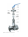
This master’s dissertation is conducted in cooperation with Fluoroseal Valves Inc., a
Canadian company whose headquarters are situated in Montréal. The company manufactures
industrial valves with inlet sizes that range from ½” to 24” (12.5 mm to 610 mm). PTFE is the
dominating material used to seal the fluid both internally and to the atmosphere. Internal
sealing is provided by the PTFE sleeve which is compressed between the body and the plug,
cf. Figure 1.1, while external sealing is guaranteed by the PTFE top seal. The most demanding
loading situation is found in the 24” valves when closed, and this master’s dissertation will
focus on this situation.
5
Figure 1.1. An explode view of a Fluoroseal plug valve.
6
1.2
Objective
The objective of this master’s dissertation is to study the stresses that act on the PTFE sleeve
in the 24” valve when blocked. This knowledge is sought in order to predict leakage and to
develop valves with higher classification. The implementation of the problem in a finite
element code is described in detail, and special attention is given to the non-linear stress-strain
relationship of PTFE, the viscoelastic behavior of PTFE and the contact interaction between
the parts.
1.3
Methodology
The work is divided into several steps:
•
•
•
•
•
1.4
Literature study of the properties of PTFE and review of constitutive
models suitable for modeling PTFE.
Documentation of the loading situation.
Constitutive modeling of PTFE.
Implementation of a pertinent finite element model in ABAQUS/Explicit
and ABAQUS/Standard.
Post processing and review of the results.
Disposition
This report describes the solution steps of the problem and it is divided into the following
sections:
•
•
•
•
•
In Chapter 2 the plug valve is presented. The reference case, obtained
from measurements is specified, which will be used during the finite
element model implementation and when reviewing the results.
Chapter 3 describes the mechanical properties of PTFE and presents the
constitutive modeling of the material.
Chapter 4 treats the implementation of the problem in detail.
Chapter 5 reviews the results obtained from the analysis and provides a
discussion of the solution.
Finally, a summary and suggestions of further work concludes the report
in Chapter 6.
All code produced throughout the project is documented in appendices at the end of the
report.
7
Chapter 2
Plug Valve
A plug valve can be used in any pipe system where control of the flow is of importance. The
plug lets the fluid pass as it is positioned inline with the fluid gate. As the plug is rotated 90
degrees, it blocks the valve and the fluid cannot come through. Fluoroseal Valves Inc. also
provides valves where the plugs allow intermediate states and control of the amount of flow.
There are also valves with three-way connections that can direct the flow in a T-junction of a
pipe system.
In this report, only the two-way 24” plug valve will be studied, as it is the one most exposed
to leakage. Its inlet measures 24” (610 mm) and it should withstand a fluid pressure of 675 psi
(4.65 MPa). When the pressure is applied, the valve has to be properly sealed in order not to
leak. The PTFE sleeve provides sealing, and its sealing capacity relies on the assembling
process. The assembling of the 24” valves has to be done manually by two assemblers and
with hydraulic presses. First, the PTFE sleeve is slowly inserted into the cast iron valve body
(cf. Figure 1.1). To prevent damage on the sleeve, a careful handling and a slow insertion is
important. Secondly, the steel plug is carefully inserted. This implies that the ribs in the cast
iron body compress the outer surface of the PTFE sleeve and the steel plug compresses the
entire inner surface of the sleeve (cf. Figure 1.1). These two steps can be seen as a forming of
the PTFE sleeve, and they require a great amount of time to let the PTFE relax into its new
shape. After these steps, the rest of the components, such as the top seal, the cover and the
rotation mechanism can be mounted, and the valve is ready to ship.
Fluoroseal Valves Inc. performs tests
on all 24” valves prior to shipping.
The valve is blocked and filled with
compressed air with a pressure of
675
psi
(4.65
MPa).
The
displacement of the plug is measured
and after 90 seconds the plug has
moved 1.5 mm. A small amount of
leakage occurs, and the leakage sites
are situated at the upper corners of
the outlet, cf. Figure 2.1.
In the present situation, the amount
of leakage is close to the maximum
allowed
and
therefore,
this
measurement will be used as
reference case in the calculations.
Figure 2.1. Leakage site upon testing of the valve.
8
Chapter 3
Material Properties
3.1
General Properties of PTFE
PTFE is a polymer discovered in 1938 by Roy Plunkett of the DuPont Company. Its chemical
structure consists of chains of carbon atoms bonded together, with branches of fluorine atoms
attached [3]. The material is often referred to as polytetrafluoroethylene (PTFE), while Teflon
is a registered trademark of the DuPont Company. Throughout this thesis, the name PTFE
will be used to label the material.
PTFE has become an important engineering material. Its major benefits are its non-adhesive
character, inertness, resistance to chemical attacks and relatively high strength. Moreover,
specific physical properties can be enhanced by adding filler compounds or altering the
manufacturing process. Some physical disadvantages that PTFE experiences are high
sensitivity to temperature changes and poor resistance to creep and stress relaxation. The
complex and highly non-linear nature of these characteristics presents a delicate task for any
engineer who wishes to predict the behavior of PTFE.
Another drawback that PTFE suffers from is its high melt viscosity that makes injection and
blow molding impossible, leaving more expensive manufacturing methods, such as sintering
and extrusion, the only choices for part production [7].
3.2
Microscopical Structure
The smallest component of any polymer is called the monomer. In PTFE, the monomer
consists of two carbon atoms, each of them having two fluorine atoms attached, cf. Figure 3.1.
When this unit is repeated a long chain is formed and thousands of such chains form the
macroscopical structure. Depending on the temperature and the manufacturing method, the
chains can exist in an ordered, aligned pattern, known as a crystalline state, or being entangled
with a random chain orientation, like cooked spaghetti in a bowl, known as an amorphous
state. In fact, both crystalline regions and amorphous regions may exist simultaneously, which
is the case in PTFE, which is referred to as a semi crystalline state.
Figure 3.1. The monomer of PTFE.
9
The bonds within each chain are strong covalent bonds. The secondary bonds that act between
two chains are weaker than the covalent bonds, and the larger the distance between two
chains, the weaker the secondary bond. In a crystalline region the chains are tightly packed
and consequently, the secondary bonds are stronger than in an amorphous region. The degree
of crystallization will therefore affect the strength of the polymer.
By adding energy, e.g. by rising the temperature, the distance between the chains will increase
and hence, the material will soften. Similarly, the distance between two chains will increase
upon stretching the material. However, the chains in the stretched material will slide with
time, causing the applied stress to decrease. This phenomenon is known as stress relaxation
and is due to the viscoelastic behavior of polymers. Stress relaxation is one of the major
causes for leakage in the valve studied and will be treated in detail later in this report.
One property that often is of importance for polymers is the glass transition temperature,
which is associated with the long-range molecular motions. Below the glass transition
temperature the molecules are restricted in motion and consequently very stiff, like a glass.
When the temperature is increased above the glass transition temperature a phase transition
occurs. Adjacent atoms might move as a unit, which results in a more flexible, leathery
structure. Since PTFE is a semi-crystalline polymer this behavior is less emphasized than in a
pure amorphous material. The glass transition temperature of PTFE is -97°C [2]. In this
application the temperature will be kept well over this value.
The flexibility will increase with increased temperature and when the melting temperature is
reached, the crystalline bonds are broken apart. By that time, the amorphous regions are
already in a liquid state, and the polymer enters a liquid. Differences in chain length and
between regions within the polymer make it difficult to define an absolute melting
temperature. It is rather defined as a temperature range, and for PTFE it is typically 328°C341°C [7].
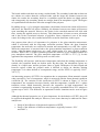
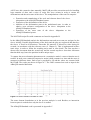
An interesting property of PTFE is its expansion due to temperature. Most materials expand
when exposed to a rise of temperature, which is measured with the linear thermal expansion
coefficient [4]. The variation of this coefficient for PTFE is shown in Figure 3.2. At low
temperatures, the expansion increases linearly with the temperature. Around 20°C, a phase
transition occurs, which drastically increases the expansion. At high temperatures, the
variation is exponentially increasing. The valve is typically assembled below 20°C whereas it
operates up to 200°C. The difference in expansion for those situations can be seen in Figure
3.2.
Although the thermal properties are of great importance for the behavior of PTFE, they will
be neglected throughout this analysis. However, some issues that may be addressed in future
analyses are:
•
•
Study of the influence of the thermal expansion of PTFE.
Study of the influence of different temperatures (typically between -50°C
and 200°C).
10
Figure 3.2. The variation of the linear thermal expansion coefficient with temperature [4].
3.3
Constitutive Modeling of PTFE
A constitutive model is a mathematical description of a material. It aims at relating physical
phenomenons such as stresses, strains, temperature and time to each other. The most known
constitutive model is Hooke’s law from 1676 which relates stress and strain linearly. It is
valid for metals subjected to moderate loading, but is less accurate for polymers, exhibiting
non-linearities at very low loading levels. In the 19th and 20th centuries much progress has
been done to develop the non-linear theory of materials by e.g. von Mises, Drucker and
Prager. In recent years, advanced constitutive models, that take the microscopical structure of
PTFE into account, have been developed. This was done by, for instance Bergström and
Hilbert [2]. These constitutive models are more accurate than the ones available in general
finite element softwares like ABAQUS, but they are only commercially available and the
implementation of such a model is not possible within the time frame of a master’s thesis.
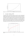
Figure 3.3. Stress-strain relationship for PTFE in compression at room temperature and a strain rate
-4 -1
of 10 s .
11
The stress-strain relationship for a uniaxially compressed PTFE specimen is shown in Figure
3.3. This behavior is not similar to the ones expressed by the hyperelastic constitutive models,
which often are used for rubber and other polymers. It rather looks like a typical plasticity
model, e.g. the von Mises plasticity model [6]. Since the sleeve undergoes plastic deformation
(i.e. non-recoverable deformation) during assemblage, such a model appears to be valid, as
opposed to the hyperelastic models, in which the deformation is recovered upon unloading.
For a thorough presentation of the theory, reference is made to [6].
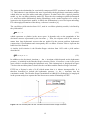
The von Mises yield criterion from 1913, used in von Mises plasticity models, is defined by
the yield surface
3J 2 − σ y 0 = 0
(3.1)
which represents a cylinder in the stress space. It depends only on the magnitude of the
deviatoric stresses represented by the invariant J 2 . Thus, the response will be the same no
matter how large hydrostatic stresses that are applied. In the present problem, hydrostatic
compression is predominant and consequently the von Mises criterion fails to represent the
behavior of the material.
A similar yield criterion is the Drucker-Prager criterion from 1952 with a yield surface
described as
3 J 2 + I1 tan β − d = 0
(3.2)
In addition to the deviatoric invariant J 2 , the I1 invariant, which depends on the hydrostatic
pressure, is included in the Drucker-Prager criterion. Hence, it becomes a cone in the stress
space which is confined along the hydrostatic axis. This characteristic is displayed in Figure
3.4 where the meridian plane is shown for the von Mises and the Drucker-Prager criterions.
PTFE has a Poisson’s ratio of 0.45 which means that it is almost incompressible. It is
therefore beneficial to include the hydrostatic pressure, i.e. the I1 invariant, into the
constitutive model. The Drucker-Prager formulation in ABAQUS will therefore be employed
in the present analysis to capture the non-linear stress-strain relationship of PTFE.
Figure 3.4. The meridian plane for the von Mises and the Drucker-Prager criterions.
12
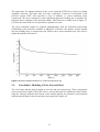
The main cause for leakage initiation in the valve is that the PTFE sleeve looses its sealing
capability with time. The stress state over time is therefore of interest. As described in the
previous section, PTFE will experience a loss of stiffness, i.e. stress relaxation, when
compressed. The stress relaxation is most significant right after loading, but it continues for
long time due to slipping of the molecular chains. This behavior is readily seen in Figure 3.5
[2] where the stress state in a test specimen is plotted over time.
The stress relaxation cannot be captured simultaneously with the non-linear stress-strain
relationship by the materials available in ABAQUS. Therefore, the analysis will be divided
into two loading steps; a compression step followed by a stress-relaxation step. This will be
further described in Section 4.2.
Figure 3.5. Stress relaxation behavior for a PTFE test specimen [2].
3.4
Constitutive Modeling of Cast Iron and Steel
The valve body and the plug are made of cast iron and steel respectively. These components
are not as heavily loaded as the PTFE sleeve, and can therefore be modeled as linear elastic.
Only the Young’s modulus, the Poisson’s ratio and the density are needed for each material
and the material data of cast iron and steel is presented in Chapter 4.5.
13
Chapter 4
Finite Element Model
This section will deal with the implementation of the present problem in the finite element
software ABAQUS. Readers not familiar with the finite element method are advised to
consult an introductory textbook on the topic, see for instance [5], for a thorough exposition
of the theory.
4.1
Introduction to ABAQUS and Explicit Dynamics
ABAQUS is a multi-purpose software package widely used for finite element simulations. Its
strength lies in its powerful solvers, ABAQUS/Standard and ABAQUS/Explicit, capable of
handling very complex analyses, combined with the interactive interface ABAQUS/CAE,
developed for pre- and post-processing.
ABAQUS/Standard is a general implicit finite element solver developed to solve static and
dynamic linear and non-linear problems. A global stiffness matrix is assembled and the
solution is obtained by solving a set of dependent equations simultaneously. A Newton
iteration procedure, which is unconditionally stable, is employed for non-linear formulations
and the time increment is adjusted as the solution progresses in order to obtain a stable, yet
time efficient solution.
There are situations where ABAQUS/Standard encounters problems finding a converged
solution. In analyses where bodies are in contact or where the effect of inertia has to be taken
into account the algorithm is less efficient due to the simultaneous solving of the equation
system in every increment. Moreover, for large structures considerably big memory and disk
space is needed. In such situations it is advantageous to use the explicit solver provided by
ABAQUS/Explicit. In this algorithm an uncoupled mass matrix is constructed and the nodal
accelerations are computed independently. The accelerations are integrated through time with
a central difference rule to obtain the displacements.
By using sufficiently small time increments, a stable solution is guaranteed without having to
check for global equilibrium. At all times, the time increment has to be smaller than the time
required for half a dilatation wave to cross any of the elements. If this requirement is not
fulfilled, numerical instabilities may occur, leading to unbounded solutions.
The time increment depends on the shortest element length in the model, the material stiffness
and the density. ABAQUS/Explicit computes the time increment automatically, and it is
typically in the range of 10-6, which is considerably smaller than the time increments used in
ABAQUS/Standard. Thus, ABAQUS/Explicit performs a large amount of inexpensive
calculations to reach the solution whereas ABAQUS/Standard performs fewer but more
computationally expensive calculations.
14
The global equilibrium is not guaranteed in an explicit solver, and it is therefore important to
verify that the external energy (e.g. external forces and pressures) equals the internal energy
(e.g. material deformation and friction). Furthermore, since the problem at hand is of quasistatic nature (i.e. inertia should not affect the solution), high kinetic energies are unwanted.
Finally, energies associated with the numerical implementation (labeled “artificial energy”)
should be kept at a moderate level.
Since the problem at hand exhibits complex material behavior as well as interaction between
several bodies, both ABAQUS/Standard and ABAQUS/Explicit are used in order to reach an
accurate and efficient solution.
4.2
Analysis Steps
When modeling the assembling process it has to be divided into several steps. It turns out that
the interactions between the valve parts (cf. Section 4.6) make it difficult to solve the problem
with the ABAQUS/Standard solver. Complex interactions are more readily solved by the
explicit algorithm provided by ABAQUS/Explicit, which accordingly will be used when
assembling the valve. However, ABAQUS/Explicit does not allow time dependent
constitutive models. Hence, ABAQUS/Standard will be used to evaluate the stress relaxation
behavior of the sleeve. The flow chart of the implementation is as shown in Figure 4.1.
Figure 4.1. Flow chart of the analysis.
In the assembling process, the sleeve is slowly pressed into the body. Since PTFE is highly
viscoelastic, it is important to insert the sleeve slowly to let the material relax and prevent
formation of cracks. The assembling process therefore lasts for approximately an hour. In this
analysis, it is assumed that the stress relaxation will take place after the assemblage and the
pressure application. This abstraction is necessary since only the built in material models will
be used.
The assemblage and the pressure application are modeled in ABAQUS/Explicit. To cut the
solving time, a much shorter time must be used in the analysis. It is found that a step time of
0.2 seconds yields efficient, yet accurate results, with small kinetic energy.
15
The plug is pressed into the sleeve from above, as seen in Figure 1. This means that the plug
and the sleeve slide over a long distance; a situation that causes problems in finite element
analysis. The large deformation of the sleeve and the fact that PTFE is almost incompressible
makes the situation further complicated. The plug will therefore be assembled radially, which
will be further described in section 4.3.
A fluid pressure corresponding to 1.5 mm movement of the plug will be applied. This will
cause further deformation of the sleeve. When the fluid pressure has been applied the PTFE is
allowed to relax. The stress and strain state of the sleeve is extracted from the
ABAQUS/Explicit analysis using MATLAB, and loaded into ABAQUS/Standard, where the
stresses and strains are applied, and a stress relaxation analysis is performed.
All code produced throughout this master thesis is presented in Appendices A, B and C. The
following sections describe its content.
4.3
Geometry of the Valve
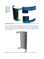
The valve studied in this thesis consists of several parts as shown in Figure 1.1. The parts are
read from Pro/Engineer and converted to AGIS format, which is imported in ABAQUS/CAE.
The parts that most severely are exposed to loading are the cast iron body, the PTFE sleeve
and the steel plug. These are the parts included in the finite element model, cf. Figure 4.2.
Due to symmetry of the valve, only half of the valve needs to be studied.
Figure 4.2. The geometry used in the finite element model. The plug is cut into two halves, labeled
“Plus” and “Minus”, in order to facilitate the assemblage.
16
The inner wall of the body is lined with ribs next to the inlet and outlet, which can be seen in
Figure 1.1 and Figure 4.3. The ribs help compress the sleeve in order to end up with a tight
seal as described in Chapter 2. It is therefore important to represent this geometry correctly,
but other parts of the geometry are slightly simplified in their representation in order to end up
with a proper mesh.
ribs
plug
sleeve
sleeve
body
expansion
Figure 4.3. The parts in the analysis in an exploded view.
When modeling the assembling of the plug it turns out that an abstraction has to be done. The
complex interactions between the parts make it impossible to insert the plug axially (i.e. insert
it from above, as in Figure 1.1). Instead, the plug is inserted radially, which can be seen as an
expansion of the plug. Thus, the plug is cut into two pieces (called “Plus” and “Minus”)
which initially overlap slightly (shown in black in Figure 4.2). The two pieces are displaced
radially until they reach their assembled positions.
4.4
Elements and Mesh
A solid brick element, C3D8R is chosen to represent the parts. It is a linear eight node
element with reduced integration [1] which is commonly used when representing solids. The
resulting mesh consists of 213 920 elements.
Reduced integration of an eight node element implies that the element is evaluated in only one
point, the centroid, providing a faster solution. However, certain deformation modes, so called
zero energy modes, may arise when using reduced integration which destroys the solution. To
overcome this difficulty, hourglass control is employed, cf. [1].
Further numerical control of the element is employed, namely distortion control and second
order accuracy. Interested readers should consult [1] for further details on the topic.
In explicit dynamics, the size of the smallest element is crucial for the increment used by the
solver. One small element may destroy the stability limit of the whole model, and therefore
mass scaling is used. Mass scaling implies that some small elements are assigned more mass.
This does not affect the total mass significantly, but has great influence on the solution time.
17
4.5
Material
The materials present in the model are cast iron, steel and PTFE. They are all assumed to
respond linearly to moderate loading, and their linear properties are listed in Table 4.1.
Material
Part
Density
Young’s Modulus
3
Cast Iron
Body
7200 kg/m
185 GPa
3
Steel
Plug
7800 kg/m
211 GPa
3
PTFE
Sleeve
2160 kg/m
482 MPa
Table 4.1. Density and elastic properties of the materials.
Poisson’s Ratio
0.3
0.3
0.45
The complicated microscopical structure of PTFE described in the Section 3.2 is more
complex than for steel and cast iron, and it is hard to incorporate in a mathematical model. In
recent years accurate models have been developed but they are expensive to purchase at
present. Of the material models implemented in ABAQUS it turns out that the Drucker-Prager
plasticity model is most suitable for modeling the constitutive behavior of PTFE.
In order to determine the parameters in the Drucker-Prager model, material testing needs to be
performed. A number of test results are available from the manufacturer and from academic
papers [2] and [7]. Since accurate material tests require high precision equipment the test data
gathered from these sources will be used throughout this thesis.
In [7], an investigation of the response of PTFE in compression for two different compounds
is presented. It was found that the loading rate and the temperature influence the response
significantly. The uniaxial behavior in compression, which is used to calibrate the DruckerPrager model, is obtained from test data for Teflon 7C at a loading rate of 10-4 strain/s at room
temperature [7]. Teflon 7C is a common PTFE compound very similar to the one used in the
sleeve. The data is presented as a graph, and to extract the values of stress and strain from the
graph, a code is written in MATLAB which extracts the points on the curve needed to define
the plastic behavior. The data, shown in Figure 3.3, is fit to the Drucker-Prager model,
described in equation 3.2 according to the following method.
The stress tensor obtained from the test data is expressed by
σ 0 0 
σ ij =  0 0 0 
 0
(4.1)
0 0 
where σ is negative for uniaxial compression. It should be fit to
t − p tan β − d = 0
(4.2)
in accordance with [1]. In (4.2) p and t are, for uniaxial compression
1
1
p = − σ ii = − σ
3
3
(4.3)
t=σ
(4.4)
and
18
With these manipulations, (4.2) becomes
1
t − p tan β − d = σ + σ tan β − d = 0
3
(4.5)
A plot of the test data (shown in green) and the curve (shown in black) are presented in Figure
4.4 and the parameters obtained from the curve fitting are summarized in Table 4.2. The K
value is a measurement of the ratio of the flow stress in triaxial tension to the flow stress in
triaxial compression and it is typically set to 1 [1].
Parameter
K
Value
1
β
1.25
0
d
Table 4.2. Parameters used in the Drucker-Prager model.
Figure 4.4. Curve fitting of test data to the Drucker-Prager constitutive model.
19
4.6
Interactions and Boundary Conditions
The problem at hand includes contact where the interaction of bodies will be the major cause
of deformation. In a contact analysis, several meshes interact, resulting in discontinuities over
the interaction boundary. This in turn put high demands on the solver.
Since ABAQUS/Explicit handles interactions in a simpler fashion than ABAQUS/Standard, it
will be used for all contact analyses. ABAQUS/Explicit provides two interaction
formulations: general contact and contact pairs. The latter one is used throughout this
analysis.
In a contact pair, one surface is the master surface and the other is the slave surface. The
nodes on a master surface are allowed to penetrate the element sides on a slave surface. In
general, the surface with higher Young’s modulus should act as a master surface, and
consequently, the body and the plug are master surfaces in both contact pairs (cf. Table 4.3)
Contact Pair
Master Surface
Slave Surface
1
Body
Sleeve
2
Plug
Sleeve
Table 4.3. Contact pairs while assembling the valve.
Boundary conditions are prescribed in order to:
• model the ground on which the valve stands.
• displace the sleeve and the plug parts during assembling.
• apply the fluid pressure during loading
• clamp the model in the symmetry plane.
A summary of all boundary conditions assigned to the parts are presented in Table 4.4 and the
displacements of the parts are shown in Figure 4.5.
Body
Plug Plus
Plug Minus
Sleeve
Assembling of the Sleeve
Assembling of the Plug
Fluid Pressure Application
- bottom surface: confined in x and y
- symmetry plane: confined in z
- cut surface: confined in x
- bottom surface: confined in y
- symmetry plane: confined in z
- cut surface: confined in x
- bottom surface: confined in y
- symmetry plane: confined in z
- one node: confined in x
- top surface: displacement in y
- symmetry plane: confined in z
no changes
no changes
- cut surface: displacement in x
- cut surface: displacement in x
- symmetry plane: displacement in z
- cut surface: displacement in x
- cut surface: displacement in x
- symmetry plane: displacement in z
no changes
no changes
Table 4.4. Summary of all boundary conditions assigned to the parts throughout the analysis.
20
Figure 4.5. Displacements of the parts by assigning non-zero boundary conditions.
The displacements are applied in a smooth manner in order to avoid sudden jumps in
acceleration. This is of great importance since the displacements are obtained through
integration of the accelerations in explicit dynamics. The amplitude curve shown in Figure 4.6
is suitable for quasi static analyses since it ensures a smooth acceleration.
Figure 4.6. Amplitude curve used for the displacements of the parts.
4.7
Stress Relaxation
After the valve has been assembled interest is directed towards the stress relaxation of the
sleeve. The resulting stress state of the sleeve is printed to a text file at the end of the
ABAQUS/Explicit analysis. However, this text file needs to be formatted in order to use the
data in an ABAQUS/Standard analysis and due to the size of the file, 132 megabytes of
21
ASCII text, this cannot be done manually. MATLAB provides convenient tools for handling
large amounts of data, and a series of script files were written in order to extract the
deformations and the stress state of the sleeve. The manipulations of the text file comprise:
•
•
•
•
Extraction and renumbering of the node and element data of the sleeve.
Adaptation to the ABAQUS/Standard syntax.
Extraction of the deformation of the sleeve.
Addition of the deformation state to the undeformed state, in order to
obtain a new reference configuration of the sleeve. Adaptation to the
ABAQUS/Standard syntax.
Extraction of the stress state of the sleeve. Adaptation to the
ABAQUS/Standard syntax.
The MATLAB script files with comments are found in Appendix B.
In the ABAQUS/Standard analysis the deformation state and stress state are assigned to the
sleeve initially. Possible displacements of the body and the plug are neglected and therefore
the sleeve is fixed in all directions. Thereafter the material is allowed to relax during 90
seconds, in accordance with the reference case (cf. Chapter 2). This is implemented in three
static steps, in order to follow the resulting stress state in close detail. The first step has a
shorter time increment than the second step and the second step has a short time increment
than the third step, hence the partition in three unique steps.
To capture the stress relaxation phenomenon in a constitutive model, a stress relaxation test is
needed. In such a test a uniaxial compressive strain is held constant over time and the stress is
measured at different times. Such a test is provided by [4] and the values are extracted with
MATLAB. The results are shown in Figure 4.7. The values extracted are used as input in the
ABAQUS material definition.
Figure 4.7. Stress relaxation test data for PTFE.
The same element formulation as in the previous analysis is used. Besides, no interaction
between parts is needed since only the sleeve is studied.
The ABAQUS/Standard code is presented in Appendix C.
22
Chapter 5
Results
In this section the results from the analysis are presented and discussed. Since Fluoroseal
Valves Inc. has not performed any calculations prior to the present one, it is impossible to
validate the calculations. The purpose of this work is rather to form a basis for future
calculations where refinements in the material model and parametric studies may be
performed in accordance with measured data. Consequently, all graphs, material data,
MATLAB and ABAQUS code are documented by Fluoroseal Valves for future use.
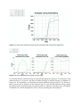
5.1
Energy Balance
As described in Section 4.1, it is in an explicit dynamics analysis important to study the
energies present in the model. The external energy should be balanced by the internal energy
in order to guarantee an accurate solution. Figure 5.1 displays the energy plot during the three
steps performed in ABAQUS/Explicit and Table 5.1 explains the meaning of the different
energies. Figure 5.2a-c displays the energies for each step in detail.
Label
Energy
Description
ALLAE
artificial energy
energy due to hourglass control of partly integrated elements
ALLWK
external work
energy supplied by external forces and prescribed displacements
ALLFD
frictional dissipation energy lost during contact between parts by friction
ALLIE
internal energy
energy stored by the material, i.e. internal forces
ALLSE
elastic strain energy elastic (i.e. recoverable) deformation
ALLPD
plastic dissipation
plastic (i.e. non-recoverable) deformation
ALLKE
kinetic energy
energy used to move parts
ALLVD
viscous dissipation
energy due to viscous materials or numerical controls
Table 5.1. Energies associated with the model.
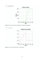
It is seen that not much deformation takes place in the first step. The main part of the external
energy is used to translate the sleeve downwards, where it slides against the body and deforms
slightly. The artificial and viscous energies are close to zero during the entire step.
During the assembling of the plug a great deal of deformation takes place, as seen in
Figure 5.2b. Initially, the plug parts and the sleeve are not in contact and the external work is
balanced by the energy used to move the plug parts. As the parts start to interact the internal
energy dominates the energy plot as the sleeve deforms. The internal energy consists of a
recoverable and a non-recoverable part (ALLSE and ALLPD), as indicated in Table 5.1 and
their distribution are shown in Figure 5.3. Obviously, the main part of the deformation is nonrecoverable, and associated with the non-linear characteristic of PTFE. The internal energy
continues to rise as the fluid pressure is applied since the sleeve is put under heavy
compression, cf. Figure 5.2c.
23
Figure 5.1. Internal and external energies during assembling and fluid pressure application.
Figure 5.2. Internal and external energies for each step.
It is desired that the artificial energy is kept low throughout the analysis. To determine if the
artificial energy is excessive, the ratio of artificial energy to internal energy is evaluated, cf.
Figure 5.4. As a guideline, it is desirable to keep the artificial energy below 5% [1]. However,
this is not the case at all times in this analysis, but it is seen that the artificial energy during
the fluid pressure application does not pass beyond 6%, which is considered to be acceptable.
In addition, the viscous dissipation is more or less zero during the entire analysis.
24
Figure 5.3. Internal energy during assembling and fluid pressure application.
Figure 5.4. The ratio of artificial energy to internal energy.
25
5.2
Stress and Strain Analysis
The objective of this work is to find the stress distribution in the PTFE sleeve with viscosity
taken into account. In order to use the general ABAQUS element library all loading is
assumed to take place prior to stress relaxation of PTFE. After the loading phase, the sleeve is
considered linear elastic-viscoelastic, and the stress relaxation is studied. This is of course an
abstraction, but is necessary in order to use the adapted analysis method.
The assembling process and the fluid pressure application give rise to an inhomogeneous
stress field in the sleeve. The leakage is initiated due to this inhomogeneous stress field since
the capability of the sleeve to resist the pressure varies with position. A stress plot of the
sleeve after the fluid pressure application, before any stress relaxation has taken place, is
shown in Figure 5.5a-b. The highest stresses are found in the marked areas, as are the highest
plastic strains, cf. Figure 5.6. Since the plastic strains are non-recoverable, the deformation
caused by them would stay if the valve were disassembled. Similarly, the plastic deformations
remain when PTFE relaxes and as the stress decreases, the sleeve looses its capacity to resist
the fluid pressure and leakage occurs.
a)
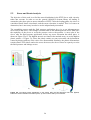
b)
Figure 5.5. Von Mises stress distribution in the sleeve after the fluid pressure has been applied,
before the stress relaxation has taken place, a) outer surface and b) inner surface.
26
Figure 5.6. Plastic strains in the sleeve after the fluid pressure has been applied, before the stress
relaxation has taken place.
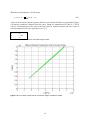
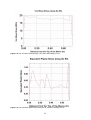
Figure 5.8 displays the von Mises stress along the most severely loaded path of the sleeve (cf.
Figure 5.7). The plastic strains are displayed in Figure 5.9. Excessive stresses and plastic
strains are observed close to the top and bottom of the inlet, which is in close agreement with
the actual leakage sites (cf. Figure 2.1). The von Mises stress peaks at 19.8 MPa close to the
upper corner of the inlet.
Figure 5.7. The path, corresponding to the rib, along which the stresses and strains are plotted.
27
Figure 5.8. The von Mises stress along the rib, where the leakage occurs.
Figure 5.9. The equivalent plastic strain along the rib, where the leakage occurs.
28
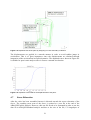
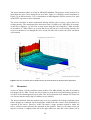
The stress relaxation phase is solved in ABAQUS/Standard. The purpose of this analysis is to
study how the stress varies along the rib over time. Figure 5.10 displays several snapshots of
Figure 5.8 at different times. It is a visualization of what happens with the stresses over time
as the PTFE experience stress relaxation.
The stress relaxation is much emphasized initially and the sleeve looses a great deal of its
sealing capacity. The maximum stress decreases from 19.8 MPa to 8.1 MPa after 90 seconds,
as the sleeve displaces 1.5 mm. The average stress along the rib is initially 17 MPa and after
90 seconds it is 7 MPa. Hence, in average the sleeve has lost 60 % of its sealing capacity due
to stress relaxation. Even though the curve seams flat after 90 seconds, the stress relaxation
will continue.
Figure 5.10. The von Mises stress variation during 90 seconds after the fluid pressure application.
5.3
Discussion
As seen in Figure 5.10 the von Mises stress peaks at 19.8 MPa initially, but after 90 seconds it
has dropped to 8.1 MPa. Clearly, the sleeve looses a great deal of its load bearing capacity as
an effect of the inhomogeneous stress state. The stress relaxation will continue for hours, but
it is obvious that the major drop of stiffness occurs initially.
The stresses obtained from this analysis may serve as a guideline for leakage prediction when
future designs are evaluated. By increasing the width of the ribs a better stress distribution is
expected in the sleeve. However, wider ribs imply a larger moment needed to rotate the
sleeve, which in turns increases the demands on the gearbox. However, the shape of the rib
may be reviewed. A slightly wider rib in the upper and lower part and a more narrow rib in
29
the midst of the rib would produce a different result that could be beneficial from a leakage
point of view. By assigning a larger area where stresses are high, a more uniform stress
distribution is expected than the one shown in Figure 5.8. However, design evaluations and
calculations have to be performed before any conclusions can be drawn.
In addition, different compounds of the PTFE may be used in certain applications, which may
have a better resistance to stress relaxation. In general, by adding filler compounds the effect
of stress relaxation decreases. Besides the mechanical properties, other properties such as
inertness and temperature resistance need to be taken into account before a change of material
can be done.
Finally, a modification of the assembling method with use of more lubricants that decrease the
friction forces between the parts would most likely decrease the stresses.
30
Chapter 6
Conclusions
6.1 Achievements
An analysis method that enables evaluation of the response of PTFE has been developed. By
means of the standard ABAQUS code it captures the behavior of the sleeve in principal. The
input data used in the analysis are the geometries obtained from the Pro/Engineer models and
material data. The model is applicable to other valves as well, by providing the corresponding
geometry as input data. Also, different compounds of PTFE may be evaluated after some
calibration of the material model. Development of the valve and construction of new designs
may be verified with this model prior to manufacturing it, in order to avoid excessive stresses.
Also, parametric studies may be performed to optimize the performance of the sealing
capability of the sleeve.
6.2 Future Work
Due to lack of proper measurements the model might need to be calibrated and modified
slightly. Calibration includes choice of material model, the parameters in the material model,
the coefficient of friction, the model damping, and numerical controls of the elements.
Furthermore, the loading case and the effect of mesh refinements could be investigated.
One issue that has not been addressed in this work is the influence of temperature, which
might be of importance in certain applications. There is data available in i.e. [4] and a study of
the effect at elevated temperatures and corresponding phase transitions could easily be
performed.
In the long run, if very precise predictions of the sleeve response are needed, a development
of an advanced constitutive model may be considered. The theory of such a model is available
in [2], and with advanced knowledge in ABAQUS programming and solid mechanics it could
be implemented. However, if this option is considered, it is important to keep in mind that an
advanced material model requires accurate material data and precise measurements. Hence, a
great deal of measuring and research has to run parallel with the model development.
31
Bibliography
[1]
ABAQUS Version 6.5 Documentation. ABAQUS Analysis User’s Manual, ABAQUS
Inc, 2004.
[2]
Bergström, J.S, Hilbert Jr, L.B., A Constitutive Model for Predicting the Large
Deformation Thermomechanical Behavior of Fluoropolymers, Mechanics of Materials
37, 2005, pages 899-913.
[3]
Brent Strong, A., Plastics, Materials and Processing, Third Edition, 2006, Prentice
Hall.
[4]
DuPont Fluoroproducts, DuPontTM Teflon® PTFE Properties Handbook, Edition
220313.
[5]
Ottosen, N., Petersson, H., Introduction to the Finite Element Method, First Edition,
1992, Prentice Hall.
[6]
Ottosen, N., Ristinmaa, M., The Mechanics of Constitutive Modelling, Volume 1,
1999, Lund University.
[7]
Rae, P.J., Dattelbaum, D.M., The Properties of Poly(tetrafluoroethylene) (PTFE) in
Compression, Polymer 45, 2004, pages 7615-7625.
32
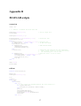
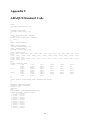
Appendix A
ABAQUS/Explicit Code
*Heading
** Job name: half1 Model name: Model-1
*Preprint, echo=NO, model=NO, history=NO, contact=NO
**
** PARTS
**
** The .inp-files contain *NODE, *ELEMENT, *NSET, *ELSET and *SOLID SECTION
*Include, input=m_body.inp
*Include, input=m_plugminus.inp
*Include, input=m_plugplus.inp
*Include, input=m_sleeve.inp
**
**
** ASSEMBLY
**
*Assembly, name=Assembly
**
*Instance, name=BodyAssem, part=Body
*End Instance
**
*Instance, name=PlugMinusAssem, part=PlugMinus
0.007,
0.,
-0.007
*End Instance
**
*Instance, name=PlugPlusAssem, part=PlugPlus
-0.007,
0.,
-0.007
*End Instance
**
*Instance, name=SleeveAssem, part=Sleeve
0.,
0.07,
0.
*End Instance
**
*Include, input=m_nodeselements.inp
*End Assembly
**
** ELEMENT CONTROLS
**
*Section Controls, name=EC-1, DISTORTION CONTROL=YES, hourglass=ENHANCED,
accuracy=YES
1., 1., 1.
*Amplitude, name=Amp-1, definition=SMOOTH STEP
0., 0., 0.2, 1.
**
** MATERIALS
**
*Material, name=PtfeDp
*Density
2160.,
*Drucker Prager
1.25, 1.0
*Drucker Prager Hardening
*Include, input=m_DP_param.inp
*Elastic
4.82e+08, 0.45
*Material, name=Steel
*Density
7800.,
*Elastic
2.11e+11, 0.3
*Material, name=CastIron
*Density
7200.,
*Elastic
1.85e+11, 0.3
33
second
order
**
** INTERACTION PROPERTIES
**
*Surface Interaction, name=Friction
*Friction
0.1,
**
** BOUNDARY CONDITIONS
**
** Name: BodyX Type: Displacement/Rotation
*Boundary
_PickedSet25, 1, 1
** Name: BodyY Type: Displacement/Rotation
*Boundary
_PickedSet28, 2, 2
** Name: BodyZ Type: Displacement/Rotation
*Boundary
_PickedSet32, 3, 3
** Name: PlugMinusX Type: Displacement/Rotation
*Boundary
_PickedSet36, 1, 1
** Name: PlugMinusY Type: Displacement/Rotation
*Boundary
_PickedSet29, 2, 2
** Name: PlugMinusZ Type: Displacement/Rotation
*Boundary
_PickedSet33, 3, 3
** Name: PlugPlusX Type: Displacement/Rotation
*Boundary
_PickedSet37, 1, 1
** Name: PlugPlusY Type: Displacement/Rotation
*Boundary
_PickedSet30, 2, 2
** Name: PlugPlusZ Type: Displacement/Rotation
*Boundary
_PickedSet34, 3, 3
** Name: SleeveX Type: Displacement/Rotation
*Boundary
_PickedSet24, 1, 1
** Name: SleeveY Type: Displacement/Rotation
*Boundary
_PickedSet31, 2, 2
** Name: SleeveZ Type: Displacement/Rotation
*Boundary
_PickedSet35, 3, 3
** ---------------------------------------------------------------**
** STEP: Sleeve
**
*Step, name=Sleeve
*Dynamic, Explicit
, 0.2
*Bulk Viscosity
0.06, 1.2
** Mass Scaling: Semi-Automatic
**
Whole Model
*Fixed Mass Scaling, dt=1e-05, type=below min
**
** BOUNDARY CONDITIONS
**
** Name: SleeveY Type: Displacement/Rotation
*Boundary, amplitude=Amp-1
_PickedSet31, 2, 2, -0.07
**
** INTERACTIONS
**
** Interaction: BodySleeve
*Contact Pair, interaction=Friction, mechanical constraint=PENALTY, cpset=BodySleeve
_PickedSurf18, _PickedSurf19
34
**
** OUTPUT REQUESTS
**
** FIELD OUTPUT: F-Output-1
**
*Output, field, variable=PRESELECT, number interval=1
**
** HISTORY OUTPUT: H-Output-1
**
*Output, history, time interval=0.02
*Energy Output
ALLAE, ALLFD, ALLIE, ALLKE, ALLPD, ALLSE, ALLVD, ALLWK, ETOTAL
*End Step
** ---------------------------------------------------------------**
** STEP: Plug
**
*Step, name=Plug
*Dynamic, Explicit
, 0.2
*Bulk Viscosity
0.06, 1.2
** Mass Scaling: Semi-Automatic
**
Whole Model
*Fixed Mass Scaling, dt=1e-05, type=below min
**
** BOUNDARY CONDITIONS
**
** Name: PlugMinusX Type: Displacement/Rotation
*Boundary, amplitude=Amp-1
_PickedSet36, 1, 1, -0.007
** Name: PlugMinusZ Type: Displacement/Rotation
*Boundary, amplitude=Amp-1
_PickedSet33, 3, 3, 0.007
** Name: PlugPlusX Type: Displacement/Rotation
*Boundary, amplitude=Amp-1
_PickedSet37, 1, 1, 0.007
** Name: PlugPlusZ Type: Displacement/Rotation
*Boundary, amplitude=Amp-1
_PickedSet34, 3, 3, 0.007
**
** INTERACTIONS
**
** Interaction: PlugMinusSleeve
*Contact Pair, interaction=Friction, mechanical constraint=PENALTY, cpset=PlugMinusSleeve
_PickedSurf20, _PickedSurf21
** Interaction: PlugPlus
*Contact Pair, interaction=Friction, mechanical constraint=PENALTY, cpset=PlugPlus
_PickedSurf22, _PickedSurf23
**
** OUTPUT REQUESTS
**
** FIELD OUTPUT: F-Output-1
**
*Output, field, variable=PRESELECT, number interval=1
**
** HISTORY OUTPUT: H-Output-1
**
*Output, history, time interval=0.02
*Energy Output
ALLAE, ALLFD, ALLIE, ALLKE, ALLPD, ALLSE, ALLVD, ALLWK, ETOTAL
*End Step
** ----------------------------------------------------------------
35
**
** STEP: SideLoad
**
*Step, name=SideLoad
*Dynamic, Explicit
, 0.2
*Bulk Viscosity
0.06, 1.2
** Mass Scaling: Semi-Automatic
**
Whole Model
*Fixed Mass Scaling, dt=1e-05, type=below min
**
** BOUNDARY CONDITIONS
**
** Name: PlugMinusX Type: Displacement/Rotation
*Boundary, amplitude=Amp-1
_PickedSet36, 1, 1, 0.0015
** Name: PlugPlusX Type: Displacement/Rotation
*Boundary, amplitude=Amp-1
_PickedSet37, 1, 1, 0.0015
**
** OUTPUT REQUESTS
**
*Restart, write, number interval=1, time marks=NO
**
** FIELD OUTPUT: F-Output-1
**
*Output, field, variable=PRESELECT, number interval=1
*NODE OUTPUT, NSET=NSLEEVE
U
*ELEMENT OUTPUT, ELSET=ESLEEVE
S
*FILE OUTPUT, NUMBER INTERVAL=1
*NODE FILE, NSET=NSLEEVE
U
*EL FILE, ELSET=ESLEEVE
S
**
** HISTORY OUTPUT: H-Output-1
**
*Output, history, time interval=0.02
*Energy Output
ALLAE, ALLFD, ALLIE, ALLKE, ALLPD, ALLSE, ALLVD, ALLWK, ETOTAL
*End Step
36
Appendix B
MATLAB scripts
extract1.m
clear, clc
% --- Extract a formated file from half.fin
fid=fopen('out.fin','w');
fclose(fid);
% Set up output file
fid=fopen('half.fin','r');
A=textscan(fid,'%s',1,'delimiter','\n');
C=char(A{1,1}(1,1)');
while 1
B=textscan(fid,'%s',1,'delimiter','\n');
if isempty(B{1})
break,
end;
D=char(B{1,1}(1,1)');
if length(D)<80
nblanks=80-length(D);
D=[blanks(nblanks) D];
end
C=tofile(C,D);
% Read first line
% Read new line
% If EOF then break
% Add removed blanks
% Subroutine that extracts all the characters
%
from C and D, writes to out.fin and returns
%
the remaining part of D as Cnew.
if length(C)<25
% Make sure that C is not to short
B=textscan(fid,'%s',1,'delimiter','\n');
if isempty(B{1})
break,
end;
D=char(B{1,1}(1,1)');
C=[C D];
end
end
disp('done')
fclose(fid);
tofile.m
function Cout=tofile(C,D)
TOT=[C D];
fid=fopen('out.fin','a');
i=0;
a=false;
while i<=80
i=i+1;
switch TOT(i)
case {'I'}
% --- If C and D are appended without the first blank of D
if ~isspace(TOT(i+1))
TOT=[TOT(1:i) blanks(1) TOT(i+1:end)];
end
pos=i+2;
len=str2num(TOT(pos));
val=TOT(1,pos+1:pos+len);
fprintf(fid,'%i,\t',str2num(val));
i=pos+len;
case {'D'}
37
% --- If C and D are appended without the first blank of D
if ~isspace(TOT(i+1)) & TOT(i+1)~='-'
TOT=[TOT(1:i) blanks(1) TOT(i+1:end)];
end
pos=i+1;
len=21;
if TOT(1,pos+len+1)~='I' | TOT(1,pos+len+1)~='D' | TOT(1,pos+len+1)~='E' ...
TOT(1,pos+len+1)~='A' | TOT(1,pos+len+1)~='*';
len=21;
end
val=TOT(1,pos:pos+len);
fprintf(fid,'%s,\t',val);
i=pos+len;
case {'E'}
% --- If C and D are appended without the first blank of D
if ~isspace(TOT(i+1)) & TOT(i+1)~='-'
TOT=[TOT(1:i) blanks(1) TOT(i+1:end)];
end
pos=i+1;
len=21;
if TOT(1,pos+len+1)~='I' | TOT(1,pos+len+1)~='D' | TOT(1,pos+len+1)~='E' ...
TOT(1,pos+len+1)~='A' | TOT(1,pos+len+1)~='*';
len=21;
end
val=TOT(1,pos:pos+len);
fprintf(fid,'%s,\t',val);
i=pos+len;
case {'A'}
pos=i+1;
len=7;
val=TOT(1,pos:pos+len);
fprintf(fid,'%s,\t',val);
i=pos+len;
case {'*'}
fprintf(fid,'\n');
end
end
fclose(fid);
Cout=TOT(i+1:end);
extract2.m
clear, clc
% --- Change from 0.00D+00 to 0.00E+00
fido=fopen('out2.fin','w');
fclose(fido);
% Set up output file
fid=fopen('disps.fin','r');
while 1
A=textscan(fid,'%s',1,'delimiter','\n');
if isempty(A{1})
break,
end;
C=char(A{1,1}(1,1)');
C(27)='E';
C(51)='E';
C(75)='E';
fido=fopen('out2.fin','a');
fprintf(fido,'%s,\n',C);
fclose(fido);
end
disp('done')
fclose(fid);
% Read first line
% If EOF then break
38
extract3.m
clear, clc
% --- Set local node numbers and sort the displacement data
fido=fopen('dispsort.fin','w');
fclose(fido);
% Set up output file
fid=fopen('disp.fin','r');
DISP=[];
while 1
A=textscan(fid,'%s',1,'delimiter','\n');
if isempty(A{1})
break,
end;
disp=str2num(char(A{1,1}(1,1)'));
DISP=[DISP;disp];
end
fclose(fid);
1
DISP(:,1)=DISP(:,1)-156528;
DISP=sortrows(DISP);
[len dum]=size(DISP);
% If EOF then break
fido=fopen('dispsort.fin','a');
for i=1:len
fprintf(fido,'%i,\t%15.6e,\t%15.6e,\t%15.6e\n',DISP(i,:));
end
fclose(fido);
extract4.m
clear, clc
% --- Set up the displacement data for the *BOUNDARY format
fido=fopen('sleeve_u.inp','w');
fclose(fido);
% Set up output file
fid=fopen('sleeve_u.fin','r');
fido=fopen('sleeve_u.inp','a');
while 1
A=textscan(fid,'%s',1,'delimiter','\n');
if isempty(A{1})
break,
end;
% If EOF then break
C=str2num(char(A{1,1}(1,1)'));
C=[C(1) 1 1 C(2) C(1) 2 2 C(3) C(1) 3 3 C(4)];
fprintf(fido,'%i,\t%i, %i,\t%15.6e\n%i,\t%i, %i,\t%15.6e\n%i,\t%i, %i,\t%15.6e\n',C);
end
fclose(fid);
fclose(fido);
disp('done')
extract5.m
clear, clc
% --- Add the displacements to the node coordinates for an updated configuration
fido=fopen('sleeve_n_updated.inp','w');
fclose(fido);
% Set up output file
fid1=fopen('sleeve_n.inp','r');
fid2=fopen('sleeve_u.fin','r');
fido=fopen('sleeve_n_updated.inp','a');
while 1
A=textscan(fid1,'%s',1,'delimiter','\n');
B=textscan(fid2,'%s',1,'delimiter','\n');
if isempty(A{1})
break,
end;
% If EOF then break
39
C=str2num(char(A{1,1}(1,1)'));
D=str2num(char(B{1,1}(1,1)'));
nnum=C(1);
coord=C(2:4);
disp=D(2:4);
newcoord=coord+disp;
fprintf(fido,'%i,\t%15.6e,\t%15.6e,\t%15.6e\n',[nnum newcoord]);
end
fclose(fid1);
fclose(fid2);
fclose(fido);
extract_stress1.m
clear, clc
% --- Set up the stresses for *INITIAL CONDITION
fido=fopen('stressout1.fin','w');
fclose(fido);
% Set up output file
fid=fopen('stress1.fin','r');
fido=fopen('stressout1.fin','a');
while 1
A=textscan(fid,'%s',1,'delimiter','\n');
if isempty(A{1})
break,
end;
% If EOF then break
C=(char(A{1,1}(1,1)'));
el=str2num(C(8:13));
stressID=str2num(C(4:5));
if el>100000
elnum=el;
elseif stressID==11
stress=str2num(C(8:end));
fprintf(fido,'%i,\t%15.6e,\t%15.6e,\t%15.6e,\t%15.6e,\t%15.6e,\t%15.6e\n',[elnum
stress]);
end
end
fclose(fid);
fclose(fido);
extract_stress2.m
clear, clc
% --- Set local element numbers and sort the stress data
fido=fopen('stressout2.fin','w');
fclose(fido);
% Set up output file
fid=fopen('stressout1.fin','r');
STRESS=[];
while 1
A=textscan(fid,'%s',1,'delimiter','\n');
if isempty(A{1})
break,
end;
stress=str2num(char(A{1,1}(1,1)'));
STRESS=[STRESS;stress];
end
fclose(fid);
1
STRESS(:,1)=STRESS(:,1)-135258;
STRESS=sortrows(STRESS);
[len dum]=size(STRESS);
% If EOF then break
fido=fopen('stressout2.fin','a');
for i=1:len
fprintf(fido,'%i,\t%15.6e,\t%15.6e,\t%15.6e,\t%15.6e,\t%15.6e,\t%15.6e\n',STRESS(i,:));
end
fclose(fido);
40
Appendix C
ABAQUS/Standard Code
*NODE
*INCLUDE, INPUT=sleeve_n.inp
**
**
*ELEMENT, TYPE=C3D8R
*INCLUDE, INPUT=sleeve_e.inp
**
**
*NSET, NSET=SLEEVE_NSET, GENERATE
1, 90918, 1
*ELSET, ELSET=SLEEVE_ELSET, GENERATE
1, 78662, 1
**
**
*NSET, NSET=BOUNDARY_X
21,
*NSET, NSET=BOUNDARY_Y
*INCLUDE, INPUT=sleeve_y.inp
*NSET, NSET=BOUNDARY_Z
*INCLUDE, INPUT=sleeve_z.inp
**
*NSET, NSET=RIB_NSET
1306, 10041, 9923, 9805, 9687, 9569, 9451, 9333, 9215, 9097, 424, 5012, 4894, 289, 16310,
16311,
16312, 16313, 16294, 16295, 16296, 16277, 16278, 16259, 16260, 16261, 16242, 16243, 16244,
16245, 16226, 16227,
16228, 16209, 1663, 21042, 21101, 21160, 21219, 21278, 21337, 21396, 21455, 21514, 21573,
22238, 22239, 22240,
2236
**
*ELSET, ELSET=RIB_ELSET
17990,
17871,
17752,
17633,
17514,
17395,
17276,
17157,
17038,
16919,
2740,
1788,
836,
42957,
42757,
42767,
42777,
42787,
42587,
42597,
42607,
42407,
42417,
42427,
42437,
42237,
42037,
42047,
42057,
42067,
41867,
41877,
41887,
41687,
54332,
54863,
55394,
55925,
56456,
56987,
57518,
58049,
58580,
59111,
66179,
66180,
66181,
66182,
**
**
*SOLID SECTION, ELSET=SLEEVE_ELSET, MATERIAL=PTFE_ELASTIC
1.,
**
**
*MATERIAL, NAME=PTFE_ELASTIC
*ELASTIC, MODULI=LONG TERM
4.82e+08, .45
*DENSITY
2160.
*VISCOELASTIC, TIME=RELAXATION TEST DATA
*SHEAR TEST DATA, SHRINF=0.409979
1., 0.001067
0.980599, 0.001386
0.971032, 0.00167
0.924608, 0.003118
0.897826, 0.004528
0.863317, 0.007284
0.838317, 0.010575
0.814023, 0.015071
0.790447, 0.020691
0.752652, 0.035201
0.723731, 0.063331
0.695908, 0.097242
41
0.669162, 0.14519
0.643445,
0.2402
0.618711, 0.39368
0.600791,
0.5405
0.583392, 0.77026
0.56649,
1.1501
0.550086,
1.4931
0.534145,
1.9934
0.523779,
2.9214
0.513622,
3.8282
0.50365,
5.1588
0.489062,
6.7602
0.479576,
8.4552
0.47489,
10.
0.461135,
11.609
0.456647,
15.071
0.452193,
17.991
0.447785,
19.566
0.443412,
25.879
0.439086,
32.978
0.430571,
39.003
0.426372,
42.022
0.4181,
55.067
0.414016,
70.828
0.409979,
87.765
**
**
*BOUNDARY
SLEEVE_NSET, 1, 1
SLEEVE_NSET, 2, 2
SLEEVE_NSET, 3, 3
**
**
*INITIAL CONDITIONS, TYPE=STRESS
*INCLUDE, INPUT=initialstress.inp
**
**
** ----------------------------------------------------*STEP, NAME=DISPLACEMENTS
*STATIC
.01,.01,,
**
**
*OUTPUT, FIELD
*ELEMENT OUTPUT
S
**
*OUTPUT, HISTORY
*ELEMENT OUTPUT, ELSET=RIB_ELSET
MISES
**
**
*END STEP
** ----------------------------------------------------*STEP, NAME=RELAX1
*VISCO
.05, 1, ,
**
**
*OUTPUT, FIELD
*ELEMENT OUTPUT
S
**
*OUTPUT, HISTORY
*ELEMENT OUTPUT, ELSET=RIB_ELSET
MISES
**
**
*EL PRINT, ELSET=RIB_ELSET, SUMMARY=NO, TOTALS=NO
MISES
**
**
*END STEP
42
** ----------------------------------------------------*STEP, NAME=RELAX2
*VISCO
1, 9, ,
**
**
*OUTPUT, FIELD
*ELEMENT OUTPUT
S
**
*OUTPUT, HISTORY
*ELEMENT OUTPUT, ELSET=RIB_ELSET
MISES
**
**
*EL PRINT, ELSET=RIB_ELSET, SUMMARY=NO, TOTALS=NO
MISES
**
**
*END STEP
** ----------------------------------------------------*STEP, NAME=RELAX3
*VISCO
10, 90, ,
**
**
*OUTPUT, FIELD
*ELEMENT OUTPUT
S
**
*OUTPUT, HISTORY
*ELEMENT OUTPUT, ELSET=RIB_ELSET
MISES
**
**
*EL PRINT, ELSET=RIB_ELSET, SUMMARY=NO, TOTALS=NO
MISES
**
**
*END STEP
43