Download The Burst Analyzer Tutorial

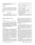
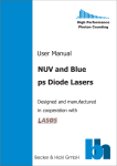
Becker & Hickl GmbH
Burst Analyzer 2.0
For Correlation Analysis and Single-Molecule Spectroscopy
FCS / FCCS – smFRET – PIE – ALEX – FILDA etc.
2nd Edition, March 2014
The Burst Analyzer Tutorial
Becker & Hickl GmbH
Nahmitzer Damm 30
12277 Berlin
Germany
Tel. +49 / 30 / 212 80 02 - 0
FAX +49 / 30 / 212 80 02 - 13
http://www.becker-hickl.com
e-mail: [email protected]
2nd Edition, February 2014
This handbook is subject to copyright. However, reproduction of small portions of the material in
scientific papers or other non-commercial publications is considered fair use under the copyright law.
It is requested that a complete citation be included in the publication. If you require confirmation,
please feel free to contact Becker & Hickl GmbH.
The Burst Analyzer Tutorial
Contents
1
Getting Started ........................................................................................................................... 1
1.1
What’s New in Version 2? .......................................................................................................... 1
1.2
System Requirements ................................................................................................................. 1
1.3
Installation .................................................................................................................................. 1
1.4
Getting Help................................................................................................................................ 2
2
Overview ..................................................................................................................................... 2
2.1
Visualizing Intensity Traces......................................................................................................... 3
2.2
Marking Bursts and Steps ........................................................................................................... 3
2.3
Generation of Time Curves Based On User Defined Functions .................................................. 4
2.4
Fluorescence Cross-Correlation Spectroscopy (FCCS, FCS) ........................................................ 4
2.4.1
User-defined fit functions for Fluorescence Correlation Spectroscopy ..................................... 5
2.4.2
Filtered FCS ................................................................................................................................. 5
2.5
Burst/Step Property Histograms ................................................................................................ 6
2.5.1
Lifetime Information (Fluorescence Decay Histogram).............................................................. 6
2.5.2
Lifetime Distributions ................................................................................................................. 6
2.5.3
FRET Histograms ......................................................................................................................... 7
3
Structure of Measurement Data (Macrotime and Microtime) .................................................. 8
3.1
Intensity Traces........................................................................................................................... 8
3.2
Microtime Histogram ................................................................................................................. 8
4
Software Description ................................................................................................................ 11
4.1
User Interface ........................................................................................................................... 11
4.1.1
Overview Diagram .................................................................................................................... 12
4.1.2
Measurement Data Diagram .................................................................................................... 12
4.1.3
Diagram of Auxiliary Functions ................................................................................................. 13
4.1.4
Microtime Histogram ............................................................................................................... 14
4.1.5
Project Panel ............................................................................................................................. 14
4.1.6
Menu Band ............................................................................................................................... 15
4.2
Data Files .................................................................................................................................. 15
4.3
Assigning Traces to Measurement Channels............................................................................ 16
4.4
Assigning Traces to Microtime Windows ................................................................................. 17
4.5
Correction of Traces ................................................................................................................. 18
4.6
Intensity Weighted Auxiliary Function ..................................................................................... 19
4.7
Creation of Bursts und Steps .................................................................................................... 19
I
The Burst Analyzer Tutorial
4.8
Attaching Properties to Bursts and Steps ................................................................................. 22
4.8.1
Intensity Property ..................................................................................................................... 23
4.8.2
Auxiliary Function Property ...................................................................................................... 23
4.8.3
Lifetime Property ...................................................................................................................... 23
4.8.4
ACF and CCF Properties ............................................................................................................ 24
5
Burst and Step Data Analysis .................................................................................................... 27
5.1
Property Data Tables ................................................................................................................ 27
5.2
Filtering ..................................................................................................................................... 28
5.3
Creating Histograms ................................................................................................................. 29
5.4
Histogram Options.................................................................................................................... 30
5.5
Examples ................................................................................................................................... 30
5.6
Saving and Exporting Histograms ............................................................................................. 33
6
Exporting Data .......................................................................................................................... 33
6.1
Importing Data into Matlab ...................................................................................................... 34
7
Glossary .................................................................................................................................... 36
The Burst Analyzer Tutorial
1 Getting Started
1.1 What’s New in Version 2?
1.
2.
3.
4.
5.
6.
7.
Multiple Table views of burst/step properties
Support for multiple filter sets
Histogramming of filtered burst/step properties
Huge speedup in FCS calculation
Exclusion of artefacts from FCS calculation
Automatic or manual recalculation of FCS data
FCS fitting with weights derived from raw single-photon data
1.2 System Requirements
Burst Analyzer can process projects of arbritary size as it creates an index file and only loads small parts
of the data on demand. It will run on any modern computer system, including laptop and netbook
systems. However, when large parts of a measurement are selected for viewing, memory size is
important.
Computer System (recommended): Intel Dual Core, 2 GHz or better, 2 GB RAM or better
Harddisk space: depends on amount of measurement data
Operating System: Windows XP SP3, Windows Vista, Windows 7, Windows 8, with .NET Framework
version 4.0 or higher installed.
1.3 Installation
1. Before install, make sure you have your license key ready.
2. Start Setup.exe from your installation media and follow the on-screen instructions.
3. For Windows 7 or earlier versions, Microsoft .NET Framework 4.0 must be installed. The setup
program will check the presence of the framework and install it if needed. After installing the .NET
framework, you have to reboot your computer and restart setup.exe.
4. When running Burst Analyzer for the first time, you will be asked for a license key. Please enter the
license key as written on your installation media.
If you do not see this dialog, click the Burst Analyzer Icon in the system tray.
If you want to change your serial number (e. g. if you have added other bh products to your license or
if you want to switch from a demo license to a full license, click
in the top right corner of the
application window. This will bring up an info window from where you can edit your license key.
1
The Burst Analyzer Tutorial
1.4 Getting Help
By clicking
you get access to the Burst Analyzer User’s Manual. It is a PDF document. To view it you
must have Adobe Acrobat Reader installed (or a similar PDF viewer). A click on “Help” will open the
manual in your PDF viewer.
Figure 1: Burst Analyzer Information Window. It shows contact information, software version number, license key and
gives you access to the user’s manual.
Burst Analyzer 2 comes with a number of tutorials which are accessible through the start menu. You
may also check the B&H website (www.becker-hickl.com) for application notes and other literature.
For an introduction into Fluorescence Correlation Spectroscopy, have a look at the following resource
by Petra Schwille and Elke Haustein: www.biophysics.org/Portals/1/PDFs/Education/schwille.pdf
2 Overview
BurstAnalyzer is a tool for analysis of time trace data. It can identify and analyze peaks in time traces
and also analyze user-defined time intervals. In addition to this, BurstAnalyzer can also perform
calculations on the full traces (e.g. compute auto-correlation or cross-correlation of time traces).
BurstAnalyzer has been specifically designed for analysis of data obtained from time-resolved singlemolecule fluorescence spectroscopy where a small focal volume is observed and a fluorescent
molecule entering the focus causes a large fluorescence burst. For this reason, time intervals in
BurstAnalyzer are called “Bursts”.
When a molecule changes its state it may also change its fluorescence properties. Such a (sudden)
change shows up as a step in fluorescence intensity. Thus, sub-regions of “Bursts” are called “Steps”.
Burst: Selection of arbitrary length within a fluorescence time trace. The common case is a peak in
fluorescence originating from a single molecule or a complex of molecules travelling through the
detection volume.
The Burst Analyzer Tutorial
Step: Selection of a time range within a burst. Normally, a step reflects a change of the properties
of a molecule while observed by the detection system.
1
2
Figure 2 Arbitrary time regions in an intensity trace can be selected for further analysis (1). These regions are called ‚bursts‘.
Sub-regions within bursts are called steps. (2) A burst containing two steps.
2.1 Visualizing Intensity Traces
The Burst Analyzer software helps you to visualize intensity traces from your single-molecule TCSPC
data fast and easily. Data from multiple detection channels can be combined into one trace or
separated by arrival time. Up to four different intensity traces can be defined. Burst Analyzer supports
automatic and manual selection of “bursts” from intensity traces and calculates several burst
properties automatically, such as mean fluorescence lifetime, intensity, auto-correlation and crosscorrelation. The various properties can then be further analyzed to determine molecular parameters,
such as molecule size and structure.
2.2 Marking Bursts and Steps
Arbitrary areas of intensity traces can be marked as “bursts”. Usually, a burst is a high-intensity region
of the trace indicating the diffusion of a molecule through the laser focus. Marking a burst is done by
just by clicking and drawing the mouse over the desired region, see Figure 3. As soon as the mouse
button is released, a burst is created and added to the project list together with its attached properties.
Each burst can be sub-divided into “steps”. Steps can be defined in the same way as the bursts but
must always start within a burst. Burst Analyzer provides numerous ways to analyze burst and step
data but it also possible to store burst properties within a project file and analyze them with external
software.
3
The Burst Analyzer Tutorial
1
2
3
Figure 3: Marking a burst in three steps: First, press the left mouse button at the desired start position of the burst.
Second, move the mouse while pressing the button to the desired end position of the burst. Third, release the button
to create the burst. The blue area turns into yellow and hence shows the localization of the burst.
2.3 Generation of Time Curves Based On User Defined Functions
Arbitrary functions of the signal intensity can be visualized. For example, a FRET trace is generated by
just entering the string “I2/(I1+I2)” as an 'auxiliary function'. The chart which shows this user-defined
function is always synchronized with the main data chart containing the underlying intensity traces
(see Figure 4).
1
2
3
Figure 4: On the basis of the user defined function string, an additional graph shows the outcome of the function which
uses the intensity values of the original trace by the parameter I1, I2, I3, and so on. In this manner, any auxiliary function
i.e. FRET traces can be generated and visualized together with the underlying intensity traces. A green background of
the textbox containing the auxiliary function string indicates an error-free function string.
2.4 Fluorescence Cross-Correlation Spectroscopy (FCCS, FCS)
The cross-correlation (CCF) function of two time-dependent signals f(t) and g(t) is defined as
G(tau) = <f(t)*g(t+tau)>/(<f(t)> * <g(t)>)
where <> denotes an average over the complete time range considered for calculation. If function f(t)
is correlated with itself (i. e. f(t)=g(t)), the result is called auto-correlation function (ACF). If f(t) and g(t)
are fluorescence signals, the functions are named FCS and FCCS, respectively.
In a typical FCS experiments, the sample is a dilute solution of molecules. Using a focused laser beam
for excitation a small focal volume of the solution is excited. Through confocal detection, the signal
from a femtoliter volume is collected. The average number of fluorescent molecules in the detection
volume is small and the molecules diffusing in and out of focus give rise to a fluorescence correlation
The Burst Analyzer Tutorial
function which is governed by the diffusion coefficient of the molecules, the shape of the detection
volume, the type of diffusion (e. g. two-dimensional or three-dimensional), etc.
With Burst Analyzer, you can compute and analyze FCS/FCCS curves from single-molecule TCSPC data.
Several predefined fitting models and user-defined functions are supported.
Figure 5 Left: Experimentally obtained auto correlation function of free Rhodamine 6G in solution (blue curve) overlayed
with the fit result of a model for freely diffusing particles (red curve). The model has three parameters: the number of
particles “N”, the diffusion time “tauDiff”, and the relation of the radii of the laser focus ellipsoid “omegaZ”. In the curve
Fluorescence Lifetime Distributions
2.4.1
User-defined fit functions for Fluorescence Correlation Spectroscopy
A software based correlation algorithm is implemented to generate auto and cross correlation
functions out of the TCSPC data stream of a user defined section of the traces. A Levenberg-Marquardt
fit algorithm adjusts the free parameters of a selected model. The results of the parameter values are
shown together with an overlaid function curve to show the quality of the fit, see Figure 6. While fitting
the data, the model parameters can be chosen to run free or to be hold fixed at their initial value.
Figure 6: Single Rhodamine6G in water. Upper: autocorrelation function (blue curve) with model (red curve). The model
parameters are listed in the right window and show the result of the curve fit.
The model itself is stored into a library of fit models which can be extended by user defined models.
All of these models can have an arbitrary number of parameters, where their name, initial value and
value bounds can be individually defined.
2.4.2
Filtered FCS
In Burst Analyzer, you can calculate a fluorescence correlation curve for a complete data set as well as
for particular regions within a data set. In addition to this, you can also filter a data set and exclude
selected regions (bursts) from analysis. This can be used to remove artifacts from FCS/FCCS
measurements.
5
The Burst Analyzer Tutorial
2.5 Burst/Step Property Histograms
2.5.1
Lifetime Information (Fluorescence Decay Histogram)
For TCSPC data, histograms of the measured photon arrival times are shown and automatically
updated based on the currently selected time interval within the data stream. The mean lifetimes for
all intensity traces are derived from the first moments of these histograms and are shown above the
decay chart.
The first moment is defined as m1   ti N i , where Ni is the number of counts in time channel i and t
i
is the time for the ith time channel, which results in the following lifetime estimate:
m 
t N /  N
i
i
i
i
i
In a typical experimental setup, the decay does not start at time t=0 but at a later time which is
determined by first moment of the system’s instrument response function. To get accurate lifetime
values, this offset value must be provided. It is recommended to set this to the maximum of the
fluorescence decay function. When you enter an offset, the maximum position is indicated as a
suggestion.
Figure 7: Histogram containing the lifetime information of the TCSCP data. An export function provides the histogram as
ASCII file to any further processing steps. The lifetime is calculated from the first moment of the decay data. An offset
correction can be provided.
2.5.2
Lifetime Distributions
The fluorescence lifetime can be calculated for each burst or step in an experiment. This data can be
used to show lifetime distributions within a sample.
Figure 8: Fluroescence lifetime distribution calculated form a large number of bursts coming from dextran molecules
labelled with Alexa 488. (Left) Two-dimensional histogram showing correlations between burst intensity and lifetime.
The Burst Analyzer Tutorial
2.5.3
FRET Histograms
With Burst Analyzer, you can analyze single-molecule FRET experiments. You can identify singlemolecule fluorescence bursts by specifying intensity thresholds for donor and acceptor channels. Thus,
you can separate bursts from interacting donor molecules from those which do not interact.
Figure 9: (Left) Donor lifetime distribution of a complex molecule labelled with CFP and YFP (simulated data). The histogram
shows 4 different FRET states. (Right) Two-dimensional histogram plot auf FRET efficiency obtained from donor and
acceptor intensities (“proximity factor”, (I2/(I1+I2)) vs. donor lifetime.
Based on your selection, you can then get FRET efficiencies by analyzing the donor lifetime or donoracceptor intensity ratios. In principle, both approaches should yield the same results. This is
demonstrated in Figure 9 where the FRET efficiency obtained from donor and acceptor intensities is
plotted versus the donor lifetime in a FRET experiment which shows multiple FRET states.
7
The Burst Analyzer Tutorial
3 Structure of Measurement Data (Macrotime and Microtime)
In a classic TCSPC measurement, photon arrival times are recorded. The time measurement is started
when a photon arrives at the detector and it is stopped when a laser pulse is detected. Thus, all photon
arrival times are measured with respect to an excitation pulse. This time difference can be recorded
very accurately but with this method there is no common reference point for all arrival times which
means the absolute arrival time of a photon (measured from the start of the experiment) is lost.
Modern TCSPC systems go one step further. In addition to the time difference between photon and
excitation pulse they also measure and register the absolute time from the start of the experiment.
Basically, they count the number of laser pulses from the start of the experiments and convert this
number into a time value which is possible because the lasers run at a constant repetition rate. This
arrival time is measured in units of the laser repetition rate. It is called “macrotime” while the time
between pulse and photon is called “microtime”.
3.1 Intensity Traces
In Burst Analyzer, the macrotime is used to generate fluorescence intensity traces. You can define a
time unit (e. g. 1 ms) and the number of photons within each successive time bin is counted and
displayed as a time trace. This shows how the fluorescence intensity changes over time.
In Burst Analyzer, the time trace analysis is based on the idea that whenever a fluoresceing molecule
crosses the laser focus, a burst of photons is emitted which gives rise to a peak in an intensity trace.
With Burst Analyzer you can find and analyzer such bursts in many different ways. You can use the
Burst Finder to identify bursts automatically or you can mark manually by simply using the mouse to
select an area in the intensity chart. This is done in the same manner as editing audio files with a wave
editor.
Figure 10: Measurement file with two spectral channels (blue and green) and one marked burst (yellow area).
Each photon arrival time is stored with routing information attached. The routing information usually
identifies a distinct detection channel from the measurement system. In Burst Analyzer routing
information is used to generate separate intensity traces for the detectors. In addition to this, you can
even split routing channels into multiple intensity traces by using the microtime information or
combine portions of different routing channels based on microtime.
3.2 Microtime Histogram
The microtime obtained from TCSPC experiments is the time difference between a photon and a
reference signal. In most configurations a pulsed laser is used to excite fluorescence and the microtime
is the time difference between the fluroescence signal and the excitation pulse. The measurement is
done in reversed start-stop configuration. This means that each recognized photon starts an internal
The Burst Analyzer Tutorial
timer which is stopped by the next recording of a laser pulse. To obtain a fluorescence decay profile
from the data it is only necessary to reverse the time scale of the microtimes before the microtime
histogram is built up.
In Burst Analyzer this is all done automatically and the histogram of microtimes directly shows the
probability of photon emission measured from the excitation pulse; see Figure 11 and Figure 12.
1200
Number of Photons
1000
=3.6 ns
800
600
400
200
0
0
5
10
15
20
Microtime (ns)
Figure 11: Theoretical distribution function of the photon arrival times of an excited state.
The excited state of a quantum system (i.e. the excited state of a single fluorophore species in a
uniform environment) with lifetime τ will emit photons in an autonomous random process at a
constant average rate of 1/. In this case the microtime distribution is mono-exponential. The only free
parameter of such a mono-exponential probability distribution is τ. For a mono-exponential
distribution this is equal to the first moment (or average arrival time) of the normalized photon
distribution:

 t F (t )dt  t exp(t /  )
1
µ1 ( F ) 
0

 F (t )dt
0


 exp(t /  )
However, due to the finite width of the laser pulse and the limited system response time of the
measurement electronics, the microtime histogram does not show the distribution of photon arrival
times of the excited state directly, but a convolution of this distribution with the instrument response
function.
9
The Burst Analyzer Tutorial
1
Number of Photons (a. u.)
Number of photons (a. u.)
1
0.8
0.6
0.4
0.2
0
0
5
10
Microtime (ns)
15
0.8
0.6
0.4
0.2
0
20 0
5
10
Microtime (ns)
15
Figure 12: Convolution of the mono-exponential photon distribution with instrument response of the detection system.
Left: instrument reponse (green, dotted) and exponential decay (red). Right: Convolution of exponential and instrument
response. The finite width of the system response is clearly visible in the rising part of the resulting curve (blue). The red
curve is a pure mono-exponential decay.

I (t )   F ( x) Irf (t  x)dx
0
It turns out that for a mono-exponential decay F(x) = exp(-x/tau),
µ1 ( I )   µ1 ( Irf ) .
This means you can obtain the true lifetime of the fluorophore by subtracting the first moment of the
(normalized) instrument response function from the first moment of the measurement data.
The system response function IRF can be recorded by feeding an attenuated back scattered laser beam
to the detector and recording a data set. The microtime histogram derived from this data set shows
the system response, the first moment of which must be subtracted from the lifetimes of the
measurement data to obtain the true lifetime values for fluorescence measurements. Therefore, the
software allows to define a constant offset value for each time trace to account for the influence of
the IRF.
Figure 13: A click on the round button at the right side of the lifetime information opens a menu where you can enter a
constant offset value which is subtracted automatically from the calculated first moment of the histogram to compensate
for the IRF.
20
The Burst Analyzer Tutorial
4 Software Description
All features of the software can be accessed from a set of toolbars. The active toolbar is selected by
selecting different 'tabs' in the top row of this menu band. Each toolbar contains subgroups of
elements with similar functionality. For example the dialog box for reading measurement files is
located in the first tab Start and then in the first group Data File. A click on the element Add SET/SPCFile opens the file open dialog.
Figure 14: The tool bar “Start”
In this manual, the position of the operational controls is specified as tab//group//element name. The
example from above reads Start//Data File//Add SET/SPC-File.
The data analysis approach of Burst Analyzer is based on marking certain areas of the data stream,
attaching property values to these areas and finally extracting information from a statistical analysis
of these properties.
The transition of a single molecule through the laser focus generates a photon burst, which can be
identified and marked manually by the Burst Analyzer software. This can be done for many bursts
yielding burst length statistics, which can be used to derive the distribution of sizes of the observed
molecules. This information can be saved in a project file. The project file stores the properties of the
marked areas only, and not the individual photon arrival times. The software keeps track of the burst
position within the raw data stream. This way, a correction of parameters, such as the background
level which deals directly with the raw data can be done with a simple click as the burst properties are
automatically recalculated from the raw data.
The project file is stored in an xml-format and is thus readable by any text editor. This facilitates further
data analysis with external tools. Programs like Matlab (Mathworks), IGOR Pro (WaveMetrics) or Origin
(OriginLab) can easily import the project files.
Identification of single-molecule bursts in the time traces of the data is the main functionality of Burst
Analyzer. Bursts can be marked manually or automatically by defining parameters such as minium and
maximum burst intensity. Furthermore, sub-areas of the bursts can be marked as 'steps'. This can be
useful as visible steps within a burst may correspond e. g. to certain conformational states of proteins.
Under appropriate circumstances, the changes inconformational states correspond to steps in the
FRET-trace and can be identified in this way.
4.1 User Interface
A screenshot of the user interface is shown in Figure 15. The user interface shows four measurement
panels (1 to 4) and a tree view with a listing of burst and step properties (panel 5). All control elements
are located in the head row (panel 6). Panel 1 shows an overview diagram; panel 2 holds the
measurement data as intensity time traces; panel 3 contains a diagram showing auxiliary functions,
11
The Burst Analyzer Tutorial
panel 4 contains a the microtime histogram, panel 5 the project window and panel 6 the active tab of
control elements.
6
3
5
1
2
4
Figure 15: The Burst Analyzer’s user interface. For explanations of the panels 1 to 6, see text.
4.1.1
Overview Diagram
The small diagram in the center contains an overview trace of the currently selected data set. The data
set can be selected by clicking a filename in the project panel (5).
The overview diagram displays the total intensity of all measurement channels as a function of
measurement time. Additionally this diagram shows the marked areas of bursts and steps in yellow.
Their absolute position in time can clearly be seen.
4.1.2
Measurement Data Diagram
Figure 16: This group of control elements provides user controls to set on and off the visibility of the intensity traces
and to determine the width of their time binning.
This diagram shows the photon arrival times in terms of up to four intensity traces. The visibility of the
individual time traces can be set by the four user control elements in Start//Traces Visibility, see Figure
16. The width of the time bins used for this diagram can be set through the Bin Width [ms] control
which is also located in the Start//Traces Visibility group. Values below 1 ms can be defined by decimal
values (using a decimal point, independent of the language settings), see Figure 16.
The Burst Analyzer Tutorial
The zoom area of the measurement data diagram can be moved using the elements in Start//Scroll and
resized with elements in Start//Zoom, see Figure 17.
Figure 17: Control elements for moving and scaling the visible area of the measurement data.
The zoom area is visualized as a blue rectangle in the overview diagram, see Figure 18. To move the
zoom area without rescaling the view, just click on the desired position in the overview diagram or
drag and drop the blue rectangle. Moving the mouse cursor on the edges of the blue rectangle will
resize the zoom area. Enlarging the width of the rectangle zooms out leading to increased memory
consumption due to a higher number of visualized photons. Shrinking the width zooms in yielding to
fewer data points and less memory demand.
Figure 18: Overview Diagram. The zooming area for panels 2, 3, and 4 is shown as a blue rectangle. Its size and position can
be changed directly by moving and squeezing it with the mouse. The measurement diagram will be updated accordingly.
4.1.3
Diagram of Auxiliary Functions
Panel 3 either shows a user defined function of up to four intensity traces or the correlation function
with a user defined fitting model. A cross-correlation or auto-correlation function can be shown.
The chart type can be chosen in the control group FCS//Curve Type, see Figure 19. If you select
“Auxiliary Function” you can define your own function by typing a string into a text box. In the function
definition “I1” to “I4” indicate the intensity values of the four available time traces. Showing the
“Auxiliary Function” is the default startup behavior.
or
or
Figure 19: Choosing the type of auxiliary chart: auto correlation, cross correlation or auxiliary function. Depending on the
selection, you can select the traces for correlation or enter the auxiliary function definition. In the “Auxiliary Function”
diagram each time bin is computed from the intensity values of the time traces within the bin using the function definition
you typed in. The default is to use “I2/(I1+I2)”. This is called proximity factor as it is related to the donor-acceptor distance
in a FRET experiment. As an example, the function string “(I2-I1)/(I2-2*I1)” gives you an anisotropy trace in case you
defined trace 1 as photons with parralel polarization and trace 2 as photons being perpendicularly polarized photons. For
assigning time traces to available routing channels see sections 4.3 Assigning Traces to Measurement Channels and section
4.4 Assigning Traces to Microtime Windows.
Within the function definition string, you can also use a few mathematical functions by entering e.g.
“Math.Log(I1/I2)”. The available mathematical functions are listed in Table 1 on p. 26.
The zoom area of the “Auxiliary Function” diagram is synchronized with the intensity traces of panel
2. Bursts and steps are visualized in yellow in both diagrams.
13
The Burst Analyzer Tutorial
If you choose “Auto Correlation” or “Cross Correlation”, the x axis in the diagram indicates the
correlation time and the graph displays a correlation function computed for the measurement data
shown in panel 2.
4.1.4
Microtime Histogram
This chart shows a histogram of photon arrival times for the photons within the currently selected time
range. In the border above the diagram, the lifetime information derived from the first moments of
the distributions is located, see Figure 20. Here, you can also define an offset to correct for an
instrument response which is not centered at t=0. Additional information about microtimes can be
found in section 3.2 Microtime Histogram.
Figure 20: Microtime Histogram. The first moment of the photon distribution gives an estimate of 4 ns for the lifetime. This
value must be corrected by subtracting the first moment of the instrument response. This offset can be defined for each
trace individually.
4.1.5
Project Panel
The Project Panel shows information on the active measurement project. It reflects the data stored in
the project file. The Project Panel has a tree structure with three hierarchical levels: files, bursts and
steps. Each file may contain bursts and each burst itself may contain steps. For each burst or step the
start time and length are shown. In addition to this tree structure, the project panel contains data
tables which show burst and step data separately. This lists are the basis for data analysis. They are
described in detail in section 5. The selection of burst and step properties shown in the project tab is
controlled by the settings in the Configuration tab, see section 3.1.6
Attaching Properties to Bursts and Steps is described from page 22 onward.
The Burst Analyzer Tutorial
file
steps
mean proximity factor
with standard deviation
burst
start
length
FCS fit
results
mean
intensities
Figure 21: Project panel. Files, bursts and steps compose the project tree. For each entry the “start” and “length” values
are shown. Additional parameters can also be attached to bursts and steps. In this example, bursts were generated with
additional mean intensities and FCS curve fitting results; while steps where configured to show proximity factor values.
The addition to the
4.1.6
Menu Band
The whole functionality of the software can be accessed by the elements in the menu band. They are
arranged in tabs. Each tab provides its own menu band containing groups of user controls. Figure 22
shows all user control elements of the current software version.
Figure 22: The menu band consists of four tabs: Start, Bursts, FCS and Configuration. Each of them provides user controls
arranged in groups.
4.2 Data Files
A set of measurement data consists of one .SET file and one to several .SPC files. If you have multiple
SPC modules in your measurement system, such set of files is created for each module. The SET file
saves the hardware settings of the measurement card and has a file size of a few kilobytes. The photon
15
The Burst Analyzer Tutorial
arrival times are stored into the .SPC files. The file size is proportional to the number of collected
photons. The typical file size is in the range of 10-100 megabytes. Depending on the measurement
parameters, all photons are either stored in one large SPC file or distributed over several smaller SPC
files. The number and size of .SPC files is not important when working with Burst Analyzer. In Burst
Analyzer, the photons are always loaded into the PC’s memory dynamically, even over the file borders
of several SPC files.
On a system with multiple measurement modules (i.e. SPC 154), it is sufficient to select only one of the
created SET files. The Burst Analyzer recognizes the number of modules automatically and adds the
relevant SET files to the set of measurement files.
The file open dialog is located at Start//Data File//Add SET/SPC-File. The first time that a data set is
opened, an index file is automatically created; this enables the concerted loading of the photons
corresponding to the currently selected zoom area without the need to scan all photon data. For every
SET file, an own index file will created, so every module gets its own index file. An index file has the file
extension “.idx”. Its file size is about 1/1000 of the sum of all attached SPC files. The IDX file is stored
in the same directory as the source SET and SPC data files. This means it is mandatory to have write
access to this directory. There is no further data processing possible without an existing index file.
Whenever it is missing, the Burst Analyzer automatically tries to create it.
4.3 Assigning Traces to Measurement Channels
In a typical measurement, photons from multiple detector channels are recorded. The detectors can
be connected to different recording channels of a multi-module TCSPC system, such as the SPC-154,
to the different inputs of a DPC-230 photon correlator board, or to a router attached to a single SPC
module. In most cases, different measurement channels have to be visualized by differently colored
time traces. With Burst Analyzer, time traces can be defined in an extremely flexible way. You can map
the photons from a measurement channel (or part of the photons based on the microtime) to one or
more time traces and you can define time traces which show the sum of different measurement
channels. The default setting in Burst Analyzer is to map the first four measurement channels to the
four available time traces. To display other measurement channels or do more a more sophisticated
selection based on the microtimes you have to change the trace definitions manually. This can be done
in the Time Trace Definitions dialog, located at Configuration//Time Traces//Settings.
A mouse click on the plus button opens a list of available measurement channels. With successive clicks
on the “+” button, you can add the photons from multiple measurement channels to one trace. A
mouse click on the “-“ button removes a measurement channel from a trace definition. See Figure 23
for an example. Here, a third time trace is generated from a two channel setup just by mapping both
measurement channels to the third trace as well.
Any of the four available traces can hold any number of measurement channels. However, every
attached channel increases the calculation time for the subsequent data processing algorithms like the
correlation function calculation.
The Burst Analyzer Tutorial
Figure 23: Two measurement channels were mapped to three time traces. Trace 1 (blue) shows photons from router 0,
trace 2 (green) is assigned to router 1, Trace 3 (orange) shows the photons of both traces and describes therefore the sum
intensity of both traces.
4.4 Assigning Traces to Microtime Windows
Using microtime information it is possible to split one measurement channel to different traces. In this
way, the FRET acceptor fluorophore in a scenario of a pulsed FRET experiment can be excited by a
second synchronized laser but recorded with the same detector as the donor fluorescence. As donor
and acceptor fluorescence show up in different parts of the microtime window, they can easily be
assigned to different time traces. Figure 24 shows an example configuration.
Figure 24: Measurement channel “Router 0” is assigned to Trace 1 (blue). Measurement channel “Router 1” is divided into
two traces based on its microtime information: “Trace 2” (green) and “Trace 3” (orange).
17
The Burst Analyzer Tutorial
4.5 Correction of Traces
In a typical experiment, the sensitivity of detectors can vary and the background level can also depend
on the wavelength and measurement channel. In Burst Analyzer you can correct for some of these
effects by assigning correction factors to the traces. For every trace there are two correction
parameters: a constant offset and a scaling factor. The offset value captures background noise, the
scaling factor reflects unequal detection efficiencies of the detectors. During calculation, the scaling
factor is processed first; afterwards the offset is subtracted. The background value must be given in
“counts/ms”. The parameters can be configured in the user dialog shown in Figure 25. The dialog is
located at Configuration//Corrections//Settings (see Figure 27).
Figure 25: The user dialog “Time Trace Noise Correction Parameter” provides two correction factors for every trace:
background subtraction and a scaling factor for detection efficiency compensation. The measured count rates will first be
multiplied with the scaling factor and afterwards corrected by subtracting the background offset value.
In more advanced setups with multiple detection channels, e. g. separated by a dichroic filter, a
fraction of an intensity signal may appear in the wrong channel due to an imperfect match of the
emission spectra of the fluorophore with the corresponding optical filters. With the crosstalk
parameter provided by the user dialog shown in Figure 26, the available time traces can be corrected
by the fraction originating from signal crosstalk. Like the “scale” parameter in Figure 25, the crosstalk
parameters are dimensionless relative factors of the source trace. The figure shows how to
compensate a crosstalk of 2% from channel 2 which falsely appears as a signal in channel 4.
Figure 26: The “Time Trace Crosstalk Correction Parameter” dialog gives access to options for signal cross talk correction.
The values entered represent a fraction of the source trace intensity showing up in the destination trace. The crosstalk
correction will be done first, afterwards the scale parameter will be processed, and at last the offset correction will be
applied.
The Burst Analyzer Tutorial
After setting the correction parameters, they must be activated by clicking the On element in the
Corrections control group (see Figure 27) and setting it to the 'On' state. Clicking On once more
will deactivate the corrections.
Figure 27: The user control group “Corrections” provides a user dialog for parameter settings and a toggle button “On” to
enable resp. disable the correction process.
4.6 Intensity Weighted Auxiliary Function
Using the Configuration//Aux. Func.//Intensity Weighted button (see Figure 22 on page 15), the time
bins involved in the calculation of mean and standard deviation of the auxiliary function for a burst (or
step) can be weighted by their intensity sum. . If the button is pressed, each involved time bin will have
a weight which is the total intensity of all intensity traces which are used in the auxiliary function string.
This way, time bins with higher count rates have more influence than time bins with low signal
intensity. If this option is not checked, each time bin is treated equally. For more information on
calculation of custom functions, see section 4.8.2 "Auxiliary Function Property" on page 23.
4.7 Creation of Bursts und Steps
Burst and steps can be created by marking a time area in the data chart with the mouse. A newly
marked area presents a burst; a newly marked area inside a burst presents a step. Bursts and steps will
automatically be added to the project and appear in the project panel with their start time and
duration and their additional attached properties, see section 4.1.5 Project . In addition to the time
consuming manual marking bursts can also be generated automatically in a very efficient way: The
menu band Bursts provides a set of user controls specifically for this purpose, see Figure 22.
Bursts//Auto Burst Finder//Settings presents a user dialog for configuring the thresholds for the burst
finder algorithm, see Figure 28 The automatic burst finder algorithm can be started by pressing the
Find Bursts button in the Bursts//Auto Burst Finder control group.
19
The Burst Analyzer Tutorial
Figure 28: User dialog for configuring thresholds for the automatic burst finder algorithm.
The first two parameters, “Min. Level” and “Flank Level” determine the size of the bursts. “Min. Level”
is the minimum count rates a burst must have. During the scan of the measurement data set, every
time bin will checked against this value. As soon as this value is reached, a burst is created with its start
value at this time bin and zero length. Next, the left and right border of this new burst will be extended,
until the current count rate drops below the “Flank Level” value of the corresponding trace.
Now, the burst created in this way will be checked against further parameters. “Min. AVG” and “Max.
AVG” are the minimum resp. maximum mean count rates of the entire burst. “Peak Level” is the
maximum value, which must not be exceeded for a time longer than that given by the “Peak Width”
parameter (in milliseconds). “Min. #Phot” and “Max. #Phot” are thresholds for the total number of
photons in a burst. A burst will be discarded, if one or more of the property values is outside of the
defined boundaries.
Each parameter can be activated or deactivated individually. The traces, on which the parameter
operates, can also be selected individually. Furthermore, each parameter can be linked between traces
with the settings “And”, “Or” or “Sum”. The setting of the link mode does only play a role, if more than
one trace is selected. The link mode “And” means, the threshold of the parameter must hold for all
traces, “Or” denotes, that the threshold may exceed only for one trace to turn the parameter check to
true. “Sum” indicates that the sum of the time bin values of all selected traces will be checked against
the parameter. For marking bursts, the parameter “Min. Level” is to be linked with “And” in order to
guarantee sufficient count rates for the selected traces. The parameter “Flank Level” can be best linked
with “Or”, cause the expansion of the burst should terminate as soon as the count rate in one trace
drops below the threshold value. All other parameter can be linked with “Or” in order to ensure that
a burst will not be added whenever one parameter in a trace does not fulfill the requirements.
There are three additional parameters in the Auto Burst Finder group of the menu band: “Min. Width”,
“Max. Width” and “Dark Width”, see Figure 29. “Min. Width” and “Max. Width” defines the borders of
The Burst Analyzer Tutorial
the tolerated burst length in Milliseconds. “Dark Width” allows a drop of the parameter “Flank Level”
for the configured duration. In this way, two adjacent bursts can be combined by increasing this
parameter.
Figure 29: The user control group “Auto Burst Finder” provides all parameters for the automatic burst finder algorithm.
Figure 30 demonstrates the burst finding process. The burst finder algorithm moves a marker from
time bin to time bin until the intensities of the current time bin exceed one of the defined “Min. Level”
thresholds. In Figure 30 this happened for the first time in this data stream at time 86979 ms. From
this position, a potential burst is initiated with start=86979 and width=0. Next, the left and the right
border will be extended, until the intensities of the current time bin falls below the thresholds “Flank
Level”. For subsequent burst detection, these two borders define a potentially new burst.
Figure 30: An automatically created burst with the parameters “Min. value”=50 for trace 1 (blue) and “Min. value”=40 for
trace 2 (green). “Flank level” was set to 10 for both traces. The burst detection started at position 86979 ms (red line).
After that, the borders are extended further until one intensity (Link=Or, resp. all intensites when
Link=And) are above the parameters “Flank Level” in the area of the length “Dark Width” around the
burst borders, see Figure 31. In this example, the “Link” property was set to “Or”, therefore only one
of the time traces was necessary to be continuously above its assigned “Flank Level”. In this example,
it was the green time trace 2. If “Link” was set to “And”, this condition should have hold true for each
trace. If “Link” was set to “Sum”, the sum of the corresponding traces should have been above the
threshold.
After the burst is defined in this manner, its properties will be determined and checked against all the
other parameters as described above. If one check fails, the burst will discarded. Otherwise, it will be
added to the project. Then, the burst finder will proceed until the end of the file or the maximum
number of bursts is reached. The maximum number of bursts can be set by the parameter
Bursts//General Parameter//Max #Bursts, see Figure 32.
21
The Burst Analyzer Tutorial
Dark Width
Flank Level
Figure 31: With the help of the parameter “Dark Width”, the burst was extended to its correct width. The red areas mark
the scanning regions where the intensities are continuously above “Flank level”.
Another way to automatically create bursts is to add bursts with a fixed burst width. In this case a burst
does not reflect a molecule diffusing through the focus but this mode can be useful to find out how
sample properties change over time within a measurement. The control group Bursts//Bursts with Fixed
Width contains user controls to define a burst width, add adjacent bursts with this width (in ms) or
equalize the burst width of all existing bursts automatically, see Figure 32.
Three further tools are available: automatically add one step per burst, delete all existing bursts and
delete all existing steps of the current data set. The value Max. #Bursts defines the maximum number
of automatically created bursts to prevent the creation of an unwanted amount of bursts in case of a
wrong parameter setting. The button Refresh all Bursts/Steps recalculates all property values attached
to bursts and steps, see section 0
Attaching Properties to Bursts and Steps. This may be necessary, e. g., after changing the correction
parameter. For configuring correction parameter see section 4.5 Correction of Traces.
Figure 32: Three control groups provide further automatic burst processing and step processing tools.
4.8 Attaching Properties to Bursts and Steps
There are five properties available to be attached to bursts and steps. They are called “Intensity”,
“Auxiliary Function”, “Lifetime”, “ACF” and “CCF”. They can be selected individually at
Configuration//Calculate Burst Properties and Configuration//Calculate Step Properties, see Figure 33.
The selected properties are calculated whenever a new burst or step is created, the borders of a burst
or step are changed or, when the Bursts//General Parameter//Refresh all Bursts/Steps button is clicked
(Figure 32).
The Burst Analyzer Tutorial
Figure 33: Attached Properties can be selected for bursts and steps individually. According to the settings made here, every
newly created burst will contain the mean intensity values of all available time traces and the fitting results of the auto
correlation function. Every new step will hold the mean value with standard deviation over his length of the user editable
auxiliary function.
Changing the selection of the properties does not affect existing bursts and steps. Therefore it is
possible, that a project contains bursts or steps with different sets of properties. With the user control
Bursts//General Parameter//Refresh all Bursts/Steps (see Figure 32), the sets of properties for all bursts
and steps within a project can be synchronized.
4.8.1
Intensity Property
When Intensity is selected, the mean intensity of each burst is stored together with the peak intensity
of the burst or step. This is done for all available time traces. All calculations are based on the corrected
time traces, see section 4.5 Correction of Traces. As soon as the parameter for the correction changes,
the attached properties should by updated. This can be done by clicking the Bursts//General
Parameter//Refresh all Bursts/Steps button, see Figure 32.
4.8.2
Auxiliary Function Property
By means of the user editable auxiliary function, a time trace of a user-defined function of signal
intensities can be generated , see section 4.1.3 Diagram of Auxiliary Functions. By selecting the
“Auxiliary Function” property, the mean value and its standard deviation of this auxiliary function will
be calculated and stored for each burst or step, respectively.
In this way, you can, for example calculate FRET efficiencies for steps by setting the function string to
“I2/(I1+I2)” (provided that I1 and I2 are acceptor and donor intensities). In this case, every step in the
project file contains its average FRET efficiency and standard deviation.
Note: All calculations are based on the background corrected count rates , see section 4.5 Correction
of Traces. Moreover, the values depend on the time bin size used for analyis, see section 4.1.2
Measurement Data. A larger time bin size leads to less fluctuations of the auxiliary function and thus
to reduced standard deviations.
If the button Configuration//Aux. Func.//Intensity Weighted (see Figure 22 on page 15) is checked, the
calculation of mean and deviation is weighted by the total intensity of the involved time traces within
each bin. Otherwise, each time bin is treated equally, see section 4.6 Intensity Weighted Auxiliary
Function.
4.8.3
Lifetime Property
If the Lifetime property is selected, the mean fluorescence lifetime will be calculated from the
microtime histograms of each new burst or step. The calculation is based on the first moment of the
microtime distribution and is carried out for all available data traces (see section 4.1.4 Microtime
23
The Burst Analyzer Tutorial
Histogram for more details). This can e. g. be used in FRET studies due to the fact that the donor lifetime
reduces with increasing FRET efficiency.
4.8.4
ACF and CCF Properties
If one of the properties ACF and CCF is selected, the auto correlation function (ACF) resp. the cross
correlation function (CCF) will be computed and fitted to the model selected in the FCS//Curve Fitting
group. The traces used for the calculation depend on the configuration in the Start//Auxiliary Chart
menu, see section 0 Fluorescence Correlation Spectroscopy (FCS/FCCS) for details. Note: the
computation time increases with the number of photons in a burst and can take some time especially
on slower computers. Fluorescence Correlation Spectroscopy (FCS/FCCS)
Fluorescence Correlation Spectroscopy is based on the analysis of temporal correlations within the
fluorescence signal. More specifically, FCS refers to the measurement analysis of the autocorrelation
function of a single intensity trace, whereas FCCS is based on the cross-correlation of two traces.
In a single-molecule experiment, the fluorescence correlation function reveals correlations between
individual fluorescence bursts resulting from single molecules or complexes of molecules diffusing
through the focal volume of the measurement system. From the resulting graph, one can see directly,
how the measured fluorescence signal is composed of correlated fluctuations of different lengths.
Large particles lead to a slow decrease of the FCS curve whereas small particles result in a fast decrease
of the FCS curve. The reason is that large molecules are diffusing much slower than smaller ones.
The correlation function for each burst or step is calculated numerically from the intensity signal
without any explicit assumptions about the measured molecules. For this, a multiple-tau algorithm is
used which uses logarithmically spaced groups of time bins (ref1). The correlation function is visualized
by Burst Analyzer as a blue curve in panel 3 (see fig. 29). The curve can be automatically fitted to an
appropriate model (i.e. freely diffusion particles of one type of equally sized and equally bright
particles). This is the first step where assumptions about the particles enter the analysis process. The
model parameters, i.e. mean number of particles or diffusion time, are determined through the fitting
process. The resulting fit function is shown as a red curve which is shown in the same diagram as the
correlation function. In this way, one can judge the goodness of fit at a glance, see Figure 34.
Figure 34: Left: Experimentally obtained auto correlation function of free Rhodamine 6G in solution (blue curve) overlayed
with the fit result of a model for freely diffusing particles (red curve). The model has three parameters: the number of
particles “N”, the diffusion time “tauDiff”, and the relation of the radii of the laser focus ellipsoid “omegaZ”. In the curve
1
S.Felekyan, R. Kühnemutz, V. Kudryavtsev, C. Sandhagen, W. Becker, C. A. M. Seidel, "Full correlation from
picoseconds to seconds by time-resolved and time-correlated single-photon detection", Rev. Sci. Instr., 76(8), p.
083104(2005)
The Burst Analyzer Tutorial
fitting window, initial values as well as lower and upper bounds can be set for each parameter. In addition, parameters
can also be fixed to user-defined values.
In the menu band of the main window, global parameters regarding FCS can be configured. The
correlation function is always computed using a logarithmic x-axis. The longer the underlying time
trace, the longer the highest possible x-value will be. The resolution of the correlation function can be
set by determining the number of points per cascade in FCS/General Parameter/Points per Casc., see
Figure 35. In the same control group, the range of the correlation time τ can be set. Initially, the lower
bound Start Corr. Func is set to 0 and the upper bound Stop Corr. Func is set to “Infinity” in order to
disable the effect of a restriction of τ.
Figure 35: The FCS menu band provides global settings concerning FCS/FCCS. The access to the fit function’s library is also
located here as well as the possibility to export the generated correlation function including its fit results.
In the Curve Fitting control group, the fit model can be selected. The fit can be done for a user-defined
interval of correlation time τ, which introduces the possibility to perform fits of only a part of the
numerical function, i.e. to achieve a tail fit. The lower bound is set with the control element Start, the
upper bound is defined by the element Stop.
There is a library containing models for free diffusion in two and three dimensions each with up to two
diffusion terms and up to one additional bunching term. It can be accessed by the control element
FCS/Curve Fitting/Library. The library can be extended by user defined functions as required, see Figure
36.
Figure 36: The fit functions library contains initially models for freely diffusion particles in two and three dimensions with
each up to three features. All of these models are editable. Moreover, further models can be added as required.
25
The Burst Analyzer Tutorial
To add a new function, first click the “+” button which adds a new entry to the end of the function list.
Select this entry and click the “Edit” button to open a new window which provides settings for the
function definition, see Figure 37.
A model consists of an arbitrary function name. This function name will appear in the list of available
functions. The list has a limited width; a reasonably short name should be chosen. Below the name,
the mathematical formula of the model can be entered. Any parameter names may appear here.
Nested brackets can be used at any depth. Moreover, mathematical functions can be called by using
the keyword “Math.” followed by the function name. For a complete list of supported math functions
see Table 1.
Table 1: Complete list of all supported mathematical functions of the function editor
Constants
E (2.71828, Euler number), Pi (3.14159, Circle number)
Trigonometric functions
Acos(radiant), Asin(radiant), Atan(radiant), Atan2(y, x),
Cos(radiant), Cosh(radiant), Sin(radiant), Sinh(radiant),
Tan(radiant), Tanh(radiant)
Exponential functions
Exp(number), Pow(base, exponent), Log(number), Log(number,
base), Log10(number)
Other
Abs(number), Sign(number), Min(number1, number2),
Max(number1, number2)
Rounding
Ceiling(number), Round(number), Truncate(number),
Floor(number)
Polynomial
Sqrt(number)
Please note: the function and variable names are case-sensitive.
Figure 37: Fit function definition window. This user interface provides the opportunity to define your own functions with
arbitrary names and function strings. The parameters involved can be extracted from the function string automatically
The Burst Analyzer Tutorial
(button Auto). Each parameter has a set of properties like name, initial value and bounds. If “fixed“ is checked, the
otherwise free parameter is set to the initial value and ignored by the fit algorithm.
As soon as the function string is error free the background color of the textbox turns from red to green.
The function is checked at every key stroke; there is no need to explicitly compile or check the function
string. New parameters can be introduced just by typing them into the function string. A click on the
“Auto” button afterwards extracts all parameters to the list in the lower part of the window and gives
the possibility to edit their properties. For every parameter, an initial value, lower and upper bounds
to restrict the value range during the fit and the setting “Fixed” is available. Whenever “Fixed” is
checked, the corresponding parameter will be turned into a constant and will not be optimized by the
fitting procedure. This may be advantageous if a model with many parameters does not converge. All
these parameter settings can also be accessed from the main window during the fitting process, see
Figure 34.
Note: the default variable name for the correlation time  is x.
A basic requirement for fit models is that the biochemical conditions do not change within the
observation time. The determination of the correlation function eventually represents a time average
of the observed time span. For a more detailed introduction into the method of fluorescence
correlation spectroscopy see ref2.
5 Burst and Step Data Analysis
5.1 Property Data Tables
When a burst or step has been defined, it will show up in the project tree and in the corresponding
data tables. You can select an item in the project tree or in a data table. The corresponding time trace
range will automatically be highlighted and centered in the trace view.
2
Medina, M. A., Schwille, P. Fluorescence correlation spectroscopy for the detection and study of single
molecules in biology, (2002) BioEssays, 24, 758–764.
27
The Burst Analyzer Tutorial
Figure 38 Project Tree and data lists in the single-molecule view. Data lists can be sorted by clicking a column header.
(Right) Many different filter criteria can be applied to a data set.
The data lists which contain all range properties are the basis for further analysis and visualization.
They contain all the different attached properties as individual data columns. You can plot various
histograms from each property and you can do this based on a number of filter criteria. Each data list
has its own set of filter conditions and it is possible to create multiple lists from the same raw data set.
All time related values in the lists are usually saved in milliseconds (except for the fluorescence
lifetimes which are given in nanoseconds).
Bursts and steps always contain “Start” and “Width” entries. All further entries appear only when the
corresponding property was selected during the creation of the burst or step, respectively.
The following entry identifiers exist:

Intensity: group containing average intensity values
o PhotonCount: mean intensity [counts per ms]
o PeakIntensity: maximum amplitude per bin [counts per ms]

AuxFunc: group containing means and deviations of the auxiliary function
o AuxiliaryFunctionName_Mean: mean value of the auxiliary function
o AuxiliaryFunctionName_Std: standard deviation of the auxiliary function

LifeTime: group containing lifetime information based on the lifetime histogram
o tau1, tau2, …: the lifetime value for every available time trace [ns]

ACF: group containing fit results of the autocorrelation function
o first entry: name of the choosen fitting function
o following entries: fitting parameter names with their fit results

CCF: group containing fit results of the crosscorrelation function
o first entry: name of the choosen fitting function
o following entries: fitting parameter names with their fit results
5.2 Filtering
Each data list is associated with a set of filter conditions which can be used to select a subset of items
for further analysis.
To add a filter condition,
1.
2.
3.
4.
5.
Click the “+” button in the top right corner of the table view.
Select the property you want to use for filtering
Specify minimum and/or maximum values
Click checkbox to enable filter
Click “Execute Filter” to apply all active filter conditions to the table.
The Burst Analyzer Tutorial
Add filter
Enable filter
Apply filter
Figure 39 Each data table can be filtered. Filter conditions can be added by clicking “+”. Filters can be activated and
deactivated by clicking a checkbox. Active filters are applied when “Execute Filter” is clicked.
Figure 40 Table entries which do not match the filter conditions are ‘greyed out’. They will not show up in data set
histograms.
To remove a filter condition,
1. Click “Del”
2. Click “Execute Filter”
Alternatively, you can deactivate a filter condition by unchecking the appropriate checkbox (see Figure
40).
5.3 Creating Histograms
The filtered data tables described in section 5.1 are the basis for further analysis. You can create 1- and
2-dimensional histograms from these data sets as well as create new data sets with different filter
conditions.
To create a histogram, you need to
1.
2.
3.
4.
Click the “+” button in the histograms bar.
Select the data set you want to use.
Select a property (or properties) for histogramming
Click “Ok” to apply your selection.
29
The Burst Analyzer Tutorial
Figure 41 To create a histogram, click the “+” button. You can create a standard 1D histogram from each column in a data
table. Or you can create a 2D histogram from each pair of columns.
5.4 Histogram Options
Figure 42 (Left) Settings for 1-dimensional histograms. (Right) Settings for 2-dimensional histograms
For each histogram, you can set the number of bins, and the minimum and maximum of the data range.
What you specify here is the center position of the first and last bin in each dimension. Clicking “Auto
(X) or “Auto (Y)” will determine these limits from the data.
For 1-dimensional histograms, “Auto (Y)” will automatically scale the y axis based on the histogram
data.
Most of the histogram settings can be changed after histogram creation. For this, simply right-click the
histogram area and make the changes. Click “Apply” when you are done.
5.5 Examples
In this section, we show a few example histograms and the corresponding histogram settings.
The Burst Analyzer Tutorial
Figure 43 1D fluorescence lifetime histogram with automatic scaling. The range is set to match the range of lifetimes in the
data set. (Auto(X) and Auto (Y) have been clicked.
Figure 44 Lifetime histogram with customized scale. Range limits and maximum have been entered manually.
31
The Burst Analyzer Tutorial
Figure 45 Lifetime (Channel 1) vs. Lifetime (Channel 2). Two-dimensional histogram. The color scale is set automatically.
The bin which contains most data points is black. Zero counts in a bin are shown in white.
The Burst Analyzer Tutorial
Figure 46 Two-dimensional histogram. By changing the number of bins per axis, you can create a histogram which
resembles a two-dimensional scatter plot.
5.6 Saving and Exporting Histograms
When you save a project, all histograms and data tables will be saved in the project file. When you load
a project file, the data sets and histograms are loaded from the file.
To create a bitmap file from a histogram, you have to
1. Right-click the histogram area.
2. Click “Save bitmap…”
This will bring up the following dialog:
Here, you can set the resolution and size of the bitmap. When you click “Ok”, you will be asked for a
filename.
6 Exporting Data
Starting from a burst analyzer project file with entries of bursts and steps, the data can be imported
by external software. Furthermore, the export function (see Figure 47: The project panel exhibits an
export button which saves the currently opened project file as an ascii file.) generates a project file in
a spreadsheet like shape with tabs and equal-signs as separator, therefore a direct import into Matlab
(Mathworks), Origin (OriginLab) or Excel (Microsoft) and similar software is possible. Averaging of time
slices over multiple experiments can be performed with one of these programs.
Figure 47: The project panel exhibits an export button which saves the currently opened project file as an ascii file.
33
The Burst Analyzer Tutorial
To import an ASCII project file in i. e. Excel, the column separator has to be set to the tab sign and
additionally to the equal sign “=”. Hereupon the cells of the spreadsheet will be filled with the data of
the project file. The first column is named with the type of the entry (“file”, “burst” or “step”); all other
columns are pairwise filled with the parameter name and the parameter value. Make sure to have the
decimal separator set to a point before importing the project file. Otherwise Excel will not well
recognize the number format.
The data set in the spreadsheet can now be used as a starting point for further analysis. A very common
task is to generate histograms of a subset of all data points. Let’s assume that we want to create a
histogram of the proximity factors of all steps, where the steps should have a minimum average
intensity of the second trace. To achieve that, sort the worksheet by the first column to accumulate all
steps to a contiguous range. Then, copy this range to a new worksheet and sort that new worksheet
by the desired property; In our example, this is the column containing the “PhotonCount2” entry. The
desired data points are now again in a contiguous range from which you can create a histogram with
Excel.
Project entries of different types, i.e. bursts and steps, can have different parameter sets. Their values
will occupy different columns. Furthermore, it may happen that even project entries of the same type
may exhibit different parameter sets. This situation can arise when the user changes the selection of
attached properties when some bursts or steps have already been created. To align all project entries
of the same type, the feature Bursts//General Parameter//Refresh all Bursts/Steps can be used to
update all project entries, which includes the alignment of their parameter sets. Afterwards, the
project file can be exported and processed further.
6.1 Importing Data into Matlab
ASCII data exported from BurstAnalyzer can easily be read by Matlab. We recommend to use the
following Matlab function
function [bursts steps] = baread(filename)
fid = fopen(filename);
bursts = struct([]);
steps = struct([]);
noOfBursts = 0;
noOfSteps = 0;
while ~feof(fid)
str = fgetl(fid);
C = textscan(str, '%s','Delimiter','\t');
b = C{1}{1};
switch b
case 'Burst'
noOfBursts = noOfBursts + 1;
bursts(noOfBursts).time = str2num(C{1}{2});
bursts(noOfBursts).width = str2num(C{1}{3});
[par ~] = size(C{1});
for i=4:par
parVal = textscan(C{1}{i}, '%[^=]=%f');
bursts(noOfBursts).(char(parVal{1})) = parVal{2};
end
case 'Step'
noOfSteps = noOfSteps + 1;
steps(noOfSteps).time = str2num(C{1}{2});
steps(noOfSteps).width = str2num(C{1}{3});
[par dummy] = size(C{1});
for i=4:par
The Burst Analyzer Tutorial
parVal = textscan(C{1}{i}, '%[^=]=%f');
steps(noOfSteps).(char(parVal{1})) = parVal{2};
end
end
end
fclose(fid);
end
The function bapxread returns two structure arrays corresponding to burst and step data. The fields
of the structures correspond to the various properties determined by Burst Analyzer and can be used
in any of the matlab plotting and analysis functions, e .g .
>> [burst step] = bapxread('myproject.txt');
>> hist([burst.width])
>> scatter([burst.width], [burst.tau1])
35
The Burst Analyzer Tutorial
7 Glossary
Burst
A burst is an aggregation of data points, here fluorescence photons. They indicate the presence of a
molecule near the center of the laser focus. The Burst Analyzer enables the user to mark any areas of
intensity traces. Those areas are called bursts due to the fact, that usually molecules in the laser focus
have to be marked. Bursts itself may contain () steps.
cw – continuous wave
A cw laser generates a continuous laser beam without interuptions in contrast to a pulsed laser, where
photons were emitted in periodic packages.
Data Set
A data set means the entity of information of one measurement which is stored into a set of multiple
files in different data formats. For identification of a data set, a SET file has to be specified here. It
contains internal links to binary files which store all the collected photon arrival times of the
measurement.
FCS – Fluorescence Correlation Spectroscopy
The data analysis is based on the correlation function of the measured time resolved fluorescence
intensity trace. This kind of spectroscopy is able to determine many physical parameters like i.e. the
size or the concentration of the investigated molecule. In contrast to other single molecule methods,
an intrinsic averaging over many molecules is performed.
FRET – Förster Resonance Energy Transfer
The energy of the excited state of a molecule can at appropriate conditions be transferred to an other
proximate molecule. This effect is very strong depandant from their mutual distance and arises
noticeably only at distances below 10 nanometers. The relation of the fluorescence intensities of an
adequate choosen pair of fluorophores reflects their mutual distance. This effect is thereby used to
measure inter fluorophore distances on the nanometer scale. Even more, with fluorophores attached
to known positions, the conformational dynamic of single molecules can be investigated with a high
temporal resolution.
Macrotime/Microtime
The time stamp of the photons consists of two times: the absolute laboratory time (Macrotime) and
the time duration since the preceded laser puls (Microtime). Out of the Macrotime, correlation
functions and intensity trajectories can be calculated. The microtime is used to extract the lifetime
information of the excited state.
Step
A () burst can hold sub areas which are called step. Usually these areas are defined to identify time
spans where the investigated molecule does not made a conformational change. This results in steps
in the FRET trace, which explains the name.
TCSPC – Time Correlated Single Photon Counting
TCSPC denotes the here used measurement method: single photons were not only counted but were
attached and stored with a very precise time stamp. The full temporal information of the detected
photon stream is reflected by the data.
The Burst Analyzer Tutorial
37