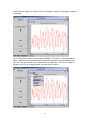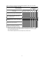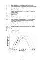
1
PHYGROW
(Phytomass Growth
Simulator)
User's Guide
Techical Documentation
Ranching Systems Group
Department of Rangeland Ecology and Management
Texas A&M University
Jerry Stuth, Dan Schmitt, R.C. Rowan,
Jay Angerer, and Kristen Zander
SEPTEMBER 2003
1
PHYGROW USER'S GUIDE
TABLE OF CONTENTS
I. INSTALLATION ................................................................................................3
II. RUNNING THE MODEL ..................................................................................7
III. PHYGROW INPUT PARAMETERS..............................................................13
IV. VIEWING RESULTS AND MANIPULATING GRAPHS ................................30
VI. EXPORTING DATA FOR FURTHER ANALYSIS.........................................36
APPENDIX A. .....................................................................................................40
APPENDIX B. .....................................................................................................47
APPENDIX C ......................................................................................................49
LITERATURE .....................................................................................................50
TECHNICAL GUIDE…………………………………………………………………. 51
2
PHYGROW Installation and User's Guide
I. Installation
To install PHYGROW on a machine from a CD, go to Windows Explorer or the My Computer icon
on the desktop. Double click on the CD drive letter. Double click on the folder named install,
then double click on the file named "Phygrow-2003-09-26.exe". Skip to step number 7 of this
section if installing from the CD. If you do not have a CD available with the Phygrow install, open
up Internet Explorer or Netscape after connecting to the Internet.
1. Go to http://cnrit.tamu.edu/phygrow.
Click on the Download link from the menu on the left of the screen.
3
Click on the word HERE in the screen to begin downloading the Phygrow model.
2. Click the HERE link in the main frame to begin downloading the PHYGROW model to the
local machine. The following screen will appear. Select the option to "Save this program to
disk" option.
3. Then click the OK button.
4
4. A "Save As" window will appear prompting for the location to save the file. Select a location
on the hard drive. The window captured below is saving the file to the "My Documents"
folder. It is important to know where the file was saved so that it can be executed or copied
onto a CD for other installs that need to be performed on machines that do not have access
to the Internet.
5. The setup file is called Phygrow-2003-09-26.exe. When the file begins downloading you will
see a status box appear like the one below, which indicates the progress of the download.
Depending on your connection speed, this can take from 1-5 minutes. Make sure the "Close
this dialog box when download completes" option is not checked during the download
process.
5
6. If you do not see a "Download Complete" window appear, when the progress bar reaches
100%, you must go to Windows Explorer or the My Computer icon, locate the folder where
you saved the installation, and double click the Phygrow-2003-09-26.exe file to begin. If you
do see the "Download Complete" window like the one below, click the Open button to begin
installation.
7. The Phygrow setup will prompt you for an installation folder. The default folder is C:/Program
Files/phygrow, which is shown below.
To accept the default folder click the Install button. To change the location of the Phygrow model,
highlight the text in to the left of the Browse button and indicate where the model should be
installed on the local machine.
6
8. The Phygrow Setup window will appear showing the progress of the files being copied from
the setup program to the hard disk. When the process is complete, the following window will
appear.
Click the Close button on this screen to complete installation.
II. Running the model
To start the Standalone Phygrow model, go to your desktop and double click on the icon that was
installed during installation.
A black screen will appear, which indicates that the client application is starting on the machine.
During startup the required files must be loaded for the Java application to run. This command
prompt screen gives you information regarding the success of this process.
7
After the model is loaded, a Java user interface will appear with a Window title of "Standalone
Phygrow" and "Common Modeling Environment" on the CME tab like the one below. You can
click the maximize window icon in the upper right hand corner (the middle button) to make the
window larger and more easy to view.
To begin a model run, click on the Models tab at the bottom of the interface.
8
This is the screen where you name the model run and select the host where the model is to be
executed. PHYGROW allows connections to remote servers configured for model runs. This
function speeds up processing times, and does not tie up resources on the client machine. In this
example, we will assume the client does not have access to a server running the Phygrow
backend process and run the model on the localhost. First, give the model run a name by placing
the cursor to the right of the Phygrow CSV button and typing in a descriptor for the site.
9
Then click the Phygrow CSV button. This means that you are going to run PHYGROW with a
parameter file of comma separated values, and that all of the information is saved in a single file.
The Phygrow CSV Parts button tells the model that you are going to perform a run with separate
comma separated value files for the soil, plant, grazer, and weather sections of the site. The
default installation, example video, and this user's guide reviews only the steps required to run
the model with a single file. Using the Phygrow CSV Parts function is an advanced feature of the
system and is beyond the scope of this manual.
This will take you to the Parameterize screen. Click on the maximize button.
10
Then go to File within the Phygrow CSV window, and select the word Load.
This will bring up the Open dialog box like the one shown below.
Double click on the data folder to open it. The default installation contains a parameter file for a
validation study done in Embrapa Pantana, South Maso Grosso State, Brazil, in which forage
standing crop estimates from PHYGROW were compared with data collected in grazing
11
experiments on 151 hectares. Select the campox3 file to load this validation study into the user
interface.
After the filename appears in the File Name text box, click the Open button to load the parameter
file into the window, as seen below.
12
The various parts of the parameter file are explained briefly in the demonstration video. The
parameter file can be modified in an external program such as Excel and saved as a comma
separated value, or CSV file, as indicated on the button within the user interface. Use the
param.txt file in the data directory of the installation as a template for creating a new parameter
file. After the file is created, load the parameter file into PHYGROW using the steps outlined
above and demonstrated in the video. The following section contains detailed explanations of
each parameter required to complete a PHYGROW run. Each of the parameters should be
entered into the appropriate place within the csv file, and must be filled out in order for the model
to execute and produce results. Click the OK button when you are ready to run the model.
III. PHYGROW INPUT PARAMETERS
1. Soil Attributes
A. Landscape Components
Surface Water Storage
This parameter defines the average depth to which water will pond in surface depressions during
a rainfall event when the soil is at saturation on the surface. It is a function of the percent of the
soil surface that ponds and the average depth of each surface depression. For instance, if 20%
of the soil surface ponds and average depth of the surface depressions are 1.0 cm then the
average depth is 0.2 cm. The water balance is sensitive to this variable as it influences the
amount of water that can infiltrate into the soil and also the amount of evaporation. Increases in
this number increase infiltration during large rainfall events.
This parameter can be derived from field observations or estimated by experts in the region.
Code variable name = furrow
units = cm
range = 0 to 50
precision = 0.01
Surface Slope
Slope is the number of meters of rise or fall in each 30 meters of land and is expressed in
percent. This value influences infiltration and runoff. For PHYGROW, the slope given for the soil
series should be used. For field situations where the soil information cannot be found, use the
average slope of the site being parameterized.
code variable name = slope
units = percent
range = 0 to 100
precision = 0.1
Max SCS Condition Curve Number
The maximum value of the SCS condition curve number for the parameterized soil given the
cover type and hydrologic condition. The SCS Runoff Curve Number (CN) method is used to
determine water runoff in the model. This method is described in detail in NEH-4 (SCS 1985).
The major factors that determine CN are the hydrologic soil group (HSG), cover type, treatment,
hydrologic condition, and antecedent runoff condition. See Appendix A, tables 1 and 2 for
suggested curve numbers for rangeland cover types for various hydrological groups and
hydrological conditions.
code variable name = scsc
units = none
range = 0 to 150
precision = 1
13
Min SCS Condition Curve Number
The minimum value of the SCS condition curve number for the parameterized soil given the cover
type and hydrologic condition. The SCS Runoff Curve Number (CN) method is used to determine
water runoff in the model. This method is described in detail in NEH-4 (SCS 1985). The major
factors that determine CN are the hydrologic soil group (HSG), cover type, treatment, hydrologic
condition, and antecedent runoff condition. See Appendix A, tables 1 and 2 for suggested curve
numbers for rangeland cover types for various hydrological groups and hydrological conditions.
code variable name = minscsc
units = none
range = 0 to 150
precision = 1
Bottom type
This parameter defines the conditions below the bottom most layer of parameterized soil.
following codes are used to define the condition
Bottom type = 0
Bottom type = 1
Bottom type = 2
The
Bottom is permeable (unconsolidated material, water drains freely)
Bottom is impermeable (rock or indurated layer, allows water to perch)
Bottom is a water table (water is present at all times)
code variable name = bottom
units = none
range = 0 to 2
precision = 1
B. Soil Layer Components
Soil Name
User defined name for each layer of the soil that is being parameterized. Name can be
alphanumeric, but must not contain any of the following: =,+,*<,>,-,/,or %.
code variable name = name
units = none
range = n/a
precision = n/a
Rock Factor
The volume of rock fragments (unattached pieces of rock 2 mm in diameter or larger) that are
present in the soil layer. It is a ratio of the volume of rock fragments to the total volume of the
layer. It is commonly determined as part of field and laboratory analyses for soil surveys and can
be found in the attribute data for published soil surveys. This parameter directly influences the
soil water holding capacity and therefore, plant available water. Increases in this parameter
decrease plant available water.
code variable name = rockfactor
units = cm3/cm3
range = 0 to 1
precision = 0.001
Saturated Hydraulic Conductivity
This parameter relates the soil water flow rate (flux density) to the hydraulic gradient and is a
measure of the ease of water movement in soil. Saturated hydraulic conductivity is the reciprocal
of the resistance of soil to water movement. As the resistance increases, the hydraulic
14
conductivity decreases. Resistance to water movement in saturated soil is primarily a function of
the arrangement and size distribution of pores. Large, continuous pores have a lower resistance
to flow (and thus a higher conductivity) than small or discontinuous pores. Soils with high clay
content generally have lower hydraulic conductivities than sandy soils because the pore size
distribution in sandy soil favors large pores even though sandy soils usually have higher bulk
densities and lower total porosities (total pore space) than clayey soils. Data from this parameter
can be found in laboratory data for the soil series provided by the NRCS. Appendix Table 3 can
also be used as a guideline when laboratory data are not available. The Soil Water
Characteristics Hydrologic Properties Calculator developed by Washington State University
(http://www.bsyse.wsu.edu/saxton/soilwater/) is also helpful in determining this parameter when
laboratory data are not available.
In the PHYGROW model, this is a primary variable influencing water movement into the soil via
infiltration and subsequent movement of water through layers under saturated conditions.
code variable name = hydrConduct
units = cm/hr
range = 0 to 100
precision = 0.005
Bulk Density
The bulk density parameter is defined as the mass of oven-dry soil per unit (grams) divided by the
total volume of soil (cm3) at a water tension of -1/10 bar or -1/3 bar. It is commonly measured
during field soil surveys or determined from field collected soil peds sent to a laboratory. It is
commonly reported in attribute data published by NRCS for each layer in a soil series. In the
absence of field collected or laboratory data, Appendix A Table 4 can be used as a guideline.
The Soil Water Characteristics Hydrologic Properties Calculator developed by Washington State
University (http://www.bsyse.wsu.edu/saxton/soilwater/) is also helpful in determining this
parameter when laboratory data are not available.
In the model, this parameter influences crack flow and water holding capacity.
code variable name = bulkD
units = g/cm3
range = 0 to 5
precision = 0.001
Volumetric Water Content at 0 Bar
This parameter represents the total possible water content of the soil when the soil is completely
saturated. In PHYGROW, it represents the volume of water in the soil at saturation (i.e. all pore
spaces are full) without rocks included. During the calculation of the available water in
PHYGROW, the rock fragments (rock factor above) are included into the calculation so that their
effect on the water availability is accounted for. Volumetric water content is generally measured
in the laboratory from samples collected during a field soil survey. In the absence of laboratory
data, Appendix Table 5 can be used for a guideline if texture is known. The Soil Water
Characteristics Hydrologic Properties Calculator developed by Washington State University
(http://www.bsyse.wsu.edu/saxton/soilwater/) is also helpful in determining this parameter when
laboratory data are not available.
code variable name = volWater0
units = cm3/cm3
range = 0 to 1
precision = 0.001
Volumetric Water Content at -1/3 Bar
15
This parameter represents the water content of the soil when the water is held in the soil at –1/3
bar of tension, also known as field capacity. Field capacity is defined as the volume of water
remaining in a soil 2 or 3 days after having been wetted with water and after free drainage is
negligible.
As with Volumetric Water Content at 0 bars, the rock fragments (rock factor above) are included
into the calculation of this parameter in PHYGROW so that their effect on the water availability is
accounted for. Volumetric water content is generally measured in the laboratory from samples
collected during a field soil survey. In the absence of laboratory data, Appendix A Table 5 can be
used for a guideline if texture is known. The Soil Water Characteristics Hydrologic Properties
Calculator developed by Washington State University
(http://www.bsyse.wsu.edu/saxton/soilwater/) is also helpful in determining this parameter when
laboratory data are not available.
code variable name = volWater-.333
units = cm3/cm3
range = 0 to 1
precision = 0.001
Volumetric Water Content at -15 Bar
This parameter represents the water content of the soil when the water is held in the soil at –15
bars of tension, also known as permanent wilting point. Permanent wilting point is defined water
content of a soil at which indicator plants, growing in that soil, wilt and fail to recover when placed
in a humid chamber.
As with Volumetric Water Content at 0 bars, the rock fragments (rock factor above) are included
into the calculation of this parameter in PHYGROW so that their effect on the water availability is
accounted for. Volumetric water content is generally measured in the laboratory from samples
collected during a field soil survey. In the absence of laboratory data, Appendix Table 5 can be
used for a guideline if texture is known. The Soil Water Characteristics Hydrologic Properties
Calculator developed by Washington State University
(http://www.bsyse.wsu.edu/saxton/soilwater/) is also helpful in determining this parameter when
laboratory data are not available.
code variable name = volWater-15
units = cm3/cm3
range = 0 to 1
precision = 0.001
Dry Bulk Density
The dry bulk density parameter is defined as the mass of oven-dry soil per unit (grams) divided by
the total volume of soil (cm3) at a water tension -15 bars. It is not commonly measured during
field soil surveys, but is sometimes determined in the laboratory. In the absence of data for this
parameter, use the bulk density parameter above or use the Map Unit User File (MUUF) program
(http://www.wcc.nrcs.usda.gov/wetdrain/wetdrain-tools.html) for estimating this given a soil series
name.
In PHYGROW this parameter influences soil cracking, thus influencing infiltration and macropore
movement of water.
code variable name = DrybulkD
units = g/cm3
range = 0 to 5
precision = 0.001
2. Plant Attributes
16
A. Site Specific Components
Plant Name
User defined name for plant species that is being parameterized. Name can be alphanumeric,
but must not contain any of the following: =,+,*,<,>,-,/,or %. Generally, a species code that is
linked to a database, common names, or latin names are used.
code variable name = plantfl
units = n/a
range = n/a
precision = n/a
Initial Standing Crop
This parameter defines the initial standing crop (kg/ha) for the species being parameterized for
the starting day of the model run. This variable can be estimated from, or measured during a field
survey of species being modeled. For long term (> 5 years) simulations, the model is not
sensitive to this parameter. However, an accurate representation of this number would be
required for short term simulations. (Note: this parameter should not exceed the value obtained
when multiplying the decimal percent of maximum expression times the maximum aboveground
biomass).
code variable name = initialSC
units = kg/ha
range = 0 to 1000000
precision = 0.01
Percentage of Maximum Expression
This parameter reflects the percent of potential niche occupancy that a species is currently
expressing in a plant community. For herbaceous species this is determined using a
representative stand that is sampled for grass basal cover (%), forb frequency (% in a 5 x 5 cm
frame) and effective woody plant canopy cover (%). The preferable method for gathering data for
this parameter is field collection on a transect using a modified point frame. However, historical
cover data or expert knowledge can be used to define the relative proportions of the species
being simulated. The model is sensitive to this parameter as it defines the proportionality of an
individual species compared to its site potential along with its proportionality to the species that
are competing with it on the site.
code variable name = percentMax
units = decimal percent
range = 0 to 100
precision = 0.001
Site Nutrient Factor
This parameter is used as a scalar to increase or decrease the growth rate for a species due to
increased or decreased nutrients or climate change. In most cases, this value should be set to 1,
meaning no change in growth. Values greater than 1 will have proportional increases in the
growth rate to the value entered. Values less than 1 will decrease growth rate proportionally.
code variable name = nutrientFactor
units = n/a
range = 0.01 to 2
precision = 0.01
B. Species Specific Parameters
17
LAI Leaf Area Index
Leaf area index (LAI) is ratio of the total area of all leaves on a plant to the area of ground
covered by the plant. It is an important structural property of a plant canopy because it defines
the number of equivalent layers of leaves the vegetation displays relative to a unit ground area,
thus defining the photosynthetic area, as well as water interception area of the species being
simulated. The data for this parameter can be gathered from field surveys or published reports
and literature. Field data collection requires collection of leaves from a species within a known
ground area. The collected leaves are then fed into a scanning device that measures the area of
the leaves. Leaf area can then be determined by dividing the scanned leaf area by the ground
area. Leaf area is commonly measured in water balance and photosynthesis studies. The Oak
Ridge National Laboratory has a compilation of the leaf area index for over 1000 species and can
be accessed at this web address http://www.daac.ornl.gov/VEGETATION/lai_des.html.
PHYGROW is sensitive to this parameter because it defines the leaf area available for
photosynthesis, thus influencing plant growth for the species being simulated. Interception loss
is also influenced by this parameter as it defines the area of the plant that has the potential to
intercept rainfall.
code variable name = LAI
units = ratio
range = 0 to 60
precision = 0.01
Dry Matter to Radiation Ratio
This parameter defines the efficiency to which the plant converts radiation into biomass.
Mathematically it is the slope of the linear relationship between biomass production and
photosynthetically active radiation (PAR) intercepted by the canopy. It is commonly determined
in plant growth experiments and is a parameter in many plant growth models. Data for this
variable can be gathered from field experiments, however specialized equipment is needed to
measure PAR and data must be collected over a period of time to develop the relationship.
Published values can be found in the literature for many forage and rangeland species. Appendix
Table 6, provides Dry Matter to Radiation ratios that can be used for these same or similar
species in PHYGROW.
PHYGROW is sensitive to this parameter as is controls the amount of biomass that a species can
grow each day. As biomass accumulates, so does leaf area index and wood (in woody plants
only), thus further increasing the potential for growth.
code variable name = BioCvt
units = grams/Megajoule
range = 0 to 6
precision = 0.01
Suppression Temperature
This parameter defines the maximum temperature at which a species can grow. Beyond this
temperature plant growth will cease in the model. Information on this parameter can be gathered
from published literature for the species or from online databases such as ECOCROP
(http://ecocrop.fao.org). If published values are not available, Appendix A table 7 can be used as
a general reference.
The plant growth curve in PHYGROW is sensitive to this number as it defines the end point of the
growth curve.
code variable name = supTemp
18
units = Celsius
range = 0 to 60
precision = 0.01
Base Temperature
This parameter defines the minimum temperature at which a species can grow. Below this
temperature plant growth will cease in the model. Information on this parameter can be gathered
from published literature for the species or from online databases such as ECOCROP
(http://ecocrop.fao.org). If published values are not available, Appendix A table 7 can be used as
a general reference.
The plant growth curve in PHYGROW is sensitive to this number as it defines the starting point of
the growth curve.
code variable name = baseTemp
units = Celsius
range = -10 to 60
precision = 0.01
Optimum Temperature
This parameter defines the optimum temperature at which a species will grow. Above or below
this temperature plant growth will incrementally decline as the base temperature or the
suppression temperature are approached. Information on this parameter can be gathered from
published literature for the species or from online databases such as ECOCROP
(http://ecocrop.fao.org). If published values are not available, Appendix A table 7 can be used as
a general reference.
The plant growth curve in PHYGROW is sensitive to this number as it defines the point where
maximum growth under water non-limiting conditions would occur. Changes in this parameter will
lead to shifts in the growth curve.
code variable name = optTemp
units = Celsius
range = -10 to 60
precision = 0.01
Left Side of Temperature Curve
This parameter defines the left curve shape for parameterization of a Poisson Density Function
curve to simulate temperature effect on growth. Values for the left side of the curve can range
from 1 to 5. A value of 1 makes the curve side more spread out. A value of 5 makes the curve
side thin and skewed toward the midpoint. Appendix table 7 provides several examples of this
number for several species.
code variable name = leftTempCurve
units = none
range = 0 to 5
precision = 0.1
Right Side of Temperature Curve
This parameter defines the right curve shape for parameterization of a Poisson Density Function
curve to simulate temperature effect on growth. Values for the left side of the curve can range
from 1 to 5. A value of 1 makes the curve side more spread out. A value of 5 makes the curve
side thin and skewed toward the midpoint. Appendix table 7 provides several examples of this
number for several species.
code variable name = rightTemp Curve
19
units = none
range = 0 to 10
precision = 0.1
Leaf Green to Dead Rate
Leaf green to dead rate is the percentage of the total green leaf biomass that is transferred to
standing dead leaf biomass on a daily basis when leaves are actively growing. In field situations
this can be determined from leaf mapping or leaf marking techniques followed over a period of
time. It can also be estimated from scientific studies where litter fall and leaf turnover have been
measured.
In PHYGROW, this is an extremely sensitive variable, especially for woody plants. Values that
are too high can lead to too much standing dead biomass and a lack of photosynthetic material.
Default values of 3 are suggested for grasses and forbs, 1.75 for deciduous woody species, and
a value of 1 for evergreen species.
code variable name = greentoDead
units = percent
range = 0 to 10
precision = 0.01
Leaf Green to Dead Rate During Dormancy
This parameter defines the percentage of total green biomass that is transferred to standing dead
leaf biomass on a daily basis when leaves are dormant due to temperature or water stress. In
field situations this can be determined from leaf mapping or leaf marking techniques followed over
a period of time. It can also be estimated from scientific studies where litterfall and leaf turnover
have been measured.
In PHYGROW, this is sensitive variable, but not as sensitive to growth as the leaf green to dead
rate described previously. Default values of 2.5 are suggested for grasses and forbs, 1.5 for
deciduous woody species, and a value of 0.5 for evergreen species.
code variable name = dormlturn
units = percent
range = 0 to 10
precision = 0.01
Leaf Turnover
Leaf turnover expresses the daily loss of leaf biomass that occurs from the total standing dead
pool to the leaf litter biomass pool. In field situations this can be determined from leaf mapping or
leaf marking techniques followed over a period of time. It can also be estimated from scientific
studies where litterfall and leaf turnover have been measured.
In PHYGROW, this is a sensitive variable. Values that are too high can lead to too much litter
biomass and values that are too low can lead to a build up of standing dead biomass. Default
values of 3 are suggested for grasses and forbs, 1.75 for deciduous woody species, and a value
of 1 for evergreen species.
code variable name = lturnOver
units = Percent
range = 0 to 100
precision = 0.01
Heat Unit Accumulation at Seed
The growth and development of annual plants in PHYGROW is regulated by accumulated heat
units. Heat units are the positive increments of differences between the base temperature and
20
average daily temperature of the simulation. The Heat Unit Accumulation at Seed defines the
number of heat units that need be accumulated before the species can set seed. This can be
determined from published literature for the species in question or determined from field
measurements. For species that are not annuals, this value should be set to 0.
code variable name = huiSeed
units = Celsius
range = 0 to 2000
precision = 10.
Heat Unit Accumulation at Death
The Heat Unit Accumulation at Death defines the number of heat units that need be accumulated
before the species will die under water non-limiting conditions. This can be determined from
published literature for the species in question or determined from field measurements. For
species that are not annuals, this value should be set to 0.
code variable name = huiDead
units = Celcius
range = 0 to 2000
precision = 10.
Rooting Depth
Rooting depth defines the maximum rooting depth of the species under non-water stress
conditions on the site that is being parameterized. This parameter can be determined from
published values in the literature or field experiments. Online databases such as ECOCROP
(http://ecocrop.fao.org) also provide information on this for some of the species catalogued.
code variable name = rootDepth
units = cm
range = 0 to 10000
precision = 1.
Canopy Height
Canopy height defines the maximum canopy height of the species under non-water stress
conditions on the site being parameterized. This parameter can be determined from published
values in the literature or from direct measurements in the field. Online databases such as
ECOCROP (http://ecocrop.fao.org) also provide information on this for some of the species
catalogued.
code variable name = canopyHeight
units = cm
range = 0 to 100000
precision = 1.
Maximum Above Ground Biomass
This attribute establishes the maximum amount of biomass (both wood and leaf) for a species on
the site being simulated under optimal growth conditions. This parameter can be determined
from published values in the literature or from direct measurements in the field. Online databases
such as ECOCROP (http://ecocrop.fao.org) also provide information on this for some of the
species catalogued.
This is an important variable in PHYGROW because it established the maximum productivity of a
species on a site. Incremental changes in this number will subsequently lead to incremental
changes in the standing crop of the species being simulated.
code variable name = maxWeight
21
units = kg/ha
range = 0 to 500000
precision = 1.
Leaf/Above Ground Biomass Ratio
This parameter defines the ratio of leaf biomass to total above ground biomass (kg leaf /kg total
biomass). It is important for partitioning out leaf biomass and wood biomass. For grasses,
sedges, and non-woody dicots, this value should be set to 1. For shrubs, trees and woody forbs,
this value can range from 0.03 to 0.95. Information to derive this parameter can be gathered from
published literature where biomass components have been separated and weighed. In field
surveys, whole plants can be collected and leaf and wood material can be separated, oven dried,
and weighed to derive this variable.
code variable name = leafRatio
units = ratio
range = 0 to 1
precision = 0.005
SAI Stem Area Index
Stem area index (SAI) is ratio of the total area of all woody stems on a plant to the area of ground
covered by the plant. Data for this parameter can be collected in much the same way as leaf
area index described above. It is generally not collected during field surveys, and published
values for this in the literature are rare. . A default value of 10% of leaf area index (LAI – defined
above) can be used in situations where you cannot measure this parameter. In PHYGROW, this
parameter influences the amount of throughfall, stemflow and interception loss. Forage
production is relatively insensitive to changes in this value.
code variable name = SAI
units = ratio
range = 0 to 1
precision = 0.01
Leaf Water Store Capacity
This parameter defines the amount of water (grams) that adheres to the surface of the leaves and
then evaporates into the atmosphere. Data for this parameter can be gathered in field surveys
where current year’s growth (leaves and new stem growth) are collected and weighed. Leaves
and new stem growth are then dipped in water or sprayed until saturated. They are then shaken
3 times and weighed again. The difference between the two weights represents the weight of
water sticking to the leaves that will evaporate back into the atmosphere. The plant tissue is then
placed in an oven to derive dry matter weight and allow the adhesion to be expressed as g water
per g dry matter. Published values for this are rare in the literature. Forage production in
PHGYROW is relatively insensitive to this parameter as it mostly affects interception loss in the
water balance.
code variable name = leafStore
units = grams water/gram dry matter
range = 0 to 5
precision = 0.001
Stem Water Store Capacity
This parameter defines the amount of water (grams) that adheres to the surface of the wood and
then evaporates into the atmosphere. Data for this parameter can be gathered in much the same
way as that described for leaf material above. Forage production in PHGYROW is relatively
insensitive to this parameter as it mostly affects stemflow in the water balance.
code variable name = stemStore
22
units = grams water/gram dry matter
range = 0 to 5
precision = 0.001
Fraction of Water Transferred from Leaf to Stem
This parameter defines the amount of water captured by the leaf canopy in excess of leaf storage
capacity that will either drip off the end of the leaf or flow down the woody stem. It is the fraction
of the total amount of water that travels from leaf to woody stem. Published values are rare for
this in the literature and it is hard to determine during field surveys. A proxy value for this can be
determined from water balance studies where stemflow has been collected. One can take total
stemflow and divide it by total incident precipitation to derive a value for this parameter. Forage
production in PHGYROW is relatively insensitive to this parameter as it mostly affects stemflow in
the water balance.
code variable name = stemDrip
units = proportion
range = 0 to 1
precision = 0.01
Stem Turnover
This variable is the percent wood biomass that turns over to the litter pool each day expressed as
a percent of current standing wood biomass. In field situations this can be determined from stem
mapping or stem marking techniques followed over a period of time. It can also be estimated
from scientific studies where litterfall and stem turnover have been measured.
In PHYGROW, this is a sensitive variable. This parameter defines the daily loss of woody
material from the canopy. Values that are too high can lead to too much stem litter biomass and
values that are too low can lead to over production of woody material in the simulation. Initial
values of 0.01 to 0.1 are suggested for most woody species.
code variable name = sturnOver
units = percent
range = 0 to 5
precision = 0.005
Cold Unit Accumulation to Freeze Leaf Damage
This parameter is defined as the accumulated negative differences between current days average
temperature minus the base temperature. The susceptibility of tissue death is a result of a certain
amount of cold accumulated below the base temperature. Generally, observation of killing frost
and computation of temperatures that occurred during the event is the best way to compute this
variable. Data can also be obtained from published literature.
code variable name = cuaFreeze
units = Celcius
range = 0 to 2000
precision = 10.
Canopy Base Diameter
This is the maximum canopy diameter at the base of the plant canopy at peak expression under
optimal conditions at the site being simulated. It can be determined from direct measurement or
published literature.
code variable name = cbasedia
units = cm
23
range = 0 to 50000
precision = 1.0
Canopy Crown Diameter
This is the maximum canopy diameter expected by the plant at peak expression under optimal
conditions at the site being simulated. It can be determined from direct measurement or
published literature.
code variable name = ccrowndia
units = cm
range = 0 to 50000
precision = 1.0
Height at Canopy Start
This is the height at the start of the canopy (ground to start of canopy extension) expected by the
species at peak expression under optimal conditions at the site being simulated. It can be
determined from direct measurement or published literature.
code variable name = htcanopyst
units = cm
range = 0 to 50000
precision = 1.0
Height at Beginning of Canopy Curvature
This is the height at where the canopy begins curvature (ground to start of canopy curvature)
expected by the species at peak expression under optimal conditions at the site being simulated.
It can be determined from direct measurement or published literature.
code variable name = htcurcanopy
units = cm
range = 0 to 50000
precision = 1.0
Maximum Leaf Litter Decomposition Rate
This parameter defines the optimal leaf litter decomposition rate as a daily percentage of weight
loss to the total litter biomass. This data can be gathered during field experiments using litter bag
techniques and values for many species can be derived from litter decomposition studies
published in the literature.
code variable name = leafdcomrate
units = percent
range = 0 to 100
precision = 0.01
Maximum Stem Litter Decomposition Rate
This parameter defines the optimal woody stem litter decomposition rate as a daily percentage of
weight loss to the total woody stem litter biomass. This data can be gathered during field
experiments using litter bag techniques and values for many species can be derived from litter
decomposition studies published in the literature.
code variable name = stemdcomrate
units = percent
range = 0 to 100
precision = 0.01
Leaf Litter Water Store Capacity
24
This parameter defines the amount of water (grams) that adheres to the surface of the leaf litter
and then evaporates into the atmosphere. Data for this parameter can be gathered from field
surveys in much the same was as leaf water storage capacity described above. Published values
can also be obtained from water balance studies where leaf interception was measured. Forage
production in PHGYROW is relatively insensitive to this parameter as it mostly affects interception
loss in the water balance.
code variable name = leafLitterStore
units = grams of water/grams of dry matter
range = 0 to 5
precision = 0.001
Stem Litter Water Store Capacity
This parameter defines the amount of water (grams) that adheres to the surface of the woody
stem litter and then evaporates into the atmosphere. Data for this parameter can be gathered
from field surveys in much the same was as woody stem water storage capacity described above.
Published values can also be obtained from water balance studies where leaf interception was
measured. Forage production in PHGYROW is relatively insensitive to this parameter as it
mostly affects interception loss in the water balance.
code variable name = stemLitterStore
units = grams of water/grams of dry matter
range = 0 to 5
precision = 0.001
Contribution to Range Site Hydrologic Condition
This parameter defines the impact of the species being simulated on the SCS Condition Curve
Number. Each species can be assigned a value of .1 to 1.0 which reflects its contribution to runoff
of the site. The higher the value the more it will drive the curve number to the lower value (higher
infilration rate, less runoff) while the opposite happens when it decreases.
code variable name = nutrientFactor
units = ratio
range = 0 to 1
precision = 0.01
Minimum Required Day Length to Grow
This parameter defines the photoperiod or the number of hours of daylight required for growth of
deciduous species. It can be derived from field observation or published literature. It is a
sensitive variable in PHYGROW as it will cause all live biomass to go into standing dead biomass
when day length falls below this value.
code variable name = requiredDayLength
units = hours
range = 0 to 24
precision = 0.001
3. Grazer Data
Grazer
User defined name for the type of the animal species to be modeled. Generic animal types such
as cow, sheep, goat are generally used. The name must not contain any of the following:
=,+,*,<,>,-,/,or %.
code variable name = grazer
25
units = n/a
range = n/a
precision = n/a
Planning Horizon
This is the period of time that the stocking rules will impact. It represents the period of time, in
which a management cycle for stocking and destocking would be implemented. Normally, it is
365 days (1 year), but there may be other courses of time that can be specified. If you specify
365 then the stocking rules will be repeated every 365 days, if it was 730 then they would be
repeated every 730 days.
code variable name = grazer
units = days
range = n/a
precision = n/a
Decision Day
A decision day is the Julian day of the year when a change in stocking rate takes place in terms
of the number of animals per unit of land for each grazer type
code variable name = aday
units = hd/ha
range = 1 to end of Planning Horizonprecision = n/a
Minimum Stocking Rate
Minimum Stocking Rate is the desired number of animals that will be retained on the landscape
for a specified minimum standing crop value for each animal kind regardless of environmental
conditions. The standing crop value is represented by the sum of the values for the Palatable,
Desirable and Undesirable species (described below).
code variable name = minsr
units = hd/ha
range = n/a
precision = 0.05
Maximum Stocking Rate
Maximum Stocking Rate is the desired number of animals that will be retained on a given
landscape for a specified maximum standing crop value for each animal kind regardless of
environmental conditions. The standing crop value is represented by the sum of the values for
the Palatable, Desirable and Undesirable species.
code variable name = maxsr
units = hd/ha
range = n/a
precision = 0.05
Stocking Rate Increment
The stocking rate increment is the increment of change that must occur before an adjustment
should be made.
code variable name = srinc
units = hd/ha
range = n/a
precision = 0.00001
Proportion of Herd (Stock density)
26
This parameter indicates the proportion of the herd utilizing an area (the site being simulated) on
a given day. The proportion herd changes will depend on how you set your planning horizon (i.e.
number of days specified – 365, 730 etc). You may put up to 365 proportions for 365 days
planning horizon, representing the proportion of a herd that can be present on each day of the
year for that particular herbivore. If you put in a value of 1, that means that all the specified
animals are there each day and that the decision rules and stocking rates are driving the process.
This allows one to initially set simple decision rules and then put in secondary decisions. For
example, one could parameterize it such that on the 6th month 20% of the cows are moved to a
new location and then returned in the 8th month. Therefore, the parameterization if PHYGROW
would take the form of 1, 1, 1, 1, 1, .8, .8, 1, 1, 1, 1 which represents 10 months of full stocking
and 2 months of 80% stocking (this assumes that the planning horizon is 365 and these intakes
repeat themselves every year across 12 months). Theoretically, you can put in daily intake by
representing 365 intake values or every week by putting in 52 values.. Another example could be
that all cows are moved but none of the sheep or goats, thus the stock densities for cows would
be zero (0) during the days they are moved and the sheep and goats would stay at 1. The logic
also allows representation of rotational grazing systems without adjusting the stocking rate.
code variable name = sdens
units = ratio
range= 0 – 1
precision = 0.0001
Forage demand (Intake of dry matter (kg/head/day)).
Unlike stocking rate and herd proportion, which depend on planning horizon, Intake is always
based on a set 365-day year. Forage demand is the average dry matter intake for an average
specified head of a grazer type. The logic works the same way as herd proportion. That is, if
intake is 9 kg/day, on average yearlong, one could put in one number of 9.0 and it would apply to
all days in the year. If a seasonal difference in intake is desired, 12 values of dry matter intake
that is a weighted average of the monitoring herd would need to be input. This intake value
would be the average for the classes of animals reflected in the herd and their relative proportions
(e.g. if 10 cows and 5 heifers and 5 steers had intakes of 10, 6, and 5 kg/day/head, thhe weighted
average intake would be ((.10*10)+(5*6)+(5*5))/(10+5+5) = 7.75 kg/day per "head". The
software, NUTBAL-PRO, available from Texas A&M can be used to run a hypothetical quality
profile for a 12 month period (12 cases) with the typical herd structures (profiles) that are going to
be used in the PHYGROW simulation to get derive 12 good estimates of seasonal shifts in
intake.
In the PHYGROW simulation, the total forage demand for each herbivore is computed by
multiplying the stocking rates by the herd proportion and the daily intake per head.
code variable name = demand
units = kg/head/day
range= 1-200
precision = 0.0001
Preference
The PHYGROW model allows a user to categorize components of plant species (current year’s
growth and wood) preference by animal species (i.e., each grazer) according to phenological
stage (i.e. Current Year’s Growth during Rapid Growing, Current Year’s Growth during Declining
growth, Current Year Growth during Dormancy [no growth], Current Year Growth during death) by
assigning one of the following preference classes:
Preferred (P)
Desirable (D)
- This class is assigned to a plant species that a particular animal is
consuming when the percentage of that species in the diet of the animal
is greater than its percent in the field (on a relative weight basis).
- This class varies according to the percentages of the Preferred and
27
Undesirable classes in the diet of an animal. It would represent a
species that the animal would eat, but not actively seek out.
Undesirable (U) - This class is assigned to a plant species when the percentage of that
species in the diet of the animal is less than its percentage in the field
(on a relative weight basis) regardless of standing crop.
Emergency (E) - This class is assigned when the percentage of a Preferred, Desirable,
and Undesirable plant species in the diet of the animal being simulated is
almost zero. It would represent a plant component for a species that
would be eaten only inextreme conditions.
Toxic (T)
This class is assigned when the percentage of Preferred, Desirable, and
Undesirable is almost zero in the diet of the animal being simulated. It represents a plant
component that is eaten and it results in death or health problems.
Non-consumed (N) -This class is assigned when a component of a plant species is not
recognized as a food item (i.e., non-cognitive)
IV. Weather Attributes
A. Landscape Components
Weather
Weather is header to indicate the beginning of the weather component of the parameter file. It
must not contain any of the following: =,+,*,<,>,-,/,or %. The longitude reading of the point that is
being simulated is placed in the same cell as the header (weather). This is followed by the
Latitude reading of the point and a name for the site that the weather applies to . Both Longitude
and Latitude have to be in decimal degrees.
Year
This parameter indicates the listing of the simulation years from beginning to the end
code variable name = Year
units = year
range = variable, set by the user.
precision = n/a
Day
This parameter indicates the listing of the simulation julian days from the beginning to the end.
code variable name = day
units = julian day
range = 1-366
precision = n/a
Minimum Temperature
This parameter indicates the minimum daily temperature for each day of the simulation period.
code variable name = minT
units = degrees celsius
range = n/a
precision = n/a
Maximum Temperature
This parameter indicates the maximum daily temperature for each day of the simulation period.
code variable name = maxT
units = degrees celsius
range = n/a
28
precision = n/a
Rainfall
The parameter indicates the daily precipitation for each simulation day.
code variable name = rain
units = cm
range = n/a
precision = n/a
Radiation
This parameter indicates the daily total solar radiation load for each day in the simulation profile.
This parameter is generated from minimum and maximum temperatures. If minimum and
maximum temperature are known, Solar Radiation can be calculated as follows:
RS=(KT*RA*(TD^0.5))*(59.6-(0.55*TD))
RS= incident solar radiation
KT= coefficient (0.15-0.18)
RA= extraterrestrial radiation
(depends on latitude and month of the year).
TD= max temperature minus minimum temperature
More advanced weather generators can also be used to estimate this variable or actual values
from weather station radiometers can be directly used in the weather file.
code variable name = rad
units = Langely
range = n/a
precision = n/a
29
IV. Viewing results and manipulating graphs
The Standalone Phygrow window will automatically move to the Status/Results tab, where you
will see a man running on the buttons on the right. When the model run is complete you will see
a Done message appear on the button on the left hand side of the screen like the one below.
On a Windows operating system, the run can take anywhere from 10-20 minutes. This is a
function of processor speed, disk input/output capability, number of plants, number of grazer,
number of soil layers, and length of the weather file. The PHYGROW engine internally sets its
run priority within the machine to allocate 100% of CPU resources to the application.
Consequently, when a simulation is being run, the operating system slows down. It is
recommended when running PHYGROW on a local host, that other applications be closed when
the actual simulation is being performed. If the run was being sent to a model server the model
server would accept the parameter file and perform all of the calculations using the server
processor and would not tie up the CPU on the client machine. This cuts the model time in half or
more in most cases and is advised when doing a large number or runs or modeling many years of
weather data with multiple grazers and plants species.
Click on the graphs button on the left. You will see a list of available graphs generated for the
model.
30
Scroll down to the xgrazeo.nc category, and find the graph for Total Available Forage.
Click the OK button to bring up the Total Available Forage graph. Total available forage, which is
the standing crop for the population of each target animal modeled, will be seen in the window.
Each grazer is represented by a different color on the graph. The x-axis is automatically scaled
to show all of the years included in the run based on the number of years of weather data entered
into the parameter file. The y-axis is scaled to include all values between the maximum and
minimum total available forage in kilograms per hectare of the specified period for each grazer.
The Total Available Forage graph for the Brazilian validation study is shown below.
31
It is often useful to view a subset of the grazers so that a user can identify more closely the exact
amount available for an animal kind. To perform this function in PHYGROW, select View from
the menu in the graph, then click on View Subset as illustrated above. Select a grazer from the
Select Graph Items box.
Click the OK button to continue.
32
This will produce a graph that shows just the Total Available Forage for the cow grazer configured
in the model.
You can also perform Julian Functions within PHYGROW. For instance, on the data displayed
above, it would be useful to know what the average daily value was for grazed standing crop on
each day of the year over the 23 year period that the run represents. To produce this graph in
Phygrow, go to View in the graph window, and select Julian Functions.
33
Select the default Julian Mean in the Average Over a Period window.
Click the OK button. The following graph will appear.
Note that in the third quarter total available forage was very low over the 23 year average. This
would be a time when feeding supplements and alternate management plans should have been
explored in the region based on low forage availability within the modeled plant community.
To further explore this point, a user may want to take advantage of the zooming capability within
the PHYGROW user interface. Close the Julian Function graph by clicking on the X in the upper
34
right hand corner of the graph window. The application should return to the Total Available
Forage graph for the cow grazer. Using the zoom functionality, it is possible to investigate the
incidence of low forage availability and visually compare the results to the Julian Average
calculated above. Note that the third quarter average had a minimum standing crop of around
500 kg/ha. Place the mouse somewhere slightly to the left of Decade 3 on the x-axis, and high
enough in the graph to enclose all of the standing crop points. Hold down the left mouse button
and drag a box around the lines within the graph to enclose all of the data from your mouse click
to the bottom right hand corner of the graph, as illustrated here.
When the mouse button is released, the graph will zoom to the selected resolution.
35
Notice that in year 21, or 1999, the available forage in the third quarter fell to 300 kg/ha. This
type of information can be used to easily identify forage availability issues that affect animal wellbeing, and be an early indicator of the onset of drought.
There are many other functions in PHYGROW which can accumulate values on a specified
interval or from a given start date, average values over a specified time interval, sum values, view
a subset of values, review data statistics of the selected parameter and copy/cut/paste data
between graphs.
VI. Exporting data for further analysis
The data generated in Phygrow can be exported and used in other applications such as Excel for
further analysis. For instance, in the graphs window, select the Leaf Growth graph.
Click the OK button.
36
Follow the procedure in section V. for obtaining the Julian Mean function on the graph shown
above. After the Julian Mean graph appears, go to File, then save data on the graph window.
The default location for saving data within Phygrow is in the installation directory or C:\Program
Files\phygrow. Give the data set a name, ending with the .csv extension as shown below.
37
Then click the Save button. Open Excel or any other spreadsheet or statistical package capable
of reading comma separated value files and navigate to the C:\Program Files\phygrow folder, or
the location where the LeafGrowth.csv file was saved.
Make sure All Files is selected as the file type or the saved data will not show up in the selection
box. The data will import straight into the spreadsheet program and look something like the
following screen.
38
Each of the species listed and configured for the plant community are in a column and contain an
average value for each day. Excel could be used to create other graphs from the data, perform
statistics, and help draw conclusions about the total leaf growth of the population. This procedure
can be done for any graph and data set within the Phygrow model.
39
Appendix A.
Table 1. Runoff curve numbers for other agricultural lands.1 (Table 2-2c, From USDA-NRCS;
210-VI-TR-55, 2nd Edition, June 1986)
Curve Numbers for
Cover Description
Hydrologic Soil Group
Cover Type
Pasture, grassland, or range-continuous forage for
grazing2
Meadow-continuous grass, protected from grazing
and generally mowed for hay.
Brush-brush-weed-grass mixture with brush the
major element.3
Woods-grass combination (orchard or tree farm).5
Woods.6
Hydrologic
A
Condition
Poor
68
Fair
49
Good
39
Poor
Fair
Good
Poor
Fair
Good
Poor
Fair
Good
B
C
D
79
69
61
86
79
74
89
84
80
30
58
71
78
48
35
4
30
57
43
32
45
36
4
30
67
56
48
73
65
58
66
60
55
77
70
65
82
76
72
77
73
70
13
77
73
86
82
79
83
79
77
Farmsteads-buildings, lanes, driveways, and
59
74
82
86
surrounding lots.
1
Average runoff condition, and Ia = 0.2S.
2
Poor,- <50%) ground cover or heavily grazed with no mulch.
Fair: 50 to 75% ground cover and not heavily grazed.
Good: 75% ground cover and lightly or only occasionally grazed.
3
Poor: <50% ground cover.
Fair: 50 to 75% ground cover.
Good: >75% ground cover.
4
Actual curve number is less than 30; use CN = 30 for runoff computations.
5
CN's shown were computed for areas with 50% woods and 50% grass (pasture) cover.
Other combinations of conditions may be computed from the CN's for woods and
pasture.
6
Poor: Forest litter, small trees, and brush are destroyed by heavy grazing or regular
burning. Fair: Woods are grazed but not burned, and some forest litter covers the soil.
Good: Woods are protected from grazing, and litter and brush adequately cover the soil.
40
Table 2. Runoff curve numbers for arid and semiarid rangelands1 (Table 2-2d, From USDANRCS; 210-VI-TR-55, 2nd Edition, June 1986)
Curve Numbers for
Cover Description
Hydrologic Soil
Group
Hydrologic Condition2
Cover type
A3
B
C
D
Poor
80
Herbaceous-mixture of grass, weeds, and lowFair
71
growing brush, with brush the minor element.
Good
62
Poor
66
Aspen, mountain mahogany, bitter brush,
Fair
48
maple, and other brush.
Good
30
Poor
75
Pinyon-juniper-pinyon, juniper, or both; grass
Fair
58
understory.
Good
41
Poor
67
Sagebrush with grass understory.
Fair
51
Good
35
Poor
63
77
Desert shrub-major plants include saltbush,
greasewood, creosotebush, blackbrush,
Fair
55
72
bursage, palo verde, mesquite, and cactus.
Good
49
68
1
Average runoff condition, and Ia=0.2S. For range in humid regions, use Table 1
2
Poor: <30% ground cover (litter, grass, and brush overstory); Fair: 30 to 70%
cover; Good: >70% ground cover.
3
Curve numbers for group A have been developed only for desert shrub.
87
81
74
74
57
41
85
73
61
80
63
47
85
81
79
93
89
85
79
63
48
89
80
71
85
70
55
88
86
84
41
ground
Table 3. Soil textural classes & related saturated hydraulic conductivity classes (from
http://www.mo10.nrcs.usda.gov/mo10guides/properties.html)
Texture
Textural Class
Coarse sand
Ksat Class
Ksat Rate (cm/hr.)
Very rapid
> 50.8
Coarse
15.24 - 50.8
Sands
Loamy sands
Sandy loam
Fine Sandy Loam
Very fine sandy loam
Loam
Silt loam
Silt
Rapid
Moderately
coarse
Moderately
Rapid
5.07 - 15.24
Moderate
1.52 - 5.07
Moderately slow
0.50 – 1.52
Slow
0.15 - 0.50
Very slow or
impermeable
0.00 - 0.15-
Medium
Clay loam
Sandy clay loam
Silty clay loam
Moderately fine
sandy clay
silty clay
clay
Fine and very
fine
Cd horizon Natric horizon,
fragipan, ortstein
42
Table 4. General guidelines for estimating bulk density when no data are available (from
http://www.mo10.nrcs.usda.gov/mo10guides/moistbulkdensity.html)
Texture Terms:
Moist Bulk Density (g/cm3):
Coarse sand
1.70 - 1.80
Sand
1.60 - 1.70
Fine sand
1.60 - 1.70
Very fine sand
1.55 - 1.65
Loamy coarse sand
1.60 - 1.70
Loamy sand
1.55 - 1.65
Loamy fine sand
1.55 - 1.65
Loamy very fine sand
1.55 - 1.60
Coarse sandy loam
1.55 - 1.60
Sandy loam
1.50 - 1.60
Fine sandy loam
1.50 - 1.60
Very fine sandy loam
1.45 - 1.55
Loam
1.45 - 1.55
Silt loam
1.45 - 1.55
Silt
1.40 - 1.50
Sandy clay loam
1.45 - 1.55
Clay loam
1.40 - 1.50
43
Silty clay loam
1.45 - 1.55
Sandy clay
1.35 - 1.45
Clay (35-50%)
1.35 - 1.45
Clay (50-65%)
1.25 - 1.35
Silty clay
1.40 - 1.50
Table 5. Soil water content (cm3/cm3) at 0, -1/3, and -15 bars, based upon soil textural classes
(from Rawls et al. 1982).
Texture
Sand
Loamy sand
Sandy loam
Loam
Silt loam
Silt2
Sandy clay loam
Clay loam
Silty clay loam
Sandy clay
Silty clay
VWC 0 bars
Low Ave.
.374
.437
.368
.437
.351
.453
.375
.463
.420
.501
.490
.510
.332
.398
.409
.464
.418
.471
.370
.430
.425
.479
1
High
.500
.506
.555
.551
.582
.550
.464
.519
.524
.490
.533
VWC –1/3 bars
Low
Ave.
.018
.091
.060
.125
.126
.207
.195
.270
.258
.330
.260
.280
.186
.255
.250
.318
.304
.366
.245
.339
.332
.387
1
High
.164
.190
.288
.345
.402
.300
.324
.386
.428
.433
.442
VWC –15 bars
Low
Ave.
.007
.033
.019
.055
.031
.095
.069
.117
.078
.133
.060
.090
.085
.148
.115
.197
.138
.208
.162
.239
.193
.250
High
.059
.091
.159
.165
.188
.120
.211
.279
.278
.316
.307
Low and High values are 1 standard deviation about the mean.
Rawls et al. (1982) does not list values for the "silt" category, so the values given here for silt are from Lane and Stone
(1983).
2
44
Table 6. Dry matter to radiation ratios for crop, forage and rangeland species. (Derived from
Table A-5 in the Soil Water Assessment Tool User’s Manual, 2001).
Dry Matter to
Radiation Ratio
Common name
(g/MJ)
Corn
3.9
Eastern gamagrass
2.1
Grain Sorghum
3.35
Sugarcane
2.5
Spring wheat
3.5
Winter wheat
3
Oats
3.5
Rice
2.2
Pearl millet
3.5
Timothy
3.5
Smooth bromegrass
3.5
Meadow bromegrass
3.5
Tall fescue
3
Kentucky bluegrass
1.8
Crested wheatgrass
3.5
Western wheatgrass
3.5
Slender wheatgrass
3.5
Italian (annual)
ryegrass
3
Russian wildrye
3
Altai wildrye
3
Sideoats grama
1.1
Big bluestem
1.4
Little bluestem
3.4
Alamo switchgrass
4.7
Indiangrass
3.4
Alfalfa
2
Sweetclover
2.5
Sesbania
5
Flax
2.5
Sunflower
4.6
Pine
1.5
Oak
1.5
Poplar
3
Honey mesquite
1.6
45
Appendix Table 7. General base, optimum and maximum temperatures along with suggested left
and right shape numbers for the poisson density function used for simulating plant growth
response to temperature. (derived from the Century Parameterization Workbook
http://www.nrel.colostate.edu/projects/century/CENTURY%20Parameterization%20Workbook.pdf
)
Optimum
Temp.
Maximum
Temp.
0
18
35
0.7
5
8
30
45
1
2.5
Soybean
10
27
40
1
2.5
C4 grass
12
30
45
1
2.5
C3 grass
0
15
32
1
3.5
Alfalfa
4
22
35
0.8
3.5
Species
Winter wheat/
barley
Corn
Base
Temp.
46
Left
Shape
Right
Shape
Appendix B.
General Guidelines on Selecting Initial Values for Plant Parameters
for PHYGROW Model Runs
Name
Comments
LAI Leaf Area Index
This should range from 1.5 to 4. Grasses are generally 3. Sedges would
be between 2 and 3 depending on growth form. Shrubs are 3 and lower.
Dense canopy trees and shrubs can be close to 4
Dry Matter to Radiation ratio
Grasses should generally be higher that shrubs. Grasses range from .9 to
2.3. Panicum maximum has a verified number as 2.3. A good mid range
number for grasses is 1.5. Deciduous shrubs would range from 0.8 to 1.3.
Evergreens 0.9 or less.
Suppression Temperature
See ecocrop
Base Temperature
See ecocrop
Optimum Temperature
See ecocrop
Left Side of Temperature Curve
use a default of 2.5
Right Side of Temperature
Curve
Leaf Turnover
use a default of 1.5
Heat Unit Accum. at Seed
Start with a value of 3 and look at your green standing biomass to dead
standing biomass. If dead standing biomass exceeds green biomass then
the number needs to be higher. If dead biomass is very low compared to
green biomass you may want to decrease this number.
Leave as zero initially
Heat Unit Accum. at Death
Leave as zero initially
Rooting Depth
Specific to species.
Canopy Height
Specific to species.
Max Above Ground Biomass
Specific to species.
Leaf/Above Ground Biomass
Ratio
This should be 1 for grasses, 1 for non-woody forbs, 0.35 to 0.85 for woody
forbs, 0.05 to .35 for shrubs and trees. A value of 0.15 for trees and
shrubs is a good one to start with and then the standing biomass can be
examined. If the species is growing out of control, increase this number in
increments of 0.1 until the growth stabilizes. If it is declining quickly
decrease this number in increments of 0.1. Only a few tree species have
values of 0.5 so try to avoid going this low.
This does not directly affect plant growth so it is not a critical number. A
good default is 0.1
This affects stemflow and throughfall. Values for many African species can
be obtained from the Livestock Early Warning System project
(http://cnrit.tamu.edu/lews). Dr. Jerry Stuth at Texas A&M
([email protected]) has a dataset for Central and South Texas
species .
This affects stemflow and throughfall. Values for many African species can
be obtained from the Livestock Early Warning System project
(http://cnrit.tamu.edu/lews). Dr. Jerry Stuth at Texas A&M
([email protected]) has a dataset for Central and South Texas
species .
This affects stemflow and throughfall. use .1 or .2
SAI Stem Area Index
Leaf Water Store Capacity
Stem Water Store Capacity
Fraction of Water Transferd from
Leaf to Stem
Stem Turnover
This number is 1 for grasses. This is a very sensitive parameter for trees
and shrubs. A value of 0.1 for the initially run on woody plants is
suggested. After the initial run, examine standing crop for the shrub or
47
Cold Unit Accumulation to
Freeze Leaf Damage
Leaf Green to Dead Rate
tree. If it is growing out of control (extreme upward trend over time), then
this number needs to be increased slightly (e.g. ,0.15). If is rapidly
declining over time decrease this number (e.g., 0.01 or 0.005). Try not to
go below 0.005 with this parameter. Incremental changes in this value and
the leaf green to dead rate should allow one to stabilize the run going below
0.005 with this parameter
Leave as zero for now
Canopy Base Diameter
This is a very sensitive parameter. For grasses a value of 3 is suggested.
After the initial run, examine the green standing crop vs. dead standing
crop. If accumulating too much green standing crop is accumulating vs
dead standing crop, increase this number to 3.5 or 4. If too much dead
standing crop is increasing relative to green standing crop lowered the
number. For shrubs and trees, this value can range from 0.5 to 3, but a
good default value is 1.75. If shrubs or trees grow out of control, increase
this value slightly. If they decline, decrease this number slightly
This is a sensitive parameter during dormancy because of water stress or
temperature stress. For grasses, a value of 2.5 is suggested. Increase or
decrease it based on the look of the green standing crop vs. dead standing
crop output. Also, look at the green and dead standing crop and follow the
same rules as above to examine slight changes you need to make. For
trees and shrubs use a default of 1.5
Specific to species.
Canopy Crown Diameter
Specific to species.
Height at Canopy Start
Specific to species.
Height at Beginning of Canopy
Curvature
Max Leaf Litter Decomposition
Rate
Max Stem Litter Decomposition
Rate
Leaf Litter Water Store Capacity
Specific to species.
Stem Litter Water Store Capacity
use a default of 1
Contribution to Range Site
Hydrologic Condition
If it is a dominant species on the site and would affect runoff, this needs to
be close to 1. If it is less dominant and/or does not affect runoff, use values
of less than 1 based on the degree to which this species would affect runoff
or dominance.
If the species drops leaves due to photoperiod, put the day length of the
time when the plant drops it leaves
Use a default of 180%
Leaf Green to Dead Rate During
Dormancy
Minimum Required Day Length
to Grow
Maximum H20 % Live Woody
Maximum H20 % Live Current
Years Growth (CYG)
Specific to species.
Specific to species.
use a default of 1
Use a default of 200%
48
Appendix C
Parameterization Guidelines for the Grazer Section.
Name
Grazer
Planning Horizon
Decision Day
Minimum Stocking Rate
Maximum Stocking Rate
Stocking Rate Increment
Proportion of Herd (Stock
density
Forage demand (Intake of dry
matter (kg/hd/d))
Preference
Comments
Name of animal kind (e.g., cow, sheep, goat). This can be classes of
animals as well (e.g., cows, steers, heifers). Standard animal science text
books and wildlife biology texts can provide the naming conventions.
The length of the production cycle that is to be specified for the grazers,
typically 365 days (one year), unless there is some long migration pattern
or grazing scheme that is greater than 365 days.
Typical days of the year that producers will make decisions on herd density
by grazer. Extension literature is the most common public source of
information for this variable other than interviews of selected producers.
This value is typically reflected as a head/ha value and is normally found by
listening sessions with producers, extension bulletins or research articles
published for the area in question.
This value is typically reflected as a head/ha value and is normally found by
listening sessions with producers, extension bulletins or research articles
published for the area in question
This value is typically reflected as a head/ha value and is normally found by
listening sessions with producers, extension bulletins or research articles
published for the area in question
This value is typically reflected as a proportion of the total herd being
simulated that is grazing during that simulation day. It is normally found by
listening sessions with producers, extension bulletins or research articles
published for the area in question
There are numerous texts available that contain this information, along with
a large national database in the Grazingland Animal Nutrition Lab
(GANLAB) at Texas A&M University that was compiled by MLRA for USDA
NRCS and maintained by GANLAB. National Research Council
publications provide typical values for cattle, sheep, goats and horses. The
Journal of Animal Science, Journal of Range Management, Livestock
Production Science and many other animal production journals provide a
multitude of values that can be used. The NUTBAL software distributed by
GANLAB can be used to derive this value as well.
The definition and assignment of preference is in the USDA NRCS National
Rangeland Handbook. The Ranching System Group at Texas A&M
University designed the system for USDA NRCS.
49
Literature
Lane, L.J., and J.J. Stone. 1983. Water balance calculations, water efficiency, and aboveground
net production. Hydrol. and Water Resour. in Ariz. and the Southwest 13: 27-34.
Rawls, W.J., D.L. Brakensiek, and K.E. Saxton. 1982. Estimation of soil water properties. Trans.
ASAE 25:1316-1328.
Soil Conservation Service (currently Natural Resources Conservation Service) .1985. National
Engineering Handbook. Section 4 - Hydrology. Washington, DC.
USDA-NRCS. 1986. Urban Hydrology for Small Watersheds. 210-VI-TR-55, 2nd Edition
50
PHYGROW TECHNICAL DOCUMENTATION
Chapter 1: Introduction to PHYGROW
PHYGROW is a “point based”, daily time step, algorithmic or computation engine
that models above ground plant growth, forage consumption and hydrological
processes. The model was first coded in 1990 and has undergone many
enhancements since that time. The model’s original computation algorithms are a
mixture of formulas adapted from other plant growth models (CREAMS,
GLEAMS, EPIC, WEPP, SPUR, CENTURY, ERHYM-II). as well as biological
relationship from grass tiller level research and dietary selection conducted at
Texas A&M University. The model is capable of simulating growth of multiple
species of plants subject to selective grazing by multiple animals on a soil with
multiple layers for indefinite periods of time. The model is designed to be
integrated with a wide variety of weather databases, vegetation databases, and
stocking rule databases and provide output for a wide variety of data sources and
formats including all relational databases, netcdf file formats, .commas separated
and tab-delimited file formats, and linkages to other models and the internet
using Python, Perl, and Java web applications.
The model has a unique capability to be started and stopped at any point in the
computational process to allow full integration with data acquisition systems,
automation systems, and and/or other models. The PHYGROW model engine is
written in the C++ programming language and uses an object oriented design,
thus allowing high efficiency in the incorporation of new scientific relationships
when necessary. Because of the start-restart features of the model, simulations
can be integrated at various spatial scales in terms of explicit areas across a
landscape, or in a virtual landscape representing multiple plant communities and
soil combinations via a spatially explicit multiple run mode. The PHYGROW
model can be run in an automated environment across multiple platforms
including all forms of Unix, including Linux in server mode or server-grid
computing mode. This allows streaming of data from many weather sources thus
allowing near real-time computation of plant growth. A stand alone version of the
model is also available for use on Windows 98, 2000, NT and XP platforms.
Data input in the stand-alone version is done using comma separated value or
tab delimited text files containing the parameters. These text files can be
generated from a wide array of database formats. The user interface in the stand
alone Windows PC or Unix/Linux version is provided via a publicly available
software called Common Modeling Environment developed by Texas A&M
University. When run in automated batch mode, an interface is not required.
PHYGROW is one of the foundation technologies of a 4-country livestock early
warning system in East Africa which has been on-going since 1998 with 3 more
countries to come on line in 2004. European Union’s METEOSAT weather
satellite temperature data coupled with NOAA’s rainfall estimator (RFE 2.0; Xie
51
and Arkin 1998) provide primary driving variables for PHYGROW in an
automated system. PHYGROW was also used as the foundation analytical tool
for three pilot regions in the Texas Livestock Early Warning System that was
initiated in 2002. For the Texas system, NOAA’s national degree weather
system (0.25 degree nation grid; Higgins et al. 2000) is used to drive PHYGROW
in a fully automated system. Just recently, PHYGROW was selected as the
foundation technology for the USAID sponsored Mongolian GOBI 2 initiative’s
national forage monitoring system for livestock producers in that country. For the
Mongolian system, The NOAA CMORPH data
(http://www.cpc.ncep.noaa.gov/products/janowiak/cmorph_description.html)
which combines microwave-infrared sensor satellite technology is used to
produce a 0.1 degree gridded weather data set that is used to drive the
PHYGROW model f. A new fire risk assessment system is currently under
development at Texas A&M University using PHYGROW. This system is driven
by the NOAA daily weather described above. PHYGROW is also linked to a fuel
moisture/fire behavior model that uses with NOAA’s 9-day weather forecasting
system ( ~ 2.5 x 2.5 km gridded hourly d weather data). There have been
numerous studies conducted using the PHYGROW model including bioeconomic
studies for climate change (Butt et al 2003), brush control investment and
hydrology policy analysis (Lemberg, B. et. al 2002), mixed species grazing,
weather forecasting impacts on rancher decisions and impact studies on
intensification of agriculture (CNRIT, 2003). Intensive validation studies have
been conducted in an array of ecosystems including the dry and wet tropics,
temperate grassland, shrublands and desert regions of the US and semi-tropic
regions of the southern US. PHYGROW has been explicitly used for the
assessment of forage losses in terms of computation of percent deviation in
normal forage standing crop and percentile ranking of current standing crop
relative to historical standing crops for the purposes determining the feasibility of
forage insurance programs for the United States. The model has been
successfully used in automated forage monitoring programs which cover large
regions with streaming weather data for over 5 years. Given the modular design
of PHYGROW and platform neutrality, the system can be implemented a large
number of computational configurations.
PHYGROW is comprised of four major modules, including soils, plant
communities/species attributes, grazer stocking rules/plant preferences and
weather. The scientific algorithms used in PHYGROW are presented in logical
computation flow in the remainder of this document.
Chapter 2: Soils Water Dynamics
2.1 Soil Parameterization
The process of simulating the distribution of natural rainfall (or irrigation
water ) throughout the soil horizon is perhaps the most crucial operation in plant
52
growth modeling. Because water is a limiting factor to plant growth on most
rangelands at some point during the growing season, the entire water balance
accounting, including interception, runoff, evaporation, infiltration, percolation,
transpiration, and deep drainage become critical simulation processes that
makes water available, or unavailable, to plant roots. The PHYGROW model
accommodates an unlimited number of soil layers (k <= n) to delineate
differences in soil texture, saturated hydraulic conductivity, water holding
capacity, and rock factor that could occur at the site being simulated
The following parameters are required for each soil in PHYGROW:
•
•
•
•
Surface water storage - This reflects the amount water that can be ponded
on the soil surface after the soil is saturated and rained upon. It is a
function of the percent of soil surface that ponds and the average depth of
each micropond. For instance, if 20% of the surface ponds and average
depth is 1.0 cm then the average depth is 0.2 cm. This means water can
be held on the surface and allowed to infiltrate or evaporate if the soil
remains saturated. The water balance is sensitive to choice of this
variable, impacting the amount of evaporation and opportunity for deep
drainage (if adequate mechanism to percolate water is established, e.g.,
crack flow).
Slope - The percent of slope, on average, for the site should be reflected
in this variable.
Maximum and Minimum SCS Curve Number - The USDA-NRCS has a
standard curve number or abstraction coefficient to reflect infiltration
potential of a site depending on land use and cover type. PHYGROW
allows entry of an upper and lower range for a given soil. Runoff is very
sensitive to the choice of this range along with the choice of the hydrologic
coefficient of the species occupying the site.
Bottom Type - 0 = Permeable, 1 = Impermeable (rock), 2 = Water Table
o 0 - makes a deep duplicate layer where roots can go. It creates
a 10000cm deep layer for water stress purposes only (it does
not contribute to the water balance) and is assumed to track
with the soil moisture on the last layer
o 1 -. won't let any water out of the bottom of the parameterized
layers, or let any roots grow beyond the bottom of the
parameterized layers. Water bounces and roots can't go.
o 2 - is a water table where roots can go and there is lots of water
by creating a 10000cm deep layer for water stress purposes
only (it does not contribute to the water balance) and it is
assumed to be fully saturated all the time.
53
The following parameters are required for each soil layer in Phygrow:
•
•
•
•
•
•
•
•
Soil Layer Depth (cm) - The thickness of each soil horizon needs to be
specified in cm. There needs to be a 0.01 -2 cm thick evaporative layer
with similar characteristics of the top horizon except for the impact of
increased organic matter, if applicable. The remaining thickness of the
upper layer needs to be reflected with its attributes. A deep rooting layer
needs to be added to the description to accommodate deep tree root
layers. We normally recommend 200 cm as the typical thickness. If a
bottom type of 0 or 2 is used, then the deep rooting layer is not needed.
Rock Factor (cm3/cm3) - This is the percent of the layer volume in
cm3/cm3 (proportion) that is occupied by rock.
Saturated Hydraulic Conductivity (cm/hour) - This parameter is the rate
that water flows through the horizon when it is saturated.
Bulk Density (g/cm3) This parameter measures the weight of soil per unit
volume of soil (moist).
Volumetric Water Content 0 bars (cm3/cm3) - This is the volume of water
per layer volume of soil when it is saturated.
Volumetric Water Content -1/3 Bars (cm3/cm3) - This is the volume of
water per layer volume of soil when at field capacity.
Volumetric Water Content -15 Bars (cm3/cm3) - This is the volume of
water per layer volume of soil when it is below extraction capacity of the
plants (set arbitrary at -15 bars, called permanent wilting point).
Dry Bulk Density (g/cm3) - The parameter measures the weight of soil per
unit volume of soil (dry).
2.2 Soil Water Calculations
Volumetric soil water content at saturation, field capacity, and agronomic
wilting point (SW0k, SW3k, and SW15k), and the saturated hydraulic conductivity
(SHCk) of each soil layer k are obtained from user-entered values as indicated
above. Since -50 bar soil moisture estimates are generally unavailable, that
value is estimated by extrapolating from soil moisture relationships between field
capacity and agronomic wilting point to an assumed rangeland wilting point of 50-bar water content (Campbell 1974), as follows:
SW0k =
SW3k =
SW15k =
beta
=
AWTk
AWT k
=
=
Saturated volumetric (cm/cm) soil water content (0 bar)
Field capacity volumetric soil water content (-1/3 bar)
Agronomic permanent wilting point volumetric water content (-15
bar)
-1.653212514 / (log(SW3k / v SW0k) - (log(SW15k / SW0k)
[SPUR equation 3]
air entry water tension for soil layer k
340 / (SW3k / SW0 k)beta
54
SW50k =
SW50k =
[SPUR source code subroutine SOILC, Renard et al. (1987)]
Permanent wilt point soil water content for rangelands (-50 bar is
assumed since range plants can grow at soil moisture tensions
below the -15 bar agronomic limit).
SW0k * (51,000 / AWT k)-beta
assuming 1020 cm/bar and SW0 k, SW3 k and
SW50 k are in volumetric units (cm/cm)
[SPUR source code subroutine USER, Renard et al. (1987)]
The upper limit of soil water storage capacity (ULk) and water storage (cm
of water per layer thickness) at field capacity (FCk) are estimated for each soil
layer using volumetric (cm/cm) soil water content at saturation (SW0k), field
capacity (SW3k), and rangeland permanent wilting point (SW50k), in addition to
the rock factor and soil layer thickness, according to the following equations:
2.2.1 Upper limit of soil water capacity
RFk
= Percent rock factor in soil layer k
= Thickness (cm) of soil layer k
SLTk
ULk
= Available upper water storage content (cm per layer) of soil layer k
ULk
= (SW0k - SW50k) * (1 - RFk) * SLT k
[SPUR equation 4]
2.2.2 Field capacity
FCk
= Available field capacity storage (cm per layer) of soil layer k
= (SW3k - SW50k) * (1 - RFk) * SLT k
FC k
[SPUR equation 5]
2.3 Precipitation and Snow pack
Actual precipitation, the build up and decline of the snow pack, and the
effective precipitation on day i (P i, SP i, and EP i) leading to ponding, infiltration
and runoff are related as follows.
The initial snow pack value is determined by the first day on which ATi <=
0oC and a rainfall event occurs. The value is accumulated throughout the
simulation using the following equations, which accumulate additional snow as
related to precipitation and temperature and subtract snow melt and soil
evaporation.
AT i
=
SP i
Pi
Esa i
=
=
=
Average air temperature on day i (direct input from weather
parameterization)
Snow pack on day i
Rainfall on day i (direct input from weather parameterization)
Actual soil evaporation on day i in soil layer k =1 (calculated from
equation in Evapotranspiration)
55
SMi
SMi
=
=
Snow melt on day i
0.07087 * ATi
if ATi <= 0oC, then: SPi = SPi-1 + Pi - Σ Esai k
if ATi > 0oC, then: SPi = SPi-1 - SMi - Σ Esai k
2.4 Infiltration
Potential evapotranspiration for rangelands on day i (ETrp i) is determined
from potential evaporation (Esp i) and potential transpiration (Tpp i) on day i.
Actual evaporation and transpiration on day i (Ea i and Ta i, respectively) are
determined from Esp i and Tpp i.
Evaporation is a modification of that presented in ERYHM-II [Wight 1987a,
ERHYM II]. Actual evaporation (Esa i) on the ith day is calculated from potential
evaporation on day i (Esp i) and the number of days since the last precipitation
was received (TLR i).
2.4.1 Potential evapotranspiration
A
= Albedo (0 - 0.1)
As
= Soil albedo (0 - 0.1)
= Soil cover index (0 - 1.0)
CI s
C
= Sum of aboveground biomass plus plant residue (kg/ha)
CI s
= e -0.000029 C
[WEPP equation 7.2.3]
A
= 0.23(1.0 - CI s) + (A s) * .24
[WEPP equation 7.2.2 with soil albedo set to constant of .24]
= Slope of saturated vapor pressure curve at mean air temperature
VP i
= Average daily air temperature (0K)
AT i
VP i
= (5304/AT I2) ∗ e 21.25 - (5304/ATi)
[WEPP equation 7.2.4]
= Solar radiation (Langleys)
SR i
ETp i
= Potential evapotranspiration on day i (cm)
= 0.128 ∗ [SR i(1.0 - A)/58.3] ∗ [VP i/(VP i+ 0.68)]
Etp i
[WEPP equation 7.2.1]
2.4.2 Potential evaporation
Esp i
= Potential soil evaporation (cm)
LAI
= Leaf area (cm2 of leaf area per unit area of land surface [cm2])
Esp i
= ETp i ∗ e -0.4 LAI
[WEPP equation 7.2.5]
56
2.4.3 Soil evaporation
TLR i
= Days since last rain from day i
SP i
= Snow pack (cm) on day i
= Actual soil evaporation (cm) on day i
Esa i
Esa i
= Esp i / sqrt(TLR i)
such that Esa i >= 0 [ERHYM-II equation 15]
2.4.4 Potential Transpiration
Leaf area index (LAI) has a profound effect on the amount of water taken
up by plant roots and transpired into the atmosphere. As a plant community (or
monoculture) establishes multiple layers of leaves above the ground surface, the
ability to shade the ground and reduce evaporation from the soil surface
increases. Thus, a threshold is reached at approximately LAI=3, such that
potential plant transpiration in plant communities of LAI≈3 is equal to potential
evapotranspiration. In PHYGROW, communities with LAI’s less than 3 are
potentially capable of transpiring at lower rates than potential evapotranspiration
in proportion to their LAI, as follows:
ETp i
=
Tpp i
=
When LAI
Tpp i
=
else:
Tpp i
=
Potential evapotranspiration on day i (cm)
Potential plant transpiration (cm)
<= 3,
(ETp i ∗ LAI)/3.0
[EPIC equation 2.56 or WEPP equation 7.2.10 or SPUR equation 27]
ETp I
[EPIC equation 2.57 or WEPP equation 7.2.10 or SPUR equation 27]
2.4.5 Percolation
This element was not included in ERHYM-II and is taken from SPUR. [Wight and
Skiles 1987, SPUR] Percolation in soil layer k on day i (PRi k) is a function of soil water
content, field capacity and upper soil water storage limit for the soil type in layer k.
SW i k = Soil water content (cm) in layer k on day i
FC k
= Field capacity soil water content (cm) of soil layer k
= Percolation in soil layer k on day i
PR i k
If SW i k <= FC k then: PR i k = 0
If SW i k > FC k then:
SHC k = Saturated hydraulic conductivity (cm/h) of soil layer k.
UL k
= Upper limit of soil water storage (cm) in layer k
ν
= Control parameter for hydraulic conductivity
ν
= -2.655 / log10(FC k/UL k)
[SPUR equation 18]
57
HC i k
HC i k
=
=
Tik
Tik
=
=
PR i k
=
Hydraulic conductivity (cm/h) through soil layer k on day i
SHC k (SW i k / UL k)ν
[SPUR equation 17]
Travel time (h) through soil layer k on day i
(SW i k - FC k) / HC i k
[SPUR equation 16]
(SW i k - FC k) ∗ (1 - e-24/Ti k)
[SPUR equation 15]
2.4.6 Matrix flow
Soil moisture below field capacity flows between adjacent soil layers in the
direction of positive soil moisture gradients. In PHYGROW, the routine used to
estimate "matrix flow" is a modification of the inter-layer water movement routine
used in CREAMS (Smith and Williams, 1980) and represents a crude analogy to
Darcy's law. In PHYGROW, matrix flow (MF I k) is a function of volumetric soil
moisture (Swi k expressed as percent by volume of soil instead of cm of water per
total depth of soil), volumetric soil moisture at saturation (SW0 k) and soil layer
thickness (THK k). The model includes a coefficient (Cs) which is set at 0.1 in
CREAMS, and this value is used in PHYGROW.
MF = Cs * SW i k3 (SWi k * SW0k - SWik±1 * SW0k±1) * ∑THKk
such that:
SW i k ∗ SW0 k - SW i k±1 ∗ SW0 k±1 >= 0.
[CREAMS equation I-54]
2.5 Runoff
The calculation of runoff [Williams et al. 1990; Smith and Williams 1980]
follows that of ERHYM-II (which is that presented in CREAMS) except for the
equations associated with calculations of CN 1, which are obtained from EPIC as
specified.
Runoff
EP i
Pi
SM i
EPi
SLT k
β
β
Wk
Wk
=
=
=
=
=
=
=
Effective precipitation on day i
Precipitation on day i
Snow melt on day i
P i + SMi
Soil Layer thickness (cm) of soil layer k (user input)
Proportion of soil layer thickness to maximum depth
∑ k SLTk / ∑k=4 SLTk
[partial ERHYM-II equation 6]
= Depth weighting factor for water retention
= ∑ k W k + e-4.16 β
58
[SPUR equation 11]
CWS k
= Current water storage
SW i k
= Volumetric soil water (cm/cm) on day i in soil layer k
SW i k
= ∑ SW i k + (CWS k/ UL k) * e-4.16 β / W k
[adapted from SPUR equations 10 and 11]
RNGF
= Factor between 0 and 1 weighted for each plant species that
sets current days CN values (user input in plant section)
SCS
= USDA-NRCS curve number for infiltration potential of a site
= Moisture condition II CN
CN 2
[USDA SCS Hydrology Handbook (1972)]
CN 2
= SCSmax - (SCSmax - SCSmin) * RNGF
[Hansen et al. (1972) for CN 2 values]
= Curve number for moist or wet soil conditions
CN 3
= CN 2 ∗ e 0.006729 ∗ (100 - CN 2)
CN 3
[EPIC equation 2.5]
slp
= Average slope of watershed (% user input)
CN s
= Moisture condition II CN adjusted for slope
CN s
= [(CN 3 - CN 2) ∗ (1.0 - 2.0 ∗ e -13.86∗Slp)] / 3 + CN 2
[EPIC equation 2.3]
CN 1
= Moisture condition I CN [USDA SCS Hydrology Handbook (1972)]
CN 1
= CN s - 20(100 - CN s) / [(100 - CN s) + e 2.533 - 0.0636(100 - Cns)]
[EPIC equation 2.4]
= Maximum value of retention factor
rx
rx
= (1,000 / CN1) - 10 / 2.54
[SPUR equation 8 adjusted for units in cm]
= Upper moisture storage capacity (cm) of soil layer k
UL k
ri
= Soil moisture retention parameter on day i
ri
= r x [1.0 - ∑ W k * (SW i k / UL k)]
[SPUR equation 10]
Iac
= Initial abstraction coefficient for SCS curve number (USDA SCS
Hydrology Handbook), general value 0.2
if AT i > 0, and if EP i >= IAc ∗ r, then:
Ri
= Runoff (cm) on day i
= (EP i - IAc ∗ r i)2
Ri
EP i +(1-IAc)r i
[SPUR equation 7]
if AT i > 0, and if EP i < IAc ∗ r, then: R i = 0
Effective runoff
Ri
= Runoff (cm) on day i
ER i
= Effective runoff (cm) on day i
SSC
= Above ground water storage capacity (cm)
59
Soil input: Surface Water Storage
if R i <= SSC, then: ER i = 0
if R i > SSC, then: ER i = R i - SSC
Available Soil Water
The model fills each soil layer to its upper moisture storage capacity
before starting to fill the next lower layer in the following way.
if k = 1:
if k > 1:
if SW i k
SW i k
SW i k
EI i k = EP i - ER i
EI i k = EP i - ER I - Σ (UL k - SW I-1 k) + PR i k-1
>= UL k,
= UL k; else
= SW i k - PR i k - Ea i k - Ta i k
Figure 2.5.1 Diagram of major processes and pathways of water movement
through a watershed. Water inflow = water outflow +- storage (Thurow 1991).
Before the complete soil water balance is calculated in the model, the plant
communities must be added to the soil, because the soil water balance equation
requires the effective infiltration, effective percolation, actual evaporation and
transpiration, and micropore flow into or out of the soil layer.
60
Chapter 3: Plant Submodel
3.1 Plant Parameterization
Phygrow requires initial parameterization of site-specific and speciesspecific data. Information about location of the management unit for which the
simulation is being run must be provided by the user. If the user wishes to
estimate a parameter value using empirically derived data, perhaps the best way
to visualize this exercise is to think about placing a square meter frame on the
ground where it is totally occupied by the first plant species under consideration
(no interspecies competition). Imagine further that the site has been irrigated
such that water is not a limiting factor and estimate the following for each species
in a plant community:
• Leaf area index (cm2 of total leaf area/cm2 of unit land area) - This
attribute essentially sets the maximum leaf area index of an ungrazed
plant at full expression when water is non-limiting. To determine this
parameter requires either access to prior data, expert opinion or field
measurements.
• Dry Matter to Radiation Conversion Ratio (grams dry matter /mega joule
radiation) - This attribute reflects the amount of biomass (g) that is
produced per unit of radiation received on the site (mega joules) when
water is non-limiting. This is usually estimated by experts but can be set
up in an experimental situation where the plants can be irrigated or have
high soil water during normal peak growth periods, when temperature is
optimum and soil water is not limiting growth.
• Suppression Temperature (°C ) - This is the average daily temperature at
which leaf extension will cease when water is not limiting growth. This is
best measured when soil moisture is good and in a period when maximum
daily temperatures are at their highest. Leaf extension rates are useful
measures of this phenomenon by making a mark on the leaf (non-toxic
india ink) then measure extension increments from the mark through the
period at 3-day intervals until no extension is noted (soil moisture is good
during these periods). Note the average daily temperature when it ceases
elongation and that is the suppression temperature.
°
• Base Temperature ( C ) - This is the average daily temperature at which
leaf extension will commence if water is not limiting growth. This
parameter can typically can be assessed by asking individuals to record
the date when plants are observed to initiate growth when soil moisture is
good, published literature or plant growth databases.
• Optimum Temperature (°C)- This parameter defines the optimum
temperature at which a species will grow. Above or below this
61
•
•
•
•
•
•
temperature plant growth will incrementally decline as the base
temperature or the suppression temperature are approached. Information
on this parameter can be gathered from published literature for the
species or from online databases such as ECOCROP
(http://ecocrop.fao.org).
Left Side of Temperature Curve - This parameter defines the left curve
shape for parameterization of a Poisson Density Function curve to
simulate temperature effect on growth. Values for the left side of the
curve can range from 1 to 5. A value of 1 makes the curve side more
spread out. A value of 5 makes the curve side thin and skewed toward
the midpoint.
Right Side of Temperature Curve-This parameter defines the right curve
shape for parameterization of a Poisson Density Function curve to
simulate temperature effect on growth. Values for the left side of the
curve can range from 1 to 5. A value of 1 makes the curve side more
spread out. A value of 5 makes the curve side thin and skewed toward
the midpoint. Appendix A table 7 provides several examples of this
number for several species.
Leaf Turnover percentage (%) - Taken as a percent of standing crop, the
turnover rate varies from the active growing season to the dormant
periods (summer dormancy or winter dormancy).
Heat Units Accumulation at Seed - Heat units to seed set is determined by
adding up the positive increments of differences between base
temperature and average daily temperature until the seeds are fully
formed on the plant.
Heat Unit Accumulation at Death - Heat units are determined by adding up
all positive increments of the difference between the average daily
temperature and the base temperature of species. In this case, you add
up the heat units from initiation of growth to full development of the plants,
typically when stem elongation has fully developed or flowering is initiated.
Maximum Rooting Depth (cm) - For grasses, determine the maximum
rooting depth possible for this species. Do not confuse this with the depth
of the soil. PHYGROW will make the adjustments if the maximum root
depth is greater than the rooting depth of the soil. Special care needs to
be exercised for woody plants as they can penetrate deep into the soil and
can access deep drainage water when the herbs and grasses are not
able. This will reduce the level of tree competition between grasses and
trees and maintain the greenness when the grasses and herbs are dry
and not growing. Please be aware that the lower soil layer is for deep
rooted species and goes below the normal classified lower soil layer. See
soil parameterization section.
62
•
•
•
•
•
•
•
Maximum Canopy Height (cm) - This is the maximum canopy height
expected by the plant at peak expression with water unlimited (i.e.
maximum genetic expression).
Maximum Above Ground Biomass at Maximum Expression (kg/ha)
This attribute establishes the maximum amount of biomass (both wood
and leaf) for a species on the site being simulated under optimal growth
conditions. This parameter can be determined from published values in
the literature or from direct measurements in the field. Online databases
such as ECOCROP (http://ecocrop.fao.org) also provide information on
this for some of the species catalogued.
Leaf to Aboveground biomass ratio (%) - The user is asked to provide this
value for forbs, shrubs, and trees. This value can be measured or
estimated by dividing the mass of leaves on the plant (kg) by the mass of
total aboveground biomass (kg). Grasses and grass-like plants are
considered to be all leaf for this entry, so the value would be 1.
Stem Area Index - Stem area index (LAISAI) is ratio of the total area of all
woody stems on a plant to the area of ground covered by the plant. Data
for this parameter can be collected in much the same way as leaf area
index described above. It is generally not collected during field surveys,
and published values for this in the literature are rare. A default value of
10% of leaf area index (LAI – defined above) can be used in situations
where you cannot measure this parameter.
Leaf Water Storage Capacity (g H20/g DM) - This parameter defines the
amount of water (grams) that adheres to the surface of the leaves and
then evaporates into the atmosphere. Data for this parameter can be
gathered in field surveys where current year’s growth (leaves and new
stem growth) are collected and weighed. Leaves and new stem growth
are then dipped in water or sprayed until saturated. They are then shaken
3 times and weighed again. The difference between the two weights
represents the weight of water sticking to the leaves that will evaporate
back into the atmosphere. The plant tissue is then placed in an oven to
derive dry matter weight and allow the adhesion to be expressed as g
water per g dry matter. Published values for this are rare in the literature.
Stem Water Storage Capacity (g H20/g DM) - The amount of water that
adheres to woody material (woody stems) is determined the same way
that leaf water storage capacity is determined. Woody material adhesion
is about 10% of current year’s adhesion levels.
Fraction of Water Transferred from Leaf to Stem - The water captured by
the leaf canopy in excess of leaf storage capacity will either drip off of the
end of the leaf or flow down the stem. This is the fraction of the total
amount of water that travels from leaf to stem.
63
•
•
•
•
•
•
•
•
Stem Turnover Rate (e.g.. woody stem) (%) - This variable is the percent
wood biomass, that turns over to the litter pool each day expressed as a
percent of current standing wood biomass. In field situations this can be
determined from stem mapping or stem marking techniques followed over
a period of time. It can also be estimated from scientific studies where
litterfall and stem turnover have been measured.
Cold Unit Accumulation to Freeze Leaf Damage - Cold temperatures will
kill tissue if too low. The accumulated negative differences between
current days average temperature minus the base temperature is the cold
degree-day. The susceptibility of tissue death is a result of a certain
amount of cold accumulated below the base temperature. Generally,
observation of killing frost and computation of temperatures that occurred
during the event is the best way to compute this variable.
Leaf Green to Dead Rate (i.e.. Daily Green Dead Transfer Rate of Current
Years Growth - % Green Standing Crop)- This is the rate or percent of
green current year’s growth that transfers to dead standing material, (e.g..
senescence rate). It is expressed as percent of green biomass. It is
assumed to be a constant rate but changes due to rate of growth or green
tissue formation. The faster a plant grows the faster it will die and go to
the standing dead component. the use of marked tillers or stems is useful
in determining this parameter. Measuring the amount of green length that
transfers to dead length before shatter is critical and must measured
frequently. This concept is particularly critical to perennial grasses.
Leaf Green to Dead Rate During Dormancy (i.e., Daily Green to Litter
Transfer Rate at Dormancy of Current Years Growth - % Green Standing
Crop) - This parameter defines the percentage of total green biomass that
is transferred to standing dead leaf biomass on a daily basis when leaves
are dormant due to temperature or water stress. In field situations this can
be determined from leaf mapping or leaf marking techniques followed over
a period of time. It can also be estimated from scientific studies where
litterfall and leaf turnover have been measured.
Canopy Base Diameter (cm) - This is the maximum canopy diameter at
the base of the plant canopy at peak expression with water unlimited (i.e.,
maximum genetic expression).
Canopy Crown Diameter (cm) - This is the maximum canopy diameter
expected by the plant at peak expression with water unlimited (i.e.,
maximum genetic expression).
Height at Canopy Start (cm) – This is the height at which the canopy
diameter begins.
Height at Beginning of Canopy Curvature (cm) -This is the height to the
widest part of the canopy diameter of the plant at peak expression with
water unlimited (i.e., maximum genetic expression).
64
•
•
•
•
Maximum Leaf Litter Decomposition Rate (% litter standing crop) - This
parameter defines the optimal leaf litter decomposition rate as a daily
percentage of weight loss to the total litter biomass. This data can be
gathered during field experiments using litter bag techniques and values
for many species can be derived from litter decomposition studies
published in the literature.
Maximum Stem Litter Decomposition Rate (% litter standing crop) - This
parameter defines the optimal woody stem litter decomposition rate as a
daily percentage of weight loss to the total woody stem litter biomass.
This data can be gathered during field experiments using litter bag
techniques and values for many species can be derived from litter
decomposition studies published in the literature.
Leaf Litter Water Storage Capacity (g H20 / g dry matter) - This parameter
defines the amount of water (grams) that adheres to the surface of the leaf
litter and then evaporates into the atmosphere. Data for this parameter
can be gathered from field surveys in much the same was as leaf water
storage capacity described above. Published values can also be obtained
from water balance studies where leaf interception was measured. Stem
Litter Water Store Capacity (g H20/g dry matter) - This parameter defines
the amount of water (grams) that adheres to the surface of the woody
stem litter and then evaporates into the atmosphere. Data for this
parameter can be gathered from field surveys in much the same was as
woody stem water storage capacity described above. Published values
can also be obtained from water balance studies where leaf interception
was measured. Contribution to Range Site Hydrologic Condition - Each
species can be assigned a value of .1 to 1.0 which reflects its contribution
to the hydrology of the site. The higher the value the more it will drive the
curve number to the lower value (higher infiltration rate) while the opposite
happens when it decreases. This is similar to the method used for crop
cover adjustment due to LAI changes for crop species in other models.
Minimum Required Day Length to Grow for each plant (hours) - A value of
0 means it always grows, 24 means never grows.)
The initial parameterization of site-specific plant information is required as
follows:
• Initial Standing Biomass (kg/ha) for each Species - This parameter defines
the initial standing crop (kg/ha) for the species being parameterized for the
starting day of the model run. This variable can be estimated from, or
measured during a field survey of species being modeled. For long term
(> 5 years) simulations, the model is not sensitive to this parameter.
However, an accurate representation of this number would be required for
short term simulations. (Note: this parameter should not exceed the value
65
obtained when multiplying the decimal percent of maximum expression
times the maximum aboveground biomass).
•
Percentage of Maximum Expression for Each Species or Functional
Group - This parameter reflects the percent of potential niche occupancy
that a species is currently expressing in a plant community. For
herbaceous species this is determined using a representative stand that is
sampled for grass basal cover (%), forb frequency (% in a 5 x 5 cm frame)
and effective woody plant canopy cover (%). The preferable method for
gathering data for this parameter is field collection on a transect using a
modified point frame. However, historical cover data or expert knowledge
can be used to define the relative proportions of the species being
simulated. The model is sensitive to this parameter as it defines the
proportionality of an individual species compared to its site potential along
with its proportionality to the species that are competing with it on the site.
•
Site Nutrient Factor This parameter is used as a scalar to increase or
decrease the growth rate for a species due to increased or decreased
nutrients or climate change. In most cases, this value should be set to 1,
meaning no change in growth. Values greater than 1 will have
proportional increases in the growth rate to the value entered. Values less
than 1 will decrease growth rate proportionally.
3.1 Water Stress
The water stress constraint on daily biomass production in PHYGROW is
a loop function that artificially divides the maximum rooting depth for species j
into four sections (l = 1-4), such that, the soil moisture in each respective soil
layer occupying a proportion of a given artificial layer, is available for root
extraction based on an effective rooting function decreasing with soil depth (i.e.,
m = 40%, 30%, 20%, 10%).
MRDj
RTPl
RTPl
WSij
RTE m
=
=
=
=
=
CLDk
Swik
WSij
=
=
=
Maximum rooting depth of plant species j
artificial partitioning of total rooting depth into layers l = 1-4
MRDj * .25, (l = 1-4)
water stress constraint for growth on day i for species j
Effective rooting function in 4 artificial layers (40%, 30%, 20%
and 10%)
Current soil layer depth (cm) in layer k
Volumetric soil water in layer k on day i (cm3/cm3)
∑I=1-4(RTE m*( CLDk/ RTPl) * Swik
66
For example, Fig. 3.2.1 shows a plant growing on a soil with four layers of
varying depths. For purposes of explanation, the depths of the soil layers are
unimportant, but for calculations of soil moisture in each soil layer, layer depth
and layer texture must be known. The maximum depth at which plant roots will
penetrate is divided into four artificial layers which have different capabilities for
plant roots to extract soil water based upon effective root mass.
Figure 3.2.1 Graphical representation of effective root distribution in four
artificial layers affecting water stress on plant growth
3.2 Temperature Stress
Plant photosynthetic activity may also be constrained by air temperatures
outside a plant-specific growth range. Potential production is a function of a
genetic maximum defined for each plant species and scalars with values ranging
from 0-1, reflecting the effects of soil temperature, moisture status, shading by
canopy and dead vegetation, and seedling growth. The maximum potential
production of a species, unlimited by temperature, moisture or nutrient stresses,
is primarily determined by the level of photosynthetically active radiation, the
maximum net assimilation rate of photosynthesis, the efficiency of conversion of
carbohydrate into plant constituents, and the maintenance respiration rate (van
Heemst, 1986). Thus, the parameter for maximum potential production has both
genetic and environmental components (Century, 2003). A Poisson function is
used in Phygrow to determine temperature stress on plant growth using the
following set of equations.
Ts
=
Suppression temperature (oC) above which no plant growth occurs
67
Tb
To
Ta
Ta
Tf
=
=
=
=
=
Tf
=
RTC
=
LTC
=
ν
ν
=
=
TSij
=
If Ta < Tb,
TSij
=
Else;
TSij
=
Base temperature (oC) above which plant growth occurs
Optimum temperature (oC) for species-specific maximum growth
Average daily temperature (oC)
(Tmax + Tmin)/2
Ratio of where the present days avg. temperature is in relation
to when the poisson function is at no growth or 0 and at 1 or
optimum growth.
(Ts - Ta) / ((Ts - To)
[Century, 2003]
Right curve shape for parameterization of a Poisson Density
Function curve to simulate temperature effect on growth.
Valid range: 0.0 – 10.0
Right curve shape for parameterization of a Poisson Density
Function curve to simulate temperature effect on growth.
Valid range: 10.0 to 5.0
multiplier for exponent in final equation
1 – TfLTC
[Century, 2003]
temperature stress constraint on growth on day i for species j
0
e(RTC/LTC * ν ) ∗ TfRTC
[Century, 2003]
Figure 3.2.1 Relative production using Poisson distribution curve
68
3.3 Effective Green Leaf Area Index
Most plant growth models do not have a strong feedback mechanism for
reflecting the impact of defoliation on regrowth of leaf tissue that remains after
grazing and the subsequent development of new leaf tissue from remaining
meristems. The following formulas are designed to provide differential impact on
leaf regrowth rates by allowing defoliation to influence regrowth and turnover at
different rates by stage of growth. The percent of green leaf tissue removed on
day(i) is a primary driving variable.
EGLAIxi =
LAIxi
=
EXPx
MinLx
=
=
MinLx
GLCji
PGxi-1
PLTxi-1
PGxi
GEfxi
CLxi
=
=
=
=
=
=
=
CDLxi
=
LFxi
=
LFxi
CHUxi
HUSx
HUDx
CRxi
CRxi
FACT
=
=
=
=
=
=
=
Effective Green Leaf Area Index or the amount of stand green leaf
area relative to the ground area under the canopy of the plant
Leaf Area Index or the amount of standing leaf area relative to the
ground area under the canopy of the plant.
Plant x’s maximum expression.
Minimum LAI for plant x that allows green tissue to be produced
even when grazing exceeds the growth rate.
0.1 * EXPx * LAIxi / 100
Green Leaf Consumption of grazer j on day i.
Plant Growth of species x on day i-1 (yesterday).
Plant Leaf Turnover for species x on day i-1.
Plant Growth of species x on day i.
Physical effect of grazing on plant species x on day i.
Accumulated amount of live current year’s growth on species x on
day i.
Accumulated amount of dead current year’s growth on species x on
day i.
Ratio of Live current year’s growth to the total amount of current
year’s growth.
CLxi / (CLxi + CDLxi)
Accumulated heat units for species x on day i.
Heat Units required for species x to seed.
Heat Unit level at which plant x dies.
Consumption Ratio of species x on day i.
100 * (GLCji / PGxi-1)
Factor by which growth is affected by the defoliation by grazers.
If plant x is in rapid growth and CRxi > 10, then FACT = 0.92,
Else FACT = 1 – 0.008 * CRxi
If plant x is in declining growth and CRxi > 25, then FACT = 0.8,
Else FACT = 1 – 0.008 * CRxi
69
If plant x is in Quiescence and CRxi > 15, then FACT = .88,
Else FACT = 1 – 0.008 * CRxi
If GLCji = 0, Then,
If (HUSx < CHUxi < HUDx), Then EGLAIxi = LAIxi * LFxi,
Else EGLAIxi is equal to the lesser of (LAIxi * LFxi) and
MinLx
Else EGLAIxi = LAIxi * LFxi * FACT
3.4 Leaf Growth, Death, and Turnover
70
SGLxi = Standing Green biomass for plant x on day i.
SGTxi = Standing Green biomass for plant x that turned into standing
dead material on day i.
SRi = Solar Radiation on day i (weather input).
PARi = Photosynthetically Available Radiation on day i.
PARi = 0.02092 * SRi *(1 - e -0.65* EGLAIxi) [source: WEPP, SPUR]
NGxi = New Green growth for plant x on day i.
Ti
= Temperature on day i.
GLCxi = Green biomass consumed by grazers from plant x on day i.
DLTx = Dormant Leaf Turnover Rate for species x.
GTDx = Green to Dead rate for species x.
CLxi = Accumulated green biomass for species x up to day i.
If Ti is below freezing, SGTxi = CLxi (Freeze kills all leafs),
Else if plant is dormant, SGTxi = CLxi * DLTx,
Else SGTxi = CLxi * GTDx
DCRx = Dry Matter to Radiation Conversion Ratio
SNFx = Site Nutrient Factor for plant x (input).
PEGxi = The Physical Effect of Grazing on plant x on day i.
CTGxi = Consumption to Growth ratio on day i of plant x.
If plant is in Rapid Growth and CTGxi > 10,
Then PEGxi = 0.92,
Else, PEGxi = 1 - 0.008 * CTGxi
If plant is in Declining Growth and CTGxi > 25,
Then PEGxi = 0.8,
Else, PEGxi = 1 - 0.008 * CTGxi
If plant is in Quiescence and CTGxi > 15,
Then PEGxi = 0.88
Else, PEGxi = 1 - 0.008 * CTGxi
If there are no grazers on day i, then
NGxi = DCRx * 20 * PARi * WSij * TSij * SNFi
Else
NGxi = (DCRx * PEGxi) * 20 * PARi * WSij * TSij * SNFi
LTxi
LTRx
SDi
CDLxi
=
=
=
=
Leaf Turnover for species x on day i.
Leaf Turnover Rate for species x as input.
Total Stocking Density on day i.
Accumulated Dead Leaf of species x up to day i.
71
If grazers are present,
a = 0.29950315
b = 7.2210757
c = 1.681793
y = a / (1 + b * e-c * SDi) [Thesis of Brown, Leite, Fernandes at TAMU]
LTRx = LTRx * y
If plant is in Rapid Growth,
LTxi = CDLxi * (1.5 * LTRx)
Else
LTxi = CDLxi * (0.7 * LTRx)
3.5 Wood Growth and Turnover
WGxi = Wood Growth for species x on day i.
WTxi = Wood Turnover for species x on day i.
WTRx = Wood Turnover rate for species x as input.
LSxi = Leaf Support ability of current wood on plant x on day i.
LRx = Leaf to Wood Ratio for plant species x as input.
CSxi = Accumulated wood for species x up to day i.
LSxi = CSxi * LRx / (1 – LRx)
If NGxi < LSxi,
Then WGxi = 0
Else
WGxi = (NGxi – LSxi) * (1 – LRx)
WTxi = CSxi * WTRx
Chapter 4: Grazer Simulation
4.1 Grazer Parameterization
The grazing model within PHYGROW requires specific knowledge of
general ranching practices in the area being modeled. The first parameter that
must be known is the planning horizon:
• Planning Horizon - This is a number, which specifies the number of days,
which constitute a full planning cycle for de-stock/restock rules. This is
typically 365, or one year, meaning the de-stocking and restocking decisions
are made based on a one-year cycle.
Each grazer in PHYGROW has a set of specific parameters that
determine how the grazer will interact with the plant communities in the model.
There can be an unlimited number of unique grazers specified and each one
must contain values for all the following parameters:
72
Stocking Rules:
Ranching practices must be specified so that PHYGROW knows how
many animals will be present in a specific field at any given time. These
rules are as follows:
•
•
•
•
•
•
Decision Day - The day of the planning cycle upon which stocking rules
change/begin.
Minimum Stocking Rate - The minimum amount of head/acre that will
be placed on a particular site.
Maximum Stocking Rate - The maximum amount of head/acre that will
be placed on a particular site.
Stocking Rate Increment - The units of change by which the head/acre
ratio will be incremented/decremented.
Minimum PDU - The minimum amount (represented in kg/ha) of
Preferred, Desirable, and Undesirable forage that must be present in a
field before grazers will be introduced there and the amount below
which the animals will be removed from the field.
Maximum PDU - The maximum amount (represented in kg/ha) of
Preferred, Desirable, and Undesirable forage that will affect stocking
decisions.
Demand:
There must be at least 1 forage demand number specified for each
grazer as follows:
• Demand - The total amount of forage dry matter, represented as
kg/head/day, that the specified grazer will extract from the site under
perfect conditions. There can be an unlimited number of different
demand numbers entered and they will be dispersed evenly across the
planning horizon. For example, 12 demand numbers can be entered on
a model run that has a 365-day planning horizon to model different
intake amounts for each of the 12 months of the year.
Preferences:
In order to allow selective grazing in PHYGROW, each animal's
preferences for a specific species of plant are broken down into the parts of the
plant and it's different stages of growth (described below). Preferences are input
as single-letter designations as follows:
•
P - Preferred - A preferred species is one that is selected in greater
proportion in the diet (%) than found in the plant community composition
(%) by weight, regardless of current standing crop (kg/ha). Animals “seek”
73
•
•
•
•
•
these species.
D - Desirable - A desirable species is selected based on the associated
composition of preferred and undesirable species. Animals “accept” these
species by increasing consumption as composition of undesirables
increases and decreasing consumption as composition of preferred
species increases.
U - Undesirable - An undesirable species is selected in less proportion in
the diet (%) than found in the plant community composition (%) by weight,
regardless of the current standing crop (kg/ha). Animals “avoid” these
species where possible.
E - Emergency - A species classified as emergency is considered a food
item only when preferred, desirable and undesirable species have been
depleted. Normally, these species are species that have high anti-quality
chemicals or physical restrictions to consumption.
T - Toxic - A species classified as toxic will result in death or cause severe
aversive conditioning response of the animal if eaten, resulting in removal
of the behavior in the gene pool if death occurs or psychological aversion
to future consumption. They will eat the species only if starving and no
other forage is available.
N - Non-Consumed - A species classified as non-consumed is not
recognized as a food item by an animal or is a non-cognitive species.
Essentially, forage that is out of reach by the animal or species that will
not be eaten under any circumstance, which is not toxic, falls into this
category.
These preferences are used to describe a specific grazer’s preference for
the following growth stages/parts of the plants:
•
•
•
•
Current Year’s Growth Rapid Growth Preference – A preference code
(P,D,U,E,T,N) is assigned for each grazer as it applies to the growth
periods of a plant species where green current year’s growth is higher
than the senescence rate of current year’s growth.
Current Year’s Growth Declining Growth Preference - A preference code
(P,D,U,E,T,N) is assigned for each grazer as it applies to the growth
periods of a plant species where green current year’s growth is less than
the senescence rate of current year’s growth.
Current Year’s Growth Dormancy Preference - A preference code
(P,D,U,E,T,N) is assigned for each grazer as it applies to the growth
periods of a plant species where green current year’s standing crop is
greater than zero but growth rate is equal to zero, e.g. standing green
material but no growth.
Current Year’s Growth Dead Preference - A preference code
(P,D,U,E,T,N) is assigned for each grazer as it applies to the growth
periods of a plant species where current year’s growth is in the standing
dead pool.
74
•
•
•
•
•
•
Wood Rapid Growth Preference - A preference code (P,D,U,E,T,N) is
assigned for each grazer as it applies to the growth periods of a plant
species where live wood growth rate is higher than the senescence rate of
wood. Generally, this only applies to grazers that impact standing wood
such as termites, elephants, etc.
Wood Declining Growth Preference - A preference code (P,D,U,E,T,N) is
assigned for each grazer as it applies to the growth periods of a plant
species where live wood growth rate is lower than the senescence rate of
wood. Generally, this only applies to grazers that impact standing wood
such as termites, elephants, etc.
Wood Dormancy Preference - A preference code (P,D,U,E,T,N) is
assigned for each grazer as it applies to the growth periods of a plant
species where live wood growth is zero. Generally, this only applies to
grazers that impact standing wood such as termites, elephants, etc.
Wood Dead Preference - A preference code (P,D,U,E,T,N) is assigned for
each grazer as it applies to the growth periods of a plant species where
wood growth is the standing dead pool.
Current Year’s Growth Litter Preference - A preference code
(P,D,U,E,T,N) is assigned for each grazer as it applies to the litter from
current year’s growth. Normally, this applies to species such as termites
or to certain species where consumption in extended dry periods is
expected.
Wood Litter Preference - A preference code (P,D,U,E,T,N) is assigned for
each grazer as it applies to the litter from standing dead wood. Normally,
this applies to species such as termites only.
4.2 Grazer Simulation
The model steps through each parameterized grazer every day of the
simulation and updates the forage amounts in each of the preference classes,
then causes the grazer to consume from that available forage according to its
preferences.
CYGRgi-1k
CYGRgi-1k
CYGRgik
CYGDgik
CYGDrik
CYGDdik
= Current Year’s Growth for day i-1 (yesterday) for species k.
= Current Year’s Growth Turnover for day i-1 for species k.
= Current Year’s Growth new growth for day i and species k if plant
is in rapid growth.
= Current Year’s Growth new growth for day i and species k if plant
is in declining growth.
= Current Year’s Growth new growth for day i and species k if plant
is in Dormancy.
= Current Year’s Growth new dead material for day i and species k.
If CYGRgi-1k = 0, Then, CYGDrik = CYGRgi-1k
75
Else if CYGRgi-1k > CYGTri-1k, Then, CYGRgik = CYGRgi-1k
Else if CYGRgi-1k <= CYGRgi-1k, Then, CYGDgik = CYGRgi-1k
WRgi-1k
WRgi-1k
WRgik
WDgik
=
=
=
=
WDrik
WDdik
=
=
Wood Growth for day i-1 (yesterday) for species k.
Woody material turnover for day i-1 for species k.
New wood growth for day i and species k if plant is in rapid growth.
New wood growth for day i and species k if plant is in declining
growth.
New wood growth for day i and species k if plant is in Dormancy.
New dead woody material for day i and species k.
If WRgi-1k = 0, Then, WDrik = WRgi-1k
Else if WRgi-1k > WTri-1k, Then, WRgik = WRgi-1k
Else if WRgi-1k <= WRgi-1k, Then, WDgik = WRgi-1k
SDji
=
APDUji =
MnPDUji =
MxPDUji =
MnSRji =
MxSRji =
SRIji
=
Stocking Density of grazer j on day i.
Actual P, D, and U forage available for grazer j on day i.
Minimum PDU as specified in user input (described in section 4.1).
Maximum PDU as specified in user input (section 4.1).
Minimum Stocking Rate as specified in user input (section 4.1).
Maximum Stocking Rate as specified in user input (section 4.1).
Stocking Rate Increment as specified in user input (section 4.1).
If APDUji <= MnPDUji, Then SDji = MnSR
Else if APDUji >= MxPDUji, Then SDji = MxSR
Else,
SDji = ((APDUji - MnPDUji) / (MxPDUji - MnPDUji) * (MxSRji - MnSRji) / SRIji) * SRIji
+ MnSRji
[Quirk and Stuth 1995]
DDji
=
PDji
=
UDji
=
EDji
=
TDji
=
NDji
=
TFji =
TDDji =
The amount of forage grazer j wants to eat on day i from among the
“desirable” species available.
The amount of forage grazer j wants to eat on day i from among the
“preferred” species available.
The amount of forage grazer j wants to eat on day i from among the
“undesirable” species available.
The amount of forage grazer j wants to eat on day i from among the
“emergency” species available.
The amount of forage grazer j wants to eat on day i from among the
“toxic” species available.
The amount of forage grazer j wants to eat on day i from among the
“non-consumed” species available.
The total amount of actual forage available for grazer j on day i.
Total Daily Demand for grazer j on day i.
76
DFji
=
PFji
=
UFji
=
NFji
=
DFactj =
PFactj =
UFactj =
Feedji =
FVIjix =
GLCjix =
DLCjix =
WCjix =
LLCjix =
WLCjix =
The amount of actual forage available from among grazer j's
“desirable” species on day i.
The amount of actual forage available from among grazer j's
“preferred” species on day i.
The amount of actual forage available from among grazer j's
“undesirable” species on day i.
The amount of actual forage available from among grazer j's “nonconsumed” species on day i.
The percentage of total daily forage demand that grazer j will take
from it's desirable species of plants.
The percentage of total daily forage demand that grazer j will take
from it's preferred species of plants.
The percentage of total daily forage demand that grazer j will take
from it's undesirable species of plants.
The amount of feed that would be required to supplement grazer j's
intake on day i due to total available forage being insufficient to meet
demand.
The Forage Value Index of grazer j’s intake of species x on day i.
The amount of consumption for grazer j on day I that was taken from
the live Current Year's Growth of plant species x.
The amount of consumption for grazer j on day i that was taken from
the dead portion of the Current Year's Growth standing crop of plant
species x.
The amount of woody material grazer j took from day i's standing
crop of species x.
The amount of day i’s consumption that grazer j took from the leaf
litter on the ground of species x.
The amount of day i's consumption that grazer j took from the wood
litter on the ground of species x.
PFactj = 1 - e -3.65 * PFji / TFji
UFactj = 0.031971 * e 2.89 * UFji/ TFji
DFactj = 1.0 - UFactj – PFactj
FVIjix = (PFactj * 100) + (DFactj * 50) + (UFactj * 25)
If TFji > 0 and TFji >= TDDji, Then
PDji = TDDji * PFactj
If Pdji < TDDji, Then
DDji = TDDji * DFactj
If (Pdji + DDji) < TDDji, Then
UDji = TDDji * Ufactj
If (PDji +DDji + UDji) < TDDji, Then
EDji = EFji – (TDDji – (PDji +DDji + UDji))
If (EDji + PDji +DDji + UDji) < TDDji, Then
77
TDji = TFji - (TDDji – (PDji +DDji + UDji + EDji))
Else if TFji = 0, DDji, PDji, UDji, EDji, TDji, and NDji all equal 0,
Else if TFji < TDDji, Then
PDji = PDji * PFji / TFji
DDji = DDji * DFji / TFji
UDji = UDji * UFji / TFji
EDji = EFji – (TDDji – (PDji +DDji + UDji))
TDji = TFji - (TDDji – (PDji +DDji + UDji + EDji))
Chapter 4: Weather
Weather data is input to the model as part of the .comma separated value (csv)
parameter file. There is no subsequent manipulation of the weather data once
read in each day. Daily values of year, day, minimum temperature, maximum
temperature, precipitation and radiation are used as input variables.
References
Butt, T., B. McCarl, J. Angerer, P. Dyke and J. Stuth. 2003. The economic and
food security implications of climate change in Mali. Climatic Change (accepted
with revisions).
Center for Natural Resource Information Technology (CNRIT). 2003. Impact of
New Farming Systems Technology in the Central Rift Valley For Enhancing
Future Food Security in Kenya. Texas A&M University. Online link:
http://cnrit.tamu.edu/cnrit/pdf/riftvalley.pdf
Hanson, J.D., B.B. Baker and R.M. Bourbon. 1992b. SPUR II Model Description
and User Guide: GPSR Technical Report No. 1. USDA-ARS, Great Plains
Systems Research Unit, Ft. Collins, Colorado.
Higgins, R.W., W. Shi, and E. Yarosh, 2000: Improved United States precipitation
quality control system and analysis. NCEP/Climate Prediction Center Atlas
Number 7, 40 pp. Online:
http://www.cpc.ncep.noaa.gov/research_papers/ncep_cpc_atlas/7/index.html
Laflen, J. M.; Flanagan, D. C.; Ascough, J. C. II.; Weltz, M. A., and Stone, J. J.
The WEPP model and its applicability for predicting erosion on rangelands.
SSSA Spec Publ. 1994; (38):11-22.
Leonard, R.A., W.G. Knisel, and D.A. Still. 1987. GLEAMS: Groundwater
Loading Effects of Agricultural Management Systems. Trans. ASAE
30:14031418.
78
Lemberg, B., J. W. Mjelde, J. R. Conner, R. C. Griffin, W. D. Rosenthal, and J.
W. Stuth. 2002. An interdisciplinary approach to valuing water from brush control.
Journal of the American Water Resources Association 38:409-422.
Parton, W.J., B. McKeown, V. Kirchner, and D.S. Ojima. 1992. CENTURY Users
Manual. Colorado State University, NREL Publication, Fort Collins, Colorado,
USA.
Pitts, W. E.; Yoo, K. H.; Miller-Goodman, M. S., and de los Santos, W. L.
Application of WEPP and GLEAMS to predict runoff and sediment losses from
grazed pastureland. Paper American Society of Agricultural Engineers. 1997; No.
972223.
Quirk, M.F. and J. W. Stuth, 1995. Preference-based algorithms for predicting
herbivore diet composition. Ann Zootech 44, Suppl, p.110.
Renard, K. G.; Shirley, E. D.; Williams, J. R., and Nicks, A. D. Hydrology
component: upland phases. ARS U S Dep Agric Agric Res Serv. 1987 Dec;
(63):17-30.
Smith R.E., and J.R. Williams. 1980. Simuation of the surface water hydrology.
In: Knisel W.G. (ed.): CREAMS: A field-scale model for chemicals, runoff, and
erosion from agricultural management systems. USDA, Conservation Research
Report, 26: 13-35.
Thurow, T.L. 1991. Hydrology and erosion. (pages 141-159) In: R.K. Heitschmidt
and J.W. Stuth (editors). Grazing Management: An Ecological Perspective.
Timber Press, Portland, Oregon.
Wight, J.R. 1987. ERHYM-II: Model description and user guide for the BASIC
version. U.S. Department of Agriculture, Agricultural Research Service, ARS-59.
Williams, J.R., C.A. Jones, and P.T. Dyke. 1984a. The EPIC model and its
application. pp. 111-121 In Proc. ICRISAT-IBSNAT-SYSS Symp. on Minimum
Data Sets for Agrotechnology Transfer, March 1983, Hyderabad, India.
Xie, P. and Arkin, P.A. 1998. Global monthly precipitation estimates from
satellite-observed outgoing long wave radiation. J. Climate 11:137-164.
79