Download WinSPICE pages from CMOS

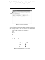
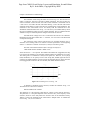
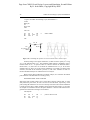
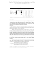
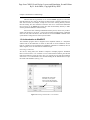
Page from CMOS Circuit Design, Layout, and Simulation, Second Edition
By R. Jacob Baker, Copyright Wiley-IEEE
Chapter 1 Introduction to CMOS Design
23
After the GDS file is generated, we can use the Gds2Tlc program to convert the
GDS file back into TLC files. In the setups we must specify a directory where the TLC
files will be written, for example, C:\temp. We can’t use a drawing directory because
then the existing TLC files would be overwritten. After we’ve converted the GDS back
into TLC files, we can Import the (scaled) TLC files into the dummy directory to make
sure the generated GDS file is scaled correctly.
Note, for the sake of feeling comfortable with this process, that it’s easy to take a
simple cell, like the test cell in Fig. 1.9 and convert it back and forth between a GDS file
and a TLC file (with scale factor). Also note that we can use the Resize command on the
system menu to change the size of the layout if needed.
1.3 An Introduction to WinSPICE
The simulation program with an integrated circuit emphasis (SPICE) is a ubiquitous
software tool for the simulation of circuits. In this book we’ll use WinSPICE. See the
links at cmosedu.com for download and installation information. WinSPICE, like all
SPICE engines, uses a text file netlist for simulation input.
Generating a Netlist File
We can use, among others, the Window’s notepad or wordpad programs. WinSPICE
likes to see files with a “*.cir” extension. To save a file with this extension, place the file
name and extension in quotes as seen in Fig. 1.22. If quotes are not used, then Windows
will tack on “.txt” to the filename. This can make finding the file difficult when we open
the netlist with WinSPICE (see Fig. 1.23).
Putting the file name with
extension (cir) in quotes
won't tack on the gratuitous
.txt to the end of the filename.
Figure 1.22 Saving a text file with a ".cir" extension.
Page from CMOS Circuit Design, Layout, and Simulation, Second Edition
By R. Jacob Baker, Copyright Wiley-IEEE
24
CMOS Circuit Design, Layout, and Simulation
Opening
a circuit
netlist.
Figure 1.23 Opening a file with WinSPICE.
Transient Analysis
A SPICE transient analysis simulates circuits in the time domain (like an oscilloscope the
x-axis is time). Let’s simulate the simple circuit seen in Fig. 1.24. A simulation netlist
(the text file) may look like:
*** Figure 1.25 CMOS: Circuit Design, Layout, and Simulation ***
.control
destroy all
run
plot vin vout
.endc
.tran 100p 100n
Vin
R1
R2
Vin
Vin
Vout
0
Vout
0
DC
1k
2k
1
.end
Vin
Vin, 1 V
R1, 1k
Vout
R2, 2k
Figure 1.24 Simulating the operation of a resistive divider.
Page from CMOS Circuit Design, Layout, and Simulation, Second Edition
By R. Jacob Baker, Copyright Wiley-IEEE
Chapter 1 Introduction to CMOS Design
25
The simulation results using this netlist are seen in Fig. 1.25. The first line in a
netlist is a title line. This line is ignored by SPICE (important). The next five lines are
control commands. Notice how the end of the control statement is terminated with an
“.endc” not an “.end” like at the end of the netlist. Placing “.end” at the end of the control
statement causes SPICE to ignore all of the lines containing the circuit information. The
statements in the control block can be run directly from the command line in the
WinSPICE command window seen in Fig. 1.23. The destroy all command destroys all of
the previous simulation results (so we don’t display old data). The run command runs the
simulation. The plot command plots the voltages on the nodes Vin and Vout.
Note that the DC voltage source Vin is connected to the node Vin. We could have
labeled the Vin node with a number like “1.” However, it is nice to have node names that
correspond with signals.
The connection of the resistors and how they are specified should be easy to
determine. A line starting with an “R” indicates a resistor specification. A line beginning
with an “*” indicates a comment. Node 0 (zero) is always reserved for ground.
The form of the transient statement (this is the type of analysis) is
.TRAN TSTEP TSTOP <TSTART> <TMAX> <UIC>
where the terms in < > are optional. The TSTEP term indicates the (suggested) time step
to be used in the simulation. The parameter TSTOP indicates the simulation’s stop time.
The starting time of a simulation is always time equals zero. However, for very large
(data) simulations, we can specify a time to start saving data, TSTART (again this term is
optional). The TMAX parameter is used to specify the maximum step size. If the plots start
to look jagged (like a sinewave that isn’t smooth), then TMAX should be reduced.
Vin
Vout
Figure 1.25 Simulating the circuit in Fig. 1.24.
To illustrate a simulation using a sinewave, examine the schematic in Fig. 1.26.
The statement for a sinewave in SPICE is
SIN VO VA FREQ <TD> <THETA>
The parameter VO is the sinusoid’s offset (the DC voltage in series with the sinewave).
The parameter VA is the peak amplitude of the sinewave. FREQ is the frequency of the
sinewave, while TD is the delay before the sinewave starts in the simulation. Finally,
THETA is used if the amplitude of the sinusoid has a damped nature. To simulate the
circuit in Fig. 1.26, we use a netlist of
Page from CMOS Circuit Design, Layout, and Simulation, Second Edition
By R. Jacob Baker, Copyright Wiley-IEEE
26
CMOS Circuit Design, Layout, and Simulation
*** Figure 1.26 CMOS: Circuit Design, Layout, and Simulation ***
.control
destroy all
run
plot vin vout
.endc
.tran 1n 3u
Vin
R1
R2
Vin
Vin
Vout
0
Vout
0
DC
1k
2k
0
SIN 0 1 1MEG
.end
Vin
R1, 1k
Vin
1V (peak) at
1 MHz
Vout
R2, 2k
Figure 1.26 Simulating the operation of a resistive divider with a sinewave input.
Some key things to note in this simulation: (1) MEG is used to specify 106. Using
“m” or “M” indicates milli or 103. The parameter 1MHz indicates 1 milliHertz. (Also, f
indicates femto or 1015. A capacitor value of 1f doesn’t indicate one farad but rather 1
femto Farad.) (2) Note how we increased the simulation time to 3 Ps. If we had a
simulation time of 100 ns (as in the previous simulation), we wouldn’t see much of the
sinewave (one-tenth of the sinewave’s period). (3) The “SIN” statement is used in a
transient simulation analysis. It is not used in an AC analysis.
Before leaving this introduction to transient analysis, let’s introduce the SPICE
pulse statement. This statement has a format given by
PULSE VINIT VFINAL TD TR TF PW PER
is the pulse’s initial voltage, VFINAL is the pulse’s final (or pulsed) value, TD is the
delay before the pulse starts, TR and TF are the rise and fall times, respectively, of the
pulse (noting that when these are set to zero the step size used in the transient simulation
is used); PW is the pulse’s width; and PER is the period of the pulse. Figure 1.27 provides
an example of a simulation that uses the pulse statement. A section of the netlist used to
generate the waveforms in this figure is seen below.
VINIT
.tran 100p 30n
Vin
R1
C1
Vin
Vin
Vout
0
Vout
0
DC
1k
1p
0
pulse 0 1 6n 0 0 3n 10n
Page from CMOS Circuit Design, Layout, and Simulation, Second Edition
By R. Jacob Baker, Copyright Wiley-IEEE
Chapter 1 Introduction to CMOS Design
Vin
0 to 1 V
delay 6ns
time at 1 V = 3 ns
period = 10 ns
R1, 1k
27
Vout
C1,
1p
Figure 1.27 Simulating the step response of an RC circuit using a pulsed source voltage.
Other Analysis
Besides the transient analysis presented in this section, we frequently use the SPICE DC
and AC analyses. The AC analysis has an x-axis of frequency. This type of analysis is the
common “small-signal” analysis used in a basic introductory microelectronics course.
The DC analysis has a DC voltage source for the x-axis. The value of the DC source is
swept while either a current of voltage is plotted on the y-axis. We don’t go into these
analyses here but provide numerous examples later in the book.
Convergence
A netlist that doesn’t simulate isn’t converging numerically. Assuming the circuit
contains no connection errors, there are basically three parameters that can be adjusted to
help convergence: ABSTOL, VNTOL, and RELTOL.
ABSTOL is the absolute current tolerance. Its default value is 1 pA. This means
that when a simulated circuit gets within 1 pA of its “actual” value, SPICE assumes that
the current has converged and moves onto the next time step or AC/DC value. VNTOL is
the node voltage tolerance, default value of 1 µV. RELTOL is the relative tolerance
parameter, default value of 0.001 (0.1 percent). RELTOL is used to avoid problems with
simulating large and small electrical values in the same circuit. For example, suppose the
default value of RELTOL and VNTOL were used in a simulation where the actual node
voltage is 1 V. The RELTOL parameter would signify an end to the simulation when the
node voltage was within 1 mV of 1 V (1V·RELTOL), while the VNTOL parameter
signifies an end when the node voltage is within 1 µV of 1 V. SPICE uses the larger of
the two, in this case the RELTOL parameter results, to signify that the node has
converged.
Increasing the value of these three parameters helps speed up the simulation and
assists with convergence problems at the price of reduced accuracy. To help with
convergence, the following statement can be added to a SPICE netlist:
.OPTIONS ABSTOL=1uA VNTOL=1mV RELTOL=0.01
To (hopefully) force convergence, these values can be increased to
.OPTIONS ABSTOL=1mA VNTOL=100mV RELTOL=0.1
Note that in some high-gain circuits with feedback (like the op-amp’s designed later in
the book) decreasing these values can actually help convergence.
Page from CMOS Circuit Design, Layout, and Simulation, Second Edition
By R. Jacob Baker, Copyright Wiley-IEEE
28
CMOS Circuit Design, Layout, and Simulation
Some Common Mistakes and Helpful Techniques
The following is a list helpful techniques for simulating circuits using SPICE.
1.
The first line in a SPICE netlist must be a comment line. SPICE ignores the first
line in a netlist file.
2.
One megaohm is specified using 1MEG, not 1M, 1m, or 1 MEG.
3.
One farad is specified by 1, not 1f or 1F. 1F means one femto-farad or 10–15
farads.
4.
Voltage source names should always be specified with a first letter of V. Current
source names should always start with an I.
5.
Transient simulations display time data; that is, the x-axis is time. A jagged plot
such as a sinewave that looks like a triangle wave or is simply not smooth is the
result of not specifying a maximum print step size.
6.
Convergence with a transient simulation can usually be helped by adding a UIC
(use initial conditions) to the end of a .tran statement.
7.
A simulation using MOSFETs must include the scale factor in a .options
statement unless the widths and lengths are specified with the actual (final) sizes.
8.
In general, the body connection of a PMOS device is connected to VDD, and the
body connection of an n-channel MOSFET is connected to ground. This is easily
checked in the SPICE netlist.
9.
Convergence in a DC sweep can often be helped by avoiding the power supply
boundaries. For example, sweeping a circuit from 0 to 1 V may not converge, but
sweeping from 0.05 to 0.95 will.
10.
In any simulation adding .OPTIONS RSHUNT=1E8 (or some other value of
resistor) can be used to help convergence. This statement adds a resistor in
parallel with every node in the circuit (see the WinSPICE manual for information
concerning the GMIN parameter). Using a value too small affects the simulation
results.
ADDITIONAL READING
[1]
D. E. Boyce, LASI User’s Manual, available while LASI is running by pressing
F1 on the keyboard and the button the user needs help with (at the same time).
Alternatively, the user can open the help file in the directory C:\Lasi7\help.
[2]
M. Smith, WinSPICE User’s Manual, Available for download (with the
WinSPICE simulation program) at http://www.winspice.co.uk/
PROBLEMS
In the following solutions, it can be very helpful to use the Prt Sc (print screen) button on
the keyboard to copy contents displayed on the computer’s display to the clip board. The
image of the display can then be pasted into a document. For ease of viewing (the
resulting pasted image in the document), it may also be useful reduce the display
resolution prior to using the Prt Sc button (right click on the desktop, select properties,
then settings).