Download Eavesdropper Tutorial - the Kansas Geological Survey

Eavesdropper
Tutorial
SEISMIC-REFLECTION PROCESSING DEMONSTRATION
USING EAVESDROPPER
by
Richard D. Miller
and
Don W. Steeples
KANSAS GEOLOGICAL SURVEY
1930 Constant Avenue
Lawrence, Kansas 66047-3726
Open-file Report #91-27
July 1991
TABLE OF CONTENTS
Page
I
CDP PROCESSING WITH EAVESDROPPER FOR THE NOVICE
A)
GENERAL CDP SEISMIC DATA PROCESSING FLOW
B)
TRACE HEADERS
C)
DATA FORMAT
D)
DISPLAY
E)
EDIT
1)
Manual bad-trace edit
2)
Automatic bad-trace edit
3)
First-arrival mute
4)
Surgical mute
F)
SORTING (GATHERING) INTO CDP FORMAT
G)
ELEVATION CORRECTION/DATUM ASSIGNMENT
H)
VELOCITY ANALYSIS
1)
Interactive velocity picking
2)
Constant velocity stack
3)
Time-spatial varying NMO
I)
SPECTRAL ANALYSIS
1)
Frequency vs amplitude
2)
Filtering
J)
AMPLITUDE BALANCING
1)
Automatic gain control (scale)
K)
STACK
1
1
4
6
8
11
12
18
20
24
28
45
51
52
55
61
65
65
69
76
76
79
II
FURTHER PROCESSING/ADVANCED TECHNIQUES
84
i
TABLE OF EXAMPLE DATA STEPS
Step No.
Introduction
1
2
3
3a
4
5
6
6a
6b
7
8
8a
8b
8c
9
9a
9b
10
10a
11
Operation
Data and format
Loading data on computer
Plotting raw field files
Bad trace editing
Manual editing procedure
First-arrival muting
Surgical muting
Stacking chart
Building sort deck
Data after sorting
Datum correction
Interactive velocity analysis
Constant velocity stacks
Picking appropriate velocity
Moved out field-file appearance
Spectral analysis
Reflection information
Batch processing file
Analysis of spectral plots
Application of AGC
CDP stacking of data
ii
Page
4
7
11
12
12
22
26
31
36
43
46
52
55
58
58
66
69
75
78
78
81
LIST OF FIGURES AND TABLES
Figure
1.
2.
3.
4.
5.
6.
7.
8.
9.
10.
11.
12.
13.
14.
15.
16.
17.
18.
19.
20.
Table 1.
Page
Raw field file SSN 5, England data.
Bad-trace edit file 5, England data.
Trace and taper.
First-arrival mute, file 5.
Surgical mute, file 5.
Page of field notebook.
Field notes for sample data set from England.
Stacking chart.
CDP sort of 245 and 146.
Constant velocity stacks (2).
Velocity function on file 5.
Spectra SSN 5, trace 18.
Spectra SSN 5, predominantly air wave.
Spectra SSN 5, predominantly ground roll.
Spectra SSN 5, predominantly refraction energy.
Spectra SSN 5, predominantly reflection energy.
Shape of the filter for 125 to 400 bandpass.
Filter of file 5.
Scale of file 5.
Brute stack of file 5.
13
17
21
25
29
32
33
34-35
44
59
60
68
70
71
72
73
74
77
80
83
Processing flow.
2-3
iii
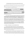
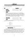
INSTALLATION INSTRUCTIONS:
Programs and data contained on the included disk will operate in a
fashion nearly identical to the full Eavesdropper package. The demonstration
software and manual have been compiled to instruct the novice as well as allow
a seasoned processor an opportunity to see and feel the flow of this seismicprocessing package. Only a small sampling of the operations available with the
Eavesdropper package are on this demo.
Four types of data are contained on the demonstration disk: 1) seismic
data (extension = *.raw or *.dat), 2) sample batch files (extension = *.dek), 3)
executable files (extension = *.exe), and 4) assistance files (extension = *.hlp or
*.cfg). The only files that can be displayed with the DOS type command are the
sample decks and set up files. To minimize confusion while processing this data,
it is advised that two sub-directories be created. The first sub-directory should
contain the executable files (extension *.exe) and should be named something
like eav. The second sub-directory should contain the sample batch files,
assistance file, and data files, and called something like demo. The path of your
computer will need to be modified so the executable files can be called on from
the demo directory. Once the files on the floppy disk have all been loaded into
the appropriate directory, you are ready to proceed through the manual.
iv
I. CDP PROCESSING WITH EAVESDROPPER FOR THE NOVICE
This document is designed to demonstrate the operation of Eavesdropper by providing stepby-step detailed instructions and explanations on seismic data processing from raw data to brute
stack.
NOTE: This document is separated into large type (representing processing steps) and smaller
type (indicative of explanation and background information).
The format of the text in this document was specifically designed to aid in identifying 1)
responses and information supplied to the user by the program upon request, 2) information or
commands supplied to the program, and 3) key points (highlights) to remember. The information
supplied by the program will be in italics and includes error messages, file contents displayed on
screen using the MS/DOS type command, messages concerning information being processed, notes to
the user concerning default parameters, etc. All italicized text in this manual indicates information generated by the program. Information you must supply to the program is always underlined
and in bold type and includes execution commands, parameters to input, spaces necessary, etc. Key
information to remember is always in bold type. After processing the sample data set completely
through using this manual, future data sets could be processed by referring only to the bold-type
information. You should become quite comfortable with the material in this manual after processing the sample reflection data set.
The Eavesdropper seismic data-processing package is divided into three main categories:
1) plotting and formatting, 2) filtering and deconvolution (FMAIN), and 3) the remainder of seismic
data processing (SEIS). The plotting and formatting operations are interactive requiring you to
execute the program and then enter the requested information. The filtering and deconvolution
routines are contained with the sub-program called FMAIN and are pseudo interactive. Processes in
FMAIN will ask a series of questions and then operate on the data set. The remainder of dataprocessing procedures are contained within the sub-program called SEIS. The program SEIS was
designed to operate in a batch processing mode, requiring an input job file and an output list file.
The input job file contains all the operation identifiers (*AUTS, *EDKL, *SORT, etc) along with
the appropriate user assigned parameters. The output list file contains all the significant steps and
processes completed during the executed batch job. The list file also contains bits of information
concerning processing time, any abnormalities in the flow, any error messages, etc. Operation of
Eavesdropper with the assistance of this manual requires a general knowledge of what seismic
reflection is as well as a working knowledge of your computer and the MS/DOS operating system.
(See information that came with your computer.)
A) GENERAL CDP SEISMIC DATA PROCESSING FLOW
The goal of digitally manipulating seismic data is to allow the maximum amount of
geologic information to be extracted from a minimal amount of data with a minimal amount of
effort. The processing of seismic data involves a series of steps. Each seismic processing step
generally has a prerequisite step or operation. This means a basic processing flow must be used to
effectively process seismic data. The exact processing flow you should use for your data set depends
mainly on two things: 1) the overall quality of your data and 2) the particular information you
intend to extract from the final processed section.
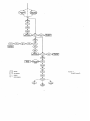
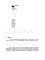
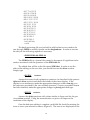
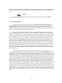
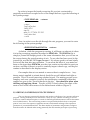
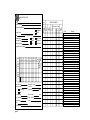
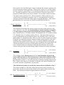
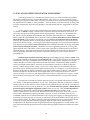
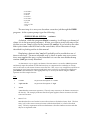
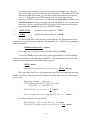
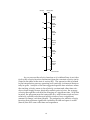
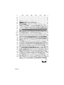
The processing flow we use is structured to maximize shallow high frequency CDP seismic
reflection data. The general outline of our processing flow is contained in table 1. Table 1 contains
all the operations we routinely use to go from raw field data to finished process sections. This
manual will discuss in some detail all the operations through brute stacking of seismic reflection
data. The intention of this novice user's manual is to get a person started and somewhat familiar
1
SEISMIC DATA PROCESSING FLOW CHART
cwck
L.
Screen Display
1 to Generate Hard Copy
4
Raw Formatted
Field Data
I
1
1
Bad Trace
Edited Data 4
I
l EDFM
4-G3--+-
Lr?*
Muted Data
El
Display
4-+GJ---
0
DispIay
*-
-0
r _
t-feque KY
Fitter #1
I
Pbt
--
-
Sorted Data-COP, Common Offset, Common Trace
Common Receiver, Common Shot
4
1Datum/Elevatbn
Corrected,
NMO”
Fun
’ . ’
.
+
Table #l of
Static Corfectbns
I
I
NM0 Ve&&y
Functh#2
6
Intermediate
Stack Section
l AUTS
NM0 Vehity
.
Function
#3
0
l FlLT #2
Table L
(contirmeg!l)
opefatiofl
data dewiption
sequence
optional sequence
0
i
with the organization as well as some of the rationale for key parameter selections. Each person
should establish a processing flow that is somewhat tailored to both the needs of the particular
survey and to existing equipment. Some operations can be reordered/removed/included/used
several times/etc., and will either enhance, deteriorate, or not change the final section; however,
some of the core operations (stacking, surface consistent statics, and normal moveout) do require prerequisite operations. All processing operations require proper formatting of the input data.
Processing seismic data requires a basic understanding of acoustic-wave propagation
through the earth (layered media). Attempting to process data without the necessary physics and
math background will eventually result in frustration or bogus results. To assist the novice/or outof-practice seismic data processor, a sample data set is included with this manual. The data were
collected during May, 1989, in England along the Thames River. Several good quality reflectors can
be interpreted directly off the raw field files. The data set will not present a significant challenge
for the seasoned seismic data processor, but it will require a variety of standard processing steps
properly applied to obtain a stacked section allowing the most realistic geologic interpretation.
INTRODUCTION TO
*********************EXAMPLE DATA*********************
The raw data include 20 field files chopped to 250 ms of record length at a
sample interval of 1/2 ms. The data were acquired with an EG&G 2401 seismograph (processing 24 channels), single 100-Hz geophones, a 12-gauge buffalo gun
(both the source and receiver intervals were 2.5 m), and 200 Hz analog low-cut
filters. Each step in the general processing flow followed in this manual will use
the England data set as the example. The field notes as well as the formatted data
are included with or within this manual.
B) TRACE HEADERS
Next to the data itself the trace headers are the most essential part of digital seismic
data. All acquisition information essential to future seismic data processing as well as to update
information derived from intermediate processing operations is organized and stored within each
trace header. The organization of trace headers is dependent only on the imagination of the programmer of the software and manufacturer of the seismograph. The particulars with respect to size
and organization of the trace header, its location with respect to the rest of the data set as well as
the organization and size of each sample of data within the trace itself is what is commonly referred to as seismic data format. The format of seismic data is critical to the effective operation of
seismic data processing programs. Imagine the resulting seismic section if the programmer of the
software designates a particular trace header location as the source station number and the seismograph manufacturer has designated that location as the receiver location.
A simple way to think of both the use and organization of a trace header is to compare it to
a business letter. A business letter will generally have two main parts, first is the letterhead and
second is the body of the letter. The critical part of the letter of course is the body. It contains the
significant information, the information that makes it different from any other letter. The
letterhead on the other hand is basically the same for every letter sent out by the business. The
only things that change within the letterhead are date and office of origin within the business.
The letterhead contains all the information necessary for someone to determine the business name,
section, address, and date of the letter. A seismic data trace (in digital form) can be thought of in a
4
similar way. The trace header serves a similar purpose as the letterhead. The data itself are
equivalent to the body of the letter.
Most, but not all, operations use the header to obtain key information about the data
contained within each trace. Some operations will update the header with information, others
will simply use the information to physically change the data set according to the prescribed
operation and designated parameters. The trace header locations will always remain the same.
The actual values within each word in the header can or will be changed in accordance with the
described operation and input parameters.
The standards for formats on seismographs have changed consistently through the years.
Such familiar acronyms as SEGA, SEGB, SEGY, modified SEGY, SEG2, etc. describe individual
variations. The recent advances into non-magnetic tape storage media have caused introduction of
a multitude of formats. For the most part, each manufacturer of a seismograph with non-9-track
tape-storage media has a preferred trace header format. A standardized format is being
considered. When a standard has been adopted, there will no longer be a need for the format
conversions described in a later section.
The key information necessary to process seismic data using Eavesdropper is contained
within the 240 byte (120-16 bit words) trace header preceding the seismic data itself which is
represented by 2 bytes per sample word (i.e., 500 sample/trace data represent a block of 1000 bytes).
Each header location is identified by a number (1-120). Eavesdropper expects to see a header at the
beginning of each trace (240 bytes) followed by a data block (length dependent on number of
samples). The header contains the following information at the designated word locations:
16-bit
Word Number
1
2
3
4
5
6
8
10
12
14
15
Description
Data type:
0 = Raw field files
1 = CDP gather
2 = CDP stacked
3 = Record order (Record number index and trace number index
based on values in trace header word 3 and 4, respectively).
4 = Velocity-scan data
Total recording channels
Trace Header Word of RECORD number for this data set where
8 = common recording channel number
12 = common depth point
19 = common offset
86 = common receiver station number
87 = common source station number
92 = common source sequence number
Trace Header Word of TRACE number within each record (0 = as input order of
seismic input data to be sorted).
Trace direction flag for sorted traces within each record — 1 = ascending
— 1 = descending
Original Field Record number
Recording channel number
Repeated shot number (at the same station)
CDP number
Trace number within each record
Trace identification code: 1 = seismic data
2 = dead
9 = velocity flag
5
16
17
19
21**
23**
27**
35
50*
51*
52*
55
58
59
70
71
75
76
82
83
84
85
86
87
88
89*
90*
92
93
94-120
*
Number of vertically summed traces yielding this trace
Number of horizontally summed traces yielding this trace
Offset (distance from source to receiver) after multiplied by word 35
Receiver group elevation
Source elevation
Datum elevation
Multiplication factor for horizontal distance
Source static correction (ms) (floating pt)
Receiver group static correction (ms) (floating pt)
Total static correction (ms) that HAS BEEN applied to this trace (zero if no
static has been applied).
Recording delay time (ms) (floating pt)
Number samples in this trace
Sample interval in micro-seconds for this trace
Analog low-cut frequency (Hz) (-3 dB pt)
Analog high-cut frequency (Hz) (-3 dB pt)
Applied digital low-cut frequency (Hz)
Applied digital high-cut frequency (Hz)
Minimum receiver station number
Maximum receiver station number
Minimum source sequence number
Maximum source sequence number
Receiver station number for this trace
Source station number for this trace
Last trace flag: 0 = not last trace; 1 = last trace
Surface-consistent residual receiver-static (in number of SAMPLES) that HAS
BEEN applied to this trace.
Surface-consistent residual source-static (in number of SAMPLES) that HAS
BEEN applied to this trace.
Source sequence number
Processing history file flag: 0 = No history; non-zero = number of characters in
file name to follow.
Reserved for processing history file name. Packed ASCII. Two ASCII
characters per word.
Convention for static corrections: POSITIVE value implies static shift (DOWN) away from
zero-time; NEGATIVE value implies static shift (UP) toward zero-time.
* * Elevation can be either absolute (i.e., positively above sea level) or relative (with reference to
fixed altitude). In both cases, the orientation is such that higher elevation is positive.
Therefore, increasing depth is indicated by the smaller value for elevation.
Note: ms = milliseconds
C) DATA FORMAT
Formatting of seismic-reflection data involves organizing trace headers and data bytes into
a specific pattern and sequence recognizable by Eavesdropper. The formatting utilities available
for Eavesdropper require raw unformatted data to be present on hard disk. The formatting utilities
(conversion routines) are designed to operate on raw data input from hard disk and output back to
hard disk. Getting the raw data from the seismograph's preferred storage media (floppy disk, 9
track tape, tape cartridge, RAM, etc.) onto the hard disk requires procedures, software, and/or
6
hardware that can be supplied by the seismograph manufacturer. Often the transfer of raw unformatted data to a computer's hard disk requires nothing more than the MS/DOS copy command.
The particular formatting routine necessary for your raw unformatted data depends on the
seismograph with which it was collected. Until a standardized format can be established and
agreed upon by all seismograph manufacturers and software developers, a different conversion
routine will be necessary for most new and existing seismographs. At the time of this writing,
Eavesdropper facilitates the following data formats:
Program
90002KGS
BISCONV
EASI2KGS
SEGI2KGS
SEGF2KGS
SEGPFKGS
SV2KGS
GEOF2KGS
24012KGS
DFSDEMUX
SEG22KGS
ABEM2KGS
DG2KGS
DHR2KGS
SCIN2KGS
Description
9000(Bison) to KGS
Geopro(Bison) to KGS
EASIDISK (EG&G seismograph) to KGS
SEGYinteger to KGS
*SEGYfloatingpoint to KGS
**SEGYfloatingpoint to KGS
Seisview(EG&G) to KGS
GeoFlex(EG&G) to KGS
2401(EG&G) to KGS
***SEGBdemuliplex to KGS
SEG 2 engineering format to KGS
ABEM seismograph to KGS
Data General to KGS
I/O DHR 2400 to KGS
Scintrex seismograph to KGS
* 1) VAX/ MAINFRAME
** 2) IEEE/ IBM-PC
*** Available as separate package.
Raw unformatted data on your hard disk will be in the form of a sequence of files with
identical prefixes and/or extensions, where each file represents a unique field file recorded on your
seismograph and downloaded onto your computer's hard disk. The naming process was done during
either the downloading of your data to your computer's hard disk or at the time of acquisition and
storage of the data in the field. The total number of these individual sequential files will be equal
to the number of field files copied onto your hard disk. Once the data are on the hard disk of your
computer (in most cases this involves a simple copy command), the appropriate conversion routine
should be executed to correctly format your data for future processing with Eavesdropper software.
After completing the formatting operation, all the individual field files should be contained in a
single MS/DOS file.
STEP #1
**********************EXAMPLE DATA********************
Copy the contents of the floppy onto your hard disk. When you list the
directory as below, the following sequence of files should be present on your hard
disk:
7
>dir <return>
dplot.exe
dseis.exe
dview.exe
dengland.dat
dvscn.exe
dfmain.exe
dvelp.exe
fmain.hlp
view.cfg
plot.cfg
nmot.dek
scal.dek
edfm.dek
edkl.dek
rsrt.dek
filt.dek
process.dek
edmt.dek
sort.dek
stak.dek
surf.dek
The extension (*.ext) can be used for quick and easy identification of filetype. For example, files referred to in this document with an *.exe extension are
executable codes, *.cfg extensions are graphics configuration files, *.dat are
seismic data files, *.dek are batch processing command files, and *.1st are journal
or list files.
D) DISPLAY
Eavesdropper can display seismic data either variable-area wiggle-trace or just wiggletrace on your CGA, EGA, or VGA CRT with a hardcopy print option. Two routines are contained
within Eavesdropper to display data. The dview routine is mainly designed as a quick way to see
data on the CRT without a hardcopy option. This quick display routine is most helpful during
preliminary plot parameter design. The main plotting routine is called dplot. Dplot prepares and
displays the data on the CRT with a hardcopy option. During your first attempts at plotting, we
recommend using dview to select the appropriate plotting parameters, followed by dplot for final
CRT display and hardcopy.
After your data are in Eavesdropper format, examination of a variable area wiggle-trace
display of all the unprocessed data will allow you to verify proper formatting as well as to get a
general feel for the quality and quantity of data. The processes involved with getting a display
using either dplot or dview will be discussed simultaneously. This should cause no confusion since
dview and dplot generate exactly the same output. The dview routine has no hardcopy option and,
therefore, the screen display in dview is several times faster than dplot. The few minor differences
in requested parameters that occur will be discussed at the appropriate time.
8
To set the basic plotting parameters, you will need to edit the plot.cfg (plot configuration)
or view.cfg (view configuration) file. NOTE: both *.cfg files are in the EAV subdirectory and can
only be altered from that subdirectory. Enter your text editor and open either the plot.cfg.or the
view.cfg file.
The view.cfg TEXT FILE will have 7 lines, with each line requiring a particular parameter,
as indicated below:
Line
Default Value
1
2
3
0
350
50
4
65
5
0
6
0
7
100
8
2
Description
This is a dummy line not used by the dview routine.
Designates the number of pixels on the EGA screen.
Approximate vertical resolution for the EGA monitor (13").
(DOTS/INCH)
Approximate horizontal resolution for the EGA monitor (13").
(DOTS/INCH)
Whole trace gain applied in dB. This value can be either
negative or positive.
Designates either variable area wiggle-trace (0) or just wiggletrace (1) display format.
Tells dview what percentage of the allotted trace spacing the
trace may occupy. For example, assume that the trace spacing is
10 per inch. Each trace has an allotted area of .1". If line 7 is
100 percent, the trace may 'wiggle' as much as .1". If line 7 is,
say 200 percent, then the trace 'wiggle' may be as wide as .2".
Values of 150 to 200 generally give pleasing results.
GAP between field records.
The plot.cfg file has strong similarities to view.cfg. The text file you just opened has 8 lines
each with its associated default value.
Line
Default Value
1
2
3
0
0
120
4
144
5
0
6
7
0
100
8
2
Description
density 1=high density; 0=low density. Default is 0.
dots/line on the attached printer; generally either 960 or 1632.
Vertical resolution [dots/inch on the vertical scale (time)]; full
scale on standard printers is 120.
Horizontal resolution [dots/inch on horizontal scale (distance)];
full scale on standard printers is 144.
This parameter controls the application of a constant gain (in
decibels) to the data before plotting.
dplot style 0=variable area wiggle-trace; 1=wiggle-trace.
Tells dplot what percentage of the allotted trace spacing the
trace may occupy. For example, assume that the trace spacing
is 10 per inch. Each trace has an allotted area of .1". If line 7
is 100 percent, the trace may 'wiggle' as much as .1". If line 7
is, say 200 percent, then the trace 'wiggle' may be as wide as .2
Inch. Values of 150 to 200 generally give pleasing results.
Controls the number of blank traces inserted between field records.
After editing plot.cfg and/or view.cfg, return to your working directory, and at the system
prompt execute whichever display routine you desire.
9
> dview
<return>
or
> dplot
<return>
The first question the plot or view program will ask is:
("enter filename to plot"). dengland.raw
After you have entered the file name (dengland.raw), the program will respond with one or
more of the following statements:
1) "No processing history file available" which means basically that no processing has
been completed at this point, so the file designed to handle the processing history has not
been created yet,
2) "Processing history file name found" which means basically what it says, and the result
will be the printing of the current processing history at the conclusion of the plotting of the
data.
3) "Warning—History file—FNAME.HO1—not found" meaning that there should be a
history file called FNAME present from previous processing, but dplot was unable to find it.
4) "Plot.cfg not found" which means it was not able to find the plot.cfg file, and the
predesignated default parameters will be used.
In the case of raw data such as we are displaying at this time, the program should respond
with statement (1), only. This is assuming plot.cfg or view.cfg, depending on the requested routine,
is present and has been updated according to the previous instructions.
If at any time you wish to return to the system prompt hit 'Crtl C ' —
Enter starting record number (default=first record found for data set) ->
Enter ending record number (default=32000) ->
*Do you want auto screen dump? 0=No/1=Yes (default=0) ->
Enter vertical display size in inches/second (default=data dependent) ->
Plot normal ? 0=off 1=on (default=0) ->
**Enter normalize scan delay in ms (default=0) ->
Enter starting time of plot in ms (0) ->
Enter trace spacing in trace/inch (default=data dependent)
(values over 24 degrade hardcopy) ->
* Only applies to dplot program
** Only an option when plot normalization is selected
NOTE: data-dependent means program calculates a value it considers to be optimum for the input
data set.
10
NOTE: If at any time you wish to terminate the plotting process, press the space bar.
The plot normal option increases the amplitude of each individual trace by multiplying
each sample by a normalization constant, independent of all other traces in the data set. The
amount of this whole trace amplitude increase can be different for each trace and is related to the
difference between the largest amplitude sample in the trace and the maximum possible amplitude
that can be displayed.
The normalize scan delay time designates the beginning of the amplitude scan window used
to determine the multiplication factor for all the samples within the trace. The utility of this
option can be appreciated on data sets with abnormally high amplitude first-arrival information.
Selecting the beginning scan time after a large amplitude event allows events later in time to
dictate the amount of uniform whole trace amplification applied.
This program is FIELD-SENSITIVE, which means, don't put spaces after a prompt and/or
before the requested information unless directed by the program.
Both dplot and dview routines will return system control after the display process is
complete.
STEP #2
*********************EXAMPLE DATA*********************
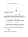
A hard copy plot of the raw England field data should contain 20 files
identified by the source sequence number in the upper right hand corner of each
file. The data were collected on a 24-channel seismograph. Therefore, there will
be 24 individual traces within each field file. The traces within each field file are
identified by original channel numbers starting with channel 1 on the left-hand
side of the field file, and channel 24 on the far right.
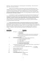
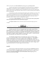
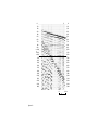
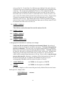
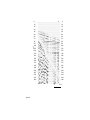
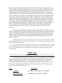
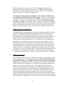
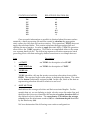
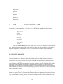
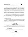
The field file displayed here has all the major types of seismic energy
arrivals you will encounter on most seismic data sets (Figure 1). Identified on
the plot of field file 5 is each trace number, time in milliseconds, refraction
energy, air-coupled waves, ground roll, and of course reflection events. Of interest for later processing steps, two dead traces are identified at trace numbers 8 and
23. The field file displayed has been scaled to enhance the seismic energy, making the identification of various types of arrivals easier.
E) EDIT
The next step in a standard processing flow involves the removal of bad traces (generally
caused by dead geophones, bad geophone plants, seismograph amplifier failure, cultural noise, or
poor near-surface conditions), bad parts of traces (generally results from the air-coupled wave or
ground roll), and energy arriving prior to the first identifiable reflection signal (generally
refraction and direct-wave energy).
11
1) Manual Bad-Trace Edit
Removal of dead or bad traces is the first editing step. This can be accomplished in two
different ways. The first way (the more standard technique) involves the manual entering of each
trace (to be removed) into a text-editor built edit deck using the *EDKL procedure. The second way
uses an automatic whole trace-editing routine *AUED procedure designed to identify (and automatically remove if specified) any trace that doesn't meet the minimum operator-specified signalto-noise ratio (S/N). In order to develop a good working knowledge of what and how the editing
process works, it is recommended that command of the manual editing technique be established
prior to extensive use of the automatic editing option.
STEP #3
*********************EXAMPLE DATA*********************
A plot of the raw-field data is critical at this step. Careful examination of
each trace of every field file will allow you to determine how much and what
type of editing will be necessary. The object of this stage is to remove all traces
and parts of traces with an unacceptable signal-to-noise ratio (S/N).
Determination of useless traces is subjective and your ability to make that
determination will drastically improve with experience. Traces 8 and 23 of the
displayed source sequence file 5 (Figure 1) are bad traces. It is important to
remember (all things being equal), that 2- or 3-fold of high-quality reflection data
are better than 48-fold of garbage data. The confidence necessary to effectively
edit will come with time and exposure to a variety of data sets.
STEP #3a
*********************EXAMPLE DATA*********************
The manual editing procedure is a batch-processing operation and
therefore requires a batch-processing file constructed around the *EDKL
identification. In order to build a batch-processing file you must use your TEXT
EDITOR. NOTE: Any text editor that does not leave embedded commands will
work (i.e., EDLIN, SIDEKICK NOTEPAD, XTREE, etc.).
This is the first batch processing deck described in this manual; therefore,
each part will be discussed in some detail and referred to during upcoming
processes.
Line
1
Description
>>START
start simply identifies the beginning of this processing deck.
2
*INPF dengland.raw
12
trace numbers
0
file
number
dead
traces
5
1 2 3 4 5 6 etc.
0
10
20
10
30
40
30 refraction
40
50
60
50
60
70
ground
80
roll
90
70
20
80
100
m100
s
e 110
c 120
110
120
140
130
140
150
150
160
160
170
170
180
180
190
190
200
200
210
220
220
230
230
240
240
130
210
0
figure 1
reflections
90
12 m
aircoupled
wave
*INPF identifies the input files. The alpha character name of the input
file, including any extension must follow *inpf, leaving at least one space
separating the f in *inpf and the first character of the file name.
Entries following an alpha identifier (i.e., *INPF, *EDKL, *AUTS,) need
only be separated by a minimum of one space. In other words, during
batch processing, any input information need only be in the correct
relative sequence. The program dseis is insensitive to absolute field
location and small or large case (i.e., A or a).
3
*EDKL 92 8
EDKL calls the "kill trace" sub-routine. The traces to be removed are
identified by a record-number trace-number pair [92 (SSN), 8 (field-trace
number)].
Record numbers generally identify the primary grouping order. In case of
raw field data, the primary grouping is by field-file number which is contained in trace-header location 6; for CDP gathers, the primary grouping is
according to CDP number which is contained in trace-header location 12.
Trace numbers generally identify secondary grouping order. In the case of
raw field files, the secondary grouping is according to seismograph
channel numbers which is contained in trace-header word 8. This grouping or ordering can be changed during the sorting or re-sorting operation.
These record/trace pairs can be thought of in a similar fashion to cards in a
deck of playing cards; that is, the suite (hearts, clubs, spades, diamonds) can
be thought of as the record number and the value (Queen, Jack, ten, nine,
etc.) can be compared to the trace number, such that any trace can be
identified by record number and trace number in the same fashion any
playing card can be identified by suite and value.
The program allows you to select any trace-header word to be the record
number portion as well as any trace header word for the trace number
portion of the record-trace pair. In this case, we wish to use Source
Sequence Numbers (SSN) (assigned during formatting), header word 92, as
the record number portion and the trace numbers within each field record,
header word 8, (which is the seismograph's actual channel numbers) as
the trace number. (Assigned by seismograph during acquisition)
4
KILL 1 1 12 12
KILL is a command operation that identifies which trace(s) within the
specified records are to be removed. In the above case, trace 12 record
number 1, will be removed.
14
5
KILL 2 2 11 11
KILL 3 3 10 10
KILL 4 4 9 9 24 24
Traces 9 and 24 of record 4 will be removed.
KILL 5 5 8 8 23 23
KILL 6 6 7 7 22 22
KILL 7 7 6 6 21 21
KILL 8 8 5 5 20 20
KILL 9 9 4 4 19 19
KILL 10 10 3 3 18 18
KILL 11 11 2 2 17 17
KILL 12 12 1 1 16 16
KILL 13 13 15 15
KILL 14 14 14 14
KILL 15 15 13 13
KILL 16 16 12 12
KILL 17 17 11 11
KILL 18 18 10 10
KILL 19 19 9 9
KILL 20 20 9 9
6
*OUTF EdKL.dat
*OUTF identifies the destination file name of the edited data. The file
name can be any MS/DOS acceptable name with or without extension.
The output file name can be the same as the input. Of course, if the input
file name is the output file name, the input data will be deleted and
replaced with the edited output data.
7
>>END
>>END identifies the last line of this batch-processing deck.
The actual bad trace edit file just created will look like the following:
>>start
*inpf dengland.raw
*edkl 92 8
kill 1 1 12 12
kill 2 2 11 11
kill 3 3 10 10
kill 4 4 9 9 24 24
kill 5 5 8 8 23 23
kill 6 6 7 7 22 22
15
kill 7 7 6 6 21 21
kill 8 8 5 5 20 20
kill 9 9 4 4 19 19
kill 10 10 3 3 18 18
kill 11 11 2 2 17 17
kill 12 12 1 1 16 16
kill 13 13 15 15
kill 14 14 14 14
kill 15 15 13 13
kill 16 16 12 12
kill 17 17 11 11
kill 18 18 10 10
kill 19 19 9 9
kill 20 20 9 9
*outf edkl.dat
>>end
The batch processing file you just built to edit bad traces now needs to be
run through DSEIS to actually operate on the dengland.raw. In order to execute
the edit job, the following sequence is necessary:
>DSEIS EDKL.dek EDKL.lst
The EDKL.lst file is a journal file created to document all significant information associated with the operation of the EDKL.dek file.
The edited data will be in the file named EDKL.dat. In order to see the
effect of the editing on the raw data, you should first use the dview routine.
Simply type:
>DVIEW
<return>
Answer the series of self-explanatory questions (as described in the preious
dplot and dview section) and check the format of the screen display. If the
display is not satisfactory, make the appropriate changes to either view.cfg or to
the responses provided to the view routine questions. Once an acceptable format
has been obtained, make the appropriate changes to plot.cfg and then type:
>DPLOT
<return>
Answer the dplot questions with values similar to those used for the previous dview routine. Using the normalization on plots will improve the
usefulness of the display.
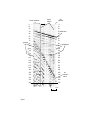
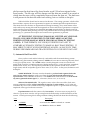
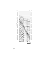
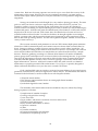
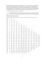
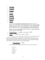
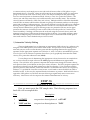
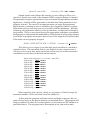
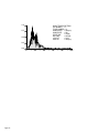
Once the bad-trace editing is complete, each field file should be missing the
trace or traces you selected to remove (Figure 2). The trace is not displayed on the
16
5
0
10
10
20
20
30
30
40
40
50
60
50
60
70
70
80
80
90
90
m100
100
s
e 110
c 120
120
130
140
130
140
150
150
160
160
170
170
180
180
190
190
200
200
210
210
220
220
230
230
240
240
110
0
figure 2
0
12 m
plot because the dead-trace flag (trace header word 15) has been tripped in the
trace header. The file size will not change until the data are sorted or re-sorted at
which time the trace will be completely removed from the data set. The bad trace
is still present in the data file after trace editing, but not visible on the plot.
Whole field files should not be removed at this time. The sorting operation, which will be
discussed later, requires all source geometries be input in an uninterrupted file sequential format.
This means that once the data are sequentialized (during formatting) , they must remain in that
order without any missing files until the assignment of source-and-receiver geometries is complete.
At the time the source geometries are identified (sn or snsn), entire bad files can then be removed.
This is not a problem when plucking out only a few particular files from a large data set if no future
processing (i.e., operations that require source-and-receiver geometries) is planned.
AT THIS POINT, IF YOU HAVE MANUALLY EDITED ALL YOUR BAD
TRACES, YOU SHOULD PROCEED TO THE FIRST-ARRIVAL MUTING
PORTION OF THIS MANUAL WHICH FOLLOWS AUTOMATIC EDITING
(*AUED). IF TIME PERMITS, USE YOUR JUST-EDITED DATA SET TO
COMPARE AUTOMATIC EDITING TO MANUAL BAD TRACE EDITING. IT
MAY SERVE TO HELP YOUR CONFIDENCE AS WELL AS SAVE YOU TIME
DURING PRELIMINARY BAD TRACE EDITING ON YOUR NEXT DATA SET.
2) Automatic Bad-Trace Edit
Once you have used and feel relatively comfortable with the manual editing routine
(*EDKL), using the automatic editing routine (*AUED) will save time in removing obviously dead
or very poor-quality traces. The *AUED routine is mainly designed to remove traces that are
totally dead or possess a significant amount of background noise (i.e., wind, powerline, automobile,
human traffic on line, etc.). The important parameters in this operation are the noise window
length (time) and the acceptable signal-to-noise ratio (S/N) value. At this point, definitions will
be helpful.
NOISE WINDOW: The noise window identifies a pre-first-break segment (before the
arrival of any seismic signal) on each trace where the level of background ambient noise is
representative of the remainder of the trace. The window needs to be selected so as not to include
any source generated seismic signal (i.e., refractions, direct wave, or air wave).
SIGNAL-TO-NOISE (S/N): The signal-to-noise value is the ratio of the whole trace
average amplitude and the average amplitude of signal in the noise window. A S/N value of 1
will retain any trace with a whole trace average amplitude equal to or greater than the average
amplitude of the signal in the noise window.
Experimentation with this routine is the best teacher. A few test runs varying the S/N
value for a given noise window will give insight into both the utility and the limitations of this
routine. A batch-processing file for doing automatic editing should look about like the following:
Line
Description
1
>> START
see manual edit *EDKL for details on >>start.
2
*INPF dengland.raw
see *EDKL for details on *INPF.
18
3
*AUED 20 0.28 1 1 1
*AUED calls the auto-edit sub-routine. The first requested parameter is the noise window.
Here 20 ms is used, indicating that no source-generated signal arrives on any trace before 20
ms. The second requested parameter is the signal-to-noise ratio (S/N) value. A signal-tonoise ratio of 0.28 means any trace not possessing an average whole-trace amplitude at least
0.28 times the average pre-first-break amplitude will be flagged. The third requested
parameter instructs the program to print (1) or not to print (0) the calculated average whole
trace signal-to-noise ratios (S/N) in the list file. The fourth requested parameter instructs
the program to print (1) or not to print (0) the flagged bad traces in the list file. This fourth
option gives you the opportunity to examine the traces the program suspects as being bad.
The fifth and final option lets you delete the flagged bad traces (1) or save all the traces as
inputted (0). This allows examination of the suggested bad traces and readjustment of
parameter 1 (noise window) and 2 (signal-to-noise ratio), or both. If the 0 option is chosen
for the fifth parameter, no output file need be named.
4
*OUTF Aued.dat
see *EDKL for details on *OUTF.
5
>>end
see *EDKL for details on >>end
The batch-processing file AUED.DEK you just saved looks like the following:
>>start
*inpf dengland.raw
*aued 20 0.28 1 1 1
*outf Aued.dat
>>end
In order to execute the automatic editing operation on the raw input data, the following
sequence again will be necessary:
>DSEIS AUED.DEK AUED.LST
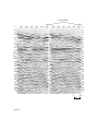
The AUED.LST file monitors and records the sequence of processing events.
The following information is included to allow you to check the contents of your list file
with what should be there:
List of example of signal-to-noise ratio of SSN 4:
4:
3.24
0.32
2.43
0.94
3.39
0.44
3.10
0.92
5.60
2.45
3.26
1.26
0.62
1.42
1.45
0.64
0.23
2.11
1.42
1.14
0.81
0.71
1.47
0.21
List of bad traces for SSN 4 from automated editing:
4:
9 24
The edited data will be in the file named AUED.dat. In order to see the effect of the
editing on the raw data, you should first use the dview routine. Simply type:
> DVIEW
<return>
Answer the series of self-explanatory questions (as described in the display section of this
manual) and check the format of the screen display. If the display is not satisfactory, make the
19
appropriate changes to either view.cfg or to the responses provided to the view routine questions.
Once an acceptable format has been obtained, make the appropriate changes to plot.cfg and then
type:
> DPLOT
<return>
Answer the dplot questions with values similar to those used for the previous dview
routine.
3) First-Arrival Mute
The next step in the processing flow involves the muting of refracted and direct-wave
energy (*EDFM). This is necessary on most data sets to ensure that refracted and/or direct-wave
energy does not appear coherent on CDP stacked sections. The high amplitude as well as the
coherent nature of moved-out and stacked refraction energy is inviting, and in some situations it can
easily be misinterpreted as shallow-reflection energy.
Complete identification of refracted energy is sometimes difficult on CDP stacked data.
Refraction energy has theoretically linear moveout on field files. The NMO velocity correction
applied to compensate for non-vertically incident reflection energy is hyperbolic. When refraction
wavelets, generally non-minimum phase and rarely broad band, are NMO corrected and stacked,
they can misalign in such a way as to appear as multiple, broad band, coherent reflection events
very dissimilar from the original refraction wavelets on the raw-field data. The appearance of
refraction energy on CDP-stacked data can many times entice the creative interpreter and/or geocontractor into a fatal pitfall. Unmuted refracted energy from a subsurface layer that varies in
depth, can appear to be a structurally significant, coherent reflection event on CDP stacked data.
This illusion on stacked data results from the changes in the critical refraction distance and time
intercept as the depth to the refracting interface varies. This pitfall many go unnoticed on some
data sets, since in some geologic conditions stacked refractions many be representative, in a gross
sense, of actual shallow structure. Such stacked refractions typically have lower frequency than
shallow reflections.
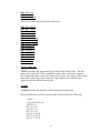
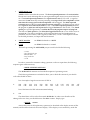
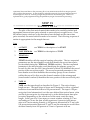
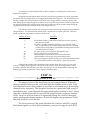
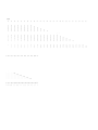
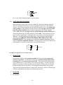
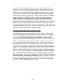
Any editing operation that requires the defining of a time window or beginning and/or
ending points for the zeroing of data will require the defining of a taper length (TAPR). The taper
is intended to allow the gradual attenuation of the trace amplitudes to zero without generating an
abrupt truncation point and the associated apparent high frequencies. If the trace is filtered at any
time in the processing flow without a taper, the abrupt truncation of signal resulting from a mute
will produce a complex sine function with maximum amplitude at the truncation point decaying to
near zero within the muted zone. The frequency and decay length of the sinusoid is dependent on
the defined filter. This decaying sinusoid is an artifact of the Fast Fourier Transformation (FFT)
which is part of the spectral filtering process. Frequency filtering is often necessary to remove or
attenuate unwanted noise. Choosing a taper length is a very data-dependent undertaking. At least
one cycle of the dominant-reflection frequency or center frequency of the digital band-pass filter
designed for this data set is a good starting point for defining a taper length. Fine tuning of a mute
taper generally is not necessary, but in certain instances returning to this step in the processing flow
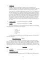
to better define a taper length may be necessary. During future processing operations involving a
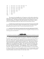
taper, reference to this paragraph will be made. In Eavesdropper, the taper is defined according to
Figure 3.
20
Original Trace
Surgical Mute Taper
First Arrival Mute Taper
taper
length
(ms)
defined
beginning
time
defined
ending
time
taper
length
(ms)
-1
0
1
relative amplitude
figure 3
-1
0
1
relative amplitude
defined
time
taper
length
(ms)
-1
0
1
relative amplitude
STEP #4
*********************EXAMPLE DATA*********************
The first step in the first-arrival muting process is to identify refracted and
direct-wave energy on your raw-field plots (Figure 1). Once a definite identification is made, the appropriate mute can be designed. Once the mute window for
each field file has been determined, a batch processing sequence similar to the
following should be created.
Line
Description
1
>>START
see *EDKL for description of >>START
2
*INPF EDKL.dat
see *EDKL for description of *INPF
3
*EDFM 92 8
*EDFM identifier calls the first-arrival mute subroutine. The two
requested parameters are trace-header words that identify the record/trace
pairs (as described during the *EDKL routine). The first requested parameter identifies the primary groups or records (in this case the SSN's traceheader location 92 identifies the record portion of the record-trace pair).
The second requested parameter is the trace-header word that identifies
the secondary groups or traces location within the record (in this case the
channel numbers of the seismograph, trace-header location 8, identifies
the trace portion of the record-trace pair).
4
TAPR 10
tapr sets the taper length. The length is in ms. The taper slope is linear
and is designed to allow a gradual transition from unaffected data to 100
percent mute. The taper's 0 percent point (total attenuation) is at the userdefined first-arrival mute value and the 100 percent point (no attenuation)
is at the defined mute time plus the taper length. In this case, if the firstarrival mute extended to 30 ms on trace 1, the taper would attenuate 90
percent of the signal at 31 ms, 80 percent of the signal at 32 ms, 70 percent
of the signal at 33 ms, etc. until at 39 ms 10 percent of the signal was
attenuated.
5a FARM 1 1 30 2 32 3 33 4 35 5 36 6 38 7 39 8 41 9 42 10 44 11 45 12 47 13 48 14 50
15 51 16 53 17 54 18 56 19 57 20 59 21 60 22 62 23 63 24 65
FARM defines first arrival mute times according to SSN and trace number. The farm operation is designed to interpolate both in time and space.
This interpolation process makes the entry on line 5b the same as the
22
entry on line 5a. If only line 5a or 5b farm was defined, the entire data set
would be first-arrival muted according to the defined record number-time
windows. The actual mute defined by line 5a or 5b would include the
entire data set and delete all data between time zero and 30 ms on trace 1,
from time zero to 32 ms on trace 2, from time zero to 33 ms on trace 3, etc.
out to trace 24 which will be muted from time zero to 65 ms. If more than
24 traces are present in this data set, each trace beyond trace 24 will be
muted as trace 24 was. This means that trace 25 will be muted from time
zero to 65 ms, trace 26 will be muted from time zero to 65 ms, trace 27 will
be muted from time zero to 65 ms, etc.
5b FARM 1 1 30 24 65
This defines exactly the same first-arrival mute as line 5a.
† 6a
FARM 2 1 0 24 0
† 6b FARM 3 1 30 24 65
† 6c
FARM 4 1 0 24 0
† 6d FARM 3 1 30 24 65 25 0
† Not appropriate for this data set—used only as an example .
If only one file of several is to be first-arrival muted (farm), the series of
entries on lines 6a, 6b and 6c would be necessary. The linear interpolation
process is automatic. The only way to stop the interpolation is to define 0
mute times just before and just after the defined mutes. The farm defined
by lines 6a, 6b, and 6c will mute file (SSN) 3 only, with trace 1 muted from
time zero to 30 ms trace 2 from time zero to 32 ms, etc. out to trace 24,
which will be muted from time zero to 45 ms If you wish to stop the mute
process after trace 24 , therefore, retaining all the information in traces 25
to the last trace (48, 96, or whatever the number of traces on your
seismograph), line 6d would be entered in place of line 6b.
7
*OUTF EDFM.dat
see *EDKL for description of *OUTF
8
>>END
see *EDKL for description of >>END
In order to display on the screen the previously defined first-arrival mute
batch process, simply enter:
>TYPE EDFM.dek
<return>
>>start
23
*inpf edkl.dat
*edfm 92 8
tapr 10
farm 1 1 30 24 65
*outf edfm.dat
>>end
Now, to run the previously defined first-arrival mute, you need to type
the following:
>DSEIS EDFM.dek EDFM.LST
As before, EDFM.LST is simply a journal file. The muted data will be in
the file named EDFM.dat. In order to see the effect of your mute on the input
data EDKL.dat, you need to use the dview routine. Simply type:
>DVIEW
<return>
Answer the series of self-explanatory questions (as described in display
section) and check the format of the screen display. If the display is not satisfactory, make the appropriate changes to either view.cfg or to the responses provided to the view routine questions. Once an acceptable format has been
obtained, make the appropriate changes to plot.cfg and then type:
>DPLOT
<return>
and answer the questions in a similar fashion as you view responses that
resulted in the appropriate display.
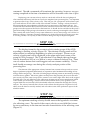
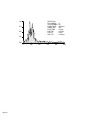
The first-arrival mute defined by the previous batch file will result in a
mute on all files of the sample data set. First-arrival information on file 5 will
begin at 30 ms on trace 1 and 65 ms on trace 24 with a 10 ms taper (Figure 4). This
field file is displayed identical to the file in Figures 1 and 2 allowing direct
comparison of before and after.
4) Surgical Mute
The final editing step involves the surgical removal of bad trace segments (*EDMT).
Noises resulting from the air-coupled wave, electronic interference other than power line frequencies, and ground roll are generally constrained to isolated portions of a trace. High-amplitude noise
obviously dominating a well-defined time window should be removed. However, care need be
taken when removing these low S/N portions of traces since significant seismic signal could be present on unprocessed data at an amplitude level below the dynamic range of the plot and therefore
invisible to the eye. If the amplitude of the unwanted noise is low in comparison to signal at equivalent times on other traces, occasionally the multi-trace stacking process necessary to generate a
CDP stacked section will suppress noise to an acceptable level. Also, many times various filtering
24
5
0
10
10
20
20
30
30
40
40
50
60
50
60
70
70
80
80
90
90
m100
100
s
e 110
c 120
120
130
140
130
140
150
150
160
160
170
170
180
180
190
190
200
200
210
210
220
220
230
230
240
240
110
0
figure 4
0
12 m
operations (discussed later in the processing flow) can attenuate noise that has unique spectral
and/or phase characteristics. It must be kept in mind that removal of noise and enhancement of
seismic signal to allow an accurate geologic interpretation is the ultimate goal. There is no
replacement for good judgement during the preliminary stages of seismic data processing.
STEP #5
**********************EXAMPLE DATA********************
The plot of the first-arrival muted data needs to be carefully studied and
appropriate time and trace pairs selected to remove the air-coupled wave. Once
the desired mute windows on the data have been defined and the trace time
pairs recorded, the mute batch file needs to be created. The following sequence of
entries is appropriate for the sample data set:
Line
Description
1
>>START
see *EDKL for description of >>START
2
* INPF EDFM.dat
see *EDKL for description of *INPF
3
*EDMT 92 8
*EDMT identifier calls the surgical muting subroutine. The two requested
parameters are the trace header words that identify the record-trace pairs
(as described during the *EDKL and *EDFM routines). The first requested
parameter is the trace-header word identifying the primary groups or
records (in this case the SSN, (trace-header location 92) identifies the record
portion of the record-trace pair). The second requested parameter is the
trace-header word that identifies the secondary group or trace location
within the record (in this case the channel number of the seismograph
(trace-header location 8) identifies the trace portion of the record-trace pair).
4
TAPR 10
TAPR sets the taper length as described in Figure 3. The units of taper
length are ms. The taper slope is linear and is designed to allow a gradual
transition from unaffected data to 100 percent mute. The taper's 100 percent point (total attenuation) is at the user defined first-arrival mute value
and the 0 percent point (no attenuation) is at the defined mute time plus
(or minus depending on the which end of the mute zone) the taper
length. In the case of a 10 ms taper on a mute window starting at 57 ms
and ending at 70 ms, the data would experience 0 percent signal attenuation at 47 ms increasing linearly to 100 percent attenuation at 57 ms (with
100 percent attenuation between 57 and 70 ms) the attenuation would then
decrease linearly from 100 percent at 70 ms to 0 percent at 80 ms.
26
5a
5b
MUTE 5 1 57 70 24 222 235 (preferred option and technically identical to
line 5b)
MUTE 5 1 57 70 2 64 77 3 71 84 4 78 91 5 86 99 6 93 106 7 100 113 8 107 120 9 114
127 10 122 135 11 129 142 12 136 149 13 143 156 14 150 158 171 16 165 178 17 172
185 18 179 192 19 186 199 20 193 207 21 200 214 22 207 221 23 214 228 24 222 235
The mute procedure identifiers on lines 5a and 5b define a surgical mute
for the entire data set. The program will linearly interpolate between all
defined windows throughout the entire data set. The interpolation process is automatic and can only be terminated by entering zeros (beginning
and ending) within the time ranges. For the mute defined on lines 5a and
5b the entire data set will be muted with all trace 1's zeroed (all digital
information removed and replaced by zeros) between 57 and 70 ms, all
trace 2's zeroed between 64 and 77 ms, all trace 3's zeroed between 71 and
84 ms, etc. out to all trace 24's zeroed between 222 and 235 ms. If more
traces are present on the records they will be muted according to the trace
24 defined mute (i.e., all trace 25's will be muted between 222 and 235 ms;
all trace 26's will be muted between 222 and 235 ms, etc.).
† 6a
MUTE 4 1 0 0 24 0 0
† 6b MUTE 5 1 57 70 24 222 235
† 6c
MUTE 6 1 0 0 24 0 0
† 6d MUTE 19 1 57 70 24 222 235 25 0 0
† Not appropriate for this data set—used only as an example .
The mute sequence defined by lines 6a through 6c will operate on only
record (SSN) 5. Mutes defined for records 4 and 6 will terminate the interpolation process. The operation of the mute in regard to interpolation is
very similar to farm as defined in the previous section (*EDKL). Any
traces within this record greater than 24 will be muted as 24. In order to
stop the interpolation beyond trace 24 a zero mute window needs to be
defined for trace 25. Line 6d defines a mute exactly the same as 6b except it
terminates the muting of traces beyond trace 24.
7
*OUTF EDMT.dat
see *EDKL for description of *OUTF
8
>>END
see *EDKL for description of >>END
At this point you need to exit your text editor according to the instruction
included with your text-editor software.
27
In order to inspect the batch processing file you just constructed to
surgically mute the air-coupled wave of the sample data set, type the following at
the system prompt:
>TYPE EDMT.dek
<return>
>>start
*inpf edfm.dat
*edmt 92 8
tapr 10
mute 5 1 57 70 24 222 235
*outf edmt.dat
>>end
Now, in order to run the job through the seis program, you need to enter
the following at the system prompt:
>DSEIS EDMT.dek EDMT.lst
<return>
As before, while the program is running, it will keep you abreast of where
it is in the processing sequence described in EDMT.dek. The EDMT.lst file is
simply a journal file keeping track of the same information that you will see on
the screen during the actual running of seis. To see what has been saved in the
journal file, use the MS/DOS type command. It is always good to at least briefly
look at all the data after any operation. To see what the effect of your mute has
been on the input data EDFM.dat, use the view routine as described in previous
sections, and then if there is a need to carefully inspect a hard copy, use the plot
routine as described in the display section.
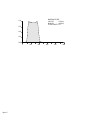
Our sample data set was muted to remove the air-coupled wave. Anytime a mute is applied to seismic data it should be as well defined and tight as
possible. This is to avoid removing subdued signal. The muting process zeros
samples, and once a sample is zeroed, the information contained within that
sample has gone to the "great bit bucket in the sky." Care should be taken when
defining and applying a mute. The plot of SSN 5 clearly shows the effect of the
mute as well as the narrowness of our defined mute window (Figure 5).
F) SORTING (GATHERING) INTO CDP FORMAT
The way data are organized for display and analysis is the heart of any seismic-reflection
program. Having flexibility to look at data in a variety of ways, whether according to receiver
location or common subsurface point, is critical for future digital enhancement as well as discrimination of subtle features. The actual sorting routine is not particularly difficult from a conceptual
point of view, but it does require a significant amount of information relating to the acquisition
geometries of your multichannel data. The sheer number of parameters and geometric configurations that need to be defined make sorting potentially the most mistake-prone part of processing
28
5
0
10
20
10
30
30
40
40
50
60
50
60
70
70
80
80
90
90
m100
100
20
s
e 110
c 120
110
120
130
140
130
140
150
150
160
160
170
170
180
180
190
190
200
200
210
210
220
220
230
230
240
240
0
figure 5
0
12 m
seismic data. Built into the sorting operation are several ways to cross-check the accuracy of the
information you have input However, they are not completely automated—you must request
and check the output of these operations to verify the correctness of your parameter and geometry
assignments.
Sorting your seismic data can be thought of as very similar to playing gin rummy. The main
goal is to order your data or cards into a sequence likely to be of the most use to you later. For
example, in rummy you may be collecting by suit; with seismic data you may be collecting by
receiver locations. In rummy you may be collecting by face value; in seismic you may be collecting by
common-mid-points. With the card game, the identification [value (numeric or other) and suit] are
displayed on the face of each card; with seismic data, the identification (location and size) is
contained within each trace header. In order for the data to be brought together in a meaningful
fashion, you must select which particular identification (parameter) is most significant for this
data set and future processing routines. The data can be gathered together, ordered, and reordered a
variety of times and ways.
The two most commonly used parameters to sort are CDP (common-depth-point) sometimes
referred to as CMP (common-mid-point), and common source-to-receiver offset (common offset, for
short). Sorting according to common source-to-receiver offset is exactly what it sounds like. All
traces are gathered according to like distances from source-to-receiver. For example, each of the 24
traces recorded within each field file to our sample data set is offset from the source by a unique
distance. Therefore, gathering according to a common offset distance will result in 24 different
primary groups (each with unique source-to-receiver offset) each containing 20 traces. In good data
areas once the appropriate corrections are made for offset and elevations, common-offset data (if
collected within the optimum window) can be viewed as a geologic cross-section without future
digital enhancement. However, seldom will common-offset data yield as much or as detailed
information as a properly processed CDP stacked section. Eavesdropper is specially designed to
enhance reflection information once your data are in a sorted CDP format.
Good, complete field notes are critical to correct and accurate defining of source and receiver
geometries, surface features, and events significant to future analysis. The information that must be
contained in the field notes for each recorded shot at each shotpoint includes:
1) shotpoint station number
2) live receiver station numbers relative to seismograph channel numbers
3) roll switch number
4) individual digital file name/number
The remainder of the items listed need to be included but only once, unless they change
during acquisition of the data.
5) sample interval/number of samples
6) analog-to-digital filter settings
7) anti-alias filter
8) type, number, and relative orientation of sources and receivers
9) profile location and purpose
10) any unusual offsets (inline or offline)
11) space for comments
12) time
13) weather conditions
14) system (seismograph) error messages
15) reminder to do system QC checks
30
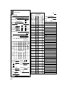
An example of a field notebook that we have used quite successfully for several years is
displayed in Figure 6.
All significant information about the source and receiver geometries as well as acquisition
parameters for our example data set are logged in the field notes (Figure 7). The 20 field files used
for this example data set (615-634)were extracted from a larger data set containing 39 files (601639). Building a batch processing file to define source and receiver geometries for our example data
set requires geometrically relating the 20 shotpoints and the 43 receiver locations used during the
acquisition of the section of the line used as our sample data set.
The primary task associated with sorting your data relates to the assignment of geometries
and parameters. Trace-header information plays a significant roll in this operation. The traceheader words most important to commit to memory are:
Header Word #
6
8
12
14
19
86
87
92
Identifies
the field file number/name under which this trace was stored in
after it was recorded
this trace's number within the field file it was collected under
(also is equivalent to the channel number this trace was recorded
at) this trace's corresponding CDP number (usually about twice the
associated station location)
the order of this trace within the appropriate CDP
distance this trace is from the source
station number of the receiver that recorded this trace
station number of the source associated with this trace
(the source sequence number of this trace, which sequentially relates
it to individual field files collected for a particular profile)
A helpful aid in defining the geometries and to double check the accuracy of your field
notes is a stacking chart (Figure 8). The layout of the stacking chart (by design) allows visual
correlation between the field notes and the sort batch file. It will simplify both visualizing and
defining geometries for particular Source Sequence Numbers (SSN).
STEP #6
*********************EXAMPLE DATA*********************
The upper portion of the chart built for our example data set (Figure 8),
defines station locations on the x axis and field file numbers as the y axis. Each
individual field record (file) number (y axis) has an associated set of 24 recording
channels and a shotpoint. The shotpoint location for a particular field record is
identified by an x located beneath the appropriate station location (x axis). Along
with this x (defining the shot location) is the assigned source sequence number
(SSN). Each live receiver location is represented along the x axis by the appropriate seismograph channel number. Notice the step-by-step progression of the
shot and receivers across the line.
The lower portion of the chart identifies the locations and SSN, original
field channel pairs as well as fold (redundancy, percent coverage) for each CDP.
31
KANSA
RVEY
SU
S
OLOGICA
L
GE
OBSERVATION FORM
19 8 9
tape
error
Location /Purpose
Contractor/Coordinator
Split-Spread
End-On
Energy Source
Gap
No. Stacked Per File
Source Spacing
P-Wave
Geophone Freq.
S-Wave
Single Source
Multi-Source
Take-Out Spacing
Array
Single Phones
Source/Receiver Geometry
AMPLIFIER GAINS
No.
2 4
5 7
6
9 11 13 15 17 19 21 23 File
8 10 12 14 16 18 20 22 24 No.
Att
Fre en.
q.
Amp. 1 3
F1
F2
Test
Oscil.
Operating
Gains
Amp. Scan Delay
Damper Box: In Out
Filters: High Cuts
Low Cuts
60 Hz Notch
Sample Int.
msec.
No. of Samples
Record Length
msec.
Rec. Start Delay
Amps.: IA5 IA6
Control Level
Temp.
Alias
Wind
Soil Conditions
figure 6
SEISMIC GEOMETRY
Flag No. of Trace
1
12 13 24
Dead
Traces
Tape
Shot
Point #
Tape
File No.
Roll
Switch No.
–
bite
par
18
89
(Time)
:
:
:
:
:
:
:
:
:
:
:
:
:
:
:
:
:
:
:
:
:
:
:
:
:
:
:
:
:
:
:
:
:
:
:
:
:
:
:
:
Remarks
OBSERVATION FORM
tape
error
19 8 9
UK BUFF.589
Location /Purpose Thames River Valley, G. B.
Chris Leach EG & G
Contractor/Coordinator
Tape
Energy Source
Gap
12-Gauge Buffalo Gun
7
2.5 m
100
Hz
Geophone Freq.
2.5
m
Take-Out Spacing
Source Spacing
Split-Spread
✔ End-On
No. Stacked Per File 1
✔ P-Wave ✔ Single Source
S-Wave
Multi-Source
✔ Single Phones
Array
Source/Receiver Geometry
●
●
●
●
●
source ✳
2.5 m
●
●
●
●
●
●
●
●
receivers
station location
AMPLIFIER GAINS
No.
2 4
5 7
6
9 11 13 15 17 19 21 23 File
8 10 12 14 16 18 20 22 24 No.
Att
Fre en.
q.
Amp. 1 3
F1
F2
Test
Oscil.
Floating Pt Amps
Operating
Gains
0
Filters: High Cuts 500 Hz
Amp. Scan Delay
60 Hz Notch
Damper Box:
In ✔ Out
200 Hz
Sample Int. 1/2
msec.
512
msec.
Low Cults
Alias
1024
Rec. Start Delay 0
N/A
Control Level
Wind 0-5 KmPH
Soil Conditions dry sod
No. of Samples
figure 7
Record Length
Amps.: IA5 IA6
o
Temp. 23 C
Page
SEISMIC GEOMETRY
Flag No. of Trace
1
12 13 24
Line Name
Dead
Traces
–
Shot
Point No.
Tape
File No.
Roll
Switch No.
18
89
bite
par
KANSA
RVEY
SU
S
OLOGICA
L
GE
Observer
(Time)
EG & G England 1
Don S.
Date 5/10/89
Remarks
:
108 001
75 115
12
109 002
76 116
11
110 003
77 117
10
111 004
78 118
9, 24
112 005
79 119
8, 23
113 006
80 120
7, 22
114 007
81 121
6, 21
115 008
82 122
5, 20
116 009
83 123
4, 19
117 010
84 124
3, 18
118 011
85 125
2, 17
119 012
86 126
1, 16
120 013
87 127
15
121 014
88 128
14
122 015
89 129
13
123 016
90 130
12
124 017
91 131
11
125 018
92 132
10
126 019
93 133
9
126 020
93 133
9
:
:
:
:
3:02
:
:
: airplane noise
airplane noise
:
:
1
automobile noise
:
:
:
3:12
:
:
:
second shot in hole
108
field file #
615
616
617
618
619
620
621
622
623
624
625
626
627
628
629
630
631
632
633
634
SSN
1
2
3
4
5
6
7
8
9
10
11
12
13
14
15
16
17
18
19
20
109
110
111
112
113
114
1X
115
116
117
118
119
120
121
122
123
124
125
126
127
128
129
130
131
1
2
1
3
2
1
4
3
2
1
5
4
3
2
1
6
5
4
3
2
1
7
6
5
4
3
2
1
8
7
6
5
4
3
2
1
9
8
7
6
5
4
3
2
1
10
9
8
7
6
5
4
3
2
1
11
10
9
8
7
6
5
4
3
2
1
12
11
10
9
8
7
6
5
4
3
2
1
13
12
11
10
9
8
7
6
5
4
3
2
1
14
13
12
11
10
9
8
7
6
5
4
3
2
1
15
14
13
12
11
10
9
8
7
6
5
4
3
2
1
16
15
14
13
12
11
10
9
8
7
6
5
4
3
2
1
17
16
15
14
13
12
11
10
9
8
7
6
5
4
3
2
1
2X
3X
4X
5X
6X
7X
8X
9X
10X
X=source location
11X
12X
13X
14X
15X
16X
17X
18X
19X
20X
CDP#
source station location=SSN
108=1
109=2
110=3
111=4
112=5
113=6
114=7
115=8
116=9
117=10
118=11
119=12
120=13
121=14
122=15
123=16
124=17
125=18
126=19
127=20
224
225
226
227
228
229
230
231
232
233
234
235
236
237
238
239
240
241
242
243
244
245
246
1,1
1,2
1,3
2, 1
1,4
...
1,5
...
3, 1
1,6
...
...
1,7
...
...
4, 1
1,8
...
...
...
1,9
...
...
...
5, 1
1,10
...
...
...
...
1,11
...
...
...
...
6,1
1,12
...
...
...
...
...
1,13
...
...
...
...
...
7,1
1,14
...
...
...
...
...
...
1,15
...
...
...
...
...
...
8,1
1,16
...
...
...
...
...
...
...
1,17
...
...
...
...
...
...
...
9,1
1,18
...
...
...
...
...
...
...
...
1,19
...
...
...
...
...
...
...
...
10,1
1,20
...
...
...
...
...
...
...
...
...
1,21
...
...
...
...
...
...
...
...
...
11,1
1,22
...
...
...
...
...
...
...
...
...
...
1,23
...
...
...
...
...
...
...
...
...
...
12,1
1,24
...
...
...
...
...
...
...
...
...
...
...
9
9
10
10
11
12
12
12
SSN, trace#
1, 6
fold
figure
223
8
1
1
2
2
3
3
4
4
5
5
6
6
7
7
8
8
247
248
...
...
...
...
...
...
...
...
...
...
...
13,1
2,24
...
...
...
...
...
...
...
...
...
...
...
12
12
249
250
...
...
...
...
...
...
...
...
...
...
...
14,1
3,24
...
...
...
...
...
...
...
...
...
...
...
12
12
251
...
...
...
...
...
...
...
...
...
...
...
15,1
12
252
4,24
...
...
...
...
...
...
...
...
...
...
...
12
253
254
...
...
...
...
...
...
...
...
...
...
...
16,1
5,24
...
...
...
...
...
...
...
...
...
...
...
12
12
255
256
...
...
...
...
...
...
...
...
...
...
...
17,1
6,24
...
...
...
...
...
...
...
...
...
...
...
12
12
257
258
...
...
...
...
...
...
...
...
...
...
...
18,1
7,24
...
...
...
...
...
...
...
...
...
...
...
12
12
259
260
261
...
...
...
...
...
...
...
...
...
...
...
19,1
20,1
8,24
...
...
...
...
...
...
...
...
...
...
...
20,2
...
...
...
...
...
...
...
...
...
...
...
20,3
13
13
12
262
9,24
...
...
...
...
...
...
...
...
...
...
20,4
12
station location
132
133
134
135
136
137
138
139
140
141
142
143
144
145
146
18
17
16
15
14
13
12
11
10
9
8
7
6
5
4
3
2
1
19
18
17
16
15
14
13
12
11
10
9
8
7
6
5
4
3
2
1
1
20
19
18
17
16
15
14
13
12
11
10
9
8
7
6
5
4
3
2
2
21
20
19
18
17
16
15
14
13
12
11
10
9
8
7
6
5
4
3
3
22
21
20
19
18
17
16
15
14
13
12
11
10
9
8
7
6
5
4
4
23
22
21
20
19
18
17
16
15
14
13
12
11
10
9
8
7
6
5
5
24
23
22
21
20
19
18
17
16
15
14
13
12
11
10
9
8
7
6
6
24
23
22
21
20
19
18
17
16
15
14
13
12
11
10
9
8
7
7
24
23
22
21
20
19
18
17
16
15
14
13
12
11
10
9
8
8
24
23
22
21
20
19
18
17
16
15
14
13
12
11
10
9
9
24
23
22
21
20
19
18
17
16
15
14
13
12
11
10
10
24
23
22
21
20
19
18
17
16
15
14
13
12
11
11
24
23
22
21
20
19
18
17
16
15
14
13
12
12
24
23
22
21
20
19
18
17
16
15
14
13
13
24
23
22
21
20
19
18
17
16
15
14
14
263
264
265
266
267
268
269
270
271
272
273
274
275
276
277
278
279
280
281
282
...
...
...
...
...
...
...
...
...
...
20,5
10,24
...
...
...
...
...
...
...
...
...
20,6
...
...
...
...
...
...
...
...
...
20,7
11,24
...
...
...
...
...
...
...
...
20,8
...
...
...
...
...
...
...
...
20,9
12,24
...
...
...
...
...
...
...
20,10
...
...
...
...
...
...
...
20,11
13,24
...
...
...
...
...
...
20,12
...
...
...
...
...
...
20,13
14,24
...
...
...
...
...
20,14
...
...
...
...
...
20,15
15,24
...
...
...
...
20,16
...
...
...
...
20,17
16,24
...
...
...
20,18
...
...
...
20,19
17,24
...
...
20,20
...
...
20,21
18,24
...
20,22
...
20,23
19,24
20,24
11
11
10
10
9
9
8
8
7
7
6
6
5
5
4
4
3
3
2
2
147
148
149
150
151
152
153
154
155
156
24
23
22
21
20
19
18
17
16
16
24
23
22
21
20
19
18
17
17
24
23
22
21
20
19
18
18
24
23
22
21
20
19
19
24
23
22
21
20
20
24
23
22
21
21
24
23
22
22
24
23
23
24
24
1-24 trace# (channel#)
24
23
22
21
20
19
18
17
16
15
15
The lower portion of the stacking chart was derived from the upper part. The
CDP numbers identified along the x axis on the lower part are exactly double the
surface location defined directly above on the upper portion of the chart. The
number pairs beneath each CDP location identify the SSN and seismograph
channel number for the trace(s) sampling this particular midway point between
source and receiver (CDP). As an example, locate SSN 5 and seismograph channel number 10 on the upper portion of the stacking chart. Next, find the point
which is midway between the shot for SSN 5 and the associated seismograph
channel 10. Finally, extrapolate that point straight down into the lower portion
of the chart and you will find the number pair 5, 10 as the fifth set of number
pairs beneath CDP location 240. The bottom set of numbers running parallel to
the x axis identify the fold of the associated CDP. The fold can be figured by
simply adding the number of SSN/trace number pairs beneath each CDP
location.
The program dseis has an option to print a table which will allow you to
directly compare your hand-generated stacking chart directly from the field notes
with a computer-generated chart reflecting the geometries and parameters you
defined for the *sort operation. Our computer-generated chart for the sample
data set will be compared to the hand-generated chart (Figure 8) after our sort
deck is complete.
A stacking chart may not always be necessary, but until a great deal of experience is gained
processing seismic data, it is a wise aid in assuring the data you are preparing to gather and stack is
properly identified and ordered.
Once you have a complete set of field notes and know how you would like to order your data
for future digital enhancement and display, you are ready to create a batch process file to sort your
data. As with other operations, start building your batch file by typing the following at the
system prompt:
STEP #6a
*********************EXAMPLE DATA*********************
The following deck is built for CDP sorting of an example data set which is
composed of 20 shots recorded on a 24-channel seismograph across 44 receiver
stations, each separated by 2.5 m. The source-to-closest-receiver distance is
17.25 m and the source stations are coincident with the receiver stations. The
data were collected using a CDP-type roll-along technique. The relative sourceto-receiver orientation was end-on.
Line
Description
1
>>START
see *EDKL for description of >>START
2
*INPF EDMT.dat
see *EDKL for description of *INPF
36
3
*SORT 12 19
The *SORT procedure calls the subroutine responsible for collecting traces
according to indicated header words. We have described a sorting operation here which will gather together all traces with equivalent midpoints
between shot and receiver. The first value (header-word number) input
designates the primary sort grouping (trace header word 12, CMP or CDP
number). The second value (header-word number) requested designates
the secondary grouping (trace header word 19, distance from source to
receiver). The secondary grouping simply designates the ordering of the
trace display within the primary grouping. With unprocessed field data,
the primary grouping is file or source-sequence number, and the secondary grouping is according to individual trace or channel numbers.
4
PTRN 2.5 24 1
PTRN operation defines the distance between surface stations and physical
seismograph parameters. This operation must always precede the *SORT
procedure definition. The first requested input is the distance between
station locations (2.5 m). The second value to be identified is the total
number of recording channels on your seismograph (24). And the final
value represents the units of length used during the acquisition of the data
(1 = meters, 0 = feet). This operation (ptrn) is the lead-in for the next
line(s) (pn) which will identify all the different source and receiver
geometries used throughout the collection of this data set.
5a PN 1 108 115 24 1
S
#
108
1
24
************************
115
138
trace/channel
surface station
Note: A piece of the stacking chart is represented above to help
equate the station numbers to the actual source and receiver patterns.
A stacking chart allows you to visualize the relative location of the
shots and receivers.
pn defines each unique relative source-to-receiver geometry. The pattern
described on line 5a is designated as pattern number 1 (it will be referenced
by that number (1) later in this batch job). It defines a source location (108)
and its associated first receiver location (115) as well as indicates consecutive receiver locations (24). The fifth value designates the amount each
surface station was incremented after each shot. In this case, stations were
incremented by 1. In other words, station 115 equates to trace/channel 1 of
your seismograph; station 116 equates to trace/channel 2 of your
seismograph.
If your source was occupying (being fired) every station location but your
receivers were located (live) at every other surface station, you would
37
have used a 2 for the fifth input value to indicate the receiver spacing was
twice the surface-station spacings. Then surface station 115 would equate
to trace/channel 1 and station 117 would have equated to trace/channel 2,
etc. Another possibility is that your roll switch is wired reverse to this
sequence which means your trace/channel 1 is at surface station location
138 when surface stations 115 to 138 are selected. If this is the case, you
would want to designate a negative one (-1) incrementation of surfacestation locations as the fifth value input of the pn definition. The correct
pn definition for a reversed roll-switch would look like line 5b.
† 5b PN 1 108 138 24 -1
S
#
108
24
1
************************
115
138
trace/channel
surface station
This definition indicates the surface station location of the shot was 108,
trace/channel 1 was 138, and incrementing of station locations is negative
(-1) with respect to the positive increasing trace/channel numbers. Therefore, channel/trace 1 is surface station 138, channel/trace 2 is surface station
137, channel/trace 3 is surface station 136, etc.. Here the same source-toreceiver maximum and minimum offsets are defined (source 108, minimum offset 115, maximum offset 138) as on line 5a, the exception of course
being the decrementing surface station numbers with respect to the incrementing trace/channel numbers. This is a critical difference when the
source-to-individual-receiver distances are calculated later in this batch job.
All the information necessary to determine exactly how to define the
trace/channel orders is contained within the trace header and is easily
viewed using the trace-header-dump (trhd) routine previously discussed.
† 5c
PN 1 95 99 2
S
#
95
1
24
************************
99
122
trace/channel
surface station
The sorting routine doesn't care what the actual numbers input for the
source (108) and receiver (115) locations are; it only looks at relative differences. What that means is the pn definition on line 5a is identical to the
pn definition on line 5c. It is not necessary to define existing station numbers. Most of the time it is advisable to identify real station numbers just
to avoid confusion if problems crop up later.
This definition of pattern is exactly the same as the one defined on line 5.
The station numbers of the shot and receivers need only be relative to
each other and do not need to be related to the actual values used in the
field. Any arbitrary numerical representation will work.
1
12
S
13
24 trace/channel
† 5d PN 1 114 101 12 1 116 12 1 * * * * * * * * * * * * # * * * * * * * * * * * *
101
112
38
116
127 surface station
This definition is of a split-spread pattern. This definition does not apply
to the acquisition parameters and geometries being defined here, but is included as an example in case you encounter a split-spread source-receiver
geometry. Briefly, this is the first pattern defined (1), the shot station
number is 114, the first trace/channel station number is 101, there are 12
consecutive trace/channels defined across 12 sequential surface station
locations, then a 3-station skip to station location 116 which is trace/
channel 13 where the remaining 12 channels are defined starting at 116 to
127, inclusive, each sequential increase of (1) in trace/channel number
corresponds to a sequential increase of 1 in the surface-station location.
† Not appropriate for this data set—used only as an example.
6
SHOT
This alpha character description (shot) simply identifies the succeeding
series of sn or snsn definitions as related to the shot location and source
sequence numbers (SSN). This operation must follow the ptrn operation.
7
SN 1 108 1 0 0 1
The SN definition input is required for each field file (source sequenced
file). This operation matches a source-sequenced file with its appropriate
shotpoint's surface station location and source/receiver geometry, as
described by the ptrn operation. In this case, the (Source Sequence
Number) SSN is 1, the shot station location is 108, the source/receiver
geometry is defined in pn 1. The fourth entry is related to inline offset (0),
this is simply the distance from the defined surface station location to the
actual location of the shot recorded along the line of the survey (parallel
offset). The fifth entry (0) is also related to the actual location of the shot
recorded at this surface location (109), and it defines the distance off the
line between the shot and actual surface station location (perpendicular
offset). The sixth value (1) identifies the repeat shot number. Since we are
only recording one shot per surface location 1 is the appropriate sixth
value. The repeat shot number simply identifies which shot this file
represents at this location. If multiple shots are recorded individually at
this location on different files, the program is capable of identifying which
shot this file represents and then allows the option to later sort according
to particular repetitive shot number at each location.
8
SN 2 109 1
This SN definition as with the previous one (line 7) is required to describe
the source station number and it's associated live receiver pattern. This
must be done for each defined SSN. The only difference between this sn
39
definition and the one previous is SSN 2 is defined which has shot
location 109, whereas the previous one was for SSN 1 which had shot
location 108. The last three parameters were omitted on this definition
because the default values were appropriate.
The line format was purposely changed on line 8 simply to demonstrate
the flexibility of formatting within the program. This shows the program
is not field sensitive with respect to the number of spaces between input
parameters. However, it should be kept in mind that the order of the input values is critical. If you wish to input values not identified as default
values for the sixth and seventh requested parameters but your fourth and
fifth are the same as the default values, you must input all values from
the first requested to the seventh, regardless of the default values. (See line 10).
9
SNSN < 3 19 1 > < 110 126 1 > 1
The SNSN definition permits the assignment of field geometries to large
numbers of sequential field files possessing identical shot and receiver
patterns as well as source offsets and bad traces. The < > are treated as
entry parameters and therefore need to be separated from other entries by
a space. Here we are defining the shot patterns for SSN 3 through 19
which related to shot locations 110 to 126. Both shot location and SSN's
increment by 1 as the source and receivers move down the survey line.
Therefore, the first set of bracketed values represent the SSN's and their
incrementing while the second set of bracketed values represent the associated shot locations and their incrementation pattern. The information
within the first set of brackets is equivalent to the first entry on a normal
SN definer. The second set of bracketed values which are equivalent to the
second entry on the normal SN definer. All parameters beyond the first
two of the SNSN definers are identical to those of the ordinary SN definer.
10
SN 20 127 1 0 0 1 1 24
This shotpoint definition has a couple extra entries in comparison to the
previous sn definers. The SN definition's seventh value is the first dead
trace/channel number and eighth value (24) is the last dead trace/channel
number. From the field notes for our sample data, the 19th and 20th shots
were recorded at the same location. In order to retain equal weighting of
all shot locations across the line, one of the duplicate shots must be
removed. In this case, the second shot was deleted using the 7th and 8th
values in the SN definition. The program will interpolate between the
seventh and eighth input values. This means, if the seventh value is 19
and the eighth value is 22, the program will omit 19 thru 22, inclusive.
The previous SN definers have had the same inline and offline offsets as
well as repeat shot number. The information was not entered because the
default values are appropriate (in other words if you do not enter anything
40
for the required values the program assumes the default values are
correct).
11 TABL 1 1
The tabl operation is optional and allows you to cross-check your defined
geometries with the actual field geometries. The two input values are
flags. The first (1) designates that you wish to have the receiver diagram
plotted out, and the second (1) signals the printing of the sort table. The
entire table will be contained within the journalization file (i.e., DSEIS
SORT.dek TABLE.lst where TABLE.lst is your journal file and it can be
typed out or printed using standard MSDOS operations)
12 *OUTF SORT.dat see *EDKL for description of *OUTF
13 >>END
see *EDKL for description of >>END
At this point you need to exit your text editor. In order to see the batch
processing file you have created to sort seismic data into a CDP format, type the
following commands at the system prompt:
>TYPE SORT.dek
<return>
>>start
*inpf edmt.dat
*sort 12 19
ptrn 2.5 24 1
pn 1 108 115 24 1
shot
sn 1 108 1 0 0 1
sn 2 109 1
snsn < 3 19 1 > < 110 126 1 > 1
sn 20 127 1 0 0 1 1 24
tabl 1 1
*outf sort.dat
>>end
Now, in order to run the sorting batch job you just typed out, enter the
following series of commands at the system prompt:
>DSEIS SORT.dek TABLE.lst
<return>
As with the other batch operations already run, the program will continuously update the screen with pertinent information regarding the present status
of the batch job. The TABLE.lst file is again a journal file that will contain not
only the blow-by-blow account of the processing sequence, it will also contain the
41
geometries and sorting sequences applied in accordance with the input information. This is intended to allow you the option to compare your stacking chart
developed from the field notes with the actual information you coded into the
various operations in the batch processing file. The journal file will be contained
in the subdirectory in which you are running the seis program in and can be
viewed either in hard copy or on the CRT.
The stacking chart, generated by the program (assuming you used the tabl
option) with the information input during the sort operation, is displayed below:
SORTED RECORD TABLE (SHOT #1)
RCRD FOLD SN-TR SN-TR SN-TR SN-TR SN-TR SN-TR SN-TR SN-TR SN-TR
223
1
1-1
224
1
1-2
225
2
2-1
1-3
226
2
2-2
1-4
227
3
3-1
2-3
1-5
228
3
3-2
2-4
1-6
229
4
4-1
3-3
2-5
1-7
230
4
4-2
3-4
2-6
1-8
231
5
5-1
4-3
3-5
2-7
1-9
232
5
5-2
4-4
3-6
2-8
1-10
233
6
6-1
5-3
4-5
3-7
2-9
1-11
234
6
6-2
5-4
4-6
3-8
2-10
1-12
235
7
7-1
6-3
5-5
4-7
3-9
2-11 1-13
236
7
7-2
6-4
5-6
4-8
3-10
2-12 1-14
237
8
8-1
7-3
6-5
5-7
4-9
3-11 2-13
1-15
238
8
8-2
7-4
6-6
5-8
4-10
3-12 2-14
1-16
239
9
9-1
8-3
7-5
6-7
5-9
4-11 3-13
2-15
240
9
9-2
8-4
7-6
6-8
5-10
4-12 3-14
2-16
241
10
10-1
9-3
8-5
7-7
6-9
5-11 4-13
3-15
242
10
10-2
9-4
8-6
7-8
6-10
5-12 4-14
3-16
243
11
11-1 10-3
9-5
8-7
7-9
6-11 5-13
4-15
244
11
11-2 10-4
9-6
8-8
7-10
6-12 5-14
4-16
245
12
12-1 11-3
10-5
9-7
8-9
7-11 6-13
5-15
246
12
12-2 11-4
10-6
9-8
8-10
7-12 6-14
5-16
247
12
13-1 12-3
11-5
10-7
9-9
8-11 7-13
6-15
248
12
13-2 12-4
11-6
10-8
9-10
8-12 7-14
6-16
249
12
14-1 13-3
12-5
11-7
10-9
9-11 8-13
7-15
250
12
14-2 13-4
12-6
11-8
10-10 9-12 8-14
7-16
251
12
15-1 14-3
13-5
12-7
11-9 10-11 9-13
8-15
252
12
15-2 14-4
13-6
12-8
11-10 10-12 9-14
8-16
253
12
16-1 15-3
14-5
13-7
12-9 11-11 10-13
9-15
254
12
16-2 15-4
14-6
13-8
12-10 11-12 10-14
9-16
255
12
17-1 16-3
15-5
14-7
13-9 12-11 11-13 10-15
256
12
17-2 16-4
15-6
14-8
13-10 12-12 11-14 10-16
257
12
18-1 17-3
16-5
15-7
14-9 13-11 12-13 11-15
258
12
18-2 17-4
16-6
15-8
14-10 13-12 12-14 11-16
259
12
19-1 18-3
17-5
16-7
15-9 14-11 13-13 12-15
260
12
19-2 18-4
17-6
16-8
15-10 14-12 13-14 12-16
261
11
19-3 18-5
17-7
16-9
15-11 14-13 13-15 12-17
262
11
19-4 18-6
17-8
16-10 15-12 14-14 13-16 12-18
263
10
19-5 18-7
17-9
16-11 15-13 14-15 13-17 12-19
264
10
19-6 18-8
17-10 16-12 15-14 14-16 13-18 12-20
265
9
19-7 18-9
17-11 16-13 15-15 14-17 13-19 12-21
266
9
19-8 18-10 17-12 16-14 15-16 14-18 13-20 12-22
267
8
19-9 18-11 17-13 16-15 15-17 14-19 13-21 12-23
268
8
19-10 18-12 17-14 16-16 15-18 14-20 13-22 12-24
269
7
19-11 18-13 17-15 16-17 15-19 14-21 13-23
42
SN-TR SN-TR SN-TR
1-17
1-18
2-17
1-19
2-18
1-20
3-17
2-19
3-18
2-20
4-17
3-19
4-18
3-20
5-17
4-19
5-18
4-20
6-17
5-19
6-18
5-20
7-17
6-19
7-18
6-20
8-17
7-19
8-18
7-20
9-17
8-19
9-18
8-20
10-17
9-19
10-18
9-20
11-17 10-19
11-18 10-20
11-19 10-21
11-20 10-22
11-21 10-23
11-22 10-24
11-23
11-24
1-21
1-22
2-21
2-22
3-21
3-22
4-21
4-22
5-21
5-22
6-21
6-22
7-21
7-22
8-21
8-22
9-21
9-22
9-23
9-24
1-23
1-24
2-23
2-24
3-23
3-24
4-23
4-24
5-23
5-24
6-23
6-24
7-23
7-24
8-23
8-24
270
271
272
273
274
275
276
277
278
279
280
281
282
>>end
7
6
6
5
5
4
4
3
3
2
1
1
1
19-12
19-13
19-14
19-15
19-16
19-17
19-18
19-19
19-20
19-21
19-22
19-23
19-24
18-14
18-15
18-16
18-17
18-18
18-19
18-20
18-21
18-22
18-23
18-24
17-16
17-17
17-18
17-19
17-20
17-21
17-22
17-23
17-24
16-18
16-19
16-20
16-21
16-22
16-23
16-24
15-20 14-22
15-21 14-23
15-22 14-24
15-23
15-24
13-24
The output from the tabl option will generate a table similar to the above
table which contains the SSN-trace pairs with their associated RCRD (CDP #) and
appropriate fold. Checking this table (program generated) against the one you
constructed (Figure 8) will help verify the correctness of the sort file as well as
assure you the data geometries are input into the trace header correctly.
It should be kept in mind that the stacking chart generated by the sorting operation (tabl)
does not check the real input data to identify traces designated as bad. Therefore, the SSN trace
pairs, output with its associated CDP number, will include values previously deleted. If your
hand-generated stacking chart is correct, it will also include the dead or bad traces.
It will be beneficial at this point to generate a hard copy plot of the entire sorted data set.
This will allow you to cross check your stacking chart with your sorting table printout as well as
the actual sorted data. Many times problems, not obvious on a sorting table, will be quite obvious on
a hard-copy plot of CDP sorted data.
STEP #6b
*********************EXAMPLE DATA*********************
The principal (higher amplitude) reflections identified on our raw field
file (Figure 1) are still interpretable on the gathers of CDPs 245 and 246 (Figure 9).
These two gathers represent the subsurface points located beneath station locations 122 1/2 and 123. Careful examination reveals the zeroed-out portions of
the traces previously occupied by the air-coupled wave. The traces are ordered
within each CDP according to original source-to-receiver offset distance (trace
header word 19 as defined by the *sort). The location of the traces within each
CDP are also identified by a trace header word (14). Header word 14 designates
the order within the CDP gather. The numbering of traces within the CDP is
from left to right with the far left trace of CDP 245 possessing a 1 at trace header
location 14 while the trace on the far right possesses an 11 at trace header location
14. Header word 14 is totally unrelated to header word 8 (original seismograph
channel number) and may or may not be the same value.
43
CDP number
0
245
246
10
20
10
20
30
30
40
40
50
60
50
60
70
70
80
80
90
90
m100
100
s
e 110
c 120
120
130
130
140
140
150
150
160
160
170
170
180
180
190
190
200
200
210
210
220
220
230
230
240
240
110
0
figure 9
0
12 m
G) ELEVATION CORRECTION/DATUM ASSIGNMENT
Correcting your data for a variable near-surface can be one of the most difficult problems
encountered while processing seismic-reflection data. Most areas on a seismic-reflection section
possessing poor signal-to-noise ratios or that have resulted in an incorrect structural interpretation
are pigeon-holed as related to "static problems." These problems can be the result of anything from
incorrect compensation for surface topography to uncompensated velocity irregularities in the near
surface.
On any data set, the first step in eliminating static effects requires adjustment of the data
to a datum. A datum is simply a reference line with some absolute correlation to sea level or, in
some cases average slope of the ground surface (sloping datum). Generally on conventional data,
the datum is chosen beneath the weathered and within the subweathered zone. Defining the
datum within the subweathered zone is necessary to insure all non-uniform near-surface material is
above the datum. The correction conceptually involves removal of all material above the datum,
which in turn ultimately allows accurate time-to-depth conversions relative to sea level on interpreted CDP stacked sections. Correcting for both surface topography and a non-uniform weathered
layer requires at least relative station elevations and a somewhat detailed knowledge of the nearsurface velocity and depth structure. The datum correction is generally perceived as a first guess
approximation and is intended to remove major static anomalies associated mainly with relative
elevation changes. Discrepancies between the calculated datum correction and true datum correction are generally addressed using iterative numerical techniques at a later stage in the CDP
processing flow.
Shallow high-resolution reflection profiles generally target geologic features within what
conventional wisdom would suggest is the weathered zone. Correcting for elevation and near-surface
irregularities on shallow profiles therefore becomes quite complicated in comparison to the previously described conventional procedure for datum corrections. Detailed knowledge of shallow
velocity and depth information is critical for accurate datum corrections on shallow-reflection
surveys. Subtle changes in the velocity of very near-surface material can drastically affect the
spectral as well as spatial properties of higher frequency data. For example, if you are looking for
structure on the bedrock surface at a depth of 12 m with an NMO velocity of 400 m/s and dominant
reflection frequencies around 200 Hz, an uncompensated 0.3-m variation in elevation or a 10 m/s
velocity anomaly can result in a 100 degree phase shift in the recorded reflection wavelet. A gradual horizontally increasing near-surface velocity can be misinterpreted as a slope on the bedrock
surface.
The selection of a datum for shallow-reflection surveys can greatly influence the outcome
and validity of the final interpretation of your data. Many times reflection information of interest
will be removed if a flat datum is chosen within the subweathered layer followed by conventional
calculated removal of all overlying material. For most shallow-reflection profiles, a datum should
be chosen equal to the highest topographic feature on the survey line. Then the time adjustment to
compensate for the missing material should be added to each trace in accordance to the
velocity/depth function. In areas with alluvium over bedrock, generally a direct-wave velocity
can be used to determine the appropriate time correction. In areas with either a thin layer of
weathered material or no weathered material at all overlying outcropping or subcropping units, a
more detailed velocity function is necessary to reconstruct the material between the present ground
surface and the datum. For shallow-reflection data, the datum represents a pseudo ground surface
composed of actual material beneath topographic highs and the virtual material used to
compensate for the distance between the ground surface and topographic lows and the datum. The
sum is the time between the ground surface and the allowing depth calculations to bedrock or other
layers.
45
The most inaccurate part of the datum correction for shallow surveys involves the assignment of depth/velocity pairs to each surface station. The best way to determine these values is
through uphole/downhole surveys in strategically placed boreholes. The Eavesdropper software
will generate a near-surface model along the survey line by incorporating all the uphole-determined velocity and depth information with the spatial distribution of the holes. Without uphole
data, the only information available to approximate the near-surface velocity/depth structure is
direct- and refracted-wave information. In some cases, the values obtained using this information
are sufficient to generate an acceptable near-surface model. The closer to a true near-surface
velocity/depth model you can define for the datum correction, the less dependant you will be on
iterative numerical statics routines and the more confidence you will be able to put in your depth
calculation during the interpretation portion of your survey.
Determining the appropriate values to input into, and the usefulness of the output of the
*SURF operation requires a thorough understanding of the geologic situation as well as certain
physical properties of the near-surface materials. The input velocity function will be interpolated
across the entire expanse of the defined profile line. Elevation data input for each station location
need only be relative within the survey (absolute elevation data are not necessary). If the datum
was assigned above the highest topographic feature on the survey line, the outputted static correction for each receiver and shot station will be necessary during the later interpretation stages to
calculate depths. If the datum was assigned within the subweathering zone, time-to-depth conversions can be made without knowledge of the amount of the static correction (material removed).
This is because the relative elevation of the datum is known, which in turn allows accurate determination of time values between the datum and event of interest.
The necessary datum/elevation correction for our sample data set only modifies a small
portion of the line. The data were collected in a river valley. River valleys often (as with this
case) do not have significant changes in elevation. The majority of the sample data set was
collected across a flat-lying pasture with little or no surface evidence to suggest areas of potential
static anomalies. At the extreme east end of the line, however, the line crossed a wash-out extending approximately 6 m with a maximum relative depth of 1 m. If not for the washout spot on the
line, no datum correction at this time would be necessary or possible. However, with the elevation
change present as a result of the wash-out, the *SURF operation is necessary on this line.
STEP #7
*********************EXAMPLE DATA*********************
Determination of the velocity within the very-near surface using the
information provided with and contained within the sample data set is not
straight forward. Therefore, we will provide you with the velocity information
as well as the relative elevation data necessary to properly calculate and apply the
datum correction. An uphole velocity survey in conjunction with your seismicreflection survey is advisable whenever possible to accurately determine the
near-surface velocity model.
AVERAGE VELOCITY FROM THE SURFACE TO APPROXIMATELY 3-METERS
OF DEPTH IS:
770 M/S
CRITICAL ELEVATION INFORMATION INCLUDES THE FOLLOWING:
46
STATION LOCATION
RELATIVE ELEVATION (M)
136
137
138
139
140
141
142
143
0
0.3
0.6
0
-1
-0.3
-0.6
0
Once as much information as possible is obtained about the near-surface
materials, a batch processing file must be created to calculate the appropriate
static values for each shot and receiver station. This operation (*SURF) does not
apply the calculated shifts. This routine calculates the appropriate shift and
updates the trace headers. In order to apply this static shift, a *STAT 1 operation
must follow the *SURF operation. This can be accomplished either in the same
or a separate batch job file. The following sequence of entries represent a batch
processing file to calculate and apply datum corrections to our sample data set.
Line
Description
1
>>START
see *EDKL for description of >>START
2
*INPF SORT.dat
see *EDKL for description of *INPF
3
*SURF 100
*SURF identifier calls up the terrain correction subroutine from within
DSEIS. The required input value relates to defining the datum. The value
of the datum is arbitrarily assigned as 100. In this case, think of the data as
representing absolute elevation relative to sea level.
4
ALVF 105 770 90
alvf defines the average velocities and their associated depths. For the
sample data set, we are defining a single velocity across the entire line and
therefore the first entry identifies the maximum surface elevation (105) of
the defined velocity function. The second entry (770) defines the average
velocity from the maximum surface (105) to a maximum depth identified
by the third entry (90).
We have determined the following near-surface configuration:
47
sea level (m)
105
100
95
datum
V = 770 m/s
o
90
For a case with multiple depth velocity pairs—
† 4a
ALVF 1000 1300 950 1600 900
sea level (m)
alvf operation defines the velocity model for the near-surface material
down to a depth necessary to correct all station locations to the defined
datum. The values requested for the ALVF operation are: the surface elevation (1000) of the defined velocity function, the average velocity (1300)
from the surface (1000) to the elevation defined by the third numeric
value (950), then the average velocity (1600) from the surface (1000) to the
elevation defined by the fifth numeric value (900). This sequence of average velocity/depth pairs continues until your entire velocity function is
defined. An important note at this point: the velocities defined here
(ALVF) are AVERAGE VELOCITIES FROM THE SURFACE TO THE
DEFINED DEPTH. The program will calculate interval velocities for the
defined intervals (1000-950, 950-900). This program works most effectively
with uphole/downhole check shot velocity information.
1000
950
V
= 1300
ave
V
= 1600
ave
900
† Examples not applicable to our sample data set.
5
SE 126 97 100
se operation defines each station location and its associated source and
receiver elevations. The defined values are station location (108), source
elevation (97), and receiver elevation (100). The receiver elevation need
not be defined if it is the same as the source elevation. A shot elevation
defined at a station where no shot was recorded will be sorted out by the
program and properly handled. The program interpolates horizontally
and vertically between defined values and, therefore, stations 108 through
125 are not defined since they are all the same as 126.
6
SE 127 100
7
SE 136 100
48
8
SE 137 100.3
9
SE 138 100.6
10
SE 139 100
11
SE 140 99
12
SE 141 99.6
13
SE 142 100.6
14
SE 143 100
15
*STAT 1
*STAT operation applies static correction values defined in the trace
headers. These static header words are updated by other operations (*auts,
*surf, or user input values). The *STAT operation can be executed within
the batch job where the actual static correction values are determined or
later in a separate batch job either independently or with any other operation(s). The only required input value (1) designates the type of operation
used to define static shift values.
16
*OUTF SURF.dat — see *EDKL for description of *OUTF
17
>>END — see *EDKL for description of >>END
At this point you have completed the building of an executable file for the
generation and application of static shifts to sorted data for the correction of
elevation and near-surface irregularities across the profile. In order to quickly
check to make sure all the values and operations you just identified during the
surf operation, type the following at the system prompt:
>>TYPE SURF.DEK
<return>
You should see the following if the above deck is what you entered:
>>start
*inpf sort.dat
*surf 100
alvf 105 770 90
se 126 97 100
se 127 100
se 136 100
se 137 100.3
49
se 138 100.6
se 139 100
se 140 99
se 141 99.6
se 142 100.6
se 143 100
*STAT 1
*outf surf.dat
>>end
The next step is to run your elevation correction job through the DSEIS
program. At the system prompt type the following:
> DSEIS SURF.dek
SURF.lst
<return>
As before, while the program (dseis) is running, it will keep you abreast of
where it is in the processing sequence. If later you want to study each step of the
job that you ran, simply type out the journal file surf.lst. If you wish to see what
effect your datum correction had on the sorted data, follow the series of steps
described for plotting earlier in this manual.
Displaying a data set after *surf will probably not be an effective use of
time or resources. The more advisable way to check to make sure your corrections were applied the way you had intended is to run the trace header dump
routine (trhd) previously described.
An alternative way to apply your datum/elevation statics is to use the *STAT operation
and directly input the amount of time shift necessary to compensate for variability in velocity
and/or elevation to each station location across the line. This way is very straight forward from an
input point of view, but it does require significantly more work prior to interaction with the program DSEIS. Described below is the appropriate way to correct your datum using the *STAT
operation and the sample data set:
Line
Description
1
>>start
see previous description of >>start
2
*inpf sort.dat
see previous description of *inpf
3
*stat 4
*stat identifies a time static operation. The only entry necessary to do datum corrections is
the first (4). The 4 simply indicates that the 4 option applies station corrections for both
source and receiver.
4
rece 137 -0.3
rece identifies the trace header location that relates to the defined static shift. The first
entry (137) is the receiver station location of the defined shift (-1) which is the third
entry. The only requirement of the rece definitions is that the numbers increase and that
they be in sequential order.
50
5
rece 138 -0.6
6
rece 139 0
7
rece 140 1
8
rece 141 0.3
9
rece 142 -0.6
10
*outf stat.dat
see previous description of *outf
11
>>end
see previous description of >>end
As with all the batch files, it is advisable to type (list) them out after they have been
constructed in a text or line editor. The following is what the file stat.dek should look like:
>>start
*inpf sort.dat
*stat 4
rece 137 -0.3
rece 138 -0.6
rece 139 0
rece 140 1
rece 141 0.3
rece 142 -0.6
*outf stat.dat
>>end
Either the stat 4 or surf operation are valid ways to correct for variablity across the seismic
line. Which operation you use with various data sets other than the sample provided with this
manual is dependant on the amount of static, other information available, and probably most
important, which operation you are most comfortable with.
H) VELOCITY ANALYSIS
The compressional wave (P-wave) velocity through an elastic media is related to Lame's
constants divided by the density of the media. Normal moveout (NMO) velocity information
derived from the curvature of reflection events on seismic data is used to correct each reflection
wavelet for a non-vertical incident travel path. The NMO velocity derived in this fashion can
also be used as a rough approximation for the average velocity allowing a first-guess approximation of reflector depth. This correction for non-vertical incidence reflectors on seismic data (NMO
correction) is one of the most critical parts of the preliminary processing flow. The summing of
multi-fold data is meaningless unless all traces are corrected for their particular source-to-receiver
offset to effectively simulate vertical incident energy (i.e., source and receiver located at the same
point on the earth's surface).
Determining the appropriate stacking velocity (loosely NMO velocity) can be accomplished in a variety of ways. A constant velocity stack is the most commonly used (probably because
it does not require a significant amount of thought or understanding of the physics of the matter)
way to determine the stacking velocity of particular reflecting events on multi-fold seismic data.
51
A constant velocity stack simply moves out and stacks all traces within a CDP gather at a predetermined velocity. Generally, a data set will be moved out and stacked at each of a consecutive
group of velocities (in some cases as many as 20). The analysis technique at that point simply
involves visual inspection to determine which velocity is "best" for a particular reflector. The
velocity can and many times does vary both horizontally and vertically (time). The resultant
velocity function is defined by CDP, time, and velocity. Multiple reflectors should be identifiable
at most CDPs on seismic reflection data collected in a geologic environment conducive to the propagation and recording of reflection energy. The velocity function for each CDP will have an optimum
stacking velocity paired with the appropriate time window for each identifiable reflector. The
velocity function defined for a group of reflecting events at a particular CDP may not be appropriate for the same set of reflecting events at other CDPs across the profile (as a result of horizontal variability). Stacking velocities must be analyzed using the constant velocity stack and
inputting large groups of CDPs across the entire expanse of the line. It is possible and many times
advisable to analyze groups of CDP from various spots across a seismic line until trouble spots or
areas with need for a more detailed analysis can be located.
1) Interactive Velocity Picking
The most fundamental way to determine an approximate NMO velocity for a reflector is by
using the exact NMO equation and a seismic field record. This process involves defining arrival
time and source-to-receiver offset distance pairs and then inputting them into the appropriate
equation (for the appropriate equation see Telford et al., 1976). In order to streamline this process,
Eavesdropper has an interactive operation that allows you to graphically determine the NMO
velocity for a particular reflection event (VELP).
To start the process of determining the appropriate velocity function for our sample data
set, we first will need to input a file into the VELP program and determine an approximate
velocity. This will allow us to optimize computer and analysis time during the constant velocity
stack portion where we will define our first pass velocity function. The VELP program requires the
input data to already have the field geometries in the trace headers. To be consistent with the
previous portions of this manual, we will use field-file 5 to determine the velocity of our primary
reflectors. To get field file 5 into the correct format, we will need to resort the data from CDP to
field-file format. In this way the required header information is present. With field-file data as
opposed to CDP gathers we will have 24 traces allowing us significantly more trace-to-trace
coherency. More traces will also improve the statistical determination of velocity.
STEP #8
*********************EXAMPLE DATA*********************
First, we must resort the CDP sample data. The following sequence in a
batch file will accomplish this:
Line
Description
1
>>START
see previous descriptions of >>START
2
*INPF surf.dat
see previous descriptions or *INPF
52
3
*RSRT 92 8
*RSRT operation resorts data according to any trace-header word
requested. The first entry (92, which is the header word defining the SSN)
defines the primary sort operation, that is the major groups to collect
traces into (e.g., field files are grouped according to 6 or 92, CDP gathers are
grouped according to 12; common offset gathers are grouped according to
19, etc.). The second entry (8, which is the header defining the trace number within the original field file) defines the secondary sorting operation,
that is the order of the traces within each of the major groups defined by
the first entry (channel number with each original field file are grouped
according to 8; traces with each CDP are grouped according to 14; traces
within common offsets are usually gathered according to header word 6,
87, or 92).
4
*OUTF rsrt.dat
see previous descriptions of *OUTF
5
>>END
see previous descriptions of >>END
The resort batch file you just created should look similar to the following
when displayed on the CRT of your computer:
>>start
*inpf surf.dat
*rsrt 92 8
*outf rsrt.dat
>>end
As with the previous batch jobs, the following sequence will initiate the
resorting operation:
>dseis rsrt.dek rsrt.lst
<enter>
At this point, the file rsrt.dat is in field-file format. One option at this
point is to peel off only file 5 and input it into the VELP program. In the VELP
program, the option exists to select the desired field file on which to work. We
will remove only file 5 as an exercise in using the *inpf definer. The following
operation will result in an MS/DOS file being created containing field-file 5 only:
Line
Description
1
>>START
see previous description of >>START
2
*INPF rsrt.dat 5 5 100
The three entries after the input data-file (5 5 100) identify the beginning
53
and ending file number to operate on and record length in ms. The primary sort order of the data dictates file designation. This means that if the
data are in field-file format, you can select particular field files to operate
on, i.e., 5. If the data are in CDP format, you can select a particular
sequence of CDPs to operate on. In this case, the input data (rsrt.dat) are in
field-file format, allowing us to directly select field-file 5. It is not possible,
however, to select a particular CDP or group of CDPs from this particular
input data file (rsrt.dat) since it is in field-file format.
3
*OUTF ff5.dat
see previous description of *OUTF
4
>>END
see previous description of >>END
To extract field-file 5 from the rest of the data set, the previous batch processing file needs to be run as input to the program seis. The following sequence
must be entered:
>DSEIS rsrt.dek rsrt.lst <enter>
Now, field-file 5 is the lone file in the MS/DOS file ff5.dat.
To use the VELP program for a first guess approximation of the stacking
velocity of reflections identifiable on field file 5, the program must be executed
and questions answered in the following sequence:
>VELP <enter>
enter seismic data field file (<cr> to quit) = ff5.dat <enter>
The input data must have the geometries input into the appropriate traceheader locations. The program will respond with the following set of messages
for our file:
Data being scanned......please wait.......
CDP Numbers from Input CDP-gather Data:
First CDP = 5 Last CDP = 5
Enter Record# ( <cr> to quit ) = 5 <enter>
Enter starting time in ms. to display data (DF=0) = <enter>
DF means default in this program.
AGC function 1=on / 0=off (DF=0) = 1 <enter>
† Enter AGC Window length in ms (DF=10) = 150 <enter>
54
† The option to choose an AGC window length only comes up if the AGC function is ON . Otherwise,
this question will not appear.
ENTER NUMBER OF BITS TO DISPLAY (7) -> <enter>
Number of bits to display is simply a whole trace normalization routine
that rounds to the nearest bit. In other words, if 7 bits are selected, any 7-bit
sample will be represented with full deflection of the wiggle-trace. Whatever
gaining was necessary (- or +) to produce this full deflection in the 7-bit sample
will be equally and uniformly applied to all other samples. If the largest word in
the data set is 8, and 7 bits is selected as the display amplitude, all samples with a
word size of 8 will have the most significant bit clipped off (if the largest word
size is 9, the two most significant bits will be clipped off, etc.). This parameter is
necessary due to potential mismatches in resolution between data and display
hardware (printer and CRT).
At this point, you can use the arrow keys to move the cross-hairs around,
and the f1 function key to select the appropriate time/offset pairs. You should
get a value of approximately 2400 m/s for the NMO velocity of the reflection at
75 ms which equates to a depth reflector of approximately 90 m.
2) Constant Velocity Stack
Once you have established a ballpark velocity for the major reflecting events you should be
able to efficiently run the constant velocity stack routine (VSCN) to fine-tune the velocity function
for this data set. The VSCN program is pseudo interactive, that is, it will ask you a series of questions interactively, and then once all the appropriate information is entered, it will operate on the
input data as requested in a batch-type format.
STEP #8a
**********************EXAMPLE DATA********************
The DVSCN routine is a module operating outside of dseis. To generate a
constant velocity stack for our sample data set, the following series of commands
and information must be inputted:
>DVSCN <enter>
KGS Banner and assorted descriptive information will be displayed.
Input CDP-gather data file = surf.dat <enter>
Scanning input data, please wait.......
55
Input Data :
First CDP
= 223
Last CDP
= 282
Record Length = 250 ms
This information is supplied to allow cross-checking of what you know
about your input data with what the programs finds in the trace headers.
Output (VSCN) data file
= VSCN.dat <enter>
First CDP (of CDP group#1) ?
->current = 223 : <enter>
Last CDP (of CDP group#1) ?
->current = 282 : <enter>
# of (CDP) Groups to be processed ?
->current = 1 : <enter>
The number of (CDP) groups to be processed often allows you to skip
through the line and do velocity analysis on sequential groups of CDPs. If we
wanted to do velocity analysis in an area we deemed to have velocity problems,
or if we only wanted to do reconnaissance velocity analysis on certain portions of
the line, several groups of CDPs could be selected for analysis. If velocity problems were present between CDPs 230 and 240 and between CDPs 260 and 270, a
constant velocity stack on just those two sequential groups of CDPs could be performed using the following sequence:
† First CDP (of CDP group#1) ?
† Last CDP (of CDP group#1) ?
† # of (CDP) Groups to be processed ?
† CDP group increment
->current = 223 : 230 <enter>
->current = 282: 240 <enter>
->current = 1 : 2 <enter>
->current = 20 : 30 <enter>
† This information is not necessary for this data set and is provided as simply an example of the
program's operation.
Effectively, the program increments 30 from the first CDP of the first group
to determine where to begin the process for the second group. Therefore, in this
case the second group would start with CDP 260 and 11 CDPs would be processed
(240 - 230 = 11) up to and including CDP 270. Likewise, if sufficient data existed,
the third group would have started with CDP 290 and ended with CDP 300. If 15
had been selected as the increment value, CDP 245 would be the first CDP of the
second group and CDP 255 would be the last. As well, the third group (of the 15increment example) would have started with CDP 260 and ended with CDP 270.
->current = 250 : <enter>
Record length (ms)?
This allows the option to process a small chunk of data (starting at time
zero, of course). This will be especially useful when more data are acquired than
is really necessary.
Allowable sample stretch ratio
(greater value gives deeper mute)
56
->current = 0.50 : 0.60 <enter>
(min=0.2: max=0.99)
Sample stretch ratio defines the amount you are willing to allow your
wavelet to stretch as a result of the dynamic NMO correction before it is muted.
This parameter requires a great deal of care and careful thought before and after
application. Artifacts will be generated on stacked data if this parameter is not
properly selected. The result of an improper mute can range from apparent
high-frequency coherent events to anomalous low-frequency shallow wavelets.
Experience and care will keep you out of trouble with this parameter. With the
extremely site-dependent nature of velocity functions, a simple rule of thumb is
not possible. This is a case where having the appropriate experience or academic
background to understand the mathematics of the operation will greatly enhance
your ability to properly select mutes and to know from inspection of stacked data
if the mute was not properly assigned.
Stack? (0=DO NOT STACK: 1=STACK: ->current = 0 : 1 <enter>
This allows you to inspect your data after moveout either in a stacked or
unstacked form. The unstacked form is very helpful in some cases because it
will let you see exactly how much each trace was moved out and the associated
contribution of each trace of the final stacked section.
Enter trial velocities (<cr> to end: max=20) :
#1velocity = 1800 <enter>
#2velocity = 1900 <enter>
#3velocity = 2000 <enter>
#4velocity = 2100 <enter>
#5velocity = 2200 <enter>
#6velocity = 2300 <enter>
#7velocity = 2400 <enter>
#8velocity = 2500 <enter>
#9velocity = 2600 <enter>
#10velcoity = 2700 <enter>
#11velocity = 2800 <enter>
#12velocity = 2900 <enter>
#13velocity = 3000 <enter>
#14velocity = <enter>
When inputting trial velocity values, no set pattern or limits (except for
maximum number of trial velocities) need be adhered to.
At this point the program will take control and begin to process the constant velocity stacks in the precise fashion we described above. The program will
keep you abreast of where it is in the sequence of velocities and CDP numbers as
prescribed above. The program can be interrupted at any time with a ctrl c
57
command. The ctrl c command will terminate the operation; however, any processing completed at the time of termination will be accessible with view or plot.
Displaying your constant velocity stacks is critical and will be the first real glimpse of
what a stacked section may look like once you have completed your processing flow. It is important
to generate a hard copy of the velocity scans. This will give you a perspective of the relative quality of each reflector on each CDP at each of the selected velocities. Picking a velocity function is
the most significant, pure judgement call made yet in our processing of this sample data set. You
will need to select the best velocity function (which could involve several CDP, time, and velocity
groups across the expanse of the line) for the entire line. It should also be noted that at this point, a
general knowledge of the geologic environment is critical to selecting a meaningful velocity model.
This is mainly due to the variety of ways some reflection (or worse, noise) energy will "stack in" at
different velocities. Distorting (creating) reflections as a result of incorrectly processing your data
is not only possible, it is very easy if care is not taken during each step of the processing flow.
STEP #8b
*********************EXAMPLE DATA*********************
The display format for the constant velocity stacks groups all the CDPs
according to stacking velocity (Figure 10). The constant velocity panels will be
either stacked or unstacked depending on what you selected. The move-out
velocity of each panel will be displayed in the upper right hand corner of the
group of CDPs processed. The 75 ms reflection in our sample data set changes
velocity from about 1925 m/s to 2600 m/s across a distance of about 70 m. There
was no surface feature that would suggest such an extreme variability. This in
itself should encourage care during the velocity-analysis portion of the
processing flow.
The selection of the appropriate velocity function from constant velocity stacks is to some
degree a qualitative judgement based mainly on experience and a fundamental knowledge of seismology and the site geology. The odds of avoiding bogus reflecting events are increased by studying
constant-velocity gathers. Moved out gathers at this point in the processing flow are for the most
part trace-by-trace the same (except for the extreme cases with a slight static shift) as the original
recorded data. The only difference is the whole trace dynamic test moveout compensation (which
is the variable you are testing). Analysis of data in this fashion allows you to go back to your
original field files and actually follow identifiable reflection information through the velocity
analysis. The velocity function that is chosen in this fashion should possess a high level of reliability once the data are actually stacked, and will reduce some of the qualitative aspects of the
selection routine.
STEP #8c
*********************EXAMPLE DATA*********************
The optimum stacking velocity should remove the hyperbolic curvature
of a reflecting event. The result of the correct velocity on raw field files is traceby-trace consistency in the time and wavelet characteristics of the reflecting event
(Figure 11).
58
velocity value
0
230
240
250
260
270
1900
280
230
240
250
260
270
10
2600
280 0
20
10
20
30
30
40
40
50
60
50
60
70
70
80
80
90
90
m100
100
s
e 110
c 120
110
120
130
140
130
140
150
150
160
160
170
170
180
180
190
190
200
200
210
220
220
230
230
240
240
210
0
figure 10
12 m
5
0
10
20
10
30
30
40
40
50
60
50
60
70
70
80
80
90
90
m100
100
20
s
e 110
c 120
120
130
140
130
140
150
150
160
160
170
170
180
180
190
190
200
200
210
220
210
220
230
230
240
240
110
0
figure 11
0
12 m
3) Time-Spatial Varying NMO
The velocity function we choose for this data set is listed below:
CDP LIMITS TIME (ms)
VELOCITY (m/s)
200 - 232
0.0-50
50-100
100-135
135-250
1850
2600
2900
3000
232 - 246
0.0-50
50-100
100-135
135-250
1850
2450
2900
3000
246 - 253
0.0-50
50-100
100-135
135-250
1850
2450
2900
3000
253 - 278
0.0-50
50-140
140-250
1850
1900
2250
278 - 290
0.0-50
50-100
100-250
1850
2450
2900
The above described velocity function needs to be applied to the sorted,
datum corrected data. In order to accomplish this a normal-moveout operator
needs to be used. The batch processing file (nmot.dek) used to apply the normalmoveout correction to our sample data set is created and dissected below:
Line
Description
1
>>START
see previous description of >>START
2
*INPF surf.dat
see previous description of *INPF
3
*NMOT 0.6
*NMOT operator adjusts each sample of each trace (dynamic correction)
for a specific velocity function described by the VELF definer. The only
entry required for the NMOT operator is the value of the sample stretch
ratio (0.6). This value specifies the amount of mute to apply to a trace to
61
suppress the stretching of the reflection wavelets resulting from the
correction of non-vertically incident ray paths. By correcting to vertical
incidence, all traces should be geometrically equivalent and whole trace
addition within a particular CDP should result in enhancement of reflection energy. As discussed during the DVSCN operation a proper nmo
stretch mute is critical to generating a realistic stacked section. An incorrectly designed and applied stretch mute can generate (depending on
whether the mute is too extreme or too subtle) anything from highfrequency spikes to very distorted low-frequency wavelets. The stretch
mute is most evident on shallow low-velocity reflections. This is because
the most extreme stretch results from lower nmo velocities (as is intuitively obvious from a hyperbolic curvature perspective). The more severe
hyperbolic nmo curvature (lower average velocity) is generally associated
with the low velocity material in the near surface.
4
velf 230 45 1850 60 2600 90 2600 110 2900 135 3000
The velf definers are grouped according to CDP locations. The velocity
function is input in time/velocity pairs. The first entry after the VELF
definer is the CDP number (230) which this velocity function is defined
for. The second (45, in units of ms) and third (1850, in units of m/s)
entries identify the first time/velocity pair of the velocity function at this
CDP. The program uses the first pair to define a consistent velocity window from 0 ms to the first identified time (45). The velocity function is
then interpolated between 45 and the third entry (60), which is the time
value for the second time/velocity pair, with 1850 m/s defined as the
velocity at 45 ms, gradually changing sample by sample until at 60 ms the
NMO velocity is 2600 m/s. This process continues in exactly the same
fashion for all the defined time/velocity pairs down to the bottom of the
record. In this case, the velocity is constant (2600 m/s) between 60 and 90
ms. Then between 90 and 110 ms, the nmo velocity changes from 2600
fm/s to 2900 m/s. Finally, between 110 ms and 135 ms the nmo velocity is
defined to change from 2900 m/s to 3000 m/s where it remains constant to
the end of the record. It should be noted that the last time/velocity pair
initiates a constant velocity correction that begins at the last time identified and continues to the end of the record.
62
time (ms)
0
velocity (m/s)
1800
constant
velocity
zone
45
1800
60
2600
linear
transition
zone
linear
transition
zone
90
2600
constant
velocity
zone
110
2900
linear
transition
zone
135
3000
constant
velocity
zone
3000
end of record
As you can see the velocity function as it is defined here is not identical to the velocity function determined from the constant velocity stacks
(listed in the table at the start of section H3). The reason for this is related
to the interpolation process operating both vertically in time and horizontally in space. Analysis of the data suggested specific time windows where
the stacking velocity seems to be relatively constant and other time windows where simply from a physically realistic point of view, the average
velocity through the rock must be changing at a significant rate. With this
in mind, the program must be instructed as to which time windows have
relatively constant velocities and which windows have a significant
amount of change/unit time (depth). The assigning of a realistic velocity
function that possesses significant variability in time and space is a skill
(knack) that will come with time and experience.
63
VELF 235 45 1850 60 2450 90 2450 110 2900 135 3000
5
The velocity function for this velf definer is for CDP 235. The vertical
(time) interpolation process is identical here as it was with line 4 (previous
velf definer). The significant thing to note here is the interpolation between CDP 230 and 235. The interpolation process is uniform between
lines 4 and 5 with the velocity defined at 60 and 90 ms gradually changing
at each CDP between 230 and 235 from 2600 to 2450 m/s. This will be true
for all velocities defined at each velf definer. The velocity will be interpolated in both time and space.
6
VELF 250 45 1850 60 2300 90 2300 110 2900 135 3000
7
VELF 255 45 1850 60 1900 110 1900 150 2250
8
VELF 275 45 1850 60 1900 110 1900 150 2250
9
VELF 280 45 1850 60 2450 90 2450 110 2900
10
*OUTF nmot.dat
see previous description of *OUTF
11
>>END
see previous description of >>END
It is wise to list each deck after you exit your line/text editor to ensure that
the batch file has been created and saved the way you had intended. Your file,
when displayed on the CRT, should look like the following:
>>start
*inpf surf.dat
*nmot 0.6
velf 230 45 1850 60 2600 90 2600 110 2900 135 3000
velf 235 45 1850 60 2450 90 2450 110 2900 135 3000
velf 250 45 1850 60 2300 90 2300 110 2900 135 3000
velf 255 45 1850 60 1900 110 1900 150 2250
velf 275 45 1850 60 1900 110 1900 150 2250
velf 280 45 1850 60 2450 90 2450 110 2900
*outf nmot.dat
>>end
Applying the defined velocity function (making the dynamic correction
for non-vertical incidence) requires the execution of the batch processing file we
just created called nmot.dek. The following sequence of commands will initiate
the processing:
>DSEIS nmot.dek nmot.lst <enter>
64
As before, the program will keep you advised as to its progress. In order to
see the results of the velocity correction, use the view routine on the CDP gather.
If you need to have a hard copy then, of course, use of the plot routine will be
necessary. In most cases, inspection on the CRT will suffice. The velocity function we just applied will correct the reflection for non-vertical incidence. The
result of this dynamic correction is quite evident when comparing corrected to
uncorrected field files (Figure 23).
I) SPECTRAL ANALYSIS
The spectral characteristics of a raw seismic data trace are dependent on the acquisition
parameters (and equipment) as well as the surface and subsurface characteristics of the site. During
the spectral analysis portion of the processing flow, the frequency characteristics are determined
with respect to the various types of seismic energy present on the data. A frequency filter is then
designed to enhance the favorable spectral characteristics and attenuate the undesirable ones. The
amount and type of spectral analysis necessary for a particular data set is totally dependent on
that data set.
1) Frequency vs Amplitude
Depending on the data set, the first step in determining the spectral characteristics of
seismic data is to define the dominant frequency and bandwidth of the entire data set. This is most
effectively done with an amplitude versus frequency display. This analysis technique relies on an
FFT to compute the amount (amplitude) of information on a seismic trace at each particular frequency. This operation will become less necessary (depending on the data set) as you gain more
experience looking at seismic data and identifying particular types of energy and their dominant
frequencies. But for now, you probably should use an amplitude versus frequency-plot to determine
the spectral characteristics of the air wave, ground roll, refractions, and reflections.
The spectral analysis routines are within the program called DFMAIN. This subset of the
Eavesdropper package contains all operations that take place in the frequency domain. To obtain a
display of amplitude versus frequency of field file 5, trace 18, the following procedure will need to
be followed:
> DFMAIN <enter>
A menu will then appear on the screen giving you the option to select any one of several
procedures. In our case, we will select option number 2 which is the spectral analysis routine. Once
option 2 is selected, you will be asked to give the input data file. Here the raw data will be
analyzed so our input file name will be whatever you named your raw input data. For the sample
data it was called England.raw. Once the input data file name is input, <enter> you will skip
down to the output file name which, for the purpose of spectral analysis, is not important and you
can call it whatever you want. Once you <enter > after the output file name has been given, the
program will indicate it is copying the file. When that process is finished, a series of parameters
will be displayed. The F3 function key will put you into change mode allowing any selectable
parameter [after the total number of samples (sample size)] to be modified. After the appropriate
changes have been made, the F4 function key will initiate the analysis. The message please wait
will be displayed while the program is working.
65
After the spectral information has been calculated, it will automatically be displayed on
your CRT if you have a math coprocessor on your computer. If you wish to plot the amplitude-vsfrequency information displayed on your screen, type the letter p. After you are finished studying
the spectral plot, press <enter>. This will return you to the previous level where you may again
select a different SSN trace-pair, analysis time, or display parameters. After you have finished
your spectral analysis, press the esc key twice and you will return to the standard system prompt.
STEP #9
*********************EXAMPLE DATA*********************
The spectral analysis for our sample data set should proceed as follows:
>DFMAIN <enter>
MAIN
F1
F2
F3
F4
F5
F6
F7
MENU
:
:
:
:
:
:
:
FILTERING
SPECTRUM ANALYSIS
DECON
FILTER CHARACTERISTICS
CHANGE FILES
COMPARE DATA FILES
MANUAL STATIC EDIT
(CDP FILE ONLY)
Esc : EXIT
Alt-H: HELP
COMMAND: ? F2
(function key)
At this point, the screen will scroll and the following question will appear:
INPUT DATA FILE:
dengland.raw <enter>
OUTPUT DATA FILE:
JUNK.dat <enter>
At this point, the following message will be displayed:
Wait while copying a data file
The second level of the program will appear at this point. In order to
select the trace to be analyzed, press the F3 function key and make the changes as
indicated below:
66
SPECTRUM ANALYSIS PARAMETERS
Input Data File
dengland.raw :raw feld data
Output Data File
junk.dat
Sample rate
2000 samples/sec
Sample size
500 samples
SSN#,Trace#
5,18 <enter>
Here we have selected a trace with good data. This good data trace will
allow us to compare how much and what frequency each particular type of
energy represents on an entire trace.
30 <enter> - 250 <enter>
Window [start - end]
The window will allow you to select particular types of seismic energy to
analyze. It should be noted, the larger the window the more representative the
displayed spectrum of the real data will be. When the sample size gets small, the
input data program will automatically pad them with zeros to avoid edge effects.
The result of inputting zeros is an exaggerated smoothness of the spectrum.
0 <enter>
Vertical scale (Linear[0],Log[1])
The log scale option will allow you to see lower amplitude information.
The linear scale will allow you to better see relative spectral characteristics.
1 <enter>
Data file to be displayed
(Input[0],Output[1],Both[2])
This option does not apply to this particular application. It is designed for
comparison of filtered spectra to unfiltered spectra. Comparison of before and
after filtering permits you to observe the spectral effects of your frequency filter.
The next step is to press the F4 function key. This initiates the processing
of the selected trace and time window. The screen will display the following
message:
Please wait...........
Once the operation is complete, the spectra of trace 18 of SSN #5 will be
displayed and will look very similar to Figure 12.
67
1.00
WHOLE TRACE SPECTRUM
FILE NUMBER = 5
TRACE NUMBER = 18
SAMPLE RATE = 2000 (Hz)
SAMPLE SIZE = 500
= 30 (Ms)
START TIME
= 250 (Ms)
END TIME
= 0 (Hz)
LOW CUT
= 1000 (Hz)
HIGH CUT
0.75
0.50
0.25
0.00
0
figure 12
200
400
600
800
1000
If a plot is desired, press the p key. After the plotting is complete, <enter>
and return to the second level and begin your entry sequence in the same
fashion as previously described.
The following set of plots are examples of a good series of analysis runs
necessary for helping decide on the appropriate digital filter. Figure 13 is predominantly air-wave energy. Figure 14 is predominantly ground-roll energy.
Figure 15 is predominantly refraction energy. Figure 16 is predominantly
reflection energy.
2) Filtering
Analysis of the spectral plots allows the designing of an appropriate digital filter to enhance reflection energy. The most common type of digital filter and the most appropriate for our
sample data set is a digital band-pass filter. This filter by its nature will attenuate all energy
with spectral values outside a defined window. The window is defined in the frequency domain
and is shaped in accordance with predefined front and rear slopes (Figure 17). All of the filtering
options available in Eavesdropper have front and rear slopes that can be thought of in a very
similar fashion as the taper previously discussed for the muting operation. Without these slopes,
when the transformation from the frequency domain to the time domain is made after filtering ,
sinusoidal` artifacts will be injected into the seismic data. The frequency of these artifacts will be
related to the frequency of the defined high- and low-cut filter values of the bandpass.
STEP #9a
* * * * * * * * * * * * * * * * * * * * * * EXAMPLE DATA********************
For our sample data set, it appears from spectral analysis that the dominant frequency of the reflection information is approximately 250 Hz. The
bandpass filter we design must not attenuate any signal within one-half octave
of that frequency. The air-wave information ranges from about 50 to 400 Hz.
Of course, that frequency band is coincident with the reflection information.
The muting operation performed early-on in the processing flow removed the
majority of the air-coupled waves. The ground-roll frequencies on the other
hand fall mainly within a band from about 25 to 250 Hz. With the amplitude of
the high-frequency ground roll small relative to the reflection information, the
low-cut side of a band-pass filter should attenuate the majority of the ground
roll. The refraction energy is large amplitude and possesses about the same
spectral characteristics as the reflection signal. Once again, muting was essential,
this time in removing the effects of the refracted energy. From the spectra of the
various types of seismic energy arrivals, the optimum digital bandpass filter for
our sample data set will be something in the range of 125 to 400 Hz band pass.
As with most seismic data processing, selecting a band-pass filter, whether from spectra
plots or directly off raw field data, becomes easier with experience and a broader knowledge of the
69
1.00
AIR-COUPLED WAVE
FILE NUMBER = 5
TRACE NUMBER = 14
SAMPLE RATE = 2000 (Hz)
SAMPLE SIZE
= 500
START TIME
= 140 (Ms)
END TIME
= 180 (Ms)
LOW CUT
= 0 (Hz)
HIGH CUT
= 1000 (Hz)
0.75
0.50
0.25
0.00
0
figure 13
200
400
600
800
1000
1.00
SURFACE WAVE
FILE NUMBER
TRACE NUMBER
SAMPLE RATE
SAMPLE SIZE
START TIME
END TIME
LOW CUT
HIGH CUT
0.75
0.50
=5
=1
= 2000 (Hz)
= 500
= 80 (Ms)
= 250 (Ms)
= 0 (Hz)
= 1000 (Hz)
0.25
0.00
0
figure 14
200
400
600
800
1000
1.00
REFRACTION
FILE NUMBER
TRACE NUMBER
SAMPLE RATE
SAMPLE SIZE
START TIME
END TIME
LOW CUT
HIGH CUT
0.75
0.50
=5
= 11
= 2000 (Hz)
= 500
= 30 (Ms)
= 70 (Ms)
= 0 (Hz)
= 1000 (Hz)
0.25
0.00
0
figure 15
200
400
600
800
1000
1.00
REFLECTION
FILE NUMBER
TRACE NUMBER
SAMPLE RATE
SAMPLE SIZE
START TIME
END TIME
LOW CUT
HIGH CUT
0.75
0.50
=5
= 20
= 2000 (Hz)
= 500
= 70 (Ms)
= 180 (Ms)
= 0 (Hz)
= 1000 (Hz)
0.25
0.00
0
figure 16
200
400
600
800
1000
BANDPASS FILTER
LOW CUT
= 125 (Hz)
HIGH CUT
= 400 (Hz)
FILTER LENGTH = 61
1.00
0.75
0.50
0.25
0.00
0
figure 17
200
400
600
800
1000
basic physical principles of seismic data processing. There is no substitution for a proper math and
physics background.
STEP #9b
*********************EXAMPLE DATA*********************
To build the batch processing file to operate on the seismic data from our
sample data, the following sequence of parameters needs to be defined:
Line
Description
1
>>START
see previous description for >>START
2
*INPF nmot.dat
see previous description for *INPF
3
*FILT 125 400 1 0 60
*FILT operation initiates the frequency-filtering operation. The first input
parameter (125) designates the low-cut (high pass) frequency. The second
parameter (400) designates a high-cut (low pass) frequency. The third
input (1) identifies the type of filtering you wish to do. In our case, we are
doing a band pass, but in certain instances, the enhancement of reflection
signal may involve the rejecting of a particular frequency window. In
such a case, the band reject filter (0) option for the third entry would be
appropriate. The forth entry (0) determines whether a 60-dB down 60 Hz
notch filter is to be applied. The notch filter is design to drastically attenuate the effects of electrical power lines. The notch is only necessary when
the effects of 60-Hz noise are noticeable on the field data. The final input
parameter (60) determines the length of the filter operator. Due to the
limited amount of time and space in this document, a detailed explanation of this parameter would best be obtained from a basic filter theory text
book. From a crude practical sense, the longer the filter (max less than 1/2
record length) the "better" the filter works. On the other side, the longer
the filter the more computer time that is necessary to complete the filter
operation. A happy medium needs to be determined in order to properly
filter your data without taking a significant amount of CPU time.
4
*OUTF filt.dat
see previous description of *OUTF
5
>>END
see previous description of >>END
As with all other batch processing files, to operate on the data, the file
must be run through DSEIS.
>DSEIS filt.dek filt.lst <enter>
75
Again, the program will keep you apprised of its progress through the
input data set. As with previous operation, the list or journal file filt.lst will still
possess all the processing history as well as any errors or abnormal terminations.
Once complete, the dview or dplot routine should be used to display at least a
couple of files to ensure the results of the filtering operation were what was
desired. The cleaning up of the data after should be quite evident (Figure 18).
The bandpass filtering of our sample data set not only improved the
signal-to-noise ratio, it also removed DC bias present on the raw field data. DC
bias is related to wander in the analog side of the seismograph and appears on
raw field data as over or under shading of the variable area wiggle-trace. The
removal of DC bias is critical to the effective stacking of seismic data. Comparing
Figures 11 and 18, it is possible to identify the DC bias. The amplitudes of the
reflection wavelets have much more trace-to-trace consistency after the filtering
operation. The low-cut filter is actually responsible for the removal of the DC
bias.
J) AMPLITUDE BALANCING
The relative amplitude of each sample recorded on a seismic trace is dependent on several
properties and parameters. The properties that dictate amplitude response are related to the
earth and the propagation of acoustic waves through the earth. The parameters that influence the
amplitude of any one sample are related to acquisition equipment and the settings of that equipment. Therefore, to generate a CDP stacked section with relatively equal contributions from all
traces summed within a particular gather, some trace-equalization is necessary. It should be noted
at this point that for some analysis techniques (AVO, amplitude vs offset) retaining absolute
amplitude with increased offset is critical. Correction for spherical divergence is necessary, but
global trace equalization as is suggested for our sample data set would be detrimental to meaningful
conclusions.
1) Automatic Gain Control (scale)
An Automatic Gain Control (AGC) should next be applied to the sample data to boost the
amplitudes of the reflection information relative to the higher amplitude, ground roll, air-wave,
and refraction energy. The purpose of this scaling operation is to maximize the potential of the
stacking process to enhance the reflection information. This can be clearly visualized by plotting
the raw data without any normalization or scaling. Display with no normalization or scaling is
called plotting relative. This means that true amplitude information is preserved and present on
the plot. By using the plot.cfg or the + or - keys during plotting, you can boost the display gain
uniformly for the entire data set until it is up to a desirable level. Now observe the amplitude of
the reflection event at 75 ms on all 24 of the traces. It is quite clear that if all 24 traces were added
together and their amplitudes divided by 24, a disproportional amount of the final stacked data is
from the contribution of the few traces on the inside with significant amounts of high-amplitude
ground roll and air-coupled waves. The best way to correct for this inequality is by applying a
time-varying trace-by-trace gaining function. In the Eavesdropper package, this operation is
called *SCAL (meaning scale).
76
5
0
20
10
20
30
30
40
40
50
60
50
60
70
70
80
80
90
90
m100
100
10
s
e 110
c 120
120
130
140
130
140
150
150
160
160
170
170
180
180
190
190
200
200
110
210
210
220
220
230
230
240
240
0
figure 18
0
12 m
Selection of the appropriate AGC window is at least partially qualitative requiring
experience and a thorough understanding of the mathematics of the operation. Assigning the AGC
window to be about twice the repetition time of identifiable reflecting events is a rule of thumb
that we have found to generally be effective.
STEP #10
*********************EXAMPLE DATA*********************
In the case of our sample data set, the strong reflecting events at approximately 75, 100, 120, and 150 ms seem to have a repetition time of around 25 to
30 ms. This suggests, in order for the AGC window to detect the presence of at
least three of the reflecting events within a single window, the window size
should be somewhere around 50 ms. So, 50 ms will be used for a first-pass trial
scaling window. Basically, the scale window must be small enough that subtle
reflecting events don't get overpowered by the more high-amplitude events, yet
large enough that localized comparisons of relative amplitude between reflecting
events at various times can be made. Final interpretation of the stacked data
must be made with the AGC processing parameters taken into consideration.
A couple of warnings: 1) An inappropriate AGC window can generate artifacts on stacked
seismic data. Most notable are the effects of a window that is around twice as long as the time
difference between the high-amplitude first-arrival and ground roll or air-wave information. Due
to this longer window, the contribution of the lower-amplitude energy located between the first
arrival and ground roll or air wave is insignificant in comparison to the effects of the first arrival
and ground roll or air wave. The resulting stacked data could possess a high-amplitude band of
information with spotty coherency that is nothing more than stacked ground roll or air wave. 2) An
AGC is most effective when the amplitude of noise is high on a few traces relative to signal at an
equivalent time on other traces. In such a case, not using the AGC on unstacked data could result in
data with a significantly lower signal-to-noise ratio than is truly representative of the data.
STEP #10a
*********************EXAMPLE DATA*********************
For our sample data set, the following batch processing file will most effectively boost the signal-to-noise ratio, retain some relative amplitude information, and improve the interpretability of some of the subtle reflecting events
identifiable on the field files.
Line
Description
1
>>START
see previous description of >>START
2
*INPF filt.dat
see previous description of *INPF
3
*SCAL 50
78
*SCAL identifier initiates the scaling operation within SEIS. The first
entry (50) determines the window length of the scaling operation. This
value is in units of ms. There are other entries associated with the scaling
operation but for the data set we are processing here the default values are
adequate. One of the other potential variable parameters allows you to
choose either absolute value mean or root mean square, with a user
definable reference mean. The particular type of statistical technique used
to determine the amount of gain necessary for each sample results in
subtle difference on most data sets. A discussion relating to which type is
best and for which type of data is not appropriate for this manual. The
reference mean is a value set for 16 bit data and variation of this value will
effect the amount of gaining necessary relative to maximum possible
deflection. The third parameter relates to delay time in the initiation of
the scaling operation.
4
*OUTF scal.dat
see previous description of *OUTF
5
>>END
see previous description of >>END
As before, the batch processing file just created to automatically gain individual samples relative to nearby samples on the same trace within the defined
window will operate on the previously filtered data by using the following
commands:
>DSEIS scal.dek junk.lst <enter>
The effect of the scaling operation are probably not worth plotting the
entire data set to see. The dview display routine will give you a sufficient look at
the data to determine if your window is correct and if the operation was complete and correct. The effect of the scaling is actually quite evident on our sample
field file (Figure 19).
K) STACK
The CDP stacking or summing process is the culmination of most modern digital seismic data
processing. CDP stacked multi-fold seismic data are generally the most useful and most common
final form of seismic reflection data. A properly processed stacked section can be used to interpret a
significant amount of geologic information. The stacking process, if all previous processing operations and parameters have been appropriate and in a logical sequence, will enhance seismicreflection information. The processing flow prior to stacking is solely intended to manipulate and
prepare reflection information to be added constructively while all other energy (noise) adds
destructively.
The CDP stacking of reflection data amounts to the summing all traces with the same
midpoint between source and receiver (after correcting for different source-to-receiver distances),
and dividing by the number of traces summed (or some other logical dividing screen). This process is
conceptually quite simple.
79
5
0
10
20
10
30
30
40
40
50
60
50
60
70
70
80
80
90
90
m100
100
20
s
e 110
c 120
120
130
140
130
140
150
150
160
160
170
170
180
180
190
190
200
200
210
220
210
220
230
230
240
240
110
0
figure 19
0
12 m
STEP #11
*********************EXAMPLE DATA*********************
For our sample data set, the following batch processing sequence would
result in a CDP stacked section:
Line
Description
1
>>START
see previous description of >>START
2
*INPF scal.dat
see previous description of *INPF
3
*STAK 1
*STAK operator initiates the CDP stacking process. The first entry (1)
identifies the divisor after the summation process necessary to return the
amplitude levels to near pre-stack values. The divisor can be selected as
the actual number of input traces (fold) or the square root of the fold. The
square root-option will simply result in increase the relative significance
(from an amplitude perspective) of higher fold gathers.
4
*OUTF stak.dat
see previous description of *OUTF
5
>>END
see previous description of >>END
In order to verify your the correctness of your batch processing deck you
should list it out. It should look like:
>>start
*inpf scal.dat
*stak 1
*outf stak.dat
>>end
Your CDP stacking file operates on the scaled data as follows:
>dseis stak.dek stak.lst <enter>
Plotting your output is a must (especially since this is the conclusion of
this basic processing flow). The plotting parameters used on stacked data are very
dependent on interpretation preference. That is, everyone likes to look at
stacked seismic data displayed with particular parameters. The larger the number of traces per inch the more apparent coherency on the stacked section. Also,
the larger the number of seconds per inch the less apparent subtle variation in
reflector depth and the lower the apparent resolution. Simply, it is good to
81
experiment with the plotting parameters on the finished stacked section until
they are aesthetically pleasing to you or your interpreter.
The final stacked data set you have just plotted should be quite similar
(except for possible differences in the resolution of your plotter) to the one displayed in Figure 20.
Simply to show the true power of Eavesdropper and the batch-processing
mode of operation the following batch processing file could have been set-up for
the sample data set at the very beginning and executed. The input to this batch
job is the raw formatted data and the output is a stacked section all in one deck.
The appropriate sequence would look like:
>>start
*inpf dengland.raw
*edkl 92 8
kill 1 1 12 12
kill 2 2 11 11
kill 3 3 10 10
kill 4 4 9 9 24 24
kill 5 5 8 8 23 23
kill 6 6 7 7 22 22
kill 7 7 6 6 21 21
kill 8 8 5 5 20 20
kill 9 9 4 4 19 19
kill 10 10 3 3 18 18
kill 11 11 2 2 17 17
kill 12 12 1 1 16 16
kill 13 13 15 15
kill 14 14 14 14
kill 15 15 13 13
kill 16 16 12 12
kill 17 17 11 11
kill 18 18 10 10
kill 19 19 9 9
kill 20 20 9 9
*edfm 92 8
tapr 10
farm 5 1 30 24 65
*edmt 92 8
tapr 10
mute 5 1 57 70 24 222 237
*sort 12 19
ptrn 2.5 24 1
pn 1 108 115 24 1
shot
82
0
230
240
250
260
270
280
0
10
20
10
30
30
40
40
50
60
50
60
70
70
80
80
90
90
m100
100
20
s
e 110
c 120
120
130
140
130
140
150
150
160
160
170
170
180
180
190
190
200
200
210
220
210
220
230
230
240
240
110
0
figure 20
12 m
sn 1 108 1 0 0 1
sn 2 109 1
sn < 3 19 1 > < 110 126 1 > 1 0 0 1
sn 20 127 1 0 0 1 1 24
tabl 1 1
*surf 100
alvf 105 770 90
se 126 99 100
se 127 100
se 136 100
se 137 103 100.3
se 138 106 100.6
se 139 100
se 140 99
se 141 99.6
se 142 100.6
se 143 100
*nmot 0.6
velf 230 45 1850 60 2600 90 2600 110 2900 135 3000
velf 235 45 1850 60 2450 90 2450 110 2900 135 3000
velf 250 45 1850 60 2300 90 2300 110 2900 135 3000
velf 255 45 1850 60 1900 110 1900 150 2250
velf 275 45 1850 60 1900 110 1900 150 2250
velf 280 45 1850 60 2450 90 2450 110 2900
*filt 125 400 1 0 60
*scal 50
*stak 1
*outf stak.dat
>>end
This batch file is on the demo disk and can be run using the following command line:
DSEIS PROSS.dek PROSS.lst
II FURTHER PROCESSING/ADVANCED TECHNIQUES
Other operations available in Eavesdropper include: deconvolution, surface-consistent
statics, residual statics, f-k migration, and f-k filter.
In summary, a wide variety of processing-flow options is available with Eavesdropper
after the data have been sorted. Inexperienced analysts are encouraged to refer to books on seismicdata processing and to experiment with the program prior to processing data that are critical to
some project. The technical user's manual will provide the necessary mechanical guidance to work
through the many program options. However, it is not appropriate to use the program without
some knowledge of why various processes are used.
84
Suggested Reading
Mayne, W. H., 1962, Horizontal data stacking techniques: Supplement to Geophysics, 27, p. 927-938.
Robinson, E. A., and Treitel, S., 1980, Geophysical signal analysis: Prentice-Hall,
Inc., Englewood Cliffs, NJ, 466 p.
Waters, K. H., 1987, Reflection seismology—A tool for energy resource exploration, 3rd ed.: John Wiley and Sons, New York, 538 p.
Yilmaz, O., 1987, Seismic data processing, S. M. Doherty, ed.; in series: Investigations in Geophysics, no. 2: Soc. Explor. Geophys., 526 p.
85