Download Laboratory 1 Introduction to LabVIEW

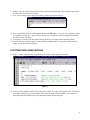
ME 104
Sensors and Actuators
Fall 2008
Laboratory 1
Introduction to LabVIEW
Department of Mechanical Engineering
University of California, Santa Barbara
Fall 2008
INTRODUCTION
In this laboratory, you will learn how to use the LabVIEW development environment, which is
based on the graphical programming language G. You will then write a LabVIEW program to acquire,
display, and save an external voltage signal.
LabVIEW is a programming language just like other programming languages, such as C, Basic, or
Pascal, but LabVIEW is higher–level. In text-based programming languages, you are as concerned about
the code as you are about what you are trying to do; you must pay close attention to the syntax (commas,
periods, semicolons, square brackets, curly brackets, round brackets, etc.). LabVIEW is much more userfriendly — it uses icons to represent subroutines, and you wire these icons together in order to define the
flow of data through your program. It is sort of like flow-charting your code as you are writing it—and the
net effect is that you can write your program in a lot less time than if you did it in a text-based
programming language. 1
LabVIEW software and hardware (data acquisition boards) have been installed on the PC’s in the
Undergraduate Control Laboratory (Engineering 2, Room 2218). To launch LabVIEW, go to the
Windows NT Start menu and proceed as follows:
Start >> Programs >> National Instruments LabVIEW 7.1
or
Start >> Programs >> National Instruments >> LabVIEW 7.1 >>LabVIEW.
LabVIEW software (without data acquisition hardware) is also available in the CADLab (Room 2243).
PART 1. INTRODUCTION TO LABVIEW 7
Objective
•
Become familiar with the LabVIEW environment.
•
Learn the general approach to building a virtual instrument in LabVIEW.
•
Build a LabVIEW virtual instrument.
Your TA will give an introductory presentation on LabVIEW 7. You will build some simple VIs to
become familiar with LabVIEW
1
Paragraph excerpts from LabVIEW—Proven Productivity (April 2000), National Instruments Corporation.
2
PART 2. USING LABVIEW WITH DATA ACQUISITION HARDWARE
Objective
•
To use a VI to acquire an analog voltage via a DAQ(data acquisition) board, plot the voltage to a
chart, and write the voltage to a spreadsheet file.
•
Review the operation of the oscilloscope and the function generator.
Experiment 2A. Acquire Analog Input Voltage
The hardware configuration for sampling an analog voltage signal is shown in Figure 1. To view a
specific analog input, you will connect an external voltage signal to the CB-68LP connector block shown
in Figure 2. The connector block is directly connected to the DAQ (data acquisition) board by a 2 meter,
shielded I/O (input/output) cable. The Tektronix CFG280 Function Generator is used to generate an
external voltage signal, which should be verified on the oscilloscope before connecting to the connector
block.
PC
DAQ board
Connector block
External voltage
Oscilloscope
Figure 1. Hardware configuration for sampling analog voltage signal.
3
Figure 2. CB-68LP connector block
•
Safety note: Before you connect an external voltage signal to the connector block, you should always
use an oscilloscope to verify that your external voltage signal is well-behaved and has an amplitude of
not more than 10 volts. Since the DAQ board is rated for voltages between –10 V and +10 V,
application of a voltage outside that range could cause irreparable damage to the (expensive) DAQ
circuitry. If you need help using your function generator or oscilloscope, please ask a TA for
assistance.
1. Using a BNC connector (Fig. on right) and cable, connect the MAIN
OUT terminal on the function generator to your oscilloscope.
2. Turn on the oscilloscope and set its vertical scale to 1.00 volts/division
and its horizontal scale to 1.00 seconds/division.
3. On your function generator, select the “MAIN 0-2Vp-p” setting by pressing down that button. This
will limit your voltage output to 2 volts, peak-to-peak 1 .
4. Find the FUNCTION selection buttons on your function generator. Select (press down) the sine wave
function (◠◡) button. Make sure that none of the other buttons on that row are pressed down.
5. Turn ON the function generator.
6. Press the down MULTIPLIER ( ∇ ) button until the MULTIPLIER indicator (red light) shows 1 and
the PERIOD indictor shows SEC. In this setting, the digital display shows the output period in
seconds.
7. Turn the FREQUENCY dial on the function generator until the digital display shows approximately
1.000. This indicates that the function generator is generating a signal with a period of approximately
1 second (and therefore, a frequency of approximately 1 Hz).
1
Therefore, the maximum amplitude will be 1 V.
4
8. Find the AMPLITUDE knob on the function generator. Turn it clockwise as far as you can to select
the maximum (MAX) amplitude of 2V peak-to-peak.
9. Verify on your oscilloscope that the output from your function generator is, in fact, a sine wave with
an amplitude of 1 volt and a period of 1 second (frequency of 1 Hz). For safety purposes, please
show your output signal to a TA before proceeding to the next step.
10. Connect the analog voltage and analog ground from your function generator to the CB-68LP connector
block as shown in Table 1. You should use wires with stripped ends 1 to make the indicated
connections. Do not remove the connections to the oscilloscope.
Table 1: CB-68LP connector block pin assignments for measuring a voltage signal using Analog Input
Channel 0.
External Signal (from Function Generator) Connect to:
Analog voltage (Red probe)
Pin 68 (ACH0)
Analog ground (Black probe)
Pin 67 2 (AIGND)
You are now ready to run your VI.
11. Go to the front panel and run the VI. Your Analog Input Chart should display a voltage signal that
appears somewhat distorted due to graphical interpolation effects.
12. When you click on the Stop button, a dialog box will appear as before. Type
yourname_lab1_SineWav.txt and Save this to your ECI account. This (long) name indicates
that the data you saved is from Lab #1, Experiment #2A, in which you sampled a 1 Hz signal every
250 milliseconds.
13. Disconnect your function generator from the CB-68LP connector block.
SAVING FILES
Before you leave, make sure all of your files are saved to your ECI account or to a floppy disk
(for later use and backup purposes). For this laboratory, you should save the following files:
yourname_lab1_TempConvert.vi
yourname_lab1_UsingLoops.vi
yourname_lab1_DAQ.vi
yourname_lab1_FileIO.vi
1
After inserting the wires, use your screwdriver to tighten the connection.
2
In addition to pin 67, pin numbers 64, 59, 56, 24, 27, 29, and 32 can also be used for specifying analog input ground
(AIGND). In practice, however, it is best to use the AIGND pin that is closest to the analog input.
5
Also save the following text files for later use:
yourname_lab1_SineWav.txt
LABORATORY REPORT
For each of the VI’s you wrote in this laboratory (listed in the preceding section), provide a printout that shows the
front panel and block diagram. Instructions for obtaining these printouts are provided in the Laboratory #1
Supplemental Handout. 1
1. (70 Points) Print out a tiled version of the front panel and block diagram for each of the four VI’s
saved to your account (listed above). Be sure to capture relevant data in the Front Panel window.
What’s the difference between a chart and a graph?
2. (20 Points) Using your favorite graphing program (such as Matlab or MS Excel), plot your voltage
data from the yourname_lab1_ex2a_SineWav.txt file. Hints for plotting this data are
provided in the Laboratory #1 Supplemental Handout. Comment on the appearance of your data
plot. If you sample a 1Hz sinewave at one sample per second, will you be able to reconstruct the
signal? This relates to the issue of aliasing to be discussed later in the lecture.
Your Lab Report should clearly state your name, Lab Report number (#1 in this case), Lab date, and
your laboratory partner’s name (if any). Only turn in ONE REPORT per team. Your lab report should be
thorough, but concise. You will be graded on quality, not quantity. Lab Report #1 is due at the
beginning of Laboratory #2.
ADDITIONAL READING AND PRACTICE
LabVIEW manuals are available online.
1. Getting Started with LabVIEW. Read this to learn about online help.
2. LabVIEW User Manual Feel free to browse through this to explore the programming resources
available in LabVIEW. Available online at http://www.ni.com.
3. If you would like to learn more about the PCI-6024E DAQ Board, you can find its DAQ
Specifications at www.ni.com/catalog/pdf/1mhw327_28,344_48,312_13a.pdf.
4. Feel free to experiment with LabVIEW programming in the CADLab. Doing so is an excellent way to
reinforce and expand on the material you learned in today’s laboratory.
1
This will be handed out during Laboratory #1.
6
ME 104 - Fall 2008
Laboratory #1 Supplemental Handout
Although this handout is intended for students using MS Word and Matlab (Version 6.0 or higher),
feel free to use a word processor and a graphing program of your choice.
•
•
To capture only the active window:
o Select the window
o <Alt><PrintScrn>
To capture the entire screen:
o <PrintScrn>
PRINTING FRONT PANEL AND BLOCK DIAGRAM OF A LABVIEW VI
USING MS WORD
1.
2.
3.
4.
5.
6.
Launch LabVIEW and open the VI you would like to print.
Select Tile Left and Right from the Window menu.
Hit <PrintScrn> on your keyboard.
Open an MS Word document (presumably, your lab report).
Select Paste from the Edit menu. The front panel and block diagram of your VI should appear.
You can adjust the size of your picture by clicking on it and selecting the Crop option from the
Picture toolbar.
7. You can add a caption to your picture by clicking on the picture and selecting Caption from the Insert
menu.
COPYING DATA FROM A TEXT FILE TO A MATLAB M-FILE USING
NOTEPAD
1.
2.
3.
4.
Launch Notepad and open the text file ( *.txt ) that contains the data you wish to view.
Select Select All from the Edit menu. All the data should be highlighted.
Select Copy from the Edit menu.
Launch Matlab and select the working directory (location) to which you would like to save your
Matlab files. You can do this by clicking on the Browse for Folder (...) button to the right of the
Current Directory listing (top menu).
5. Go to the Matlab Command Window and type cd at the command prompt (>>) to verify your
working directory.
6. Select New>>M-file from the File menu. A Matlab editor window will appear with an Untitled mfile.
7. Click on the Untitled m-file and select Paste from the Edit menu. The data that you copied from your
Notepad document should appear as a long row (Figure 1). Data points will be separated by spaces.
7
Figure 1
8. Enclose your row data by inserting a left square bracket at the beginning of the data and a right square
bracket on the line below the row data.
9. Give your row data vector a name (for example, signal) as shown in Figure 2.
Figure 2
10. Save your Untitled m-file by selecting Save As from the File menu. Give your file a descriptive name
(for example, me104_lab1). After you save the file, the .m extension will be automatically added at
the end of your m-file name.
11. Verify that your m-file is in the current working directory by typing ls at the command prompt.
12. You can run your m-file by typing its name at the command prompt. If you run the m-file shown in
Figure 2, your data will be displayed.
PLOTTING DATA USING MATLAB
13. Figure 3 shows a sample m-file for plotting a row-vector (such as signal) versus time.
Figure 3
14. You may find commands such as whos, title, xlabel, ylabel, axis, grid, and subplot useful. To find out
about these commands, you can type help followed by the name of the command. For example, to
learn about the plot command, go to the command prompt and type help plot.
8