Download School of Physics Experiment 2. Data Acquisition with Computers

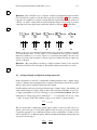
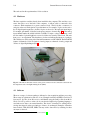
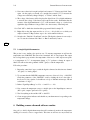
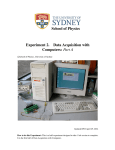
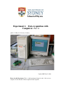
School of Physics
Experiment 2. Data Acquisition with
Computers: Part A
c
School
of Physics, University of Sydney
Updated BWJ July 23, 2014
How to do this Experiment: This is a half-experiment designed to take 1 lab session to
complete. It is the first half of Data Acquisition with Computers.
2–2
1
S ENIOR P HYSICS L ABORATORY
Safety First
This experiment uses mains-powered equipment. If you suspect an item of equipment is
not operating correctly, turn it off and turn off the power at the mains switch, then consult a
tutor. Otherwise, there are no particular safety issues with this experiment.
2
Objectives
Computers are used extensively in modern physics to control instrumentation, and to record
and process data. The purpose of this Experiment is to introduce the basic concepts of
data acquisition and digitization using computers. The technical skills needed to automatically control and acquire data using a computer are essential attributes for the experimental
physicist.
3
Background Reading and Pre-work
This Experiment makes use of basic principles of electronics and circuit analysis. It builds
on concepts such as analog to digital converters, comparator circuits, binary to decimal
conversion and logic operations. The student is strongly encouraged to complete the prework questions before attending the Laboratory. The answers can be obtained by making
use of numerous resources available on the web and in any standard textbook on electronics
(for instance, those available at the front of the Senior Lab).
4
Introduction
Almost all laboratory experiments use computers to record their results. In the past, the
recording could have been done by many methods such as chart records, xy-plotters, oscilloscopes, or simply by eye and using pen and paper. But with technological sophistication
and the need for larger data sets, there is a need to transfer readings into a computer for ease
of data manipulation or communication. The method of transferring data into a computer
in real-time is known as data acquisition (sometimes abbreviated DAQ). For an overview of
data acquisition click on the link:
http://sine.ni.com/np/app/culdesac/p/ap/daq/lang/en/pg/1/sn/n17:daq/docid/tut-8734
There are many different approaches to acquiring data with a computer. The simplest incarnations make use of “sound cards” to digitize analog voltage signals from a microphone
or instrument. An example of such an instrument would be a photo detector that generates
a voltage proportional to the light intensity. A key aspect of computer interfacing is the
analog to digital converter. This is usually an electronic circuit, although continuous (analog) information can also be digitized using other means. Computers process information
as binary numbers (1 and 0, or ON and OFF) using Boolean algebra.
Question 1: [Pre-work] How can base-10 numbers (decimal) be converted to base-2 (binary)? Convert the number 15 to binary.
DATA ACQUISITION WITH C OMPUTERS : Part A
2–3
C1 .
Question 2: [Pre-work] How does a computer compute by manipulating binary information? Describe the operation of the Boolean logic gates in the Figure 2-1. How can these
logic gates be assembled to construct a circuit that performs the mathematical operation of
addition - an “adder” circuit? Draw an adder circuit that adds two binary digits to produce
a sum digit and a carry digit. Draw a truth table (like those in Figure 2-1) for the adder.
C2 .
Fig. 2-1 : Some logic gates with their truth tables that show the output states depending on the input
(a) A AND B must both be 1 for the output to be 1 (b) NAND is the exact opposite of AND (c)
OR means A OR B have to be 1 for the output to be 1 (d) Exclusive OR (XOR) is the same as the
OR gate except that if both A and B are 1, then the output is 0 (e) NOT means that the output is the
opposite to the input.
Question 3: [Pre-work] What is an analog to digital converter? Draw a basic electronic
circuit that could be used for this purpose and explain in bullet point form how it works.
C3 .
4.1
Analog to digital and digital to analog conversion
In this experiment you will use a commercially available interface card to digitize analog
voltages so that they can be manipulated by a computer. The interface card can also produce
analog voltages based on digital signals from the computer.
Usually, interface cards can only accept a limited range of input voltages, and similarly, can
output a limited range of voltages. Suppose that a card can accept a maximum of ±10 Volts,
or output a maximum of ±10 Volts, and suppose our card had 8 bit resolution. The 8-bit
means that our voltage range can be divided into 28 = 256 equal parts. In our case, -10 V
→ +10 V is a range of 20 V. The smallest voltage we can obtain or output is given by
20 V
' 78 mV
256
This also means that a continuously varying signal (such as a sine wave) will only be acquired or sent out in steps of 78 mV. This might look like it’s pretty good, but an 8 bit card
is generally regarded as not of sufficient resolution for most experiments. Usually a 12 bit
card is regarded to be of sufficient quality. This means that the maximum voltage range can
only be resolved in steps of
range
range
=
212
4096
2–4
S ENIOR P HYSICS L ABORATORY
The card used in this experiment has 12 bit resolution.
4.2
Hardware
The data acquisition card has already been installed in the computer. This card has a connector that pokes out of the back of the computer. A ribbon cable is connected to this
connector, which terminates in a green connector block. This block has a connector for
each pin on the card. Each pin has a specific function. For example, 32 pins are devoted to
the 32 digital input/output lines. Another 16 pins are devoted to the analogue input/output.
For example, pin number 3 (labelled on the green connector, shown in Fig. 2-2) is the analog
input channel number 0, usually labelled as ACH0. To input a voltage we connect a wire
into the number 3 pin and tighten its screw to hold the wire securely in the block. The wire
then goes to our experiment. The bench notes for the card indicate the function of each pin.
The card that we will be using is the National Instruments card PCI-6025E. The PCI-6025E
features 16 channels (12 bits resolution) of analog input, two channels of analog output and
32 lines of digital Input/Output (I/O).1
Fig. 2-2 : The ribbon cable that connects to the green connector block. Connected to this block are
the temperature sensor and light emitting diodes (LED)
4.3
Software
There are a range of software packages dedicated to data acquisition and data processing.
These range in sophistication and ease of use. Examples include LabVIEW from National
Instruments, Igor Pro from Wavemetrics and Matlab using the DAQ toolkit from MathWorks. It is also possible to write code in your favorite high-level programing language to
send and receive data to an external interface. The choice of interface for sending and receiving data depends on the speed and type of data to be exchanged. Examples of interface
buses include: USB, PCI, PXI, GPIB. You may wish to learn more by searching for these
acronyms on the web.
1
More information about the PCI-6025E can be found in [1]
DATA ACQUISITION WITH C OMPUTERS : Part A
2–5
Throughout this experiment you will be acquiring and outputting data using the LabVIEWTM
software, which is a product of the National Instruments company. It is one of the more popular programming environments for computer interfacing because it is an icon based programming language. That is, you program by dragging the appropriate icons onto the screen
and connecting lines between them. This experiment is about learning to use LabVIEWTM
and interface cards. We will be using version 8 of LabVIEWTM to carry out computer
interfacing to experiment.
5
Getting started with LabVIEW
Our goal is to build a simple voltmeter and a simple digital thermometer using the temperature sensor LM35DZ.
At all stages of this practical you should print out key windows from LabVIEW and
stick them in your logbook. In addition, you should add comments to explain how the
software works.
5.1
A simple voltmeter
We want to be able to apply a voltage to the connector block and have the computer display
its value on the screen. The following procedure will show you how to do this.
1. Double click on the “National Instruments LabVIEW 8.0” icon on the desktop to
open the “Getting Started” window.
2. Click on “VI from Template...” and choose:
Create N ew → V I → DAQ → Data Acquisition with N I − DAQmx.vi.
The windows “Untitled 1 Block Diagram” and “Untilted 1 Front Panel” will be created.
3. Follow the instructions in the yellow box in the “Untitled 1 Block Diagram” window
to create an “Analog Input” measurement.
4. In the “Create New Express Task...” window choose Analog Input → V oltage.
5. Select the “ai0” input from “Dev1 (PCI-6025E)” and click the “Finish” button.
6. The “DAQ Assistant” will open and enable you to configure the “Voltage Input”. In
the “Terminal Configuration” list box choose “RSE”2 . This is a mode3 where measured voltage is applied between ground (AIGND pin1 or pin2) and channel 0 analog
input (ACH0 pin3). Hit the “Test” button to test your analog input configuration.
7. A new “DAQ Assistant” window will open. Connect analog input to the ground, by
connecting pin1 and pin3 using a piece of wire, and hit the “Start” button. You should
see a horizontal straight line at 0 Volts with some 2.4 mV “spikes”.
Question 4: Explain the origin of the 2.4 mV spikes.
2
3
Reference Single Ended
There are two other input modes: differential and non-reference single ended.
2–6
S ENIOR P HYSICS L ABORATORY
8. Now remove the wire from pin1 and pin3 and connect 1.5 V battery and click “Start”
again. On the graph you should see a straight line around 1.5 V. To measure the
voltage more accurately change “Display” to “Values” and hit “Start”.
9. The voltage of the battery will be displayed in digital form. Use a digital multimeter
to measure the voltage of the battery and compare the results. Remember that the
accuracy of the digital multimeter is ±1% of the measured voltage or ±1 at the least
significant digit, whichever is larger. This is also the accuracy of the DAQ card.
10. Click “OK” to finish the wizard and the program will build a simple VI.
11. Right click on the data output and choose: Create → Graph Indicator to finish your
simple voltmeter VI. Repeat these steps to also add a numeric indicator.
12. Switch to the “Untitled 1 Front Panel” window. The digital voltmeter is now ready to
use. To start the voltmeter click “Run” or “Run Continuously” button.
C4 .
5.2
A simple digital thermometer
This project is very similar to the previous one. To measure temperature we will use the
temperature sensor LM35DZ. This sensor has 3 terminals: 0 V, +5 V and output. The output
has a voltage that is proportional to the temperature of the sensor. A 0 V output corresponds
to a temperature of 0◦ C. A temperature change of 1◦ C produces a change in output of
10 mV. We will use the analog channel “ACH1” (pin5) to read the temperature.
Follow the procedure:
1. Repeat the same first 6 steps as with the digital voltmeter, but this time use channel
“ai1 (pin5)” as “Analog Input”.
2. To accommodate the LM35DZ temperature sensor use Custom Scaling → LM35DZ.
Check the parameters of the “LM35DZ” scale by clicking the icon to the right of
the Custom Scaling window. It should have a slope of 100 and an intercept of 0 and
scaled units of “deg C”.
3. Define “Signal Input Range” as M in = 0 and M ax = 100.
4. Now connect the temperature sensor to suitable pins on the Input/Output connector
(0 V to pin1, output to pin5 and +5 V to pin35).
5. Test if everything works and hit “OK” to build VI.
6. Create an appropriate indicator and check how your thermometer is responding to the
temperature change.
6
Building a more advanced software routine
Our goal is to build a digital thermometer that will continuously monitor the temperature
and flag if it exceeds a lower or upper limit. This time we will not use any wizard, but
DATA ACQUISITION WITH C OMPUTERS : Part A
2–7
start from scratch with a new empty VI. A schematic of your project is shown in Fig. 2-3.
For your convenience we collected all the components needed to build this VI in “ThermometerComponents.vi”. You can copy any component from this file and place it in your
project, but also you can use the “Function palette” that is built into LabVIEW to get other
components to enhance your VI.
Fig. 2-3 : Block Diagram of the Advanced Thermometer.
The Front Panel for this project is shown at Fig. 2-4. You are welcome to modify this front
panel to make it more functional and clear for the user.
Fig. 2-4 : Front Panel of the Advanced Thermometer.
We will not give you a step-by-step description on how to build your project. Below are just
a few hints:
• Analyse the schematic of the Advanced Thermometer and try to distinguish a few
different functional groups of this VI.
• Build your project in steps and test frequently.
• To get help on any component, select it and press Ctrl +H. If you are still a beginner
in LabVIEW programming, use this option on every component which you use in
your project.
2–8
S ENIOR P HYSICS L ABORATORY
• LabVIEW comes with a lot of examples and help files.4 Use them!
• The lower part of the schematic allows us to connect the external LED indicators.
Analyse it carefully before you physically connect wires (by default black wire should
be connected to the digital ground DGND pin 33 and other to digital outputs: DIO0
pin 25, DIO1 pin 27 and DIO2 pin 29).
C5 .
References
[1] DAQ 6023E/6024E/6025E User Manual. National Instruments.
[2] DAQ NI-DAQ User Manual for PC Compatibles. National Instruments.
[3] National Instruments LabVIEW User Manual. National Instruments.
4
Good introduction to LabVIEW can be found in [2, 3].