Download implementation of pid controller for controlling the liquid level of the

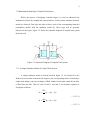
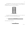
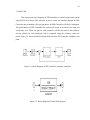
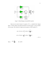
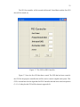
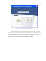
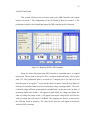
IMPLEMENTATION OF PID CONTROLLER FOR
CONTROLLING THE LIQUID LEVEL OF THE COUPLED
TANK SYSTEM
MOHD IZZAT B DZOLKAFLE
EC 05042
UNIVERSITI MALAYSIA PAHANG
v
ABSTRACT
The PID controllers have found wide acceptance and applications in the
industries for the past few decades. In spite of their simple structures, PID controllers are
proven to be sufficient for many practical control problems. This project presents the
PID controller design for controlling liquid level of coupled tank system. These coupled
tank liquid level systems are in second order system. The PID Controller will be
designed to control the liquid level at tank 1 and design techniques of the PID Controller
are then conducted based on developed model. MATLAB has been used to simulate and
verified the mathematical model of the controller. Visual Basic 6 has been used to
implement the graphical user interface (GUI) and implementation issues for the
controller’s algorithms will also be discussed. The DAQ card is used for interfacing
between hardware and software. The simulated result will be compared with the
implemented result.
xiii
LIST OF FIGURE
FIGURE
TITLE
1.1
Block Diagram of the coupled tank control apparatus
1
3.1
Flow chart for software and hardware development
7
3.2
Schematic Diagram of coupled tank system
9
3.3
Block Diagram of Second Order Process
17
3.4
Block Diagram of PID Controller combines with plant
20
3.5
Block Diagram of inside plant system
20
3.6
Block Diagram of inside PID Controller
21
3.7
The GUI for PID Controller
23
3.8
The GUI for DAQ card detection
24
3.9
The GUI for software controller
25
3.10
The GUI for Data Collected
26
3.11
Advantech DAQ card connection
27
PAGE
xiv
4.1
Coupled Tank without controller
28
4.2
Step Source Block Parameter
29
4.3
Coupled Tank Function Block Parameter
29
4.4
Plot of Liquid Level at the Coupled Tank 1
30
4.5
Plot performance of Proportional Controller
31
4.6
Plot performance of Proportional-Derivative Controller
32
4.7
Plot performance of Proportional-Integral Controller
33
4.8
Plot performance of PID Controller
34
4.9
Result at GUI for PID Controller
35
4.10
Output for Tank 1
36
vii
TABLE OF CONTENTS
CHAPTER
CONTENTS
PAGE
TITLE
i
DECLARATION
ii
DEDICATION
iii
ACKNOWLEDGEMENT
iv
ABSTRACT
v
ABSTRAK
vi
TABLE OF CONTENTS
vii
LIST OF FIGURES
xiii
LIST OF TABLES
xv
LIST OF ABBREVIATIONS
xvi
LIST OF APPENDICES
xvii
x
1
INTRODUCTION
1
1.1
Overview
1
1.2
Problem Statement
2
1.3
Objective
3
1.4
Scope of Project
3
1.5
Summary
3
LITERATURE REVIEW
4
2.1
Overview
4
2.2
Article
4
2.3
Summary
5
METHODOLOGY
6
3.1
Overview
6
3.2
Project Flow Chart
7
3.3
Mathematical Modeling of Coupled Tank System
9
3.3.1
9
2
3
A Simple Nonlinear Model of
Coupled Tank System
3.3.2
A Linearised Perturbation Model
11
3.3.3
First Order Single Input Single Output (SISO)
13
Plant
xi
3.3.4
Second Order Single Input Single Output
15
(SISO) Plant
3.4
Controller Design
18
3.5
MATLAB
20
3.6
Microsoft Visual Basic
22
3.7
DAQ card
27
3.8
Summary
27
RESULT, ANALYSIS AND DISCUSSION
28
4.1
Overview
28
4.2
Simulation Result without Controller
28
4.3
Simulation Result with PID Controller
31
4.4
Real Time Result
35
4.5
Discussion for PID Controller
37
4.6
Comparison between simulation and
37
4
Implementation result
4.7
Summary
38
xii
5
CONCLUSION AND FUTURE
39
RECOMMENDATION
5.1
Conclusion
39
5.2
Future Recommendation
40
5.3
Costing and commercialization
41
REFERENCE
42
APPENDIX A
43
APPENDIX B
44
APPENDIX C
45
APPENDIX D
52
APPENDIX E
57
APPENDIX F
58
xvii
LIST OF APPENDICES
APPENDIX
TITLE
A
M-file coding
43
B
First GUI coding
44
C
Second GUI coding
45
D
Third GUI coding
52
D
Fourth GUI coding
57
D
DAQ card Datasheet
58
PAGE
xvi
LIST OF ABBREVIATIONS
PID
-
Proportional-Integral-Derivative
DAQ
-
Data acquisition
GUI
-
Graphic User Interface
CTS-001
-
Coupled Tank Liquid Level System
SISO
-
Single Input Single Output
PV
-
Process Variable
MV
-
Manipulative Variable
SP
-
Set Point
V
-
Voltage
USB
-
Universal Serial Bus
Kp
-
Proportional Gain
Ki
-
Integral Gain
Kd
-
Derivative Gain
RC
-
Resistor-Capacitor Circuit
1
CHAPTER 1
INTRODUCTION
1.1 Overview
Industrial application of liquid level control abound, such as in food processing,
nuclear power generation plant, industrial chemical processing and pharmaceutical
industries. The typical actuators used in coupled tank liquid level system include of two
small tanks mounted above a reservoir which functions as storage for the water [4]. Each
of both small tanks has independent pumps to pump water into the top of each tank [4].
At the base of each tank have a flow valve connected to reservoir. In addition, level
sensors such as capacitive-type probe to monitor the level of water in each tank,
displacement float and pressure sensor provide liquid level measurement [4].
The PID Controller usually used for temperature, motion and flow controllers. It’s
available in analog and digital forms. PID Controller will control the water pump so that
water in both tank in level as required. The DAQ card is used as the interface to connect
the system and equipment. Software such as MATLAB will be used to get the simulation
result of the system performance and Microsoft Visual Basic 6 to implement the designed
controller by developing Graphical User Interface (GUI). Figure 1.1 shows the block
diagram of the coupled tank control apparatus with controller.
Figure 1.1: Block diagram of the couple-tank control apparatus.
2
1.2 Problem Statement
The Proportional-plus-Integral-plus-Derivative (PID) controllers have found wide
acceptance and applications in the industries for the past few decades. It has a simple
control structure which was understood by plant operators and which they found
relatively easy to tune. In spite of the simple structures, PID controllers are proven to be
sufficient for many practical control problems and hence are particularly appealing to
practicing engineers. An abundant amount of research work has been reported in the past
on the tuning of PID controllers. Ziegler Nichols step response, Ziegler Nichols ultimate
cycling, Cohen Coon, Internal model control, and error-integral criteria tuning formulae
are to mention only a few [7]. "PID" means Proportional-Integral-Derivative, referring to
the three terms operating on the error signal to produce a control signal. Since many
control systems using PID control have proved satisfactory, it still has a wide range of
applications in industrial control.
In this project, several useful PID Controller design techniques will be presented,
and implementation issues for the algorithms will also be discussed. The PID Controller
will be designed to control the liquid level at tank 1. In this project, the simulation of
proportional, integral and derivative actions are explained in detail, and variations of the
basic PID structure are also introduced. A graphical user interface (GUI) implementing of
PID Controller tuning formulae will also be present at this project.
Finally, we need continuous data from the plant as the feedback, so to overcome
this problem an Advantech DAQ card have been used as the interfacing device between
the hardware and software.
3
1.3 Objective
There are several objectives that must be achieved in order to make this project
successful;
i.
To develop a PID Controller for controlling the liquid level of tank one of coupled
tank system.
ii.
To validate the result from simulation (using MATLAB) through experimental set
up (implementation using Microsoft Visual Basic 6).
1.4 Scope of project
This project is all about how to designed the controller and simulate it using
MATLAB. Then, implement PID Controller by developing GUI using Microsoft Visual
Basic 6 software on coupled tank liquid level system. After that, both results are
compared.
There are several software will be used, first software is MATLAB 7.1 that been
used to simulate and verified the mathematical model of the controller. Second software
that will be us is Microsoft Visual Basic 6 that been used to implement the graphical user
interface for PID Controller.
The communication between DAQ card, Visual Basic 6 and Coupled tank liquid
level system will be determined, in term of address to give or receive analog or digital
signal.
1.5 Summary
This chapter is about the explanation for overall project. The objective and the
scope of the project will be given in order to give an insight about the idea of the project.
On the next chapter, the literature review for this controller but use at different system
and same system but with different controller will be discussed.
4
CHAPTER 2
LITERATURE REVIEW
2.1 Overview
This chapter will discuss about the article that referred for this controller but
applied at different plant or different method to designing and also for different controller
but applied at same plant or same method of designing.
2.2 Article
[1]
Jutarut
Chaorai-ngern,
Arjin
Numsomran,
Taweepol
Suesut,
Thanit
Trisuwannawat and Vittaya Tipsuwanporn., ” PID Controller Design using
Characteristic Ratio Assignment Method for Coupled-Tank Process”, Faculty of
Engineering, King Mongkuts Institute of Technology Ladkrabang, Bangkok
10520, Thailand
This paper presents the PID controller design for coupled tank process
using characteristic ratio assignment (CRA).The simulation results can be
illustrated the validity of their approach by MATLAB
[2]
Mohd Fua’ad Rahmat and Mariam MD Ghazaly.,” Performance Comparison
between PID and Fuzzy Logic Controller in Position Control System of DC
Servomotor”, Jurnal Teknologi, 45 (D) Dis. 2006: 1-17
This paper presents the comparison between PID controller and Fuzzy
Logic Controller about their time specification performance in position control
system of a DC motor. This paper included design and development of a GUI
software using Microsoft Visual Basic 6 to programming real time software.
5
[3]
Muhammad Rehan, Fatima Tahir, Naeem Iqbal and Ghulam., ” Modelling,
Simulation and Dicentralized Control of a Nonlinear Coupled Tank Systam”,
Department of Electrical Engineering, PIEAS, Second International Conference
on Electrical Engineering 25-26 March 2008 University of Engineering and
Technology, Lahore (Pakistan)
This paper presents a coupled three tank system is taken as a plant and will
be
modeled
mathematically
using
Bernoulli’
s
law,
simulate
with
Matlab/Simulink and decentralized using control and estimation tool manager
from simulink model and mathematical model
2.3 Summary
This chapter is about the explanation for some article that will refer to gets the
information or some knowledge that will apply to make the project run successfully.
They are several articles that explain about same controller that will use in this project
but applied at different plant or different method of designing, and also different
controller but applied at same plant.
6
CHAPTER 3
METHODOLOGY
3.1 Overview
This chapter will discuss about the method that has been used to complete this
project. The coupled tank liquid level system CTS-001 will be used in this project as a
plant. In this project, several useful PID Controller design techniques will be presented.
The PID Controller will be designed to control the liquid level at tank one to obtain the
desired level. In this project, Advantech DAQ card have been used as the interfacing
between the hardware and software.
7
3.2 Project Flow Chart
Figure 3.1: Flow chart for software and hardware development
8
Figure 3.1 shows about the overall progress for both software and hardware
development that will discuss later. This project will be divided to two parts to make sure
this project run smoothly. The first part is a software part, which will cover modeling the
controller. The controller must be designed and simulated using MATLAB and then
implemented in Visual Basic 6 as GUI. The second part will cover for the hardware part.
In this part, the coupled tank liquid level system will be assembled to make sure it will
run properly. Then, a communication between plant and controller must be done using
DAQ card. The DAQ card must be analyzed and these operations need to refer the
manual, to make the interfacing between plant and controller.
After that, both parts must be integrated to test the whole system. At this part, the
real time result that implemented using Visual Basic 6 must be compared with the
experiment result that simulated using MATLAB. Troubleshooting will be performed if
some errors occurred to obtain better result.
9
3.3 Mathematical Modeling of Coupled Tank System
Before the process of designing controller begin, it is vital to understand the
mathematics of how the coupled tank system behaves. In this system, nonlinear dynamic
model are observed. Four steps are taken to derive each of the corresponding linearised
perturbation models from the nonlinear model [4]. These steps will be generally
discussed in this topic. Figure 3.2 shows the schematic diagram of coupled tank system
that been used.
Figure 3.2: Schematic Diagram of Coupled Tank System
3.3.1 A Simple Nonlinear Model of Coupled Tank System
A simple nonlinear model is derived based on figure 3.2. Let H1and H2 be the
fluid level in each tank, measured with respect to the corresponding outlet. Considering a
simple mass balance, the rate of change of fluid volume in each tank equals the net flow
of fluid into the tank. Thus for each of tank 1 and tank 2, the dynamic equation is
developed as follows.
1 1
i1 o1 o3
….. (3.3.1.2)
2 2
i2 o2 o3
….. (3.3.1.3)
10
Where
H1, H2 = height of fluid in tank 1 and tank 2 respectively
A1.A2 =cross sectional area of tank 1 and tank 2 respectively
Qo3 =flow rate of fluid between tanks
Qi1, Qi2 = pump flow rate into tank 1 and tank 2 respectively
Qo1, Qo2 = flow rate of fluid out of tank 1 and tank 2 respectively
Each outlet drain can be modeled as a simple orifice. Bernoulli’s equation for
steady, non viscous, incompressible shows that the outlet flows in each tank is
proportional to the square root of the head of water in the tank. Similarly, the flow
between the two tanks is proportional to the square root of the head differential.
o1 o2 o3 1
2
3
1
….. (3.3.1.4)
….. (3.3.1.5)
1 2
….. (3.3.1.6)
Where α1, α2, α3 are proportional constants which depend on the coefficients of
discharge, the cross sectional area of each orifice and the gravitational constant.
Combining equation (3.3.1.4), (3.3.1.5) and (3.3.1.6) into both equation (3.3.1.2) and
(3.3.1.3), a set of nonlinear state equations which describe the system dynamics of the
coupled tank are derived
1
1
i1 1
1 3
1 2
….. (3.3.1.7)
2
2
i2 2
2 3
1 2
….. (3.3.1.8)
11
3.3.2 A Linearised Perturbation Model
Suppose that for a set of inflows Qi1 and Qi2, the fluid level in the tanks is at some
steady state level H1 and H2. Consider a small variation in each inflow, q1 in Qi1 and q2 in
Qi2. Let the resulting perturbation in level be h1 and h2 respectively. From equations
(3.3.1.7) and (3.3.1.8), the equation will become:
For Tank 1
1
1 1
i1
1 1
1
1 3
1 2
1 2
….. (3.3.2.1)
For Tank 2
2
2 2
i2
2 2
2
2
3
1 2
1 2
….. (3.3.2.2)
Subtracting equations (3.3.1.7) and (3.3.1.8) from equation (3.3.2.1) and (3.3.2.2),
the equations that will be obtained are,
1
1
1 1
1
1 1 3
1 2
1 2 1 2
….. (3.3.2.3)
2
2
2 2
2
2 2
3
1 2
1 2 1 2
….. (3.3.2.4)
12
For small perturbations,
1
1
1
1 1 ….. (3.3.2.5)
Therefore,
1
1 1 2
2 2 1
1
Similarly,
2
2
And
2 1
2 1 2 1 2 1
2 1
Simplify equation (3.3.2.3) and (3.3.2.4) with these approximations will become,
1
1
1 1
1
1 3
1 2
1 2
….. (3.3.2.6)
2
2
2 2
2
2
3
1 2
1 2
….. (3.3.2.7)
13
In equations (3.3.2.6) and (3.3.2.7), note that the coefficients of the perturbations
in level are functions of the steady state operating points H1 and H2. Note that the two
equations can also be written in the form
1
1
1 o1 3
1 2
1 2
….. (3.3.2.8)
2
2
2 o2
3
2 1 2
1 2
….. (3.3.2.9)
where qo1 and qo2 represent perturbations in the outflow at the drain pipes. This would be
appropriate in the case where outflow is controlled by attaching an external clamp for
instance.
3.3.3 First Order Single Input Single Output (SISO) plant
This configuration is considered by having the baffle completely depressed so that
there is no flow between the two tanks. Equation (3.3.2.6) and (3.3.2.7) can be simplified
to become first order differential equation.
1
1
1
1 1
2 1
….. (3.3.3.1)
2
2
2
2 2
2 2
….. (3.3.3.2)
14
Taking the level of fluid at tank 1 that will control, the output variable h1
represents a small change in the steady state level H1 and q1 is a small change in the
steady state input flow rate into tank 1, Qi1. H1 is also the steady state operating points
and is a constant. Performed laplace transform on equation (3.3.3.1) will become,
1 1 2 1
1
1
21 1
1
t
1 ….. (3.3.3.3)
From equation (3.3.3.1), the time constant of the tank 1 dynamics can be expressed
1 21 1
1
….. (3.3.3.4)
The steady state gain of the tank 1 dynamics is
t 2 1
1
….. (3.3.3.5)
15
3.3.4 Second Order Single Input Single Output (SISO) plant
This configuration is considered by having the baffle raised slightly. The
manipulated variable is the perturbation to tank 1 inflow. Performed laplace transform of
equation (3.3.2.6) and (3.3.2.7), and assuming that initially all variables are at their steady
state values,
11 1(s) 2 1
1
3
2 1 2
1 3
2 1 2
2 ….. (3.3.4.1)
22 2(s) 2 2
2
3
2 1 2
2 3
2 1 2
1 ….. (3.3.4.2)
Rewritten equation (3.3.4.1) and (3.3.4.2)
1
11 11 122 ….. (3.3.4.3)
2
12 22 211 ….. (3.3.4.4)
16
Where
1=
1
1
2 1
3
2 1 2
….. (3.3.4.4)
2=
2
2
2 2
3
2 1 2
….. (3.3.4.5)
1=
1
1
2 1
3
2 1 2
….. (3.3.4.6)
2=
1
2
2 2
3
2 1 2
….. (3.3.4.7)
3
12=
1
2 1 2
2 1
3
2 1 2
….. (3.3.4.8)
3
21=
2
2 1 2
2 2
3
2 1 2
….. (3.3.4.9)
17
For the second order configuration that shows on figure 3.3, h2 is the process
variable (PV) and q1 is the manipulated variable (MV). Case will be considered when q2
is zero. Then, equation (3.3.4.3) and (3.3.4.4) will be expressed into a form that relates
between the manipulated variable, q1 and the process variable, h2 and the final transfer
function can be obtained as,
2 1
1 12
1 2 1 1221
12
2
12 2
1
1 1221
….. (3.3.4.10)
Figure 3.3: Block Diagram of Second Order Process
18
3.4 Controller Design
This topic will discuss about the designing of controller that will control level
fluid at tank 1 on coupled tank system. The purpose controller that needs to design is PID
Controller. The designing of controller are divided into two methods. First method, the
controller needed to be design and simulate using MATLAB while second method,
Microsoft Visual Basic 6 is used for implementation that will create GUI for PID
controller. So that, before the both method need to be proceed, the value for each
parameters of the equation (3.3.4.10), the equation for the second order configuration
needed to be found.
Each value of α1, α2, α3, A1, A2, H1 and H2 can be obtained from calibrate
experiments manual CTS-001 book that also been provided with this plant and those
values are:
H1 = 17
H2 = 15
α 1 = 10.78
α 2 = 11.03
α 3 = 11.03
A1 = 32
A2 = 32
Table 3.1: Parameters values
19
By solving equation (3.3.4.4), (3.3.4.5), (3.3.4.6), (3.3.4.7), (3.3.4.8) and (3.3.4.9)
with those values α1, α2, α3, A1, A2, H1 and H2, the value of T1, T2, K1, K2, K12, and K21 can
be determined. So the value of T1, T2, K1, K2, K12, and K21 are:
T1 = 6.1459
T2 = 6.0109
K1 = 0.1921
K2 = 0.1878
K12= 0.749
K21= 0.7325
Table 3.2: Parameters value
By using the value that has been obtained from T1, T2, K1, K12, K12, and K21 and
put it in equation (3.3.4.10), the value of transfer functions become:
61459
60109 2
01921 01878
61459 60109
1 0749 07325
Then, the transfer function will become,
36942 2
0036
121568
0451
….. (3.4.1)
20
3.5 MATLAB
This topic presents the designing of PID Controller to control coupled tank system
using MATLAB software. This software is used to create the simulink diagram for PID
Controller and performance for each parameter for PID Controller will also be simulated.
The performances of PID Controller are evaluated in terms of overshoot, rise time and
steady state error. Then, the gain for each parameter will also be tuned in this software
and the validity for each parameter will be compared using the reference value (set
point). Figure 3.4 shows the MATLAB simulink block for PID Controller combines with
plant.
Figure 3.4: Block Diagram of PID Controller combines with plant
Figure 3.5: Block Diagram of inside Plant System
21
Figure 3.6: Block Diagram of inside PID Controller
Based on the transfer function for equation (3.4.1), a simulink block diagram
figure 3.5 will be design as the plant that needed to be control. Figure 3.6 is the controller
for this system. This controller is design based on equation of PID Controller [7],
p!
p!
i"!
d
1
" ! i
d
!
!
….. (3.5.1)
Where
Ki =
Kp
Ti
;
Kd = KpTd
22
3.6 Microsoft Visual Basic
This topic presents the designing of PID Controller to control coupled tank system
using Microsoft Visual Basic software. This software is used for getting the implement
result for the project by develop a GUI for PID Controller. Before the GUI for PID
Controller will be programmed, algorithm for PID Controller is needed [6]. So that, to
find the algorithm the set point must be compared to the process variable to obtain the
error [6].
Error = SP– PV
Then, convert equation (3.5.1) will become,
p!##$#
p
1
1
i
!##$#%!& !##$#$'
i
d
!##$#%!& !##$#$' ( d
….. (3.6.1)
23
The GUI for controller will be created in Microsoft Visual Basic and the first GUI
that will be created are,
Figure 3.7: The GUI for PID Controller
Figure 3.7 show the first GUI that been created. The GUI that has been created is
the GUI for the purpose controller that will be used to control coupled tank system. This
GUI is created based on the algorithm for PID Controller that had been stated on equation
(3.6.1). Coding for this GUI will be shown in appendix B.
24
Figure 3.8: The GUI for DAQ card detection
Figure 3.8 shows the second GUI that been created. This GUI is the first GUI that
will run if the program started. This GUI is created to detect the DAQ card that been
used. The Run button will appear after GUI detects the DAQ card and must be clicked to
proceed to next step. Coding for this GUI will be shown in appendix C.
25
Figure 3.9: The GUI for Software Controller
Figure 3.9 shows the third GUI that been created. This GUI will appear after the
second GUI by clicking the Run button at second GUI. This GUI will make the controller
start to run by clicking the Start button. Before start the process, the desired value for set
point must be inserted. In this GUI, the value for set point is setting in percentage. The
voltage range for couple tank is 0V-5V dc analog voltage. So that, 5V is equal with 100%
and so on. Coding for this GUI will be shown in appendix D.
26
Figure 3.10: The GUI for Data Collected
Figure 3.10 shows the last GUI that been created. This GUI will appear if user
clicks the Enter Data button at the third GUI. In this GUI, the data input (PV) and output
(MV) that have been collect during controller running will appear. Coding for this GUI
will be shown in appendix E.
27
3.7 DAQ Card
The DAQ Advantech 4716 will be used as the data acquisition input output card
for the real time implementation. Figure 3.11 shows the DAQ card will be function to
communicate between controller and plant.
Figure 3.11: Advantech DAQ card connection
The controller that is design will send the required signal to control pump at
coupled tank. This signal can’t be send directly to couple tank because there are no USB
connection at coupled tank. This signal must flow through into the DAQ card. Then, the
DAQ card will send this signal to coupled tank. The couple tank which consists of sensor
and actuator will react in a feedback loop and send back the information signal to
controller for next iteration. The same process will happened but in opposite direction.
The details about this DAQ card will be shown in appendix F.
3.8 Summary
This section gave an overview about the entire necessary thing that involved in
this project. The coupled tank, software and hardware related also had been discussed in
terms of it characteristics and it important parameter.
28
CHAPTER 4
RESULT, ANALYSIS AND DISCUSSION
4.1 Overview
This chapter presents the simulation and implementation result using PID
Controller for the coupled tank system. The performances for each parameter of PID
Controller are evaluated based on rise time, overshoot and steady state error. The
comparison between two results will also be discussed in this chapter.
4.2 Simulation result without controller
This section will show the simulation result without the controller. The equation
for coupled tank system will refer the equation (3.4.1). Figure 4.1 shows the coupled tank
system simulink model without controller. The step source block parameter those shown
in figure 4.2 represent the set point and figure 4.3 shows plant model function block
parameter for coupled tank system. MATLAB M-file has been used and is stated in
appendix A.
Figure 4.1: Coupled Tank without Controller
29
Figure 4.2: Step Source Block Parameter
Figure 4.3: Coupled Tank Function Block Parameter
30
Figure 4.4: Plot of Liquid Level at The Coupled Tank 1
From the figure 4.4, the liquid will constantly overflow. This situation happen
because of this system running without controller to control the Pump 1 speed, so the
Pump 1 will continuously pump the liquid out from the tank until it overflow. PID
controller must be put as it controller element so that the liquid will not overflow and will
indicates as required.
31
4.3 Simulation result with PID Controller
This section will show the simulation result with the PID Controller. The
configuration of the MATLAB simulink model for PID Controller combines with
coupled tank is shown as in figure 3.4. The performance result for each parameter are
also been discussed based on overshoot, rise time and steady state error.
Figure 4.5: Plot Performance of Proportional Controller
Figure 4.5 shows the performance of proportional controller. The set point is set
equal to 3 and the proportional gain is set 20. The plot shows that proportional controller
reduced both the rise time and the steady state error. Proportional controller also
increased the overshoot and decreased the settling time by small amount.
32
Figure 4.6: Plot Performance of Proportional-Derivative Controller
Figure 4.6 shows the performance of proportional-derivative controller. The set
point is set equal to 3. The proportional gain is set equal to 20 and derivative gain is set
equal to 10. This plot shows that the derivative controller reduced both the overshoot and
the settling time but had small effect on the rise time and the steady state error.
33
Figure 4.7: Plot Performance of Proportional-Integral Controller
Figure 4.7 shows the performance of proportional-integral controller. The set
point is set equal to 1. The proportional gain is set equal to 20 and integral gain is set
equal to 12. The plot shows that integral controller also reduced the rise time increased
the overshoot same as the proportional controller does. The integral controller also
eliminated the steady state error.
34
Figure 4.8: Plot Performance of PID Controller
Figure 4.8 shows the performance of PID Controller. The set point is set equal to
3. The proportional gain is set equal to 12, integral gain is set equal to 4 and derivative
gain is set equal to 7 to provide the desired response. The plot shows that the output
voltage achieves the set point voltage at time equal to 10 second. The output voltage have
slightly overshoot before stabilize at time equal to 20 second.
35
4.4 Real Time Result
This section will shows the real time result as the PID Controller will control
liquid level at tank 1. The configuration of the GUI model is shown at section 3.6. The
performance result for level liquid that control by PID Controller will be discussed.
Figure 4.9: Result at GUI for PID Controller
Figure 4.9 shows the result when PID Controller is controlled tank 1 at coupled
tank system. The set point is set equal to 50%. As that be mentioned before, 50% is equal
with 2.5V. The proportional gain is set equal to 12, integral gain is set equal to 4 and
derivative gain is set equal to 7 to provide the desired response. After the Start button is
clicking, the controller starts to run and send desired voltage to pump at tank 1. The value
of desired voltage will state at manipulative variable block. At the same time, the flow of
increasing liquid level at tank 1 will appear at graph block. At voltage read block, the
value of voltage for pump at tank 1 will appear and output voltage block will state the
value of voltage that will send as a feedback. The sampling rate block is a real time for
this GUI that stated in frequency. The value for PV and error will appear at data block
when this GUI is running.
36
Figure 4.10: Output for Tank 1
Figure 4.10 shows plot that will appeared when the system are running. The
output voltage did not achieve the set point voltage that is set. At time narrow to 6
second, the output voltage try to achieve the set point. At time equal to 9 second, the
value of the output voltage stop increasing and flow constantly with time. The value of
the output voltage is the same as value at time equal to 9 second if the experiment runs
for several minute. In this experiment, the value for steady state error is big, about 10%.
37
4.5 Discussion for PID Controller
Because of the action of Proportional parameter, the plot result will respond to a
change very quickly. Due to the action of Integral parameter, the system is able to be
returned to the set point value. The Derivative parameter will measure the change in the
error and help to adjust the plot result accordingly. Table 4.1 shows the effects of
increasing proportional, integral and derivative parameters.
Table 4.1: Effects of increasing parameter
Parameter
Rise Time
Overshoot
Settling Time
Steady
state
error
Kp
decreased
increase
Small change
decreased
Ki
decreased
increase
increase
eliminate
Kd
Small change
decreased
decreased
none
4.6 Comparison between simulation and implementation result
The objective of comparing the result of PID Controller that control liquid level at
tank 1 on coupled tank between the simulation and implementation result is to investigate
to find the better result of PID Controller. Design techniques of simulation and
implementation have been explored and their performance is evaluated base on
percentage overshoot, settling time and steady state error.
It is shown that, the simulation result achieve the set point voltage as show in
figure 4.8. The simulation result showed the steady state error value is nearly 0%. The
settling time is the time for response to reach and stay within the set point and for
simulation result is 20 second. The simulation result also has slightly percentage
overshoot.
38
Therefore, the implementation result not achieves the set point voltage that
required. As it shows in figure 4.10, the steady state error value is big, that is about 10%.
In the implementation result, there are no percentage overshoot and no settling time
because the plot not achieves the set point.
4.7 Summary
This chapter discussed the result obtained for both simulation and implementation
result of PID Controller. The result had been compared, and simulation result shows the
better result than real time result.
39
CHAPTER 5
CONCLUSION AND FUTURE RECOMMENDATION
5.1 Conclusion
As a conclusion, PID Controller had been successfully designed to controlled
liquid level at tank 1 on coupled tank system using simulation and implementation. The
comparison has been made and simulation techniques perform better result as compared
to the implementation.
The advantage of simulation technique, it is using simple block diagram which is
easy to run and execute the program. Therefore, there no is need to find the algorithm for
PID Controller. There are some difficulties for implementation technique due to the
hardware involves. Hardware such as DAQ card is needed to communicate between
software and coupled tank. Because of that, the limitation for this hardware must be
considered. The PID algorithm is also needed to develop the GUI for this controller.
There are differences at graph plot between the simulation and implementation
results because of the error happen at implementation result due to hardware limitation
such as the voltage at capacitive level sensor are not equal with the voltage that set at the
coding of the controller. If there is no error, the implementation result should tally as the
simulation result.
40
5.2 Future Recommendation
There are several issues encountered during the implementation process. One of
them is issue of hardware limitation that will affect the experiment result and the dotted
system was plotted at graph output at tank 1. This can be solved by considering the
needed for PID controller and upgrade the hardware accordingly suitable with the
controller needed. The RC circuit can be placed between the DAQ card and coupled tank
connection as a filter to get the smooth result for output at tank 1.
Apart from try and error method to tuning gain for each parameter, PID Controller
tuning through other method such as Ziegler Nichols and Cohen Coon tuning formulae is
an alternative way to tuning gain to achieve the best possible performance of PID
Controller. It can be used as a researched for possibility to obtaining an effective
response from PID Controller.
41
5.3 Costing and Commercialization
The total component that involved in this project is listed as shown in table 5.1.
For each component cost will be state only by estimation.
Table 5.1: Total estimation cost
No
Component
Cost per item
Quantity
(RM)
Total
(RM)
1
Coupled Tank
2000.00
1
2000.00
2
USB DAQ card 4716
2000.00
1
2000.00
3
Computer
2000.00
1
2000.00
4
Visual Basic software
20.00
1
20.00
5
MATLAB software
20.00
1
20.00
6040.00
The total cost for this project is RM 6040.00. This project commercialization cost
is high but can be used for education and also in control industries.
42
REFERENCE
[1]
Jutarut
Chaorai-ngern,
Arjin
Numsomran,
Taweepol
Suesut,
Thanit
Trisuwannawat and Vittaya Tipsuwanporn., ” PID Controller Design using
Characteristic Ratio Assignment Method for Coupled-Tank Process”, Faculty of
Engineering, King Mongkuts Institute of Technology Ladkrabang, Bangkok
10520, Thailand
[2]
Mohd Fua’ad Rahmat and Mariam MD Ghazaly.,” Performance Comparison
between PID and Fuzzy Logic Controller in Position Control System of DC
Servomotor”, Jurnal Teknologi, 45 (D) Dis. 2006: 1-17
[3]
Muhammad Rehan, Fatima Tahir, Naeem Iqbal and Ghulam., ” Modelling,
Simulation and Dicentralized Control of a Nonlinear Coupled Tank Systam”,
Department of Electrical Engineering, PIEAS, Second International Conference
on Electrical Engineering 25-26 March 2008 University of Engineering and
Technology, Lahore (Pakistan)
[4]
Couple-tank Liquid Level Computer-Controlled Laboratory Teaching Package
Experimental and Operation Service Manual: Augmenred Innovation Sdn. Bhd
[5]
Norman S. Nise (2004). Control Systems Engineering: John Wiley & Sons, Inc.
[6]
Dr M.J. Willis, Proportional-Integral-Derivative Control: Dept. of Chemical and
Process Engineering, University of Newcastle
Written: 17 November 1998: Updated: 6 October 1999
[7]
Andi Arumugam (Venture India) 4859 PID Controller Design: 2001 Oct 10
11:10:29, subject TeX output 2007.08.28:0129
43
APPENDIX A
M-file coding
Without controller
Num=0.036;
Den= [36.942 12.1568 0.451];
Step (num, den)
Proportional control
Kp= 20;
Num= [3*Kp];
Den= [36.942 12.1568 0.451+Kp];
T=0:0.2:25;
Step (num, den, t)
Proportional-integral control
Kp= 20;
Ki=12;
Num= [1*Kp Ki];
Den= [1 36.942 12.1568+Kp Ki];
T=0:0.2:25;
Step (num, den, t)
Proportional-derivative control
Kp= 20;
Kd=10;
Num= [Kd 3*Kp];
Den= [36.942 12.1568+Kd 0.451+Kp];
T=0:0.2:25;
Step (num, den, t)
44
Proportional-integral-derivative control
Kp= 12;
Ki=4;
Kd= 7;
Num= [3*Kd 3*Kp 3*Ki];
Den= [1 36.942+Kd 12.1568+Kp 0.451+Ki];
T=0:0.2:25;
Step (num, den, t)
APPENDIX B
First GUI coding
If IsNumeric(sp) = False Then
MsgBox "Please enter number only!!!", vbOKOnly
Else
setpid = sp.Text / 100 * 5.66
setp = setpid
End If
T = 0.01
er = setp - process
er_old = er
er.Text = Format(er, "##0.00")
Kp = er * P.Text
Ki = i.Text * ((er - er_old) / T)
Kd = d.Text * ((er - er_old) * T)
output = Kp + Ki + Kd
mv.Caption = Format(output, "###0.00")
45
APPENDIX C
Second GUI coding
Dim lpDEVCONFIG_AI As DEVCONFIG_AI
Dim lpAIGetConfig As PT_AIGetConfig
Dim gnNumOfSubdevices As Integer
Dim bRun As Boolean
Private Sub cmdExit_Click()
If bRun Then
ErrCde = DRV_DeviceClose(DeviceHandle)
If (ErrCde <> 0) Then
DRV_GetErrorMessage ErrCde, szErrMsg
Response = MsgBox(szErrMsg, vbOKOnly, "Error!!")
End If
End
End Sub
Private Sub cmdRun_Click()
Dim tempNum As Integer
tempNum = lstVoltageRange.ListIndex
AiCtrMode = lpDEVCONFIG_AI.usGainCtrMode
lpAIConfig.DasChan = lstAiChannel.ListIndex
lpAOConfig.chan = lstAoChannel.ListIndex
If gnNumOfSubdevices = 0 Then
lpAIConfig.DasGain = lpDevFeatures.glGainList(tempNum).usGainCde
End If
ErrCde = DRV_AIConfig(DeviceHandle, lpAIConfig)
If (ErrCde <> 0) Then
DRV_GetErrorMessage ErrCde, szErrMsg
46
Response = MsgBox(szErrMsg, vbOKOnly, "Error!!")
Exit Sub
End If
If (gnNumOfSubdevices = 0) Then
lpAOConfig.MaxValue = 10
lpAOConfig.MinValue = 0
Else
lpAOConfig.MaxValue = 10
lpAOConfig.MinValue = 0
End If
If (gnNumOfSubdevices = 0) Then
ErrCde = DRV_AOConfig(DeviceHandle, lpAOConfig)
If (ErrCde <> 0) Then
DRV_GetErrorMessage ErrCde, szErrMsg
Response = MsgBox(szErrMsg, vbOKOnly, "Error!!")
Exit Sub
End If
frmRun.Show
frmDevSel.Hide
End Sub
Private Sub Form_Load()
Dim gnNumOfDevices As Integer
Dim nOutEntries As Integer
Dim i, ii As Integer
Dim tt As Long
Dim tempStr As String
47
bRun = False
' Add type of PC Laboratory Card
tt = DRV_GetAddress(devicelist(0))
ErrCde = DRV_DeviceGetList(tt, MaxEntries, nOutEntries)
If (ErrCde <> 0) Then
DRV_GetErrorMessage ErrCde, szErrMsg
Response = MsgBox(szErrMsg, vbOKOnly, "Error!!")
Exit Sub
End If
' Return the number of devices which you install in the system using
' Device Installation
ErrCde = DRV_DeviceGetNumOfList(gnNumOfDevices)
If (ErrCde <> 0) Then
DRV_GetErrorMessage ErrCde, szErrMsg
Response = MsgBox(szErrMsg, vbOKOnly, "Error!!")
Exit Sub
End If
For i = 0 To (gnNumOfDevices - 1)
tempStr = ""
For ii = 0 To MaxDevNameLen
tempStr = tempStr + Chr(devicelist(i).szDeviceName(ii))
Next ii
lstDevice.AddItem tempStr
Next i
AiChannel.Enabled = True
lstAiChannel.Enabled = True
labVoltageRange.Enabled = True
48
lstVoltageRange.Enabled = True
cmdRun.Enabled = False
End Sub
Private Sub Label1_Click()
End Sub
Private Sub lstDevice_Click()
Dim i, ii As Integer
Dim tempNum As Integer
Dim TestRes As Boolean
Dim nOutEntries As Integer
Dim lpSubDeviceList As Long
Dim dwDeviceNum As Long
Dim iMaxSingleChannel As Integer
Dim iMaxDiffChannel As Integer
lstAiChannel.clear
lstAoChannel.clear
lstVoltageRange.clear
If (Not TestRes) Then
' Check if there is any device attatched on this COM port or CAN
gnNumOfSubdevices = devicelist(lstDevice.ListIndex).nNumOfSubdevices
' retrieve the information of all installed devices
If (gnNumOfSubdevices <> 0) Then
dwDeviceNum = devicelist(lstDevice.ListIndex).dwDeviceNum
lpSubDeviceList = DRV_GetAddress(SubDevicelist(0))
ErrCde
=
DRV_DeviceGetSubList(dwDeviceNum,
gnNumOfSubdevices, nOutEntries)
lpSubDeviceList,
49
If (ErrCde <> 0) Then
DRV_GetErrorMessage ErrCde, szErrMsg
Response = MsgBox(szErrMsg, vbOKOnly, "Error!!")
Exit Sub
End If
End If
' Data Acquisition & Control or Digital I/O card
If (gnNumOfSubdevices = 0) Then
dwDeviceNum = devicelist(lstDevice.ListIndex).dwDeviceNum
ErrCde = DRV_DeviceOpen(dwDeviceNum, DeviceHandle)
If (ErrCde <> 0) Then
DRV_GetErrorMessage ErrCde, szErrMsg
Response = MsgBox(szErrMsg, vbOKOnly, "Error!!")
Exit Sub
Else
bRun = True
End If
ptDevGetFeatures.buffer = DRV_GetAddress(lpDevFeatures)
ErrCde = DRV_DeviceGetFeatures(DeviceHandle, ptDevGetFeatures)
If (ErrCde <> 0) Then
DRV_GetErrorMessage ErrCde, szErrMsg
Response = MsgBox(szErrMsg, vbOKOnly, "Error!!")
Exit Sub
End If
ptAIGetConfig.buffer = DRV_GetAddress(lpDEVCONFIG_AI)
ErrCde = DRV_AIGetConfig(DeviceHandle, ptAIGetConfig)
If (ErrCde <> 0) Then
50
DRV_GetErrorMessage ErrCde, szErrMsg
Response = MsgBox(szErrMsg, vbOKOnly, "Error!!")
Exit Sub
End If
AiCtrMode = lpDEVCONFIG_AI.usGainCtrMode
Dim BoardID As Integer
BoardID = lpDEVCONFIG_AI.dwBoardID
'get the max channel number
iMaxSingleChannel = lpDevFeatures.usMaxAISiglChl
iMaxDiffChannel = lpDevFeatures.usMaxAIDiffChl
If
iMaxSingleChannel > iMaxDiffChannel Then
tempNum = iMaxSingleChannel
Else
tempNum = iMaxDiffChannel
End If
If (tempNum > 0) Then
For i = 0 To 1
temp$ = "Chan#" + Str(i)
lstAiChannel.AddItem temp$, i
Next i
lstAiChannel.Text = lstAiChannel.List(0)
AiChannel.Enabled = True
lstAiChannel.Enabled = True
End If
' add gain code list
tempNum = lpDevFeatures.usNumGain
If (lpDevFeatures.usNumGain > 0) Then
51
For i = 0 To 0
tempStr = ""
For ii = 0 To 15
tempStr = tempStr + Chr(lpDevFeatures.glGainList(i).szGainStr(ii))
Next ii
lstVoltageRange.AddItem tempStr
Next i
lstVoltageRange.Text = lstVoltageRange.List(0)
lstVoltageRange.Enabled = True
labVoltageRange.Enabled = True
End If
' Add analog input channel item
tempNum = lpDevFeatures.usMaxAOChl
If (tempNum > 0) Then
For i = 0 To 1
temp$ = "Chan#" + Str(i)
lstAoChannel.AddItem temp$, i
Next i
lstAoChannel.Text = lstAoChannel.List(0)
AoChannel.Enabled = True
lstAoChannel.Enabled = True
End If
cmdRun.Enabled = True
End If
End If
End Sub
52
APPENDIX D
Third GUI coding
Private Sub clear_Click()
picpv.Cls
listVoltData.clear
frmdata.lstsp.clear
frmdata.lstpv.clear
frmdata.lsttime.clear
End Sub
Private Sub cmdExit_Click()
frmRun.Hide
frmDevSel.Show
frmDevSel.cmdExit.SetFocus
listVoltData.clear
sp.Text = 0
End Sub
Private Sub Command1_Click()
frmdata.Show
End Sub
Private Sub ctrlpnl_DragDrop(Source As Control, X As Single, Y As Single)
End Sub
Private Sub Data_Click()
53
End Sub
Private Sub Form_Unload(Cancel As Integer)
frmDevSel.Show
End Sub
Private Sub level_Change()
End Sub
Private Sub frameData_DragDrop(Source As Control, X As Single, Y As Single)
End Sub
Private Sub Label1_Click(Index As Integer)
End Sub
Private Sub Label2_Click()
End Sub
Private Sub listVoltData_Click()
frmdata.Show
End Sub
Private Sub picmv_Click()
End Sub
Private Sub picpv_Click()
End Sub
Private Sub sample_Change()
End Sub
Private Sub sp_Change()
End Sub
Private Sub start_Click()
tmrRead.Interval = 10
sample.Text = Format(((1 / tmrRead.Interval) * 1000), "###0.00")
tmrpid.Interval = tmrRead.Interval
tmrpid.Enabled = True
End Sub
Private Sub stop_Click()
54
tmrpid.Enabled = False
Dim AoVoltage As PT_AOVoltageOut
AoVoltage.chan = lpAOConfig.chan
AoVoltage.OutputValue = 0
ErrCde = DRV_AOVoltageOut(DeviceHandle, AoVoltage)
End Sub
Private Sub tmrLed_Timer()
shapLed.FillColor = QBColor(8)
End Sub
Private Sub tmrpid_Timer()
Dim B As Integer
process = txtVoltRead.Text
If IsNumeric(sp) = False Then
MsgBox "Please enter number only !!!", vbOKOnly
Else
setpid = sp.Text / 100 * 5.66
setp = setpid
End If
T = 0.01
er = setp - process
er_old = er
er.Text = Format(er, "##0.00")
Kp = er * P.Text
55
Ki = i.Text * ((er - er_old) / T)
Kd = d.Text * ((er - er_old) * T)
output = Kp + Ki + Kd
mv.Caption = Format(output, "###0.00")
Dim AoVoltage As PT_AOVoltageOut
AoVoltage.chan = lpAOConfig.chan
If mv >= 9 Then
AoVoltage.OutputValue = 9
Else
AoVoltage.OutputValue = mv
If mv < 0 Then
AoVoltage.OutputValue = 0
End If
End If
ErrCde = DRV_AOVoltageOut(DeviceHandle, AoVoltage)
If (ErrCde <> 0) Then
DRV_GetErrorMessage ErrCde, szErrMsg
Response = MsgBox(szErrMsg, vbOKOnly, "Error!!")
Exit Sub
End If
labAoVoltage.Caption = Format(AoVoltage.OutputValue, "##0.00")
listVoltData.AddItem " " + Format(sp, "###0.00") + "
"###0.00") + "
" + Format(txtVoltRead,
" + Format(er.Text, "###0.00")
frmdata.lstmv.AddItem Format(AoVoltage.OutputValue, "##0.00")
frmdata.lstsp.AddItem Format(sp, "###0.00")
frmdata.lstpv.AddItem Format(txtVoltRead, "###0.00")
56
frmdata.lsttime.AddItem listVoltData.ListCount
For cnt = 0 To frmdata.lstpv.ListCount - 1
pv1 = frmdata.lstpv.List(cnt)
sp1 = frmdata.lstsp.List(cnt)
tim = frmdata.lsttime.List(cnt)
tim2 = tim * 0.01
xaxis = tim2 * 200
yaxis1 = pv1 * 600
yaxis2 = (sp1 / 100 * 5.66) * 600
picpv.PSet (xaxis, 3600 - yaxis1)
picpv.PSet (xaxis, 3600 - yaxis2), QBColor(3)
End Sub
Private Sub tmrRead_Timer()
Dim voltage As Single
shapLed.FillColor = QBColor(12)
AiVolIn.chan = lpAIConfig.DasChan
AiVolIn.gain = lpAIConfig.DasGain
AiVolIn.TrigMode = 0
AiVolIn.voltage = DRV_GetAddress(voltage)
ErrCde = DRV_AIVoltageIn(DeviceHandle, AiVolIn)
If (ErrCde <> 0) Then
DRV_GetErrorMessage ErrCde, szErrMsg
Response = MsgBox(szErrMsg, vbOKOnly, "Error!!")
Exit Sub
57
End If
UpDateValue (voltage)
End Sub
Private Sub UpDateValue(fvalue As Single)
txtVoltRead.Text = Format(fvalue, "###0.00")
End Sub
Private Sub txtVoltRead_Click()
tmrRead.Enabled = True
tmrLed.Enabled = True
End Sub
APPENDIX E
Fourth GUI coding
Private Sub ext_Click()
Unload Me
End Sub
Private Sub Form_Load()
End Sub
Private Sub lstmv_Click()
End Sub
Private Sub lstpv_Click()
End Sub
58
APPENDIX F
DAQ card Datasheet