Download Informe final D03I1039

INFORME FINAL
Código Proyecto:
D03I1039
Nombre del Proyecto: DESARROLLO DE HERRAMIENTAS COMPUTACIONALES
PARA OPTIMIZAR LA GESTION DE CARTERAS DE INVERSION EN MERCADOS EMERGENTES:
APLICACION A LOS FONDOS DE PENSIONES EN CHILE
Instituciones Participantes: Pontificia Universidad Católica de Chile
Otros Participantes:
AFP Habitat S.A.
Dictuc S.A./ RiskAmerica
Director del Proyecto: .Gonzalo Cortazar Sanz, Firma:...........................
Fecha de emisión : 30/07/2007
FOMENTO AL
DESARROLLO
CIENTIFICO Y
TECNOLOGICO
COMISION NACIONAL DE INVESTIGACION CIENTIFICA Y TECNOLOGICA
BERNARDA MORIN 495 • CASILLA 297-V• CORREO 21• FONO: 3654400 • FAX: 6551394 • CHILE
INDICE
I
PARTE
ACTA DE TERMINO DEL PROYECTO
II
1.
2.
3.
4.
PARTE. INFORME EJECUTIVO
RESUMEN EJECUTIVO, CASTELLANO E INGLES
SINTESIS DE RESULTADOS
CAPACIDADES CIENTIFICO-TECNOLOGICAS, PRODUCTOS Y SERVICIOS
DESARROLLADOS POR EL PROYECTO.
RESULTADO EVALUACIÓN EX -POST
III PARTE. INFORME DE GESTIÓN
1.
2.
3.
4.
5.
OBJETIVOS DEL PROYECTO
RESULTADOS
IMPACTOS ACTUALES Y ESPERADOS EN EL MEDIANO PLAZO
PLAN DE NEGOCIOS
GESTION DEL PROYECTO
IV PARTE. INFORME CIENTÍFICO-TECNOLÓGICO
1.
2.
3.
4.
5.
INDICE
INVESTIGACION Y DESARROLLO
OTROS INFORMES TECNICOS
EVALUACIÓN CIENTÍFICO-TECNOLÓGICA
EVALUACIÓN ECONÓMICO-SOCIAL
V PARTE. ANEXOS Y APENDICES
ANEXO 1
ANEXO 2
ANEXO 3
ANEXO 4
ANEXO 5
PLAN DE NEGOCIOS
PLANES DE TRABAJO INICIAL Y EFECTIVAMENTE EJECUTADO
PLANILLAS PRESUPUESTARIAS INICIAL Y EJECUTADO
INFRAESTRUCTURA Y BIENES DEL PROYETO
PUBLICACIONES
I PARTE
ACTA DE TERMINO DEL PROYECTO
A.-
IDENTIFICACIÓN DEL PROYECTO
Nombre del Proyecto:
DESARROLLO DE HERRAMIENTAS COMPUTACIONALES PARA OPTIMIZAR LA
GESTION DE CARTERAS DE INVERSION EN MERCADOS EMERGENTES:
APLICACION A LOS FONDOS DE PENSIONES EN CHILE
Código FONDEF del Proyecto: D03I1039
Director del Proyecto: Gonzalo Cortazar Sanz
Instituciones Beneficiarias: Pontificia Universidad Católica de Chile
Empresas participantes: AFP Habitat S.A.
Dictuc S.A./ RiskAmerica
Otras Instituciones participantes:
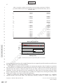
Montos comprometidos en contrato:
Fondef
$ 158,00
millones
Instituciones
$ 122,85
millones
Empresas
$ 228,50
millones
Otros
B.-
EJECUCIÓN
1.
Fecha toma de razón:
06/12/2004
2.
Plazo contractual en meses:
28 meses
3.
Fecha efectiva de inicio:
06/12/2004
4.
Fecha de término efectiva):
30/07/2007
5.
Duración efectiva:
31 meses
$
millones
6.
El proyecto tuvo una duración total de 31 meses. El financiamiento por FONDEF se efectuó durante 28
meses.
Montos efectivamente aportados:
•
Fondef
$ 155,303 millones
Instituciones
Empresas
Otros
$ 122,873 millones
$ 229,913 millones
$
0 millones
Costo Total del Proyecto
El costo total del proyecto fue de 509.35 millones de pesos.
•
Aportes de Fondef.
El monto total rendido y aprobado por FONDEF es de $ 153.632.730 ciento cincuenta y tres
millones seiscientos treinta y dos mil setecientos treinta pesos. La diferencia de $ 1.670.564 un millón
seiscientos setenta mil quinientos sesenta y cuatro pesos con respecto a lo girado por FONDEF ha sido
reintegrada mediante cheque nominativo cruzado a nombre de CONICYT por el mismo monto.
Las instituciones beneficiaras declaran haber utilizado el subsidio para financiar los recursos
que consulta el proyecto.
•
Aporte de los beneficiarios.
La institución hizo aportes a la ejecución del proyecto con recursos valorados en $ 352,786 millones
de pesos. Dicho monto lo enteraron con $ 122,873 millones de pesos en recursos de las propias instituciones
beneficiarias y con $ 229,913 millones de pesos en recursos aportados por las empresas y otras contrapartes
del proyecto.
Los recursos declarados de contraparte, satisfacen el porcentaje mínimo exigible por bases del
concurso.
Las instituciones beneficiarias declaran que los montos detallados de los aportes de las
diferentes fuentes se encuentran en el ANEXO 3 de este informe.
7.
Objetivos y Resultados obtenidos
Objetivos Generales
El objetivo principal del proyecto es desarrollar herramientas, aplicaciones y servicios
computacionales, que aprovechen en forma efectiva las tecnologías asociadas a internet para
modernizar el sistema financiero nacional apoyando una mejor gestión de carteras de inversión en
activos transados en el mercado nacional e internacional.
Los desarrollos se focalizarán preferentemente en la problemática de los fondos de pensiones,
pero sus resultados impactarán la gestión de otras carteras de inversión como las administradas
por compañías de seguros y fondos mutuos, entre otros.
Esta modernización se apoyará tanto en el estado del arte metodológico mundial como en
investigación científica que aborde la problemática de mercados financieros poco profundos como
el nacional, con activos que se transan con una baja frecuencia (thin markets), lo que dificulta el
uso de numerosos procedimientos y metodologías utilizadas en los mercados desarrollados.
De este modo se pretende (1) apoyar una gestión más eficiente de las carteras al incluirse mayor
información relativa a retornos y riesgos involucrados, (2) hacer un análisis de estrategias de
inversión que apoye la asignación de activos (asset allocation), (3) apoyar funciones de medición y
gestión del riesgo y (4) establecer un conjunto de benchmarks para diversas carteras de inversión.
Todo lo anterior busca favorecer la gestión e información para directivos y usuarios y, en ultimo
término, la competitividad y desempeño de la industria.
Objetivos Específicos
1) Generar conocimiento científico
2) Realizar desarrollos tecnológicos
3) Generar información
4) Desarrollar mecanismos de transferencia
5) Formar investigadores y profesionales especializados
8.
Objetivos y Resultados No obtenidos
No hay
9.
Apreciación de impacto del proyecto.
Las instituciones declaran que de acuerdo a su evaluación de impacto, el proyecto ha generado
y está en proceso de generar los siguientes impactos.
•
Científico-Tecnológico
•
Obtenido: Nuevas metodologías de valorización y gestión del riesgo principalmente para
mercados con pocas transacciones como son los mercados de economías emergentes como
la chilena. Esto se ha traducido en publicaciones, tesis de magíster y presentaciones en
conferencias académicas internacionales.
•
En proceso de obtención: Nuevas publicaciones en preparación orientadas a formas de
gestionar carteras de inversión y a modelos multi-activos.
•
•
•
9.
Económico-Social
•
Obtenido: Mejor valorización de carteras de inversión para todos los Fondos Mutuos del
País y para algunas otras instituciones financieras del país, lo que transparenta los mercados
y permite una mejor competencia y asignación de recursos financieros.
•
En proceso de obtención: Mejores decisiones de inversión y de gestión del riesgo para
carteras de inversión de las instituciones financieras del país a medida que vayan adoptando
las herramientas que actualmente están en fase de prueba.
Institucional
•
Obtenido: -Fortalecimiento del FINlabUC-Laboratorio de Investigación Avanzada
en Finanzas tanto en actividad, reconocimiento y equipamiento.
-Fortalecimiento del programa de Magíster en Ciencias de la Ingeniería
con incremento en el número de alumnos que se especializan en finanzas a
nivel de postgrado
-Fortalecimiento de Relaciones con Sector Productivo
-Fortalecimiento de las relaciones de Cooperación Internacional
•
En proceso de obtención: -Incremento en los fortalecimientos institucionales anteriores.
Ambiental
•
Obtenido: No existen
•
En proceso de obtención: No existen
Plan de trabajo.
El Plan de trabajo se estructuró en torno al desarrollo de 5 subtemas que se denominaron:
PortfolioValue, PortfolioBenchmarks, PortfolioRisk, RiskMatrix, AssetAllocation, todos los cuales
en conjunto reciben la denominación RiskPortfolio.
Estos subtemas se estructuraron como subproyectos de I&D dando origen a Tesis de Magíster y
Memorias de Título, Presentaciones a Congresos, Publicaciones, Módulos computacionales y
finalmente 3 servicios: SVC, Indices, y Portfolio.
Las instituciones declaran que el plan de trabajo que representa las actividades del proyecto
se encuentra en el ANEXO 2 de este informe.
10.
Infraestructura y bienes adquiridos por el proyecto
Las instituciones beneficiarias declaran tener inventariados todos los bienes adquiridos por el
proyecto y declarados en ANEXO 4 de este Informe, los que están a cargo de personal de la
institución y se encuentran asignados a las unidades institucionales que se indican en ese
Anexo.
II PARTE. INFORME EJECUTIVO
Código Proyecto: D03I1039
Nombre del Proyecto: DESARROLLO DE HERRAMIENTAS COMPUTACIONALES
PARA OPTIMIZAR LA GESTION DE CARTERAS DE INVERSION EN MERCADOS EMERGENTES:
APLICACION A LOS FONDOS DE PENSIONES EN CHILE
La información entregada en esta parte del documento debe ser sólo la
que puede ser de dominio público.
COMISION NACIONAL DE INVESTIGACION CIENTIFICA Y TECNOLOGICA
FOMENTO AL
DESARROLLO
CIENTIFICO Y
TECNOLOGICO
BERNARDA MORIN 495 • CASILLA 297-V• CORREO 21• FONO: 3654400 • FAX: 6551394 • CHILE
1
RESUMEN EJECUTIVO
Describa en no más de una página la problemática u oportunidades que llevó a formular este proyecto
(origen), su desarrollo, los resultados logrados y la proyección del mismo.
El objetivo principal del proyecto es desarrollar herramientas, aplicaciones y servicios
computacionales, que aprovechen en forma efectiva las tecnologías asociadas a Internet para
modernizar el sistema financiero nacional apoyando una mejor gestión de carteras de inversión
en activos transados en el mercado nacional e internacional. Los desarrollos se focalizan
preferentemente en la problemática de los fondos de pensiones, pero sus resultados impactan
la gestión de otras carteras de inversión como las administradas por compañías de seguros y
fondos mutuos. Esta modernización se apoya tanto en el estado del arte metodológico mundial
como en investigación científica que aborde la problemática de mercados financieros poco
profundos como el nacional, con activos que se transan con una baja frecuencia (thin markets),
lo que dificulta el uso de numerosos procedimientos y metodologías utilizadas en los mercados
desarrollados.
De este modo se pretende (1) apoyar una gestión más eficiente de las carteras al incluirse
mayor información relativa a retornos y riesgos involucrados, (2) hacer un análisis de
estrategias de inversión que apoye la asignación de activos (asset allocation), (3) apoyar
funciones de medición y gestión del riesgo y (4) establecer un conjunto de benchmarks para
diversas carteras de inversión. Todo lo anterior busca favorecer la gestión e información para
directivos y usuarios y, en ultimo término, la competitividad y desempeño de la industria.
El impacto económico y social de este proyecto es extremadamente alto, considerando que
sólo el sistema de AFPs administra más de 100 billones de dólares, por lo que incrementos
marginales en las rentabilidades, que se derivarían de la disponibilidad de mejores
herramientas e información para gestionar los fondos y controlar sus riesgos, crearían una gran
riqueza que sería capturada en su gran mayoría por los afiliados, aumentando el bienestar de
los pensionados. Asimismo, este incremento en el valor de los fondos impulsaría el desarrollo
de la economía nacional, aumentando el ahorro nacional y mejorando la asignación de
recursos. La evaluación social reconoce por una parte que hay una demanda insatisfecha por
tecnologías y servicios de gestión del riesgo y por otra la inexistencia de productos en el
mercado internacional que aborden la problemática específica del mercado nacional.
El proyecto generó múltiples resultados en ámbitos económico-sociales, científico-tecnológicos,
e institucionales de gran impacto.
En primer lugar dio origen a 3 nuevos servicios de gestión del riesgo que se distribuyen por
Internet a través de RiskAmerica: Servicio SVC, (que valoriza diariamente instrumentos de
renta fija con pocas transacciones), Servicio Índices (que entrega benchmarks con el
comportamiento del mercado para diversas clases de activos) y Servicio Portfolio (que entrega
información de retorno, riesgo y performance para carteras del mercado y propias). Estos
servicios ya están siendo utilizados por muchas instituciones financieras del país.
Además el proyecto generó publicaciones en revistas y presentaciones en congresos
internacionales, y apoyó la realización de tesis de magíster y memorias de título, fortaleciendo
las actividades del FINlabUC-Laboratorio de Investigación Avanzada en Finanzas de la
Pontificia Universidad Católica de Chile.
ABSTRACT.
The main objective of this project is to develop tools, software applications and services that
use Internet technologies to provide better portfolio management for domestic and world market
assets and modernize the Chilean financial markets. Although the new developments are
primarily focused on pension funds, results can also be used for other portfolios like mutual
funds or those managed by insurance companies. This market modernization is supported by
standard state-of-the-art methodologies as well as new specific research on thin markets, a
characteristic of Chilean financial markets which imposes difficulties in the use of many
methodologies common in developed markets.
The goals of the project are (1) to induce a more efficient portfolio management which uses
better risk and return information, (2) to analyze investment strategies and support the asset
allocation process, (3) to improve risk management and measurement, (4) to define a set of
portfolio benchmarks; thus, the goal is to help portfolio owners and managers, by providing
better information and management tools, and improving industry competition and performance.
The economic and social impacts of this project are extremely high, considering that the AFPsystem manages over US$ 100 billions. Thus, marginal increases on returns, due to better
tools and information for managing funds and controlling risks, create a huge wealth, most of it
transferred to fund members, increasing their welfare. This return increase would in turn
stimulate the economy, increasing savings and improving resource allocation. The social project
evaluation recognizes that there is an unsatisfied demand for technologies for risk management
and that there are no available products in international markets that satisfy national market
requirements.
The project had multiple results with great impact in economic-social, scientific-technological
and institutional scope.
First it originated three new risk management services distributed by RiskAmerica using
Internet: SVC Service (which prices fixed-income instruments with few market transactions),
Indices Service (which provides benchmarks on market behavior of several asset classes), and
Portfolio Service (which provides risk, return and performance information for market and
private portfolios). These services are already been used by many financial institutions in Chile.
The project also generated journal publications and congress presentations and provided
support for master´s and undergraduate thesis, strengthening the activities of the FINlabUCLaboratorio de Investigación Avanzada en Finanzas de la Pontificia Universidad Católica de
Chile.
2
SINTESIS DE RESULTADOS DEL PROYECTO
RESULTADO
Nuevos productos
Nuevos procesos
Nuevos servicios
Contratos empresas productoras
Patentes
Registro de variedades vegetales
cantidad
RESULTADO
Importancia económica-social
Productos mejorados
Procesos mejorados
Servicios mejorados
3
Convenios (contratos) para proyecto
de escalamiento.
Marcas
Otros registros de propiedad
cantidad
Otro (especificar)
Otro (especificar)
Importancia científica-tecnológica
Capacidades científico-tecnológicas obtenidas:
-Capacidad de desarrollar metodologías e implementar soluciones en el ámbito de la Ingeniería
Financiera y Gestión del Riesgo
Otros Resultados C&T
cantidad
Otros Resultados C&T
Artículos revista nacional, ISSN
Artículos revista nacional
Artículos revista internacional, ISSN
Artículos revista internacional
3
Artículos revista nacional, ISI
Capítulos libro nacional, ISBN
Artículos revista internacional, ISI
Capítulos libro nacional
3
Libros publicación nacional
Capítulos libro internacional, ISBN
Seminarios nacionales*1
Capítulos libro internacional
Seminarios internacionales*2
Libros publicación internacional
1
Congresos nacionales*1
Proyectos I&D
Congresos internacionales*2
Tesis doctorales
Simposios nacionales*1
Tesis magister
Simposios internacionales*2
Postdoctorados
Cursos*
Proyectos de títulos
Reconocimientos de laboratorio
Talleres*
Presentaciones en Congresos Internacionales
Otro (especificar)
9
Importancia ambiental
Propuestas de normativa
Otros (especificar)
Otro (especificar)
*1.realizados por el proyecto, con expositores y/o ponencias nacionales.
*2:realizados por el proyecto, con expositores y/o ponencias de extranjeros.
cantidad
4
3
3
CAPACIDADES CIENTIFICO-TECNOLOGICAS, PRODUCTOS Y
SERVICIOS DESARROLLADOS POR EL PROYECTO. .
Durante la realización del proyecto se desarrolló la capacidad de desarrollar metodologías e
implementar soluciones en el ámbito de la Ingeniería Financiera y Gestión del Riesgo.
Los tres principales servicios ya desarrollados se distribuyen vía Internet como módulos
independientes de la plataforma RiskAmericaPlus. Estos son:
Servicio 1: Módulo SVC
El SVC o Sistema de Valorización de Carteras consiste en un módulo del servicio
RiskAmericaPlus cuyo objetivo es asignarle una TIR a cada nemotécnico solicitado.
El usuario envía vía Web un archivo indicando los nemotécnicos asociados a su cartera,
devolviendo el sistema la TIR que el modelo le asigna a cada uno. La TIR del modelo
depende de si el activo fue transado ese día, de cuál es la curva de referencia para el día (la
que es actualizada diariamente) y de la historia de spreads que este nemotécnico ha
exhibido respecto de la curva en el pasado.
Servicio 2: Módulo Índices
Este módulo entrega información referida al comportamiento del mercado financiero. Esta
descripción se realiza en términos de distintas familias y clases de activos, incluyéndose
tanto renta fija como variable.
Para cada uno de los más de 100 índices existentes se entrega información de su
composición así como de su comportamiento en términos de retornos y riesgos.
Asimismo, se pueden comparar y realizar análisis entre los distintos índices:
Se entrega además la posibilidad de construir y índices personalizados:
También se pueden cargar índices generados externamente
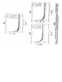
Servicio 3: Módulo Portfolio
Este módulo entrega información de de riesgo, retorno y performance tanto de carteras
existentes del mercado, como de carteras propias.
En Información de Mercado entrega información información de riesgo, de retornos y de
performance de carteras públicas de AFP y de Fondos Mutuos, como se muestra en las
siguientes páginas web:
En Riesgo Absoluto se entregan herramientas para calcular el Value-at-Risk de carteras
propias tanto por métodos paramétricos como por simulación histórica.
En Riesgo Relativo se entregan herramientas para calcular el Tracking Error y el VaR
Relativo a entre dos carteras.
En Asset Allocation se entregan herramientas para calcular carteras con combinaciones
riesgo-retorno óptimas.
En Análisis de Desempeño se entregan herramientas para calcular carteras el performance
de carteras definidas por el usuario.
4
RESULTADO DE EVALUACIÓN EX-POST DESARROLLADA POR
LA INSTITUCIÓN
Tal como se plantea en la Formulación del proyecto, el beneficio social principal de este
proyecto se genera al contribuir a la modernización del mercado financiero nacional. Un
resultado exitoso en cuanto a nuevas herramientas de gestión de carteras, como es el
caso de lo ocurrido con este proyecto debiera inducir que las administradoras de fondos
de pensiones, pueden mejorar la gestión de sus carteras y de esta manera obtener
mayores retornos de sus inversiones, sin incrementar el riesgo asumido.
El principal impacto económico social del proyecto es el Incremento Marginal de la
Rentabilidad aplicado a una Fracción de los Fondos Potenciales que pudieran verse
beneficiados con las herramientas de gestión de carteras desarrolladas. Por último, se
debe estimar el adelantamiento de los flujos (en número de años) que representa la
realización del proyecto comparado con la situación base sin proyecto (i.e. se estima que
si no hubiera habido proyecto, otro similar se hubiera desarrollado teniendo el mismo
impacto después).
Los cuatro parámetros anteriores son difíciles de estimar y de ellos depende el resultado
de los indicadores económicos-sociales.
En la Evaluación ex–ante presentada en la formulación del proyecto se asumieron los
siguientes valores para estos parámetros:
Incremento Marginal de la Rentabilidad = 0,25%
Fracción = 25% de las administradoras* 60% de los activos = 15%
Fondos Potenciales = MMUS$ 40.000
Adelantamiento = 1 año (si no se hace el proyecto los flujos se realizan 1 año después).
Con lo que el beneficio económico-social por año se estimó en US$ 15 millones.
Se puede señalar que desde la formulación del proyecto uno de los parámetros se ha
incrementado significativamente, al aumentar el parámetro Fondos Potenciales subió
al año 2007 a más de MM US$100.000, es decir 2,5 veces mayor que el valor estimado
en la Formulación. Esto permitiría dividir por 2,5 alguno de los indicadores anteriores
(por ejemplo suponer que el Incremento Marginal de la Rentabilidad fuera 0,1 en vez
de los 0,25 asumidos originalmente) y conservar el valor de los indicadores originales.
Debido a lo anterior, una evaluación conservadora mantendría los indicadores
económico-sociales presentados en la Formulación inicial, siendo sus flujos netos:
.
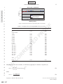
FLUJO NETO
Ingresos
Costos
Inversión
Costo total I+D
Fondef
Beneficio neto
TIR
VAN (10%) MM$
VAN/VAI
VAN/FONDEF
Nota: M/N = moneda nacional
M/E = moneda extranjera
.
0
0
0
290
97
-290
568,06%
9.244
18,90
50,14
0
0
-509
219
97
290
10.754
276
-509
0
0
10.987
238
136
-6
0
0
108
238
136
-6
119
70
-6
119
71
-6
0
38
-6
0
38
-6
0
0
-6
108
55
54
-32
-32
6
III PARTE. INFORME DE GESTIÓN
Código Proyecto: D03I1039
Nombre del Proyecto:
DESARROLLO DE HERRAMIENTAS COMPUTACIONALES PARA OPTIMIZAR
LA GESTION DE CARTERAS DE INVERSION EN MERCADOS EMERGENTES: APLICACION A LOS
FONDOS DE PENSIONES EN CHILE
Instituciones Participantes: Pontificia Universidad Católica de Chile
Otros Participantes:
AFP Habitat S.A.
RiskAmerica- Dictuc S.A.
Director del Proyecto: .Gonzalo Cortazar Sanz, Firma:...........................
Fecha de emisión : 23/07/2007
FOMENTO AL
DESARROLLO
CIENTIFICO Y
TECNOLOGICO
COMISION NACIONAL DE INVESTIGACION CIENTIFICA Y TECNOLOGICA
BERNARDA MORIN 495 • CASILLA 297-V• CORREO 21• FONO: 3654400 • FAX: 6551394 • CHILE
1. OBJETIVOS DEL PROYECTO
1.1 OBJETIVOS GENERALES
Programados
El objetivo principal del proyecto es desarrollar herramientas, aplicaciones y servicios
computacionales, que aprovechen en forma efectiva las tecnologías asociadas a internet para
modernizar el sistema financiero nacional apoyando una mejor gestión de carteras de inversión
en activos transados en el mercado nacional e internacional.
Los desarrollos se focalizarán preferentemente en la problemática de los fondos de pensiones,
pero sus resultados impactarán la gestión de otras carteras de inversión como las
administradas por compañías de seguros y fondos mutuos, entre otros.
Esta modernización se apoyará tanto en el estado del arte metodológico mundial como en
investigación científica que aborde la problemática de mercados financieros poco profundos
como el nacional, con activos que se transan con una baja frecuencia (thin markets), lo que
dificulta el uso de numerosos procedimientos y metodologías utilizadas en los mercados
desarrollados.
De este modo se pretende (1) apoyar una gestión más eficiente de las carteras al incluirse
mayor información relativa a retornos y riesgos involucrados, (2) hacer un análisis de
estrategias de inversión que apoye la asignación de activos (asset allocation), (3) apoyar
funciones de medición y gestión del riesgo y (4) establecer un conjunto de benchmarks para
diversas carteras de inversión. Todo lo anterior busca favorecer la gestión e información para
directivos y usuarios y, en ultimo término, la competitividad y desempeño de la industria.
No obtenidos
Obtenidos no programados
Aún cuando desde un principio se esperaba no restringir el impacto del proyecto sólo a la
industria de las AFP sino también a la de otros actores de la industria financiera, el impacto
sobre la industria de los Fondos Mutuos fue más fuerte y más anticipado de lo programado.
Es así como desde marzo de 2006 los precios para todos los instrumentos de renta fija son
entregados vía Internet a todos los fondos mutuos nacionales como precio oficial para ser
utilizados en el cálculo diario de la cuota de todos los fondos mutuos, según circular de la
Superintendencia de Valores y Seguros y en acuerdo con la Asociación de Administradoras de
Fondos Mutuos de Chile. Asimismo, ya se han iniciado contactos internacionales que pueden
llevar a exportar algunas de las tecnologías desarrolladas.
1.2 OBJETIVOS ESPECIFICOS
Programados
El proyecto en sus diversos ámbitos de acción tiene los siguientes objetivos específicos:
1) Generar conocimiento científico acerca del comportamiento de los mercados
financieros nacionales y su interrelación con los mercados internacionales. Esta
investigación deberá generar información de interés para Chile y para entender el
comportamiento de los mercados en los diversos mercados emergentes.
2) Realizar desarrollos tecnológicos que se expresen en nuevas metodologías y en
herramientas, aplicaciones y servicios computacionales que tengan un impacto
significativo en el manejo de los recursos de los fondos de pensiones nacionales.
Este impacto se producirá a través de: a) la optimización de las carteras de
inversión de las administradoras sujetas a las regulaciones existentes, y b) de
mejoramientos sistémicos (a nivel de la industria) producto del mayor conocimiento
de los riesgos asociados a los diversos activos, lo que debiera permitir ajustar
regulaciones y restricciones de inversión de modo de poder limitar las exposiciones
al riesgo deseadas incurriendo en un menor costo en términos de rentabilidad.
3) Generar información en la forma de indicadores de gestión comparativa que sea
objetiva y confiable y que apoye la modernización, transparencia y desarrollo del
mercado financiero nacional.
4) Desarrollar mecanismos de transferencia efectiva de resultados de modo de
maximizar el impacto sobre el sistema productivo del país y las oportunidades
comerciales del proyecto asegurando su sustentabilidad.
5) Formar investigadores y profesionales especializados en aplicaciones
financieras de alto nivel. Una condición necesaria para sustentar el desarrollo de la
industria de las aplicaciones financieras en Chile, y de colaborar de ese modo a
modernizar el mercado financiero, es contar con el capital humano capacitado que
actúe tanto como oferente y como contraparte de estas aplicaciones.
No obtenidos
-Obtenidos no programados
--
2. RESULTADOS DEL PROYECTO
2.1
PRODUCTOS, SERVICIOS Y/O PROCESOS. Detalle según tabla.
NOMBRE
DESCRIPCIÓN
1
Módulo SVC
2
Módulo Indices
3
Módulo Portfolio
2.2
TIPO DE
RSULTADO
P: PROGRAMDO
I: INESPERADO
Módulo Computacional Vía WEB que Valoriza P
Instrumentos de Renta Fija (PortfolioValue)
Módulo Computacional Vía WEB que Entrega P
Información
de
Referencia
de
Mercado
(PortfolioBenchmarks)
Módulo Computacional Vía WEB que entrega P
herramientas de gestión para Carteras de Inversión
(PortfolioRisk+AssetAllocation+RiskMatrix)
TIPO DE
INNOVACIÓN
*
ESTADO
DEL MEDIDAS DE
PROTECCIÓN***
DESARROLLO**
Nuevo
Servicio
Nuevo
Servicio
Comercializción
No es posible de ser
patentado
Comercializción
No es posible de ser
patentado
Nuevo
Servicio
Comercializción
No es posible de ser
patentado
PAQUETE TECNOLÓGICO
PRODUCTO,
PROCESO
SERVICIO (nombre)
o PAQUETE TECNOLÓGICO
( enumere el conjunto de elementos que compone el paquete tecnológico asociado al producto o proceso desarrollado)
Módulo SVC
Set integrado de herramientas computacionales vía Internet orientadas a la valorización de instrumentos financieros
Módulo Indices
Set integrado de herramientas computacionales vía Internet orientadas a generar y entregar información relativa al
comportamiento de los mercados financieros
Módulo Portfolio
Set integrado de herramientas computacionales vía Internet orientadas a apoyar la gestión de carteras de inversión.
2.3
COMPETITIVIDAD DE LOS PRODUCTOS, SERVICIOS Y/O PROCESOS MEJORADOS(agregue más columnas si es necesario)
PRODUCTO SERVICIO VENTAJA*(naturaleza
O PROCESO (nombre)
beneficio)
Módulo SVC
Módulo Indices
Módulo Portfolio
del MONTO
MM$)
Calidad de Información
Calidad de Información
Calidad de Herramientas
(valor actual del beneficio en PRODUCTO, SERVICIO O PROCESO CON QUE DESVENTAJAS
COMPITE (nombre, breve descripción)
(exprese cuantitativamente)
Valor mejor información usuario
Valor mejor información usuario
Valor mejor información usuario
Sistemas Internos/otros proveedores
Sistemas Internos/ otros proveedores
Sistemas Internos/
Dependencia externa
Dependencia externa
Dependencia externa
2.4
MERCADO
PRODUCTO SERVICIO
O PROCESO (nombre)
Módulo SVC
Módulo Indices
Módulo Portfolio
OFERTA ACTUAL
Volumen
Indique unidades
240 Usuario-Mes
36 Usuario-Mes
18 Usuario-Mes
DEMANDA ESTIMADA
MM$ (2007)
180
10
8
Volumen
Indique unidades
MM$ (2007)
720 Usuario-Mes 240
720 Usuario-Mes 120
720 Usuario-Mes 210
%DE
PARTICIPACIÓN
ESPERADA
MERCADO
60%
60%
60%
AÑOS *
CANALES DE
COMERCIALIZACIÓN
4
4
4
RiskAmerica
RiskAmerica
RiskAmerica
DE
2.5
VALORIZACIÓN ECONÓMICA DE LOS RESULTADOS DEL PROYECTO
incorpórelos en el plan de negocios)
Indique en forma sintética. Los detalles y justificación
PRODUCTO, SERVICIO O VALOR
(MM%)
PROCESO
MODALIDAD DE LA TRANSFERENCIA
ACTUAL CRITERIOS PARA LA FIJACIÓN DE PRECIO
SVC + Índices+ Portfolio MM$781
2.6
No existen consideraciones especiales
Excedentes de Dictuc SA que es de propiedad de la PUC
TRANSFERENCIA TECNOLÓGICA
PRODUCTO
PROCESO
SERVICIO
O INSTITUCIÓN /EMPRESA PRODUCTORA )
SVC + Índices+ Portfolio RiskAmerica
PARTICIPÓ EN EL CONTRATO DE TRANSFERENCIA, VENTA O LICENCIA.
DESARROLLO
DEL
PROYECTO
Si
MM$ 300
Continuación
COSTO (estimado en MM$ de 1999 de las FUENTES DE FINANCIAMIENTO
PRODUCTO
ACCIONES FUTURAS
SERVICIO
O (diga cuáles son las acciones, recursos y plazos, no desarrolladas, ni proveídos por el acciones necesarias faltantes para la
PROCESO (nombre) proyecto que permitirán la explotación de los resultados del proyecto)
transferencia)
SVC
+
Índices +
Portfolio
2.7
Contactos individuales y eventos de promoción
VENTAS INSTITUCIONALES (de productos y servicios del proyecto, no consideradas en el pto. 2.6)
CONCEPTO (qué se vendió)
AÑO (que se efectúo la venta)
MONTO (en MM$ del año 1999)
2.8
CAPACIDADES TECNOLOGICAS. Detalle las capacidades tecnológicas creadas o mejoradas con este proyecto. (Ejemplos en APENDICE·1 )
CAPACIDADES TECNOLÓGICAS
PRODUCTOS O SERVICIOS QUE SE
USUARIOS DE LOS PRODUCTOS
PUEDEN OBTENER DE LAS CAPACIDADES
SERVICIOS
.
Nº
Nombre
Nombre del producto o servicio
Nombre del usuario
1 Capacidad de desarrollar metodologías e Nuevos Servicios y Capacitación en gestión del riesgo
Instituciones financieras y regulatorias
implementar soluciones en el ámbito de la
Ingeniería Financiera y Gestión del Riesgo
O
2.9
CAPACIDAD INSTITUCIONAL PARA GESTIÓN CIENTÍFICO- TECNOLÓGICA (describa las principales capacidades creadas o fortalecidas
por el proyecto, señalando expresamente cual es el caso)
Fortalecimiento del FinlabUC-Laboratorio de Investigación Avanzada en Finanzas lo que permite abordar nuevos proyectos de investigación aplicada con
nuevos desarrollos tecnológicos asociados.
2.10
FORMACIÓN DE PERSONAL
FORMACION CIENTIFICO-TECNOLOGICA DE PARTICIPANTES EN EL PROYECTO.
Nº
1
Tipo
1= Proyectos de títulos
2= Tesis de magister
3= Tesis doctorales
4= Posdoctorados
2
2
2
3
2
Título de Curso o taller o del
proyecto de título o de la tesis
"Modelo estocástico
multicommodity para la
dinámica de precios de
contratos futuros. Selección
y estimación del modelo
utilizando componentes
principales comunes y filtro
de Kalman"
“Estimación de Spreads por
Liquidez en un Mercado
con Pocas Transacciones:
El Caso del Mercado de
Bonos del Banco Central de
Chile”
“Metodología e
Implementación de
Métodos de VALUE AT
RISK en Mercados de
Renta Fija con baja
Frecuencia de
Nombre del
participante
RUT
Disciplina
(disciplina
Fondecyt
predominante)
Institución o empresa
(en que realizó la
actividad de formación;
indíquelos todos)
Mes y Año
(en que el
participante logró
la formación)
Ciudad/País
(donde se realizó
la formación;
indíquelos todos)
FELIPE
SEVERINO
DIAZ
14146082-K
Finanzas
Pontificia Universidad
Católica de Chile
Marzo, 2007
Santiago-Chile
PEDRO
MATÍAS
MORAL MESA
13551671-6
Finanzas
Pontificia Universidad
Católica de Chile
Enero, 2006
Santiago-Chile
Finanzas
Pontificia Universidad
Católica de Chile
Diciembre, 2005
Santiago-Chile
ALEJANDRO
ADRIAN
BERNALES
SILVA
Nº
Tipo
1= Proyectos de títulos
2= Tesis de magister
3= Tesis doctorales
4= Posdoctorados
4
2
5
1
6
1
7
1
Título de Curso o taller o del
proyecto de título o de la tesis
Transacciones”
“Modelos Estocásticos de
Precios de Commodities y
Estimación Conjunta de la
Dinámica de dos
Commodities Mediante el
Filtro de Kalman”
“Bonos Corporativos: una
Revisión del Mercado y una
Aproximación a un Método
Práctico de Valorización”
“Valorización de
Instrumentos Financieros en
Mercados con Pocas
Transacciones: Análisis de
una Metodología Basada en
un Modelo Dinámico para
la Tasa Cero Real en Chile”
“Decisiones de Asset
Allocation en Carteras de
Inversión de las AFP:
Aplicación del Modelo de
Black & Litterman”
Nombre del
participante
CARLOS
IGNACIO
MILLA
GONZALEZ
RUT
13922911-8
CLAUDIO
EDUARDO
HELFMANN
SOTO
JOSE LUIS
MANIEU
ESPINOSA
RODRIGO
ALFONSO
IBANEZ
VILLARROEL
13548272-2
Disciplina
(disciplina
Fondecyt
predominante)
Institución o empresa
(en que realizó la
actividad de formación;
indíquelos todos)
Mes y Año
(en que el
participante logró
la formación)
Ciudad/País
(donde se realizó
la formación;
indíquelos todos)
Finanzas
Pontificia Universidad
Católica de Chile
Diciembre, 2005
Santiago-Chile
Finanzas
Pontificia Universidad
Católica de Chile
Diciembre, 2005
Santiago-Chile
Finanzas
Pontificia Universidad
Católica de Chile
Agosto, 2005
Santiago-Chile
Finanzas
Pontificia Universidad
Católica de Chile
Julio, 2005
Santiago-Chile
2.11
DIFUSIÓN Y PUBLICACIONES DE RESULTADOS
PUBLICACIONES RELACIONADAS CON CONTENIDOS DEL PROYECTO.
Nº
1
Tipo
1= libro, 2= cap. de libro
3= art. revista, 4= manuales
técnicos, Otros {especificar}
3
2
3
3
Nombre Publicación
(del cap. libro, del art. revista,
del manual técnico, de otros)
Nombre
(del libro o revista, cuando en la columna anterior
sea un cap. o un art.)
"Term Structure Estimation in
Markets with Infrequent Trading“
Computers & Operations Research
“The Valuation of
International Journal of Finance and
Multidimensional American Real
Economics
Options using the LSM Simulation
Method”
“An N-Factor Gaussian Model of
The Journal of Futures Markets
Oil Futures Prices”
3
Nombre autor(es)
(1)
RUT
Cortazar, G.,
Gravet, M.,
Urzua, J
Cortazar, G,
Schwartz, E. S.
Naranjo, L
60663351-1
9908534-9
13307237-3
60663351-1
Cortazar, G.
Naranjo, L.
60663351-1
12931431-1
12931431-1
IDENTIFICACION (CONTINUACION)
Nº
(1)
Mes y Año
de Edición o
Publicación
Ciudad y País
(donde se editó o
publicó)
1
01/2008
OXFORD,
ENGLAND
2
2007 (por aparecer)
3
03/2006
CHICHESTER,
ENGLAND, W
SUSSEX, PO19
8SQ
HOBOKEN,
USA, NJ, 07030
Páginas
(para cap. de libro o
art. de revista,
de.... a....)
113 – 129
243-268
Editorial
Código
ISBN, ISSN, ISI
(2)
Disciplina
(disciplina Fondecyt
predominante)
PERGAMONELSEVIER
SCIENCE
LTD,
JOHN WILEY
& SONS INC
ISSN: 0305-0548
Computación
Clasificación
1=Científica
2=Tecnológica
3=Difusión
Otras {especificar}
1
ISSN: 1076-9307
Finanzas
1
JOHN WILEY
& SONS INC,
ISSN:0270-7314
Finanzas
1
2.12
PROTECCIÓN DE RESULTADOS
a) PATENTES
Nº
Título
Disciplina
(disciplina
Fondecyt
predominante)
País
(país donde
se solicitó la
patente)
Páginas
(cantidad de
páginas de la
patente )
Observaciones
Estado
(1) Solicitada
(2) Otorgada
Fecha
Otorgamiento
Tipo de patente
(Nacional / Internacional)
Indique país(es) donde rige
1
AUTORES (CONTINUACION PATENTES)
Nº patente
cuadro
anterior
Rut (para nacionales y
extranjeros residentes en
Chile)
Apellido Paterno
Apellido Materno
Nombres
Dueño de la patente
b) OTRAS FORMAS DE PROTECCIÓN
Resultado
Resultados del proyecto
Tipo de protección
El valor comercial de los resultados del proyecto se basan fuertemente en la reputación de
objetividad, rigurosidad y compromiso de permanente innovación que puedan comunicar los
proveedores de los mismos. Es por esto que más que proteger desarrollos la estrategia de
protección consiste en comunicar en forma creíble estos atributos y en ofrecer innovaciones
permanentes difíciles de replicar por otros proveedores.
Establecida (si o no)
Si
2.13
EVENTOS RELACIONADOS CON EL PROYECTO EN QUE PARTICIPO PERSONAL DEL PROYECTO.
A) IDENTIFICACION DE EVENTOS.
Nº
Título o nombre del evento
1 Seminario Internacional de Innovación
Financiera/Lanzamiento RiskAmercaPLUS
2 4th Annual Conference of Asia Pacific
Association of Derivatives
3 Latin American Meeting of the Econometric
Society
4 2006 FMA Annual Meeting
5 2006 Far Eastern Meeting of the Econometric
Society
6 INFORMS Hong Kong International 2006
7 15th annual meeting of the European Financial
Management Association
8 2005 FMA Annual Meeting
9 9th Annual International Conference Real
Options: Theory Meets Practice
10 EFA 2004 Meeting
Tipo de Evento
1=Congreso,
2=Seminario,
3=Taller,
4= Curso,
5=Simposio,
6=Mesa Redonda,
Otro {especificar}
País
(país
donde se
realizó el
evento)
Ciudad
(ciudad dónde
se realizó el
evento)
2
Chile
Santiago
29-03-2007 29-03-2007
2-3
UC-Fondef
1
India
Gurgaon
20-06-2007 22-06-2007
1
APAD-MDI
1
02-11-2006 04-11-2006
1
LAMES-ITAM
11-10-2006 14-10-2006
1
FMA
1
México Ciudad de
México
EEUU Salt Lake
City
China Beijing
9-07-2006
12-07-2006
1
1
1
China Hong Kong 25-06-2006 28-06-2006
España Madrid
28-06-2006 01-07-2006
1
1
Econometric SocietyTsinghua University
INFORMS
EFMA
1
1
EEUU Chicago
Francia Paris
12-10-2005 15-10-2005
23-06-2005 25-06-2005
1
1
FMA
ROG - EDC
1
Holand Maastricht
a
18-06-2004 21-08-2004
1
EFA
1
Fecha de
inicio del
evento
Fecha término
del evento
Clasificación
1=C&T,
2=de Negocios,
3=de Difusión,
4= de
Capacitación,
Otros
{especificar}
Evento organizado por
1= el proyecto
Otros {especificar}
B) IDENTIFICACION DEL PERSONAL DEL PROYECTO QUE PARTICIPO EN EVENTOS
Nº del evento
(Nº de la tabla
anterior)
(1)
6066335-1
Cortazar
Sanz
Gonzalo
Rol en el evento
1= Expositor
2=Asistente
Otro {especificar}
1
4940618-5
Majluf
Schwartz
Sapag
G.
Nicolás
Eduardo
1
1
2
6066335-1
Cortazar
Sanz
Gonzalo
1
3
6066335-1
Cortazar
Sanz
Gonzalo
1
4
6066335-1
Cortazar
Sanz
Gonzalo
1
5
6066335-1
Cortazar
Sanz
Gonzalo
1
6
6066335-1
Cortazar
Sanz
Gonzalo
1
7
6066335-1
Cortazar
Sanz
Gonzalo
1
8
6066335-1
Cortazar
Sanz
Gonzalo
1
9
6066335-1
Cortazar
Sanz
Gonzalo
1
10
6066335-1
Cortazar
Sanz
Gonzalo
1
1
Descripción de la persona vinculada al evento
RUT
Apellido
Apellido
Nombres
paterno
materno
(1) Copie el Nº correspondiente de la tabla anterior
Título de la Exposición
(si fue expositor)
Lanzamiento Oficial de
RiskAmercaPlus
Comentarios Finales
Hedge Funds: Riesgos y
Oportunidades
“A Multicommodity Model of
Futures Prices: Using Futures
Prices of One Commodity to
Estimate the Stochastic Process
of Another”
"Term Structure Estimation in
Markets with Infrequent
Trading"
"Term Structure Estimation in
Markets with Infrequent
Trading"
"Term Structure Estimation in
Markets with Infrequent
Trading"
“Using futures prices of one
commodity to estimate the
stochastic process of another”
"Term Structure Estimation in
Markets with Infrequent
Trading"
“An N-Factor Gaussian Model
of Oil Futures Prices”
“The Valuation of
Multidimensional American
Real Options using the LSM
Simulation Method”
"Term Structure Estimation in
Low-Frequency Transaction
Markets: A Kalman Filter
Approach with Incomplete
Panel-Data"
Certificación
(Si fue asistente)
1= De asistencia
2= De aprobación
Duración
(si fue asistente)
Nº Horas
2.14
Nº RUT
1
COOPERACIÓN INTERNACIONAL Y NACIONAL. COLABORACION DE EXPERTOS
Apellido
Paterno
Schwartz
Apellido
Materno
Greenwald
Nombres
Eduardo
Saul
Institución
de Origen
UCLA
País de
Origen
EEUU
Lugar de
Trabajo en
Chile
En Chile y
Via Web
Fecha
de
Inicio
2004
Fecha
de
término
2007
Tema
Disciplina
Fondecyt
predominan
te
Supervisi Finanzas
ón
Research
Código de
actividades del
proyecto
(en las que
participó)
Research
3
IMPACTOS ACTUALES Y ESPERADOS DE MEDIANO Y LARGO PLAZO
3.1 IMPACTOS ECONOMICO-SOCIALES.
PRODUCIDOS
Mejor valorización de carteras de inversión para todos los Fondos Mutuos del País y para algunas otras
instituciones financieras del país, lo que transparenta los mercados y permite una mejor competencia y asignación
de recursos financieros.
Desde marzo de 2006 los precios para todos los instrumentos de renta fija son entregados vía Internet a todos los
fondos mutuos nacionales como precio oficial para ser utilizados en el cálculo diario de la cuota de todos los fondos
mutuos, según circular de la Superintendencia de Valores y Seguros y en acuerdo con la Asociación de
Administradoras de Fondos Mutuos de Chile.
ESPERADOS
Mejores decisiones de inversión y de gestión del riesgo para carteras de inversión de las instituciones financieras
del país a medida que vayan adoptando las herramientas que actualmente están en fase de prueba.
3..2 IMPACTOS CIENTIFICO-TECNOLOGICOS.
PRODUCIDOS
Nuevas metodologías de valorización y gestión del riesgo principalmente para mercados con pocas transacciones
como son los mercados de economías emergentes como la chilena. Esto se ha traducido en publicaciones, tesis de
magíster y presentaciones en conferencias académicas internacionales.
ESPERADOS
Nuevas publicaciones en preparación orientadas a formas de gestionar carteras de inversión y a modelos multiactivos
3..3 IMPACTOS INSTITUCIONALES.
PRODUCIDOS
-Fortalecimiento del FINlabUC-Laboratorio de Investigación Avanzada en Finanzas tanto en actividad,
reconocimiento y equipamiento.
-Fortalecimiento del programa de Magíster en Ciencias de la Ingeniería con incremento en el número de alumnos
que se especializan en finanzas a nivel de postgrado
-Fortalecimiento de Relaciones con Sector Productivo
-Fortalecimiento de las relaciones de Cooperación Internacional
ESPERADOS
-Incremento en los fortalecimientos institucionales anteriores.
3..4 IMPACTOS AMBIENTALES.
PRODUCIDOS
No existen
ESPERADOS
No existen
3.5 IMPACTOS REGIONALES.
PRODUCIDOS
No existen
ESPERADOS
No existen
4 PLAN DE NEGOCIOS.
A continuación se describen los principales aspectos del Plan de Negocios en ejecución:
4.1 Productos
Se considera la comercialización de 3 módulos de Servicios :
Módulo SVC
Módulo Indices
Módulo Portfolio
4.2 Clientes
Los clientes de los servicios ofrecidos son instituciones financieras (AFP, Bancos, Fodnos Mutuos, Corredoras,
Cias de Seguros, etc), y organismos reguladores (Banco Central, Superintendencias, etc).
4.3 Factores de Éxito
El principal Factor de Éxito es la capacidad de generar y comunicar una reputación de objetividad, rigurosidad
y compromiso de permanente innovación para los Servicios ofrecidos. Para ello se hace necesario mantener activo
un equipo de investigadores haciendo investigación reconocida internacionalmente.
4.4 Comercialización
La comercialización nacional se realizara a través de la plataforma RiskAmerica, la que comunicó al mercado
la incorporación de estos servicios expandidos como RiskAmericaPlus. Se están explorando oportunidades de
internacionalización de los servicios.
4.5 Ventas Actuales y Proyección de Resultados Futuros
Las ventas esperadas de los 3 módulos de Servicios para el año 2007 alcanzan MM$198 las que debieran
incrementarse en los años futuros hasta alcanzar un monto esperado de MM$570 el año 2010.
5. GESTION DEL PROYECTO.
5.1 PLAN DE TRABAJO EFECTIVAMENTE REALIZADO vs. PLAN DE TRABAJO INICIAL.
Comentario:
El proyecto se encuadró bastante bien en el Plan de Trabajo inicial propuesto. Los principales cambios fueron la
extensión de la fecha final del proyecto en 1 mes y que algunos de los resultados programados sufrieron un
reordenamiento en el tiempo.
La razón principal de estos cambios fueron de acuerdo con cambios en la percepción de los requerimientos de los
potenciales clientes.
Enseñanzas obtenidas ¿Qué consideraría para mejorar la formulación y ejecución de un próximo plan?
5.2 GASTO EJECUTADO vs. PRESUPUESTO INICIAL.
Comentario
El proyecto se ajustó bastante bien al presupuesto inicial total presentado, con pequeños ajustes en algunos ítems.
Enseñanza obtenida ¿Qué consideraría para la formulación y ejecución de un próximo presupuesto?
5.3 INSTITUCIONES PARTICIPANTES
A.- AL INICIO DEL PROYECTO
INSTITUCION
APORTES
(comprometido en contrato CONCYT,
pesos de 1996)
ROL
A.F.P. Habitat
Riskamerica/Dictuc SA
P.U.C.
103,500
125,000
122,850
B.-DURANTE EL PROYECTO
INSTITUCION
ROL
A.F.P. Habitat
Riskamerica/Dictuc SA
P.U.C.
APORTES
(reales OBSERVACIONES
(causas o motivo del
efectuados en moneda retiro, incorporación o modificación del aporte)
del año)
104,912
125,001
122,873
C.- ENSEÑANZA OBTENIDA
5.4 RENDICION FINAL DE GASTOS.
INSTITUCIÓN BENEFICIARIA
MONTO
TOTAL MONTO
TOTAL MONTO
MONTO TOTAL
(adjudicado GIRADO
RENDIDO (aprobado) CONTRATO
POR DEVOLUCIÓN
mas reajustes) (2)
(1)
FONDEF (3)
GIRO (3)-(1) *
Pont. Universidad Católica 153.632.760
de Chile
158.000.000
155.303.294
- 1.670.534
O
5.5
ORGANIZACIÓN Y EQUIPO DE TRABAJO
El proyecto se organizó considerando:
Una dirección General: Gonzalo Cortazar
Una unidad de Investigación: Eduardo Schwartz y Gonzalo Cortazar (con apoyo de Jaime Casassus)
Una unidad de Productos y Transferencia a Usuarios: Nicolás Majluf y C Mery (AFP Habitat).
Un pool de profesionales e investigadores que eran asignados a distintos proyecto de acuerdo a las necesidades
Las tareas se gestionaron considerando:
Subproyectos a cargo de distintos profesionales, con reportes semanales internos, reportes mensuales con reunión
directiva ampliada (con participación de prof AFP) y reuniones trimestrales del directorio del proyecto que incluía al
Gte de Inversiones de la AFP.
Enseñanza obtenida:
5.6 OBSERVACIONES, CONCLUSIONES Y RECOMENDACIONES
PROYECTO
1.-Sobre el proyecto
DE LA DIRECCIÓN DEL
2.- Sobre su Institución
3.- Sobre otras instituciones y empresas patrocinantes
4.- Sobre el FONDEF
5.7 OBSERVACIONES, CONCLUSIONES Y RECOMENDACIONES INSTITUCIONALES
IV PARTE. INFORME CIENTÍFICO TECNOLÓGICO
Y ECONÓMICO SOCIAL
Código Proyecto: D03I1039
Nombre del Proyecto:
DESARROLLO DE HERRAMIENTAS COMPUTACIONALES PARA OPTIMIZAR
LA GESTION DE CARTERAS DE INVERSION EN MERCADOS EMERGENTES: APLICACION A LOS
FONDOS DE PENSIONES EN CHILE
Instituciones Participantes: Pontificia Universidad Católica de Chile
Otros Participantes:
AFP Habitat S.A.
RiskAmerica- Dictuc S.A.
Director del Proyecto: .Gonzalo Cortazar Sanz, Firma:...........................
Fecha de emisión : 23/07/2007
FOMENTO AL
DESARROLLO
CIENTIFICO Y
TECNOLOGICO
COMISION NACIONAL DE INVESTIGACION CIENTIFICA Y TECNOLOGICA
BERNARDA MORIN 495 • CASILLA 297-V• CORREO 21• FONO: 3654400 • FAX: 6551394 • CHILE
IV PARTE. INFORME CIENTÍFICO TECNOLÓGICO
Y ECONÓMICO SOCIAL
1.
INDICE
1.1 Índice por Tema de Investigación
1: Modelación y Calibración de Procesos Estocásticos para Precios de Instrumentos en Mercados
con Paneles de Datos Incompletos.
2: Metodologías de Valorización de Derivados escritos sobre Subyacentes con procesos
Completos
3: Metodologías de Medición de Spreads.
4: Metodologías de Medición de Riesgos y de Asignación de Activos (Asset Allocation) para
Carteras de Inversión
5: Modelación y Calibración Conjunta de Procesos Estocásticos de Múltiples Activos.
1.2 Índice por Documento de Resultados
1.2.1 Publicaciones
Cortazar, G., Gravet, M., Urzua, J. (2008) “The Valuation of Multidimensional American Real Options using the
LSM Simulation Method” Computers & Operations Research Vol 35 (2008) 113 – 129
Cortazar, G, Schwartz, E. S., Naranjo, L, (2007) "Term Structure Estimation in Markets with Infrequent Trading“
International Journal of Finance and Economics (por aparecer)
Cortazar, G., Naranjo, L. (2006) “An N-Factor Gaussian Model of Oil Futures Prices” The Journal of Futures
Markets, Vol.26, No. 3, March, 2006, 243-268
1.2.2 Documentos de Trabajo aún no publicados
Cortazar, G, Milla, C. Severino, F. (2007) “A Multicommodity Model of Futures Prices: Using Futures Prices of One
Commodity to Estimate the Stochastic Process of Another”
Cortazar, G, Bernales, A. Beuermann, D. (2007) “Methodology and Implementation of Value-at-Risk Measures
in Emerging Fixed-Income Markets with Infrequent Trading
1.2.3 Tesis de Magíster Finalizadas
"Modelo estocástico multicommodity para la dinámica de precios de contratos futuros. Selección y estimación del
modelo utilizando componentes principales comunes y filtro de Kalman", FELIPE SEVERINO DIAZ, Tesis de
Magíster en Ciencias de la Ingeniería, Pontificia Universidad Católica de Chile, 26-03-2007
“Estimación de Spreads por Liquidez en un Mercado con Pocas Transacciones: El Caso del Mercado de Bonos del
Banco Central de Chile”, PEDRO MATÍAS MORAL MESA, Tesis de Magíster en Ciencias de la Ingeniería,
Pontificia Universidad Católica de Chile, 17-01-2006
“Metodología e Implementación de Métodos de VALUE AT RISK en Mercados de Renta Fija con baja Frecuencia
de Transacciones” ALEJANDRO ADRIAN BERNALES SILVA, Tesis de Magíster en Ciencias de la Ingeniería,
Pontificia Universidad Católica de Chile, 23-12-2005
“Modelos Estocásticos de Precios de Commodities y Estimación Conjunta de la Dinámica de dos Commodities
Mediante el Filtro de Kalman” CARLOS IGNACIO MILLA GONZALEZ, Tesis de Magíster en Ciencias de la
Ingeniería, Pontificia Universidad Católica de Chile, 23-12-2005
1.2.4 Memorias de Título Finalizadas
“Bonos Corporativos: una Revisión del Mercado y una Aproximación a un Método Práctico de Valorización” ,
Memoria Escuela de Ingeniería, Pontificia Universidad Católica de Chile, CLAUDIO EDUARDO HELFMANN
SOTO , 31-12-2005
“Valorización de Instrumentos Financieros en Mercados con Pocas Transacciones: Análisis de una Metodología
Basada en un Modelo Dinámico para la Tasa Cero Real en Chile” JOSE LUIS MANIEU ESPINOSA, Memoria
Escuela de Ingeniería, Pontificia Universidad Católica de Chile 12-08-2005
“Decisiones de Asset Allocation en Carteras de Inversión de las AFP: Aplicación del Modelo de Black &
Litterman”, RODRIGO ALFONSO IBANEZ VILLARROEL, Memoria Escuela de Ingeniería, Pontificia
Universidad Católica de Chile, 26-07-2005
1.2.5 Presentaciones en Congresos Académicos
Cortazar, G, Milla, C. Severino, F. (2007) “A Multicommodity Model of Futures Prices: Using Futures Prices of One
Commodity to Estimate the Stochastic Process of Another”,4th Annual Conference of Asia Pacific Association of
Derivatives (APAD), Gurgaon, India, June 20-22, 2007
Cortazar, G, Schwartz, E. S., Naranjo, L, (2006) "Term Structure Estimation in Markets with Infrequent Trading".
Latin American Meeting of the Econometric Society (LAMES) , ITAM, Ciudad de México, Nov. 2-4, 2006
Cortazar, G, Schwartz, E. S., Naranjo, L, (2006) "Term Structure Estimation in Markets with Infrequent Trading".
2006 FMA Annual Meeting , Salt Lake City, Oct. 11 - 14, 2006
Cortazar, G, Schwartz, E. S., Naranjo, L, (2006) "Term Structure Estimation in Markets with Infrequent Trading".
2006 Far Eastern Meeting of the Econometric Society, Beijing, July 9-12, 2006
Cortazar, G, Milla, C. Severino, F. (2006) “Using futures prices of one commodity to estimate the stochastic process
of another” INFORMS Hong Kong International 2006, Hong Kong, June 25-28, 2006
Cortazar, G, Schwartz, E. S., Naranjo, L, (2006) "Term Structure Estimation in Markets with Infrequent Trading".
15th annual meeting of the European Financial Management Association, Madrid, June 28-July 1, 2006
Cortazar, G., Naranjo, L. (2005) “An N-Factor Gaussian Model of Oil Futures Prices” 2005 FMA Annual Meeting,
Chicago, October 12-15, http://www.fma.org/Chicago/ChicagoProgram.htm
Cortazar, G., Gravet, M., Urzua, J. (2005) “The Valuation of Multidimensional American Real Options using the
LSM Simulation Method”, 9th Annual International Conference Real Options: Theory Meets Practice, Real Options
Group and EDC Paris, Paris, June 23-25, http://www.realoptions.org/AcademicProgram/academicprogram2005.html
Cortazar, G, Schwartz, E. S., Naranjo, L, (2004) "Term Structure Estimation in Low-Frequency Transaction
Markets: A Kalman Filter Approach with Incomplete Panel-Data" (March 2004). EFA 2004 Maastricht
Meetings Paper No. 3102.
, Maastricht, August 18-21,
http://ssrn.com/abstract=567090
2. INVESTIGACIÓN Y DESARROLLO REALIZADA POR EL PROYECTO
Durante el desarrollo del proyecto se realizaron múltiples investigaciones científicas, las que
fueron luego incorporadas a diversas aplicaciones computacionales.
En lo que sigue se enumera una serie de Temas o Problemáticas que dieron origen a resultados
científicos originales que quedaron documentados. Para cada Tema se incluye una breve
descripción del problema y resultado y cómo éstos quedaron documentados en términos de
Publicaciones, Documentos de trabajo, Tesis de Magíster, Memorias de Título y/o Presentaciones
en Congresos Académicos Internacionales.
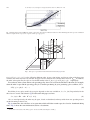
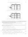
Tema 1: Modelación y Calibración de Procesos Estocásticos para Precios de Instrumentos
en Mercados con Paneles de Datos Incompletos.
Discusión:
Se perfecciona metodología cuya investigación se inició en fecha anterior al inicio del proyecto
(financiado parcialmente por proyecto Fondef D00I1024) orientado a cómo determinar la mejor
curva de precios de hoy (y su dinámica a través del tiempo) en presencia de un número limitado
de precios producto de la falta de liquidez del mercado.
La estrategia propuesta consiste en calibrar un modelo multifactorial para la dinámica de los
precios y utilizar filtros de Kalman calibrados con paneles incompletos.
Publicaciones
Cortazar, G, Schwartz, E. S., Naranjo, L, (2007) "Term Structure Estimation in Markets with Infrequent Trading“
International Journal of Finance and Economics (por aparecer)
Cortazar, G., Naranjo, L. (2006) “An N-Factor Gaussian Model of Oil Futures Prices” The Journal of Futures
Markets, Vol.26, No. 3, March, 2006, 243-268
Presentaciones en Congresos Académicos
Cortazar, G, Schwartz, E. S., Naranjo, L, (2006) "Term Structure Estimation in Markets with Infrequent Trading".
Latin American Meeting of the Econometric Society (LAMES) , ITAM, Ciudad de México, Nov. 2-4, 2006
Cortazar, G, Schwartz, E. S., Naranjo, L, (2006) "Term Structure Estimation in Markets with Infrequent Trading".
2006 FMA Annual Meeting , Salt Lake City, Oct. 11 - 14, 2006
Cortazar, G, Schwartz, E. S., Naranjo, L, (2006) "Term Structure Estimation in Markets with Infrequent Trading".
2006 Far Eastern Meeting of the Econometric Society, Beijing, July 9-12, 2006
Cortazar, G, Schwartz, E. S., Naranjo, L, (2006) "Term Structure Estimation in Markets with Infrequent Trading".
15th annual meeting of the European Financial Management Association, Madrid, June 28-July 1, 2006
Cortazar, G., Naranjo, L. (2005) “An N-Factor Gaussian Model of Oil Futures Prices” 2005 FMA Annual Meeting,
Chicago, October 12-15, http://www.fma.org/Chicago/ChicagoProgram.htm
Cortazar, G, Schwartz, E. S., Naranjo, L, (2004) "Term Structure Estimation in Low-Frequency Transaction
Markets: A Kalman Filter Approach with Incomplete Panel-Data" (March 2004). EFA 2004 Maastricht Meetings
Paper No. 3102. , Maastricht, August 18-21, http://ssrn.com/abstract=567090
Tema 2: Metodologías de Valorización de Derivados escritos sobre Subyacentes con
procesos Completos
Discusión:
Aún cuando existen múltiples procedimientos para valorizar opciones de tipo Americano (cuya
estrategia óptima de ejercicio no es evidente), la complejidad para su implementación crece
exponencialmente con la dimensión del problema a resolver. Dado que los modelos de precios
actuales requeridos para representar adecuadamente la dinámica de tasas de interés y de precios
son multifactoriales, estas metodologías tradicionales son en la práctica inutilizables para
valorizar los activos derivados escritos sobre estas tasas de interés o precios.
La estrategia de resolución propuesta consiste en adaptar metodologías recientes que usan un
método que combina simulación de Montecarlo (forward) con resolución backward de árboles
construidos a partir de estas simulaciones.
Publicaciones
Cortazar, G., Gravet, M., Urzua, J. (2008) “The Valuation of Multidimensional American Real Options using the
LSM Simulation Method” Computers & Operations Research Vol 35 (2008) 113 – 129
Presentaciones en Congresos Académicos
Cortazar, G., Gravet, M., Urzua, J. (2005) “The Valuation of Multidimensional American Real Options using the
LSM Simulation Method”, 9th Annual International Conference Real Options: Theory Meets Practice, Real Options
Group and EDC Paris, Paris, June 23-25, http://www.realoptions.org/AcademicProgram/academicprogram2005.html
Tema 3: Metodologías de Medición de Spreads.
Discusión:
Existen diversos tipos de spreads o diferenciales de precios (o tasas) entre los activos más
deseados por el mercado (los que se transan a mayores precios, o equivalentemente descontados a
las menores tasas) y el resto. Este diferencial se puede deber a la existencia de riesgos de crédito
o de liquidez que explican que inversionistas racionales sólo los adquieren en la medida que se
transen a un descuento relativo los “mejores” activos del mercado.
Durante la realización del proyecto se desarrollaron metodologías de estimación de spreads para
diversos instrumentos de deuda (bonos de empresas, letras hipotecarias, depósitos a plazo, Bonos
de Reconocimiento, etc) así como estimaciones de los spreads de liquidez presentes entre activos
de la misma familia (Bonos Banco Central) pero que exhiben distinta liquidez (ej PRC 8 años
versus PRC a 10 años).
Tesis de Magíster
“Estimación de Spreads por Liquidez en un Mercado con Pocas Transacciones: El Caso del Mercado de Bonos del
Banco Central de Chile”, PEDRO MATÍAS MORAL MESA, Tesis de Magíster en Ciencias de la Ingeniería,
Pontificia Universidad Católica de Chile, 17-01-2006
Memorias de Título
“Bonos Corporativos: una Revisión del Mercado y una Aproximación a un Método Práctico de Valorización” ,
Memoria Escuela de Ingeniería, Pontificia Universidad Católica de Chile, CLAUDIO EDUARDO HELFMANN
SOTO , 31-12-2005
“Valorización de Instrumentos Financieros en Mercados con Pocas Transacciones: Análisis de una Metodología
Basada en un Modelo Dinámico para la Tasa Cero Real en Chile” JOSE LUIS MANIEU ESPINOSA, Memoria
Escuela de Ingeniería, Pontificia Universidad Católica de Chile 12-08-2005
Tema 4: Metodologías de Medición de Riesgos y de Asignación de Activos (Asset Allocation)
para Carteras de Inversión
Existe una extensa literatura de cómo medir los riesgos financieros en una cartera e inversión
(Value at Riks, Tracking error, etc) y de cómo tomar decisiones de Asignación de Activos (Asset
Allocation) que permitan mejorar el proceso de inversiones.
Sin embargo, para poder resolver estos problemas en mercados emergentes como el chileno, con
ausencia de transacciones hace falta modificar procedimientos y generar información confiable
relativa al comportamiento de las distintas clases de activos, entre otros aspectos.
Documentos de Trabajo aún no publicados
Cortazar, G, Bernales, A. Beuermann, D. (2007) “Methodology and Implementation of Value-at-Risk Measures
in Emerging Fixed-Income Markets with Infrequent Trading
Tesis de Magíster
“Estimación de Spreads por Liquidez en un Mercado con Pocas Transacciones: El Caso del Mercado de Bonos del
Banco Central de Chile”, PEDRO MATÍAS MORAL MESA, Tesis de Magíster en Ciencias de la Ingeniería,
Pontificia Universidad Católica de Chile, 17-01-2006
“Metodología e Implementación de Métodos de VALUE AT RISK en Mercados de Renta Fija con baja Frecuencia
de Transacciones” ALEJANDRO ADRIAN BERNALES SILVA, Tesis de Magíster en Ciencias de la Ingeniería,
Pontificia Universidad Católica de Chile, 23-12-2005
Memorias de Título
“Decisiones de Asset Allocation en Carteras de Inversión de las AFP: Aplicación del Modelo de Black &
Litterman”, RODRIGO ALFONSO IBANEZ VILLARROEL, Memoria Escuela de Ingeniería, Pontificia
Universidad Católica de Chile, 26-07-2005
Tema 5: Modelación y Calibración Conjunta de Procesos Estocásticos de Múltiples Activos.
Durante el desarrollo del proyecto se hizo evidente que en algunas situaciones se hace
conveniente utilizar información de precios de ciertos instrumentos financieros para estimar de
mejor manera el precio de otro instrumento que no fue transado, pero que históricamente ha
exhibido retornos correlacionados parcialmente entré sí.
El inicio de esta línea de investigación está siendo muy prometedora permitiendo mejorar
sustancialmente los modelos para la dinámica de precios que inicialmente consideraban sólo una
familia de instrumentos.
Documentos de Trabajo aún no publicados
Cortazar, G, Milla, C. Severino, F. (2007) “A Multicommodity Model of Futures Prices: Using Futures Prices of One
Commodity to Estimate the Stochastic Process of Another”
Tesis de Magíster
"Modelo estocástico multicommodity para la dinámica de precios de contratos futuros. Selección y estimación del
modelo utilizando componentes principales comunes y filtro de Kalman", FELIPE SEVERINO DIAZ, Tesis de
Magíster en Ciencias de la Ingeniería, Pontificia Universidad Católica de Chile, 26-03-2007
“Estimación de Spreads por Liquidez en un Mercado con Pocas Transacciones: El Caso del Mercado de Bonos del
Banco Central de Chile”, PEDRO MATÍAS MORAL MESA, Tesis de Magíster en Ciencias de la Ingeniería,
Pontificia Universidad Católica de Chile, 17-01-2006
“Modelos Estocásticos de Precios de Commodities y Estimación Conjunta de la Dinámica de dos Commodities
Mediante el Filtro de Kalman” CARLOS IGNACIO MILLA GONZALEZ, Tesis de Magíster en Ciencias de la
Ingeniería, Pontificia Universidad Católica de Chile, 23-12-2005
Presentaciones en Congresos Académicos
Cortazar, G, Milla, C. Severino, F. (2007) “A Multicommodity Model of Futures Prices: Using Futures Prices of One
Commodity to Estimate the Stochastic Process of Another”,4th Annual Conference of Asia Pacific Association of
Derivatives (APAD), Gurgaon, India, June 20-22, 2007
3.
OTROS INFORMES TÉCNICOS
4.
EVALUACIÓN CIENTÍFICO-TECNOLÓGICA
A continuación se resume un análisis FODA del proyecto
Fortalezas del Proyecto
-Las metodologías científicas desarrolladas para abordar ausencia de transacciones
-La plataforma tecnológica-computacional incluyendo rutinas computacionales y plataforma
WEB.
-Las bases de datos construidas
-El equipo humano especializado capacitado
-La reputación en el mercado
Debilidades del Proyecto
-La vulnerabilidad financiera que lo expone a ataques de eventuales competidores que inicien una
guerra de precios.
-Exigencia de mantener innovación permanente como protección de mercado.
Oportunidades del Proyecto
-Posibilidades de expansión internacional.
Amenazas
-Entrada de competencia nacional e internacional.
5.
EVALUACIÓN ECONÓMICO-SOCIAL
Análisis comparativo con la evaluación ex-ante de la Formulación del Proyecto.
A continuación se discute y actualiza la evaluación económico social presentada en la
Formulación del Proyecto.
Tal como se plantea en la Formulación del proyecto, el beneficio social principal de este
proyecto se genera al contribuir a la modernización del mercado financiero nacional. Un
resultado exitoso en cuanto a nuevas herramientas de gestión de carteras, como es el caso de lo
ocurrido con este proyecto debiera inducir que las administradoras de fondos de pensiones,
pueden mejorar la gestión de sus carteras y de esta manera obtener mayores retornos de sus
inversiones, sin incrementar el riesgo asumido.
El principal impacto económico social del proyecto es el Incremento Marginal de la
Rentabilidad aplicado a una Fracción de los Fondos Potenciales que pudieran verse
beneficiados con las herramientas de gestión de carteras desarrolladas. Por último, se debe
estimar el adelantamiento de los flujos (en número de años) que representa la realización del
proyecto comparado con la situación base sin proyecto (i.e. se estima que si no hubiera habido
proyecto, otro similar se hubiera desarrollado teniendo el mismo impacto después).
Los cuatro parámetros anteriores son difíciles de estimar y de ellos depende el resultado de los
indicadores económicos-sociales.
En la Evaluación ex–ante presentada en la formulación del proyecto se asumieron los
siguientes valores para estos parámetros:
Incremento Marginal de la Rentabilidad = 0,25%
Fracción = 25% de las administradoras* 60% de los activos = 15%
Fondos Potenciales = MMUS$ 40.000
Adelantamiento = 1 año (si no se hace el proyecto los flujos se realizan 1 año después).
Con lo que el beneficio económico-social por año se estimó en US$ 15 millones y los flujos
netos del proyecto presentados en su Formulación bajo estos supuestos fueron:
.
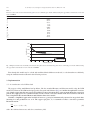
FLUJO NETO
Ingresos
Costos
Inversión
Costo total I+D
Fondef
Beneficio neto
TIR
VAN (10%) MM$
VAN/VAI
VAN/FONDEF
0
0
0
290
97
-290
0
0
-509
219
97
290
10.754
276
-509
0
0
10.987
238
136
-6
0
0
108
238
136
-6
119
70
-6
119
71
-6
0
38
-6
0
38
-6
0
0
-6
108
55
54
-32
-32
6
568,06%
9.244
18,90
50,14
Nota: M/N = moneda nacional
M/E = moneda extranjera
Como se planteó anteriormente, la estimación de los parámetros anteriores está sujeta a
bastante incertidumbre. Sin embargo se puede señalar que desde la formulación del proyecto
uno de los parámetros se ha incrementado significativamente, al aumentar el parámetro
Fondos Potenciales subió al año 2007 a más de MM US$100.000, es decir 2,5 veces mayor
que el valor estimado en la Formulación. Esto permitiría dividir por 2,5 alguno de los
indicadores anteriores (por ejemplo suponer que el Incremento Marginal de la Rentabilidad
fuera 0,1 en vez de los 0,25 asumidos originalmente) y conservar el valor de los indicadores
originales.
Debido a lo anterior, una evaluación conservadora mantendría los indicadores económicosociales presentados en la Formulación inicial.
DESCRIPCION DE LA SITUACION SIN PROYECTO
Para analizar la situación sin proyecto, se ha hecho el supuesto que en caso de no realizarse este
proyecto, otro con similares objetivos, pero sin algunas de las sinergias presentes en este proyecto, se
desarrollaría con un retraso de sólo un año. Este supuesto de evaluación busca reflejar la dinámica actual
de modernización financiera que está teniendo el mercado, que si bien está convergiendo a los
estándares de mercados desarrollados, en algunas áreas como las que aborda este proyecto no lo hace
con suficiente velocidad.
No se está condicionando la modernización del sistema chileno a este proyecto, sino que se está
suponiendo que al hacerlo se adelantan los resultados con el consecuente beneficio para los usuarios.
La evaluación considera que tanto los ingresos como los costos obtenidos por este desarrollo privado son
equivalentes a la situación con proyecto, pero que se obtienen un año después. Además la inversión
inicial es superior, ya que para obtener los sistemas adecuados, estos deben ser adquiridos y
desarrollados por consultores externos en el extranjero quienes deben estudiar el comportamiento del
mercado nacional para luego desarrollar desde cero los productos.
DESCRIPCION DE LA SITUACION CON PROYECTO
La situación con proyecto considera que el proyecto adelanta los beneficios económicos-sociales y que el
costo de desarrollo es menor en este proyecto que en su eventual competencia.
MEMORIA DE CÁLCULO DE LA EVALUACIÓN ECONÓMICO-SOCIAL
SIN PROYECTO
(La información aquí contenida se extrae de la hoja "SITUACION SIN PYTO")
En millones de pesos
Variables Críticas
Unidad (m3, kg, l, ton, etc.)
Valor Escenario Pesimista
Valor Escenario Optimista
Valor Más Probable
AÑO
Var. 1
Var. 2
%
%
Var. 3
%
Descripción Variable 1:
Porcentaje de Rentabilidad Adicional Anual de Fondos de Pensiones
0,10%
20%
50%
Descripción Variable 2:
Porcentaje de Cartera Administrada que es impactada por nuevas tecnologías de Gestión Optima de Cateras
0,50%
50%
100%
Descripción Variable 3:
Porcentaje de Activos en Cartera que es impactada por nuevas tecnologías de Gestión Optima de Cateras
0,25%
25%
60%
1
2
3
4
5
6
7
8
9
10
INGRESOS
Moneda nacional
Moneda extranjera equivalente
Total ingresos
0
0
0
0
0
0
0
0
0
297
10457
10754
535
10457
10991
772
10457
11229
891
10457
11348
1010
10457
11466
1069
10457
11526
1129
10457
11585
COSTOS
Mano de obra calificada
Mano de obra no calificada
Insumos (M/N)
Bienes de capital (M/N)
Otros (M/N)
Total costos
0
0
0
0
0
0
0
0
0
0
0
0
0
0
0
0
0
0
226
0
24
14
12
276
357
0
26
15
13
412
487
0
29
17
15
548
552
0
32
19
16
618
616
0
35
20
18
689
646
0
39
23
19
727
676
0
43
25
21
765
INVERSIONES
En moneda nacional
En moneda extranjera
Total inversiones
0
0
0
509
0
509
509
0
509
6
0
6
6
0
6
6
0
6
6
0
6
6
0
6
6
0
6
6
0
6
BENEFICIOS
0
-509
-509
10472
10573
10675
10723
10772
10793
10815
CON PROYECTO
(La información aquí contenida se extrae de la hoja "SITUACION CON PYTO")
En millones de pesos
Variables Críticas
Unidad (m3, kg, l, ton, etc.)
Valor Escenario Pesimista
Valor Escenario Optimista
Valor Más Probable
AÑO
Var. 1
Var. 2
%
%
Var. 3
%
0,10%
20%
50%
Descripción Variable 1:
Porcentaje de Rentabilidad Adicional Anual de Fondos de Pensiones
0,50%
50%
100%
Descripción Variable 2:
Porcentaje de Cartera Administrada que es impactada por nuevas tecnologías de Gestión Optima de Cateras
0,25%
25%
60%
Descripción Variable 3:
Porcentaje de Activos en Cartera que es impactada por nuevas tecnologías de Gestión Optima de Cateras
1
2
3
4
5
6
7
8
9
10
INGRESOS
Ingresos por ventas
Externalidad Positiva 1
Total ingresos
0
0
0
0
0
0
297
10457
10.754
COSTOS
Mano de obra calificada
Mano de obra no calificada
Insumos (M/N)
Bienes de capital (M/N)
Otros (M/N)
Total costos
0
0
0
0
0
0
0
0
0
0
0
0
226
0
24
14
12
276
357
0
26
15
13
412
487
0
29
17
15
548
552
0
32
19
16
618
616
0
35
20
18
689
646
0
39
23
19
727
676
0
43
25
21
765
676
0
43
25
21
765
INVERSIONES
En moneda nacional
En moneda extranjera
Total inversiones
0
0
0
0
0
0
0
0
0
0
0
0
0
0
0
0
0
0
0
0
0
0
0
0
0
0
0
0
0
0
290
0
290
97
219
0
219
97
0
0
0
0
0
0
0
0
-290
-219
10.478
0
0
0
290
97
-290
0
0
-509
219
97
290
10.754
276
-509
0
0
10.987
COSTO I&D (parciales por año)
En M/N
En M/E
Total I&D (todos los aportes)
Sólo lo solicitado a FONDEF
BENEFICIOS
535
772
891
1010
1010
1069
1129
10457 10457 10457 10457 10457 10457 10457
10.991 11.229 11.348 11.466 11.466 11.526 11.585
10.579 10.681 10.729 10.778 10.740 10.761 10.821
FLUJO NETO
Ingresos
Costos
Inversión
Costo total I+D
Fondef
Beneficio neto
TIR
VAN (10%) MM$
VAN/VAI
VAN/FONDEF
Nota: M/N = moneda nacional
M/E = moneda extranjera
568,06%
9.244
18,90
50,14
238
136
-6
0
0
108
238
136
-6
119
70
-6
119
71
-6
0
38
-6
0
38
-6
0
0
-6
108
55
54
-32
-32
6
SITUACION SIN PROYECTO
(Situación para primer año de actividades)
MERCADO SITUACION SIN PROYECTO (Para cada Producto o Servicio a evaluar)
AÑO
0
1
2
3
4
5
6
7
Mercado Sin Proyecto.
Producto o Sevicio 1
(Unidades)
0
0
0
0
5
9
13
15
AÑO
8
9
10
Mercado Sin Proyecto.
Producto o Servicio 1
(Unidades)
17
18
19
Moneda
Pesos
Tipo de cambio $
$697
Cantidad anual
Mercado Nacional
(Unidades)
Cantidad anual
Mercado Export.
(Unidades)
Ingresos Mercado
Nacional (MM$)
Ingresos Mercado
Exportador (MM$)
Total de Ingresos
(MM$)
5
0
0
0
0
0
297
0
0
0
0
0
$297
$0
$0
5
0
297
0
297
INGRESOS
Productos o servicios
1
2
n
Tipo de unidad a
considerar
Precio Unitario
Servicios a Usuarios
($)
59400000
0
0
TOTAL INGRESOS
COSTOS
MANO DE OBRA CALIFICADA
Nº Puestos
Cargos
Costo mensual
unitario $
Costo total mensual
(MM$)
Costo total anual
(MM$)
1
7
5
3
0
Gerente
Profesional
Tecnico
Administrativo
Otros (definir)
4000000
1350000
750000
550000
0
4
9,45
3,75
1,65
0
48
113,4
45
19,8
0
18,85
226,2
Costo mensual
unitario $
Costo total mensual
(MM$)
Costo total anual
(MM$)
0
0
0
0
0
0
0
0
TOTALES
MANO DE OBRA NO CALIFICADA
Nº Puestos
Cargos
0
0
Obreros y Jornaleros
Otros (definir)
TOTALES
INSUMOS PARA LA PRODUCCION
Insumos para la
producción
Tipo de unidad a
considerar
Costo Unitario
($)
Cantidad mensual
(Unidades)
Costo total mensual
(MM$)
Costo total anual
(MM$)
1
Insumos de Oficina
Promedio
500000
4
2
24
0
0
0
0
0
0
0
0
2
24
2
3
TOTALES
BIENES DE CAPITAL
Bienes de Capital
1
2
3
Moneda
Tipo de unidad a
considerar
Cantidad
N° computadores
Mantención Oficinas
8
10
0
Tipo de cambio $
Costo Unitario
($)
500000
1000000
0
TOTALES
Costo total anual
(MM$)
4
10
0
14
OTROS COSTOS
Otros costos
1
2
3
Tipo de unidad a
considerar
Costo Unitario
($)
Cantidad mensual
(Unidades)
Costo total mensual
(MM$)
Costo total anual
(MM$)
Arriendo Mensual
1000000
0
0
1
0
0
1
0
0
12
0
0
1
12
TOTALES
$276
TOTAL COSTOS ANUALES
RESUMEN DE INVERSIONES
ITEM
Terreno
Infraestructura física
Maquinaria y equipos
Otros (definir)
TOTAL
EN MONEDA
NACIONAL (MM$)
0
0
0
1018
1018
EN MONEDA
EXTRANJERA (MM$)
0
0
0
0
0
TOTAL GENERAL
(MM$)
0
0
0
1018
1018
SITUACION CON PROYECTO
(Situación para primer año de actividades)
CURVA DE ADOPCION DE LA TECNOLOGIA (Para cada Producto o Servicio)
AÑO
Mercado Con
Proyecto
Producto 1
(Unidades)
AÑO
Mercado Con
Proyecto
Producto 1
(Unidades)
0
1
2
3
4
5
6
7
0
0
0
5
9
13
15
17
8
9
10
17
18
19
INGRESOS
Moneda Extranjera
Productos o
servicios
Tipo de unidad a
considerar
1
Servicios a Usuarios
2
n
Tipo de cambio $
Cantidad anual
Mercado Nacional
(Unidades)
Cantidad anual
Mercado Export.
(Unidades)
Ingresos Moneda
Nacional (MM$)
Ingresos Moneda
Extranjera (MM$)
Total de Ingresos
(MM$)
59400000
5
0
297
0
$297
0
0
0
0
0
0
0
0
0
0
$0
$0
5
0
297
0
297
Precio Unitario
($)
TOTAL
COSTOS
Moneda Extranjera
MANO DE OBRA CALIFICADA
Tipo de cambio $
(Para todos los productos y todas las Unidades de Negocio)
Nº Puestos
Cargos
Costo mensual
unitario $
Costo total mensual
(MM$)
Costo total anual
Moneda Nacional
(MM$)
Costo total anual
Moneda Extranjera
(MM$)
1
Gerente
4000000
4
48
0
7
Profesional
1350000
9,45
113,4
0
5
Tecnico
750000
3,75
45
0
3
0
Administrativo
Otros (definir)
550000
0
1,65
0
19,8
0
0
0
18,85
226,2
0
TOTALES
Moneda Extranjera
MANO DE OBRA NO CALIFICADA
Tipo de cambio $
(Para todos los productos y todas las Unidades de Negocio)
Nº Puestos
Cargos
0 Obreros y Jornaleros
0
Otros (definir)
TOTALES
Costo mensual
unitario $
Costo total mensual
(MM$)
Costo total anual
Moneda Nacional
(MM$)
Costo total anual
Moneda Extranjera
(MM$)
0
0
0
0
0
0
0
0
0
0
0
Moneda Extranjera
INSUMOS PARA LA PRODUCCION
Tipo de cambio $
(Para todos los productos y todas las Unidades de Negocio)
Insumos para la
producción
Tipo de unidad a
considerar
Costo Unitario
($)
Cantidad mensual
(Unidades)
Costo total mensual
(MM$)
Costo total anual
Moneda Nacional
(MM$)
Costo total anual
Moneda Extranjera
(MM$)
1
Insumos de Oficina
Promedio
500000
4
2
24
0
0
0
0
0
0
0
0
0
0
0
2
24
0
2
3
TOTALES
Moneda Extranjera
BIENES DE CAPITAL
Tipo de cambio $
(Para todos los Productos y todas las Unidades de Negocio)
Bienes de
Capital
Tipo de unidad a
considerar
Cantidad
1
N° computadores
8
2
3
Mantención Oficinas
10
0
Costo total anual
Moneda Nacional
(MM$)
Costo total anual
Moneda extranjera
(MM$)
500000
4
0
1000000
0
10
0
0
0
14
0
Costo Unitario
($)
TOTALES
Moneda Extranjera
OTROS COSTOS
Tipo de cambio $
(Para todos los Productos y todas las Unidades de Negocio)
Otros costos
Tipo de unidad a
considerar
Cantidad
1
Arriendo Mensual
12
0
0
2
3
Costo total anual
Moneda Nacional
(MM$)
Costo total anual
Moneda Extranjera
(MM$)
1000000
12
0
0
0
0
0
0
0
12
0
Costo Unitario
$
TOTALES
$276
TOTAL COSTOS ANUALES MONEDA NACIONAL (MM$)
RESUMEN DE INVERSIONES
ITEM
EN MONEDA
EN MONEDA
TOTAL GENERAL
NACIONAL (MM$)
EXTRANJERA (MM$)
(MM$)
Terreno
0
0
0
Infraestructura física
0
0
0
Maquinaria y equipos
0
0
0
Otros (definir)
509
0
509
TOTAL
509
0
509
FUENTE DE
FINANCIAMIENTO
EN MONEDA
NACIONAL
EN MONEDA
EXTRANJERA
TOTAL
FONDEF
123
0
123
INSTITUCIONES
EMPRESAS Y OTRAS
ENTIDADES
228
0
228
158
0
158
TOTAL
509
0
509
COSTO PROYECTO I+D
PARTE V
ANEXOS
ANEXO 1.
PLAN DE NEGOCIOS
A continuación se describen los principales aspectos del Plan de Negocios en ejecución:
4.1 Productos
Se considera la comercialización de 3 servicios independiente. Cada uno de ellos se distribuye
via Internet como módulos independientes de la plataforma RiskAmerica, la que al incluir estos
nuevos módulos se distribuye bajo el nombre de RiskAmericaPlus.
Los 3 Módulos de Servicios ofrecidos son:
4.1.1 Módulo SVC
El SVC o Sistema de Valorización de Carteras consiste en un módulo del servicio
RiskAmericaPlus cuyo objetivo es asignarle una TIR a cada nemotécnico solicitado.
El usuario envía vía Web un archivo indicando los nemotécnicos asociados a su cartera,
devolviendo el sistema la TIR que el modelo le asigna a cada uno. La TIR del modelo depende
de si el activo fue transado ese día, de cuál es la curva de referencia para el día (la que es
actualizada diariamente) y de la historia de spreads que este nemotécnico ha exhibido respecto de
la curva en el pasado.
4.1.2 Módulo Índices
Este módulo entrega información referida al comportamiento del mercado financiero. Esta
descripción se realiza en términos de distintas familias y clases de activos, incluyéndose tanto
renta fija como variable.
Para cada uno de los más de 100 índices existentes se entrega información de su composición así
como de su comportamiento en términos de retornos y riesgos.
Asimismo, se pueden comparar y realizar análisis entre los distintos índices:
Se entrega además la posibilidad de construir y índices personalizados:
También se pueden cargar índices generados externamente:
4.1.2 Módulo Portfolio
Este módulo entrega información de de riesgo, retorno y performance tanto de carteras existentes
del mercado, como de carteras propias.
En Información de Mercado entrega información información de riesgo, de retornos y de
performance de carteras públicas de AFP y de Fondos Mutuos, como se muestra en las siguientes
páginas web:
En Riesgo Absoluto se entregan herramientas para calcular el Value-at-Risk de carteras propias
tanto por métodos paramétricos como por simulación histórica.
En Riesgo Relativo se entregan herramientas para calcular el Tracking Error y el VaR Relativo a
entre dos carteras.
En Asset Allocation se entregan herramientas para calcular carteras con combinaciones riesgoretorno óptimas.
En Análisis de Desempeño se entregan herramientas para calcular carteras el performance de
carteras definidas por el usuario.
4.2 Clientes
Los clientes potenciales para los resultados de este proyecto son principalmente instituciones
financieras a las que se pueden agregar sus instituciones reguladoras. A continuación se entrega
una lista actualizada de los clientes potenciales provenientes de AFP, Fondos Mutuos, Bancos,
Cias de Seguros. A estas listas habría que agregar corredoras de bolsa, securitizadoras,
proveedores de diversos servicios financieros e instituciones reguladoras.
Tipo
AFP
Nombre
Bansander S.A.
Cuprum S.A.
Habitat S.A.
Planvital S.A.
Provida S.A.
Santa María S.A.
Tipo
Nombre
Administradoras de Administradora General de Fondos Security S.A.
Fondos Mutuos
Banchile Administradora General de Fondos S.A.
BancoEstado S.A. Administradora General de Fondos
Bandesarrollo Administradora General de Fondos S.A.
BBVA Administradora General de Fondos S.A.
BCI Administradora de Fondos Mutuos S.A.
BICE Administradora General de Fondos S.A.
Boston Administradora General de Fondos S.A.
Celfín Capital S.A. Administradora General de Fondos
Consorcio S.A. Administradora General de Fondos
Corp Banca Administradora General de Fondos S.A.
Cruz del Sur Administradora General de Fondos S.A.
Euroamérica Administradora General de Fondos S.A.
IM Trust S.A. Administradora General de Fondos
Larraín Vial Administradora General de Fondos S.A.
Legg Mason (Chile) Administradora General de Fondos S.A.
Penta Administradora General de Fondos S.A.
Principal Administradora General de Fondos S.A.
Santander Santiago S.A. Administradora General de Fondos
Scotia Sudamericano Administradora de Fondos Mutuos S.A.
Zurich Administradora General de Fondos S.A.
Tipo
Banco
Tipo
Seguros
Nombre
ABN AMRO Bank
Banco BICE
Banco de Chile
Banco de Crédito e Inversiones
Banco de la Nación Argentina
Banco del Desarrollo
Banco del Estado de Chile
Banco do Brasil
Banco Falabella
Banco Internacional
Banco Paris
Banco Penta
Banco Ripley
Banco Santander Santiago
Banco Security
BankBoston
BBVA
Citibank N.A.
CorpBanca
Deutsche Bank
HNS Banco
HSBC Bank Chile
JPMorgan Chase Bank
Scotiabank Sud Americano
The Bank of Tokyo-Mitsubishi Ltd.
Nombre
Aseguradora Magallanes
BICE Vida
Cardif
Chilena Consolidada
COFACE
Consorcio Nacional
Continental
Corredora Security S.A.
Cruz del Sur
Eurovida
ING
Interamericana
ISE
Liberty
MAPFRE
Mutual de Carabineros
Mutual de Seguros de Chile
Renta Nacional
Royal & Sunalliance
Seguros de Vida la Construcción SA
4.3 Factores de Éxito
El principal Factor de Éxito es la capacidad de generar y comunicar una reputación de
objetividad, rigurosidad y compromiso de permanente innovación para los Servicios ofrecidos.
Para ello se hace necesario mantener activo un equipo de investigadores haciendo investigación
reconocida internacionalmente.
Es en este contexto que independientemente de la evolución comercial de RiskAmerica, ésta se
debe mantener ligada estrechamente a la investigación académica que se realiza en la Pontificia
Universidad Católica de Chile a través del FINlabUC-Laboratorio de Investigación Avanzada en
Finanzas.
4.4 Comercialización
La distribución de los resultados se realizará a través de la plataforma WEB RiskAmerica, la que
comunicó al mercado la incorporación de estos servicios expandidos como RiskAmericaPlus.
Asimismo se deben intensificar el plan de contactos, comunicación y capacitación de usuarios
potenciales a través de encuentros y presentaciones y distribución de material gráfico.
Adicionalmente se debe seguir explorando oportunidades de internacionalización de los servicios.
A continuación se entrega copia parcial de material desarrollado.
4.5 Ventas Actuales y Proyección de Resultados Futuros
Las ventas esperadas de los 3 módulos de Servicios para el año 2007 alcanzan MM$198
las que debieran incrementarse en los años futuros hasta alcanzar un monto esperado de MM$570
el año 2010.
A continuación se presentan los ingresos y egresos proyectados por los próximos 7 años,
así como el VAN de los excedentes descontados al 12% anual.
En forma muy conservadora, no se supone valor residual alguno.
Se estima un VAN al 12% de MM$781,6 para la explotación comercial de los resultados
del proyecto
Montos en MM$
Mod-SVC
Mod-Indices
Mod-Portfolio
Total Ing
Costos Fijos
Costos Variables
Total Costos
Excedentes
VAN(12%)
2007
180
10
8
198
120
65,34
185,34
12,66
781,6
2008
200,0
47,0
75,0
322
120
106,26
226,26
95,74
2009
220,0
85,0
142,0
447
120
147,51
267,51
179,49
2010
240
120
210
570
120
188,1
308,1
261,9
2011
240
120
210
570
120
188,1
308,1
261,9
2012
240
120
210
570
120
188,1
308,1
261,9
2013
240
120
210
570
120
188,1
308,1
261,9
ANEXO 2. PLANES DE TRABAJO INICIAL Y EFECTIVAMENTE EJECUTADO
Tipo
Convenios Contraparte :
2 Convenios Con
Contrapartes
Plan de Experimentos
definido :
19 Plan De Experimentos
Definido A
Www.riskportfolio
Diseño de Prototipo
19 emitido :
Diseno De Pagina Web
Experimentos Críticos
Efectuados :
19 Experimentos Criticos
Efectuados
Www.riskportfolio
Prototipo Probado a nivel
Laboratorio :
19 Prototipo
Www.riskportfolio Probado
A Nivel Laboratorio
Prototipo probado a Nivel
19 Piloto/Planta :
Www.riskportfolio.comv1
Diseño de Prototipo
27 emitido :
Diseno De
Assetallocationv1
Plan de Experimentos
definido :
27 Plan De Experimentos
Definido Para
Assetallocation
Experimentos Críticos
27 Efectuados :
Experimentos Criticos
Efectuados Assetallocation
Prototipo Probado a nivel
27 Laboratorio :
Prototipo Probado A Nivel
Laboratorio Assetallocation
Prototipo probado a Nivel
27 Piloto/Planta :
Assetallocationv1
Plan de Experimentos
29 definido :
Plan De Experimentos
Definido Riskmatrix
Nombre Resultado
Programada
Reprogramada
Fechas
Lograda
06/03/2005
06/04/2005
06/04/2005
30/06/2005
30/06/2005
30/06/2005
30/06/2005
30/06/2005
30/06/2005
30/06/2005
15/09/2005
15/09/2005
30/06/2005
30/09/2005
30/09/2005
30/06/2005
30/09/2005
30/09/2005
01/08/2005
01/08/2005
01/08/2005
15/08/2005
15/08/2005
15/08/2005
25/08/2005
25/08/2005
25/08/2005
30/09/2005
30/09/2005
30/09/2005
30/09/2005
30/09/2005
30/09/2005
15/10/2005
15/10/2005
15/10/2005
Descripción
Plan de Experimentos
21 definido :
Plan De Experimentos
Definido Portfoliovalue
Experimentos Críticos
21 Efectuados :
Experimentos Criticos
Efectuados Portfoliovalue
Experimentos Críticos
29 Efectuados :
Experimentos Criticos
Efectuados Riskmatrix
Diseño de Prototipo
29 emitido :
Diseno De Riskmatrixv1
Diseño de Prototipo
21 emitido :
Diseno De Portfoliovaluev1
Prototipo Probado a nivel
21 Laboratorio :
Prototipo Probado A Nivel
Laboratorio Portfoliovalue
Prototipo probado a Nivel
21 Piloto/Planta :
Portfoliovaluev1
Prototipo probado a Nivel
29 Piloto/Planta :
Riskmatrixv1
Prototipo Probado a nivel
29 Laboratorio :
Prototipo Probado A Nivel
Laboratorio Riskmatrix
Plan de Experimentos
definido :
25 Plan De Experimentos
Definido
Portfoliobenchmarks
Plan de Experimentos
23 definido :
Plan De Experimentos
Definido Portfoliorisk
Experimentos Críticos
Efectuados :
25 Experimentos Criticos
Efectuados
Portfoliobenchmarks
Experimentos Críticos
23 Efectuados :
Experimentos Criticos
Efectuados Portfoliorisk
25 Diseño de Prototipo
emitido :
15/10/2005
15/10/2005
15/10/2005
25/10/2005
25/10/2005
25/10/2005
25/10/2005
25/10/2005
25/10/2005
30/10/2005
30/10/2005
30/10/2005
30/10/2005
30/10/2005
30/10/2005
30/12/2005
15/03/2006
23/01/2006
30/12/2005
15/03/2006
23/01/2006
30/12/2005
30/12/2006
30/12/2006
30/12/2005
30/12/2006
30/12/2006
15/04/2006
15/04/2006
28/04/2006
15/04/2006
15/06/2006
15/06/2006
25/04/2006
25/04/2006
28/04/2006
25/04/2006
30/06/2006
30/06/2006
30/04/2006
30/04/2006
28/04/2006
Diseno De
Portfoliobenchmarksv1
Diseño de Prototipo
23 emitido :
Diseno De Portfolioriskv1
30/04/2006
30/07/2006
30/06/2006
30/06/2006
30/06/2006
30/06/2006
30/06/2006
30/06/2006
30/06/2006
30/06/2006
30/06/2006
30/06/2006
30/06/2006
30/06/2006
30/06/2006
30/06/2006
30/06/2006
30/06/2006
30/06/2006
30/08/2006
01/08/2006
30/06/2006
30/12/2006
10/01/2007
30/06/2006
02/01/2007
02/01/2007
15/12/2006
30/12/2006
30/12/2006
25/12/2006
30/12/2006
20/01/2007
16 Tesís :
2 Tesis De Pregrado
30/12/2006
30/12/2006
31/12/2005
15 Tesís :
Tesis De Magister
30/12/2006
30/12/2006
17/01/2006
Diseño de Prototipo
31 emitido :
Diseno De
Productofinalriskportfoliov2
30/12/2006
30/12/2006
20/01/2007
18 Eventos :
Evento De Difusion
30/12/2006
30/12/2006
29/03/2007
17 Publicaciones :
Publicaciones Resultados
30/12/2006
30/12/2006
17/04/2007
16 Tesís Iniciada :
Inicio Tesis Pregrado
Publicación solicitada :
17 Documento De Trabajo De
Publicacion
Prototipo Probado a nivel
Laboratorio :
25 Prototipo Probado A Nivel
Laboratorio
Portfoliobenchmarks
Prototipo Probado a nivel
23 Laboratorio :
Prototipo Probado A Nivel
Laboratorio Portfoliorisk
15 Tesís Iniciada :
Inicio Tesis De Postgrado
Prototipo probado a Nivel
23 Piloto/Planta :
Portfolioriskv1
Evento Programado :
18 Programacion Evento De
Difusion
Prototipo probado a Nivel
25 Piloto/Planta :
Portfoliobenchmarksv1
Plan de Experimentos
31 definido :
Plan De Experimentos
Definido Productofinal
Experimentos Críticos
31 Efectuados :
Experimentos Criticos
Efectuados Productofinal
Prototipo Probado a nivel
31 Laboratorio :
Prototipo Probado A Nivel
Laboratorio Productofinal
Prototipo Probado a nivel
Piloto/Planta :
Prototipo Probado A Nivel
31
Piloto/planta Productofinal
30/01/2007
30/01/2007
25/04/2007
05/03/2007
05/03/2007
30/03/2007
Reprogramados: (Este proyecto no ha reprogramado resultados)
Eliminados: (Ningún resultado ha sido eliminado)
No Logrados: (No hay resultados No Logrados)
Detalle de Resultados: (No hay resultados ingresados para este proyecto)
ANEXO 3. PLANILLA PRESUPUESTARIA INICIAL Y DE EJECUCIÓN TOTAL DEL PROYECTO
(incorpore planillas presupuestarias inicial y final detalladas por Ítem y fuente de financiamiento)
PLANILLA PRESUPUESTARIA INICIAL
ITEM
HONORARIOS,
INCENTIVOS,
REMUNERACIONES
SUBCONTRATOS
CAPACITACION
PASAJES Y VIATICOS
EQUIPOS
INFRAESTRUCTURA
SOFTWARE
FUNGIBLES
PUBLICACIONES
Y
SEMINARIOS
PROPIEDAD INTELECTUAL
GASTOS COMUNES
GASTOS GENERALES
GASTOS
DE
ADMINISTRACION
SUPERIOR
TOTAL
COSTO
TOTAL
278,738
FINANCIAMIENTO
EMPRESAS U
OTRAS
ENTIDADES
67,789
87,525
INSTITUCIONES
FONDEF
123,424
0,000
0,000
13,080
35,161
29,700
0,000
2,700
0,000
0,000
0,000
0,000
25,361
29,700
0,000
0,000
0,000
0,000
0,000
9,319
5,000
0,000
0,000
1,350
0,000
0,000
0,000
3,761
4,800
0,000
0,000
1,350
0,000
126,500
2,697
9,070
11,704
0,000
0,000
0,000
0,000
125,000
0,000
0,306
0,000
1,500
2,697
8,764
11,704
509,350
122,850
228,500
158,000
PLANILLA PRESUPUESTARIA FINAL
ITEM
HONORARIOS,
INCENTIVOS,
REMUNERACIONES
SUBCONTRATOS
CAPACITACION
PASAJES Y VIATICOS
EQUIPOS
INFRAESTRUCTURA
SOFTWARE
FUNGIBLES
PUBLICACIONES
Y
SEMINARIOS
PROPIEDAD INTELECTUAL
GASTOS COMUNES
GASTOS GENERALES
GASTOS
DE
ADMINISTRACION
SUPERIOR
TOTAL
COSTO
TOTAL
280,122
7,697
35,781
41,519
0,169
1,050
FINANCIAMIENTO
EMPRESAS U
OTRAS
ENTIDADES
67,759
78,521
INSTITUCIONES
25,414
29,700
3,936
6,204
11,819
0,169
0,953
FONDEF
133,842
3,761
4,163
0,097
125,001
125,001
3,374
11,704
3,309
0,065
11,704
229,912
153,632
506,417
122,873
ANEXO 4. INFRAESTRUCTURA Y BIENES ADQUIRIDOS POR EL PROYECTO
Para cada obra de infraestructura o equipo cuyo valor facturado sea mayor a US$ 5.000 identifique los
usos, responsables y porcentaje de tiempo en que será utilizado, de modo que su uso sea coherente con la línea de
trabajo del proyecto. El plan de mantención se debe realizar según estándares.
1.-
Listado de obras de infraestructura
(listado definitivo identificando el nombre de la obra, características, superficie construida, la unidad institucional que la utiliza y la dirección
del lugar en que se encuentra)
Dirección (calle, Nº, ciudad)
Nombre de la infraestructura
Características de la
Superficie Unidad Institucional
construcción
responsable
2.-
Listados de bienes (equipos y otros)
(listado definitivo de equipos identificando el nombre, características y código del equipo y de inventario, precio facturado, la unidad
institucional a que está asignado, el responsable de la unidad y la dirección del lugar en que se encuentra)
Nº Nombre del equipo
Marca
Serie
Modelo
Nº inventario
Precio de compra
MM$
1
1
Proyector Multimedia
Computador
Nec
Armado
4
Computadores
Armados
VT 670
Intel Pentium
IV
Intel Pentium
IV
73008
74884
776
1,487
73736 – 73737 – 1,900
73738 – 73739
(continuación tabla anterior)
Nº
Responsable (nombre completo)
Unidad
Institucional
Dirección (calle Nª, ciudad)
1
Gonzalo Cortazar Sanz
P.U.C.
Avda. Vicuña Mackenna Nº
4860
Usos*
% Estimado de uso
* USOS: (1) Docencia , (2) Investigación, (3) Servicios, (4) Capacitación,(5) Asesorías , Otros describir
3.PLAN DE MANTENCIÓN. El contrato de finiquito incluirá el plan de mantenimiento, operación y
cuidado de equipos y mantención de obras así como los seguros de rigor.
Nombre del Nº inventario
equipo
Actividades principales
de mantención
Período
mantenciones
entre Responsable
ANEXO 5.
PUBLICACIONES
Cortazar, G., Gravet, M., Urzua, J. (2008) “The Valuation of Multidimensional American Real Options using the
LSM Simulation Method” Computers & Operations Research Vol 35 (2008) 113 – 129
Cortazar, G, Schwartz, E. S., Naranjo, L, (2007) "Term Structure Estimation in Markets with Infrequent Trading“
International Journal of Finance and Economics (por aparecer)
Cortazar, G., Naranjo, L. (2006) “An N-Factor Gaussian Model of Oil Futures Prices” The Journal of Futures
Markets, Vol.26, No. 3, March, 2006, 243-268
IJFE.317
pp.1^17
PROD.TYPE: COM
ED: KAVYASHREE
PAGN: M.VIMALA SCAN: VIMALA
3B2
(col.¢g.: NIL)
INTERNATIONAL JOURNAL OF FINANCE AND ECONOMICS
Int. J. Fin. Econ. 12: 1–17 (2007)
1
Published online in Wiley InterScience
(www.interscience.wiley.com) DOI: 10.1002/ijfe.317
3
5
TERM-STRUCTURE ESTIMATION IN MARKETS WITH
INFREQUENT TRADING
7
13
ABSTRACT
9
23
25
27
29
O
O
PR
21
D
19
JEL CODE:
TE
17
There are two issues that are of central importance in term-structure analysis. One is the modelling and estimation of
the current term structure of spot rates. The second is the modelling and estimation of the dynamics of the term
structure. These two issues have been addressed independently in the literature. The methods that have been proposed
assume a sufficiently complete price data set and are generally implemented separately. However, there are serious
problems when these methods are applied to markets with sparse bond prices.
We develop a method for jointly estimating the current term-structure and its dynamics for markets with infrequent
trading. We propose solving both issues by using a dynamic term-structure model estimated from incomplete paneldata. To achieve this, we modify the standard Kalman filter approach to deal with the missing-observation problem. In
this way, we can use historic price data in a dynamic model to estimate the current term structure. With this approach
we are able to obtain an estimate of the current term structure even for days with an arbitrary low number of price
observations.
The proposed methodology can be applied to a broad class of continuous-time term-structure models with any
number of stochastic factors. To show the implementation of the approach, we estimate a three-factor generalizedVasicek model using Chilean government bond price data. The approach, however, may be used in any market with
infrequent trading, a common characteristic of many emerging markets.Copyright # 2007 John Wiley & Sons, Ltd.
&; &; &
KEY WORDS:
&; &; &
EC
15
R
31
33
39
41
43
R
There are two issues that are of central importance in term-structure analysis. One is the modelling and
estimation of the current term structure of spot rates, which is essential for valuing and hedging cash flows
that are linearly related to the discount function. The second is the modelling and estimation of the
dynamics of the term structure, which is required for valuing and hedging cash flows that are non-linear
functions of the term structure (all types of options). These two issues have been addressed independently in
the literature.
For current term-structure estimation, most authors have proposed parametric and non-parametric
methods for fitting curves to current bond prices (or yields) without regard to past prices. McCuloch (1971,
1975), Vasicek and Fong (1982) and Fisher et al. (1994), among others, use spline curve-fitting methods to
estimate the current term structure. Nelson and Siegel (1987) and Svensson (1994) use parsimonious
C
O
37
1. INTRODUCTION
U
N
35
F
11
GONZALO CORTAZAR1, EDUARDO S. SCHWARTZ2,*,y and LORENZO F. NARANJO3
1
Pontificia Universidad Católica de Chile, USA
2
University of California at Los Angeles, USA
3
New York University, USA
45
47
*Correspondence to: Eduardo S. Schwartz, University of California at Los Angeles, USA.
y
E-mail: [email protected]
Copyright # 2007 John Wiley & Sons, Ltd.
IJFE 317
IJFE.317
2
19
21
23
25
27
29
31
33
35
37
39
41
43
45
47
49
51
F
O
O
17
PR
15
D
13
TE
11
EC
9
R
7
R
5
C
O
3
representations of the yield curve, limiting the number of parameters and giving more stability to the term
structure.
For the modelling of the term-structure dynamics the main concern is the movement of the term structure
across time. To address this issue one alternative is to model the stochastic movement of the spot rate and
then to use no-arbitrage arguments to infer the dynamics of the term structure. Examples of this approach
include one-factor mean-reverting models (Vasicek, 1977), two-factor models (Brennan and Schwartz,
1979), multifactor extensions of the Vasicek model (Langetieg, 1980), single-factor general equilibrium
models (Cox et al., 1985) and multi-factor extensions of the CIR model (Duffie and Kan, 1996), among
many others. Another approach is to use the whole current term structure as the input to the model and
no-arbitrage arguments to infer its stochastic movement (Ho and Lee, 1986; Heath et al., 1992). Even
though these type of models use all the information contained in the current term structure they are more
difficult to calibrate.
Once a dynamic model of interest rates is proposed, the estimation method that will be used must be
chosen. One possibility is to estimate the model using a time-series of bond prices (Chan et al., 1992; Broze
et al., 1995; Brenner et al., 1996; Nowman, 1997, 1998; Andersen and Lund, 1997). Alternatively, state
variables and parameters may be estimated from a panel of bond prices with different maturities (Chen and
Scott, 1993; Pearson and Sun, 1994; Duffie and Singleton, 1997).
Even though there are obvious benefits of calibrating a model using a panel with a large number of
price observations, the richer the data set, the larger the estimated measurement errors. These errors
arise from the inability of a model with a limited number of factors to perfectly explain a large number
of contemporaneous prices. A powerful and widely used methodology to optimally estimate unobservable state variables from a noisy panel-data is the Kalman filter. Recent applications of this methodology
to dynamic models of interest rates include Lund (1994, 1997), Ball and Torous (1996), Duan and
Simonato (1999), Geyer and Pichler (1999), Babbs and Nowman (1999) and Chen and Scott (2003). The
advantage of using the Kalman filter on a panel-data is that it jointly uses all present and past
price information. Maximum likelihood methods can then be used to estimate the parameters of the
model.
Both type of methods proposed in the literature, curve fitting for estimating the current term structure
and Kalman filtering for dynamic models, have been successfully applied to markets for which there is a
sufficiently complete price data set. However, there are serious problems when these methods are used in
markets with sparse bond price data. For example, traditional curve-fitting methods render unreliable
estimates of the current term structure for days without a sufficient number of observations or without
short or long-term bond prices. In addition, a typical Kalman filter implementation assumes a complete
panel of bond prices (or yields), which becomes problematic if there is a substantial number of missing
observations as is the case in many emerging markets.
In this article we develop and implement a method for jointly estimating the current term structure and
its dynamics in markets with infrequent trading. We propose solving both issues by using a dynamic termstructure model estimated from incomplete panel-data. To achieve this, we modify the standard Kalman
filter approach to deal with the missing-observation problem. We can then use historical price data and a
dynamic model to estimate the current term structure. With this approach, we are able to obtain an
estimate of the current term structure even for days with an arbitrary low number of price observations.
The proposed methodology can be applied to a broad class of continuous-time term-structure models
with any number of stochastic factors. To show the implementation of the approach for an emerging
market with infrequent trading, we estimate a three-factor generalized-Vasicek model using Chilean
government bond price data. The approach, however, may be used in any market with infrequent trading as
is the case in many emerging markets.
The next section explains the shortcomings of static term-structure estimation methods when there is
sparse data. In Section 3 we present the generalized-Vasicek model that will be used for illustrating our
methodology. Section 4 presents the standard Kalman filter method and shows how it can be used in an
incomplete panel-data setting. Section 5 presents empirical results of applying the methodology to the
Chilean government bond market and Section 6 concludes.
U
N
1
G. CORTAZAR ET AL.
Copyright # 2007 John Wiley & Sons, Ltd.
IJFE 317
Int. J. Fin. Econ. 11: 000–000 (2007)
DOI: 10.1002/ijfe
IJFE.317
3
TERM-STRUCTURE ESTIMATION
1
2. SHORTCOMINGS OF STATIC TERM-STRUCTURE ESTIMATION MARKETS WITH
INFREQUENT TRADING
3
21
23
25
27
29
31
33
35
F
O
O
19
PR
17
D
15
TE
13
EC
11
R
9
R
7
C
O
37
Bond Yields - 12/22/2000
8%
39
6%
U
N
41
43
45
Yield (%)
5
Term-structure estimation has been traditionally implemented with static models that only use current
bond prices (or yields) without regard to past information. Some methods, like Nelson and Siegel (1987)
and Svensson (1994), assume a parametric functional form for the forward rates.1 Other methods, for
example, McCuloch (1971, 1975), and Fisher et al. (1994), use non-parametric spline-based interpolation
methods to calculate the term structure. Empirical evidence shows that in well-developed markets, where
numerous bonds are traded every day for different maturities, these static methods generate yield curves
that accurately fit current bond transactions (Bliss, 1996).
There are, however, other features besides goodness of fit to observed prices that are desirable in a termstructure model, such as the time-series stability of the term-structure curves obtained. This stability can be
analysed by observing the sequence of daily term-structure estimations implied by the model. It might well
be the case that the model fits very well the existing bond prices (or yields), but it implies large daily
movements of yields for maturities that are not traded. This is not an issue for liquid markets, but as we
shall see, is a serious problem for thin markets. One way of assessing the stability of the term-structure
curves obtained is to compare the volatilities from the model with actual volatility from the data.
In markets with a complete cross-section of prices for each date, volatility of interest rates computed from
the estimated term structures will closely match historical data and the stability of the model is not an issue.
However, for sparse data sets in which at each date there are only a few different bond maturities traded,
stability will become an important criterion for judging the reliability of the term-structure estimation.
When the number of observed prices for a particular date is not sufficiently larger than the number of
parameters to be estimated, any measurement error crucially affects the shape of the fitted curve. An
extreme case is when the number of parameters to be estimated is larger than the number of observed
prices; in this case there is an infinite number of curves that fit the observed prices. Figure 1 illustrates this
extreme (but not uncommon in emerging markets) case of a date with fewer prices than model parameters
by plotting two of the infinite term-structures that perfectly explain observed prices. This example is taken
from one of the many dates in the Chilean government bond market with extremely thin trading. Curvefitting methods clearly cannot be applied to dates with very low number of transactions.
A second problem of these static curve-fitting methods when used in markets with infrequent trading
occurs when the prices for short or for long-term bonds are not available, even if the number of observed
prices is sufficient for the estimation. Curve-fitting methods provide reasonable estimates within the time
range spanned by the available prices, but provide much less reliable estimates for extrapolations outside
this range. In many emerging markets it is common that for some dates long-term bonds are not traded; but
the need for a complete term-structure estimation for valuation and hedging purposes remains.
4%
Observed Bond Yields
N & S Method Bond Yields 1
2%
N & S Method Bond Yields 2
47
0%
0
49
5
10
Maturity (Years)
15
20
Figure 1. Two different estimations of yield curves from Chilean government inflation-protected discount and coupon bond data
using the Nelson and Siegel method for 12/22/2000.
51
Copyright # 2007 John Wiley & Sons, Ltd.
IJFE 317
Int. J. Fin. Econ. 11: 000–000 (2007)
DOI: 10.1002/ijfe
IJFE.317
4
7
9
11
13
15
17
F
5
O
3
Figure 2 illustrates a 20-year term-structure estimate of the coupon-bond-yield in Chile for 10/06/1999, a
date in which there are sufficient bond prices but the maturity of the longest bond traded was only 6 years.
We use all pure-discount and coupon bonds2 traded on that date to compute the implied pure-discount
yield curve using the Svensson (1994) method. Once this curve is obtained we compute the yields of coupon
bonds with maturities from 0.5 to 20 years priced using the implied pure-discount yield curve estimated
earlier. This coupon-yield curve is then plotted in Figure 2 together with the yields of all market
transactions on 10/06/1999 and on the day before.
From Figure 2 we can see that prices of traded bonds with similar maturities did not change much between
both dates and that long-term bonds were traded only on the first day. Even though observed prices indicate
that markets seem to have behaved similarly on both dates, the model estimates that the yield of a 19-year
coupon bond changed by almost 1% in a day. The extrapolated 19-year yield is clearly inaccurate. Curvefitting methods provide unstable estimates of long rates when no long-term bonds are traded.
Instability of term-structure estimates can be measured by comparing the volatility term-structure implied by
the model with the empirical volatilities obtained from the time-series of yields. It is well-known that the term
structure of volatilities is downward sloping due to mean reversion in interest rates. This means that the
volatility of long rates obtained from the model should be lower than the volatility of short rates.
Figure 3 plots the volatility of interest rates calculated from daily estimations of the term-structure in
Chile between 1997 and 2001 using the Svensson (1994) method. It can be seen that this term-structure of
O
1
G. CORTAZAR ET AL.
PR
19
Bond Yields - 10/06/1999
21
8%
23
27
D
25
Observed Bond Yields
4%
TE
Yield (%)
6%
Svensson Method Bond Yields
Previous Day Observed Bond Yields
2%
0%
31
0
5
10
Maturity (Years)
15
20
R
33
EC
Previous Day Svensson Method Bond Yields
29
Figure 2. Coupon-bond-yields for two consecutive dates (10/05/1999 and 10/06/1999) estimated from Chilean government
inflation-protected discount and coupon bond data using the Svensson (1994) method.
R
35
39
U
N
41
43
45
Volatility
C
O
37
14%
Volatility Structure of Interest Rates (1997-2001)
Svensson Method Volatility Structure
12%
Empirical Volatility from Bond Yields
10%
8%
6%
4%
2%
47
0%
1.5
49
3.5
5.5
7.5
9.5
Maturity (Years)
11.5
13.5
Figure 3. Empirical volatilities of interest rates in Chile and volatilities obtained from daily estimations of the term-structure
between 1997 and 2001 using the Svensson (1994) method.
51
Copyright # 2007 John Wiley & Sons, Ltd.
IJFE 317
Int. J. Fin. Econ. 11: 000–000 (2007)
DOI: 10.1002/ijfe
IJFE.317
5
TERM-STRUCTURE ESTIMATION
1
3
volatilities is not consistent with mean reversion in interest rates: it implies very high volatilities for long
rates. Moreover, the Svensson volatility estimates are much higher than the empirical estimates obtained
directly from bond prices, suggesting that missing observations induce unreliable rate estimates. Similar
results are obtained when using other curve-fitting methods like Nelson and Siegel (1987).
5
7
19
21
23
25
27
29
F
O
O
17
PR
15
D
13
TE
11
As was shown in the previous section, traditional static term-structure estimation only incorporates current
bond price (or yield) observations, without regard to past information. When long-term bond prices are not
available, the estimation of long-term interest rates becomes unreliable. Also, without a sufficient number
of transactions an over-parameterization of traditional models can occur.
We propose to solve the problems of term-structure estimation in markets with infrequent trading by
using also past price information to infer the current term structure. This requires a dynamic model of the
stochastic behaviour of interest rates to be able to mix current and past prices in a meaningful way.
Some dynamic models, in particular multifactor ones, use a limited number of unobservable factors to
summarize the stochastic behaviour of the whole yield curve in a way that is sufficiently accurate, but also
tractable. These unobservable state variables, together with the model parameters, must be estimated using
observable bond price information. In the following sections we present an estimation methodology, based
in the Kalman filter, that may be successfully used to estimate the term structure in markets with infrequent
trading. To illustrate our estimation methodology we will consider a generalized Vacisek model for the
instantaneous risk-free interest rate. Our methodology may be used, however, with other interest rate
models such as a one-factor CIR model (Cox et al., 1985), a multifactor CIR model (Duffie and Kan, 1996)
or general exponential-affine models (Dai and Singleton, 2000), among others.
A generalized-Vasicek model is a multifactor mean-reverting Gaussian model of the instantaneous spot
interest rate which extends Vasicek (1977). This generalized formulation goes back to Langetieg (1980), and
is also analysed in Babbs and Nowman (1999). It considers n stochastic mean-reverting factors represented
by the vector xt ; of dimension n 1; that define the instantaneous interest rate rt
EC
9
3. THE GENERALIZED-VASICEK DYNAMIC TERM-STRUCTURE MODEL
rt ¼ 10 xt þ d
31
The vector of state variables xt is governed by the following stochastic differential equation:
dxt ¼ Kxt dt þ Rdwt
43
45
C
O
where the ði; jÞ element of X is rij 2 ½1; 1; the instantaneous correlation of state variables i and j: Under
this specification, the state variables have the multivariate normal distribution and each of them reverts to
0, at a mean reversion rate3 given by ki : Thus, according to equation (1) the instantaneous interest rate
reverts to a long-term value given by the constant d: Note that this is a canonical model in the sense that it
contains the minimum number of parameters that can be econometrically identified (see Dai and Singleton,
2000).4
By assuming constant risk premiums5 k; the risk-adjusted process for the vector of the state variables is
dxt ¼ ðk þ Kxt Þ dt þ Rdwt
47
49
ð3Þ
U
N
41
ðdwt Þ0 ðdwt Þ ¼ X dt
R
where K ¼ diagðki Þ and R ¼ diagðsi Þ are n n diagonal matrices with entries that are strictly positive
constants and different. Also, dwt is a n 1 vector of correlated Brownian motion increments such that
37
39
ð2Þ
R
33
35
ð1Þ
ð4Þ
where k is a n 1 vector of constants.
Applying standard no-arbitrage arguments, we obtain the value of a pure-discount bond Pðxt ; tÞ
Pðxt ; tÞ ¼ expðuðtÞ0 xt þ vðtÞÞ
51
Copyright # 2007 John Wiley & Sons, Ltd.
IJFE 317
ð5Þ
Int. J. Fin. Econ. 11: 000–000 (2007)
DOI: 10.1002/ijfe
IJFE.317
6
where
3
5
7
9
17
19
21
ð7Þ
Sometimes it is convenient to work with the equivalent annualized spot rate. From equation (5) we
obtain
1
1
ð8Þ
Rðxt ; tÞ ¼ log Pðxt ; tÞ ¼ ðuðtÞ0 xt þ vðtÞÞ
t
t
which is a linear function of the state variables. Therefore, under the generalized-Vasicek model, spot rates
also have the Gaussian distribution.
The value of a coupon-bond Bðxt ; tÞ with maturity t ¼ tN and N coupons Ci paying at times ti can
therefore be computed as
N
X
ð9Þ
Ci Pðxt ; ti Þ
Bðxt ; tÞ ¼
F
15
N
X
li
1 expðki tÞ
vðtÞ ¼
t
dt
ki
k
i¼1 i
N X
N
si sj rij
1X
1 expðki tÞ 1 expðkj tÞ 1 expððki þ kj ÞtÞ
t
þ
þ
2 i¼1 j¼1 ki kj
ki
kj
ki þ kj
O
13
ð6Þ
O
11
1 expðki tÞ
ui ðtÞ ¼ ki
PR
1
G. CORTAZAR ET AL.
i¼1
27
29
31
D
i¼1
Note that if Ci 50; 8i 2 ½1; N; the relationship between Bðxt ; tÞ and yðxt ; tÞ is one-to-one and continuous
in the state variables. However, unlike spot rates, yðxt ; tÞ is not a linear function of the state variables and
will not be normally distributed.
41
43
45
47
49
51
R
The Kalman filter is a widely used methodology which recursively calculates optimal estimates of
unobservable state variables, given all the information available up to some moment in time. Using
maximum likelihood methods, we can also obtain consistent estimates of model parameters. In finance, the
Kalman filter has been used to estimate and implement stochastic models of interest rates,6 commodities7
and other relevant economic variables.8
In spite of its extensive use, the literature has not stressed on the Kalman filter’s ability to use historical
information when there are missing observations.9 Most previous works have used complete panel-data,
even at the cost of throwing away data on contracts not traded frequently or of aggregating data with close
to, but not identical, maturities, with evident loss of information.10 This problem is particularly acute in
markets with infrequent trading where contracts with specific maturities do not trade every day. Below we
show that a natural extension of the standard Kalman filter may be applied to jointly estimate the current
term structure and its dynamics in markets with infrequent trading.
C
O
39
4. KALMAN FILTER ESTIMATION WITH INCOMPLETE PANEL-DATA
U
N
37
R
33
35
TE
25
The implied yield to maturity of a coupon-bond maturing at t; yðxt ; tÞ; is obtained solving the following
equation:
N
X
ð10Þ
Ci expðyti Þ
Bðxt ; tÞ ¼
EC
23
4.1. Standard Kalman filter
In this section we present a very brief description of the Kalman filter. For a detailed explanation, see, for
example, Harvey (1989, Chapter 3) or Hamilton (1994, Chapter 13).
Copyright # 2007 John Wiley & Sons, Ltd.
IJFE 317
Int. J. Fin. Econ. 11: 000–000 (2007)
DOI: 10.1002/ijfe
IJFE.317
7
TERM-STRUCTURE ESTIMATION
zt ¼ Ht xt þ dt þ vt ;
5
9
11
13
where zt is a m 1 vector, Ht is a m n matrix, xt is a n 1 vector, dt is a m 1 vector and vt is a m 1
vector of serially uncorrelated Gaussian disturbances with mean 0 and covariance matrix Rt : Even though
we have implicitly assumed that vector zt of observable variables is of a fixed size, we will later relax this
assumption to allow for missing observations. Also, note that the measurement equation contains a
disturbance term to allow for measurement errors in the observed data. Measurement equation (11) also
assumes the existence of a linear relation between observed variables and state variables. This assumption
will also be relaxed later on.
The transition equation describes the dynamics of the state variables
xt ¼ At xt1 þ ct þ et ;
21
where At is a n n matrix, ct is an n 1 vector and et is an n 1 vector of serially uncorrelated Gaussian
disturbances with mean 0 and covariance matrix Qt : Under this representation, the state variables have a
multivariate normal distribution. This assumption can also be relaxed to include non-Gaussian models for
the state variables. Equations (11) and (12) define what is called the state-space representation.11
The Kalman filter provides optimal estimates x# t of the state variables given all the information up to time
t: Let Pt be the covariance matrix of the estimation errors
Pt ¼ Eðxt x# t Þðxt x# t ÞT
Then, given x# t1 and Pt1 ; which include all the information up to time t 1; the estimator of the state
variables and the covariance matrix of the estimation errors at time t are
x# tjt1 ¼ At x# t1 þ ct
27
Ptjt1 ¼ At Pt1 A0t þ Qt
31
U
N
where
43
45
51
ð15Þ
R
Pt ¼ Ptjt1 Ptjt1 H0t F1
t Ht Ptjt1
39
49
C
O
R
x# t ¼ x# tjt1 þ Ptjt1 H0t F1
t mt
37
47
ð14Þ
Equations (14) and (15) are usually called the prediction step.
When new information (represented by zt ) becomes available, it is used to obtain an optimal estimate of
the state variables and of the error covariance matrix
35
41
EC
29
33
ð13Þ
D
23
25
ð12Þ
O
19
et Nð0; Qt Þ
O
15
17
ð11Þ
F
7
vt Nð0; Rt Þ
PR
3
The Kalman filter may be applied to dynamic models that are in a state-space representation, which
include measurement and transition equations. At each point in time, the measurement equation relates a
vector of observable variables zt with a vector of state variables xt ; which in general is not observable
TE
1
ð16Þ
ð17Þ
Ft ¼ Ht Ptjt1 H0t þ Rt
ð18Þ
mt ¼ zt ðHt x# tjt1 þ dt Þ
ð19Þ
Equations (16) and (17) correspond to what is usually called the update step.
Intuitively, the update step is just the calculation of the conditional expectation of state variables xt ;
# t ¼ Et1 ðxt jzt Þ: It can be
given all the history of observations fzi gi¼t1
i¼1 ; and the new information zt ; i.e. x
shown12 that this conditional expectation is in fact an optimal estimation, in a mean square error sense, and
corresponds to equation (16). The Kalman filter is thus a particular type of Bayesian estimation.
Copyright # 2007 John Wiley & Sons, Ltd.
IJFE 317
Int. J. Fin. Econ. 11: 000–000 (2007)
DOI: 10.1002/ijfe
IJFE.317
8
1
3
5
7
9
G. CORTAZAR ET AL.
Another useful characteristic of the Kalman filter, under the normality assumption, is that it provides
# when maximizing the log-likelihood function of error innovations
consistent model parameters estimates w;
1X
1 X 0 1
log LðwÞ ¼ log jFt j m F mt
ð20Þ
2 t
2 t t t
where w represents a vector containing the unknown parameters.
# 1 ; may be obtained from the information
Moreover, the covariance matrix of the estimation errors, IðwÞ
matrix IðwÞ
IðwÞ ¼
11
@2 log LðwÞ
@w@w0
ð21Þ
13
29
31
33
35
37
39
41
43
45
47
49
51
O
O
PR
ð22Þ
D
but now zt is a mt 1 vector, Ht is a mt n matrix, xt is a n 1 vector, dt is a mt 1 vector and vt is a
mt 1 vector of serially uncorrelated Gaussian disturbances with mean 0 and covariance matrix Rt with
N
dimension is mt mt : Under this assumptions, fzi gi¼T
i¼1 will be considered an incomplete panel-data set.
To see why the Kalman filter still may be used with incomplete panel-data sets, note that given a vector of
state variables x# t1 and a covariance matrix Pt1 of the estimation errors, the filter first calculates a
prediction of the state variables x# tjt1 and of the covariance matrix Ptjt1 of the errors using equations (14)
and (15). For this calculation only the dynamic properties of the state variables are used which do not
depend on the number of observable variables.
The filter then incorporates the new information given by the vector of observable variables zt : The same
equations (16) and (17) can then be used to calculate optimal estimates of the state vector x# t and of the
covariance matrix Pt : As mentioned before, since the Kalman filter computes at every date the conditional
expectation x# t ¼ Et1 ðxt jzt Þ; the estimates can still be computed, even if the number of observations vary
with time. Of course, the greater the number of observations available to update the filter, the better the
accuracy of the estimation. This is reflected in a lower variance of the estimation error.
When a reduced number of observations is available at some date, the estimation error and its variance
will be greater, reflecting more uncertainty on the true value of the state variables. In any case,
the estimation of the state variables takes into account the whole variance–covariance structure among
observations.
TE
27
vt Nð0; Rt Þ
EC
25
zt ¼ Ht xt þ dt þ vt ;
R
23
R
21
C
O
19
As already stated, existent literature stresses on the use of the Kalman filter methodology with complete
panel-data sets. However, it is not necessary to assume a fixed number of observable variables at each time
period in order to apply the Kalman filter.
Let mt be the number of observations available at time t; which need not be equal to the number of
observations available at any other date. This means that the number of observations available at any date
is time dependent. The measurement equation is again
U
N
17
F
4.2. Kalman filter applied to incomplete panel-data
15
4.3. Kalman filter with a non-linear measurement equation
When applying the Kalman filter to coupon-bond yields (or prices), we usually obtain a non-linear
measurement equation. In this case the extended Kalman filter, which applies to non-linear measurement
and/or transition equations, must be used. We will briefly13 describe the mathematics of the extended
Kalman filter.
Since under the generalized-Vasicek model, which has been used to illustrate the methodology, the
transition equation is a linear function of the state variables, we restrict the analysis to the case where only
the measurement equation is a non-linear function of the state variables.14
Copyright # 2007 John Wiley & Sons, Ltd.
IJFE 317
Int. J. Fin. Econ. 11: 000–000 (2007)
DOI: 10.1002/ijfe
IJFE.317
9
TERM-STRUCTURE ESTIMATION
1
7
9
11
ð23Þ
with f t : Rn ! Rmt a continuous and differentiable function.15
The extended Kalman filter, when only the measurement equation is non-linear, is obtained by
linearizing f t ðxt Þ around the conditional mean x# tjt1
ð24Þ
f t ðxt Þ ¼ f t ðx# tjt1 Þ þ Ht ðxt x# tjt1 Þ
% t ¼ ð@=@x0t Þf t ðxt Þ
where H
xt ¼x# tjt1
The prediction step equations are the same as before. The update step equation under the extended
Kalman filter is then
0
x# t ¼ x# tjt1 þ Ptjt1 Ht F1
t mt
13
ð25Þ
0
Pt ¼ Ptjt1 Ptjt1 Ht F1
t Ht Ptjt1
15
17
vt Nð0; Rt Þ
F
5
zt ¼ f t ðxt Þ þ vt ;
O
3
Let the measurement equation be a non-linear function of the state variables
where
0
O
Ft ¼ Ht Ptjt1 Ht þ Rt
mt ¼ zt f t ðx# tjt1 Þ
21
TE
5. EMPIRICAL RESULTS
27
37
39
41
43
45
47
49
51
EC
R
R
35
C
O
33
To illustrate our methodology, we estimate a three-factor generalized-Vasicek model using Chilean
government bond data.16 The data used consist of inflation-protected bonds, the most liquid fixed-income
instrument traded in Chile. Thus, we are modelling the behaviour of real, as opposed to nominal, interest
rates. The choice of the Vasicek model seems appropriate for modelling real rates which might become
negative whenever the rate of inflation exceeds the nominal interest rate.
Given that most of the outstanding bonds trade only sporadically, the Chilean government bond market
can be characterized as a market with infrequent trading and is used to test our term-structure estimation
methodology.
In the following sections we describe the data and analyse the estimation results based on in-sample and
out-of-sample yield errors and on the ability of the model to fit the observed term-structure of volatilities.
5.1. Data description
The data consist of all transactions at the Santiago Stock Exchange from January 1997 to December 2001
(1243 days) of pure-discount bonds and semi-annual amortizing coupon bonds issued by the Chilean
government. Pure-discount bonds are usually denominated ‘Pagare Reajustable Banco Central’ (PRBC)
bonds, and semi-annual amortizing coupon bonds are called ‘Pagare Reajustable con Cupones’ (PRC)
bonds. Both type of bonds are inflation-protected with payments brought to real terms using monthly
inflation.17
Table 1 summarizes the data. It can be noted that pure-discount bonds have maturities of less than 1 year
while coupon bonds have maturities ranging from 1 to 20 years. Trading frequency is defined as the number
of days for which we have at least one transaction of a bond of a specific maturity over all available trading
days. A trading frequency of 20% means that at least one bond with that maturity was traded an average of
50 days per year. From Table 1 we see that for most maturities, the trading frequency ranges from 30% to
U
N
31
ð28Þ
An explanation on how to apply the extended Kalman filter to coupon-bond yields can be found in the
Appendix.
25
29
ð27Þ
D
23
PR
19
ð26Þ
Copyright # 2007 John Wiley & Sons, Ltd.
IJFE 317
Int. J. Fin. Econ. 11: 000–000 (2007)
DOI: 10.1002/ijfe
IJFE.317
10
1
15
17
19
21
23
25
27
Total
a
b
Yield standard
deviationb (%)
1115
89.70
5.81
2.04
377
426
443
642
519
550
766
921
451
584
268
458
262
507
269
311
269
309
404
533
30.33
34.27
35.64
51.65
41.75
44.25
61.63
74.09
36.28
46.98
21.56
36.85
21.08
40.79
21.64
25.02
21.64
24.86
32.50
42.88
6.46
6.29
6.20
6.15
6.36
6.36
6.33
6.22
6.31
6.31
6.30
6.21
6.20
6.14
6.10
6.13
6.18
6.32
6.32
6.26
1.83
1.45
1.17
1.17
1.12
0.87
0.91
0.81
0.80
0.65
0.72
0.67
0.64
0.60
0.71
0.61
0.60
0.53
0.53
0.60
10 384
Trading frequency is defined as the number of days for which there is a transaction of a given bond over all available trading days.
Continuous compounding.
R
45%. Standard deviation of observed yields generally decreases as bond maturity increases, which is
consistent with mean reversion in interest rates.
Figure 4 illustrates the sparseness or infrequent trading of daily bond transactions in Chile by showing
for each day during the second semester of 2001 when a bond was traded or not. The panel-data shown are
clearly incomplete, a condition that is critical in the choice of the estimation methodology.18
35
41
43
45
47
49
51
C
O
39
5.2. Estimation results
We estimate the three-factor Vasicek model parameters using bond price transactions data from January
1997 to December 2001. As noted in Section 4, the Kalman filter considers measurement errors in the
observations. For simplicity we assume that the error variance–covariance matrix Rt is diagonal. Also, we
aggregate bonds into five groups depending on their maturities: the first group includes the discount bonds
with maturities up to 1 year, and the next four groups include coupon bonds with maturities ranging from 1
to 5 years, from 6 to 10 years, from 11 to 15 years and from 16 to 20 years, respectively. Bonds within each
group are assumed to have measurement errors with the same standard deviation: xd ; xc1 ; xc2 ; xc3 and xc4 ;
respectively. With these assumptions 18 different parameters must be estimated.19 Table 2 presents
parameter estimates and their respective estimation errors. Note that all the parameters are statistically
significant, though the mean reversion coefficient of the first factor is very small suggesting that this factor
follows a process which is close to a random walk.
Note that the correlation between the factors is very high which may lead us to believe that two factors
could be sufficient to explain the dynamics of the yield curve. However, we find that with one and two
factors the total in-sample RMSE is 0.52% and 0.35%, respectively, compared with 0.12% obtained using
U
N
37
R
33
EC
29
31
F
13
Average
yieldb (%)
O
11
Average trading
frequencya (%)
O
9
Pure discount bonds
0–1
Coupon bonds
1–1.5
1.5–2.5
2.5–3.5
3.5–4.5
4.5–5.5
5.5–6.5
6.5–7.5
7.5–8.5
8.5–9.5
9.5–10.5
10.5–11.5
11.5–12.5
12.5–13.5
13.5–14.5
14.5–15.5
15.5–16.5
16.5–17.5
17.5–18.5
18.5–19.5
19.5–20
Number of
observations
PR
7
Maturity range
(Years)
D
5
Table 1. Description of the data: daily transactions of Chilean government inflation-protected pure discount and
coupon bonds from January 1997 to December 2001
TE
3
G. CORTAZAR ET AL.
Copyright # 2007 John Wiley & Sons, Ltd.
IJFE 317
Int. J. Fin. Econ. 11: 000–000 (2007)
DOI: 10.1002/ijfe
IJFE.317
11
TERM-STRUCTURE ESTIMATION
1
Bond Maturity (Years)
3
Jul. 2001
0 1
2
3
4
5
6 7
8
9 10 11 12 13 14 15 16 17 18 19 20
5
7
9
11
19
O
17
PR
15
O
Chronological Time
F
13
21
D
23
TE
25
27
EC
29
31
Dec. 2001
R
33
Figure 4. Graphical description of available Chilean government inflation-protected discount and coupon bond daily data for the
second semester of 2001. A black cell indicates that data were available for the corresponding maturity at a given day.
R
35
41
43
45
47
49
51
three factors. Therefore, this important difference in estimation errors suggests that a three-factor model is
necessary to explain the complex dynamics of the Chilean yield curve.
To illustrate the ability of the approach to fit observed prices on a day with a large number of
transactions, Figure 5 shows the yield curve derived from the model for 01/09/1997. We see that the model
is able to fit very well observed yields and this is representative of the sample period.
Recall that in Figure 2 we illustrated the inability of the curve-fitting methods to provide for reliable
long-term rates for a day when only short-term bonds were traded. Figure 6 shows the yield curve obtained
for the same day (10/06/1999) using our proposed methodology. We see that the estimated yield curve not
only correctly fits observed yields for that day, but also is consistent with the previous day observations.
Note that the yield curve shown has been constructed using only prices for that particular day, and the
dynamics of the interest rate process. We have not included the previous day curve in Figure 6 because it is
almost identical to the curve shown. The model’s long-term yields for the current day, for which there is no
data, are very close to the observed previous day long-term yields. Comparing Figure 6 with Figure 2 which
U
N
39
C
O
37
Copyright # 2007 John Wiley & Sons, Ltd.
IJFE 317
Int. J. Fin. Econ. 11: 000–000 (2007)
DOI: 10.1002/ijfe
IJFE.317
12
1
G. CORTAZAR ET AL.
Table 2. Parameter estimates and standard errors from daily transactions of Chilean
government inflation-protected pure discount and coupon bonds from January 1997 to
December 2001
11
13
15
17
19
21
s1
s2
s3
0.01747
0.29298
0.32780
0.00019
0.00466
0.00647
r21
r31
r32
0.91042
0.84189
0.97121
0.01258
0.02376
0.00246
l1
l2
l3
0.00056
0.01599
0.05213
0.00002
0.00418
0.01836
d
0.05614
xd
xc1
xc2
xc3
xc4
0.00225
0.00225
0.00079
0.00027
0.00038
0.02654
0.00014
0.00004
0.00001
0.00001
0.00001
D
23
0.00012
0.01681
0.05362
F
9
0.00050
1.11455
2.16431
O
7
k1
k2
k3
O
5
PR
3
25
6%
31
EC
29
Yield (%)
8%
TE
Bond Yields on 01/09/1997
27
4%
2%
35
0%
Model Term Structure
R
R
33
Observed Bond Yields
0
10
Maturity (Years)
15
20
C
O
37
5
Figure 5. Estimated and observed coupon-bond-yields on 01/09/1997.
39
43
45
47
49
51
U
N
41
corresponds to the same date, this example illustrates that our approach provides much more stable curves
than those obtained by curve-fitting methods.
Table 3 presents in-sample and out-of-sample error measures by maturity. Out-of-sample error measures
were calculated by re-estimating the model using data from 1997 to 2000, and then comparing yield curves
obtained from the model to observed yields for the year 2001, which was not used in the parameter
estimation. It can be seen that all errors are reasonably low, while errors for short-term bonds are larger
than for long-term bonds. Out-of-sample errors are similar to in-sample errors, showing the stability of the
model and its ability to be used in real-world applications.
Finally, we analyse the volatility term structure of spot interest rates and compare it to volatilities
obtained directly from bond yields. The theoretical volatility structure of interest rates, which is
Copyright # 2007 John Wiley & Sons, Ltd.
IJFE 317
Int. J. Fin. Econ. 11: 000–000 (2007)
DOI: 10.1002/ijfe
IJFE.317
13
TERM-STRUCTURE ESTIMATION
1
Bond Yields on 10/06/1999
8%
3
Yield (%)
6%
5
7
4%
Previous Day Observed Bond Yields
Observed Bond Yields
2%
Model Term Structure
9
0%
5
10
Maturity (Years)
15
20
Figure 6. Estimated and observed coupon-bond-yields on 10/06/1999.
15
Table 3. In-sample and out-of-sample RMSE for the year 2001
25
27
29
31
33
R
35
C
O
37
PR
D
23
0.25
0.16
0.17
0.13
0.16
0.06
0.05
0.06
0.06
0.05
0.04
0.03
0.03
0.03
0.02
0.03
0.03
0.03
0.03
0.03
0.12
TE
21
RMSE out-of-sample (%)
0.14
EC
19
R
Discount bonds
0–1
Coupon bonds
1–1.5
1.5–2.5
2.5–3.5
3.5–4.5
4.5–5.5
5.5–6.5
6.5–7.5
7.5–8.5
8.5–9.5
9.5–10.5
10.5–11.5
11.5–12.5
12.5–13.5
13.5–14.5
14.5–15.5
15.5–16.5
16.5–17.5
17.5–18.5
18.5–19.5
19.5–20
RMSE in-sample (%)
O
Maturity range (Years)
17
O
13
F
0
11
0.33
0.23
0.21
0.15
0.16
0.06
0.06
0.09
0.08
0.06
0.04
0.03
0.03
0.02
0.02
0.03
0.03
0.03
0.04
0.04
Total
39
0–20
43
45
0.11
U
N
41
0.10
independent of the state variables, is obtained by applying Ito’s lemma to equation (8)
!1=2
N X
N
X
sR ðtÞ ¼
ui ðtÞuj ðtÞsi sj rij
ð29Þ
i¼1 j¼1
47
where
49
1 expðki tÞ
ui ðtÞ ¼ ki
51
Copyright # 2007 John Wiley & Sons, Ltd.
IJFE 317
ð30Þ
Int. J. Fin. Econ. 11: 000–000 (2007)
DOI: 10.1002/ijfe
IJFE.317
14
G. CORTAZAR ET AL.
1
Volatility Structure of Interest Rates (1997-2001)
Volatility
6%
3
5
Model Volatility
4%
Empirical Volatility from Bond Yields
2%
0%
1.5
7
9
3.5
5.5
7.5
9.5
Maturity (Years)
11.5
13.5
Figure 7. Volatility structure of interest rates 1997–2001.
11
19
21
F
O
17
O
15
There are two difficulties in computing empirical estimates of the interest rate volatilities. First, most of the
data consist of amortizing coupon bonds and we are interested in the volatility of spot rates. Second, the paneldata contain many missing observations. To address these problems we aggregate the data in groups according
to their maturity. The first group contains bonds with one to two years of maturity, and so on. Then, for each
date we take the average yield of all the bonds in a given group and we compute the volatility of daily changes
of these yields. In addition, we compute the average duration of the bonds in each group. To compare this
empirical volatility to model spot volatilities, we assume that the volatility of each group represents the
volatility of a discount bond with maturity equal to the average duration in the group.
Figure 7 shows the term structure of spot volatilities from the model and from the empirical estimates.
Comparing this figure with Figure 3, we observe that our model volatilities are much closer to the empirical
volatilities than those obtained using the curve-fitting methods.
PR
13
D
23
6. CONCLUSION
27
The estimation of the term structure of interest rates is a critical issue, not only from a theoretical point of
view, but also for all market participants including banks, regulators and financial institutions. It is an
essential ingredient in the valuation and hedging of all fixed-income securities. It is also necessary for
financial planning and for implementing monetary policy. In economies with well-developed and liquid
financial markets, the existence of bond prices for a wide range of different maturities makes it easy to
extract a term structure of spot rates that explains observed prices. Moreover, in some countries, such as the
United States, zero-coupon bonds (Strips) of different maturities are individually traded. In many emerging
markets, however, bonds trade infrequently so that for every particular day there are bond prices for only a
few maturities. This missing-observation problem makes it difficult, and sometimes impossible, to estimate
the term structure using only current data.
In this article we develop a methodology for using an incomplete panel-data of bond price observations
to estimate the current term structure. We use an extended Kalman filter approach to estimate a dynamic
multi-factor model of interest rates using the panel-data with missing observations. The Kalman filter
estimation provides not only the parameters of the model but also the time-series of the factors.
The approach jointly estimates the current term structure and its dynamics. The model can be used to
value and hedge all types of interest rate derivatives, including bonds with embedded options. This
methodology also allows us to estimate the term structure for days with an arbitrary small number of
traded bonds.
We implement the approach using a three-factor generalized-Vasicek (1977) model and Chilean
government bond data. The methodology, however, can be implemented with a broad class of dynamic
interest rate models and in any market with infrequent trading, a very common situation in many emerging
markets.
Our approach is currently being used by a consortium of financial and academic institutions in Chile to
estimate the Chilean term structure of interest rates. The results are updated daily at the website
RiskAmerica.com.
37
39
41
43
45
47
49
51
EC
R
35
R
33
C
O
31
U
N
29
TE
25
Copyright # 2007 John Wiley & Sons, Ltd.
IJFE 317
Int. J. Fin. Econ. 11: 000–000 (2007)
DOI: 10.1002/ijfe
IJFE.317
15
TERM-STRUCTURE ESTIMATION
1
APPENDIX
3
In this appendix we describe in detail how to apply the methodology developed in Section 4 to the
generalized-Vasicek model introduced in Section 3, with an incomplete panel-data set of discount and
coupon-bond-yields.
The transition equation of the state variables under a generalized-Vasicek model is independent of the
observations and the associated terms appearing in equation (12) are
1
0
1
0
s1 sn r1n
l1 Dt
s21
C
B
B . C
..
..
..
CDt
C
B
ðA1Þ
At ¼ diagn ð1 ki DtÞ; ct ¼ B
A
@ .. A; Qt ¼ @
.
.
.
21
23
25
O
F
where diagn ðxi Þ stands for a diagonal n n matrix whose ði; iÞ element is xi ; Dt is the time interval at which
yields are observed and other parameters are the ones appearing in equation (4).
ndt
mct be the number at time t of observed discount and coupon bonds, respectively, and ftdi;t gi¼1
Let mdt and
c
nt
and ftci;t gi¼1
the sets containing their respective associated maturities. The vector of observations zt is then
!
zdt
zt ¼
ðA2Þ
zct
O
19
where zdt and zct are mdt 1 and mct 1 vectors containing the observed yields of discount and coupon
bonds, respectively. Of course, either mdt or mct can be zero, but not both at the same time. The parameters
of the measurement equation are
!
!
Hdt
ddt
Ht ¼
; dt ¼
ðA3Þ
Hct
dct
27
0
31
33
37
0
39
B
B
ddt ¼ B
@
43
51
vðtd1;t Þ
..
.
vðtdmd ;t Þ
U
N
41
49
1
1
@
c
yðx#
;t Þ
B @x0 tjt1 1;t C
C
B
C
B
..
Hct ¼ B
C
.
C
B
A
@
@
c
#
yð
x
;
t
Þ
c
tjt1 mt ;t
@x0
0
t
35
47
uðtd1;t Þ0
C
B td
C
B
1;t
C
B
C
B
..
d
C;
B
Ht ¼ B
.
C
C
B
B uðtd d Þ0 C
mt ;t A
@
d
tmd ;t
29
45
s2n
PR
17
D
15
sn s1 rn1
1
t
C
C
C;
A
TE
13
ln Dt
EC
11
ðA4Þ
R
9
R
7
1
@
c
#
#
yðxtjt1 ; t1;t Þ xtjt1
C
B
@x0
C
B
C
B
.
c
C
..
dt ¼ B
C
B
C
B
A
@
@
c
c
#
#
yðx# tjt1 ; tmct ;t Þ yð
x
;
t
c Þ x
t
t1
t
t1
j
j
mt ;t
@x0
C
O
5
0
yðx# tjt1 ; tc1;t Þ ðA5Þ
The gradient of the yield with respect to state variables can be computed by differentiating implicitly
equation (10) with respect to the state variables
!
!
M
M
@ X
@ X
T
exp uðtj Þ x þ vðtj Þ
¼
exp yðx; tÞtj
@x j¼1
@x j¼1
!
ðA6Þ
M
@yðx; tÞ
@ X
¼
exp yðx; tÞtj
@y j¼1
@x
Copyright # 2007 John Wiley & Sons, Ltd.
IJFE 317
Int. J. Fin. Econ. 11: 000–000 (2007)
DOI: 10.1002/ijfe
IJFE.317
16
1
so that
@yðx; tÞ
¼
@x
3
5
G. CORTAZAR ET AL.
PM
T
j¼1 uðtj Þexpðuðtj Þ x þ vðtj ÞÞ
PM
j¼1 tj expð yðx; tÞtj Þ
ðA7Þ
15
where Rdt ¼ diagndt ðnd Þ and Rct ¼ diagnct ðncj Þ are diagonal matrices.
11
17
25
PR
23
D
21
We thank Kenneth Singleton, Stephen Schaefer, Alfredo Ibañez, researchers of the FINlabUC-Laboratorio
de Investigación Avanzada en Finanzas-Pontificia Universidad Católica de Chile and seminar participants
at Verona and the 2004 European Finance Association meetings in Maastricht for helpful comments and
suggestions. Gonzalo Cortazar acknowledges the financial support of FONDECYT (Grant No. 1040608)
and FONDEF (Grants No. D03I1039 and D00I1024). This is a revised version of a previous working paper
entitled ‘Term Structure Estimation in Low-Frequency Transaction Markets: A Kalman Filter Approach
with Incomplete Panel-Data’.
TE
19
ACKNOWLEDGEMENTS
27
29
37
39
41
43
45
47
49
EC
R
R
35
1. See the working paper version of this article for details on these methods.
2. The coupon bonds considered here are amortizing bonds paying semi-annually equal coupons. These instruments are described in
more detail in Section 5.
3. In a mean reverting model, every perturbation is on average reduced by half in logð2Þ=ki units of time.
4. The canonical form proposed by Dai and Singleton (2000) for Gaussian interest rates allows for the possibility of common
eigenvalues in matrix K. To obtain simpler analytical formulas for the prices of pure discount bonds, we impose the condition that
all eigenvalues are different, but this restriction may easily be relaxed.
5. We assume for simplicity that risk premiums are constant, but this could be extended to any linear function of the state variables.
6. For example see Lund (1994, 1997), Duan and Simonato (1999), Geyer and Pichler (1999), Babbs and Nowman (1999), de Jong
and Santa-Clara (1999) and de Jong (2000).
7. For example see Schwartz (1997), Schwartz and Smith (2000) and Srensen (2002).
8. See, for example, Pennacchi (1991) and Dewachter and Maes (2001).
9. An exception is Srensen (2002) who has applied Kalman filter for incomplete panel-data in the commodity markets.
10. Cortazar and Schwartz (2003) discuss this issue and propose an alternative approach that does not use the Kalman filter to deal
with this problem of missing observations and apply it to commodity futures.
11. The state-space representation of the generalized-Vasicek model is described in the Appendix.
12. See, for example, Øksendal (1998).
13. Additional information can be found in Harvey (1989).
14. For example, under a CIR model, the resulting transition equation is also nonlinear. See Lund (1994, 1997), Duan and Simonato
(1999), Geyer and Pichler (1999) and Chen and Scott (2003).
15. In this analysis we assume the general case of an incomplete panel-data setting, hence the dimension of the function range depends
on the number of observations available at time t: In a complete panel-data setting, this time dependence disappears.
16. These instruments are actually issued by the Chilean Central Bank, an institution equivalent to the Federal Reserve in the US.
17. In practice this is done by expressing payments in another unit, the UF (‘Unidad de Fomento’), which is updated every month
using the previous month inflation.
18. Curiously, the figure resembles a DNA pattern.
19. Implementation issues of the model can be found in the Appendix.
C
O
33
NOTES
U
N
31
O
9
O
7
F
13
The remaining parameters to be specified belong to the covariance matrix of measurement errors. In this
paper, we assume that this covariance matrix is diagonal and can only have five different parameters: xd ; xc1 ;
xc2 ; xc3 and xc4 : The first of them corresponds to the variance of measurement errors of discount bonds. The
remaining four parameters correspond to the variance of coupon bonds for maturities ranging between 1 to
5 years, 6 to 10 years, 11 to 15 years and 16 to 20 years, respectively. Therefore, the covariance matrix of
measurement errors is
!
Rdt
0
Rt ¼
ðA8Þ
0 Rct
51
Copyright # 2007 John Wiley & Sons, Ltd.
IJFE 317
Int. J. Fin. Econ. 11: 000–000 (2007)
DOI: 10.1002/ijfe
IJFE.317
17
TERM-STRUCTURE ESTIMATION
1
21
23
25
27
29
31
33
35
37
39
41
43
45
47
49
F
O
O
19
PR
17
D
15
TE
13
EC
11
R
9
R
7
C
O
5
Andersen TG, Lund J. 1997. Estimating continuous time stochastic volatility models of the short term interest rate. Journal of
Econometrics 77: 343–377.
Babbs SH, Nowman KB. 1999. Kalman filtering of generalized-Vasicek term structure models. Journal of Financial and Quantitative
Analysis 34(1): 115–130.
Ball C, Torous W. 1996. Unit roots and the estimation of interest rate dynamics. Journal of Empirical Finance 3: 215–238.
Bliss RR. 1996. Testing term structure estimation methods. Advances in Futures and Operations Research 9: 197–231.
Brennan MJ, Schwartz ES. 1979. A continuous time approach to the pricing of bonds. Journal of Banking and Finance 3(2): 133–155.
Brenner RJ, Harjes RH, Kroner KF. 1996. Another look at models of the short-term interest rate. Journal of Financial and Quantitative
Analysis 31: 85–107.
Broze L, Scaillet O, Zakoian J-M. 1995. Testing continuous time models of the short-term interest rate. Journal of Empirical Finance 2:
199–223.
Chan KC, Karolyi GA, Longstaff FA, Sanders AB. 1992. Comparison models of the short-term interest rate. Journal of Finance
47:1209–1227.
Chen R-R, Scott L. 1993. Maximum likelihood estimation for a multifactor equilibrium model of the term structure of interest rates.
Journal of Fixed Income 3: 14–31.
Chen R-R, Scott L. 2003. Multi-factor Cox–Ingersoll–Ross models of the term structure: estimates and tests from a Kalman filter
model. Journal of Real Estate Finance and Economics 27(2).
Cortazar G, Schwartz ES. 2003. Implementing a stochastic model for oil futures prices. Energy Economics 25(3): 215–238.
Cox JC, Ingersoll J, Ross S. 1985. A theory of the term structure of interest rates. Econometrica 53: 385–407.
Dai Q, Singleton KJ. 2000. Specification analysis of affine term structure models. Journal of Finance 55(5): 1943–1978.
De Jong F. 2000. Time-series and cross-section information in affine term structure models. Journal of Business & Economics Statistics
18(3): 300–314.
De Jong F, Santa-Clara P. 1999. The dynamics of the forward interest rate curve: a formulation with state variables. Journal of
Financial and Quantitative Analysis 34(1): 131–157.
Dewachter H, Maes K. 2001. An admissible affine model for joint term structure dynamics of interest rates. Working Paper,
Katholieke Universiteit Leuven.
Duan J-C, Simonato J-G. 1999. Estimating and testing exponential-affine term structure models by Kalman filter. Review of
Quantitative Finance and Accounting 13(2): 111–135.
Duffie D, Kan R. 1996. A yield-factor model of interest rates. Mathematical Finance 6: 379–406.
Duffie D, Singleton KJ. 1997. An econometric model of the term structure of interest-rate swap yields. Journal of Finance 52(4):
1287–1321.
Fisher M, Nychka D, Zervos D. 1994. Fitting the term structure of interest rates with smoothing splines. Working Paper, Federal
Reserve Board of Governors.
Geyer ALJ, Pichler S. 1999. A state-space approach to estimate and test multifactor Cox–Ingersoll–Ross models of the term structure.
Journal of Financial Research 22(1).
Hamilton JD. 1994. Time Series Analysis. Princeton University Press: Princeton, NJ.
Harvey AC. 1989. Forecasting, Structural Time Series Models and the Kalman Filter. Cambridge University Press: Cambridge.
Heath D, Jarrow R, Morton A. 1992. Bond pricing and the term structure of interest rates: a new methodology for contingent claims
valuation. Econometrica 60: 77–105.
Ho TSY, Lee S. 1986. Term structure movements and the pricing of interest-rate contingent claims. Journal of Finance 51(5):
1011–1029.
Langetieg TC. 1980. A multivariate model of the term structure. Journal of Finance 35(1): 71–97.
Lund J. 1994. Econometric analysis of continuous-time arbitrage-free models of the term structure of interest rates. Working Paper,
The Aarhus School of Business.
Lund J. 1997. Non-linear Kalman filtering techniques for term-structure models. Working Paper, The Aarhus School of Business.
Mcculoch JH. 1971. Measuring the term structure of interest rates. Journal of Business 44(1): 19–31.
Mcculoch JH. 1975. The tax adjusted yield curve. Journal of Finance 30(3): 811–830.
Nelson CR, Siegel AF. 1987. Parsimonious modeling of yield curves. Journal of Business 60(4): 473–489.
Nowman KB. 1997. Gaussian estimation of single-factor continuous time models of the term structure of interest rates. Journal of
Finance 52: 1695–1706.
Nowman KB. 1998. Continuous time short rate interest rate models. Applied Financial Economics 8: 401–407.
Øksendal B. 1998. Stochastic Differential Equations: An Introduction With Applications (5th edn). Springer: Berlin, New York.
Pearson ND, Sun T-S. 1994. Exploiting the conditional density in estimating the term structure: an application to the Cox, Ingersoll,
and Ross model. Journal of Finance 49(4): 1279–1304.
Pennacchi GG. 1991. Identifying the dynamics of real interest rates and inflation: evidence using survey data. Review of Financial
Studies 4(1): 53–86.
Schwartz ES. 1997. The stochastic behavior of commodity prices: implications for valuation and hedging. Journal of Finance 52(3):
923–973.
Schwartz ES, Smith JE. 2000. Short-term variations and long-term dynamics in commodity prices. Management Science 46: 893–911.
Srensen C. 2002. Modeling seasonality in agricultural commodity futures. Journal of Futures Markets 22: 393–426.
Svensson LEO. 1994. Estimating and interpreting forward interest rates: Sweden 1992–1994. Working Paper, National Bureau of
Economic Research.
Vasicek OA. 1977. An equilibrium characterization of the term structure. Journal of Financial Economics 5(2): 177–188.
Vasicek OA, Fong HG. 1982. Term structure modeling using exponential splines. Journal of Finance 37(2): 339–356.
U
N
3
REFERENCES
51
Copyright # 2007 John Wiley & Sons, Ltd.
IJFE 317
Int. J. Fin. Econ. 11: 000–000 (2007)
DOI: 10.1002/ijfe
Computers & Operations Research 35 (2008) 113 – 129
www.elsevier.com/locate/cor
The valuation of multidimensional American real options using
the LSM simulation method
Gonzalo Cortazar∗ , Miguel Gravet, Jorge Urzua
Departamento de Ingeniería Industrial y de Sistemas, Escuela de Ingeniería, Pontificia Universidad Católica de Chile,
Vicuña Mackenna 4860, Santiago, Chile
Available online 22 March 2006
Abstract
In this paper we show how a multidimensional American real option may be solved using the LSM simulation method originally
proposed by Longstaff and Schwartz [2001, The Review of the Financial Studies 14(1): 113–147] for valuing a financial option
and how this method can be used in a complex setting. We extend a well-known natural resource real option model, initially solved
using finite difference methods, to include a more realistic three-factor stochastic process for commodity prices, more in line with
current research. Numerical results show that the procedure may be successfully used for multidimensional models, expanding the
applicability of the real options approach.
Even though there has been an increasing literature on the benefits of using the contingent claim approach to value real assets,
limitations on solving procedures and computing power have often forced academics and practitioners to simplify these real option
models to a level in which they loose relevance for real-world decision making. Real option models present a higher challenge than
their financial option counterparts because of two main reasons: First, many real options have a longer maturity which makes risk
modeling critical and may force considering many risk factors, as opposed to the classic Black and Scholes approach with only one
risk factor. Second, real investments many times exhibit a more complex set of interacting American options, which make them
more difficult to value. In recent years new approaches for solving American options have been proposed which, coupled with an
increasing availability of computing power, have been successfully applied to solving long-term financial options. In this paper we
explore the applicability of one the most promising of these new methods in a multidimensional real option setting.
䉷 2006 Elsevier Ltd. All rights reserved.
Keywords: Real options; Simulation; Natural resources; Valuation; Finance
1. Introduction
Even though in the last two decades there has been an increasing literature on the benefits of using the contingent
claim approach to value real assets, limitations on solving procedures and computing power have often forced academics and practitioners to simplify these real option models to a level in which they loose relevance for real-world
decision making.
There are two main reasons why real option models may present a higher challenge than their financial option
counterparts to be solved. First, many real options have a longer maturity which makes risk modeling critical and may
∗ Corresponding author. Tel.: +56 2 3544272; fax: +56 2 5521608.
E-mail address: [email protected] (G. Cortazar).
0305-0548/$ - see front matter 䉷 2006 Elsevier Ltd. All rights reserved.
doi:10.1016/j.cor.2006.02.016
114
G. Cortazar et al. / Computers & Operations Research 35 (2008) 113 – 129
force the use of several risk factors, as opposed to only one, like in the classic Black and Scholes [1] stock-option
model. Second, often real investments exhibit a more complex set of nested and interacting American options, which
make them more difficult to value.
In the valuation of natural resource investments, for example, until only a few years ago most commodity price
models considered only one risk factor and constant risk-adjusted returns. These earlier models have several undesirable
implications, including that all futures returns should be perfectly correlated and exhibit the same volatility, which is
not in line with empirical evidence. In recent years, however, many multifactor models of commodity prices have
been proposed being much more successful than previous one-factor models in capturing the observed behavior of
commodity prices like mean-reversion and a declining volatility term-structure [2,5–7].
On the other hand, the real options literature has also evolved and models increasingly take into account the different
types of flexibilities available to decision makers when managing their projects. These flexibilities include the options to
abandon a project, to shut down production, to delay investments, to expand capacity, to reduce costs through learning,
among many others [8–11].
The introduction of multifactor price models into these real option models with many interacting flexibilities increases
the difficulty of solving them, making traditional numerical approaches, like the finite difference methods, clearly
inadequate. There has been, however, new research on using some sort of computer-based simulation procedures for
solving American options, which coupled with an increasing availability of computing power, has been successfully
applied to solving multifactor financial options. [12–18]. One of the most promising new approaches in this literature is
the LSM method proposed by Longstaff and Schwartz [19] which has been tested for some financial options of limited
complexity [20–22].
In this paper we explore the applicability of the LSM method in a multidimensional real option setting. We extend
the Brennan and Schwartz [23] one-factor model for valuing a copper mine initially solved using finite difference
methods, to include a more realistic three-factor stochastic process for commodity prices, more in line with current
research. We implement the LSM method and discuss how complexity may be reduced. Numerical results show that
the procedure may be successfully used for multidimensional models, notably expanding the applicability of the real
options approach.
The remainder of this paper is organized as follows. Section 2 presents the problem to be solved. It describes the
classic Brennan and Schwartz [23] real option model of a natural resource investment and how we extend it to include
a multifactor model of commodity prices. A brief explanation on the real options approach for valuing investments is
also included. Section 3 presents the proposed computer-based simulation procedure. Section 4 discusses the results
of the numerical solution to the original and to the extended Brennan and Schwartz model and some implementation
issues for high-dimensional models. Finally, Section 5 concludes.
2. The problem
2.1. The Real options approach to valuation
Real option valuation (ROV), can be understood as an adaptation of the theory of financial options to the valuation
of investment projects. ROV recognizes that the business environment is dynamic and uncertain, and that value can be
created by identifying and exercising managerial flexibility.
Options are contingent claims on the realization of a stochastic event, with ROV taking a “multi-path” view of the
economy. Given the level of uncertainty, the optimal decision-path cannot be chosen at the outset. Instead, decisions must
be made sequentially, hopefully with initial steps taken in the right direction, actively seeking learning opportunities,
and being prepared to appropriately switch paths as events evolve.
ROV presents several improvements over traditional discount cash flow (DCF) techniques. First it includes a better
assessment of the value of strategic investments and a better way of communicating the rationale behind that value.
In most traditional DCF valuations, a base value is calculated. Then, this base value is “adjusted” heuristically to
capture a variety of critical phenomena. Ultimately, the total estimated value may be dominated by the “adjustment”
rather than the “base value.” With ROV, the entire value of the investment is rigorously captured. Conceptually, this
includes the “base value” and the “option premium” obtained from actively managing the investment and appropriately
exercising options.
G. Cortazar et al. / Computers & Operations Research 35 (2008) 113 – 129
115
Second, ROV provides an explicit roadmap or “optimal policy” for achieving the maximum value from a strategic
investment. Most traditional investment valuations boil down to a number, and perhaps a set of assumptions underlying
that number. However, the management actions required over time to realize that value are not clearly identified. With
ROV, the value estimate is obtained specifically by considering these management actions. As a result, ROV indicates
precisely which events are important and the necessary actions required to achieve maximum value.
There is a broad literature on ROV and how to maximize contingent claim value over all available decision strategies.
Among them, Majd and Pindyck [24] include the effect of the learning curve by considering that accumulated production
reduces unit costs, Trigeorgis [25] combines real options and their interactions with financial flexibility, McDonald
and Siegel [26] and Majd and Pindyck [27] optimize the investment rate, and He and Pindyck [28] and Cortazar and
Schwartz [29] consider two optimal control variables.
The ROV approach has been used to analyze uncertainty on many underlying assets, including exchange rates [30],
costs [31] and commodities [32]. Real asset models have included natural resource investments, environmental, new
technology adoption, and strategic options, among others [32–35].
Recently real options analysis is gradually advancing into the domain of strategic management and economic
organization. Bernardo and Chowdry [11] analyze the way in which the organization learns from its investment projects.
A related model is presented in [36]. They study the choice between a small and a large project, where choosing the small
project allows one to re-invest later in the large project. Lambrecht and Perraudin [37] introduce incomplete information
and preemption into an equilibrium model of firms facing real investment decisions. Miltersen and Schwartz [38] develop
a model to analyze patent-protected R&D investment projects when there is imperfect competition in the development
and marketing of the resulting product. Finally, Murto et al. [39] present a modeling framework for the analysis of
investments in an oligopolic market for a homogenous commodity.
In this paper, we extend and solve the well-known Brennan and Schwartz [23] model for valuing natural resource
investments. Other papers on natural resource investments include [40–45], among many others.
2.2. The Brennan and Schwartz [23] Model
The valuation of a copper mine in [23] laid the foundations for applying option pricing arbitrage arguments to the
valuation of natural resource investments. In the model the value-maximizing policy under stochastic output prices
considers the optimal timing of path-dependent, American-style options to initiate, temporarily cease or completely
abandon production. We now describe the optimization problem in a general framework for valuing a switching option.
Consider the Brennan and Schwartz [23] model as a switching option with value Vt (x, j ) and cash flows CFt (x, j )
at time t, which depend on a vector of N state variables, x = (x 1 , . . . , x N ) and the state of production j. The model
considers that there are K states of production and the switching option can move from one state, j, to another, i, paying
j,i
the corresponding switching cost, Ct (x). This state switches can be made at any of T +1 stages, with t =t0 , t1 , . . . , tT .
We assume, for simplicity that the process for the state variables can be risk-adjusted and that markets are complete.
Thus we can use the standard option pricing technique, which means that the switching option can be valued as the
discounted expectation under the risk-neutral probability measure. At maturity, we assume the switching option has no
value, thus:
VT (x, j ) = 0;
j = 1, . . . , K.
(1)
The switching option can then be solved recursively as follows. Moving backwards in time, in t = T − t the value
of the option is maximized among all feasible future stages:
j,i
VT −t (x, j ) = maxi=1,...,K CFT −t (x, i) − CT −t (x) ; j = 1, . . . , K.
(2)
At times t = t0 , t1 , . . . , tT −2t the value of the option can be computed as a function of current cash flows and the
conditional expectation of the value in the following period. For example in tT −2t :
j,i
VT −2t (x, j ) = maxi=1,...,K CFT −2t (x, i) + ET −2t VT −t (x, i) e−r t − CT −2t (x) ;
j = 1, . . . , K,
(3)
116
G. Cortazar et al. / Computers & Operations Research 35 (2008) 113 – 129
where r is the risk free rate between time tT −2t and tT −t . ET −2t [.] represents the conditional expectation at time
tT −2t under the risk neutral probability measure. Consequently, the initial value of the switching option V0 (x, j ∗ ) can
be solved by this backward recursion where j ∗ represents the initial state.1
To determine the critical vector of state variables xc that triggers the transition between different states of production,
we must find the values that equate the conditional expectations between states of production.
In the original Brennan and Schwartz [23] the project is a contingent claim on copper price which follows a one-factor
model, thus:
dSt
= dt + dz,
St
(4)
in which is the instantaneous price return, is the return volatility and dz is an increment to a standard Gauss–Wiener
process.
Commodity holders are assumed to receive, in addition to the price return, a convenience yield which does not
accrue to the holder of a financial instrument contingent on copper, i.e. a futures contract. This convenience yield, C,
is assumed to be proportional to the spot price, thus the risk-adjusted process for commodity prices may be written as:
dSt
= (r − c) dt + dz
St
(5)
with r being the risk-free interest rate.
The initial amount of copper reserves is Qmax , and the mine produces at a constant rate of q, so there are R feasible
states of reserves, where
R=
Qmax
.
qt
Also the mine may be open, closed or abandoned, so there are 3R states of production. The cost of switching between
states depends on K1 , K2 and M, with K1 being the cost of closing an open mine, K2 being the cost of opening a
closed mine, and M the annual cost of maintaining a closed mine. The mine is abandoned at no cost when market value
reaches zero. The unit cost of production is A, thus the cash-flow, when the mine is open, is
CF (St ) = q(St − A) − ,
where includes annual income and royalty tax payments. In addition there is an annual property tax amounting to
a fraction 1 or 0 of market value, depending on whether the mine is open or closed. When closed, the mine has no
earnings, but incurs in a maintenance annual cost of M.
2.3. Extending the Brennan and Schwartz [23] Model
Initial applications of the real options approach were made in the natural resource sector mainly because of its high
irreversible investments and the well developed commodity futures markets. Even though real option models, like the
one we just described, have been successful in capturing many managerial flexibilities, in general they have considered
very simple specifications of the price risk process, hindering the use of this approach in real-world applications.
This simple risk specification represented the state-of-the art in commodity price modeling when this approach was
developed more than two decades ago. Since then much research has been done to capture in a better way the commodity
price stochastic process, but real option models have not kept pace with this research, probably in part due to the added
complexity to obtain numerical solutions in a multi-factor setting.
In this section we extend the Brennan and Schwartz [23] model to include a multifactor specification for uncertainty,
model which in later sections will be solved numerically.
Commodity price processes differ on how convenience yield is modeled and on the number of factors used to describe
uncertainty. Early models, i.e., Brennan and Schwartz [23], assumed a constant convenience yield and a one-factor
Brownian motion. Later on, mean reversion in spot prices began to be included as a response to evidence that futures
1 Later in the paper we add to this notation the subscript to indicate a simulated path.
G. Cortazar et al. / Computers & Operations Research 35 (2008) 113 – 129
117
return volatility declines with maturity. One-factor mean reverting models can be found, for example, in [46–48]. With
one-factor models, however, all futures returns are assumed to be perfectly correlated which is not consistent with
empirical evidence.
To account for a more realistic price behavior, two-factor models, with mean reversion, were introduced. Examples
are [2–4]. Later, Cortazar and Schwartz [7] proposed a three-factor model for commodity prices and estimated it using
oil futures, showing that the model exhibits low estimation errors.
In this paper we calibrate the Cortazar and Schwartz [7]2 three-factor model with copper futures and use it as an
extension of the Brennan and Schwartz [23] model of a copper mine.
The model has three state variables, the commodity spot price, St , the demeaned convenience yield, yt , and the
expected long-term spot price return, t . Commodity spot prices follow a geometric Brownian motion. Spot price
returns have an instantaneous drift equal to the expected long-term return, t , minus short-term deviations from the
convenience yield, yt . Both yt and t are mean reverting, the first one to zero and the second one to a long-term
average, ¯ .
The authors show that the three factors allow for an increased flexibility of the model which makes it able to match
both the shape of the futures price curves and also the volatility term structure, two key attributes for price model
selection.
The dynamics of the state variables are:
dSt
= (t − yt ) dt + 1 dz1 ,
St
(6)
dyt = −yt dt + 2 dz2 ,
(7)
dt = a(¯ − t ) dt + 3 dz3 ,
(8)
with
dz1 dz2 = 12 dt,
dz1 dz3 = 13 dt,
dz2 dz3 = 23 dt.
(9)
Defining i as the risk premium for each of the three risk factors, the risk-adjusted processes are:
dSt
= (t − yt − 1 ) dt + 1 dz1∗ ,
St
(10)
dyt = (−yt − 2 ) dt + 2 dz2∗ ,
(11)
dt = (a(¯ − t ) − 3 ) dt + 3 dz3∗ ,
(12)
with
(dz1∗ )(dz2∗ ) = 12 dt,
(dz2∗ )(dz3∗ ) = 23 dt,
(dz1∗ )(dz3∗ ) = 13 dt.
(13)
Following the same estimation procedure used in Cortazar and Schwartz [7] for oil prices, we calibrate this model
for copper using all futures traded between 1991 and 1998 at NYMEX, obtaining the parameter values shown
in Table 1.
The model allows for all three state variables to be correlated, providing a greater flexibility which is in line with
empirical evidence. It is interesting to note that most parameter values, including the factor correlations, exhibit a sign
and magnitude similar to those reported in [7] for oil. Also, the model fits the empirical data with a mean absolute error
of 0.2% and exhibits similar theoretical and empirical volatilities, as shown in Fig. 1.
Using this three-factor price model to extend the Brennan and Schwartz [23] real option model we obtain a much
better model specification. With this new price process, and following the general framework described in the previous
section, we have that the switching option now depends on three state variables.
2 Cortazar and Schwartz [7] is an extension of the Schwartz [3] model for commodity prices, and shares some of its good properties like mean
reversion while ensuring positive prices. Other commodity price models could have been used, including square-root processes, stationary models
or general affine models [49].
118
G. Cortazar et al. / Computers & Operations Research 35 (2008) 113 – 129
Table 1
Parameter values of the Cortazar and Schwartz [7] three-factor commodity price model calibrated using all copper futures traded between 1991 and
1998 at NYMEX
Parameters
Value
1
2
3
−0.032
−0.392
−0.193
1.379
2.850
−0.007
0.257
0.906
0.498
0.215
0.841
−0.229
a
1
2
3
12
23
13
30%
Volatility (%)
25%
20%
15%
10%
Model Volatility
Observed Volatility
5%
0
0.5
1
1.5
2
2.5
Maturity (years)
3
3.5
4
Fig. 1. Empirical and theoretical volatility term structure using the Cortazar and Schwartz [7] three-factor commodity price model calibrated using
all copper futures traded between 1991 and 1998 at NYMEX.
Even though this model may be solved with traditional finite difference methods, is solved much more efficiently
using the simulation method shown in the following sections.
3. Implementation
3.1. An introduction to the LSM method
We propose solving multidimensional problems, like the extended Brennan and Schwartz model, using the LSM
method. To illustrate the LSM method proposed in Longstaff and Schwartz [19], we consider throughout this section a
very simple copper mine that may extract all available resources instantaneously at any moment during the concession
period. Also copper prices are considered in this section to follow a one-factor model. In the next section we will show
how to implement the extended Brennan and Schwartz three-factor model.
Consider a simplified copper mine in which all reserves, Q, may be instantaneously extracted at any point in time
incurring in a unit production cost of A. The copper spot-price, St , is assumed to follow a one-factor geometric
Brownian motion:
dSt
= (r − c) dt + dz
St
with r the risk-free interest rate and c the convenience yield.
(14)
G. Cortazar et al. / Computers & Operations Research 35 (2008) 113 – 129
The method starts by simulating a discretization of Eq. (14):
√
St = [1 + (r − c)t] St−1 + St−1 t
t
119
(15)
with t the time interval in years and t a random variable with a standard normal distribution.
Then, Eq. (15) is simulated through time, obtaining a price-path . The process is repeated N times, and a price
matrix S, with N price paths over a time horizon T, is obtained.
Like in any American option valuation procedure, the optimal exercise decision at any point in time is obtained
as the maximum between the immediate exercise value and the expected continuation value. Given that the expected
continuation value depends on future outcomes, the procedure must work its way backwards, starting from the end of
the time horizon, T.
Starting with the last price in each path, , given that at expiration the expected continuation value is zero, the option
value in T for the price path can be computed as
C(ST ()) = Max(Q(ST () − A); 0).
(16)
One time-step backward, at t = T − t, the process is repeated for each price path, but now expected continuation
value must be computed. It is important to notice that at this last time-step the expected continuation value may be
computed using the analytic expression for a European option.
The main contribution of the LSM method is to compute the expected continuation value for all previous time-steps
by regressing the discounted future option values on a linear combination of functional forms of current state variables.
Given that the way these functional forms are chosen is not straightforward, in most of the paper we use simple powers
of all state variables (monomials) and their cross products which is the most common implementation of the method
found in the literature. In the last section of the paper we revisit this decision and provide alternative functional forms,
which in our tests have shown to be computationally efficient in multidimensional settings.
In particular, let Lj , with j = 1, 2, . . . M, be the basis of functional forms of the state variable ST −t () used as
regressors to explain the realized present value in trajectory , then the least square regression is equivalent to solving
the following optimization problem:
⎡
⎤2
N
M
⎣C(ST ())e−r t −
Min
a j Lj (ST −t ())⎦ .
(17)
{a}
=1
j =1
The optimal coefficients â are then used to estimate the expected continuation value Ĝ(ST −t ()):
Ĝ(ST −t ()) =
M
â j Lj (ST −t ()).
(18)
j =1
Fig. 2 shows discounted continuation values of our simple copper mine for all N simulated paths and the expected
continuation function computed as the solution to the regression of these values on powers of the spot copper price.
Then, the optimal decision for each price path is to choose the maximum between two values: the immediate exercise
and the expected continuation value.
Once we have worked ourselves backwards until t = 0, we have a final vector of continuation values for each pricepath, which averaged provides us with an estimation of its expected value, which in turn, when compared with the
immediate exercise value gives the option value at time t = 0:
Option value = Max[Q(S0 − A); Ĝ(S0 )].
(19)
3.2. Implementing the extended Brennan and Schwartz model
In this section we show how to implement the LSM approach to solve the Brennan and Schwartz [23] model for any
price process, including the options to abandon a mine, to close an open mine and to open a closed mine.
Fig. 3 may be useful to understand the nature of the problem by describing all possible states during the simulation. It
can be seen that as time evolves from 0 to T, the state variables that describe the three-factor dynamics for copper price,
120
G. Cortazar et al. / Computers & Operations Research 35 (2008) 113 – 129
X()
X()
X()
t
T
CLOSED
OPEN
Qm
ax
Re
se
rv
es
Q
m
in
State Variables
OPEN
CLOSED
Fig. 2. Implementation of the LSM in the simple copper mine: discounted continuation values for all N simulated paths and expected continuation
function computed from a regression on powers of the spot copper price.
Fig. 3. State-space representation of the Brennan and Schwartz [23] model.
x() = [S(), y(), ()], evolve following different paths. At any point in time, and for any value of the three state
variables, the mine may have any amount of copper reserves between zero and the initial reserves Qmax . In addition,
the mine at that point may be open or closed with market values Vt (x(), Q) or Wt (x(), Q),3 respectively.
For each state of the system and for each operating policy, there is an associated cash flow for the mine. For example,
when the mine is open and the operating policy is to remain open during t years producing q, the cash flow, CF, is
CF(S, q) = qt (S − A) − .
(20)
Recall that for any price model, the spot price depends on the state variables x, i.e. S = f (x). In particular, for the
three-factor Cortazar and Schwartz [7] model used in this paper, we have:
S = f (x) = h x
with
h = [1 0 0].
(21)
Also, as noted previously, the mine may be open, closed or abandoned, and may switch from one operating state to
another incurring in fixed costs.
Fig. 4 summarizes the cash flows of an open mine which will either remain open, be closed or abandoned during
time t. Fig. 5 shows the same information, but for a closed mine.
3 In Section 2.2 the status of the mine (open or closed) was indicated using the variable j.
G. Cortazar et al. / Computers & Operations Research 35 (2008) 113 – 129
121
Open Mine
Operating Policy
Continue Open
Vt (x(),Q)
Close
Value at t+Δt
Cash Flow at t
CF(St(), q)
Vt+Δt (x(),Q − qΔt)
K1− M Δt
Wt+Δt (x(),Q)
0
Vt+Δt = Wt+Δt = 0
Abandon
Fig. 4. Cash flows and value of an open mine as a function of the operating policy.
Closed Mine
Operating Policy
Open
Wt (x(),Q)
Continue Closed
Cash Flow at t
Value at t+Δt
CF(St(), q) − K2
Vt+Δt (x(),Q − qΔt)
− M Δt
Wt+Δt (x(),Q)
0
Vt+Δt = Wt+Δt = 0
Abandon
Fig. 5. Cash flows and value of a closed mine as a function of the operating policy.
As described earlier, after simulating all price paths from time zero to time T, the method requires making optimal
decisions starting at time T and then working backwards until time zero is reached. The optimal decision at each point
is taken by maximizing market value among all available alternatives.
At time T, given that the concession ends, the value of both the open and the closed mine is zero:
VT (x(), Q) = WT (x(), Q) = 0
∀Q, ∀.
(22)
Then, at t = T − t there is no time left to change the operating policy so there is no need to estimate an expected
continuation value. So the market values are:
VT −t (x(), Q) = Max(CF(ST −t (), q); 0)
∀Q,
WT −t (x(), Q) = Max(CF(ST −t (), q) − K2 ; 0)
(23)
∀Q.
(24)
Then, at t = T − 2t we must estimate the expected continuation value. We regress the discounted mine value on a
linear combination of functional forms of the state variables L(X), for each inventory level Q:
[VT −t (X, Q)e−(r+1 )t |WT −t (X, Q)e−(r+0 )t ] = LT −2t (X)[aV ,Q,T −2t |aW,Q,T −2t ] + e.
(25)
Once the optimal coefficients are found we can estimate the expected continuation values at t = T − 2t:
[ĜV ,Q,T −2t |ĜW,Q,T −2t ] = LT −2t (X)[âV ,Q,T −2t |âW,Q,T −2t ].
(26)
122
G. Cortazar et al. / Computers & Operations Research 35 (2008) 113 – 129
Table 2
Expected and realized value of an open mine as a function of the operating policy
Expected value
Optimal decision
Realized value
CF(St (), q) + Ĝ,Q−q t,t (x())
−K1 − M t + ĜW,Q,t (x())
0
Continue open
Close
Abandon
Vt (x(), Q) = CF(St (), q) + Vt+t (x(), Q − q t)e−(r+1 )t
Vt (x(), Q) = −K1 − M t + Wt+t (x(), Q)e−(r+0 )t
Vt (x(), Q) = 0
Table 3
Expected and realized value of a closed mine as a function of the operating policy
Expected value
Optimal decision
Realized value
−K2 + CF(St (), q) + Ĝ,Q−q t,t (x())
−M t + ĜW,Q,t (x())
0
Open
Continue closed
Abandon
Wt (x(), Q) = −K2 + CF(St (), q) + Vt+t (x(), Q − q t)e−(r+1 )t
Wt (x(), Q) = −M t + Wt+t (x(), Q)e−(r+0 )t
Wt (x(), Q) = 0
Table 4
Open mine values as a function of the initial operation decision
V0 (x, Q) = CF(S0 , q) + ĜV ,Q−q t,t=0 (x)
V0 (x, Q) = −K1 − M t + ĜW,Q,t=0 (x)
V0 (x, Q) = 0
Continue open
Close
Abandon
Thus, the expected continuation value at time t = T − 2t, as a function of the price state vector x, may be computed.
For example, the value of an open mine with Q units of resources, conditional on the state vector x, would be
ĜV ,Q,T −2t (x) =
M
j =1
j
j
âV ,Q,T −2t LT −2t (x).
(27)
Given that we can compute the expected continuation value, we are now able to obtain the optimal operating decisions
by maximizing current cash flows plus the present value of expected continuation values. For example, when the mine
is open there are three available operating alternatives: to continue open, to close down operations, or to abandon the
mine. Adding current cash flows to discounted expected continuation values for each of the three alternatives, the
decision maker may choose the best course of action.
Table 2 shows, for each of the three alternatives, the expected present value (at time t), the optimal decision should this
expected present value be the maximum among the alternatives, and the final value at time t using actual realizations
of the price simulation (instead of expected values to avoid biases due to the Jensen’s inequality) at time t + 1.
Table 3 shows the same information, but when the mine is initially closed.
This procedure is repeated from t = T − 2t until t = t. At t = t mine values are averaged over all price paths
to provide an initial estimate of the expected continuation value for the mine:
ĜV ,Q−q t,t=0 (x) =
ĜW,Q,t=0 (x) =
s
1
Vt (x(), Q − qt)e−(r+1 )t ,
s
(28)
=1
S
1
Wt (x(), Q)e−(r+0 )t .
s
(29)
=1
Tables 4 and 5 show the initial mine values depending on the initial status and operating policy of the mine.
Finally, to determine the optimal operating policy the method must find the critical state variables, xc , which equate
expected present values for different operating decisions.
G. Cortazar et al. / Computers & Operations Research 35 (2008) 113 – 129
123
Table 5
Closed mine values as a function of the initial operation decision
Open
Continue closed
Abandon
W0 (x, Q) = −K2 + CF(S0 , q) + ĜV ,Q−q t,t=0 (x)
W0 (x, Q) = −M t + ĜW,Q,t=0 (x)
W0 (x, Q) = 0
Table 6
Conditions to determine critical state variables xc for switching mine operation
Open to Closed
Closed to Open
Open to Abandon
Closed to Abandon
CF(xc , q) + ĜV ,Q−q t,t (xc ) = −K1 − M t + ĜW,Q,t (xc )
−M t + ĜW,Q,t (xc ) = −K2 + CF(xc , q) + ĜV ,Q−q t,t (xc )
CF(xc , q) + ĜV ,Q−q t,t (xc ) = 0
−M t + ĜW,Q,t (xc ) = 0
Table 7
Restrictions on initial state variables and parameters of the Cortazar and Schwartz [7] model to induce a one-factor price process similar to the
Brennan and Schwartz [23] model
Cortazar–Schwartz model
Brennan–Schwartz model
yo
2 /
− 3 /a
0 − y0 − (r − c)
0
1
2
3
a
1
2
3
12
23
13
≈0
≈0
1
1
≈0
≈0
≈0
≈0
≈0
≈0
Table 6 shows how to find the critical state variables to close an open mine, to open a closed mine, or to abandon
from an open or from a closed mine.
4. Results
4.1. Results for the one-factor Brennan and Schwartz [23] model
In this section we validate our proposed approach by applying it to the one-factor Brennan and Schwartz [23] real
options model and comparing the results to those originally reported using traditional finite difference methods.
A simple way of validating our approach is to see the one-factor price process as a particular case of the more general
three-factor process. In this way by restricting some parameter values we can perform a better test on the algorithm by
using the same computer program to solve both models.
Table 7 shows how the Cortazar and Schwartz [7] three factor model may be restricted to behave as the one-factor
model used in Brennan and Schwartz [23]:
The simulation program computed 50 000 price paths, assuming a maximum extraction time of 50 years with
three opportunities per year to switch between operating states. This is an approximation to the continuous-time
Brennan and Schwartz model which assumes an infinite concession time and infinite opportunities per year to switch
operating states.
124
G. Cortazar et al. / Computers & Operations Research 35 (2008) 113 – 129
Table 8
Open and closed mine value as a function of spot price
Spot price (US$lb.)
0.4
0.5
0.6
0.7
0.8
0.9
1.0
Mine value finite
difference method reported in [23]
Mine value
Simulation method
Open
Closed
Open
Closed
4.15
7.95
12.52
17.56
22.88
28.38
34.01
4.35
8.11
12.49
17.38
22.68
28.18
33.81
4.2
7.93
12.51
17.51
22.8
28.29
33.89
4.4
8.12
12.49
17.31
22.6
28.09
33.69
0.90
0.80
Critic Price (US$)
0.70
0.60
0.50
0.40
0.30
0.20
0.10
open
close
abandon
0.00
150 140 130 120 110 100 90 80 70 60 50 40 30 20 10
Reserves
Fig. 6. Critical prices for opening, closing or abandoning a mine, as a function of reserve level obtained using the LSM method.
Table 8 compares the finite difference values reported in [23] with those obtained using the above simulation
procedure. The mine and market parameters used are those reported in [23]. It can be seen that the simulation method
converges to the known finite difference solution.
Our simulation procedure may also provide the optimal operating policy. Fig. 6 shows the critical prices for abandoning, opening a closed mine, and closing an open mine, as a function of reserves. Results are very similar to those
reported in [23].
4.2. Results for the three-factor extension of the Brennan and Schwartz [23] model
We now report the solution to the Brennan and Schwartz [23] model extended to include the Cortazar and Schwartz
[7] three-factor commodity price model. The parameter values used are those reported in Table 1.
We now assume a 30 year concession horizon, and three opportunities to switch operation states per year. To value
the mine for a particular date, say April the 14th, 1999, we must first determine the values of the state variables So , yo ,
o corresponding to that date, which are 0.64, 0.198 and 0.244, respectively. Following the implementation procedure
described in Section 4.1 we obtain a value for the open mine of MMUS$ 15.64, and for the closed mine of MMUS$
15.52.
To explore how mine value changes according to variations in price conditions, we solve for the value of the mine
for a 5 year time span. Results are reported in Fig. 7.
It is interesting to note that mine value exhibits mean reversion. Even though it is well known that copper prices do
exhibit mean reversion, which is captured in the three-factor model, given that a mine produces copper during a long
MM US$
G. Cortazar et al. / Computers & Operations Research 35 (2008) 113 – 129
125
32
30
28
26
24
22
20
18
16
14
12
01-99 08-99 02-00 09-00 03-01 10-01 05-02 11-02 06-03 12-03
Dates
Fig. 7. Monthly values of the extended Brennan and Schwartz [23] open mine according to historical copper pricing conditions from January
1999–December 2003.
20
15
MM US$
10
5
0
-5
-10
-15
0.4
0.5
NPV
0.6
0.7
Spot Copper Price (US$)
Open Mine ROV
0.8
Closed Mine ROV
Fig. 8. Value of the open mine using ROV and NPV as a function of spot price for y = 0.01 and v = −0.1.
time horizon it could be thought that current spot prices would not have a great effect on mine values. Fig. 7 shows this
is not the case.
Doing comparative static analysis on how mine value changes with variations in the spot price or in any individual
state variable or parameter value is rather straightforward. For example, Fig. 8 shows how mine value increases with
copper spot prices. It is also interesting to note how mine values are convex, because as mine value approaches zero
the probability of abandoning the mine increases. Finally, the same figure compares mine value computed with the
real option model to a simple net present value calculation which does not recognize operating flexibilities to abandon
or close operations. It can be seen that when spot prices are lower, option values are greater and these two valuation
methodologies diverge the most. By the same token, when prices are high, flexibilities are not too valuable and both
valuations converge.
Comparative static analysis for the value or for the optimal policy can easily be performed for any of the state
variables, strengthening the ability of the LSM method to study the behavior of an investment project for different
scenarios.
4.3. An alternative implementation for multi-dimensional settings
In the previous sections we have shown a simple implementation of the LSM approach for solving a real options
model with a three-factor price process. As stated previously, one of the main contributions of this approach is the
computation of the expected continuation value by regressing discounted future option values on a linear combination
of functional forms of current state variables. The way these functional forms are chosen is not straightforward and, as
is discussed in this section, it may become an important issue in high-dimensional settings.
126
G. Cortazar et al. / Computers & Operations Research 35 (2008) 113 – 129
9%
8%
7%
Chebyshev cross products
RMSE %
6%
Reduced Form
5%
4%
3%
2%
1%
0%
0
10
20
30
40
50
60
Number of Regressors - Increasing order
Fig. 9. RMSE as a function of the number of regressors for Chebyshev Polynomials and for the reduced-base form using only futures.
Longstaff and Schwartz [19] propose for multidimensional implementations of their method the use of basic functions
from Laguerre, Chebyshev, Gegenbauer, Jacobi polynomials, or, the simple powers and cross products of the state
variables used in this paper. For example, if the state variables were only two, X and Y, a simple order-two expected
continuation value function would have six regressors, namely:
Ĝ(X, Y ) = â0 + â1 X + â2 Y + â3 XY + â4 X 2 + â5 Y 2 .
(30)
Although this procedure for specifying the regression basis has the benefit of being simple and theoretically convergent [22,52,53], in high-dimensional settings it may induce numerical problems due to the least squares regression
instability [21] and performance problems due to the high number of regressors.
An alternative to the described procedure for specifying the base that we have tested is to take advantage of the
structure of the problem to be solved. Thus, given that optimal exercise of options depends on expected spot prices and
volatilities, instead of using as regressors powers of all state variables, it could be better to use functions on futures,
European options or bond prices, which have economic meaning.
Recent independent work has shown the potential of this approach for implementing multidimensional financial
derivatives. For example Andersen and Broadie [50] include as regressors European call options and their powers for
valuing a multi-stock option and Longstaff [51] value the prepayment option on a term structure string model with 120
state variables using closed form par-price bonds and their powers. We are not aware, however, of any use of a similar
approach in the real options literature.
Thus our alternative implementation, in its simplest specification, boils down to computing the expected continuation
value function:
ĜN (x) = â0 +
N
âi E(S)i ,
(31)
i=1
where E(S) is the expected spot price under the risk-adjusted measure, i.e., the future price.
Our tests show that using this reduced-base specification we can obtain similar valuation accuracy in a simpler way
than using polynomials of state variables. For example, we solved a three-factor European option with known analytic
solution with two alternative implementations of the LSM approach: Chebyshev functions and futures prices. Fig. 9
computes the RMSE as a function of the number of regressors, showing that using futures requires less regressors for
any giver error level.
Using less regressors for estimating the continuation function has many computational benefits including reducing
CPU-processing time which could be critical for high-dimensional implementations.
For example we performed another test solving the extended three-factor price model Brennan and Schwartz mine,
obtaining valuations within 1% for both LSM implementations, while calculation time increased with the number of
regressors, as shown in Fig. 10. These results suggest that if calculation time is an issue it is worth exploring alternative
implementations of the LSM approach.
G. Cortazar et al. / Computers & Operations Research 35 (2008) 113 – 129
127
450
400
Time Index
350
300
250
200
150
Calculation Time Mine LSM
100
Calculation Time Mine
50
LSM Reduced Base
0
2
12
22
Number of Regressors
32
Fig. 10. Relative computer calculation time for solving the extended Brennan and Schwartz mine model as a function of the number of regressors
when using the standard and the reduced base implementation of the LSM method.
5. Conclusions
Real options valuation (ROV) is an emerging paradigm that provides helpful insights for both valuing and managing
real assets. It provides more precise quantifications on the value of available strategic and operational flexibilities than
traditional discounted cash flow techniques.
Despite its potential, the ROV approach has not yet made a strong inroad in corporate decision-making due to several
reasons, one of which is the requirement to keep models too simple to obtain solutions within a reasonable amount of
effort.
In this paper we show how it is possible to solve complex multidimensional American options using computer-based
simulation procedures. The implementation is validated using the one-factor Brennan and Schwartz [23] model with
the reported finite difference solution.
We then extend the Brennan and Schwartz [23] to include a three-factor price model and solve it using the proposed
methodology. Comparative static analyses are provided.
This paper argues that these new simulation methods have the potential of expanding significantly the use of the
ROV approach without having to compromise rigorous modeling in order to obtain a solution.
Acknowledgments
We thank professor Eduardo Schwartz (UCLA), the researchers of the FINlabUC- Laboratorio de Investigación
Avanzada en Finanzas- Pontificia Universidad Católica de Chile- and the participants of the 9th Annual International
Conference of Real Options, Paris, June 2005, for helpful discussions. We also thank the financial support of FINlabUC,
FONDECYT (Grant 1040608), FONDEF (Grant D03I1039) and FUNDACION COPEC-UNIVERSIDAD CATOLICA
(Grant PC00021).
References
[1] Black F, Scholes M. The pricing of options and corporate liabilities. Journal of Political Economy 1973;81:637–54.
[2] Gibson R, Schwartz ES. Stochastic convenience yield and the pricing of oil contingent claims. The Journal of Finance 1990;45(3):959–76.
[3] Schwartz ES. The stochastic behavior of commodity prices: implications for valuation and hedging. The Journal of Finance 1997;52(3):
923–73.
[4] Schwartz ES, Smith JE. Short-term variations and long-term dynamics in commodity prices. Management Science 2000;46:893–911.
[5] Casassus J, Collin-Duf́resne P. Stochastic convenience yield implied from commodity futures and interest rates. Journal of Finance
2005;60(5):2283–331.
[6] SZrensen C. Modeling seasonality in agricultural commodity futures. Journal of Futures Markets 2002;22:393–426.
[7] Cortazar G, Schwartz ES. Implementing a stochastic model for oil futures prices. Energy Economics 2003;25(3):215–38.
[8] Hsu J, Schwartz ES. A Model of R&D Valuation and the Design of Research Incentives. UCLA: Anderson School; 2003.
128
G. Cortazar et al. / Computers & Operations Research 35 (2008) 113 – 129
[9] Cortazar G, Schwartz E, Casassus J. Optimal exploration investments under price and geological-technical uncertainty: a real options model.
R&D Management 2001;31(2):181–9.
[10] Kulatilaka N. Operating flexibilities in capital budgeting: substitutability and complementarity in real options. In: Trigeorgis L, editor. Real
options in capital investments: new contributions. New York: Praeger, 1995.
[11] Bernardo A, Chowdry B. Resources, real options and corporate strategy. Journal of Finance 2002;63:211–34.
[12] Bossaerts P. Simulation estimators of early optimal exercise. Graduate School of Industrial Administration, Carnegie Melon University; 1988.
[13] Tilley JA. Valuing American options in a path simulation model. Transactions of the Society of Actuaries 1993;45:42–56.
[14] Barraquand J, Martineau D. Numerical valuation of high dimensional multivariate American securities. Journal of Financial and Quantitative
Analysis 1995;30(3):301–20.
[15] Raymar S, Zwecher M. A Monte Carlo valuation of American call options on the maximum of several stocks. Journal of Derivatives 1997;5(1,
(Fall)):7–23.
[16] Broadie M, Glasserman P. Pricing American-style securities using simulation. Journal of Economics Dynamics and Control 1997;21(8):
1323–52.
[17] Andersen L. A simple approach to the pricing of Bermudian swaptions in the multi-factor libor market model. Journal of Computational Finance
2000;3:5–32.
[18] Haugh M, Kogan L. Approximating pricing and exercising of high-dimensional American options: a duality approach. Cambridge, MA:
MIT; 2001.
[19] Longstaff FA, Schwartz ES. Valuing American options by simulation: a simple least-squares approach. The Review of Financial Studies
2001;14(1):113–47.
[20] Stentoft L. Assessing the least squares Monte-Carlo approach to American option valuation. Review of Derivatives Research 2004;7(2):
129–68.
[21] Moreno M, Navas J. Review of Derivatives Research 2003;6(2):107–28.
[22] Clement E, Lamberton D, Protter P. An analysis of a least squares regression method for American option pricing. Finance and Stochastics
2002;6(4):449–71.
[23] Brennan MJ, Schwartz ES. Evaluating natural resources investments. Journal of Business 1985;58(2):135–57.
[24] Majd S, Pindyck R. The learning curve and optimal production under uncertainty. Rand Journal of Economics 1989;29:1110–48.
[25] Trigeorgis L. The nature of option interactions and the valuation of investments with multiple real options, Journal of Financial and Quantitative
Analysis 1993; 1–20.
[26] McDonald R, Siegel D. The value of waiting to invest. Quarterly Journal of Economics 1986;101:707–27.
[27] Majd S, Pindyck R. Time to build, option value, and investment decisions. Journal of Financial Economics 1987;18(2):7–27.
[28] He H, Pindyck R. Investment in flexible production capacity. Journal of Economics Dynamics and Control 1992;16:575–99.
[29] Cortazar G, Schwartz ES. A compound option model of production and intermediate investment. Journal of Business 1993;66(4):517–40.
[30] Dixit A. Entry and exit decisions under uncertainty. Journal of Political Economy 1989;97:620–38.
[31] Pindyck R. Investment of uncertain cost. Journal of Financial Economics 1993;34(1):53–76.
[32] Ekern S. An option pricing approach to evaluating petroleum projects. Energy Economics 1988;10:91–9.
[33] Trigeorgis L. Evaluating leases with complex operating options. European Journal of Operations Research 1996;91:69–86.
[34] Brennan MJ, Trigeorgis L. Project flexibility, agency, and competition. Oxford: Oxford University Press; 2000.
[35] Dixit A, Pindyck R. Investment under uncertainty. Princeton, NJ: Princeton University Press; 1994.
[36] Decamps J, Mariotti T, Villeneuve S. Investment timing under incomplete information, European Economic Association Annual
Congress, 2003.
[37] Lambrecht B, Perraudin W. Real options and preemption under incomplete information. Journal of Economic Dynamics and Control
2003;27(4):619–43.
[38] Miltersen KR, Schwartz ES. R&D investments with competitive interactions. NBER: Cambridge, MA; 2003.
[39] Murto P, Nasakkala E, Keppo J. Timing of investments in oligopoly under uncertainty: a framework for numerical analysis. European Journal
of Operations Research 2004;157(2):486–500.
[40] Paddock J, Siegel D, Smith J. Option valuation of claims on physical assets: the case of offshore petroleum leases. Quarterly Journal of
Economics 1988;103(3):479–508.
[41] Cortazar G, Casassus J. Optimal timing of a mine expansion: implementing a real options model. The Quarterly Review of Economics and
Finance 1998;38:755–69.
[42] Smith J, McCardle K. Valuing oil properties: integrating option pricing and decision analysis approaches. Operations Research 1998;46:
198–217.
[43] Smith J, McCardle K. Options in the real world: lessons learned in evaluating oil and gas investments. Operations Research 1999;47:1–15.
[44] Lehman J. Valuing oilfield investments using option pricing theory. SPE Hydrocarbon Economics and Evaluation Symposium. Proceedings
1989. p. 125–36.
[45] Trigeorgis L. A real options application in natural resource investment. Advances in Futures and Options Research 1990;4:153–64.
[46] Laughton DG, Jacoby HD. Reversion, timing options, and long-term decision-making. Financial Management 1993;22(3):225–40.
[47] Laughton DG, Jacoby HD. The effects of reversion on commodity projects of different length. In: Trigeorgis L, editor. Real options in capital
investments: models, strategies, and applications. Westport: Praeger Publisher; 1995.
[48] Cortazar G, Schwartz ES. Implementing a real option model for valuing an undeveloped oil field. International Transactions in Operational
Research 1997;4(2):125–37.
[49] Cortazar G, Naranjo L. An N-factor Gaussian model of oil futures prices. Journal of Futures Markets 2006;26(3):243–68.
[50] Andersen L, Broadie M. A primal-dual simulation algorithm for pricing multi-dimensional American options. Management Science
2004;50(9):1222–34.
G. Cortazar et al. / Computers & Operations Research 35 (2008) 113 – 129
129
[51] Longstaff, F. Optimal recursive refinancing and the valuation of mortgage-backed securities, NBER Working Papers 10422, 2004.
[52] Glasserman P, Yu B. Number of paths versus number of basis functions in American option pricing. Annals of Applied Probability
2004;14(4):2090–119.
[53] Stentoft L. Convergence of the least squares Monte Carlo approach to American option valuation. Management Science 2004;50(9):1193–203.