Download THE USER'S GUIDE FOR THE AUTHORS

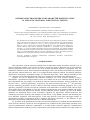
SISOM 2007 and Homagial Session of the Commission of Acoustics, Bucharest 29-31 May
OPTIMIZATION PROCEDURE FOR PARAMETER IDENTIFICATION
IN INELASTIC MATERIAL INDENTATION TESTING
Dan DUMITRIU*, Gaston RAUCHS**, Veturia CHIROIU*
*
**
Institute of Solid Mechanics, Romanian Academy, Bucharest, Romania
Laboratoire de Technologies Industrielles, Centre de Recherche Public Henri Tudor, Grand Duchy of Luxembourg
Corresponding author: D. Dumitriu, Address: Str. Ctin Mille nr. 15, Sector 1, 010141 Bucharest, Romania
Fax: +40 21 3126736, Email: [email protected]
The indentation of an inelastic material isotropic half-space with a spherical tip indenter is simulated
using an in-house finite element code written in Fortran. In order to identify seven unknown material
parameters (E and ν for elasticity; σy,0, R, β, Hkin and Hnl for plasticity), the simulation results must
match as good as possible the experimental load-penetration curve obtained when indenting the
inelastic material. This material parameter identification is performed using an optimization
procedure, i.e., one has to minimize the difference between the experimental curve and the simulated
one. The optimization procedure used here starts by applying a Gauss-Newton method, then continues
using a Levenberg-Marquardt method. Using this optimization procedure, the material parameter
identification was successfully achieved for the considered indentation case study.
Keywords: Indentation, Parameter
Levenberg-Marquardt, convergence.
Identification,
Optimization
Procedure,
Gauss-Newton,
1. INTRODUCTION
This paper deals with the parameter identification in indentation testing of inelastic materials. It is an
inverse engineering problem very relevant to industry, the purpose being to determine one or more inelastic
material parameters that would lead to the most accurate agreement between experimental data and
indentation simulation results. Since indentation modelling involves non-uniform stress fields to be analyzed
and non-linear material behaviour, there is no straight-forward analytical solution for material parameter
identification associated to indentation testing. So, numerical approaches - finite element modelling in this
case - must be used for obtaining the fields of the state variables corresponding to the indentation test.
Suppose one has to determine the unknown parameters of a new inelastic material. Using a
nanoindenter, experimental load-penetration curves are available for the new, unknown material. Based on
this experimental data, the purpose is to identify the unknown material parameters: Young’s modulus E and
Poisson’s ratio ν (elasticity parameters), respectively the initial uniaxial yield stress σ y,0, the non-linear
isotropic hardening parameters R and β and the non-linear kinematic hardening parameters Hkin si Hnl
(plasticity parameters). In what concerns the simulation of the indentation, an in-house FEM code for finite
elasto-plastic strains called SPPRc is used. This software implements the stress update equations and models
the contact between the spherical tip indenter and the unknown inelastic material [1]. The stress update
equations are formulated based on the constitutive equations for hypo-elastic material behaviour and
considering associative plasticity with isotropic J2-flow theory. Using SPPRc software and initializing the
seven unknown parameters with initial guesses in the range between some lower and upper bounds, an
optimization procedure is launched in order to minimize the objective function, i.e., the difference or gap
between the experimental load-penetration curve and the simulated one.
So, by means of the optimization procedure, the material parameters are updated until the minimization
of the objective function is achieved. Several approaches are available for this optimization procedure, from
classical gradient-based numerical optimization to modern neural networks approach. Gradient-based
numerical optimization methods [5] were preferred here, knowing that neural networks need a big amount of
317
Optimization Procedure for Parameter Identification in Inelastic Material Indentation Testing
objective function evaluations and here the computational time for one evaluation is not negligible. Ponthot
and Kleinermann [2] proposed to solve parameter identification inverse problems using a cascade
optimization methodology, i.e., a robust and efficient sequence of gradient-based optimization methods. The
optimization procedure proposed here is a sequence of two gradient-based optimization methods, i.e., the
Gauss-Newton method and the Levenberg-Marquardt method. The gradient of the objective function, i.e., the
vector of the objective function derivatives with respect to the unknown parameters, is computed in a
sensitivity analysis, using the direct differentiation method to calculate the derivatives of the state variables
with respect to the material parameters. This direct differentiation method calculates directly the derivatives,
through an incremental linear update scheme during the incremental solution of the direct deformation
problem [1]. The computational effort is thus considerably reduced, compared with the numerical calculation
of the derivatives by finite differences.
2. THE MATERIAL BEHAVIOUR: CONSTITUTIVE AND STRESS UPDATE EQUATIONS
Associative plasticity with isotropic J2-flow theory is considered [1]. Plastic yielding is governed by
the yield function f :
f = P : (σ − α) − K
⎧ f < 0 for elastic material behavior,
⎪
⎨ f = 0 for plastic material behavior,
⎪ f > 0 excluded,
⎩
y
(1)
where K y is the yield limit, α the back-stress, an internal variable, σ is the Cauchy stress and P is the
deviatoric projection operator
P = IS − 1 I ⊗ I ,
3
(2)
where IS is the fourth-order symmetric identity tensor. The variation of the yield limit K y is described
through isotropic hardening, with [1]:
{
}
K y = 2 σ y ,0 + R [1 − exp(−β s )] ,
3
β
(3)
where s is the plastic arc length, σ y ,0 is the initial uniaxial yield stress, and R and β are the non-linear
isotropic hardening parameters. For kinematic hardening, the Armstrong-Frederick law with the non-linear
kinematic hardening parameters Hkin and Hnl is considered:
α = H kin ε p − 2 H nl s α .
3
(4)
The hypo-elastic material behaviour is described using Hooke’s law, relating the Cauchy stress σ to the
elastic strains ε el through the Lamé constants G and λ:
σ = (2G I S + λ I ⊗ I ) : ε el = C : ε el ,
(5)
where C is the corresponding fourth-order tensor.
Based on the constitutive equations above, the stress update equations can now be formulated. The
state variables at the beginning of an increment are characterized by a superscript ‘0’, whereas those at the
end of the increment are characterized by a superscript ‘1’, and the mid-step configurations are characterized
by a superscript ‘1/ 2’. In the finite strain case, rigid body rotation is accounted for to preserve material
objectivity, henceforth a corotational formulation is used in order to transform all tensor-valued state
variables into the same rotation-neutralized coordinate frame.
In this rotation-neutralized coordinate frame, the classical update scheme of the plastic arc length s, of
the plastic strain ε p , of the stress σ and of the back-stress α is [1]:
Dan DUMITRIU, Gaston RAUCHS, Veturia CHIROIU
s1 = s 0 + 2 Δg ,
3
p,1
p,0
ˆ1,
εˆ = εˆ + ΔgN
318
(6)
(7)
ˆ1,
σˆ 1 = σˆ 0 + C : Δεˆ1 2 − 2GΔgN
αˆ 1 = exp( − H nl Δg ) αˆ 0 + [1 − exp(− H nl Δg )]
(8)
H kin ˆ 1
N ,
H nl
(9)
ˆ
with the total strain increment Δεˆ1 2 calculated according to the midpoint-rule, and the normalized tensor N
defined by:
1
1
ˆ1 1
ˆ1 1
ˆ 1 = P : (σˆ − αˆ ) = P : (σˆ − αˆ ) .
N
y
K
Pˆ 1 : (σˆ 1 − αˆ 1 )
(10)
The plastic consistency parameter Δg is obtained from the equation expressing the yield function (1) for
plastic material behaviour:
f = P : σˆ 0 + 2G P : Δεˆ1 2 − exp(− H nl Δg ) αˆ 0 − 2G Δg −
H kin
[1 − exp(− H nl Δg )] − K y = 0 .
H nl
(11)
A local Newton-Raphson scheme is used to determine Δg from (11).
3. UNIAXIAL INDENTATION TEST
The uniaxial indentation test consists in pushing a hard indenter vertically into the plane surface of the
material specimen (Fig. 1a). A nanoindenter can record the load P and the penetration htip of the indenter tip
into the surface, where the penetration htip is the total displacement of the specimen contact surface at the
vertical line of symmetry. The spherical tip of the indenter has hypo-elastic material behaviour, with
Young’s modulus Etip = 1016 GPa and Poisson’s ratio ν tip = 0.07 .
a)
Fig. 1.: a) Scheme of the uniaxial indentation test, b) Axisymmetric finite element model of the indentation test [1]
319
Optimization Procedure for Parameter Identification in Inelastic Material Indentation Testing
In this inelastic material indentation problem, the parameter identification concerns seven unknown
material parameters: Young’s modulus E and Poisson’s ratio ν (elasticity parameters), respectively the initial
uniaxial yield stress σ y,0, the non-linear isotropic hardening parameters R and β and the non-linear kinematic
hardening parameters Hkin si Hnl (plasticity parameters). In fact, the linear hardening parameters R and Hkin
have been replaced with the following parameters, which both have the physical meaning of a stress:
*
H kin
=
H kin
H nl
and R* =
R
.
β
(12)
The axisymmetric finite element model for spherical indenter tip and material specimen is shown in
Fig. 1b, where 112 bi-quadratic elements were used to model half of the material specimen and 47 biquadratic elements were used to model half of the spherical tip indenter. The simulations are performed
using SPPRc which implements the stress update equations (6)-(9) for this axisymmetric finite element
model, considering finite elasto-plastic strains.
In SPPRc, the contact modelling between the indenter tip and the material specimen is realized by
inhibiting the geometrical interpenetration of the two bodies. This can be achieved by applying tractions over
the contact area. The surface of the indenter is the master surface, whereas the nodes on the material
specimen surface are the slave nodes. In simple contact formulations like penalty or augmented logarithmic
barrier methods, the tractions to be applied on the contact boundary for inhibiting interpenetration are
calculated from the local gap between slave nodes and their projection on the master segment. More details
about the contact modelling can be found in [1].
The indentation test considered here is in fact a virtual indentation test, the purpose being mainly to
validate the proposed material parameter identification optimization procedure. More precisely, a simulation
of the indentation test is carried out with known material parameters, and the resulting load-penetration curve
(see Fig. 2) is used as artificial experimental data, called also pseudo-experimental data. The material
parameters used to obtain the pseudo-experimental data are given in Table 1. The parameter identification
optimization procedure is then started with a different set of material parameters, a virtual initial guess, and
should ideally converge to the material parameters used to obtain the pseudo-experimental data.
Table 1. Material parameters used in the artificial experiment
E [MPa] ν σ y,0 [MPa]
Artificial experiment 200000 0.3
400
R* [MPa] β [-]
100
100
*
[MPa]
H kin
200
Hnl [-]
50
The artificial, pseudo-experimental load-penetration curve considered in this paper concerns only a
single load-unload cycle (see Fig. 2). Of course, more complex cycles can be considered, e.g., load-unloadreload-load-unload cycle, also residual imprint mapping data can be taken into consideration.
8000
7000
load [microN]
6000
5000
4000
3000
2000
1000
0
0
0.05
0.1
0.15
0.2
0.25
penetration into surface [microns]
Fig. 2. Artificial, pseudo-experimental load-penetration curve for single load-unload cycle
Dan DUMITRIU, Gaston RAUCHS, Veturia CHIROIU
320
4. PARAMETER IDENTIFICATION OPTIMIZATION PROCEDURE
Let x denote the vector of the seven material parameters to be identified:
T
*
H nl ⎤⎦ .
x = ⎡⎣ E ν σ y ,0 R* β H kin
(13)
The material parameter identification is performed using an optimization procedure, i.e., one has to
minimize (bring to zero, if possible) the difference between the simulated curve and the pseudo-experimental
one. Both load-penetration curve and residual imprint mapping data are considered for comparing simulation
with pseudo-experimental results. The objective function to be minimized is thus:
Ξ=
N
∑
k =1
with
-
sim
⎡ htip
(Pk ) −
⎣
2
exp
htip
( P k ) ⎤⎦
+
N*
∑{[u
sim
l =1
(r l ) − u sim (r 0 )] − [u exp (r l ) − u exp (r 0 )]} ,
2
(14)
N : the number of points in which simulated and pseudo-experimental penetrations are compared,
sim
htip
( P k ) : the simulated penetration of the indenter tip into the surface corresponding to the load P k
at time t k , using the material parameters computed at that stage of the optimization procedure,
exp
htip
( P k ) : pseudo-experimental penetration corresponding to load P k ;
-
N * : number of fixed radial locations r l where simulated and pseudo-experimental residual imprints
are compared,
u sim (r l ) : the simulated total vertical displacement at the fixed radial location r l ,
-
u sim (r 0 ) : simulated total vertical displacement at the reference point r 0 , e.g., the imprint centre,
-
u exp (r l ) : pseudo-experimental total vertical displacement at the fixed radial location r l ,
-
u exp (r 0 ) : pseudo-experimental total vertical displacement at the reference point r 0 .
-
The gradient of the objective function Ξ with respect to the variables vector x is:
⎡ ∂Ξ
∇Ξ = ⎢
⎣ ∂x1
∂Ξ
∂x2
∂Ξ
∂x3
∂Ξ
∂x4
∂Ξ
∂x5
∂Ξ
∂x6
T
⎡ ∂Ξ
∂Ξ ⎤
⎥ =⎢
∂x7 ⎦
⎣ ∂E
∂Ξ
∂ν
∂Ξ
∂σ y ,0
∂Ξ
∂R*
∂Ξ
∂β
∂Ξ
*
∂H kin
T
∂Ξ ⎤
⎥ ,
∂H nl ⎦
(15)
where the derivative of the objective function Ξ with respect to the material parameter xi (i=1,…,7) follows
from (14):
sim
N
∂htip
(Pk )
∂Ξ
exp
sim
= 2 ⎣⎡ htip
( P k ) − htip
( P k ) ⎦⎤
+
∂xi
∂xi
k =1
∑
N*
∂[u sim (r l ) − u sim (r 0 )]
+ 2 {[u sim (r l ) − u sim (r 0 )] − [u exp (r l ) − u exp (r 0 )]}
.
∂xi
l =1
∑
sim
∂htip
(Pk )
(16)
∂[u sim (r l ) − u sim (r 0 )]
, they are computed from the derivatives of the
∂xi
∂xi
state variables with respect to the material parameter xi . The direct differentiation method is used to perform
this sensitivity analysis as described in [1]. The elements Hij of the Hessian matrix H, i.e., the second order
∂ 2Ξ
, can be deduced by deriving (16):
derivatives
∂xi ∂x j
As for the derivatives
and
321
Optimization Procedure for Parameter Identification in Inelastic Material Indentation Testing
H ij =
sim
N ⎧ ∂hsim ( P k ) ∂hsim ( P k )
∂ 2 htip
( P k ) ⎫⎪
∂ 2Ξ
⎪ tip
tip
exp
sim
=2 ⎨
+ ⎣⎡ htip
( P k ) − htip
( P k ) ⎦⎤
⎬+
∂xi ∂x j
∂x j
∂xi ∂x j ⎭⎪
⎪ ∂xi
k =1 ⎩
∑
+2
⎧⎪ ∂[u sim (r l ) − u sim (r 0 )] ∂[u sim (r l ) − u sim (r 0 )]
+
∂xi
∂x j
l =1 ⎩
N*
∑ ⎨⎪
+ ⎡⎣(u sim (r l ) − u sim (r 0 )) − (u exp (r l ) − u exp (r 0 )) ⎤⎦
(17)
∂ 2 [u sim (r l ) − u sim (r 0 )] ⎫⎪
⎬.
∂xi ∂x j
⎪⎭
The optimization procedure proposed in this paper is a sequence of two gradient-based optimization
methods, i.e., the Gauss-Newton method and the Levenberg-Marquardt method. The optimization problem
here is a minimization with simple bounds, i.e., the variables of the minimization problem are limited by
constant lower and upper bounds.
The Gauss-Newton optimization method is an iterative method based on the following recurrence
relation [4]-[5]:
x p +1 = x p − μ p [H p ]−1 (∇Ξ) p ,
(18)
where p denotes here the iteration number and μ p is the parameter of the line search algorithm performed
inside the Gauss-Newton method to find the lowest value of the objective function Ξ along the search
direction [H p ]−1 (∇Ξ) p . The Hessian matrix H p given by (17) has to be positive definite in order to provide
that the search direction is a descent direction [3], i.e, in order to converge towards a minimum of the
objective function.
As for the Levenberg-Marquardt optimization method [3]-[5], its recurrence relation is:
x p +1 = x p − [( J p ) T J p + ξ p I ]−1 ( J p )T Ξ p ,
(19)
where J is the Jacobian defined here as
⎡ ∂Ξ
J=⎢
⎣ ∂E
∂Ξ
∂ν
∂Ξ
∂σ y ,0
∂Ξ
∂R*
∂Ξ
∂β
∂Ξ
*
∂H kin
∂Ξ ⎤
T
⎥ = ( ∇Ξ ) ,
∂H nl ⎦
(20)
and where the scalar ξ p is determined as follows:
ξ p = 10 −15
DO ξ p = 10 ⋅ ξ p
UNTIL matrix [( J p )T J p + ξ p I ] becomes positive definite
(21)
The implementation in SPPRc software of the Gauss-Newton and Levenberg-Marquardt methods was
done by means of the respective subroutines provided by IMSL Fortran Math Library [4].
5. CONVERGENCE RESULTS
The parameter identification optimization procedure proposed in §4 was applied to the virtual uniaxial
indentation problem described in §3. The pseudo-experimental load-penetration curve is the one shown
previously in Fig. 2, where only a single load-unload cycle has been considered. The residual imprint
mapping data taken into account in provided in Table 2, with the reference point located on the vertical
symmetry axis, i.e., r 0 = 0 .
Dan DUMITRIU, Gaston RAUCHS, Veturia CHIROIU
322
Table 2. Residual imprint mapping data
index l
1
2
3
4
5
6
7
8
9
l
0.125 0.250 0.375 0.500 0.625 0.750 0.875 1.000 1.125
r [μm]
exp
l
exp
0
u (r ) − u (r ) [μm] 0.0035 0.0127 0.0279 0.0495 0.0775 0.1121 0.1536 0.2019 0.2462
10
11
12
13
14
15
16
17
18
19
20
1.250 1.375 1.500 1.625 1.750 1.875 2.000 2.125 2.250 2.375 2.500
0.2383 0.2314 0.2265 0.2231 0.2205 0.2185 0.2168 0.2156 0.2146 0.2138 0.2132
Starting from various virtual initial guesses, the optimization procedure proposed in §4 is supposed to
converge to the material parameters used to obtain the pseudo-experimental data, i.e., the ones in Table 1.
Two such convergence tests T1 and T2 were performed, Table 3 presenting the virtual initial guesses used in
these two tests, as well as the lower and upper bounds of the seven parameters to be identified, plus the
solution of the problem, i.e., the pseudo-experimental material parameters from Table 1.
Table 3. Different values for the material parameters : T1 and T2 initial guesses, upper and lower bounds, problem’s solution
E [MPa]
T1 initial guesses
100000
T2 initial guesses
261110
Artificial experiment 200000
Lower bounds
30000
Upper bounds
600000
σ y,0 [MPa]
ν
0.2
800
0.34
667
0.3
400
0.05
1
0.49
1000
β [-]
R* [MPa]
50
200
46
523
100
100
0
10
1000
1500
*
[MPa]
H kin
50
398
200
0
1000
Hnl [-]
100
74
50
10
1500
The proposed optimization procedure consists in a sequence of fours stages:
• Gauss-Newton method (18) applied on variables E and σ y,0, the other variables being blocked on
their initial guesses (called G-N1, maximum 8 iterations allowed);
• Gauss-Newton method (18) applied on all seven variables (called G-N2, maximum 10 iterations);
• Levenberg-Marquardt method (19) applied on three variables (the variables located temporarily on
∂Ξ
), the other four variables being
the bounds, then the variables xi corresponding to the smallest
∂xi
blocked on their previous values (called L-M1, maximum 15 iterations allowed);
• Levenberg-Marquardt method (19) applied on all seven variables (called L-M2, maximum 30
iterations allowed).
Fig. 3a shows the convergence of the optimization procedure for the first numerical test T1, where the
objective function is minimized up to Ξ min,T1 = 1.28 ⋅10-12 [μm2]. Fig. 3b shows the convergence results for
the second numerical test T2, where the objective function is minimized up to Ξ min,T2 = 7.16 ⋅ 10-9 [μm2].
Both figures show the reduction of log10 Ξ with the number of iterations performed. The vertical dotted lines
indicate the switches between the four stages of the optimization procedure.
The results are satisfactory, showing the reliability of the proposed four stages optimization procedure,
based on Gauss-Newton and Levenberg-Marquardt methods. The objective function is always decreasing for
both tests presented, without diverging or blocking in undesired local minima. The objective function has
been practically brought to zero, the material parameters obtained by this identification procedure matching
almost perfectly the considered pseudo-experimental material parameters.
323
Optimization Procedure for Parameter Identification in Inelastic Material Indentation Testing
Fig. 3. Reduction of log10 Ξ with the number of iterations, for: a) first test T1; b) second test T2.
6. CONCLUSIONS
The framework of this work is the parameter identification related to inelastic material indentation
testing. The goal of this inverse problem is to determine the unknown material parameters of a specimen, in
order to reach some experimental data measured on that specimen.
More precisely, the purpose of this paper was to propose a reliable variant of optimization procedure
for this material parameter identification problem. Based on IMSL Fortran Math Library [4] subroutines, the
optimization procedure was implemented in SPPRc, an in-house FEM software for finite elasto-plastic
strains. The optimization procedure was divided in four stages, two stages based on Gauss-Newton method,
followed by two stages based on Levenberg-Marquardt method. The convergence results towards the desired
global minimum were satisfactory. Further investigations, including additional load cycles of the indentation
test, are necessary in order to increase and guarantee the reliability of this parameter identification
optimization procedure.
Gradient-based optimization methods, such as Gauss-Newton and Levenberg-Marquardt methods, are
local optimizers, bearing the necessity to supply an appropriate initial guess, in order to place the
optimization problem closer to its searched global optimum. So, further work may provide a more elaborated
initialization of the unknown material parameters, not just a simple guess.
ACKNOWLEDGEMENTS. Gaston RAUCHS gratefully acknowledges the financial support of the Fonds
National de la Recherche (FNR) of the Grand Duchy of Luxembourg, through grant number FNR-05/02/01VEIANEN.
Dan DUMITRIU and Veturia CHIROIU gratefully acknowledge the financial support of the National
Authority for Scientific Research Council (ANCS), Romania, through CEEX postdoctoral grant nr.
1531/2006, which funded the visit of Dan DUMITRIU at the Centre de Recherche Public Henri Tudor.
REFERENCES
1. RAUCHS, G., Optimization-based material parameter identification in indentation testing for finite strain elasto-plasticity,
ZAMM - Z. Angew. Math. Mech., 86, 7, pp. 539–562, 2006.
2. PONTHOT, J.-P., KLEINERMANN, J.-P., A cascade optimization methodology for automatic parameter identification and
shape/process optimization in metal forming simulation, Comput. Methods Appl. Mech. Engrg., 195, pp. 5472–5508, 2006.
3. SEIFERT, T., SCHENK, T., SCHMIDT, I., Efficient and modular algorithms in modeling finite inelastic deformations: Objective
integration, parameter identification and sub-stepping techniques, Comput. Methods Appl. Mech. Engrg., 196, pp. 2269–
2283, 2007.
4. IMSL Math/Library vol. 1 and 2 - FORTRAN Subroutines for Mathematical Applications, Visual Numerics, Inc., pp. 867–1029
(Chapter 8: Optimization), 1997.
5. NOCEDAL, J., WRIGHT, S.J., Numerical Optimization, Springer Verlag, New York, 1999.