1
Metanet User’s Guide and Tutorial
Claude Gomez
Maurice Goursat
Manual version 1.1 for Scilab 2.4
Metanet is a toolbox of Scilab for graphs and networks computations. It comes as new Scilab functions together with a graphical window for displaying and modifying graphs.
You can use the Metanet toolbox in Scilab without using the graphical window window at all, i.e.
without seeing the graphs or the networks you are working with.
1 Representation of graphs
The graphs handled by Metanet are directed or undirected multigraphs (loops are allowed). A graph is a
set of arcs and nodes.
A graph must have at least one arc. We call arc a directed link between two nodes. For instance
the arc (i; j ) goes from tail node i to head node j . We call edge the corresponding undirected link. A
minimal way to represent a graph is to give the number of nodes, the list of the tail nodes and the list
of the head nodes. Each node has a number and each arc has a number. The numbers of nodes are
consecutive and the number of arcs are consecutive. In Scilab, these lists are represented by row vectors.
So, if we call tail and head these row vectors, the arc number i goes from node number tail(i) to
node number head(i). Moreover, it is necessary to give the number of nodes, because isolated nodes
(without any arc) can exist. The size of the vectors tail and head is the number of edges of the graph.
This is the standard representation of graphs in Metanet as it is described in the graph list (see 1.1). There
are functions to compute other representations better suited for some algorithms (see 1.2).
The distinction between edges and arcs is meaningful when we deal with undirected graphs. This
distinction is not needed when we only use the standard functions of Metanet. There is no distinction
between an arc and a directed edge. We will often use indistinctly these two terms.
A new object, the graph list data structure, is defined in Scilab to handle graph. It is described below.
1.1 The graph list data structure
Metanet uses the graph list data structure to represent graphs. With this type of description (see 1.2), we
can have directed or undirected multigraphs and multiple loops are allowed. The graph list data structure
is a typed list. As usual, the first element of this object is itself a list which defines its type, ’graph’,
and all the access functions to the other elements. The graph list has 33 elements (not counting the first
one defining the type). Only the first five elements must have a value in the list, all the others can be
given the empty vector [] as a value, and then a default is used. These five required elements are:
name name of the graph (a string)
directed flag equal to 1 if the graph is directed or equal to 0 if the graph is undirected
node number number of nodes
1
tail row vector of the tail node numbers
head row vector of the head node numbers
A graph must at least have one arc, so tail and head cannot be empty.
For instance, you can define a graph list (see 2.1) by
g=make_graph(’min’,1,1,[1],[1]);
which is the simplest graph you can create (it is directed, has one node and one loop arc on this node).
Each element of the list can be accessed by using its name. For instance, if g is a graph list and you
want to get the node number element, you only have to type:
g(’node number’)
and if you want to change this value to 10, you only have to type:
g(’node number’)=10
The check graph function checks a graph list to see if there are inconsistencies in its elements.
Checking is not only syntactic (number of elements of the list, compatible sizes of the vectors), but also
semantic in the sense that check graph checks that node number, tail and head elements of
the list can really represent a graph. This checking is automatically made when calling functions with a
graph list as an argument.
You will find below the description of all the elements of a graph list. Each element is described by
one or more lines. The first lines give the name of the element and its definition, with its Scilab type if
needed. The last line gives the default for elements that can have one. The name of the element is used
to access the elements of the list.
name Name of the graph; a string with a maximum of 80 characters (REQUIRED).
directed Flag giving the type of the graph; it is equal to 1 if the graph is directed or equal to 0 is the
graph is undirected (REQUIRED).
node number Number of nodes (REQUIRED).
tail Row vector of the tail node numbers (REQUIRED).
head Row vector of the head node numbers (REQUIRED).
node name Row vector of the node names; they MUST be different.
Default is the node numbers as node names.
node type Row vector of the node types; the type is an integer from 0 to 2:
0: plain node
1: sink node
2: source node
This element is mainly used to draw the nodes in the Metanet window. A plain node is drawn as a
circle. A sink or source node is a node where extraneous flow goes out the node or goes into the
node; it is drawn differently (a circle with an outgoing or ingoing arrow).
Default is 0 (plain node).
node x Row vector of the x coordinates of the nodes.
Default is computed when showing the graph in the Metanet window (see 3).
2
node y Row vector of the y coordinates of the nodes.
Default is computed when showing the graph in the Metanet window (see 3).
node color Row vector of the node colors; the color is an integer from 0 to 16:
0: black
1: navyblue
2: blue
3: skyblue
4: aquamarine
5: forestgreen
6: green
7: lightcyan
8: cyan
9: orange
10: red
11: magenta
12: violet
13: yellow
14: gold
15: beige
16: white
Default is 0 (black).
node diam Row vector of the sizes of the node diameters in pixels (a node is drawn as a circle).
Default is the value of element default node diam.
node border Row vector of the sizes of the node borders in pixels.
Default is the value of element default node border.
node font size Row vector of the sizes of the font used to draw the name or the label of the node; you
can choose 8, 10, 12, 14, 18 or 24.
Default is the value of element default font size.
node demand Row vector of the node demands.
The demands of the nodes are used in functions min lcost cflow, min lcost flow1, min lcost flow2,
min qcost flow and supernode.
Default is 0.
edge name Row vector of the edge names; edge names need not be different.
Default is the edge numbers as edge names.
edge color Row vector of the edge colors; the color is an integer from 0 to 16 (see node color).
Default is 0 (black).
3
edge width Row vector of the sizes of the edge widths in pixels.
Default is the value of element default edge width.
edge hi width Row vector of the sizes of the highlighted edge widths in pixels.
Default is the value of element default edge hi width.
edge font size Row vector of the sizes of the font used to draw the name or the label of the edge; you
can choose 8, 10, 12, 14, 18 or 24.
Default is the value of element default font size.
edge length Row vector of the edge lengths.
The lengths of the edges are used in functions graph center, graph diameter, salesman
and shortest path.
Default is 0.
edge cost Row vector of the edge costs.
The costs of the edges are used in functions min lcost cflow, min lcost flow1 and min lcost flow2.
Default is 0.
edge min cap Row vector of the edge minimum capacities.
The minimum capacities of the edges are used in functions max flow, min lcost cflow,
min lcost flow1, min lcost flow2 and min qcost flow.
Default is 0.
edge max cap Row vector of the edge maximum capacities.
The maximum capacities of the edges are used in functions max cap path, max flow, min lcost cflow,
min lcost flow1, min lcost flow2 and min qcost flow.
Default is 0.
edge q weight Row vector of the edge quadratic weights. It corresponds to
cost on edge u with flow '(u): 12 w(u)('(u) w0 (u))2 .
w(u) in the value of the
The quadratic weights of the edges are used in function min qcost flow.
Default is 0.
edge q orig Row vector of the edge quadratic origins. It corresponds to w0 (u) in the value of the cost
on edge u with flow '(u): 12 w(u)('(u) w0 (u))2 .
The quadratic origins of the edges are used in function min qcost flow.
Default is 0.
edge weight Row vector of the edge weights.
The weights of the edges are used in function min weight tree.
Default is 0.
default node diam Default size in pixels of the node diameters of the graph.
Default is 20.
4
default node border Default size in pixels of the node borders of the graph.
Default is 2.
default edge width Default size in pixels of the edge widths of the graph.
Default is 1.
default edge hi width Default size in pixels of the highlighted edge widths of the graph.
Default is 3.
default font size Default size of the font used to draw the names or the labels of nodes and edges.
Default is 12.
node label Row vector of the node labels.
Node labels are used to draw a string in a node. It can be any string. An empty label can be given
as a blank string ’ ’.
edge label Row vector of the edge labels.
Edge labels are used to draw a string on an edge. It can be any string. An empty label can be given
as a blank string ’ ’.
1.2 Various representations of graphs
1.2.1
Names and numbers
First of all, we need to distinguish between the name of a node or the name of an edge and their internal
numbers. The name can be any string. Its is saved in the graph file (see 2.2). The internal number
is generated automatically when loading a graph. The nodes and the edges have consecutive internal
numbers starting from 1. When using the Scilab functions working on graphs, all the computations are
made with internal numbers.
It is very important to give different names to the nodes because the nodes are distinguished by their
names when they are loaded. This distinction is not important for edges.
Often, the names are taken as the internal numbers. This is the default when no names are given. In
this case, the distinction between a name and a number is not meaningful. Only the type of the variable
is not the same: the name is a string and the number is an integer.
In the following when we talk about the number of a node or the number of an edge, we mean the
internal number.
1.2.2
Tail head
We have seen that the standard representation of a graph used by Metanet is by the means of two row
vectors tail and head: arc number i goes from node number tail(i) to node number head(i).
The size of these vectors is the same and is the number of arcs of the graph.
Moreover the number of nodes must be given. It is greater than or equal to the maximum integer
number in tail and head. If node numbers do not belong to tail and head then there are isolated
nodes.
If the graph is undirected, it is the same, but tail(i) and head(i) can be exchanged.
This representation is very general and gives directed or undirected multigraphs with possible loops
and isolated nodes.
5
4
2
1
3
3
4
1
2
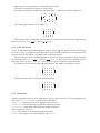
Figure 1: Small directed graph
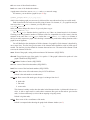
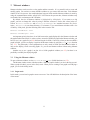
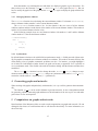
The standard function to create graphs is make graph (see 2.1). For instance, we can create a small
directed graph with a loop and an isolated node (see figure 1) by using:
node number = 4, tail = [1,1,2,3], head = [2,3,1,3],
or in Scilab:
g=make graph(’foo’,1,4,[1 1 2 3],[2 3 1 3]);
1.2.3
Adjacency lists
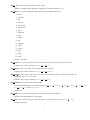
Another interesting representation often used by algorithms is the adjacency lists representation. It uses
three row vectors, lp, ls and la. If n is the number of nodes and m is the number of arcs of the graph:
lp is the pointer array (size = n + 1)
ls is the node array (size = m)
la is the arc array (size = m).
If the graph is undirected, each edge corresponds to two arcs.
With this type of representation, it is easy to know the successors of a node. Node number i has
lp(i+1)-lp(i) successors nodes with numbers from ls(lp(i)) to ls(lp(i+1)-1), the corresponding arcs are have numbers from la(lp(i)) to la(lp(i+1)-1).
The adjacency lists representation of the graph of figure 1 is given below:
1
2
3
4
5
lp
1
3
4
5
5
ls
2
3
1
3
la
1
2
3
4
The function used to compute the adjacency list representation of a graph is adj lists.
1.2.4
Node-arc matrix
For a directed graph, if n is the number of nodes and m is the number of arcs of the graph, the node-arc
matrix A is a n m matrix:
if A(i; j ) = +1, then node i is the tail of arc j
if A(i; j ) = 1, then node i is the head of arc i.
If the graph is undirected and m is the number of edges, the node-arc matrix A is also a n m matrix
and:
if A(i; j ) = 1, then node i is an end of edge j .
6
With this type of representation, it is impossible to have loops.
This matrix is represented in Scilab as a sparse matrix.
For instance, the node-arc matrix corresponding to figure 1, with loop arc number 4 deleted is :
0
B
B
B
@
1
1
1
0
0
1
0
0
If the same graph is undirected, the matrix is:
0
BB 11
B@ 0
0
1
C
1 C
C
0 A
1
1
0
1
0
1
C
1 C
C
0 A
1
0
0
The functions used to compute the node-arc matrix of a graph, and to come back to a graph from the
node-arc matrix are graph 2 mat and mat 2 graph.
1.2.5
Node-node matrix
The n n node-node matrix of the graph is the matrix A where A(i; j ) = 1 if there is one arc from node
i to node j . Only 1 to 1 graphs (no more than one arc from one node to another) can be represented, but
loops are allowed. This matrix is also known as the “adjacency matrix”.
The same functions used to compute the node-arc matrix (see above) of a graph are used to compute
the node-node matrix: graph 2 mat and mat 2 graph. To specify that we are working with the
node-node matrix, the flag ’nodenode’ must be given as the last argument of these functions.
For instance, you can find below the node-node matrix of the graph corresponding to Figure 1:
0
BB 01
B@ 0
0
1
1
0
0
0
1
0
0
1
C
0 C
C
0 A
0
0
and the node-node matrix for the same undirected graph:
0
BB 01
B@ 1
0
1.2.6
1
1
0
0
0
1
0
0
1
C
0 C
C
0 A
0
0
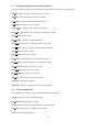
Chained lists
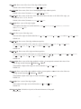
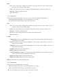
Another representation used by some algorithms is given by the chained lists. This representation uses
four vectors, fe, che, fn and chn which are described below:
e1=fe(i)) is the number of the first edge starting from node i
e2=che(e1) is the number of the second edge starting from node i
e3=che(e2) is the number of the third edge starting from node i
and so on until the value is 0
fn(i) is the number of the first node reached from node i
chn(i) is the number of the node reached by edge che(i).
7
00000000000
11111111111
00000000000000000000
11111111111111111111
11111111111
00000000000
00000000000
11111111111
00000000000000000000
11111111111111111111
00000000000 1010 11111111111
11111111111
00000000000
00000000000000000000
11111111111111111111
00000000000
11111111111
00000000000
11111111111
00000000000000000000
11111111111111111111
1010 11111111111
00000000000
11111111111
00000000000
00000000000000000000
11111111111111111111
00000000000 11111111111
11111111111
00000000000
00000000000000000000101100 10
11111111111111111111
101100 10
i
e1=fe(i)
e2=che(e1)
fn(i)
e3=che(e2)
chn(e1)
chn(e2)
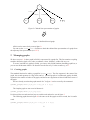
Figure 2: Chained lists representation of graphs
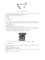
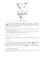
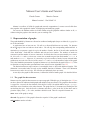
1
1
Figure 3: Smallest directed graph
All this can be more clearly seen on figure 2.
You can use the chain struct function to obtain the chained lists representation of a graph from
the adjacency lists representation (see 1.2.3).
2 Managing graphs
We have seen (see 1.1) that a graph in Scilab is represented by a graph list. This list contains everything
needed to define the graph, arcs, nodes, coordinates, colors, attributes, width of the arcs, etc.
To create, load and save graphs in Scilab, you can use only Scilab functions, handling graph lists, or
you can use the Metanet window. We describe here the first way. For the second way, see 3.
2.1 Creating graphs
The standard function for making a graph list is make graph. The first argument is the name of the
graph, the second argument is a flag which can be 1 (directed graph) or 0 (undirected graph), the third
argument is the number of nodes of the graph, and the last two arguments are the tail and head vectors of
the graph.
We have already seen that the graph named “foo” in figure 1 can be created by the command:
g=make_graph(’foo’,1,4,[1 1 2 3],[2 3 1 3]);
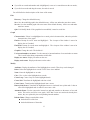
The simplest graph we can create in Metanet is:
g=make_graph(’min’,1,1,[1],[1]);
It is directed, has one node and one loop arc on this node and can be seen in figure 3.
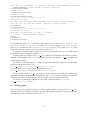
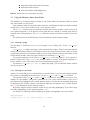
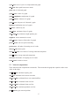
The following graph shown in figure 4 is the same as the first graph we have created, but it is undirected:
g=make_graph(’ufoo’,0,4,[1 1 2 3],[2 3 1 3]);
8
4
2
1
3
3
4
1
2
Figure 4: Small undirected graph
3
1
1
2
4
4
3
Figure 5: Directed graph
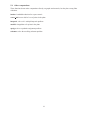
You can also give 0 as the third argument of make graph (number of nodes). This means that
make graph will compute itself from its last arguments, the tail and head vectors, the number of nodes
of the graph. So, this graph has no isolated node and the nodes names are taken from the numbers in tail
and head vectors. For instance, if you enter
g=make_graph(’foo1’,1,0,[1 1 4 3],[4 3 1 3]);
the graph (shown in figure 5) has three nodes with names 1, 3 and 4, no isolated node and four edges.
Note the difference with the graph of figure 1.
The other elements of the graph list (see 1.1) can be entered by using the names of the elements. For
instance, to give graph “foo” coordinates for the nodes, you can enter:
g=make_graph(’foo’,1,4,[1 1 2 3],[2 3 1 3]);
g(’node_x’)=[42 108 176 162];
g(’node_y’)=[36 134 36 93];
Another simple example: if you want to transform the directed graph g into an undirected graph, you
only have to do:
g(’directed’)=0;
There is a wizard way to create a graph list “by hands” without using the make graph function.
This can be useful when writing your own Scilab functions. You can use the Scilab function glist
which must have as many arguments as the elements of the graph list (see 1.1). This way can lead to
errors, because the list is somehow long. You can use the check graph function to check if the graph
list is correct.
2.2 Loading and saving graphs
Graphs are saved in ASCII files, called graph files. A graph file has the extension .graph. The structure
of a graph file is given below:
9
GRAPH TYPE (0 = UNDIRECTED, 1 = DIRECTED), DEFAULTS (NODE DIAMETER, NODE BORDER,
first line continuing ARC WIDTH, HILITED ARC WIDTH, FONTSIZE):
<one line with above values>
NUMBER OF ARCS:
<one line with the number of arcs>
NUMBER OF NODES:
<one line with the number of nodes>
****************************************
DESCRIPTION OF ARCS:
ARC NAME, TAIL NODE NAME, HEAD NODE NAME, COLOR, WIDTH, HIWIDTH, FONTSIZE
COST, MIN CAP, CAP, MAX CAP, LENGTH, Q WEIGHT, Q ORIGIN, WEIGHT
<one blank line>
<two lines for each arc>
****************************************
DESCRIPTION OF NODES:
NODE NAME, POSSIBLE TYPE (1 = SINK, 2 = SOURCE)
X, Y, COLOR, DIAMETER, BORDER, FONTSIZE
DEMAND
<one blank line>
<three lines for each node>
For an undirected graph, ARC is replaced by EDGE. Moreover, the values of NODE DIAMETER, NODE
BORDER, ARC WIDTH, HILITED ARC WIDTH and FONTSIZE for the graph, COLOR, WIDTH, HIWIDTH
and FONTSIZE for the arcs, and POSSIBLE TYPE, COLOR, DIAMETER, BORDER and FONTSIZE for the
nodes can be omitted or equal to 0, then the default is used (see 1.1).
It is possible to create by hands a graph file and to load it into Scilab, but it is a very cumbersome
job. Programs are given to generate graphs (see 4).
To load a graph into Scilab, use the load graph function. Its argument is the absolute or relative
pathname of the graph file; if the .graph extension is missing, it is assumed. load graph returns the
corresponding graph list.
For instance, to load the graph foo, which is in the current directory, and put the corresponding
graph list in the Scilab variable g, do:
g=load graph(’foo’); or g=load graph(’foo.graph’);.
To load the graph mesh100 given in the Scilab distribution, do:
g=load graph(SCI+’/demos/metanet/mesh100.graph’);
To save a graph, use the save graph function. Its first argument is the graph list, and its second
argument is the name or the pathname of the graph file; if the .graph extension is missing, it is assumed.
If the path is the name of a directory, the name of the graph is used as the name of the file.
For instance, the following command saves the graph g into the graph file foo.graph:
save graph(g,’foo.graph’);
2.3 Plotting graphs
The fastest way to see a graph is to plot it in a Scilab graphical window. We can use the plot graph
function to do this. Note that no interaction is possible with the displayed graph. If you want to graphically modify the graph, use Metanet windows (see 3).
10
3 Metanet windows
Metanet windows can be used to see the graphs and the networks. It is a powerful tool to create and
modify graphs. You can have as many Metanet windows as you want at the same time. Each Metanet
window is an Unix process: the communications between Scilab and the Metanet windows is made by
using the communication toolbox called GeCI. NOTE that at the present time, Metanet windows only
work under Unix environment with X Window.
By default, the size of Metanet windows is 1000 pixels by 1000 pixels. If you want to see big
graphs, you have to change this values by using X Window ressources. Put the new values in the ressources Metanet.drawWidth and Metanet.drawHeight in a standard ressource file (for instance .Xdefaults in your home directory). For instance, if you want Metanet windows with a size
of 2000 by 3000 pixels, puts the following lines in the ressource file:
Metanet.drawWidth: 2000
Metanet.drawHeight: 3000
An important point is that there is no link between the graph displayed in the Metanet window and
the graphs loaded into Scilab. So, when you have created or modified a graph in the Metanet window, you
have to save it as a graph file (see 2.2) and load it again in Scilab. Conversely, when you have modified a
graph in Scilab, you have to display it again in the Metanet window by using the save graph function
(see 3.2). The philosophy is that computations are only made in Scilab and the Metanet window is
only used to display, create or modify graphs. So, you can use Metanet toolbox without using Metanet
windows.
Another way to see a graph is to plot it in a Scilab graphical window (see 2.3), but there is no
possibility to modify the displayed graph.
3.1 Using the Metanet window
To open a Metanet window, use the metanet or show graph Scilab functions (see 3.2).
The Metanet window comes with three modes. When no graph is loaded, you are in the Begin mode.
When a graph is loaded, you are in the Study mode. When you are creating a new graph or modifying a
graph, you are in the Modify mode.
3.1.1
Begin mode
In this mode, you can load a graph or create a new one. You will find below the description of the items
of the menus.
11
Files
New Create a new graph. Prompt for the name of the graph and for its type (directed or not
directed). Then you enter Modify Mode.
Load Load a graph. Show the list of graphs in the default directory. You have to choose one.
Directory Change the default directory.
Quit Quit Metanet.
3.1.2
Study mode
In this mode, you can load a graph, create a new one or work with an already loaded graph.
With the left button of the mouse, you can highlight an arc or a node.
You will find below the description of the items of the menus.
Files
New Create a new graph. Prompt for the name of the graph and for its type (directed or not
directed). Then you enter Modify Mode.
Load Load a graph. Show the list of graphs in the default directory. You have to choose one.
Directory Change the default directory.
Save As Save the loaded graph with a new name in the default directory.
Quit Quit Metanet.
Graph
Characteristics If there is an highlighted arc or node, print its characteristics, otherwise print the
characteristics of the graph.
Find Arc Prompt for an arc name and highlight it. The viewport of the window is moved to
display the arc if needed.
Find Node Prompt for a node name and highlight it. The viewport of the window is moved to
display the arc if needed.
Graphics Change the scale. The default is 1.
Modify Graph Enter Modify mode.
Use internal numbers as names Use the consecutive internal numbers of arcs and nodes as names.
This is useful when doing computations with Scilab.
Display arc names Display arc names on the arcs.
Display node names Display node names on the nodes.
Redraw Refresh the screen and redraw the graph.
3.1.3
Modify mode
In this mode, you can modify and save the graph.
With the left button of the mouse, you can highlight an arc or a node.
With the right button of the mouse, you can modify the graph:
if you click where there is no arc or node, a new node is created;
12
if you click on a node and another node is highlighted, a new arc is created between the two nodes;
if you click on a node and drag the mouse, the node is moved.
You will find below the description of the items of the menus.
Files
Directory Change the default directory.
Save Save the modified graph in the default directory. All the arcs and nodes must have names.
Save As Save the modified graph with a new name in the default directory. All the arcs and nodes
must have names.
Quit Exit Modify Mode. If the graph has been modified, it must be saved first.
Graph
Characteristics If there is an highlighted arc or node, print its characteristics, otherwise print the
characteristics of the graph.
Find Arc Prompt for an arc name and highlight it. The viewport of the window is moved to
display the arc if needed.
Find Node Prompt for a node name and highlight it. The viewport of the window is moved to
display the arc if needed.
Graphics Change the scale. The default is 1.
Use internal numbers as names Use the consecutive internal numbers of arcs and nodes as names.
This is useful when doing computations with Scilab.
Display arc names Display arc names on the arcs.
Display node names Display node names on the nodes.
Modify
Attributes Display the attributes of the highlighted arc or node. Then, they can be changed.
Delete Delete the highlighted arc or node. NOTE: there is no undelete.
Name Name the highlighted arc or node.
Color Give a color to the highlighted arc or node.
Create Loop Create a loop arc on the highlighted node.
Create Sink Transform the highlighted node into a sink.
Create Source Transform the highlighted node into a source.
Remove Sink/Source Transform the highlighted source or sink node into a plain node. It has no
effect if the highlighted node is neither a source nor a sink.
Automatic Name Give the consecutive internal arc and node numbers as the names of arcs and
nodes. This can be useful for a new graph. NOTE that if some arcs and nodes already have
names, they are replaced by the corresponding internal numbers.
Default Values Change some default values:
the default size of the font
the default diameter of the nodes
13
the default width of the border of the nodes
the default width of the arcs
the default width of the highlighted arcs
Redraw Refresh the screen and redraw the graph.
3.2 Using the Metanet window from Scilab
The standard way of using the Metanet window is from Scilab. Indeed, the Metanet window is opened
only when needed as a new process.
Many Metanet windows can be opened at the same time. Each Metanet window has a number (integer
starting from 1). One of these windows is the current Metanet window.
The metanet function opens a new Metanet window and returns its number. A path can be given
as an optional argument: it is the directory where graph files are searched; by default, graph files are
searched in the working directory. The metanet function is mainly used when we want to create a new
graph.
We describe below the Scilab functions used in conjunction with the Metanet window.
3.2.1
Showing a graph
The first thing we would like to do is to see the graph we are working with: use the show graph
function.
show graph(g) displays the graph g in the current Metanet window. If there is no current Metanet
window, a new Metanet window is created and it becomes the current Metanet window. If there is already
a graph displayed in the current Metanet window, the new graph is displayed instead. The number of the
current Metanet window, where the graph is displayed, is returned by show graph.
Two optional arguments can be given to show graph(g) after the graph list. If an optional argument is equal to the string ’new’, a new Metanet window is created. If an optional argument is a
positive number, it is the value of the scale factor when drawing the graph (see 3.1).
For instance show graph(g,’new’,2) displays the graph g in a new Metanet window with the
scale factor equal to 2.
3.2.2
Showing arcs and nodes
Another very useful thing to do is to distinguish a set of nodes and/or a set of arcs in the displayed graph.
This is done by highlighting nodes and/or arcs: use the show arcs and show nodes functions.
The arguments of the show arcs and show nodes functions are respectively a row vector of arc
numbers (or edge numbers if the graph is undirected) or a row vector of node numbers. These sets of
arcs and nodes are highlighted in the current Metanet window. Note that the corresponding graph must
be displayed in this window, otherwise the numbers might not correspond to arcs or nodes numbers
(see 3.2.3 for changing the current Metanet window).
By default, using one of these functions switch off any preceeding highlighting. If you want to keep
preceeding highlighting, use the optional argument ’sup’.
For instance, the following commands displays the graph g and highlights 3 arcs and 2 nodes:
show_graph(g)
show_arcs([1 10 3]); show_nodes([2 7],’sup’)
14
Note that another way to distinguish arcs and nodes in a displayed graph is to give them colors. For
that you have to use the elements edge color and node color of the graph list (see 1.1). But you
have to modify the graph list of the graph and use show graph again to display the graph with the new
colors.
3.2.3
Managing Metanet windows
The netwindow function is used to change the current Metanet window. For instance netwindow(2)
chooses Metanet window number 2 as the current Metanet window.
The netwindows function returns a list. Its first element is the row vector of all the Metanet
windows numbers and the second element is the number of the current Metanet window. This number is
equal to 0 if no current Metanet window exists.
In the following example, there are two Metanet windows with numbers 1 and 3 and the Metanet
window number 3 is the current Metanet window.
-->netwindows()
ans =
ans(1)
!
1.
3. !
ans(2)
3.
3.2.4
Synchronism
By default Metanet windows work with Scilab in asynchronous mode, i.e. Scilab proceeds without waiting for graphics commands sent to Metanet windows to terminate. This mode is the most efficient. But
when running a lots of graphics commands, problems can arise. For instance, you might highlight a
set of nodes in a bad Metanet window because the good one has not yet appeared! So it is possible to
use a synchronous mode. Then Scilab waits until the functions dealing with the Metanet windows have
terminated.
The metanet sync function is used to change the mode: metanet sync(0) changes to asynchronous mode (default), metanet sync(1) changes to synchronous mode, and metanet sync()
returns the current mode (0 = asynchronous, 1 = synchronous).
4 Generating graphs and networks
When working with graphs and particularly with networks, it is very useful to generate them automatically.
The function gen net can be used in Metanet to generate networks. It uses a triangulation method
for generating a planar connected graph and then uses the information of the user to give arcs and nodes
good values of costs and capacities.
5 Computations on graphs and networks
Most functions of the Metanet toolbox are used to make computations on graphs and networks. We can
distinguish four classes of such functions and we will describe them briefly. For more information, see
the on line help.
15
5.1 Graph manipulations and transformations
You can use these functions to get information about graphs or to modify existing graphs.
add edge adds an edge or an arc between two nodes
add node adds a disconnected node to a graph
arc graph graph with nodes corresponding to arcs
arc number number of arcs of a graph
contract edge contracts edges between two nodes
delete arcs deletes all the arcs or edges between a set of nodes
delete nodes deletes nodes
edge number number of edges of a graph
graph 2 mat node-arc or node-node matrix of a graph
graph simp converts a graph to a simple undirected graph
graph sum sum of two graphs
graph union union of two graphs
line graph graph with nodes corresponding to edges
mat 2 graph graph from node-arc or node-node matrix
node number number of nodes of a graph
nodes 2 path path from a set of nodes
path 2 nodes set of nodes from a path
split edge splits an edge by inserting a node
subgraph subgraph of a graph
supernode replaces a group of nodes with a single node
5.2 Graph computations
These functions are used to make standard computations on graphs.
articul finds one or more articulation points
best match best matching of a graph
circuit finds a circuit or the rank function in a directed graph
con nodes set of nodes of a connected component
connex connected components
16
cycle basis basis of cycle of a simple undirected graph
find path finds a path between two nodes
girth girth of a directed graph
graph center center of a graph
graph complement complement of a graph
graph diameter diameter of a graph
graph power kth power of a directed 1-graph
hamilton hamiltonian circuit of a graph
is connex connectivity test
max clique maximum clique of a graph
min weight tree minimum weight spanning tree
neighbors nodes connected to a node
nodes degrees degrees of the nodes of a graph
perfect match min-cost perfect matching
predecessors tail nodes of incoming arcs of a node
shortest path shortest path
strong con nodes set of nodes of a strong connected component
strong connex strong connected components
successors head nodes of outgoing arcs of a node
trans closure transitive closure
5.3 Network computations
These functions make computations on networks. This means that the graph has capacities and/or costs
values on the edges.
max cap path maximum capacity path
max flow maximum flow between two nodes
min lcost cflow minimum linear cost constrained flow
min lcost flow1 minimum linear cost flow
min lcost flow2 minimum linear cost flow
min qcost flow minimum quadratic cost flow
pipe network pipe network problem
17
5.4 Other computations
These functions do not make computations directly on graphs and networks, but they have strong links
with them.
bandwr bandwidth reduction for a sparse matrix
convex hull convex hull of a set of points in the plane
knapsack solves a 0-1 multiple knapsack problem
mesh2d triangulation of n points in the plane
qassign solves a quadratic assignment problem
salesman solves the travelling salesman problem
18
Contents
1 Representation of graphs
1.1 The graph list data structure . .
1.2 Various representations of graphs
1.2.1 Names and numbers . .
1.2.2 Tail head . . . . . . . .
1.2.3 Adjacency lists . . . . .
1.2.4 Node-arc matrix . . . .
1.2.5 Node-node matrix . . .
1.2.6 Chained lists . . . . . .
.
.
.
.
.
.
.
.
1
1
5
5
5
6
6
7
7
2 Managing graphs
2.1 Creating graphs . . . . . . . . . . . . . . . . . . . . . . . . . . . . . . . . . . . . . . .
2.2 Loading and saving graphs . . . . . . . . . . . . . . . . . . . . . . . . . . . . . . . . .
2.3 Plotting graphs . . . . . . . . . . . . . . . . . . . . . . . . . . . . . . . . . . . . . . .
8
8
9
10
3 Metanet windows
3.1 Using the Metanet window . . . . . . .
3.1.1 Begin mode . . . . . . . . . . .
3.1.2 Study mode . . . . . . . . . . .
3.1.3 Modify mode . . . . . . . . . .
3.2 Using the Metanet window from Scilab
3.2.1 Showing a graph . . . . . . . .
3.2.2 Showing arcs and nodes . . . .
3.2.3 Managing Metanet windows . .
3.2.4 Synchronism . . . . . . . . . .
11
11
11
12
12
14
14
14
15
15
.
.
.
.
.
.
.
.
.
.
.
.
.
.
.
.
.
.
.
.
.
.
.
.
.
.
.
.
.
.
.
.
.
.
.
.
.
.
.
.
.
.
.
.
.
.
.
.
.
.
.
.
.
.
.
.
.
.
.
.
.
.
.
.
.
.
.
.
.
.
.
.
.
.
.
.
.
.
.
.
.
.
.
.
.
.
.
.
.
.
.
.
.
.
.
.
.
.
.
.
.
.
.
.
.
.
.
.
.
.
.
.
.
.
.
.
.
.
.
.
.
.
.
.
.
.
.
.
.
.
.
.
.
.
.
.
.
.
.
.
.
.
.
.
.
.
.
.
.
.
.
.
.
.
.
.
.
.
.
.
.
.
.
.
.
.
.
.
.
.
.
.
.
.
.
.
.
.
.
.
.
.
.
.
.
.
.
.
.
.
.
.
.
.
.
.
.
.
.
.
.
.
.
.
.
.
.
.
.
.
.
.
.
.
.
.
.
.
.
.
.
.
.
.
.
.
.
.
.
.
.
.
.
.
.
.
.
.
.
.
.
.
.
.
.
.
.
.
.
.
.
.
.
.
.
.
.
.
.
.
.
.
.
.
.
.
.
.
.
.
.
.
.
.
.
.
.
.
.
.
.
.
.
.
.
.
.
.
.
.
.
.
.
.
.
.
.
.
.
.
.
.
.
.
.
.
.
.
.
.
.
.
.
.
.
.
.
.
.
.
.
.
.
.
.
.
.
.
.
.
.
.
.
.
.
.
.
.
.
.
.
.
.
.
.
.
.
.
.
.
.
.
.
.
.
.
.
.
.
.
.
.
.
.
.
.
.
.
.
.
.
.
.
.
.
.
.
.
.
.
.
.
.
.
.
.
.
.
.
.
.
.
.
.
.
.
.
.
.
.
.
.
.
.
.
.
.
.
.
.
.
.
.
.
.
.
.
.
.
.
.
.
.
.
.
.
.
.
.
.
.
.
.
.
.
.
.
.
.
.
.
.
.
.
.
.
.
.
.
.
.
.
.
.
.
.
.
.
.
.
.
.
.
.
.
.
4 Generating graphs and networks
15
5 Computations on graphs and networks
5.1 Graph manipulations and transformations
5.2 Graph computations . . . . . . . . . . . .
5.3 Network computations . . . . . . . . . .
5.4 Other computations . . . . . . . . . . . .
.
.
.
.
.
.
.
.
.
.
.
.
.
.
.
.
.
.
.
.
.
.
.
.
.
.
.
.
.
.
.
.
.
.
.
.
.
.
.
.
.
.
.
.
.
.
.
.
.
.
.
.
.
.
.
.
.
.
.
.
.
.
.
.
.
.
.
.
.
.
.
.
.
.
.
.
.
.
.
.
.
.
.
.
.
.
.
.
.
.
.
.
.
.
.
.
.
.
.
.
15
16
16
17
18
.
.
.
.
.
.
.
.
.
.
.
.
.
.
.
.
.
.
.
.
.
.
.
.
.
.
.
.
.
.
.
.
.
.
.
.
.
.
.
.
.
.
.
.
.
.
.
.
.
.
.
.
.
.
.
.
.
.
.
.
.
.
.
.
.
.
.
.
.
.
.
.
.
.
.
.
.
.
.
.
.
.
.
.
.
.
.
.
.
.
.
.
.
.
.
.
.
.
.
.
.
.
.
.
.
.
.
.
.
.
.
.
.
.
.
.
.
.
.
.
.
.
.
.
.
6
8
8
9
9
List of Figures
1
2
3
4
5
Small directed graph . . .
Chained lists representation
Smallest directed graph . .
Small undirected graph . .
Directed graph . . . . . .
. . . . . .
of graphs
. . . . . .
. . . . . .
. . . . . .
.
.
.
.
.
.
.
.
.
.
19