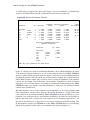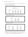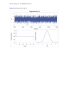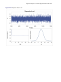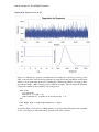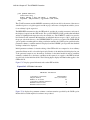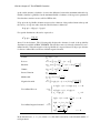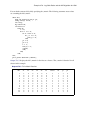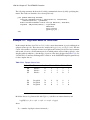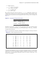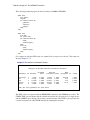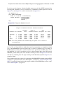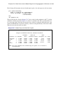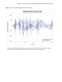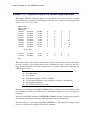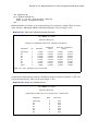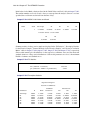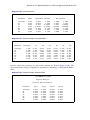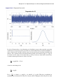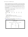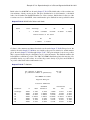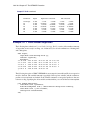
1
® SAS/STAT 9.22 User’s Guide The GENMOD Procedure (Book Excerpt) SAS® Documentation This document is an individual chapter from SAS/STAT® 9.22 User’s Guide. The correct bibliographic citation for the complete manual is as follows: SAS Institute Inc. 2010. SAS/STAT® 9.22 User’s Guide. Cary, NC: SAS Institute Inc. Copyright © 2010, SAS Institute Inc., Cary, NC, USA All rights reserved. Produced in the United States of America. For a Web download or e-book: Your use of this publication shall be governed by the terms established by the vendor at the time you acquire this publication. U.S. Government Restricted Rights Notice: Use, duplication, or disclosure of this software and related documentation by the U.S. government is subject to the Agreement with SAS Institute and the restrictions set forth in FAR 52.227-19, Commercial Computer Software-Restricted Rights (June 1987). SAS Institute Inc., SAS Campus Drive, Cary, North Carolina 27513. 1st electronic book, May 2010 SAS® Publishing provides a complete selection of books and electronic products to help customers use SAS software to its fullest potential. For more information about our e-books, e-learning products, CDs, and hard-copy books, visit the SAS Publishing Web site at support.sas.com/publishing or call 1-800-727-3228. SAS® and all other SAS Institute Inc. product or service names are registered trademarks or trademarks of SAS Institute Inc. in the USA and other countries. ® indicates USA registration. Other brand and product names are registered trademarks or trademarks of their respective companies. Chapter 37 The GENMOD Procedure Contents Overview: GENMOD Procedure . . . . . . . . . . . . . . . . . . . . . . . . . . . 2429 What Is a Generalized Linear Model? . . . . . . . . . . . . . . . . . . . . . 2430 Examples of Generalized Linear Models . . . . . . . . . . . . . . . . . . . . 2431 The GENMOD Procedure . . . . . . . . . . . . . . . . . . . . . . . . . . . 2432 Getting Started: GENMOD Procedure . . . . . . . . . . . . . . . . . . . . . . . . 2435 Poisson Regression . . . . . . . . . . . . . . . . . . . . . . . . . . . . . . 2435 Bayesian Analysis of a Linear Regression Model . . . . . . . . . . . . . . . 2440 Generalized Estimating Equations . . . . . . . . . . . . . . . . . . . . . . . 2453 Syntax: GENMOD Procedure . . . . . . . . . . . . . . . . . . . . . . . . . . . . 2456 PROC GENMOD Statement . . . . . . . . . . . . . . . . . . . . . . . . . . . 2457 ASSESS Statement . . . . . . . . . . . . . . . . . . . . . . . . . . . . . . . 2462 BAYES Statement . . . . . . . . . . . . . . . . . . . . . . . . . . . . . . . 2463 BY Statement . . . . . . . . . . . . . . . . . . . . . . . . . . . . . . . . . 2473 CLASS Statement . . . . . . . . . . . . . . . . . . . . . . . . . . . . . . . 2474 CONTRAST Statement . . . . . . . . . . . . . . . . . . . . . . . . . . . . . 2477 DEVIANCE Statement . . . . . . . . . . . . . . . . . . . . . . . . . . . . 2479 EFFECTPLOT Statement . . . . . . . . . . . . . . . . . . . . . . . . . . . 2480 ESTIMATE Statement . . . . . . . . . . . . . . . . . . . . . . . . . . . . . . 2481 EXACT Statement . . . . . . . . . . . . . . . . . . . . . . . . . . . . . . . EXACTOPTIONS Statement . . . . . . . . . . . . . . . . . . . . . . . . . 2482 2484 FREQ Statement . . . . . . . . . . . . . . . . . . . . . . . . . . . . . . . . . 2487 FWDLINK Statement . . . . . . . . . . . . . . . . . . . . . . . . . . . . . . 2487 INVLINK Statement . . . . . . . . . . . . . . . . . . . . . . . . . . . . . . 2488 LSMEANS Statement . . . . . . . . . . . . . . . . . . . . . . . . . . . . . 2488 LSMESTIMATE Statement . . . . . . . . . . . . . . . . . . . . . . . . . . 2489 MODEL Statement . . . . . . . . . . . . . . . . . . . . . . . . . . . . . . . . 2491 OUTPUT Statement . . . . . . . . . . . . . . . . . . . . . . . . . . . . . . 2499 Programming Statements . . . . . . . . . . . . . . . . . . . . . . . . . . . 2502 REPEATED Statement . . . . . . . . . . . . . . . . . . . . . . . . . . . . . 2503 SLICE Statement . . . . . . . . . . . . . . . . . . . . . . . . . . . . . . . . . 2507 STORE Statement . . . . . . . . . . . . . . . . . . . . . . . . . . . . . . . . 2507 STRATA Statement . . . . . . . . . . . . . . . . . . . . . . . . . . . . . . . 2507 VARIANCE Statement . . . . . . . . . . . . . . . . . . . . . . . . . . . . . 2509 WEIGHT Statement . . . . . . . . . . . . . . . . . . . . . . . . . . . . . . 2509 2428 F Chapter 37: The GENMOD Procedure ZEROMODEL Statement . . . . . . . . . . . . . . . . . . . . . . . . . . . 2510 Details: GENMOD Procedure . . . . . . . . . . . . . . . . . . . . . . . . . . . . 2510 Generalized Linear Models Theory . . . . . . . . . . . . . . . . . . . . . . 2510 Specification of Effects . . . . . . . . . . . . . . . . . . . . . . . . . . . . 2522 Parameterization Used in PROC GENMOD . . . . . . . . . . . . . . . . . . 2523 Type 1 Analysis . . . . . . . . . . . . . . . . . . . . . . . . . . . . . . . . 2523 Type 3 Analysis . . . . . . . . . . . . . . . . . . . . . . . . . . . . . . . . 2524 Confidence Intervals for Parameters . . . . . . . . . . . . . . . . . . . . . . 2525 F Statistics . . . . . . . . . . . . . . . . . . . . . . . . . . . . . . . . . . . 2526 Lagrange Multiplier Statistics . . . . . . . . . . . . . . . . . . . . . . . . . . 2527 Predicted Values of the Mean . . . . . . . . . . . . . . . . . . . . . . . . . . 2527 Residuals . . . . . . . . . . . . . . . . . . . . . . . . . . . . . . . . . . . . 2528 Multinomial Models . . . . . . . . . . . . . . . . . . . . . . . . . . . . . . 2529 Zero-Inflated Models . . . . . . . . . . . . . . . . . . . . . . . . . . . . . . Generalized Estimating Equations . . . . . . . . . . . . . . . . . . . . . . . 2530 2532 Assessment of Models Based on Aggregates of Residuals . . . . . . . . . . . 2541 Case Deletion Diagnostic Statistics . . . . . . . . . . . . . . . . . . . . . . 2544 Bayesian Analysis . . . . . . . . . . . . . . . . . . . . . . . . . . . . . . . 2548 Exact Logistic and Poisson Regression . . . . . . . . . . . . . . . . . . . . 2553 Missing Values . . . . . . . . . . . . . . . . . . . . . . . . . . . . . . . . . 2556 Displayed Output for Classical Analysis . . . . . . . . . . . . . . . . . . . 2556 Displayed Output for Bayesian Analysis . . . . . . . . . . . . . . . . . . . 2564 Displayed Output for Exact Analysis . . . . . . . . . . . . . . . . . . . . . . 2567 ODS Table Names . . . . . . . . . . . . . . . . . . . . . . . . . . . . . . . 2568 ODS Graphics . . . . . . . . . . . . . . . . . . . . . . . . . . . . . . . . . 2572 Examples: GENMOD Procedure . . . . . . . . . . . . . . . . . . . . . . . . . . . 2574 Example 37.1: Logistic Regression . . . . . . . . . . . . . . . . . . . . . . 2574 Example 37.2: Normal Regression, Log Link . . . . . . . . . . . . . . . . 2576 Example 37.3: Gamma Distribution Applied to Life Data . . . . . . . . . . 2579 Example 37.4: Ordinal Model for Multinomial Data . . . . . . . . . . . . . 2582 Example 37.5: GEE for Binary Data with Logit Link Function . . . . . . . 2586 Example 37.6: Log Odds Ratios and the ALR Algorithm . . . . . . . . . . 2589 Example 37.7: Log-Linear Model for Count Data . . . . . . . . . . . . . . 2592 Example 37.8: Model Assessment of Multiple Regression Using Aggregates of Residuals . . . . . . . . . . . . . . . . . . . . . . . . . . . . . . . 2597 Example 37.9: Assessment of a Marginal Model for Dependent Data . . . . 2604 Example 37.10: Bayesian Analysis of a Poisson Regression Model . . . . . 2608 Example 37.11: Exact Poisson Regression . . . . . . . . . . . . . . . . . . 2622 References . . . . . . . . . . . . . . . . . . . . . . . . . . . . . . . . . . . . . . 2626 Overview: GENMOD Procedure F 2429 Overview: GENMOD Procedure The GENMOD procedure fits generalized linear models, as defined by Nelder and Wedderburn (1972). The class of generalized linear models is an extension of traditional linear models that allows the mean of a population to depend on a linear predictor through a nonlinear link function and allows the response probability distribution to be any member of an exponential family of distributions. Many widely used statistical models are generalized linear models. These include classical linear models with normal errors, logistic and probit models for binary data, and log-linear models for multinomial data. Many other useful statistical models can be formulated as generalized linear models by the selection of an appropriate link function and response probability distribution. See McCullagh and Nelder (1989) for a discussion of statistical modeling using generalized linear models. The books by Aitkin et al. (1989) and Dobson (1990) are also excellent references with many examples of applications of generalized linear models. Firth (1991) provides an overview of generalized linear models. Myers, Montgomery, and Vining (2002) provide applications of generalized linear models in the engineering and physical sciences. Collett (2003) and Hilbe (2009) provide comprehensive accounts of generalized linear models when the responses are binary. The analysis of correlated data arising from repeated measurements when the measurements are assumed to be multivariate normal has been studied extensively. However, the normality assumption might not always be reasonable; for example, different methodology must be used in the data analysis when the responses are discrete and correlated. Generalized estimating equations (GEEs) provide a practical method with reasonable statistical efficiency to analyze such data. Liang and Zeger (1986) introduced GEEs as a method of dealing with correlated data when, except for the correlation among responses, the data can be modeled as a generalized linear model. For example, correlated binary and count data in many cases can be modeled in this way. The GENMOD procedure can fit models to correlated responses by the GEE method. You can use PROC GENMOD to fit models with most of the correlation structures from Liang and Zeger (1986) by using GEEs. See Hardin and Hilbe (2003), Diggle, Liang, and Zeger (1994), and Lipsitz et al. (1994) for more details on GEEs. Bayesian analysis of generalized linear models can be requested by using the BAYES statement in the GENMOD procedure. In Bayesian analysis, the model parameters are treated as random variables, and inference about parameters is based on the posterior distribution of the parameters, given the data. The posterior distribution is obtained using Bayes’ theorem as the likelihood function of the data weighted with a prior distribution. The prior distribution enables you to incorporate knowledge or experience of the likely range of values of the parameters of interest into the analysis. If you have no prior knowledge of the parameter values, you can use a noninformative prior distribution, and the results of the Bayesian analysis will be very similar to a classical analysis based on maximum likelihood. A closed form of the posterior distribution is often not feasible, and a Markov chain Monte Carlo method by Gibbs sampling is used to simulate samples from the posterior distribution. See Chapter 7, “Introduction to Bayesian Analysis Procedures,” for an introduction to the basic concepts of Bayesian statistics. Also see the section “Bayesian Analysis: Advantages and Disadvantages” on page 147 for a discussion of the advantages and disadvantages of Bayesian analysis. See Ibrahim, Chen, and Sinha (2001) for a detailed description of Bayesian analysis. 2430 F Chapter 37: The GENMOD Procedure In a Bayesian analysis, a Gibbs chain of samples from the posterior distribution is generated for the model parameters. Summary statistics (mean, standard deviation, quartiles, HPD and credible intervals, correlation matrix) and convergence diagnostics (autocorrelations; Gelman-Rubin, Geweke, Raftery-Lewis, and Heidelberger and Welch tests; the effective sample size; and Monte Carlo standard errors) are computed for each parameter, as well as the correlation matrix and the covariance matrix of the posterior sample. Trace plots, posterior density plots, and autocorrelation function plots that are created using ODS Graphics are also provided for each parameter. The GENMOD procedure enables you to perform exact logistic regression, also called exact conditional binary logistic regression, and exact Poisson regression, also called exact conditional Poisson regression, by specifying one or more EXACT statements. You can test individual parameters or conduct a joint test for several parameters. The procedure computes two exact tests: the exact conditional score test and the exact conditional probability test. You can request exact estimation of specific parameters and corresponding odds ratios where appropriate. Point estimates, standard errors, and confidence intervals are provided. The GENMOD procedure now uses ODS Graphics to create graphs as part of its output. For general information about ODS Graphics, see Chapter 21, “Statistical Graphics Using ODS.” What Is a Generalized Linear Model? A traditional linear model is of the form yi D x0i ˇ C "i where yi is the response variable for the i th observation. The quantity xi is a column vector of covariates, or explanatory variables, for observation i that is known from the experimental setting and is considered to be fixed, or nonrandom. The vector of unknown coefficients ˇ is estimated by a least squares fit to the data y. The "i are assumed to be independent, normal random variables with zero mean and constant variance. The expected value of yi , denoted by i , is i D x0i ˇ While traditional linear models are used extensively in statistical data analysis, there are types of problems such as the following for which they are not appropriate. It might not be reasonable to assume that data are normally distributed. For example, the normal distribution (which is continuous) might not be adequate for modeling counts or measured proportions that are considered to be discrete. If the mean of the data is naturally restricted to a range of values, the traditional linear model might not be appropriate, since the linear predictor x0i ˇ can take on any value. For example, the mean of a measured proportion is between 0 and 1, but the linear predictor of the mean in a traditional linear model is not restricted to this range. It might not be realistic to assume that the variance of the data is constant for all observations. For example, it is not unusual to observe data where the variance increases with the mean of the data. Examples of Generalized Linear Models F 2431 A generalized linear model extends the traditional linear model and is therefore applicable to a wider range of data analysis problems. A generalized linear model consists of the following components: The linear component is defined just as it is for traditional linear models: i D x0i ˇ A monotonic differentiable link function g describes how the expected value of yi is related to the linear predictor i : g.i / D x0i ˇ The response variables yi are independent for i = 1, 2,. . . and have a probability distribution from an exponential family. This implies that the variance of the response depends on the mean through a variance function V : var.yi / D V .i / wi where is a constant and wi is a known weight for each observation. The dispersion parameter is either known (for example, for the binomial or Poisson distribution, D 1) or must be estimated. See the section “Response Probability Distributions” on page 2510 for the form of a probability distribution from the exponential family of distributions. As in the case of traditional linear models, fitted generalized linear models can be summarized through statistics such as parameter estimates, their standard errors, and goodness-of-fit statistics. You can also make statistical inference about the parameters by using confidence intervals and hypothesis tests. However, specific inference procedures are usually based on asymptotic considerations, since exact distribution theory is not available or is not practical for all generalized linear models. Examples of Generalized Linear Models You construct a generalized linear model by deciding on response and explanatory variables for your data and choosing an appropriate link function and response probability distribution. Some examples of generalized linear models follow. Explanatory variables can be any combination of continuous variables, classification variables, and interactions. Traditional Linear Model response variable: a continuous variable distribution: normal link function: identity g./ D 2432 F Chapter 37: The GENMOD Procedure Logistic Regression response variable: a proportion distribution: binomial link function: logit g./ D log 1 Poisson Regression in Log-Linear Model response variable: a count distribution: Poisson link function: log g./ D log./ Gamma Model with Log Link response variable: a positive, continuous variable distribution: gamma link function: log g./ D log./ The GENMOD Procedure The GENMOD procedure fits a generalized linear model to the data by maximum likelihood estimation of the parameter vector ˇ. There is, in general, no closed form solution for the maximum likelihood estimates of the parameters. The GENMOD procedure estimates the parameters of the model numerically through an iterative fitting process. The dispersion parameter is also estimated by maximum likelihood or, optionally, by the residual deviance or by Pearson’s chi-square divided by the degrees of freedom. Covariances, standard errors, and p-values are computed for the estimated parameters based on the asymptotic normality of maximum likelihood estimators. A number of popular link functions and probability distributions are available in the GENMOD procedure. The built-in link functions are as follows: identity: g./ D logit: g./ D log.=.1 // probit: g./ D ˆ 1 ./, where ˆ is the standard normal cumulative distribution function if ¤ 0 power: g./ D log./ if D 0 log: g./ D log./ The GENMOD Procedure F 2433 complementary log-log: g./ D log. log.1 // The available distributions and associated variance functions are as follows: normal: V ./ D 1 binomial (proportion): V ./ D .1 / Poisson: V ./ D gamma: V ./ D 2 inverse Gaussian: V ./ D 3 negative binomial: V ./ D C k2 geometric: V ./ D C 2 multinomial zero-inflated Poisson zero-inflated negative binomial The negative binomial and zero-inflated negative binomial are distributions with an additional parameter k in the variance function. PROC GENMOD estimates k by maximum likelihood, or you can optionally set it to a constant value. See McCullagh and Nelder (1989), Hilbe (1994), Hilbe (2007), Long (1997), Cameron and Trivedi (1998), or Lawless (1987) for discussions of the negative binomial distribution. The multinomial distribution is sometimes used to model a response that can take values from a number of categories. The binomial is a special case of the multinomial with two categories. See the section “Multinomial Models” on page 2529 and McCullagh and Nelder (1989, Chapter 5) for a description of the multinomial distribution. The zero-inflated Poisson and zero-inflated negative binomial are included in PROC GENMOD even though they are not generalized linear models. They are useful extensions of generalized linear models. See the section “Zero-Inflated Models” on page 2530 for information about the zero-inflated distributions. In addition, you can easily define your own link functions or distributions through DATA step programming statements used within the procedure. An important aspect of generalized linear modeling is the selection of explanatory variables in the model. Changes in goodness-of-fit statistics are often used to evaluate the contribution of subsets of explanatory variables to a particular model. The deviance, defined to be twice the difference between the maximum attainable log likelihood and the log likelihood of the model under consideration, is often used as a measure of goodness of fit. The maximum attainable log likelihood is achieved with a model that has a parameter for every observation. See the section “Goodness of Fit” on page 2517 for formulas for the deviance. One strategy for variable selection is to fit a sequence of models, beginning with a simple model with only an intercept term, and then to include one additional explanatory variable in each successive 2434 F Chapter 37: The GENMOD Procedure model. You can measure the importance of the additional explanatory variable by the difference in deviances or fitted log likelihoods between successive models. Asymptotic tests computed by the GENMOD procedure enable you to assess the statistical significance of the additional term. The GENMOD procedure enables you to fit a sequence of models, up through a maximum number of terms specified in a MODEL statement. A table summarizes twice the difference in log likelihoods between each successive pair of models. This is called a Type 1 analysis in the GENMOD procedure, because it is analogous to Type I (sequential) sums of squares in the GLM procedure. As with the PROC GLM Type I sums of squares, the results from this process depend on the order in which the model terms are fit. The GENMOD procedure also generates a Type 3 analysis analogous to Type III sums of squares in the GLM procedure. A Type 3 analysis does not depend on the order in which the terms for the model are specified. A GENMOD procedure Type 3 analysis consists of specifying a model and computing likelihood ratio statistics for Type III contrasts for each term in the model. The contrasts are defined in the same way as they are in the GLM procedure. The GENMOD procedure optionally computes Wald statistics for Type III contrasts. This is computationally less expensive than likelihood ratio statistics, but it is thought to be less accurate because the specified significance level of hypothesis tests based on the Wald statistic might not be as close to the actual significance level as it is for likelihood ratio tests. A Type 3 analysis generalizes the use of Type III estimable functions in linear models. Briefly, a Type III estimable function (contrast) for an effect is a linear function of the model parameters that involves the parameters of the effect and any interactions with that effect. A test of the hypothesis that the Type III contrast for a main effect is equal to 0 is intended to test the significance of the main effect in the presence of interactions. See Chapter 39, “The GLM Procedure,” and Chapter 15, “The Four Types of Estimable Functions,” for more information about Type III estimable functions. Also refer to Littell, Freund, and Spector (1991). Additional features of the GENMOD procedure include the following: likelihood ratio statistics for user-defined contrasts—that is, linear functions of the parameters and p-values based on their asymptotic chi-square distributions estimated values, standard errors, and confidence limits for user-defined contrasts and least squares means ability to create a SAS data set corresponding to most tables displayed by the procedure (see Table 37.8 and Table 37.9) confidence intervals for model parameters based on either the profile likelihood function or asymptotic normality syntax similar to that of PROC GLM for the specification of the response and model effects, including interaction terms and automatic coding of classification variables ability to fit GEE models for clustered response data ability to perform Bayesian analysis by Gibbs sampling Getting Started: GENMOD Procedure F 2435 Getting Started: GENMOD Procedure Poisson Regression You can use the GENMOD procedure to fit a variety of statistical models. A typical use of PROC GENMOD is to perform Poisson regression. You can use the Poisson distribution to model the distribution of cell counts in a multiway contingency table. Aitkin et al. (1989) have used this method to model insurance claims data. Suppose the following hypothetical insurance claims data are classified by two factors: age group (with two levels) and car type (with three levels). data insure; input n c car$ age; ln = log(n); datalines; 500 42 small 1 1200 37 medium 1 100 1 large 1 400 101 small 2 500 73 medium 2 300 14 large 2 ; run; In the preceding data set, the variable n represents the number of insurance policyholders and the variable c represents the number of insurance claims. The variable car is the type of car involved (classified into three groups) and the variable age is the age group of a policyholder (classified into two groups). You can use PROC GENMOD to perform a Poisson regression analysis of these data with a log link function. This type of model is sometimes called a log-linear model. Assume that the number of claims c has a Poisson probability distribution and that its mean, i , is related to the factors car and age for observation i by log.i / D log.ni / C x0i ˇ D log.ni / C ˇ0 C cari .1/ˇ1 C cari .2/ˇ2 C cari .3/ˇ3 C agei .1/ˇ4 C agei .2/ˇ5 The indicator variables cari .j / and agei .j / are associated with the j th level of the variables car and 2436 F Chapter 37: The GENMOD Procedure age for observation i cari .j / D 1 if car D j 0 if car ¤ j The ˇs are unknown parameters to be estimated by the procedure. The logarithm of the variable n is used as an offset—that is, a regression variable with a constant coefficient of 1 for each observation. A log-linear relationship between the mean and the factors car and age is specified by the log link function. The log link function ensures that the mean number of insurance claims for each car and age group predicted from the fitted model is positive. The following statements invoke the GENMOD procedure to perform this analysis: proc genmod data=insure; class car age; model c = car age / dist = poisson link = log offset = ln; run; The variables car and age are specified as CLASS variables so that PROC GENMOD automatically generates the indicator variables associated with car and age. The MODEL statement specifies c as the response variable and car and age as explanatory variables. An intercept term is included by default. Thus, the model matrix X (the matrix that has as its i th row the transpose of the covariate vector for the i th observation) consists of a column of 1s representing the intercept term and columns of 0s and 1s derived from indicator variables representing the levels of the car and age variables. That is, the model matrix is 2 1 1 0 0 6 1 0 1 0 6 6 1 0 0 1 XD6 6 1 1 0 0 6 4 1 0 1 0 1 0 0 1 1 1 1 0 0 0 0 0 0 1 1 1 3 7 7 7 7 7 7 5 where the first column corresponds to the intercept, the next three columns correspond to the variable car, and the last two columns correspond to the variable age. The response distribution is specified as Poisson, and the link function is chosen to be log. That is, the Poisson mean parameter is related to the linear predictor by log./ D x0i ˇ The logarithm of n is specified as an offset variable, as is common in this type of analysis. In this case, the offset variable serves to normalize the fitted cell means to a per-policyholder basis, since the total number of claims, not individual policyholder claims, is observed. Poisson Regression F 2437 PROC GENMOD produces the following default output from the preceding statements. Figure 37.1 Model Information The GENMOD Procedure Model Information Data Set Distribution Link Function Dependent Variable Offset Variable WORK.INSURE Poisson Log c ln The “Model Information” table displayed in Figure 37.1 provides information about the specified model and the input data set. Figure 37.2 Class Level Information Class Level Information Class Levels car age Values 3 2 large medium small 1 2 Figure 37.2 displays the “Class Level Information” table, which identifies the levels of the classification variables that are used in the model. Note that car is a character variable, and the values are sorted in alphabetical order. This is the default sort order, but you can select different sort orders with the ORDER= option in the PROC GENMOD statement. Figure 37.3 Goodness of Fit Criteria For Assessing Goodness Of Fit Criterion Deviance Scaled Deviance Pearson Chi-Square Scaled Pearson X2 Log Likelihood Full Log Likelihood AIC (smaller is better) AICC (smaller is better) BIC (smaller is better) DF Value Value/DF 2 2 2 2 2.8207 2.8207 2.8416 2.8416 837.4533 -16.4638 40.9276 80.9276 40.0946 1.4103 1.4103 1.4208 1.4208 The “Criteria For Assessing Goodness Of Fit” table displayed in Figure 37.3 contains statistics that summarize the fit of the specified model. These statistics are helpful in judging the adequacy of a model and in comparing it with other models under consideration. If you compare the deviance 2438 F Chapter 37: The GENMOD Procedure of 2.8207 with its asymptotic chi-square with 2 degrees of freedom distribution, you find that the p-value is 0.24. This indicates that the specified model fits the data reasonably well. Figure 37.4 Analysis of Parameter Estimates Analysis Of Maximum Likelihood Parameter Estimates Parameter Intercept car car car age age Scale large medium small 1 2 DF Estimate Standard Error 1 1 1 0 1 0 0 -1.3168 -1.7643 -0.6928 0.0000 -1.3199 0.0000 1.0000 0.0903 0.2724 0.1282 0.0000 0.1359 0.0000 0.0000 Wald 95% Confidence Limits -1.4937 -2.2981 -0.9441 0.0000 -1.5863 0.0000 1.0000 -1.1398 -1.2304 -0.4414 0.0000 -1.0536 0.0000 1.0000 Wald Chi-Square 212.73 41.96 29.18 . 94.34 . Analysis Of Maximum Likelihood Parameter Estimates Parameter Intercept car car car age age Scale Pr > ChiSq large medium small 1 2 <.0001 <.0001 <.0001 . <.0001 . NOTE: The scale parameter was held fixed. Figure 37.4 displays the “Analysis Of Parameter Estimates” table, which summarizes the results of the iterative parameter estimation process. For each parameter in the model, PROC GENMOD displays columns with the parameter name, the degrees of freedom associated with the parameter, the estimated parameter value, the standard error of the parameter estimate, the confidence intervals, and the Wald chi-square statistic and associated p-value for testing the significance of the parameter to the model. If a column of the model matrix corresponding to a parameter is found to be linearly dependent, or aliased, with columns corresponding to parameters preceding it in the model, PROC GENMOD assigns it zero degrees of freedom and displays a value of zero for both the parameter estimate and its standard error. This table includes a row for a scale parameter, even though there is no free scale parameter in the Poisson distribution. See the section “Response Probability Distributions” on page 2510 for the form of the Poisson probability distribution. PROC GENMOD allows the specification of a scale parameter to fit overdispersed Poisson and binomial distributions. In such cases, the SCALE row indicates the value of the overdispersion scale parameter used in adjusting output statistics. See the section “Overdispersion” on page 2521 for more about overdispersion and the meaning of the SCALE parameter output by the GENMOD procedure. PROC GENMOD displays a note indicating that the scale parameter is fixed—that is, not estimated by the iterative fitting process. Poisson Regression F 2439 It is usually of interest to assess the importance of the main effects in the model. Type 1 and Type 3 analyses generate statistical tests for the significance of these effects. You can request these analyses with the TYPE1 and TYPE3 options in the MODEL statement, as follows: proc genmod data=insure; class car age; model c = car age / dist = poisson link = log offset = ln type1 type3; run; The results of these analyses are summarized in the figures that follow. Figure 37.5 Type 1 Analysis The GENMOD Procedure LR Statistics For Type 1 Analysis Source Deviance DF ChiSquare Pr > ChiSq Intercept car age 175.1536 107.4620 2.8207 2 1 67.69 104.64 <.0001 <.0001 In the table for Type 1 analysis displayed in Figure 37.5, each entry in the deviance column represents the deviance for the model containing the effect for that row and all effects preceding it in the table. For example, the deviance corresponding to car in the table is the deviance of the model containing an intercept and car. As more terms are included in the model, the deviance decreases. Entries in the chi-square column are likelihood ratio statistics for testing the significance of the effect added to the model containing all the preceding effects. The chi-square value of 67.69 for car represents twice the difference in log likelihoods between fitting a model with only an intercept term and a model with an intercept and car. Since the scale parameter is set to 1 in this analysis, this is equal to the difference in deviances. Since two additional parameters are involved, this statistic can be compared with a chi-square distribution with two degrees of freedom. The resulting p-value (labeled Pr>Chi) of less than 0.0001 indicates that this variable is highly significant. Similarly, the chi-square value of 104.64 for age represents the difference in log likelihoods between the model with the intercept and car and the model with the intercept, car, and age. This effect is also highly significant, as indicated by the small p-value. 2440 F Chapter 37: The GENMOD Procedure Figure 37.6 Type 3 Analysis LR Statistics For Type 3 Analysis Source car age DF ChiSquare Pr > ChiSq 2 1 72.82 104.64 <.0001 <.0001 The Type 3 analysis results in the same conclusions as the Type 1 analysis. The Type 3 chi-square value for the car variable, for example, is twice the difference between the log likelihood for the model with the variables Intercept, car, and age included and the log likelihood for the model with the car variable excluded. The hypothesis tested in this case is the significance of the variable car given that the variable age is in the model. In other words, it tests the additional contribution of car in the model. The values of the Type 3 likelihood ratio statistics for the car and age variables indicate that both of these factors are highly significant in determining the claims performance of the insurance policyholders. Bayesian Analysis of a Linear Regression Model Neter et al. (1996) describe a study of 54 patients undergoing a certain kind of liver operation in a surgical unit. The data set Surg contains survival time and certain covariates for each patient. Observations for the first 20 patients in the data set Surg are shown in Figure 37.7. Bayesian Analysis of a Linear Regression Model F 2441 Figure 37.7 Surgical Unit Data Obs x1 x2 x3 x4 y logy Logx1 1 2 3 4 5 6 7 8 9 10 11 12 13 14 15 16 17 18 19 20 6.7 5.1 7.4 6.5 7.8 5.8 5.7 3.7 6.0 3.7 6.3 6.7 5.8 5.8 7.7 7.4 6.0 3.7 7.3 5.6 62 59 57 73 65 38 46 68 67 76 84 51 96 83 62 74 85 51 68 57 81 66 83 41 115 72 63 81 93 94 83 43 114 88 67 68 28 41 74 87 2.59 1.70 2.16 2.01 4.30 1.42 1.91 2.57 2.50 2.40 4.13 1.86 3.95 3.95 3.40 2.40 2.98 1.55 3.56 3.02 200 101 204 101 509 80 80 127 202 203 329 65 830 330 168 217 87 34 215 172 2.3010 2.0043 2.3096 2.0043 2.7067 1.9031 1.9031 2.1038 2.3054 2.3075 2.5172 1.8129 2.9191 2.5185 2.2253 2.3365 1.9395 1.5315 2.3324 2.2355 1.90211 1.62924 2.00148 1.87180 2.05412 1.75786 1.74047 1.30833 1.79176 1.30833 1.84055 1.90211 1.75786 1.75786 2.04122 2.00148 1.79176 1.30833 1.98787 1.72277 Consider the model Y D ˇ0 C ˇ1 LogX1 C ˇ2 X 2 C ˇ3 X 3 C ˇ4 X 4 C where Y is the survival time, LogX1 is log(blood-clotting score), X2 is a prognostic index, X3 is an enzyme function test score, X4 is a liver function test score, and is an N.0; 2 / error term. A question of scientific interest is whether blood clotting score has a positive effect on survival time. Using PROC GENMOD, you can obtain a maximum likelihood estimate of the coefficient and construct a null point hypothesis to test whether ˇ1 is equal to 0. However, if you are interested in finding the probability that the coefficient is positive, Bayesian analysis offers a convenient alternative. You can use Bayesian analysis to directly estimate the conditional probability, Pr.ˇ1 > 0jY/, using the posterior distribution samples, which are produced as part of the output by PROC GENMOD. The example that follows shows how to use PROC GENMOD to carry out a Bayesian analysis of the linear model with a normal error term. The SEED= option is specified to maintain reproducibility; no other options are specified in the BAYES statement. By default, a uniform prior distribution is assumed on the regression coefficients. The uniform prior is a flat prior on the real line with a distribution that reflects ignorance of the location of the parameter, placing equal likelihood on all possible values the regression coefficient can take. Using the uniform prior in the following example, you would expect the Bayesian estimates to resemble the classical results of maximizing the likelihood. If you can elicit an informative prior distribution for the regression coefficients, you should use the COEFFPRIOR= option to specify it. A default noninformative gamma prior is used for the scale parameter . 2442 F Chapter 37: The GENMOD Procedure You should make sure that the posterior distribution samples have achieved convergence before using them for Bayesian inference. PROC GENMOD produces three convergence diagnostics by default. If ODS Graphics is enabled as specified in the following SAS statements, diagnostic plots are also displayed. See the section “Assessing Markov Chain Convergence” on page 155 for more information about convergence diagnostics and their interpretation. Summary statistics of the posterior distribution samples are produced by default. However, these statistics might not be sufficient for carrying out your Bayesian inference, and further processing of the posterior samples might be necessary. The following SAS statements request the Bayesian analysis, and the OUTPOST= option saves the samples in the SAS data set PostSurg for further processing: ods graphics on; proc genmod data=Surg; model y = Logx1 X2 X3 X4 / dist=normal; bayes seed=1 OutPost=PostSurg; run; ods graphics off; The results of this analysis are shown in the following figures. The “Model Information” table in Figure 37.8 summarizes information about the model you fit and the size of the simulation. Figure 37.8 Model Information The GENMOD Procedure Bayesian Analysis Model Information Data Set Burn-In Size MC Sample Size Thinning Sampling Algorithm Distribution Link Function Dependent Variable WORK.SURG 2000 10000 1 Conjugate Normal Identity y Survival Time Bayesian Analysis of a Linear Regression Model F 2443 The “Analysis of Maximum Likelihood Parameter Estimates” table in Figure 37.9 summarizes maximum likelihood estimates of the model parameters. Figure 37.9 Maximum Likelihood Parameter Estimates Analysis Of Maximum Likelihood Parameter Estimates Parameter DF Estimate Standard Error Intercept Logx1 x2 x3 x4 Scale 1 1 1 1 1 1 -730.559 171.8758 4.3019 4.0309 18.1377 59.8591 85.4333 38.2250 0.5566 0.4996 12.0721 5.7599 Wald 95% Confidence Limits -898.005 96.9561 3.2109 3.0517 -5.5232 49.5705 -563.112 246.7954 5.3929 5.0100 41.7986 72.2832 NOTE: The scale parameter was estimated by maximum likelihood. Since no prior distributions for the regression coefficients were specified, the default noninformative uniform distributions shown in the “Uniform Prior for Regression Coefficients” table in Figure 37.10 are used. Noninformative priors are appropriate if you have no prior knowledge of the likely range of values of the parameters, and if you want to make probability statements about the parameters or functions of the parameters. See, for example, Ibrahim, Chen, and Sinha (2001) for more information about choosing prior distributions. Figure 37.10 Regression Coefficient Priors The GENMOD Procedure Bayesian Analysis Uniform Prior for Regression Coefficients Parameter Prior Intercept Logx1 x2 x3 x4 Constant Constant Constant Constant Constant 2444 F Chapter 37: The GENMOD Procedure The default noninformative gamma prior distribution for the normal scale parameter is shown in the “Independent Prior Distributions for Model Parameters” table in Figure 37.11. Figure 37.11 Scale Parameter Prior Independent Prior Distributions for Model Parameters Parameter Prior Distribution Hyperparameters Shape Scale Dispersion Inverse Gamma 2.001 0.0001 By default, the maximum likelihood estimates of the regression parameters are used as the starting values for the simulation when noninformative prior distributions are used. These are listed in the “Initial Values and Seeds” table in Figure 37.12. Figure 37.12 MCMC Initial Values and Seeds Initial Values of the Chain Chain Seed Intercept Logx1 x2 x3 x4 1 1 -730.559 171.8758 4.301896 4.030878 18.1377 Initial Values of the Chain Dispersion 3223.694 Summary statistics for the posterior sample are displayed in the “Fit Statistics,” “Descriptive Statistics for the Posterior Sample,” “Interval Statistics for the Posterior Sample,” and “Posterior Correlation Matrix” tables in Figure 37.13, Figure 37.14, Figure 37.15, and Figure 37.16, respectively. Figure 37.13 Fit Statistics Fit Statistics DIC (smaller is better) pD (effective number of parameters) 608.411 6.571 Bayesian Analysis of a Linear Regression Model F 2445 Figure 37.14 Descriptive Statistics The GENMOD Procedure Bayesian Analysis Posterior Summaries Parameter Intercept Logx1 x2 x3 x4 Dispersion N Mean Standard Deviation 25% 10000 10000 10000 10000 10000 10000 -730.1 171.7 4.3000 4.0310 18.0888 3795.9 91.0133 40.3792 0.5989 0.5354 12.8949 770.4 -789.6 144.3 3.8990 3.6645 9.4919 3247.6 Percentiles 50% -729.6 171.8 4.2932 4.0265 18.0430 3694.7 75% -670.5 198.6 4.6951 4.3910 26.7881 4238.2 Figure 37.15 Interval Statistics Posterior Intervals Parameter Alpha Equal-Tail Interval Intercept Logx1 x2 x3 x4 Dispersion 0.050 0.050 0.050 0.050 0.050 0.050 -908.7 92.4773 3.1062 2.9812 -7.2646 2569.0 HPD Interval -551.0 251.6 5.4839 5.1041 43.6506 5548.5 -906.2 94.2813 3.1747 2.9532 -5.9839 2389.4 -549.2 253.0 5.5328 5.0612 44.6427 5308.8 Figure 37.16 Posterior Sample Correlation Matrix Posterior Correlation Matrix Parameter Intercept Logx1 x2 x3 x4 Dispersion Intercept Logx1 x2 x3 x4 Dispersion 1.000 -0.856 -0.580 -0.712 0.579 -0.002 -0.856 1.000 0.285 0.490 -0.636 0.009 -0.580 0.285 1.000 0.302 -0.492 -0.007 -0.712 0.490 0.302 1.000 -0.616 -0.004 0.579 -0.636 -0.492 -0.616 1.000 0.002 -0.002 0.009 -0.007 -0.004 0.002 1.000 Since noninformative prior distributions were used, the posterior sample means, standard deviations, and interval statistics shown in Figure 37.13 and Figure 37.14 are consistent with the maximum likelihood estimates shown in Figure 37.9. By default, PROC GENMOD computes three convergence diagnostics: the lag1, lag5, lag10, and lag50 autocorrelations (Figure 37.17); Geweke diagnostic statistics (Figure 37.18); and effective sample sizes (Figure 37.19). There is no indication that the Markov chain has not converged. 2446 F Chapter 37: The GENMOD Procedure See the section “Assessing Markov Chain Convergence” on page 155 for more information about convergence diagnostics and their interpretation. Figure 37.17 Posterior Sample Autocorrelations The GENMOD Procedure Bayesian Analysis Posterior Autocorrelations Parameter Intercept Logx1 x2 x3 x4 Dispersion Lag 1 Lag 5 Lag 10 Lag 50 -0.0050 0.0030 -0.0113 0.0019 -0.0001 -0.0019 -0.0023 -0.0063 -0.0046 0.0064 -0.0084 0.0088 -0.0138 -0.0070 -0.0235 -0.0073 0.0050 -0.0297 0.0032 -0.0034 -0.0139 0.0047 -0.0084 0.0025 Figure 37.18 Geweke Diagnostic Statistics Geweke Diagnostics Parameter Intercept Logx1 x2 x3 x4 Dispersion z Pr > |z| -0.8783 1.4800 -0.0438 0.1000 -0.8893 0.1011 0.3798 0.1389 0.9651 0.9204 0.3739 0.9195 Figure 37.19 Effective Sample Sizes Effective Sample Sizes Parameter Intercept Logx1 x2 x3 x4 Dispersion ESS Autocorrelation Time Efficiency 10000.0 10000.0 10232.2 10000.0 10000.0 10000.0 1.0000 1.0000 0.9773 1.0000 1.0000 1.0000 1.0000 1.0000 1.0232 1.0000 1.0000 1.0000 Trace, autocorrelation, and density plots for the seven model parameters, shown in Figure 37.20 through Figure 37.25, are useful in diagnosing whether the Markov chain of posterior samples has converged. These plots show no evidence that the chain has not converged. See the section “Visual Analysis via Trace Plots” on page 155 for help with interpreting these diagnostic plots. Bayesian Analysis of a Linear Regression Model F 2447 Figure 37.20 Diagnostic Plots for Intercept 2448 F Chapter 37: The GENMOD Procedure Figure 37.21 Diagnostic Plots for logX1 Bayesian Analysis of a Linear Regression Model F 2449 Figure 37.22 Diagnostic Plots for X2 2450 F Chapter 37: The GENMOD Procedure Figure 37.23 Diagnostic Plots for X3 Bayesian Analysis of a Linear Regression Model F 2451 Figure 37.24 Diagnostic Plots for X4 2452 F Chapter 37: The GENMOD Procedure Figure 37.25 Diagnostic Plots for X5 Suppose, for illustration, a question of scientific interest is whether blood clotting score has a positive effect on survival time. Since the model parameters are regarded as random quantities in a Bayesian analysis, you can answer this question by estimating the conditional probability of ˇ1 being positive, given the data, Pr.ˇ1 > 0jY/, from the posterior distribution samples. The following SAS statements compute the estimate of the probability of ˇ1 being positive: data Prob; set PostSurg; Indicator = (logX1 > 0); label Indicator= 'log(Blood Clotting Score) > 0'; run; proc Means data = Prob(keep=Indicator) n mean; run; As shown in Figure 37.26, there is a 1.00 probability of a positive relationship between the logarithm of a blood clotting score and survival time, adjusted for the other covariates. Generalized Estimating Equations F 2453 Figure 37.26 Probability That ˇ1 > 0 The MEANS Procedure Analysis Variable : Indicator log(Blood Clotting Score) > 0 N Mean --------------------10000 0.9999000 --------------------- Generalized Estimating Equations This section illustrates the use of the REPEATED statement to fit a GEE model, using repeated measures data from the “Six Cities” study of the health effects of air pollution (Ware et al. 1984). The data analyzed are the 16 selected cases in Lipsitz et al. (1994). The binary response is the wheezing status of 16 children at ages 9, 10, 11, and 12 years. The mean response is modeled as a logistic regression model by using the explanatory variables city of residence, age, and maternal smoking status at the particular age. The binary responses for individual children are assumed to be equally correlated, implying an exchangeable correlation structure. The data set and SAS statements that fit the model by the GEE method are as follows: data six; input case city$ @@; do i=1 to 4; input age smoke wheeze @@; output; end; datalines; 1 portage 9 0 1 10 0 1 11 0 1 2 kingston 9 1 1 10 2 1 11 2 0 3 kingston 9 0 1 10 0 0 11 1 0 4 portage 9 0 0 10 0 1 11 0 1 5 kingston 9 0 0 10 1 0 11 1 0 6 portage 9 0 0 10 1 0 11 1 0 7 kingston 9 1 0 10 1 0 11 0 0 8 portage 9 1 0 10 1 0 11 1 0 9 portage 9 2 1 10 2 0 11 1 0 10 kingston 9 0 0 10 0 0 11 0 0 11 kingston 9 1 1 10 0 0 11 0 1 12 portage 9 1 0 10 0 0 11 0 0 13 kingston 9 1 0 10 0 1 11 1 1 14 portage 9 1 0 10 2 0 11 1 0 15 kingston 9 1 0 10 1 0 11 1 0 16 portage 9 1 1 10 1 1 11 2 0 ; run; 12 0 0 12 2 0 12 1 0 12 1 0 12 1 0 12 1 0 12 0 0 12 2 0 12 1 0 12 1 0 12 0 1 12 0 0 12 1 1 12 2 1 12 2 1 12 1 0 2454 F Chapter 37: The GENMOD Procedure proc genmod data=six ; class case city ; model wheeze = city age smoke / dist=bin; repeated subject=case / type=exch covb corrw; run; The CLASS statement and the MODEL statement specify the model for the mean of the wheeze variable response as a logistic regression with city, age, and smoke as independent variables, just as for an ordinary logistic regression. The REPEATED statement invokes the GEE method, specifies the correlation structure, and controls the displayed output from the GEE model. The option SUBJECT=CASE specifies that individual subjects be identified in the input data set by the variable case. The SUBJECT= variable case must be listed in the CLASS statement. Measurements on individual subjects at ages 9, 10, 11, and 12 are in the proper order in the data set, so the WITHINSUBJECT= option is not required. The TYPE=EXCH option specifies an exchangeable working correlation structure, the COVB option specifies that the parameter estimate covariance matrix be displayed, and the CORRW option specifies that the final working correlation be displayed. Initial parameter estimates for iterative fitting of the GEE model are computed as in an ordinary generalized linear model, as described previously. Results of the initial model fit displayed as part of the generated output are not shown here. Statistics for the initial model fit such as parameter estimates, standard errors, deviances, and Pearson chi-squares do not apply to the GEE model and are valid only for the initial model fit. The following figures display information that applies to the GEE model fit. Figure 37.27 displays general information about the GEE model fit. Figure 37.27 GEE Model Information The GENMOD Procedure GEE Model Information Correlation Structure Subject Effect Number of Clusters Correlation Matrix Dimension Maximum Cluster Size Minimum Cluster Size Exchangeable case (16 levels) 16 4 4 4 Figure 37.28 displays the parameter estimate covariance matrices specified by the COVB option. Both model-based and empirical covariances are produced. Generalized Estimating Equations F 2455 Figure 37.28 GEE Parameter Estimate Covariance Matrices Covariance Matrix (Model-Based) Prm1 Prm2 Prm4 Prm5 Prm1 Prm2 Prm4 Prm5 5.74947 -0.22257 -0.53472 0.01655 -0.22257 0.45478 -0.002410 0.01876 -0.53472 -0.002410 0.05300 -0.01658 0.01655 0.01876 -0.01658 0.19104 Covariance Matrix (Empirical) Prm1 Prm2 Prm4 Prm5 Prm1 Prm2 Prm4 Prm5 9.33994 -0.85104 -0.83253 -0.16534 -0.85104 0.47368 0.05736 0.04023 -0.83253 0.05736 0.07778 -0.002364 -0.16534 0.04023 -0.002364 0.13051 The exchangeable working correlation matrix specified by the CORRW option is displayed in Figure 37.29. Figure 37.29 GEE Working Correlation Matrix Working Correlation Matrix Row1 Row2 Row3 Row4 Col1 Col2 Col3 Col4 1.0000 0.1648 0.1648 0.1648 0.1648 1.0000 0.1648 0.1648 0.1648 0.1648 1.0000 0.1648 0.1648 0.1648 0.1648 1.0000 The parameter estimates table, displayed in Figure 37.30, contains parameter estimates, standard errors, confidence intervals, Z scores, and p-values for the parameter estimates. Empirical standard error estimates are used in this table. A table that displays model-based standard errors can be created by using the REPEATED statement option MODELSE. Figure 37.30 GEE Parameter Estimates Table Analysis Of GEE Parameter Estimates Empirical Standard Error Estimates Parameter Intercept city kingston city portage age smoke Estimate Standard Error -1.2751 -0.1223 0.0000 0.2036 0.0935 3.0561 0.6882 0.0000 0.2789 0.3613 95% Confidence Limits -7.2650 -1.4713 0.0000 -0.3431 -0.6145 4.7148 1.2266 0.0000 0.7502 0.8016 Z Pr > |Z| -0.42 -0.18 . 0.73 0.26 0.6765 0.8589 . 0.4655 0.7957 2456 F Chapter 37: The GENMOD Procedure Syntax: GENMOD Procedure You can specify the following statements in the GENMOD procedure. Items within the < > are optional. PROC GENMOD < options > ; ASSESS | ASSESSMENT VAR=(effect) | LINK < / options > ; BAYES < options > ; BY variables ; CLASS variable < (options) >: : :< variable < (options) > > < / options > ; CONTRAST ’label’ contrast-specification < / options > ; DEVIANCE variable = expression ; EFFECTPLOT < plot-type < (plot-definition-options) > > < / options > ; ESTIMATE ’label’ effect values < ,. . . effect values > < / options > ; EXACT < ’label’ > < INTERCEPT > < effects > < / options > ; EXACTOPTIONS options ; FREQ | FREQUENCY variable ; FWDLINK variable = expression ; INVLINK variable = expression ; LSMEANS < model-effects > < / options > ; LSMESTIMATE model-effect < ‘label’ > values < divisor =n > < , . . . < ‘label’ > values < divisor =n > > < / options > ; MODEL response = < effects > < / options > ; OUTPUT < OUT=SAS-data-set > < keyword=name. . . keyword=name > ; Programming statements ; REPEATED SUBJECT=subject-effect < / options > ; SLICE model-effect < / options > ; STORE < OUT= >item-store-name < / LABEL=‘label’ > ; STRATA variable < (option) > : : : < variable < (option) > > < / options > ; WEIGHT | SCWGT variable ; VARIANCE variable = expression ; ZEROMODEL < effects > < / options > ; The ASSESS, BAYES, BY, CLASS, CONTRAST, DEVIANCE, ESTIMATE, FREQUENCY, FWDLINK, INVLINK, MODEL, OUTPUT, programming statements, REPEATED, VARIANCE, WEIGHT, and ZEROMODEL statements are described in full after the PROC GENMOD statement in alphabetical order. The EFFECTPLOT, LSMEANS, LSMESTIMATE, SLICE, and STORE statements are common to many procedures. Summary descriptions of functionality and syntax for these statements are also given after the PROC GENMOD statement in alphabetical order, and full documentation about them is available in Chapter 19, “Shared Concepts and Topics.” The PROC GENMOD statement invokes the procedure. All statements other than the MODEL statement are optional. The CLASS statement, if present, must precede the MODEL statement, and the CONTRAST and EXACT statements must come after the MODEL statement. PROC GENMOD Statement F 2457 PROC GENMOD Statement PROC GENMOD < options > ; The PROC GENMOD statement invokes the procedure. You can specify the following options. DATA=SAS-data-set specifies the SAS data set containing the data to be analyzed. If you omit the DATA= option, the procedure uses the most recently created SAS data set. DESCENDING DESCEND DESC specifies that the levels of the response variable for the ordinal multinomial model and the binomial model with single variable response syntax be sorted in the reverse of the default order. For example, if RORDER=FORMATTED (the default), the DESCENDING option causes the levels to be sorted from highest to lowest instead of from lowest to highest. If RORDER=FREQ, the DESCENDING option causes the levels to be sorted from lowest frequency count to highest instead of from highest to lowest. EXACTONLY requests only the exact analyses. The asymptotic analysis that PROC GENMOD usually performs is suppressed. NAMELEN=n specifies the length of effect names in tables and output data sets to be n characters long, where n is a value between 20 and 200 characters. The default length is 20 characters. ORDER=DATA | FORMATTED | FREQ | INTERNAL specifies the order in which to sort the levels of the classification variables (which are specified in the CLASS statement). The ORDER= option can be useful when you use the CONTRAST or ESTIMATE statement because it determines which parameters in the model correspond to each level in the data. This option applies to the levels for all classification variables, except when you use the (default) ORDER=FORMATTED option with numeric classification variables that have no explicit format. With this option, the levels of such variables are ordered by their internal value. The ORDER= option can take the following values: Value of ORDER= Levels Sorted By DATA Order of appearance in the input data set FORMATTED External formatted value, except for numeric variables with no explicit format, which are sorted by their unformatted (internal) value 2458 F Chapter 37: The GENMOD Procedure Table 37.0 continued Value of ORDER= Levels Sorted By FREQ Descending frequency count; levels with the most observations come first in the order INTERNAL Unformatted value By default, ORDER=FORMATTED. For FORMATTED and INTERNAL, the sort order is machine-dependent. For more information about sorting order, see the chapter on the SORT procedure in the Base SAS Procedures Guide and the discussion of BY-group processing in SAS Language Reference: Concepts. PLOTS < (global-plot-option) >= plot-request < (options) > PLOTS < (global-plot-options) > < = (plot-request < (options) > < ... plot-request < (options) > >) > specifies plots to be created using ODS Graphics. Many of the observational statistics in the output data set can be plotted using this option. You are not required to create an output data set in order to produce a plot. When you specify only one plot request, you can omit the parentheses around the plot request. Here are some examples: PLOTS=ALL PLOTS=PREDICTED PLOTS=(PREDICTED RESCHI) PLOTS(UNPACK)=DFBETA You must enable ODS Graphics before requesting plots, for example, like this: ods graphics on; proc genmod plots=all; model y = x; run; ods graphics off; Any specified global plot options apply to all plots that are specified with plot requests. The following global plot options are available. CLUSTERLABEL displays formatted levels of the SUBJECT= effect instead of plot symbols. This option applies only to diagnostic statistics for models fit by GEEs that are plotted against cluster number, and provides a way to identify cluster level names with corresponding ordered cluster numbers. UNPACK displays multiple plots individually. The default is to display related multiple plots in a panel. See the section “OUTPUT Statement” on page 2499 for definitions of the statistics specified with the plot requests. The plot requests include the following: PROC GENMOD Statement F 2459 ALL produces all available plots. COOKSD DOBS plots the Cook’s distance statistic as a function of observation number. DFBETA plots the ˇ deletion statistic as a function of observation number for each regression parameter in the model. DFBETAS plots the standardized ˇ deletion statistic as a function of observation number for each regression parameter in the model. LEVERAGE plots the leverage as a function of observation number. PREDICTED< (option) > plots predicted values with confidence limits as a function of observation number. The PREDICTED plot request has the following option: CLM includes confidence limits in the predicted value plot. PZERO plots the zero inflation probability for zero-inflated Poisson and negative binomial models as a function of observation number. RESCHI< (options) > The RESCHI plot request has the following options: INDEX plots as a function of observation number. XBETA plots as a function of linear predictor. If you do not specify an option, Pearson residuals are plotted as a function of observation number. RESDEV< (options) > plots deviance residuals. The RESDEV plot request has the following options: INDEX plots as a function of observation number. XBETA plots as a function of linear predictor. 2460 F Chapter 37: The GENMOD Procedure If you do not specify an option, deviance residuals are plotted as a function of observation number. RESLIK< (options) > plots likelihood residuals. The RESLIK plot request has the following options: INDEX plots as a function of observation number. XBETA plots as a function of linear predictor. If you do not specify an option, likelihood residuals are plotted as a function of observation number. RESRAW< (options) > plots raw residuals. The RESRAW plot request has the following options: INDEX plots as a function of observation number. XBETA plots as a function of linear predictor. If you do not specify an option, raw residuals are plotted as a function of observation number. STDRESCHI< (options) > plots standardized Pearson residuals. The STDRESCHI plot request has the following options: INDEX plots as a function of observation number. XBETA plots as a function of linear predictor. If you do not specify an option, standardized Pearson residuals are plotted as a function of observation number. STDRESDEV< (options) > plots standardized deviance residuals. The STDRESDEV plot request has the following options: INDEX plots as a function of observation number. XBETA plots as a function of linear predictor. If you do not specify an option, standardized deviance residuals are plotted as a function of observation number. PROC GENMOD Statement F 2461 If you fit a model by using generalized estimating equations (GEEs), the following additional plot requests are available: CLEVERAGE plots the cluster leverage as a function of ordered cluster. CLUSTERCOOKSD DCLS plots the cluster Cook’s distance statistic as a function of ordered cluster. CLUSTERDFIT MCLS plots the studentized cluster Cook’s distance statistic as a function of ordered cluster. DFBETAC plots the cluster deletion statistic as a function of ordered cluster for each regression parameter in the model. DFBETACS plots the standardized cluster deletion statistic as a function of ordered cluster for each regression parameter in the model. RORDER=keyword specifies the sorting order for the levels of the response variable. This order determines which intercept parameter in the model corresponds to each level in the data. If RORDER=FORMATTED for numeric variables for which you have supplied no explicit format, the levels are ordered by their internal values. Note that this represents a change from previous releases for how class levels are ordered. Before SAS 8, numeric class levels with no explicit format were ordered by their BEST12. formatted values, and to revert to the previous order you can specify this format explicitly for the response variable. The change was implemented because the former default behavior for RORDER=FORMATTED often resulted in levels not being ordered numerically and usually required the user to intervene with an explicit format or RORDER=INTERNAL to get the more natural ordering. The following table displays the valid keywords and describes how PROC GENMOD interprets them. RORDER=keyword Levels Sorted by DATA FORMATTED Order of appearance in the input data set External formatted value, except for numeric variables with no explicit format, which are sorted by their unformatted (internal) value Descending frequency count; levels with the most observations come first in the order Unformatted value FREQ INTERNAL By default, RORDER=FORMATTED. For RORDER=FORMATTED and RORDER=INTERNAL, the sort order is machine dependent. The DESCENDING option in the PROC GENMOD statement causes the response variable to be sorted in the reverse of the order displayed in the 2462 F Chapter 37: The GENMOD Procedure previous table. For more information about sorting order, refer to the chapter on the SORT procedure in the Base SAS Procedures Guide. The NOPRINT option, which suppresses displayed output in other SAS procedures, is not available in the PROC GENMOD statement. However, you can use the Output Delivery System (ODS) to suppress all displayed output, store all output on disk for further analysis, or create SAS data sets from selected output. You can suppress all displayed output with the statement ODS SELECT NONE; and turn displayed output back on with the statement ODS SELECT ALL;. See Table 37.8 and Table 37.9 for the names of output tables available from PROC GENMOD. For more information about ODS, see Chapter 20, “Using the Output Delivery System.” ASSESS Statement ASSESS VAR=(effect) | LINK < / options > ; ASSESSMENT VAR=(effect) | LINK < / options > ; The ASSESS statement computes and plots, using ODS Graphics, model-checking statistics based on aggregates of residuals. See the section “Assessment of Models Based on Aggregates of Residuals” on page 2541 for details about the model assessment methods available in GENMOD. The types of aggregates available are cumulative residuals, moving sums of residuals, and loess smoothed residuals. If you do not specify which aggregate to use, the assessments are based on cumulative sums. PROC GENMOD uses ODS Graphics for graphical displays. For specific information about the graphics available in PROC GENMOD, see the section “ODS Graphics” on page 2572. You must specify either LINK or VAR= in order to create an analysis. LINK requests the assessment of the link function by performing the analysis with respect to the linear predictor. VAR=(effect) specifies that the functional form of a covariate be checked by performing the analysis with respect to the variable identified by the effect. The effect must be specified in the MODEL statement and must contain only continuous variables (variables not listed in a CLASS statement). You can specify the following options after the slash (/). CRPANEL requests that a plot with four panels showing just a few of the paths from the default aggregate plot to make it easier to compare simulated and observed paths. The plot in each panel contains aggregates of the observed residuals and two simulated curves (fewer if NPATHS= is less than 8). LOESS< (number ) > LOWESS< (number ) > requests model assessment based on loess smoothed residuals with optional number the BAYES Statement F 2463 fraction of data used; number must be between zero and one. If number is not specified, the default value one-third is used. NPATHS=number NPATH=number PATHS=number PATH=number specifies the number of simulated paths to plot in the default aggregate residuals plot. The default value of number is twenty. RESAMPLE< =number > RESAMPLES< =number > specifies that a p-value be computed based on 1,000 simulated paths, or number paths, if number is specified. SEED=number specifies a seed for the normal random number generator used in creating simulated realizations of aggregates of residuals for plots and estimating p-values. Specifying a seed enables you to produce identical graphs and p-values from one run of the procedure to the next run. If a seed is not specified, or if number is negative or zero, a random number seed is derived from the time of day. WINDOW< (number ) > requests assessment based on a moving sum window of width number. If number is not specified, a value of one-half of the range of the x-coordinate is used. BAYES Statement BAYES < options > ; The BAYES statement requests a Bayesian analysis of the regression model by using Gibbs sampling. The Bayesian posterior samples (also known as the chain) for the regression parameters are not tabulated. The Bayesian posterior samples (also known as the chain) for the regression parameters can be output to a SAS data set. Table 37.1 summarizes the options available in the BAYES statement. Table 37.1 BAYES Statement Options Option Monte Carlo Options INITIAL= INITIALMLE METROPOLIS= NBI= NMC= Description Specifies the initial values of the chain Specifies that maximum likelihood estimates be used as initial values of the chain Specifies the use of a Metropolis step in the ARMS algorithm Specifies the number of burn-in iterations Specifies the number of iterations after burn-in 2464 F Chapter 37: The GENMOD Procedure Table 37.1 (continued) Option Description SAMPLING= Specifies the algorithm used to sample the posterior distribution Specifies the random number generator seed Controls the thinning of the Markov chain SEED= THINNING= Model and Prior Options COEFFPRIOR= Specifies the prior of the regression coefficients DISPERSIONPRIOR= Specifies the prior of the dispersion parameter PRECISIONPRIOR= Specifies the prior of the precision parameter SCALEPRIOR= Specifies the prior of the scale parameter Summary Statistics and Convergence Diagnostics DIAGNOSTICS= Displays convergence diagnostics PLOTS= Displays diagnostic plots STATISTICS= Displays summary statistics of the posterior samples Posterior Samples OUTPOST= Names a SAS data set for the posterior samples The following list describes these options and their suboptions. COEFFPRIOR=JEFFREYS< (option) > | NORMAL< (options) > | UNIFORM COEFF=JEFFREYS< (options) > | NORMAL< (options) > | UNIFORM CPRIOR=JEFFREYS< (options) > | NORMAL< (options) > | UNIFORM specifies the prior distribution for the regression coefficients. The default is COEFFPRIOR=UNIFORM, which specifies the noninformative and improper prior of a constant. Jeffreys’ prior is specified by COEFFPRIOR=JEFFREYS, which can be followed by the 1 following option in parentheses. Jeffreys’ prior is proportional to jI.ˇ/j 2 , where I.ˇ/ is the Fisher information matrix. See the section “Jeffreys’ Prior” on page 2551 and Ibrahim and Laud (1991) for more details. CONDITIONAL specifies that the Jeffreys’ prior, conditional on the current Markov chain value of the 1 generalized linear model precision parameter , is proportional to j I.ˇ/j 2 . The normal prior is specified by COEFFPRIOR=NORMAL, which can be followed by one of the following options enclosed in parentheses. However, if you do not specify an option, the normal prior N.0; 106 I/, where I is the identity matrix, is used. See the section “Normal Prior” on page 2551 for more details. CONDITIONAL specifies that the normal prior, conditional on the current Markov chain value of the generalized linear model precision parameter , is N.; 1 †/, where and † are the mean and covariance of the normal prior specified by other normal options. BAYES Statement F 2465 INPUT=SAS-data-set specifies a SAS data set containing the mean and covariance information of the normal prior. The data set must have a _TYPE_ variable to represent the type of each observation and a variable for each regression coefficient. If the data set also contains a _NAME_ variable, the values of this variable are used to identify the covariances for the _TYPE_=’COV’ observations; otherwise, the _TYPE_=’COV’ observations are assumed to be in the same order as the explanatory variables in the MODEL statement. PROC GENMOD reads the mean vector from the observation with _TYPE_=’MEAN’ and reads the covariance matrix from observations with _TYPE_=’COV’. For an independent normal prior, the variances can be specified with _TYPE_=’VAR’; alternatively, the precisions (inverse of the variances) can be specified with _TYPE_=’PRECISION’. RELVAR< =c > specifies the normal prior N.0; cJ/, where J is a diagonal matrix with diagonal elements equal to the variances of the corresponding ML estimator. By default, c D 106 . VAR< =c > specifies the normal prior N.0; cI/, where I is the identity matrix. DIAGNOSTICS=ALL | NONE | (keyword-list) DIAG=ALL | NONE | (keyword-list) controls the number of diagnostics produced. You can request all the following diagnostics by specifying DIAGNOSTICS=ALL. If you do not want any of these diagnostics, specify DIAGNOSTICS=NONE. If you want some but not all of the diagnostics, or if you want to change certain settings of these diagnostics, specify a subset of the following keywords. The default is DIAGNOSTICS=(AUTOCORR ESS GEWEKE). AUTOCORR < (LAGS= numeric-list) > computes the autocorrelations of lags given by LAGS= list for each parameter. Elements in the list are truncated to integers and repeated values are removed. If the LAGS= option is not specified, autocorrelations of lags 1, 5, 10, and 50 are computed for each variable. See the section “Autocorrelations” on page 168 for details. ESS computes Carlin’s estimate of the effective sample size, the correlation time, and the efficiency of the chain for each parameter. See the section “Effective Sample Size” on page 168 for details. GELMAN < (gelman-options) > computes the Gelman and Rubin convergence diagnostics. You can specify one or more of the following gelman-options: NCHAIN | N=number specifies the number of parallel chains used to compute the diagnostic, and must be 2 or larger. The default is NCHAIN=3. If an INITIAL= data set is used, NCHAIN defaults to the number of rows in the INITIAL= data set. If any number other than this is specified with the NCHAIN= option, the NCHAIN= value is ignored. 2466 F Chapter 37: The GENMOD Procedure ALPHA=value specifies the significance level for the upper bound. The default is ALPHA=0.05, resulting in a 97.5% bound. See the section “Gelman and Rubin Diagnostics” on page 160 for details. GEWEKE < (geweke-options) > computes the Geweke spectral density diagnostics, which are essentially a two-sample t test between the first f1 portion and the last f2 portion of the chain. The default is f1 D 0:1 and f2 D 0:5, but you can choose other fractions by using the following geweke-options: FRAC1=value specifies the fraction f1 for the first window. FRAC2=value specifies the fraction f2 for the second window. See the section “Geweke Diagnostics” on page 162 for details. HEIDELBERGER < (heidel-options) > computes the Heidelberger and Welch diagnostic for each variable, which consists of a stationarity test of the null hypothesis that the sample values form a stationary process. If the stationarity test is not rejected, a halfwidth test is then carried out. Optionally, you can specify one or more of the following heidel-options: SALPHA=value specifies the ˛ level .0 < ˛ < 1/ for the stationarity test. HALPHA=value specifies the ˛ level .0 < ˛ < 1/ for the halfwidth test. EPS=value specifies a positive number such that if the halfwidth is less than times the sample mean of the retained iterates, the halfwidth test is passed. See the section “Heidelberger and Welch Diagnostics” on page 164 for details. MCSE MCERROR computes the Monte Carlo standard error for each parameter. The Monte Caro standard error, which measures the simulation accuracy, is the standard error of the posterior mean estimate and is calculated as the posterior standard deviation divided by the square root of the effective sample size. See the section “Standard Error of the Mean Estimate” on page 169 for details. RAFTERY< (raftery-options) > computes the Raftery and Lewis diagnostics that evaluate the accuracy of the estimated quantile (OQ for a given Q 2 .0; 1/) of a chain. OQ can achieve any degree of accuracy when the chain is allowed to run for a long time. A stopping criterion is when the BAYES Statement F 2467 estimated probability POQ D Pr. OQ / reaches within ˙R of the value Q with probability S ; that is, Pr.Q R POQ Q C R/ D S. The following raftery-options enable you to specify Q; R; S , and a precision level for the test: QUANTILE | Q=value specifies the order (a value between 0 and 1) of the quantile of interest. The default is 0.025. ACCURACY | R=value specifies a small positive number as the margin of error for measuring the accuracy of estimation of the quantile. The default is 0.005. PROBABILITY | S=value specifies the probability of attaining the accuracy of the estimation of the quantile. The default is 0.95. EPSILON | EPS=value specifies the tolerance level (a small positive number) for the stationary test. The default is 0.001. See the section “Raftery and Lewis Diagnostics” on page 165 for details. DISPERSIONPRIOR=GAMMA< (options) > | IGAMMA< (options) > | IMPROPER DPRIOR=GAMMA< (options) > | IGAMMA< (options) > | IMPROPER specifies that Gibbs sampling be performed on the generalized linear model dispersion parameter and the prior distribution for the dispersion parameter, if there is a dispersion parameter in the model. For models that do not have a dispersion parameter (the Poisson and binomial), this option is ignored. Note that you can specify Gibbs sampling on either the dispersion parameter 1 , the scale parameter D 2 , or the precision parameter D 1 , with the DPRIOR=, SPRIOR=, and PPRIOR= options, respectively. These three parameters are transformations of one another, and you should specify Gibbs sampling for only one of them. a 1 bt A gamma prior G.a; b/ with density f .t / D b.bt /.a/e is specified by DISPERSIONPRIOR=GAMMA, which can be followed by one of the following gamma-options enclosed in parentheses. The hyperparameters a and b are the shape and inverse-scale parameters of the gamma distribution, respectively. See the section “Gamma Prior” on page 2550 for details. The default is G.10 4 ; 10 4 /. RELSHAPE< =c > O c/ distribution, where O is the MLE of the dispersion specifies independent G.c ; parameter. With this choice of hyperparameters, the mean of the prior distribution is O O and the variance is c . By default, c =10 4. SHAPE=a ISCALE=b when both specified, results in a G.a; b/ prior. SHAPE=c when specified alone, results in a G.c; c/ prior. 2468 F Chapter 37: The GENMOD Procedure ISCALE=c when specified alone, results in a G.c; c/ prior. a b An inverse gamma prior IG.a; b/ with density f .t / D .a/ t .aC1/ e b=t is specified by DISPERSIONPRIOR=IGAMMA, which can be followed by one of the following inverse gamma-options enclosed in parentheses. The hyperparameters a and b are the shape and scale parameters of the inverse gamma distribution, respectively. See the section “Inverse Gamma Prior” on page 2550 for details. The default is IG.2:001; 0:001/. RELSHAPE< =c > O specifies independent IG. cCO ; c/ distribution, where O is the MLE of the dispersion O parameter. With this choice of hyperparameters, the mean of the prior distribution is . 4 By default, c =10 . SHAPE=a SCALE=b when both specified, results in a IG.a; b/ prior. SHAPE=c when specified alone, results in an IG.c; c/ prior. SCALE=c when specified alone, results in an IG.c; c/ prior. An improper prior with density f .t / proportional to t PRIOR=IMPROPER. 1 is specified with DISPERSION- INITIAL=SAS-data-set specifies the SAS data set that contains the initial values of the Markov chains. The INITIAL= data set must contain all the variables of the model. You can specify multiple rows as the initial values of the parallel chains for the Gelman-Rubin statistics, but posterior summaries, diagnostics, and plots are computed only for the first chain. If the data set also contains the variable _SEED_, the value of the _SEED_ variable is used as the seed of the random number generator for the corresponding chain. INITIALMLE specifies that maximum likelihood estimates of the model parameters be used as initial values of the Markov chain. If this option is not specified, estimates of the mode of the posterior distribution obtained by optimization are used as initial values. METROPOLIS=YES METROPOLIS=NO specifies the use of a Metropolis step to generate Gibbs samples for posterior distributions that are not log concave. The default value is METROPOLIS=YES. NBI=number specifies the number of burn-in iterations before the chains are saved. The default is 2000. NMC=number specifies the number of iterations after the burn-in. The default is 10000. BAYES Statement F 2469 OUTPOST=SAS-data-set OUT=SAS-data-set names the SAS data set that contains the posterior samples. See the section “OUTPOST= Output Data Set” on page 2553 for more information. Alternatively, you can create the output data set by specifying an ODS OUTPUT statement as follows: ODS output posteriorsample = SAS-data-set ; PRECISIONPRIOR=GAMMA< (options) > | IMPROPER PPRIOR=GAMMA< (options) > | IMPROPER specifies that Gibbs sampling be performed on the generalized linear model precision parameter and the prior distribution for the precision parameter, if there is a precision parameter in the model. For models that do not have a precision parameter (the Poisson and binomial), this option is ignored. Note that you can specify Gibbs sampling on either the dispersion parameter 1 , the scale parameter D 2 , or the precision parameter D 1 , with the DPRIOR=, SPRIOR=, and PPRIOR= options, respectively. These three parameters are transformations of one another, and you should specify Gibbs sampling for only one of them. a 1 bt A gamma prior G.a; b/ with density f .t / D b.bt /.a/e is specified by PRECISIONPRIOR=GAMMA, which can be followed by one of the following gamma-options enclosed in parentheses. The hyperparameters a and b are the shape and inverse-scale parameters of the gamma distribution, respectively. See the section “Gamma Prior” on page 2550 for details. The default is G.10 4 ; 10 4 /. RELSHAPE< =c > specifies independent G.c O ; c/ distribution, where O is the MLE of the dispersion parameter. With this choice of hyperparameters, the mean of the prior distribution is O and the variance is cO . By default, c D 10 4 . SHAPE=a ISCALE=b when both specified, results in a G.a; b/ prior. SHAPE=c when specified alone, results in an G.c; c/ prior. ISCALE=c when specified alone, results in an G.c; c/ prior. An improper prior with density f .t / proportional to t PRIOR=IMPROPER. 1 is specified with PRECISION- PLOTS< (global-plot-options) >= plot-request PLOTS< (global-plot-options) >= (plot-request < . . . plot-request>) controls the display of diagnostic plots. Three types of plots can be requested: trace plots, autocorrelation function plots, and kernel density plots. By default, the plots are displayed in panels unless the global plot option UNPACK is specified. Also, when you are specifying more than one type of plots, the plots are displayed by parameters unless the global plot option GROUPBY is specified. When you specify only one plot request, you can omit the parentheses around the plot request. For example: 2470 F Chapter 37: The GENMOD Procedure plots=none plots(unpack)=trace plots=(trace autocorr) You must enable ODS Graphics before requesting plots. For example, the following SAS statements enable ODS Graphics: ods graphics on; proc genmod; model y=x; bayes plots=trace; run; end; ods graphics off; The global plot options are as follows: FRINGE creates a fringe plot on the X axis of the density plot. GROUPBY=PARAMETER GROUPBY=TYPE specifies how the plots are grouped when there is more than one type of plot. GROUPBY=TYPE specifies that the plots be grouped by type. GROUPBY=PARAMETER specifies that the plots be grouped by parameter. GROUPBY=PARAMETER is the default. LAGS=n specifies that autocorrelations be plotted up to lag n. If this option is not specified, autocorrelations are plotted up to lag 50. SMOOTH displays a fitted penalized B-spline curve for each trace plot. UNPACKPANEL UNPACK specifies that all paneled plots be unpacked, meaning that each plot in a panel is displayed separately. The plot requests include the following: ALL specifies all types of plots. PLOTS=ALL is equivalent to specifying PLOTS=(TRACE AUTOCORR DENSITY). BAYES Statement F 2471 AUTOCORR displays the autocorrelation function plots for the parameters. DENSITY displays the kernel density plots for the parameters. NONE suppresses all diagnostic plots. TRACE displays the trace plots for the parameters. See the section “Visual Analysis via Trace Plots” on page 155 for details. SAMPLING=option specifies an algorithm used to sample the posterior distribution. The fololowing options are available: ARMS GIBBS use the ARMS algorithm. This is the default method except for the normal distribution with a conjugate prior. In this case a closed form for the posterior distribution is available, and samples are obtained directly from the posterior distribution. GAMERMAN GAM use the Gamerman algorithm. IM Use the independent Metropolis algorithm. SCALEPRIOR=GAMMA< (options) > | IMPROPER SPRIOR=GAMMA< (options) > | IMPROPER specifies that Gibbs sampling be performed on the generalized linear model scale parameter and the prior distribution for the scale parameter, if there is a scale parameter in the model. For models that do not have a scale parameter (the Poisson and binomial), this option is ignored. Note that you can specify Gibbs sampling on either the dispersion parameter , the scale 1 parameter D 2 , or the precision parameter D 1 , with the DPRIOR=, SPRIOR=, and PPRIOR= options, respectively. These three parameters are transformations of one another, and you should specify Gibbs sampling for only one of them. a 1 bt b.bt / e A gamma prior G.a; b/ with density f .t / D is specified by .a/ SCALEPRIOR=GAMMA, which can be followed by one of the following gamma-options enclosed in parentheses. The hyperparameters a and b are the shape and inverse-scale parameters of the gamma distribution, respectively. See the section “Gamma Prior” on page 2550 for details. The default is G.10 4 ; 10 4 /. RELSHAPE< =c > specifies independent G.c O ; c/ distribution, where O is the MLE of the dispersion parameter. With this choice of hyperparameters, the mean of the prior distribution is O and the variance is cO . By default, c D 10 4 . 2472 F Chapter 37: The GENMOD Procedure SHAPE=a ISCALE=b when both specified, results in a G.a; b/ prior. SHAPE=c when specified alone, results in an G.c; c/ prior. ISCALE=c when specified alone, results in an G.c; c/ prior. An improper prior with density f .t / proportional to t SCALEPRIOR=IMPROPER. 1 is specified with SEED=number specifies an integer seed in the range 1 to 231 1 for the random number generator in the simulation. Specifying a seed enables you to reproduce identical Markov chains for the same specification. If the SEED= option is not specified, or if you specify a nonpositive seed, a random seed is derived from the time of day. STATISTICS < (global-options) > = ALL | NONE | keyword | (keyword-list) STATS < (global-options) > = ALL | NONE | keyword | (keyword-list) controls the number of posterior statistics produced. Specifying STATISTICS=ALL is equivalent to specifying STATISTICS= (SUMMARY INTERVAL COV CORR). If you do not want any posterior statistics, you specify STATISTICS=NONE. The default is STATISTICS=(SUMMARY INTERVAL). See the section “Summary Statistics” on page 169 for details. The global-options include the following: ALPHA=numeric-list controls the probabilities of the credible intervals. The ALPHA= values must be between 0 and 1. Each ALPHA= value produces a pair of 100(1–ALPHA)% equal-tail and HPD intervals for each parameters. The default is the value of the ALPHA= option in the MODEL statement, or 0.05 if that option is not specified (yielding the 95% credible intervals for each parameter). PERCENT=numeric-list requests the percentile points of the posterior samples. The PERCENT= values must be between 0 and 100. The default is PERCENT=25, 50, 75, which yield the 25th, 50th, and 75th percentile points, respectively, for each parameter. The list of keywords includes the following: CORR produces the posterior correlation matrix. COV produces the posterior covariance matrix. SUMMARY produces the means, standard deviations, and percentile points for the posterior samples. The default is to produce the 25th, 50th, and 75th percentile points, but you can use the global PERCENT= option to request specific percentile points. BY Statement F 2473 INTERVAL produces equal-tail credible intervals and HPD intervals. The default is to produce the 95% equal-tail credible intervals and 95% HPD intervals, but you can use the global ALPHA= option to request intervals of any probabilities. THINNING=number THIN=number controls the thinning of the Markov chain. Only one in every k samples is used when THINNING=k, and if NBI=n0 and NMC=n, the number of samples kept is n0 n0 C n k k where [a] represents the integer part of the number a. The default is THINNING=1. BY Statement BY variables ; You can specify a BY statement with PROC GENMOD to obtain separate analyses on observations in groups that are defined by the BY variables. When a BY statement appears, the procedure expects the input data set to be sorted in order of the BY variables. If you specify more than one BY statement, only the last one specified is used. If your input data set is not sorted in ascending order, use one of the following alternatives: Sort the data by using the SORT procedure with a similar BY statement. Specify the NOTSORTED or DESCENDING option in the BY statement for the GENMOD procedure. The NOTSORTED option does not mean that the data are unsorted but rather that the data are arranged in groups (according to values of the BY variables) and that these groups are not necessarily in alphabetical or increasing numeric order. Create an index on the BY variables by using the DATASETS procedure (in Base SAS software). For more information about BY-group processing, see the discussion in SAS Language Reference: Concepts. For more information about the DATASETS procedure, see the discussion in the Base SAS Procedures Guide. 2474 F Chapter 37: The GENMOD Procedure CLASS Statement CLASS variable < (options) >: : :< variable < (options) > > < / options > ; The CLASS statement names the classification variables to be used in the analysis. The CLASS statement must precede the MODEL statement. Most options can be specified either as individual variable options or as global options. You can specify options for each variable by enclosing the options in parentheses after the variable name. You can also specify global options for the CLASS statement by placing the options after a slash (/). Global options are applied to all the variables specified in the CLASS statement. If you specify more than one CLASS statement, the global options specified in any one CLASS statement apply to all CLASS statements. However, individual CLASS variable options override the global options. The following options are available: CPREFIX=n specifies that, at most, the first n characters of a CLASS variable name be used in creating names for the corresponding design variables. The default is 32 min.32; max.2; f //, where f is the formatted length of the CLASS variable. DESCENDING DESC reverses the sorting order of the classification variable. If both the DESCENDING and ORDER= options are specified, PROC GENMOD orders the categories according to the ORDER= option and then reverses that order. LPREFIX=n specifies that, at most, the first n characters of a CLASS variable label be used in creating labels for the corresponding design variables. The default is 256 min.256; max.2; f //, where f is the formatted length of the CLASS variable. MISSING treats missing values (“.”, “.A”, . . . , “.Z” for numeric variables and blanks for character variables) as valid values for the CLASS variable. ORDER=DATA | FORMATTED | FREQ | INTERNAL specifies the sorting order for the levels of classification variables. This ordering determines which parameters in the model correspond to each level in the data, so the ORDER= option can be useful when you use the CONTRAST statement. By default, ORDER=FORMATTED. For ORDER=FORMATTED and ORDER=INTERNAL, the sort order is machine-dependent. When ORDER=FORMATTED is in effect for numeric variables for which you have supplied no explicit format, the levels are ordered by their internal values. The following table shows how PROC GENMOD interprets values of the ORDER= option. CLASS Statement F 2475 Value of ORDER= Levels Sorted By DATA FORMATTED Order of appearance in the input data set External formatted values, except for numeric variables with no explicit format, which are sorted by their unformatted (internal) values Descending frequency count; levels with more observations come earlier in the order Unformatted value FREQ INTERNAL For more information about sorting order, see the chapter on the SORT procedure in the Base SAS Procedures Guide and the discussion of BY-group processing in SAS Language Reference: Concepts. PARAM=keyword specifies the parameterization method for the classification variable or variables. You can specify any of the keywords shown in the following table; Design matrix columns are created from CLASS variables according to the corresponding coding schemes: Value of PARAM= Coding EFFECT Effect coding GLM Less-than-full-rank reference cell coding (this keyword can be used only in a global option) ORDINAL THERMOMETER Cumulative parameterization for an ordinal CLASS variable POLYNOMIAL POLY Polynomial coding REFERENCE REF Reference cell coding ORTHEFFECT Orthogonalizes PARAM=EFFECT coding ORTHORDINAL ORTHOTHERM Orthogonalizes PARAM=ORDINAL coding ORTHPOLY Orthogonalizes PARAM=POLYNOMIAL coding ORTHREF Orthogonalizes PARAM=REFERENCE coding All parameterizations are full rank, except for the GLM parameterization. The REF= option in the CLASS statement determines the reference level for EFFECT and REFERENCE coding and for their orthogonal parameterizations. If PARAM=ORTHPOLY or PARAM=POLY and the classification variable is numeric, then the ORDER= option in the CLASS statement is ignored, and the internal unformatted values are used. See the section “Other Parameterizations” on page 414 of Chapter 19, “Shared Concepts and Topics,” for further details. 2476 F Chapter 37: The GENMOD Procedure REF=’level’ | keyword specifies the reference level for PARAM=EFFECT, PARAM=REFERENCE, and their orthogonalizations. For an individual (but not a global) variable REF= option, you can specify the level of the variable to use as the reference level. Specify the formatted value of the variable if a format is assigned. For a global or individual variable REF= option, you can use one of the following keywords. The default is REF=LAST. FIRST designates the first ordered level as reference. LAST designates the last ordered level as reference. TRUNCATE< =n > specifies the length n of CLASS variable values to use in determining CLASS variable levels. The default is to use the full formatted length of the CLASS variable. If you specify TRUNCATE without the length n, the first 16 characters of the formatted values are used. When formatted values are longer than 16 characters, you can use this option to revert to the levels as determined in releases before SAS 9. The TRUNCATE option is available only as a global option. Class Variable Naming Convention Parameter names for a CLASS predictor variable are constructed by concatenating the CLASS variable name with the CLASS levels. However, for the POLYNOMIAL and orthogonal parameterizations, parameter names are formed by concatenating the CLASS variable name and keywords that reflect the parameterization. See the section “Other Parameterizations” on page 414 in Chapter 19, “Shared Concepts and Topics,” for examples and further details. Class Variable Parameterization with Unbalanced Designs PROC GENMOD initially parameterizes the CLASS variables by looking at the levels of the variables across the complete data set. If you have an unbalanced replication of levels across variables or BY groups, then the design matrix and the parameter interpretation might be different from what you expect. For instance, suppose you have a model with one CLASS variable A with three levels (1, 2, and 3), and another CLASS variable B with two levels (1 and 2). If the third level of A occurs only with the first level of B, if you use the EFFECT parameterization, and if your model contains the effect A(B) and an intercept, then the design for A within the second level of B is not a differential effect. In particular, the design looks like the following: B A 1 1 1 2 2 1 2 3 1 2 Design Matrix A(B=1) A(B=2) A1 A2 A1 A2 1 0 1 0 0 0 1 1 0 0 0 0 0 1 0 0 0 0 0 1 CONTRAST Statement F 2477 PROC GENMOD detects linear dependency among the last two design variables and sets the parameter for A2(BD2) to zero, resulting in an interpretation of these parameters as if they were reference- or dummy-coded. The REFERENCE or GLM parameterization might be more appropriate for such problems. CONTRAST Statement CONTRAST ’label’ contrast-specification < / options > ; The CONTRAST statement provides a means of obtaining a test of a specified hypothesis concerning the model parameters. This is accomplished by specifying a matrix L for testing the hypothesis L0 ˇ D 0. You must be familiar with the details of the model parameterization that PROC GENMOD uses. For more information, see the section “Parameterization Used in PROC GENMOD” on page 2523 and the section “CLASS Statement” on page 2474. Computed statistics are based on the asymptotic chi-square distribution of the likelihood ratio statistic, or the generalized score statistic for GEE models, with degrees of freedom determined by the number of linearly independent rows in the L0 matrix. You can request Wald chi-square statistics with the Wald option in the CONTRAST statement. There is no limit to the number of CONTRAST statements that you can specify, but they must appear after the MODEL statement and after the ZEROMODEL statement for zero-inflated models. Statistics for multiple CONTRAST statements are displayed in a single table. The elements of the CONTRAST statement are as follows: label identifies the contrast on the output. A label is required for every contrast specified. Labels can be up to 20 characters and must be enclosed in single quotes. contrast-specification identifies the effects and their coefficients from which the L matrix is formed. The contrast-specification can be specified in two different ways. The first method applies to all models except the zero-inflated (ZI) distributions (zero-inflated Poisson and zeroinflated negative binomial), and the syntax is: effect values < ,. . . effect values > The second method of specifying a contrast applies only to ZI models, and the syntax is: effect values < ,. . . effect values > @zero effect values < ,. . . effect values > Specification of sets of effect values before the @zero separator results in a row of the L0 matrix with coefficients for effects in the regression part of the model set to values and with the coefficients for the zero-inflation part of the model set to zero. Specification of sets of effect values after the @zero separator results in a row of the L matrix with the coefficients for the regression part of the model set to zero and with the coefficients of effects in the zero-inflation part of the model set to values. For example, the statements CLASS A; MODEL y=A; CONTRAST 'Label1' A 1 -1; 2478 F Chapter 37: The GENMOD Procedure specify an L0 matrix with one row with coefficients 1 for the first level of A and –1 for the second level of A. The statements CLASS A B; MODEL y=A / Dist=ZIP; ZEROMODEL B; CONTRAST 'Label2' A 1 -1 @ZERO B 1 -1; specify an L0 matrix with two rows: the first row has coefficients 1 for the first level of A, –1 for the second level of A, and zeros for all levels of B; the second row has coefficients 0 for all levels of A, 1 for the first level of B, and –1 for the second level of B. effect identifies an effect that appears in the MODEL statement. The value INTERCEPT or intercept can be used as an effect when an intercept is included in the model. You do not need to include all effects that are included in the MODEL statement. values are constants that are elements of the L vector associated with the effect. The rows of L0 are specified in order and are separated by commas. If you use the default less-than-full-rank PROC GLM CLASS variable parameterization, each row of the L0 matrix is checked for estimability. If PROC GENMOD finds a contrast to be nonestimable, it displays missing values in corresponding rows in the results. See Searle (1971) for a discussion of estimable functions. If the elements of L0 are not specified for an effect that contains a specified effect, then the elements of the specified effect are distributed over the levels of the higher-order effect just as the GLM procedure does for its CONTRAST and ESTIMATE statements. For example, suppose that the model contains effects A and B and their interaction A*B. If you specify a CONTRAST statement involving A alone, the L0 matrix contains nonzero terms for both A and A*B, since A*B contains A. When you use any of the full-rank PARAM= CLASS variable options, all parameters are directly estimable, and rows of L0 are not checked for estimability. If an effect is not specified in the CONTRAST statement, all of its coefficients in the L0 matrix are set to 0. If too many values are specified for an effect, the extra ones are ignored. If too few values are specified, the remaining ones are set to 0. PROC GENMOD handles missing level combinations of classification variables in the same manner as the GLM and MIXED procedures. Parameters corresponding to missing level combinations are not included in the model. This convention can affect the way in which you specify the L matrix in your CONTRAST statement. If you specify the WALD option, the test of hypothesis is based on a Wald chi-square statistic. If you omit the WALD option, the test statistic computed depends on whether an ordinary generalized linear model or a GEE-type model is specified. For an ordinary generalized linear model, the CONTRAST statement computes the likelihood ratio statistic. This is defined to be twice the difference between the log likelihood of the model unconstrained by the contrast and the log likelihood with the model fitted under the constraint that the linear function of the parameters defined by the contrast is equal to 0. A p-value is computed based on the asymptotic chi-square distribution of the chi-square statistic. DEVIANCE Statement F 2479 If you specify a GEE model with the REPEATED statement, the test is based on a score statistic. The GEE model is fit under the constraint that the linear function of the parameters defined by the contrast is equal to 0. The score chi-square statistic is computed based on the generalized score function. See the section “Generalized Score Statistics” on page 2540 for more information. The degrees of freedom is the number of linearly independent constraints implied by the CONTRAST statement—that is, the rank of L. You can specify the following options after a slash (/). E requests that the L matrix be displayed. SINGULAR=number EPSILON=number tunes the estimability checking. If v is a vector, define ABS(v) to be the absolute value of the element of v with the largest absolute value. Let K0 be any row in the contrast matrix L. Define C to be equal to ABS.K0 / if ABS.K0 / is greater than 0; otherwise, C equals 1. If ABS.K0 K0 T/ is greater than Cnumber, then K is declared nonestimable. T is the Hermite form matrix .X0 X/ .X0 X/, and .X0 X/ represents a generalized inverse of the matrix X0 X. The value for number must be between 0 and 1; the default value is 1E 4. The SINGULAR= option in the MODEL statement affects the computation of the generalized inverse of the matrix X0 X. It might also be necessary to adjust this value for some data. WALD requests that a Wald chi-square statistic be computed for the contrast rather than the default likelihood ratio or score statistic. The Wald statistic for testing L0 ˇ D 0 is defined by O 0 .L0 †L/ .L0 ˇ/ O S D .L0 ˇ/ where ˇO is the maximum likelihood estimate and † is its estimated covariance matrix. The asymptotic distribution of S is 2r , where r is the rank of L. Computed p-values are based on this distribution. If you specify a GEE model with the REPEATED statement, † is the empirical covariance matrix estimate. DEVIANCE Statement DEVIANCE variable = expression ; You can specify a probability distribution other than those available in PROC GENMOD by using the DEVIANCE and VARIANCE statements. You do not need to specify the DEVIANCE or VARIANCE statement if you use the DIST= MODEL statement option to specify a probability distribution. The variable identifies the deviance contribution from a single observation to the procedure, and it must be a valid SAS variable name that does not appear in the input data set. The expression can be any arithmetic expression supported by the DATA step language, and it is used 2480 F Chapter 37: The GENMOD Procedure to define the functional dependence of the deviance on the mean and the response. You use the automatic variables _MEAN_ and _RESP_ to represent the mean and response in the expression. Alternatively, the deviance function can be defined using programming statements (see the section “Programming Statements” on page 2502) and assigned to a variable, which is then listed as the expression. This form is convenient for using complex statements such as IF-THEN/ELSE clauses. The DEVIANCE statement is ignored unless the VARIANCE statement is also specified. EFFECTPLOT Statement EFFECTPLOT < plot-type < (plot-definition-options) > > < / options > ; The EFFECTPLOT statement produces a display of the fitted model and provides options for changing and enhancing the displays. Table 37.2 describes the available plot-types and their plotdefinition-options. Table 37.2 Plot-Types and Plot-Definition-Options Description Plot-Definition-Options BOX plot-type Displays a box plot of continuous response data at each level of a CLASS effect, with predicted values superimposed and connected by a line. This is an alternative to the INTERACTION plot-type. PLOTBY= variable or CLASS effect X= CLASS variable or effect CONTOUR plot-type Displays a contour plot of predicted values against two continuous covariates. PLOTBY= variable or CLASS effect X= continuous variable Y= continuous variable FIT plot-type Displays a curve of predicted values versus a continuous variable. PLOTBY= variable or CLASS effect X= continuous variable INTERACTION plot-type Displays a plot of predicted values (possibly with error bars) versus the levels of a CLASS effect. The predicted values are connected with lines and can be grouped by the levels of another CLASS effect. PLOTBY= variable or CLASS effect SLICEBY= variable or CLASS effect X= CLASS variable or effect SLICEFIT plot-type Displays a curve of predicted values versus a continuous variable grouped by the levels of a CLASS effect. PLOTBY= variable or CLASS effect SLICEBY= variable or CLASS effect X= continuous variable For full details about the syntax and options of the EFFECTPLOT statement, see the section “EFFECTPLOT Statement” on page 436 of Chapter 19, “Shared Concepts and Topics.” ESTIMATE Statement F 2481 ESTIMATE Statement ESTIMATE ’label’ effect values < ,. . . effect values > < /options > ; The ESTIMATE statement is similar to a CONTRAST statement, except only one-row L0 matrices are permitted. In the case of zero-inflated (ZI) models, the statement syntax is: ESTIMATE ’label’ effect values < ,. . . effect values > @zero effect values < ,. . . effect values > < /options > ; where sets of effects values before the @zero separator correspond to the regression part of the model, and effects values after the @zero separator correspond to the zero-inflation part of the model. In the case of ZI models, a one-row L0 matrix is created for the regression part of the model, another one-row L0 matrix is created for the zero-inflation part of the model, and separate estimates for the two L matrices are computed and displayed. If you use the default less-than-full-rank GLM CLASS variable parameterization, each row is checked for estimability. If PROC GENMOD finds a contrast to be nonestimable, it displays missing values in corresponding rows in the results. See Searle (1971) for a discussion of estimable functions. The actual estimate, L0 , its approximate standard error, and its confidence limits are displayed. A Wald chi-square test that L0 ˇ = 0 is also displayed. O where † O The approximate standard error of the estimate is computed as the square root of L0 †L, is the estimated covariance matrix of the parameter estimates. If you specify a GEE model in the O is the empirical covariance matrix estimate. REPEATED statement, † If you specify the EXP option, then exp.L0 ˇ/, its standard error, and its confidence limits are also displayed. The construction of the L vector and the checking for estimability for an ESTIMATE statement follow the same rules as listed under the CONTRAST statement. You can specify the following options in the ESTIMATE statement after a slash (/). ALPHA=number requests that a confidence interval be constructed with confidence level 1 of number must be between 0 and 1; the default value is 0.05. number. The value E requests that the L matrix coefficients be displayed. EXP requests that exp.L0 ˇ/, its standard error, and its confidence limits be computed. If you specify the EXP option, standard errors and confidence intervals are computed using the delta method. SINGULAR=number EPSILON=number tunes the estimability checking as described for the CONTRAST statement. 2482 F Chapter 37: The GENMOD Procedure EXACT Statement EXACT < ’label’ > < INTERCEPT > < effects > < / options > ; The EXACT statement performs exact tests of the parameters for the specified effects and optionally estimates the parameters and outputs the exact conditional distributions. You can specify the keyword INTERCEPT and any effects in the MODEL statement. Inference on the parameters of the specified effects is performed by conditioning on the sufficient statistics of all the other model parameters (possibly including the intercept). You can specify several EXACT statements, but they must follow the MODEL statement. Each statement can optionally include an identifying label. If several EXACT statements are specified, any statement without a label is assigned a label of the form “Exactn,” where n indicates the nth EXACT statement. The label is included in the headers of the displayed exact analysis tables. If a STRATA statement is also specified, then a stratified exact logistic regression or a stratified exact Poisson regression is performed. The model contains a different intercept for each stratum, and these intercepts are conditioned out of the model along with any other nuisance parameters (parameters for effects specified in the MODEL statement that are not in the EXACT statement). The ASSESSMENT, BAYES, CONTRAST, EFFECTPLOT, ESTIMATE, LSMEANS, LSMESTIMATE, OUTPUT, SLICE, and STORE statements are not available with an exact analysis. Exact analyses are not performed when you specify a WEIGHT statement, or a model other than LINK=LOGIT with DIST=BIN or LINK=LOG with DIST=POISSON. Exact estimation is not available for ordinal response models. For classification variables, use of the reference parameterization is recommended. The following options can be specified in each EXACT statement after a slash (/): ALPHA=number specifies the level of significance ˛ for 100.1 ˛/% confidence limits for the parameters or odds ratios. The value of number must be between 0 and 1. By default, number is equal to the value of the ALPHA= option in the MODEL statement, or 0.05 if that option is not specified. CLTYPE=EXACT | MIDP requests either the exact or mid-p confidence intervals for the parameter estimates. By default, the exact intervals are produced. The confidence coefficient can be specified with the ALPHA= option. The mid-p interval can be modified with the MIDPFACTOR= option. See the section “Exact Logistic and Poisson Regression” on page 2553 for details. ESTIMATE < =keyword > estimates the individual parameters (conditioned on all other parameters) for the effects specified in the EXACT statement. For each parameter, a point estimate, a standard error, a confidence interval, and a p-value for a two-sided test that the parameter is zero are displayed. Note that the two-sided p-value is twice the one-sided p-value. You can optionally specify one of the following keywords: PARM specifies that the parameters be estimated. This is the default. EXACT Statement F 2483 ODDS specifies that the odds ratios be estimated. If you have classification variables, then you must also specify the PARAM=REF option in the CLASS statement. BOTH specifies that both the parameters and odds ratios be estimated. JOINT performs the joint test that all of the parameters are simultaneously equal to zero, performs individual hypothesis tests for the parameter of each continuous variable, and performs joint tests for the parameters of each classification variable. The joint test is indicated in the “Conditional Exact Tests” table by the label “Joint.” JOINTONLY performs only the joint test of the parameters. The test is indicated in the “Conditional Exact Tests” table by the label “Joint.” When this option is specified, individual tests for the parameters of each continuous variable and joint tests for the parameters of the classification variables are not performed. MIDPFACTOR=ı1 j .ı1 ; ı2 / sets the tie factors used to produce the mid-p hypothesis statistics and the mid-p confidence intervals. ı1 modifies both the hypothesis tests and confidence intervals, while ı2 affects only the hypothesis tests. By default, ı1 D 0:5 and ı2 D 1:0. See the section “Exact Logistic and Poisson Regression” on page 2553 for details. ONESIDED requests one-sided confidence intervals and p-values for the individual parameter estimates and odds ratios. The one-sided p-value is the smaller of the left- and right-tail probabilities for the observed sufficient statistic of the parameter under the null hypothesis that the parameter is zero. The two-sided p-values (default) are twice the one-sided p-values. See the section “Exact Logistic and Poisson Regression” on page 2553 for more details. OUTDIST=SAS-data-set names the SAS data set that contains the exact conditional distributions. This data set contains all of the exact conditional distributions that are required to process the corresponding EXACT statement. This data set contains the possible sufficient statistics for the parameters of the effects specified in the EXACT statement, the counts, and, when hypothesis tests are performed on the parameters, the probability of occurrence and the score value for each sufficient statistic. When you request an OUTDIST= data set, the observed sufficient statistics are displayed in the “Sufficient Statistics” table. See the section “OUTDIST= Output Data Set” on page 2554 for more information. EXACT Statement Examples In the following example, two exact tests are computed: one for x1 and the other for x2. The test for x1 is based on the exact conditional distribution of the sufficient statistic for the x1 parameter given the observed values of the sufficient statistics for the intercept, x2, and x3 parameters; likewise, the test for x2 is conditional on the observed sufficient statistics for the intercept, x1, and x3. proc genmod; 2484 F Chapter 37: The GENMOD Procedure model y= x1 x2 x3/d=b; exact x1 x2; run; PROC GENMOD determines, from all the specified EXACT statements, the distinct conditional distributions that need to be evaluated. For example, there is only one exact conditional distribution for the following two EXACT statements: exact 'One' x1 / estimate=parm; exact 'Two' x1 / estimate=parm onesided; For each EXACT statement, individual tests for the parameters of the specified effects are computed unless the JOINTONLY option is specified. Consider the following EXACT statements: exact exact exact exact 'E12' 'E1' 'E2' 'J12' x1 x2 / estimate; x1 / estimate; x2 / estimate; x1 x2 / joint; In the E12 statement, the parameters for x1 and x2 are estimated and tested separately. Specifying the E12 statement is equivalent to specifying both the E1 and E2 statements. In the J12 statement, the joint test for the parameters of x1 and x2 is computed in addition to the individual tests for x1 and x2. EXACTOPTIONS Statement EXACTOPTIONS options ; The EXACTOPTIONS statement specifies options that apply to every EXACT statement in the program. The following options are available: ABSFCONV=value specifies the absolute function convergence criterion. Convergence requires a small change in the log-likelihood function in subsequent iterations, jli li 1j < value where li is the value of the log-likelihood function at iteration i . By default, ABSFCONV=1E–12. You can also specify the FCONV= and XCONV= criteria; optimizations are terminated as soon as one criterion is satisfied. ADDTOBS adds the observed sufficient statistic to the sampled exact distribution if the statistic was not sampled. This option has no effect unless the METHOD=NETWORKMC option is specified and the ESTIMATE option is specified in the EXACT statement. If the observed statistic has not been sampled, then the parameter estimate does not exist; by specifying this option, you can produce (biased) estimates. BUILDSUBSETS builds every distribution for sampling. By default, some exact distributions are created by taking a subset of a previously generated exact distribution. When the METHOD=NETWORKMC EXACTOPTIONS Statement F 2485 option is invoked, this subsetting behavior has the effect of using fewer than the desired n samples; see the N= option for more details. Use the BUILDSUBSETS option to suppress this subsetting. EPSILON=value controls how the partial sums default, value=1E–8. Pj i D1 yi xi are compared. value must be between 0 and 1; by FCONV=value specifies the relative function convergence criterion. Convergence requires a small relative change in the log-likelihood function in subsequent iterations, jli li 1 j < value jli 1 j C 1E–6 where li is the value of the log likelihood at iteration i . By default, FCONV=1E–8. You can also specify the ABSFCONV= and XCONV= criteria; if more than one criterion is specified, then optimizations are terminated as soon as one criterion is satisfied. MAXTIME=seconds specifies the maximum clock time (in seconds) that PROC GENMOD can use to calculate the exact distributions. If the limit is exceeded, the procedure halts all computations and prints a note to the LOG. The default maximum clock time is seven days. METHOD=keyword specifies which exact conditional algorithm to use for every EXACT statement specified. You can specify one of the following keywords: DIRECT invokes the multivariate shift algorithm of Hirji, Mehta, and Patel (1987). This method directly builds the exact distribution, but it can require an excessive amount of memory in its intermediate stages. METHOD=DIRECT is invoked by default when you are conditioning out at most the intercept. NETWORK invokes an algorithm described in Mehta, Patel, and Senchaudhuri (1992). This method builds a network for each parameter that you are conditioning out, combines the networks, then uses the multivariate shift algorithm to create the exact distribution. The NETWORK method can be faster and require less memory than the DIRECT method. The NETWORK method is invoked by default for most analyses. NETWORKMC invokes the hybrid network and Monte Carlo algorithm of Mehta, Patel, and Senchaudhuri (1992). This method creates a network, then samples from that network; this method does not reject any of the samples at the cost of using a large amount of memory to create the network. METHOD=NETWORKMC is most useful for producing parameter estimates for problems that are too large for the DIRECT and NETWORK methods to handle and for which asymptotic methods are invalid—for example, for sparse data on a large grid. 2486 F Chapter 37: The GENMOD Procedure N=n specifies the number of Monte Carlo samples to take when the METHOD=NETWORKMC option is specified. By default, nD 10; 000. If the procedure cannot obtain n samples due to a lack of memory, then a note is printed in the SAS log (the number of valid samples is also reported in the listing) and the analysis continues. The number of samples used to produce any particular statistic might be smaller than n. For example, let X1 and X 2 be continuous variables, denote their joint distribution by f .X1; X 2/, and let f .X1jX 2 D x2/ denote the marginal distribution of X1 conditioned on the observed value of X 2. If you request the JOINT test of X1 and X 2, then n samples are used to generate the estimate fO.X1; X 2/ of f .X1; X 2/, from which the test is computed. However, the parameter estimate for X1 is computed from the subset of fO.X1; X 2/ that has X 2 D x2, and this subset need not contain n samples. Similarly, the distribution for each level of a classification variable is created by extracting the appropriate subset from the joint distribution for the CLASS variable. In some cases, the marginal sample size can be too small to admit accurate estimation of a particular statistic; a note is printed in the SAS log when a marginal sample size is less than 100. Increasing n increases the number of samples used in a marginal distribution; however, if you want to control the sample size exactly, you can either specify the BUILDSUBSETS option or do both of the following: Remove the JOINT option from the EXACT statement. Create dummy variables in a DATA step to represent the levels of a CLASS variable, and specify them as independent variables in the MODEL statement. NOLOGSCALE specifies that computations for the exact conditional models be computed by using normal scaling. Log scaling can handle numerically larger problems than normal scaling; however, computations in the log scale are slower than computations in normal scale. ONDISK uses disk space instead of random access memory to build the exact conditional distribution. Use this option to handle larger problems at the cost of slower processing. SEED=seed specifies the initial seed for the random number generator used to take the Monte Carlo samples when the METHOD=NETWORKMC option is specified. The value of the SEED= option must be an integer. If you do not specify a seed, or if you specify a value less than or equal to zero, then PROC GENMOD uses the time of day from the computer’s clock to generate an initial seed. STATUSN=number prints a status line in the SAS log after every number of Monte Carlo samples when the METHOD=NETWORKMC option is specified. The number of samples taken and the current exact p-value for testing the significance of the model are displayed. You can use this status line to track the progress of the computation of the exact conditional distributions. FREQ Statement F 2487 STATUSTIME=seconds specifies the time interval (in seconds) for printing a status line in the LOG. You can use this status line to track the progress of the computation of the exact conditional distributions. The time interval you specify is approximate; the actual time interval varies. By default, no status reports are produced. XCONV=value specifies the relative parameter convergence criterion. Convergence requires a small relative parameter change in subsequent iterations, .i / max jıj j < value j where .i / ıj D 8 .i / < ˇj .i/ ˇj : .i 1/ ˇj .i 1/ ˇj .i 1/ ˇj .i 1/ jˇj j < 0:01 otherwise .i / and ˇj is the estimate of the j th parameter at iteration i . By default, XCONV=1E–4. You can also specify the ABSFCONV= and FCONV= criteria; if more than one criterion is specified, then optimizations are terminated as soon as one criterion is satisfied. FREQ Statement FREQ variable ; FREQUENCY variable ; The variable in the FREQ statement identifies a variable in the input data set containing the frequency of occurrence of each observation. PROC GENMOD treats each observation as if it appears n times, where n is the value of the FREQ variable for the observation. If it is not an integer, the frequency value is truncated to an integer. If it is less than 1 or missing, the observation is not used. In the case of models fit with generalized estimating equations (GEEs), the frequencies apply to the subject/cluster and therefore must be the same for all observations within each subject. FWDLINK Statement FWDLINK variable = expression ; You can define a link function other than a built-in link function by using the FWDLINK statement. If you use the MODEL statement option LINK= to specify a link function, you do not need to use the FWDLINK statement. The variable identifies the link function to the procedure. The expression 2488 F Chapter 37: The GENMOD Procedure can be any arithmetic expression supported by the DATA step language, and it is used to define the functional dependence on the mean. Alternatively, the link function can be defined by using programming statements (see the section “Programming Statements” on page 2502) and assigned to a variable, which is then listed as the expression. The second form is convenient for using complex statements such as IF-THEN/ELSE clauses. The GENMOD procedure automatically computes derivatives of the link function required for iterative fitting. You must specify the inverse of the link function in the INVLINK statement when you specify the FWDLINK statement to define the link function. You use the automatic variable _MEAN_ to represent the mean in the preceding expression. INVLINK Statement INVLINK variable = expression ; If you define a link function in the FWDLINK statement, then you must define the inverse link function by using the INVLINK statement. If you use the MODEL statement option LINK= to specify a link function, you do not need to use the INVLINK statement. The variable identifies the inverse link function to the procedure. The expression can be any arithmetic expression supported by the DATA step language, and it is used to define the functional dependence on the linear predictor. Alternatively, the inverse link function can be defined using programming statements (see the section “Programming Statements” on page 2502) and assigned to a variable, which is then listed as the expression. The second form is convenient for using complex statements such as IF-THEN/ELSE clauses. The automatic variable _XBETA_ represents the linear predictor in the preceding expression. LSMEANS Statement LSMEANS < model-effects > < / options > ; The LSMEANS statement computes and compares least squares means (LS-means) of fixed effects. LS-means are predicted population margins—that is, they estimate the marginal means over a balanced population. In a sense, LS-means are to unbalanced designs as class and subclass arithmetic means are to balanced designs. Table 37.3 summarizes important options in the LSMEANS statement. If you specify the BAYES statement, the ADJUST=, STEPDOWN, and LINES options are ignored. The PLOTS= option is not available for a maximum likelihood analysis; it is available only for a Bayesian analysis. If you specify a zero-inflated model (that is, a model for either the zero-inflated Poisson or the zero-inflated negative binomial distribution), then the least squares means are computed only for effects in the model for the distribution mean, and not for effects in the zero-inflation probability part of the model. LSMESTIMATE Statement F 2489 Table 37.3 Important LSMEANS Statement Options Option Description Construction and Computation of LS-Means AT Modifies the covariate value in computing LS-means BYLEVEL Computes separate margins DIFF Requests differences of LS-means OM= Specifies the weighting scheme for LS-means computation as determined by the input data set SINGULAR= Tunes estimability checking Degrees of Freedom and p-values ADJUST= Determines the method for multiple comparison adjustment of LSmeans differences ALPHA=˛ Determines the confidence level (1 ˛) STEPDOWN Adjusts multiple comparison p-values further in a step-down fashion Statistical Output CL CORR COV E LINES MEANS PLOTS= SEED= Constructs confidence limits for means and mean differences Displays the correlation matrix of LS-means Displays the covariance matrix of LS-means Prints the L matrix Produces a “Lines” display for pairwise LS-means differences Prints the LS-means Requests ODS statistical graphics of means and mean comparisons Specifies the seed for computations that depend on random numbers Generalized Linear Modeling Exponentiates and displays estimates of LS-means or LS-means EXP differences Computes and displays estimates and standard errors of LS-means ILINK (but not differences) on the inverse linked scale ODDSRATIO Reports (simple) differences of least squares means in terms of odds ratios if permitted by the link function For details about the syntax of the LSMEANS statement, see the section “LSMEANS Statement” on page 479 of Chapter 19, “Shared Concepts and Topics.” LSMESTIMATE Statement LSMESTIMATE model-effect < ‘label’ > values < divisor =n > < , . . . < ‘label’ > values < divisor =n > > < / options > ; 2490 F Chapter 37: The GENMOD Procedure The LSMESTIMATE statement provides a mechanism for obtaining custom hypothesis tests among least squares means. Table 37.4 summarizes important options in the LSMESTIMATE statement. Table 37.4 Important LSMESTIMATE Statement Options Option Description Construction and Computation of LS-Means AT Modifies covariate values in computing LS-means BYLEVEL Computes separate margins DIVISOR= Specifies a list of values to divide the coefficients OM= Specifies the weighting scheme for LS-means computation as determined by a data set SINGULAR= Tunes estimability checking Degrees of Freedom and p-values ADJUST= Determines the method for multiple comparison adjustment of LSmeans differences ALPHA=˛ Determines the confidence level (1 ˛) LOWER Performs one-sided, lower-tailed inference STEPDOWN Adjusts multiple comparison p-values further in a step-down fashion TESTVALUE= Specifies values under the null hypothesis for tests UPPER Performs one-sided, upper-tailed inference Statistical Output CL CORR COV E ELSM JOINT PLOTS= SEED= Constructs confidence limits for means and mean differences Displays the correlation matrix of LS-means Displays the covariance matrix of LS-means Prints the L matrix Prints the K matrix Produces a joint F or chi-square test for the LS-means and LSmeans differences Requests ODS statistical graphics of means and mean comparisons Specifies the seed for computations that depend on random numbers Generalized Linear Modeling CATEGORY= Specifies how to construct estimable functions with multinomial data EXP Exponentiates and displays LS-means estimates ILINK Computes and displays estimates and standard errors of LS-means (but not differences) on the inverse linked scale For details about the syntax of the LSMESTIMATE statement, see the section “LSMESTIMATE Statement” on page 496 of Chapter 19, “Shared Concepts and Topics.” MODEL Statement F 2491 MODEL Statement MODEL response = < effects > < /options > ; MODEL events/trials = < effects > < /options > ; The MODEL statement specifies the response, or dependent variable, and the effects, or explanatory variables. If you omit the explanatory variables, the procedure fits an intercept-only model. An intercept term is included in the model by default. The intercept can be removed with the NOINT option. You can specify the response in the form of a single variable or in the form of a ratio of two variables denoted events/trials. The first form is applicable to all responses. The second form is applicable only to summarized binomial response data. When each observation in the input data set contains the number of events (for example, successes) and the number of trials from a set of binomial trials, use the events/trials syntax. In the events/trials model syntax, you specify two variables that contain the event and trial counts. These two variables are separated by a slash (/). The values of both events and (trials events) must be nonnegative, and the value of the trials variable must be greater than 0 for an observation to be valid. The variable events or trials can take noninteger values. When each observation in the input data set contains a single trial from a binomial or multinomial experiment, use the first form of the preceding MODEL statements. The response variable can be numeric or character. The ordering of response levels is critical in these models. You can use the RORDER= option in the PROC GENMOD statement to specify the response level ordering. Responses for the Poisson distribution must be all nonnegative, but they can be noninteger values. The effects in the MODEL statement consist of an explanatory variable or combination of variables. Explanatory variables can be continuous or classification variables. Classification variables can be character or numeric. Explanatory variables representing nominal, or classification, data must be declared in a CLASS statement. Interactions between variables can also be included as effects. Columns of the design matrix are automatically generated for classification variables and interactions. The syntax for specification of effects is the same as for the GLM procedure. See the section “Specification of Effects” on page 2522 for more information. Also refer to Chapter 39, “The GLM Procedure.” You can specify the following options in the MODEL statement after a slash (/). AGGREGATE= (variable-list) AGGREGATE= variable AGGREGATE specifies the subpopulations on which the Pearson chi-square and the deviance are calculated. This option applies only to the multinomial distribution or the binomial distribution with binary (single trial syntax) response. It is ignored if specified for other cases. Observations with common values in the given list of variables are regarded as coming from the same subpopulation. This affects the computation of the deviance and Pearson chi-square statistics. Variables in the list can be any variables in the input data set. Specifying the AGGREGATE 2492 F Chapter 37: The GENMOD Procedure option is equivalent to specifying the AGGREGATE= option with a variable list that includes all explanatory variables in the MODEL statement. Pearson chi-square and deviance statistics are not computed for multinomial models unless this option is specified. ALPHA=number ALPH=number A=number sets the confidence coefficient for parameter confidence intervals to 1 number. The value of number must be between 0 and 1. The default value of number is 0.05. CICONV=number sets the convergence criterion for profile likelihood confidence intervals. See the section “Confidence Intervals for Parameters” on page 2525 for the definition of convergence. The value of number must be between 0 and 1. By default, CICONV=1E 4. CL requests that confidence limits for predicted values be displayed (see the OBSTATS option). CODING=EFFECT CODING=FULLRANK specifies that effect coding be used for all classification variables in the model. This is the same as specifying PARAM=EFFECT as a CLASS statement option. CONVERGE=number sets the convergence criterion. The value of number must be between 0 and 1. The iterations are considered to have converged when the maximum change in the parameter estimates between iteration steps is less than the value specified. The change is a relative change if the parameter is greater than 0.01 in absolute value; otherwise, it is an absolute change. By default, CONVERGE=1E 4. This convergence criterion is used in parameter estimation for a single model fit, Type 1 statistics, and likelihood ratio statistics for Type 3 analyses and CONTRAST statements. CONVH=number sets the relative Hessian convergence criterion. The value of number must be between 0 and 1. After convergence is determined with the change in parameter criterion specified with 0 1 the CONVERGE= option, the quantity t c D g Hjf j g is computed and compared to number, where g is the gradient vector, H is the Hessian matrix for the model parameters, and f is the log-likelihood function. If t c is greater than number, a warning that the relative Hessian convergence criterion has been exceeded is printed. This criterion detects the occasional case where the change in parameter convergence criterion is satisfied, but a maximum in the log-likelihood function has not been attained. By default, CONVH=1E 4. CORRB requests that the parameter estimate correlation matrix be displayed. COVB requests that the parameter estimate covariance matrix be displayed. MODEL Statement F 2493 DIAGNOSTICS INFLUENCE requests that case deletion diagnostic statistics be displayed (see the OBSTATS option). DIST=keyword D=keyword ERROR=keyword ERR=keyword specifies the built-in probability distribution to use in the model. If you specify the DIST= option and you omit a user-defined link function, a default link function is chosen as displayed in the following table. If you specify no distribution and no link function, then the GENMOD procedure defaults to the normal distribution with the identity link function. DIST= Distribution Default Link Function BINOMIAL | BIN | B GAMMA | GAM | G GEOMETRIC | GEOM IGAUSSIAN | IG MULTINOMIAL | MULT NEGBIN | NB NORMAL | NOR | N POISSON | POI | P ZIP ZINB Binomial Gamma Geometric Inverse Gaussian Multinomial Negative binomial Normal Poisson Zero-inflated Poisson Zero-inflated negative binomial Logit Inverse ( power( 1) ) Log Inverse squared ( power( 2) ) Cumulative logit Log Identity Log Log/logit Log/logit EXPECTED requests that the expected Fisher information matrix be used to compute parameter estimate covariances and the associated statistics. The default action is to use the observed Fisher information matrix. This option does not affect the model fitting, only the way in which the covariance matrix is computed (see the SCORING= option.) ID=variable causes the values of variable in the input data set to be displayed in the OBSTATS table. If an explicit format for variable has been defined, the formatted values are displayed. If the OBSTATS option is not specified, this option has no effect. INITIAL=numbers sets initial values for parameter estimates in the model. The default initial parameter values are weighted least squares estimates based on using the response data as the initial mean estimate. This option can be useful in case of convergence difficulty. The intercept parameter is initialized with the INTERCEPT= option and is not included here. The values are assigned to the variables in the MODEL statement in the same order in which they appear in the MODEL statement. The order of levels for CLASS variables is determined by the ORDER= option. Note that some levels of classification variables can be aliased; that is, they correspond to linearly dependent parameters that are not estimated by the procedure. Initial values must be assigned to all levels of classification variables, regardless of whether they are aliased or not. The procedure ignores initial values corresponding to parameters not being estimated. If you 2494 F Chapter 37: The GENMOD Procedure specify a BY statement, all classification variables must take on the same number of levels in each BY group. Otherwise, classification variables in some of the BY groups are assigned incorrect initial values. Types of INITIAL= specifications are illustrated in the following table. Type of List Specification List separated by blanks List separated by commas x to y x to y by z Combination of list types INITIAL D 3 4 5 INITIAL D 3, 4, 5 INITIAL D 3 to 5 INITIAL D 3 to 5 by 1 INITIAL D 1, 3 to 5, 9 INTERCEPT=number INTERCEPT=number-list initializes the intercept term to number for parameter estimation. If you specify both the INTERCEPT= and the NOINT options, the intercept term is not estimated, but an intercept term of number is included in the model. If you specify a multinomial model for ordinal data, you can specify a number-list for the multiple intercepts in the model. ITPRINT displays the iteration history for all iterative processes: parameter estimation, fitting constrained models for contrasts and Type 3 analyses, and profile likelihood confidence intervals. The last evaluation of the gradient and the negative of the Hessian (second derivative) matrix are also displayed for parameter estimation. If you perform a Bayesian analysis by specifying the BAYES statement, the iteration history for computing the mode of the posterior distribution is also displayed. This option might result in a large amount of displayed output, especially if some of the optional iterative processes are selected. LINK=keyword specifies the link function to use in the model. The keywords and their associated built-in link functions are as follows. LINK= CUMCLL CCLL CUMLOGIT CLOGIT CUMPROBIT CPROBIT CLOGLOG CLL IDENTITY ID LOG LOGIT PROBIT POWER(number) | POW(number) Link Function Cumulative complementary log-log Cumulative logit Cumulative probit Complementary log-log Identity Log Logit Probit Power with = number MODEL Statement F 2495 If no LINK= option is supplied and there is a user-defined link function, the user-defined link function is used. If you specify neither the LINK= option nor a user-defined link function, then the default canonical link function is used if you specify the DIST= option. Otherwise, if you omit the DIST= option, the identity link function is used. The cumulative link functions are appropriate only for the multinomial distribution. LRCI requests that two-sided confidence intervals for all model parameters be computed based on the profile likelihood function. This is sometimes called the partially maximized likelihood function. See the section “Confidence Intervals for Parameters” on page 2525 for more information about the profile likelihood function. This computation is iterative and can consume a relatively large amount of CPU time. The confidence coefficient can be selected with the ALPHA=number option. The resulting confidence coefficient is 1 number. The default confidence coefficient is 0.95. MAXITER=number MAXIT=number sets the maximum allowable number of iterations for all iterative computation processes in PROC GENMOD. By default, MAXITER=50. NOINT requests that no intercept term be included in the model. An intercept is included unless this option is specified. NOSCALE holds the scale parameter fixed. Otherwise, for the normal, inverse Gaussian, and gamma distributions, the scale parameter is estimated by maximum likelihood. If you omit the SCALE= option, the scale parameter is fixed at the value 1. OBSTATS specifies that an additional table of statistics be displayed. Formulas for the statistics are given in the section “Predicted Values of the Mean” on page 2527, the section “Residuals” on page 2528, and the section “Case Deletion Diagnostic Statistics” on page 2544. Residuals and fit diagnostics are not computed for multinomial models. For each observation, the following items are displayed: the value of the response variable (variables if the data are binomial), frequency, and weight variables the values of the regression variables predicted mean, O D g 1 ./, where D x0i ˇO is the linear predictor and g is the link O function. If there is an offset, it is included in x0i ˇ. O If there is an offset, it is included in x0 ˇ. O estimate of the linear predictor x0i ˇ. i standard error of the linear predictor x0i ˇO the value of the Hessian weight at the final iteration 2496 F Chapter 37: The GENMOD Procedure lower confidence limit of the predicted value of the mean. The confidence coefficient is specified with the ALPHA= option. See the section “Confidence Intervals on Predicted Values” on page 2528 for the computational method. upper confidence limit of the predicted value of the mean raw residual, defined as Y Pearson, or chi residual, defined as the square root of the contribution for the observation to the Pearson chi-square—that is, Y p V ./=w where Y is the response, is the predicted mean, w is the value of the prior weight variable specified in a WEIGHT statement, and V() is the variance function evaluated at . the standardized Pearson residual deviance residual, defined as the square root of the deviance contribution for the observation, with sign equal to the sign of the raw residual the standardized deviance residual the likelihood residual a Cook distance type statistic for assessing the influence of individual observations on overall model fit observation leverage O where DFBETA, defined as an approximation to ˇO ˇOŒi for each parameter estimate ˇ, ˇOŒi is the parameter estimate with the i th observation deleted standardized DFBETA, defined as DFBETA, normalized by its standard deviation zero inflation probability for zero-inflated models the mean of a zero-inflated response The following additional cluster deletion diagnostic statistics are created and displayed for each cluster if a REPEATED statement is specified: a Cook distance type statistic for assessing the influence of entire clusters on overall model fit a studentized Cook distance for assessing influence of clusters cluster leverage cluster DFBETA for assessing the influence of entire clusters on individual parameter estimates cluster DFBETA normalized by its standard deviation If you specify the multinomial distribution, only regression variable values, response values, predicted values, confidence limits for the predicted values, and the linear predictor are displayed in the table. Residuals and other diagnostic statistics are not available for the multinomial distribution. MODEL Statement F 2497 The RESIDUALS, DIAGNOSTICS | INFLUENCE, PREDICTED, XVARS, and CL options cause only subgroups of the observation statistics to be displayed. You can specify more than one of these options to include different subgroups of statistics. The ID=variable option causes the values of variable in the input data set to be displayed in the table. If an explicit format for variable has been defined, the formatted values are displayed. If a REPEATED statement is present, a table is displayed for the GEE model specified in the REPEATED statement. Regression variables, response values, predicted values, confidence limits for the predicted values, linear predictor, raw residuals, Pearson residuals for each observation in the input data set are available. Case deletion diagnostic statistics are available for each observation and for each cluster. OFFSET=variable specifies a variable in the input data set to be used as an offset variable. This variable cannot be a CLASS variable, and it cannot be the response variable or one of the explanatory variables. An OFFSET= variable is required when you perform an exact Poisson regression. Let oi be the offset for the i th observation. Then exp.oi / should be a nonnegative integer which is greater than or equal to the response value. If exp.oi / is not an integer, then the integer-part is used. See the section “Exact Logistic and Poisson Regression” on page 2553 for information about the use of the offset in the exact Poisson model. PREDICTED PRED P requests that predicted values, the linear predictor, its standard error, and the Hessian weight be displayed (see the OBSTATS option). RESIDUALS R requests that residuals and standardized residuals be displayed. Residuals and other diagnostic statistics are not available for the multinomial distribution (see the OBSTATS option). SCALE=number SCALE=PEARSON SCALE=P PSCALE SCALE=DEVIANCE SCALE=D DSCALE sets the value used for the scale parameter where the NOSCALE option is used. For the binomial and Poisson distributions, which have no free scale parameter, this can be used to specify an overdispersed model. In this case, the parameter covariance matrix and the likelihood function are adjusted by the scale parameter. See the section “Dispersion Parameter” on page 2520 and the section “Overdispersion” on page 2521 for more information. If the NOSCALE option is not specified, then number is used as an initial estimate of the scale parameter. 2498 F Chapter 37: The GENMOD Procedure Specifying SCALE=PEARSON or SCALE=P is the same as specifying the PSCALE option. This fixes the scale parameter at the value 1 in the estimation procedure. After the parameter estimates are determined, the exponential family dispersion parameter is assumed to be given by Pearson’s chi-square statistic divided by the degrees of freedom, and all statistics such as standard errors and likelihood ratio statistics are adjusted appropriately. Specifying SCALE=DEVIANCE or SCALE=D is the same as specifying the DSCALE option. This fixes the scale parameter at a value of 1 in the estimation procedure. After the parameter estimates are determined, the exponential family dispersion parameter is assumed to be given by the deviance divided by the degrees of freedom. All statistics such as standard errors and likelihood ratio statistics are adjusted appropriately. SCORING=number requests that on iterations up to number, the Hessian matrix be computed using the Fisher scoring method. For further iterations, the full Hessian matrix is computed. The default value is 1. A value of 0 causes all iterations to use the full Hessian matrix, and a value greater than or equal to the value of the MAXITER option causes all iterations to use Fisher scoring. The value of the SCORING= option must be 0 or a positive integer. SINGULAR=number sets the tolerance for testing singularity of the information matrix and the crossproducts matrix. Roughly, the test requires that a pivot be at least this number times the original diagonal value. By default, number is 107 times the machine epsilon. The default number is approximately 10 9 on most machines. This value also controls the check on estimability for ESTIMATE and CONTRAST statements. TYPE1 requests that a Type 1, or sequential, analysis be performed. This consists of sequentially fitting models, beginning with the null (intercept term only) model and continuing up to the model specified in the MODEL statement. The likelihood ratio statistic between each successive pair of models is computed and displayed in a table. A Type 1 analysis is not available for GEE models, since there is no associated likelihood. TYPE3 requests that statistics for Type 3 contrasts be computed for each effect specified in the MODEL statement. The default analysis is to compute likelihood ratio statistics for the contrasts or score statistics for GEEs. Wald statistics are computed if the WALD option is also specified. WALD requests Wald statistics for Type 3 contrasts. You must also specify the TYPE3 option in order to compute Type 3 Wald statistics. WALDCI requests that two-sided Wald confidence intervals for all model parameters be computed based on the asymptotic normality of the parameter estimators. This computation is not as time-consuming as the LRCI method, since it does not involve an iterative procedure. However, it is thought to be less accurate, especially for small sample sizes. The confidence coefficient can be selected with the ALPHA= option in the same way as for the LRCI option. OUTPUT Statement F 2499 XVARS requests that the regression variables be included in the OBSTATS table. OUTPUT Statement OUTPUT < OUT=SAS-data-set > < keyword=name . . . keyword=name > ; The OUTPUT statement creates a new SAS data set that contains all the variables in the input data set and, optionally, the estimated linear predictors (XBETA) and their standard error estimates, the weights for the Hessian matrix, predicted values of the mean, confidence limits for predicted values, residuals, and case deletion diagnostics. Residuals and diagnostic statistics are not computed for multinomial models. You can also request these statistics with the OBSTATS, PREDICTED, RESIDUALS, DIAGNOSTICS | INFLUENCE, CL, or XVARS option in the MODEL statement. You can then create a SAS data set containing them with ODS OUTPUT commands. You might prefer to specify the OUTPUT statement for requesting these statistics since the following are true: The OUTPUT statement produces no tabular output. The OUTPUT statement creates a SAS data set more efficiently than ODS. This can be an advantage for large data sets. You can specify the individual statistics to be included in the SAS data set. If you use the multinomial distribution with one of the cumulative link functions for ordinal data, the data set also contains variables named _ORDER_ and _LEVEL_ that indicate the levels of the ordinal response variable and the values of the variable in the input data set corresponding to the sorted levels. These variables indicate that the predicted value for a given observation is the probability that the response variable is as large as the value of the _LEVEL_ variable. Residuals and other diagnostic statistics are not available for the multinomial distribution. The estimated linear predictor, its standard error estimate, and the predicted values and their confidence intervals are computed for all observations in which the explanatory variables are all nonmissing, even if the response is missing. By adding observations with missing response values to the input data set, you can compute these statistics for new observations or for settings of the explanatory variables not present in the data without affecting the model fit. The following list explains specifications in the OUTPUT statement. OUT=SAS-data-set specifies the output data set. If you omit the OUT=option, the output data set is created and given a default name that uses the DATAn convention. keyword=name specifies the statistics to be included in the output data set and names the new variables that contain the statistics. Specify a keyword for each desired statistic (see the following list of 2500 F Chapter 37: The GENMOD Procedure keywords), an equal sign, and the name of the new variable or variables to contain the statistic. You can list only one variable after the equal sign for all the statistics, except for the case deletion diagnostics for individual parameter estimates, DFBETA, DFBETAS, DFBETAC, and DFBETACS. You can list variables enclosed in parentheses to correspond to the variables in the model, or you can specify the keyword _all_, without parentheses, to include deletion diagnostics for all of the parameters in the model. Although you can use the OUTPUT statement without any keyword=name specifications, the output data set then contains only the original variables and, possibly, the variables Level and Value (if you use the multinomial model with ordinal data). Note that the residuals and deletion diagnostics are not available for the multinomial model with ordinal data. Some of the case deletion diagnostic statistics apply only to models for correlated data specified with a REPEATED statement. If you request these statistics for ordinary generalized linear models, the values of the corresponding variables are set to missing in the output data set. Formulas for the statistics are given in the section “Predicted Values of the Mean” on page 2527, the section “Residuals” on page 2528, and the section “Case Deletion Diagnostic Statistics” on page 2544. The keywords allowed and the statistics they represent are as follows: DFBETA | DBETA represents the effect of deleting an observation on parameter estimates. If you specify the keyword _all_ after the equal sign, variables named DFBETA_ParameterName will be included in the output data set to contain the values of the diagnostic statistic to measure the influence of deleting a single observation on the individual parameter estimates. ParameterName is the name of the regression model parameter formed from the input variable names concatenated with the appropriate levels, if classification variables are involved. DFBETAS | DBETAS represents the effect of deleting an observation on standardized parameter estimates. If you specify the keyword _all_ after the equal sign, variables named DFBETAS_ParameterName will be included in the output data set to contain the values of the diagnostic statistic to measure the influence of deleting a single observation on the individual parameter estimates. ParameterName is the name of the regression model parameter formed from the input variable names concatenated with the appropriate levels, if classification variables are involved. DOBS | COOKD | COOKSD represents the Cook distance type statistic to measure the influence of deleting a single observation on the overall model fit. HESSWGT represents the diagonal element of the weight matrix used in computing the Hessian matrix. H | LEVERAGE represents the leverage of a single observation. LOWER | L represents the lower confidence limit for the predicted value of the mean, or the lower confidence limit for the probability that the response is less than or equal to the value of Level or Value. The confidence coefficient is determined by the ALPHA=number option in the MODEL statement as .1 number/ 100%. The default confidence coefficient is 95%. PREDICTED | PRED | PROB | P represents the predicted value of the mean of the response or the predicted probability that the response variable is less than or equal OUTPUT Statement F 2501 to the value of _LEVEL_ if the multinomial model for ordinal data is used (in other words, Pr.Y _LEVEL_/, where Y is the response variable). PZERO represents the zero-inflation probability for zero-inflated models. RESCHI represents the Pearson (chi) residual for identifying observations that are poorly accounted for by the model. RESDEV represents the deviance residual for identifying poorly fitted observations. RESLIK represents the likelihood residual for identifying poorly fitted observations. RESRAW represents the raw residual for identifying poorly fitted observations. STDRESCHI represents the standardized Pearson (chi) residual for identifying observations that are poorly accounted for by the model. STDRESDEV represents the standardized deviance residual for identifying poorly fitted observations. STDXBETA represents the standard error estimate of XBETA (see the XBETA keyword). UPPER | U represents the upper confidence limit for the predicted value of the mean, or the upper confidence limit for the probability that the response is less than or equal to the value of Level or Value. The confidence coefficient is determined by the ALPHA=number option in the MODEL statement as .1 number/ 100%. The default confidence coefficient is 95%. XBETA represents the estimate of the linear predictor x0i ˇ for observation i , or ˛j C x0i ˇ, where j is the corresponding ordered value of the response variable for the multinomial model with ordinal data. If there is an offset, it is included in x0i ˇ. The keywords in the following list apply only to models specified with a REPEATED statement, fit by generalized estimating equations (GEEs). CH | CLUSTERH | CLEVERAGE CLUSTER represents the leverage of a cluster. represents the numerical cluster index, in order of sorted clusters. DCLS | CLUSTERCOOKD | CLUSTERCOOKSD represents the Cook distance type statistic to measure the influence of deleting an entire cluster on the overall model fit. DFBETAC | DBETAC represents the effect of deleting an entire cluster on parameter estimates. If you specify the keyword _all_ after the equal sign, variables named DFBETAC_ParameterName will be included in the output data set to contain the values of the diagnostic statistic to measure the influence of deleting the cluster on the individual parameter estimates. ParameterName is the name of the regression model parameter formed from the input variable names concatenated with the appropriate levels, if classification variables are involved. DFBETACS | DBETACS represents the effect of deleting an entire cluster on normalized parameter estimates. If you specify the keyword _all_ after the equal sign, variables named DFBETACS_ParameterName will be included in the 2502 F Chapter 37: The GENMOD Procedure output data set to contain the values of the diagnostic statistic to measure the influence of deleting the cluster on the individual parameter estimates, normalized by their standard errors. ParameterName is the name of the regression model parameter formed from the input variable names concatenated with the appropriate levels, if classification variables are involved. MCLS | CLUSTERDFIT represents the studentized Cook distance type statistic to measure the influence of deleting an entire cluster on the overall model fit. Programming Statements Although the most commonly used link and probability distributions are available as built-in functions, the GENMOD procedure enables you to define your own link functions and response probability distributions by using the FWDLINK, INVLINK, VARIANCE, and DEVIANCE statements. The variables assigned in these statements can have values computed in programming statements. These programming statements can occur anywhere between the PROC GENMOD statement and the RUN statement. Variable names used in programming statements must be unique. Variables from the input data set can be referenced in programming statements. The mean, linear predictor, and response are represented by the automatic variables _MEAN_, _XBETA_, and _RESP_, respectively, which can be referenced in your programming statements. Programming statements are used to define the functional dependencies of the link function, the inverse link function, the variance function, and the deviance function on the mean, linear predictor, and response variable. The following statements illustrate the use of programming statements. Even though you usually request the Poisson distribution by specifying DIST=POISSON as a MODEL statement option, you can define the variance and deviance functions for the Poisson distribution by using the VARIANCE and DEVIANCE statements. For example, the following statements perform the same analysis as the Poisson regression example in the section “Getting Started: GENMOD Procedure” on page 2435. The statements must be in logical order for computation, just as in a DATA step. proc genmod ; class car age; a = _MEAN_; y = _RESP_; d = 2 * ( y * log( y / a ) - ( y - a ) ); variance var = a; deviance dev = d; model c = car age / link = log offset = ln; run; The variables var and dev are dummy variables used internally by the procedure to identify the variance and deviance functions. Any valid SAS variable names can be used. Similarly, the log link function and its inverse could be defined with the FWDLINK and INVLINK statements, as follows: fwdlink link = log(_MEAN_); invlink ilink = exp(_XBETA_); REPEATED Statement F 2503 These statements are for illustration, and they work well for most Poisson regression problems. If, however, in the iterative fitting process, the mean parameter becomes too close to 0, or a 0 response value occurs, an error condition occurs when the procedure attempts to evaluate the log function. You can circumvent this kind of problem by using IF-THEN/ELSE clauses or other conditional statements to check for possible error conditions and appropriately define the functions for these cases. Data set variables can be referenced in user definitions of the link function and response distributions by using programming statements and the FWDLINK, INVLINK, DEVIANCE, and VARIANCE statements. See the DEVIANCE, VARIANCE, FWDLINK, and INVLINK statements for more information. REPEATED Statement REPEATED SUBJECT= subject-effect < / options > ; The REPEATED statement specifies the covariance structure of multivariate responses for GEE model fitting in the GENMOD procedure. In addition, the REPEATED statement controls the iterative fitting algorithm used in GEEs and specifies optional output. Other GENMOD procedure statements, such as the MODEL and CLASS statements, are used in the same way as they are for ordinary generalized linear models to specify the regression model for the mean of the responses. SUBJECT=subject-effect identifies subjects in the input data set. The subject-effect can be a single variable, an interaction effect, a nested effect, or a combination. Each distinct value, or level, of the effect identifies a different subject, or cluster. Responses from different subjects are assumed to be statistically independent, and responses within subjects are assumed to be correlated. A subject-effect must be specified, and variables used in defining the subject-effect must be listed in the CLASS statement. The input data set does not need to be sorted by subject (see the SORTED option). The options control how the model is fit and what output is produced. You can specify the following options after a slash (/). ALPHAINIT=numbers specifies initial values for log odds ratio regression parameters if the LOGOR= option is specified for binary data. If this option is not specified, an initial value of 0.01 is used for all the parameters. CONVERGE=number specifies the convergence criterion for GEE parameter estimation. If the maximum absolute difference between regression parameter estimates is less than the value of number on two successive iterations, convergence is declared. If the absolute value of a regression parameter estimate is greater than 0.08, then the absolute difference normalized by the regression parameter value is used instead of the absolute difference. The default value of number is 0.0001. 2504 F Chapter 37: The GENMOD Procedure CORRW displays the estimated working correlation matrix. If you specify an exchangeable working correlation structure with the CORR=EXCH option, the CORRW option is not needed to view the estimated correlation, since a table is printed by default that contains the single estimated correlation. CORRB displays the estimated regression parameter correlation matrix. Both model-based and empirical correlations are displayed. COVB displays the estimated regression parameter covariance matrix. Both model-based and empirical covariances are displayed. ECORRB displays the estimated regression parameter empirical correlation matrix. ECOVB displays the estimated regression parameter empirical covariance matrix. INTERCEPT=number specifies either an initial or a fixed value of the intercept regression parameter in the GEE model. If you specify the NOINT option in the MODEL statement, then the intercept is fixed at the value of number. INITIAL=numbers specifies initial values of the regression parameters estimation, other than the intercept parameter, for GEE estimation. If this option is not specified, the estimated regression parameters assuming independence for all responses are used for the initial values. LOGOR=log-odds-ratio-structure-keyword specifies the regression structure of the log odds ratio used to model the association of the responses from subjects for binary data. The response syntax must be of the single variable type, the distribution must be binomial, and the data must be binary. Table 37.5 displays the log odds ratio structure keywords and the corresponding log odds ratio regression structures. See the section “Alternating Logistic Regressions” on page 2536 for definitions of the log odds ratio types and examples of specifying log odds ratio models. You should specify either the LOGOR= or the TYPE= option, but not both. REPEATED Statement F 2505 Table 37.5 Log Odds Ratio Regression Structures Keyword Log Odds Ratio Regression Structure EXCH FULLCLUST LOGORVAR(variable) NESTK NEST1 ZFULL ZREP Exchangeable Fully parameterized clusters Indicator variable for specifying block effects k-nested 1-nested Fully specified z matrix specified in ZDATA= data set Single cluster specification for replicated z matrix specified in ZDATA= data set Single cluster specification for replicated z matrix ZREP(matrix) MAXITER=number MAXIT=number specifies the maximum number of iterations allowed in the iterative GEE estimation process. The default number is 50. MCORRB displays the estimated regression parameter model-based correlation matrix. MCOVB displays the estimated regression parameter model-based covariance matrix. MODELSE displays an analysis of parameter estimates table that uses model-based standard errors for inference. By default, an “Analysis of Parameter Estimates” table based on empirical standard errors is displayed. PRINTMLE displays an analysis of maximum likelihood parameter estimates table. The maximum likelihood estimates are not displayed unless this option is specified. RUPDATE=number specifies the number of iterations between updates of the working correlation matrix. For example, RUPDATE=5 specifies that the working correlation is updated once for every five regression parameter updates. The default value of number is 1; that is, the working correlation is updated every time the regression parameters are updated. SORTED specifies that the input data are grouped by subject and sorted within subject. If this option is not specified, then the procedure internally sorts by subject-effect and within subject-effect, if a within subject-effect is specified. SUBCLUSTER=variable SUBCLUST=variable specifies a variable defining subclusters for the 1-nested or k-nested log odds ratio association modeling structures. This variable must be listed in the CLASS statement. 2506 F Chapter 37: The GENMOD Procedure TYPE=correlation-structure keyword CORR=correlation-structure keyword specifies the structure of the working correlation matrix used to model the correlation of the responses from subjects. Table 37.6 displays the correlation structure keywords and the corresponding correlation structures. The default working correlation type is the independent (CORR=IND). See the section “Details: GENMOD Procedure” on page 2510 for definitions of the correlation matrix types. You should specify LOGOR= or TYPE= but not both. Table 37.6 Correlation Structure Types Keyword Correlation Matrix Type AR AR(1) EXCH CS IND MDEP(number) UNSTR UN USER FIXED (matrix) Autoregressive(1) Exchangeable Independent m-dependent with m=number Unstructured Fixed, user-specified correlation matrix For example, you can specify a fixed 4 4 correlation matrix with the following option: TYPE=USER( 1.0 0.9 0.8 0.6 0.9 1.0 0.9 0.8 0.8 0.9 1.0 0.9 0.6 0.8 0.9 1.0 ) V6CORR specifies that the SAS ‘Version 6’ method of computing the normalized Pearson chi-square be used for working correlation estimation and for model-based covariance matrix scale factor. WITHINSUBJECT | WITHIN=within subject-effect defines an effect specifying the order of measurements within subjects. Each distinct level of the within subject-effect defines a different response from the same subject. If the data are in proper order within each subject, you do not need to specify this option. If some measurements do not appear in the data for some subjects, this option properly orders the existing measurements and treats the omitted measurements as missing values. If the WITHINSUBJECT= option is not used in this situation, measurements might be improperly ordered and missing values assumed for the last measurements in a cluster. Variables used in defining the within subject-effect must be listed in the CLASS statement. YPAIR=variable-list specifies the variables in the ZDATA= data set corresponding to pairs of responses for log odds ratio association modeling. SLICE Statement F 2507 ZDATA=SAS-data-set specifies a SAS data set containing either the full z matrix for log odds ratio association modeling or the z matrix for a single complete cluster to be replicated for all clusters. ZROW=variable-list specifies the variables in the ZDATA= data set corresponding to rows of the z matrix for log odds ratio association modeling. SLICE Statement SLICE model-effect < / options > ; The SLICE statement provides a general mechanism for performing a partitioned analysis of the LS-means for an interaction. This analysis is also known as an analysis of simple effects. The SLICE statement uses the same options as the LSMEANS statement, which are summarized in Table 19.19. For details about the syntax of the SLICE statement, see the section “SLICE Statement” on page 526 of Chapter 19, “Shared Concepts and Topics.” STORE Statement STORE < OUT= >item-store-name < / LABEL=‘label’ > ; The STORE statement requests that the procedure save the context and results of the statistical analysis. The resulting item store is a binary file format that cannot be modified. The contents of the item store can be processed with the PLM procedure. For details about the syntax of the STORE statement, see the section “STORE Statement” on page 529 of Chapter 19, “Shared Concepts and Topics.” STRATA Statement STRATA variable < (option) > : : : < variable < (option) > > < / options > ; The STRATA statement names the variables that define strata or matched sets to use in stratified exact logistic regression of binary response data, or a stratified exact Poisson regression of count data. An EXACT statement must also be specified. Observations that have the same variable values are in the same matched set. For a stratified logistic model, you can analyze 1W 1, 1W n, mW n, and general mi W ni matched sets where the number of cases and controls varies across strata. For a stratified Poisson model, you can have any number of 2508 F Chapter 37: The GENMOD Procedure observations in each stratum. At least one variable must be specified to invoke the stratified analysis, and the usual unconditional asymptotic analysis is not performed. The stratified logistic model has the form 0 logit.hi / D ˛h C xhi ˇ where hi is the event probability for the i th observation in stratum h with covariates xhi , and where the stratum-specific intercepts ˛h are the nuisance parameters that are to be conditioned out. STRATA variables can also be specified in the MODEL statement as classification or continuous covariates; however, the effects are nondegenerate only when crossed with a nonstratification variable. Specifying several STRATA statements is the same as specifying one STRATA statement that contains all the strata variables. The STRATA variables can be either character or numeric, and the formatted values of the STRATA variables determine the levels. Thus, you can also use formats to group values into levels; see the discussion of the FORMAT procedure in the Base SAS Procedures Guide. The “Strata Summary” table is displayed by default. For an exact logistic regression, it displays the number of strata that have a specific number of events and non-events. For example, if you are analyzing a 1W5 matched study, this table enables you to verify that every stratum in the analysis has exactly one event and five non-events. Strata that contain only events or only non-events are reported in this table, but such strata are uninformative and are not used in the analysis. For an exact Poisson regression, the “Strata Summary” table displays the number of strata that contain a specific number of observations, which enables you to check whether every stratum in the analysis has the same number of observations. The ASSESSMENT, BAYES, CONTRAST, EFFECTPLOT, ESTIMATE, LSMEANS, LSMESTIMATE, OUTPUT, SLICE, and STORE statements are not available with a STRATA statement. Exact analyses are not performed when you specify a WEIGHT statement, a model other than LINK=LOGIT with DIST=BIN or LINK=LOG with DIST=POISSON, or an offset variable. The following option can be specified for a stratification variable by enclosing the option in parentheses after the variable name, or it can be specified globally for all STRATA variables after a slash (/). MISSING treats missing values (“.”, “.A”, . . . , “.Z” for numeric variables and blanks for character variables) as valid STRATA variable values. The following strata options are also available after the slash: CHECKDEPENDENCY | CHECK=keyword specifies which variables are to be tested for dependency before the analysis is performed. The available keywords are as follows: NONE performs no dependence checking. Typically, a message about a singular information matrix is displayed if you have dependent variables. Dependent variables can be identified after the analysis by noting any missing parameter estimates. checks dependence between covariates and an added intercept. Dependent covariates are removed from the analysis. However, covariates that are linear functions of the strata variable might not be removed, which results in a singular information matrix message being displayed in the SAS log. This is the default. COVARIATES VARIANCE Statement F 2509 ALL checks dependence between all the strata and covariates. This option can adversely affect performance if you have a large number of strata. NOSUMMARY suppresses the display of the “Strata Summary” table. INFO displays the “Strata Information” table, which includes the stratum number, levels of the STRATA variables that define the stratum, and the total frequency for each stratum. Since the number of strata can be very large, this table is displayed only by request. VARIANCE Statement VARIANCE variable = expression ; You can specify a probability distribution other than the built-in distributions by using the VARIANCE and DEVIANCE statements. The variable name variable identifies the variance function to the procedure. The expression is used to define the functional dependence on the mean, and it can be any arithmetic expression supported by the DATA step language. You use the automatic variable _MEAN_ to represent the mean in the expression. Alternatively, you can define the variance function with programming statements, as detailed in the section “Programming Statements” on page 2502. This form is convenient for using complex statements such as IF-THEN/ELSE clauses. Derivatives of the variance function for use during optimization are computed automatically. The DEVIANCE statement must also appear when the VARIANCE statement is used to define the variance function. WEIGHT Statement WEIGHT | SCWGT variable ; The WEIGHT statement identifies a variable in the input data set to be used as the exponential family dispersion parameter weight for each observation. The exponential family dispersion parameter is divided by the WEIGHT variable value for each observation. This is true regardless of whether the parameter is estimated by the procedure or specified in the MODEL statement with the SCALE= option. It is also true for distributions such as the Poisson and binomial that are not usually defined to have a dispersion parameter. For these distributions, a WEIGHT variable weights the overdispersion parameter, which has the default value of 1. The WEIGHT variable does not have to be an integer; if it is less than or equal to 0 or if it is missing, the corresponding observation is not used. 2510 F Chapter 37: The GENMOD Procedure ZEROMODEL Statement ZEROMODEL effects < /options > ; The ZEROMODEL statement enables you to perform zero-inflated Poisson regression or zeroinflated negative binomial regression when those respective distributions are specified by the DIST= option in the MODEL statement. The effects in the ZEROMODEL statement consist of explanatory variables or combinations of variables for the zero-inflation probability regression model in a zeroinflated model. The same effects can be used in both the ZEROMODEL statement and the MODEL statement, or effects can be used in one statement or the other separately. Explanatory variables can be continuous or classification variables. Classification variables can be character or numeric. Explanatory variables representing nominal, or classification, data must be declared in a CLASS statement. Interactions between variables can also be included as effects. Columns of the design matrix are automatically generated for classification variables and interactions. The syntax for specification of effects is the same as for the GLM procedure. See the section “Specification of Effects” on page 2522 for more information. Also refer to Chapter 39, “The GLM Procedure.” You can specify the following option in the ZEROMODEL statement after a slash (/). LINK=keyword specifies the link function to use in the model. The keywords and their associated link functions are as follows. LINK= Link Function CLOGLOG CLL LOGIT PROBIT Complementary log-log Logit Probit If no LINK= option is supplied, the LOGIT link is used. User-defined link functions are not allowed. Details: GENMOD Procedure Generalized Linear Models Theory This is a brief introduction to the theory of generalized linear models. Response Probability Distributions In generalized linear models, the response is assumed to possess a probability distribution of the exponential form. That is, the probability density of the response Y for continuous response variables, Generalized Linear Models Theory F 2511 or the probability function for discrete responses, can be expressed as y b. / C c.y; / f .y/ D exp a./ for some functions a, b, and c that determine the specific distribution. For fixed , this is a oneparameter exponential family of distributions. The functions a and c are such that a./ D =w and c D c.y; =w/, where w is a known weight for each observation. A variable representing w in the input data set can be specified in the WEIGHT statement. If no WEIGHT statement is specified, wi D 1 for all observations. Standard theory for this type of distribution gives expressions for the mean and variance of Y : E.Y / D b 0 . / b 00 . / Var.Y / D w where the primes denote derivatives with respect to . If represents the mean of Y; then the variance expressed as a function of the mean is Var.Y / D V ./ w where V is the variance function. Probability distributions of the response Y in generalized linear models are usually parameterized in terms of the mean and dispersion parameter instead of the natural parameter . The probability distributions that are available in the GENMOD procedure are shown in the following list. The zero-inflated Poisson and zero-inflated negative binomial distributions are not generalized linear models. However, the zero-inflated distributions are included in PROC GENMOD since they are useful extensions of generalized linear models. See Long (1997) for a discussion of the zero-inflated Poisson and zero-inflated negative binomial distributions. The PROC GENMOD scale parameter and the variance of Y are also shown. Normal: f .y/ D p 1 2 D 2 scale D Var.Y / D 2 exp 1 y 2 2 for 1<y<1 2512 F Chapter 37: The GENMOD Procedure Inverse Gaussian: f .y/ D " 1 p exp 2y 3 1 2y y 2 # for 0 < y < 1 D 2 scale D Var.Y / D 2 3 Gamma: f .y/ D 1 ./y D y exp y for 0 < y < 1 1 scale D 2 Var.Y / D Geometric: This is a special case of the negative binomial with k D 1. ./y for y D 0; 1; 2; : : : .1 C /yC1 D 1 f .y/ D Var.Y / D .1 C / Negative binomial: .y C 1=k/ .k/y for y D 0; 1; 2; : : : .y C 1/.1=k/ .1 C k/yC1=k dispersion D k f .y/ D Var.Y / D C k2 Poisson: y e yŠ D 1 f .y/ D Var.Y / D for y D 0; 1; 2; : : : Generalized Linear Models Theory F 2513 Binomial: f .y/ D r .1 n r D 1 .1 Var.Y / D /n r for y D r ; r D 0; 1; 2; : : : ; n n / n Multinomial: mŠ y y y p 1 p 2 pk k y1 Šy2 Š yk Š 1 2 D 1 f .y1 ; y2 ; ; yk / D Zero-inflated Poisson: ( f .y/ D ! C .1 !/e for y D 0 ye for y D 1; 2; : : : .1 !/ yŠ D 1 D E.Y / D .1 !/ Var.Y / D .1 !/.1 C !/ ! D C 2 1 ! Zero-inflated negative binomial: ( ! C .1 !/.1 C k/ for y D 0 f .y/ D .k/y .yC1=k/ for y D 1; 2; : : : .1 !/ .yC1/.1=k/ .1Ck/yC1=k D 1 dispersion D k D E.Y / D .1 !/ Var.Y / D .1 !/.1 C ! C k/ k ! D C C 2 1 ! 1 ! The negative binomial and the zero-inflated negative binomial distributions contain a parameter k, called the negative binomial dispersion parameter. This is not the same as the generalized linear model dispersion , but it is an additional distribution parameter that must be estimated or set to a fixed value. For the binomial distribution, the response is the binomial proportion Y D events=trials. The variance function is V ./ D .1 /, and the binomial trials parameter n is regarded as a weight w. 2514 F Chapter 37: The GENMOD Procedure If a weight variable is present, is replaced with =w, where w is the weight variable. PROC GENMOD works with a scale parameter that is related to the exponential family dispersion parameter instead of working with itself. The scale parameters are related to the dispersion parameter as shown previously with the probability distribution definitions. Thus, the scale parameter output in the “Analysis of Parameter Estimates” table is related to the exponential family dispersion parameter. If you specify a constant scale parameter with the SCALE= option in the MODEL statement, it is also related to the exponential family dispersion parameter in the same way. Link Function For distributions other than the zero-inflated Poisson or zero-inflated negative binomial, the mean i of the response in the ith observation is related to a linear predictor through a monotonic differentiable link function g. g.i / D x0i ˇ Here, xi is a fixed known vector of explanatory variables, and ˇ is a vector of unknown parameters. There are two link functions and linear predictors associated with zero-inflated distributions: one for the zero inflation probability !, and another for the mean parameter . See the section “Zero-Inflated Models” on page 2530 for more details about zero-inflated distributions. Log-Likelihood Functions Log-likelihood functions for the distributions that are available in the procedure are parameterized in terms of the means i and the dispersion parameter . Zero-inflated log likelihoods are parameterized in terms two parameters, and !. The parameter ! is the zero-inflation probability, and is a function of the distribution mean. The relationship between the mean of the zero-inflated Poisson and zero-inflated negative binomial distributions and the parameter is defined in the section “Response Probability Distributions” on page 2510. The term yi represents the response for the i th observation, and wi represents the known dispersion weight. The log-likelihood functions are of the form X L.y; ; / D log .f .yi ; i ; // i where the sum is over the observations. The forms of the individual contributions li D log .f .yi ; i ; // are shown in the following list; the parameterizations are expressed in terms of the mean and dispersion parameters. For the discrete distributions (binomial, multinomial, negative binomial, and Poisson), the functions computed as the sum of the li terms are not proper log-likelihood functions, since terms involving binomial coefficients or factorials of the observed counts are dropped from the computation of the log likelihood, and a dispersion parameter is included in the computation. Deletion of factorial terms and inclusion of a dispersion parameter do not affect parameter estimates or their estimated covariances for these distributions, and this is the function used in maximum likelihood estimation. Generalized Linear Models Theory F 2515 The value of used in computing the reported log-likelihood function is either the final estimated value, or the fixed value, if the dispersion parameter is fixed. Even though it is not a proper loglikelihood function in all cases, the function computed as the sum of the li terms is reported in the output as the log likelihood. The proper log-likelihood function is also computed as the sum of the l li terms in the following list, and it is reported as the full log likelihood in the output. Normal: 1 wi .yi i /2 C log C log.2/ 2 wi l li D li D Inverse Gaussian: 1 2 l li D li D " yi3 wi .yi i /2 C log yi 2 wi ! # C log.2/ Gamma: wi wi yi l li D li D log i Negative binomial: k li D yi log wi k l li D yi log wi wi yi i log.yi / k .yi C wi =k/ log 1 C wi wi log k .yi C wi =k/ log 1 C wi .yi C wi =k/ C log .wi =k/ .yi C wi =k/ C log .yi C 1/.wi =k/ Poisson: wi Œyi log.i / i l li D wi Œyi log.i / i log.yi Š/ wi Œri log.pi / C .ni ri / log.1 li D Binomial: li D l li D wi Œlog ni ri pi / C ri log.pi / C .ni ri / log.1 pi / 2516 F Chapter 37: The GENMOD Procedure Multinomial (k categories): li D k wi X yij log.ij / j D1 l li D wi Œlog.mi Š/ C k X .yij log.ij / log.yij Š// j D1 Zero-inflated Poisson: 8 < wi logŒ!i C .1 !i / exp. i / li D l li D : wi Œlog.1 !i / C yi log.i / i yi D 0 log.yi Š/ yi > 0 Zero-inflated negative binomial: 8 logŒ!i C .1 !i /.1 C wki / yi D 0 ˆ ˆ ˆ ˆ ˆ ˆ ˆ ˆ < log.1 ! / C y log k i i wi li D l li D ˆ .y C wi / log 1 C k ˆ i ˆ ˆ wi k ˆ w ˆ ˆ .yi C ki / ˆ : C log yi > 0 wi .yi C1/. k / Maximum Likelihood Fitting The GENMOD procedure uses a ridge-stabilized Newton-Raphson algorithm to maximize the loglikelihood function L.y; ; / with respect to the regression parameters. By default, the procedure also produces maximum likelihood estimates of the scale parameter as defined in the section “Response Probability Distributions” on page 2510 for the normal, inverse Gaussian, negative binomial, and gamma distributions. On the rth iteration, the algorithm updates the parameter vector ˇr with ˇrC1 D ˇr H 1 s where H is the Hessian (second derivative) matrix, and s is the gradient (first derivative) vector of the log-likelihood function, both evaluated at the current value of the parameter vector. That is, @L s D Œsj D @ˇj and @2 L H D Œhij D @ˇi @ˇj Generalized Linear Models Theory F 2517 In some cases, the scale parameter is estimated by maximum likelihood. In these cases, elements corresponding to the scale parameter are computed and included in s and H. If i D x0i ˇ is the linear predictor for observation i and g is the link function, then i D g.i /, so that i D g 1 .x0i ˇ/ is an estimate of the mean of the ith observation, obtained from an estimate of the parameter vector ˇ. The gradient vector and Hessian matrix for the regression parameters are given by s D X wi .yi i /xi 0 V .i /g .i / i X0 Wo X H D where X is the design matrix, xi is the transpose of the i th row of X, and V is the variance function. The matrix Wo is diagonal with its i th diagonal element woi D wei C wi .yi i / V .i /g 00 .i / C V 0 .i /g 0 .i / .V .i //2 .g 0 .i //3 where wei D wi V .i /.g 0 .i //2 The primes denote derivatives of g and V with respect to . The negative of H is called the observed information matrix. The expected value of Wo is a diagonal matrix We with diagonal values wei . If you replace Wo with We , then the negative of H is called the expected information matrix. We is the weight matrix for the Fisher scoring method of fitting. Either Wo or We can be used in the update equation. The GENMOD procedure uses Fisher scoring for iterations up to the number specified by the SCORING option in the MODEL statement, and it uses the observed information matrix on additional iterations. Covariance and Correlation Matrix The estimated covariance matrix of the parameter estimator is given by †D H 1 where H is the Hessian matrix evaluated using the parameter estimates on the last iteration. Note that the dispersion parameter, whether estimated or specified, is incorporated into H. Rows and columns corresponding to aliased parameters are not included in †. The correlation matrix is the normalized covariance matrix. That is, if ij is an element of †, then p the corresponding element of the correlation matrix is ij =i j , where i D i i . Goodness of Fit Two statistics that are helpful in assessing the goodness of fit of a given generalized linear model are the scaled deviance and Pearson’s chi-square statistic. For a fixed value of the dispersion parameter 2518 F Chapter 37: The GENMOD Procedure , the scaled deviance is defined to be twice the difference between the maximum achievable log likelihood and the log likelihood at the maximum likelihood estimates of the regression parameters. Note that these statistics are not valid for GEE models. If l.y; / is the log-likelihood function expressed as a function of the predicted mean values and the vector y of response values, then the scaled deviance is defined by D .y; / D 2.l.y; y/ l.y; // For specific distributions, this can be expressed as D .y; / D D.y; / where D is the deviance. The following table displays the deviance for each of the probability distributions available in PROC GENMOD. The deviance cannot be directly calculated for zeroinflated models. Twice the negative of the log likelihood is reported instead of the proper deviance for the zero-inflated Poisson and zero-inflated negative binomial. Distribution Inverse Gaussian Deviance P i /2 i wi .yi h i P yi 2 i wi yi log .y / i i i h P yi 1 2 i wi mi yi log C .1 y / log i 1 i h i P yi i yi C 2 i wi log i i P wi .yi i /2 Multinomial P P Negative binomial P h 2 i y log.y=/ Normal Poisson Binomial Gamma i i yi i i yCwi =k Cwi =k i 2i yi j wi yij log yij pij mi .y C wi =k/ log Zero-inflated Poisson 8 ˆ ˆ wi logŒ!i C .1 !i / exp. i / yi D 0 P < 2 i w Œlog.1 !i / C yi log.i / ˆ ˆ : i i log.yi Š/ yi > 0 Zero-inflated negative binomial 8 logŒ!i C .1 !i /.1 C wki / yi D 0 ˆ ˆ ˆ ˆ ˆ ˆ ˆ ˆ P < log.1 !i / C yi log k w i 2 i w ˆ k i ˆ .y C / log 1 C C i ˆ ˆ k wi ˆ wi ˆ ˆ .yi C k / ˆ : log yi > 0 wi .yi C1/. k / In the binomial case, yi D ri =mi , where ri is a binomial count and mi is the binomial number of trials parameter. Generalized Linear Models Theory F 2519 In the multinomial case, yij refers to the observed number of occurrences of the j th category for the i th subpopulation defined by the AGGREGATE= variable, mi is the total number in the ith subpopulation, and pij is the category probability. Pearson’s chi-square statistic is defined as X2 D i /2 V .i / X wi .yi i and the scaled Pearson’s chi-square is X 2 =. The scaled version of both of these statistics, under certain regularity conditions, has a limiting chi-square distribution, with degrees of freedom equal to the number of observations minus the number of parameters estimated. The scaled version can be used as an approximate guide to the goodness of fit of a given model. Use caution before applying these statistics to ensure that all the conditions for the asymptotic distributions hold. McCullagh and Nelder (1989) advise that differences in deviances for nested models can be better approximated by chi-square distributions than the deviances can themselves. In cases where the dispersion parameter is not known, an estimate can be used to obtain an approximation to the scaled deviance and Pearson’s chi-square statistic. One strategy is to fit a model that contains a sufficient number of parameters so that all systematic variation is removed, estimate from this model, and then use this estimate in computing the scaled deviance of submodels. The deviance or Pearson’s chi-square divided by its degrees of freedom is sometimes used as an estimate of the dispersion parameter . For example, since the limiting chi-square distribution of the scaled deviance D D D= has n p degrees of freedom, where n is the number of observations and p is the number of parameters, equating D to its mean and solving for yields O D D=.n p/. Similarly, an estimate of based on Pearson’s chi-square X 2 is O D X 2 =.n p/. Alternatively, a maximum likelihood estimate of can be computed by the procedure, if desired. See the discussion in the section “Type 1 Analysis” on page 2523 for more about the estimation of the dispersion parameter. Other Fit Statistics The Akaike information criterion (AIC) is a measure of goodness of model fit that balances model fit against model simplicity. AIC has the form AIC D 2LL C 2p where p is the number of parameters estimated in the model, and LL is the log likelihood evaluated at the value of the estimated parameters. An alternative form is the corrected AIC given by AICC D 2LL C 2p n n p 1 where n is the total number of observations used. The Bayesian information criterion (BIC) is a similar measure. BIC is defined by BIC D 2LL C p log.n/ 2520 F Chapter 37: The GENMOD Procedure See Akaike (1981, 1979) for details of AIC and BIC. See Simonoff (2003) for a discussion of using AIC, AICC, and BIC with generalized linear models. These criteria are useful in selecting among regression models, with smaller values representing better model fit. PROC GENMOD uses the full log likelihoods defined in the section “Log-Likelihood Functions” on page 2514, with all terms included, for computing all of the criteria. Dispersion Parameter There are several options available in PROC GENMOD for handling the exponential distribution dispersion parameter. The NOSCALE and SCALE options in the MODEL statement affect the way in which the dispersion parameter is treated. If you specify the SCALE=DEVIANCE option, the dispersion parameter is estimated by the deviance divided by its degrees of freedom. If you specify the SCALE=PEARSON option, the dispersion parameter is estimated by Pearson’s chi-square statistic divided by its degrees of freedom. Otherwise, values of the SCALE and NOSCALE options and the resultant actions are displayed in the following table. NOSCALE SCALE=value Action Present Present Not present Not present Present Not present Not present Present Present (negative binomial) Not present Scale fixed at value Scale fixed at 1 Scale estimated by ML Scale estimated by ML, starting point at value k fixed at 0 The meaning of the scale parameter displayed in the “Analysis Of Parameter Estimates” table is different for the gamma distribution than for the other distributions. The relation of the scale parameter as used by PROC GENMOD to the exponential family dispersion parameter is displayed in the following table. For the binomial and Poisson distributions, is the overdispersion parameter, as defined in the “Overdispersion” section, which follows. Distribution Normal Inverse Gaussian Gamma Binomial Poisson Scale p p 1= p p In the case of the negative binomial distribution, PROC GENMOD reports the “dispersion” parameter estimated by maximum likelihood. This is the negative binomial parameter k defined in the section “Response Probability Distributions” on page 2510. Generalized Linear Models Theory F 2521 Overdispersion Overdispersion is a phenomenon that sometimes occurs in data that are modeled with the binomial or Poisson distributions. If the estimate of dispersion after fitting, as measured by the deviance or Pearson’s chi-square, divided by the degrees of freedom, is not near 1, then the data might be overdispersed if the dispersion estimate is greater than 1 or underdispersed if the dispersion estimate is less than 1. A simple way to model this situation is to allow the variance functions of these distributions to have a multiplicative overdispersion factor : Binomial: V ./ D .1 / Poisson: V ./ D An alternative method to allow for overdispersion in the Poisson distribution is to fit a negative binomial distribution, where V ./ D C k2 , instead of the Poisson. The parameter k can be estimated by maximum likelihood, thus allowing for overdispersion of a specific form. This is different from the multiplicative overdispersion factor , which can accommodate many forms of overdispersion. The models are fit in the usual way, and the parameter estimates are not affected by the value of . The covariance matrix, however, is multiplied by , and the scaled deviance and log likelihoods used in likelihood ratio tests are divided by . The profile likelihood function used in computing confidence intervals is also divided by . If you specify a WEIGHT statement, is divided by the value of the WEIGHT variable for each observation. This has the effect of multiplying the contributions of the log-likelihood function, the gradient, and the Hessian by the value of the WEIGHT variable for each observation. p The SCALE= option in the MODEL statement enables you to specify a value of D for the binomial and Poisson distributions. If you specify the SCALE=DEVIANCE option in the MODEL statement, the procedure uses the deviance divided by degrees of freedom as an estimate of , and all statistics are adjusted appropriately. You can use Pearson’s chi-square instead of the deviance by specifying the SCALE=PEARSON option. The function obtained by dividing a log-likelihood function for the binomial or Poisson distribution by a dispersion parameter is not a legitimate log-likelihood function. It is an example of a quasi-likelihood function. Most of the asymptotic theory for log likelihoods also applies to quasi-likelihoods, which justifies computing standard errors and likelihood ratio statistics by using quasi-likelihoods instead of proper log likelihoods. See McCullagh and Nelder (1989, Chapter 9), McCullagh (1983), and Hardin and Hilbe (2003) for details on quasi-likelihood functions. Although the estimate of the dispersion parameter is often used to indicate overdispersion or underdispersion, this estimate might also indicate other problems such as an incorrectly specified model or outliers in the data. You should carefully assess whether this type of model is appropriate for your data. 2522 F Chapter 37: The GENMOD Procedure Specification of Effects Each term in a model is called an effect. Effects are specified in the MODEL statement. You specify effects with a special notation that uses variable names and operators. There are two types of variables, classification (or CLASS) variables and continuous variables. There are two primary types of operators, crossing and nesting. A third type, the bar operator, is used to simplify effect specification. Crossing is the type of operator most commonly used in generalized linear models. Variables that identify classification levels are called CLASS variables in SAS and are identified in a CLASS statement. These might also be called categorical, qualitative, discrete, or nominal variables. CLASS variables can be either character or numeric. The values of CLASS variables are called levels. For example, the CLASS variable Sex could have the levels ‘male’ and ‘female’. In a model, an explanatory variable that is not declared in a CLASS statement is assumed to be continuous. Continuous variables must be numeric. For example, the heights and weights of subjects in an experiment are continuous variables. The types of effects most useful in generalized linear models are shown in the following list. Assume that A, B, and C are classification variables and that X1 and X2 are continuous variables. Regressor effects are specified by writing continuous variables by themselves: X1, X2. Polynomial effects are specified by joining two or more continuous variables with asterisks: X1*X2. Main effects are specified by writing classification variables by themselves: A, B, C. Crossed effects (interactions) are specified by joining two or more classification variables with asterisks: A*B, B*C, A*B*C. Nested effects are specified by following a main effect or crossed effect with a classification variable or list of classification variables enclosed in parentheses: B(A), C(B A), A*B(C). In the preceding example, B(A) is “B nested within A.” Combinations of continuous and classification variables can be specified in the same way by using the crossing and nesting operators. The bar operator consists of two effects joined with a vertical bar (|). It is shorthand notation for including the left-hand side, the right-hand side, and the cross between them as effects in the model. For example, A | B is equivalent to A B A*B. The effects in the bar operator can be classification variables, continuous variables, or combinations of effects defined using operators. Multiple bars are permitted. For example, A | B | C means A B C A*B A*C B*C A*B*C. You can specify the maximum number of variables in any effect that results from bar evaluation by specifying the maximum number, preceded by an @ sign. For example, A | B | C@2 results in effects that involve two or fewer variables: A B C A*B A*C B*C. Parameterization Used in PROC GENMOD F 2523 Parameterization Used in PROC GENMOD Design Matrix The linear predictor part of a generalized linear model is D Xˇ where ˇ is an unknown parameter vector and X is a known design matrix. By default, all models automatically contain an intercept term; that is, the first column of X contains all 1s. Additional columns of X are generated for classification variables, regression variables, and any interaction terms included in the model. It is important to understand the ordering of classification variable parameters when you use the ESTIMATE or CONTRAST statement. The ordering of these parameters is displayed in the “CLASS Level Information” table and in tables displaying the parameter estimates of the fitted model. When you specify an overparameterized model with the PARAM=GLM option in the CLASS statement, some columns of X can be linearly dependent on other columns. For example, when you specify a model consisting of an intercept term and a classification variable, the column corresponding to any one of the levels of the classification variable is linearly dependent on the other columns of X. The columns of X0 X are checked in the order in which the model is specified for dependence on preceding columns. If a dependency is found, the parameter corresponding to the dependent column is set to 0 along with its standard error to indicate that it is not estimated. The order in which the levels of a classification variable are checked for dependencies can be set by the ORDER= option in the PROC GENMOD statement or by the ORDER= option in the CLASS statement. For full-rank parameterizations, the columns of the X matrix are designed to be linearly independent. You can exclude the intercept term from the model by specifying the NOINT option in the MODEL statement. Missing Level Combinations All levels of interaction terms involving classification variables might not be represented in the data. In that case, PROC GENMOD does not include parameters in the model for the missing levels. Type 1 Analysis A Type 1 analysis consists of fitting a sequence of models, beginning with a simple model with only an intercept term, and continuing through a model of specified complexity, fitting one additional effect on each step. Likelihood ratio statistics—that is, twice the difference of the log likelihoods— are computed between successive models. This type of analysis is sometimes called an analysis of deviance since, if the dispersion parameter is held fixed for all models, it is equivalent to computing differences of scaled deviances. The asymptotic distribution of the likelihood ratio statistics, under the hypothesis that the additional parameters included in the model are equal to 0, is a chi-square with 2524 F Chapter 37: The GENMOD Procedure degrees of freedom equal to the difference in the number of parameters estimated in the successive models. Thus, these statistics can be used in a test of hypothesis of the significance of each additional term fit. This type of analysis is not available for GEE models, since the deviance is not computed for this type of model. If the dispersion parameter is known, it can be included in the models; if it is unknown, there are two strategies allowed by PROC GENMOD. The dispersion parameter can be estimated from a maximal model by the deviance or Pearson’s chi-square divided by degrees of freedom, as discussed in the section “Goodness of Fit” on page 2517, and this value can be used in all models. An alternative is to consider the dispersion to be an additional unknown parameter for each model and estimate it by maximum likelihood on each step. By default, PROC GENMOD estimates scale by maximum likelihood at each step. A table of likelihood ratio statistics is produced, along with associated p-values based on the asymptotic chi-square distributions. If you specify either the SCALE=DEVIANCE or the SCALE=PEARSON option in the MODEL statement, the dispersion parameter is estimated using the deviance or Pearson’s chi-square statistic, and F statistics are computed in addition to the chi-square statistics for assessing the significance of each additional term in the Type 1 analysis. See the section “F Statistics” on page 2526 for a definition of F statistics. This Type 1 analysis has the general property that the results depend on the order in which the terms of the model are fitted. The terms are fitted in the order in which they are specified in the MODEL statement. Type 3 Analysis A Type 3 analysis is similar to the Type III sums of squares used in PROC GLM, except that likelihood ratios are used instead of sums of squares. First, a Type III estimable function is defined for an effect of interest in exactly the same way as in PROC GLM. Then maximum likelihood estimates are computed under the constraint that the Type III function of the parameters is equal to 0, by using constrained optimization. Let the resulting constrained parameter estimates be ˇQ and the Q Then the likelihood ratio statistic log likelihood be l.ˇ/. O S D 2.l.ˇ/ Q l.ˇ// where ˇO is the unconstrained estimate, has an asymptotic chi-square distribution under the hypothesis that the Type III contrast is equal to 0, with degrees of freedom equal to the number of parameters associated with the effect. When a Type 3 analysis is requested, PROC GENMOD produces a table that contains the likelihood ratio statistics, degrees of freedom, and p-values based on the limiting chi-square distributions for each effect in the model. If you specify either the DSCALE or PSCALE option in the MODEL statement, F statistics are also computed for each effect. Confidence Intervals for Parameters F 2525 Options for handling the dispersion parameter are the same as for a Type 1 analysis. The dispersion parameter can be specified to be a known value, estimated from the deviance or Pearson’s chisquare divided by degrees of freedom, or estimated by maximum likelihood individually for the unconstrained and constrained models. By default, PROC GENMOD estimates scale by maximum likelihood for each model fit. The results of this type of analysis do not depend on the order in which the terms are specified in the MODEL statement. A Type 3 analysis can consume considerable computation time since a constrained model is fitted for each effect. Wald statistics for Type 3 contrasts are computed if you specify the WALD option. Wald statistics for contrasts use less computation time than likelihood ratio statistics but might be less accurate indicators of the significance of the effect of interest. The Wald statistic for testing L0 ˇ D 0, where L is the contrast matrix, is defined by O 0 .L0 †L/ O O S D .L0 ˇ/ .L0 ˇ/ where ˇ is the maximum likelihood estimate and † is its estimated covariance matrix. The asymptotic distribution of S is chi-square with r degrees of freedom, where r is the rank of L. See Chapter 39, “The GLM Procedure,”and Chapter 15, “The Four Types of Estimable Functions,” for more information about Type III estimable functions. Also refer to Littell, Freund, and Spector (1991). Generalized score tests for Type III contrasts are computed for GEE models if you specify the TYPE3 option in the MODEL statement when a REPEATED statement is also used. See the section “Generalized Score Statistics” on page 2540 for more information about generalized score statistics. Wald tests are also available with the Wald option in the CONTRAST statement. In this case, the robust covariance matrix estimate is used for † in the Wald statistic. Confidence Intervals for Parameters Likelihood Ratio-Based Confidence Intervals PROC GENMOD produces likelihood ratio-based confidence intervals, also known as profile likelihood confidence intervals, for parameter estimates for generalized linear models. These are not computed for GEE models, since there is no likelihood for this type of model. Suppose that the parameter vector is ˇ D Œˇ0 ; ˇ1 ; : : : ; ˇp 0 and that you want a confidence interval for ˇj . The profile likelihood function for ˇj is defined as l .ˇj / D max l.ˇ/ ˇQ where ˇQ is the vector ˇ with the j th element fixed at ˇj and l is the log-likelihood function. If O is the log likelihood evaluated at the maximum likelihood estimate ˇ, O then 2.l l .ˇj // l D l.ˇ/ has a limiting chi-square distribution with one degree of freedom if ˇj is the true parameter value. A .1 ˛/100% confidence interval for ˇj is ˚ ˇj W l .ˇj / l0 D l 0:521 ˛;1 2526 F Chapter 37: The GENMOD Procedure where 21 ˛;1 is the 100.1 ˛/th percentile of the chi-square distribution with one degree of freedom. The endpoints of the confidence interval can be found by solving numerically for values of ˇj that satisfy equality in the preceding relation. PROC GENMOD solves this by starting at the maximum likelihood estimate of ˇ. The log-likelihood function is approximated with a quadratic surface, for which an exact solution is possible. The process is iterated until convergence to an endpoint is attained. The process is repeated for the other endpoint. Convergence is controlled by the CICONV= option in the MODEL statement. Suppose is the number specified in the CICONV= option. The default value of is 10 4 . Let the parameter of interest be ˇj , and define r D uj , the unit vector with a 1 in position j and 0s elsewhere. Convergence is declared on the current iteration if the following two conditions are satisfied: jl .ˇj / 0 .s C r/ H 1 l0 j .s C r/ where l .ˇj /, s, and H are the log likelihood, the gradient, and the Hessian evaluated at the current parameter vector and is a constant computed by the procedure. The first condition for convergence means that the log-likelihood function must be within of the correct value, and the second condition means that the gradient vector must be proportional to the restriction vector r. When you specify the LRCI option in the MODEL statement, PROC GENMOD computes profile likelihood confidence intervals for all parameters in the model, including the scale parameter, if there is one. The interval endpoints are displayed in a table as well as the values of the remaining parameters at the solution. Wald Confidence Intervals You can request that PROC GENMOD produce Wald confidence intervals for the parameters. The (1 ˛)100% Wald confidence interval for a parameter ˇ is defined as ˇO ˙ z1 O ˛=2 where zp is the 100pth percentile of the standard normal distribution, ˇO is the parameter estimate, and O is the estimate of its standard error. F Statistics Suppose that D0 is the deviance resulting from fitting a generalized linear model and that D1 is the deviance from fitting a submodel. Then, under appropriate regularity conditions, the asymptotic distribution of .D1 D0 /= is chi-square with r degrees of freedom, where r is the difference in the number of parameters between the two models and is the dispersion parameter. If is unknown, and O is an estimate of based on the deviance or Pearson’s chi-square divided by degrees O has an asymptotic chi-square distribution of freedom, then, under regularity conditions, .n p/= with n p degrees of freedom. Here, n is the number of observations and p is the number of Lagrange Multiplier Statistics F 2527 parameters in the model that is used to estimate . Thus, the asymptotic distribution of F D D1 D0 r O is the F distribution with r and n p degrees of freedom, assuming that .D1 O are approximately independent. .n p/= D0 /= and This F statistic is computed for the Type 1 analysis, Type 3 analysis, and hypothesis tests specified in CONTRAST statements when the dispersion parameter is estimated by either the deviance or Pearson’s chi-square divided by degrees of freedom, as specified by the DSCALE or PSCALE option in the MODEL statement. In the case of a Type 1 analysis, model 0 is the higher-order model obtained by including one additional effect in model 1. For a Type 3 analysis and hypothesis tests, model 0 is the full specified model and model 1 is the submodel obtained from constraining the Type III contrast or the user-specified contrast to be 0. Lagrange Multiplier Statistics When you select the NOINT or NOSCALE option, restrictions are placed on the intercept or scale parameters. Lagrange multiplier, or score, statistics are computed in these cases. These statistics assess the validity of the restrictions, and they are computed as 2 D s2 V where s is the component of the score vector evaluated at the restricted maximum corresponding to the restricted parameter and V D I11 I12 I221 I21 . The matrix I is the information matrix, 1 refers to the restricted parameter, and 2 refers to the rest of the parameters. Under regularity conditions, this statistic has an asymptotic chi-square distribution with one degree of freedom, and p-values are computed based on this limiting distribution. If you set k D 0 in a negative binomial model, s is the score statistic of Cameron and Trivedi (1998) for testing for overdispersion in a Poisson model against alternatives of the form V ./ D C k2 . See Rao (1973, p. 417) for more details. Predicted Values of the Mean Predicted Values A predicted value, or fitted value, of the mean i corresponding to the vector of covariates xi is given by Oi D g 1 O .x0i ˇ/ 2528 F Chapter 37: The GENMOD Procedure where g is the link function, regardless of whether xi corresponds to an observation or not. That is, the response variable can be missing and the predicted value is still computed for valid xi . In the case where xi does not correspond to a valid observation, xi is not checked for estimability. You should check the estimability of xi in this case in order to ensure the uniqueness of the predicted value of the mean. If there is an offset, it is included in the predicted value computation. Confidence Intervals on Predicted Values Approximate confidence intervals for predicted values of the mean can be computed as follows. The variance of the linear predictor i D x0i ˇO is estimated by x2 D x0i †xi O The robust estimate of the covariance is used for † in the where † is the estimated covariance of ˇ. case of models fit with GEEs. Approximate 100.1 ˛/% confidence intervals are computed as g 1 x0i ˇO ˙ z1 ˛=2 x where zp is the 100pth percentile of the standard normal distribution and g is the link function. If either endpoint in the argument is outside the valid range of arguments for the inverse link function, the corresponding confidence interval endpoint is set to missing. Residuals The GENMOD procedure computes three kinds of residuals. Residuals are available for all generalized linear models except multinomial models for ordinal response data, for which residuals are not available. Raw residuals and Pearson residuals are available for models fit with generalized estimating equations (GEEs). The raw residual is defined as ri D yi i where yi is the i th response and i is the corresponding predicted mean. You can request raw residuals in an output data set with the keyword RESRAW in the OUTPUT statement. The Pearson residual is the square root of the i th contribution to the Pearson’s chi-square: r wi rP i D .yi i / V .i / You can request Pearson residuals in an output data set with the keyword RESCHI in the OUTPUT statement. Finally, the deviance residual is defined as the square root of the contribution of the i th observation to the deviance, with the sign of the raw residual: p rDi D di .sign.yi i // Multinomial Models F 2529 You can request deviance residuals in an output data set with the keyword RESDEV in the OUTPUT statement. The adjusted Pearson, deviance, and likelihood residuals are defined by Agresti (2002), Williams (1987), and Davison and Snell (1991). These residuals are useful for outlier detection and for assessing the influence of single observations on the fitted model. For the generalized linear model, the variance of the i th individual observation is given by vi D V .i / wi where is the dispersion parameter, wi is a user-specified prior weight (if not specified, wi D 1), i is the mean, and V .i / is the variance function. Let wei D vi 1 .g 0 .i // 2 for the i th observation, where g 0 .i / is the derivative of the link function, evaluated at i . Let We be the diagonal matrix with wei denoting the i th diagonal element. The weight matrix We is used in computing the expected information matrix. Define hi as the i th diagonal element of the matrix 1 We2 X.X0 We X/ 1 1 X0 We2 The Pearson residuals, standardized to have unit asymptotic variance, are given by rP i D p yi vi .1 i hi / You can request standardized Pearson residuals in an output data set with the keyword STDRESCHI in the OUTPUT statement. The deviance residuals, standardized to have unit asymptotic variance, are given by p sign.yi i / di rDi D p .1 hi / where di is the contribution to the total deviance from observation i , and sign.yi i / is 1 if yi i is positive and 1 if yi i is negative. You can request standardized deviance residuals in an output data set with the keyword STDRESDEV in the OUTPUT statement. The likelihood residuals are defined by q 2 rGi D sign.yi i / .1 hi /rDi C hi rP2 i You can request likelihood residuals in an output data set with the keyword RESLIK in the OUTPUT statement. Multinomial Models This type of model applies to cases where an observation can fall into one of k categories. Binary data occur in the special case where k D 2. If there are mi observations in a subpopulation i, then 2530 F Chapter 37: The GENMOD Procedure the probability distribution of the number falling into the k categories yi D .yi1 ; yi 2 ; yi k / can be modeled by the multinomial distribution, defined in the section “Response Probability Distributions” P on page 2510, with j yij D mi . The multinomial model is an ordinal model if the categories have a natural order. Residuals are not available in the OBSTATS table or the output data set for multinomial models. By default, and consistently with binomial models, the GENMOD procedure orders the response categories for ordinal multinomial models from lowest to highest and models the probabilities of the lower response levels. You can change the way PROC GENMOD orders the response levels with the RORDER= option in the PROC GENMOD statement. The order that PROC GENMOD uses is shown in the “Response Profiles” output table described in the section “Response Profile” on page 2556. The GENMOD procedure supports only the ordinal multinomial model. If .pi1 ; pi 2 ; pi k / are the category probabilities, the cumulative category P probabilities are modeled with the same link functions used for binomial data. Let Pi r D rj D1 pij , r D 1; 2; ; k 1, be the cumulative category probabilities (note that Pi k D 1). The ordinal model is g.Pi r / D r C x0 ˇ for r D 1; 2; k 1 where 1 ; 2 ; k 1 are intercept terms that depend only on the categories and xi is a vector of covariates that does not include an intercept term. The logit, probit, and complementary log-log link functions g are available. These are obtained by specifying the MODEL statement options DIST=MULTINOMIAL and LINK=CUMLOGIT (cumulative logit), LINK=CUMPROBIT (cumulative probit), or LINK=CUMCLL (cumulative complementary log-log). Alternatively, Pi r D F.r C x0 ˇ/ for r D 1; 2; k where F D g distribution. 1 1 is a cumulative distribution function for the logistic, normal, or extreme-value PROC GENMOD estimates the intercept parameters 1 ; 2 ; k by maximum likelihood. 1 and regression parameters ˇ The subpopulations i are defined by constant values of the AGGREGATE= variable. This has no effect on the parameter estimates, but it does affect the deviance and Pearson chi-square statistics; it also affects parameter estimate standard errors if you specify the SCALE=DEVIANCE or SCALE=PEARSON option. Zero-Inflated Models Count data that have an incidence of zeros greater than expected for the underlying probability distribution of counts can be modeled with a zero-inflated distribution. In GENMOD, the underlying distribution can be either Poisson or negative binomial. See Lambert (1992), Long (1997) and Cameron and Trivedi (1998) for more information about zero-inflated models. The population is considered to consist of two types of individuals. The first type gives Poisson or negative binomial distributed counts, which might contain zeros. The second type always gives a zero count. Let be Zero-Inflated Models F 2531 the underlying distribution mean and ! be the probability of an individual being of the second type. The parameter ! is called here the zero-inflation probability, and is the probability of zero counts in excess of the frequency predicted by the underlying distribution. You can request that the zero inflation probability be displayed in an output data set with the PZERO keyword. The probability distribution of a zero-inflated Poisson random variable Y is given by ( ! C .1 !/e for y D 0 Pr.Y D y/ D ye for y D 1; 2; : : : .1 !/ yŠ and the probability distribution of a zero-inflated negative binomial random variable Y is given by ( ! C .1 !/.1 C k/ for y D 0 Pr.Y D y/ D .yC1=k/ .k/y .1 !/ .yC1/.1=k/ for y D 1; 2; : : : .1Ck/yC1=k where k is the negative binomial dispersion parameter. You can model the parameters ! and in GENMOD with the regression models: h.!i / D z0i g.i / D x0i ˇ where h is one of the binary link functions: logit, probit, or complementary log-log. The link function h is the logit link by default, or the link function option specified in the ZEROMODEL statement. The link function g is the log link function by default, or the link function specified in the MODEL statement, for both the Poisson and the negative binomial. The covariates zi for observation i are determined by the model specified in the ZEROMODEL statement, and the covariates xi are determined by the model specified in the MODEL statement. The regression parameters and ˇ are estimated by maximum likelihood. The mean and variance of Y for the zero-inflated Poisson are given by E.Y / D D .1 !/ ! Var.Y / D C 2 1 ! and for the zero-inflated negative binomial by E.Y / D D .1 !/ ! k Var.Y / D C C 2 1 ! 1 ! You can request that the mean of Y be displayed for each observation in an output data set with the PRED keyword. 2532 F Chapter 37: The GENMOD Procedure Generalized Estimating Equations Let yij , j D 1; : : : ; ni , i D 1; : : : ; K, represent the j th measurement on the i th subject. There are P ni measurements on subject i and K i D1 ni total measurements. Correlated data are modeled using the same link function and linear predictor setup (systematic component) as the independence case. The random component is described by the same variance functions as in the independence case, but the covariance structure of the correlated measurements must also be modeled. Let the vector of measurements on the ith subject be Yi D Œyi1 ; : : : ; yi ni 0 with corresponding vector of means i D Œi1 ; : : : ; i ni 0 , and let Vi be the covariance matrix of Yi . Let the vector of independent, or explanatory, variables for the j th measurement on the i th subject be xij D Œxij1 ; : : : ; xijp 0 The generalized estimating equation of Liang and Zeger (1986) for estimating the p 1 vector of regression parameters ˇ is an extension of the independence estimating equation to correlated data and is given by S.ˇ/ D K X D0i Vi 1 .Yi i .ˇ// D 0 i D1 where Di D @i @ˇ Since g.ij / D xij 0 ˇ where g is the link function, the p ni matrix of partial derivatives of the mean with respect to the regression parameters for the i th subject is given by 2 x xi ni 1 3 i11 : : : 6 g 0 .i1 / g 0 .i ni / 7 6 7 @0i : :: 0 6 7 :: Di D D6 : 7 @ˇ 4 xi1p xi ni p 5 ::: g 0 .i1 / g 0 .i ni / Working Correlation Matrix Let Ri .˛/ be an ni ni “working” correlation matrix that is fully specified by the vector of parameters ˛. The covariance matrix of Yi is modeled as 1 1 1 1 Vi D Ai2 Wi 2 R.˛/Wi 2 Ai2 Generalized Estimating Equations F 2533 where Ai is an ni ni diagonal matrix with v.ij / as the j th diagonal element and Wi is an ni ni diagonal matrix with wij as the j th diagonal, where wij is a weight specified with the WEIGHT statement. If there is no WEIGHT statement, wij D 1 for all i and j . If Ri .˛/ is the true correlation matrix of Yi , then Vi is the true covariance matrix of Yi . The working correlation matrix is usually unknown and must be estimated. It is estimated in the iterative fitting process by using the current value of the parameter vector ˇ to compute appropriate functions of the Pearson residual yij ij eij D p v.ij /=wij If you specify the working correlation as R0 D I, which is the identity matrix, the GEE reduces to the independence estimating equation. Following are the structures of the working correlation supported by the GENMOD procedure and the estimators used to estimate the working correlations. Working Correlation Structure Estimator Fixed Corr.Yij ; Yi k / D rj k The working correlation is not estiwhere rj k is the j kth element of a constant, mated in this case. user-specified correlation matrix R0 . Independent Corr.Yij ; Yi k / D 1 j Dk 0 j ¤k The working correlation is not estimated in this case. m-dependent 8 < 1 ˛t Corr.Yij ; Yi;j Ct / D : 0 t D0 t D 1; 2; : : : ; m t >m ˛O t 1 .Kt p/ Kt D D PK P PK i D1 j ni t i D1 .ni eij ei;j Ct t/ Exchangeable Corr.Yij ; Yi k / D 1 j Dk ˛ j ¤k ˛O D 1 .N p/ N D 0:5 PK P i D1 PK i D1 ni .ni j <k eij ei k 1/ Unstructured Corr.Yij ; Yi k / D 1 j Dk ˛j k j ¤ k Autoregressive AR(1) Corr.Yij ; Yi;j Ct / D ˛ t for t D 0; 1; 2; : : : ; ni j ˛O j k D ˛O 1 .K p/ 1 .K1 p/ K1 D PK i D1 eij ei k D PK P PK i D1 i D1 .ni j ni 1 eij ei;j C1 1/ 2534 F Chapter 37: The GENMOD Procedure Dispersion Parameter The dispersion parameter is estimated by O D ni K X X 1 N where N D parameters. p 2 eij i D1 j D1 PK iD1 ni is the total number of measurements and p is the number of regression The square root of O is reported by PROC GENMOD as the scale parameter in the “Analysis of GEE Parameter Estimates Model-Based Standard Error Estimates” output table. If a fixed scale parameter is specified with the NOSCALE option in the MODEL statement, then the fixed value is used in estimating the model-based covariance matrix and standard errors. Fitting Algorithm The following is an algorithm for fitting the specified model by using GEEs. Note that this is not in general a likelihood-based method of estimation, so that inferences based on likelihoods are not possible for GEE methods. 1. Compute an initial estimate of ˇ with an ordinary generalized linear model assuming independence. 2. Compute the working correlations R based on the standardized residuals, the current ˇ, and the assumed structure of R. 3. Compute an estimate of the covariance: 1 1 1 1 2 2 O Vi D Ai2 Wi 2 R.˛/W i Ai 4. Update ˇ: " ˇrC1 D ˇr C K X @i 0 i D1 @ˇ Vi 1 @i @ˇ # 1" K X i D1 @i 0 1 V .Yi @ˇ i # i / 5. Repeat steps 2-4 until convergence. Missing Data See Diggle, Liang, and Zeger (1994, Chapter 11) for a discussion of missing values in longitudinal data. Suppose that you intend to take measurements Yi1 ; : : : ; Yi n for the i th unit. Missing values for which Yij are missing whenever Yi k is missing for all j k are called dropouts. Otherwise, missing values that occur intermixed with nonmissing values are intermittent missing values. The GENMOD procedure can estimate the working correlation from data containing both types of missing values by using the all available pairs method, in which all nonmissing pairs of data are used in the moment Generalized Estimating Equations F 2535 estimators of the working correlation parameters defined previously. The resulting covariances and standard errors are valid under the missing completely at random (MCAR) assumption. For example, for the unstructured working correlation model, ˛O j k D 1 .K 0 X p/ eij ei k where the sum is over the units that have nonmissing measurements at times j and k, and K 0 is the number of units with nonmissing measurements at j and k. Estimates of the parameters for other working correlation types are computed in a similar manner, using available nonmissing pairs in the appropriate moment estimators. The contribution of the i th unit to the parameter update equation is computed by omitting the 0 elements of .Yi i /, the columns of D0i D @ , and the rows and columns of Vi corresponding to @ˇ missing measurements. Parameter Estimate Covariances O is given by The model-based estimator of Cov.ˇ/ O D I0 1 †m .ˇ/ where I0 D K X @i 0 i D1 @ˇ Vi 1 @i @ˇ This is the GEE equivalent of the inverse of the Fisher information matrix that is often used in generalized linear models as an estimator of the covariance estimate of the maximum likelihood estimator of ˇ. It is a consistent estimator of the covariance matrix of ˇO if the mean model and the working correlation matrix are correctly specified. The estimator †e D I0 1 I1 I0 1 O where is called the empirical, or robust, estimator of the covariance matrix of ˇ, I1 D K X @i 0 i D1 @ˇ Vi 1 Cov.Yi /Vi 1 @i @ˇ O even if the working It has the property of being a consistent estimator of the covariance matrix of ˇ, correlation matrix is misspecified—that is, if Cov.Yi / ¤ Vi . See Zeger, Liang, and Albert (1988)), Royall (1986), and White (1982) for further information about the robust variance estimate. In computing †e , ˇ and are replaced by estimates, and Cov.Yi / is replaced by the estimate .Yi O i .ˇ//.Y i O 0 i .ˇ// 2536 F Chapter 37: The GENMOD Procedure Multinomial GEEs Lipsitz, Kim, and Zhao (1994) and Miller, Davis, and Landis (1993) describe how to extend GEEs to multinomial data. Currently, only the independent working correlation is available for multinomial models in PROC GENMOD. Alternating Logistic Regressions If the responses are binary (that is, they take only two values), then there is an alternative method to account for the association among the measurements. The alternating logistic regressions (ALR) algorithm of Carey, Zeger, and Diggle (1993) models the association between pairs of responses with log odds ratios, instead of with correlations, as ordinary GEEs do. For binary data, the correlation between the jth and kth response is, by definition, Pr.Yij D 1; Yi k D 1/ ij i k Corr.Yij ; Yi k / D p ij .1 ij /i k .1 i k / The joint probability in the numerator satisfies the following bounds, by elementary properties of probability, since ij D Pr.Yij D 1/: max.0; ij C i k 1/ Pr.Yij D 1; Yi k D 1/ min.ij ; i k / The correlation, therefore, is constrained to be within limits that depend in a complicated way on the means of the data. The odds ratio, defined as OR.Yij ; Yi k / D Pr.Yij D 1; Yi k D 1/ Pr.Yij D 0; Yi k D 0/ Pr.Yij D 1; Yi k D 0/ Pr.Yij D 0; Yi k D 1/ is not constrained by the means and is preferred, in some cases, to correlations for binary data. The ALR algorithm seeks to model the logarithm of the odds ratio, ij k D log.OR.Yij ; Yi k //, as ij k D z0ij k ˛ where ˛ is a q 1 vector of regression parameters and zij k is a fixed, specified vector of coefficients. The parameter ij k can take any value in . 1; 1/ with ij k D 0 corresponding to no association. The log odds ratio, when modeled in this way with a regression model, can take different values in subgroups defined by zij k . For example, zij k can define subgroups within clusters, or it can define “block effects” between clusters. You specify a GEE model for binary data that uses log odds ratios by specifying a model for the mean, as in ordinary GEEs, and a model for the log odds ratios. You can use any of the link functions appropriate for binary data in the model for the mean, such as logistic, probit, or complementary log-log. The ALR algorithm alternates between a GEE step to update the model for the mean and a logistic regression step to update the log odds ratio model. Upon convergence, the ALR algorithm provides estimates of the regression parameters for the mean, ˇ, the regression parameters for the log odds ratios, ˛, their standard errors, and their covariances. Generalized Estimating Equations F 2537 Specifying Log Odds Ratio Models Specifying a regression model for the log odds ratio requires you to specify rows of the z matrix zij k for each cluster i and each unique within-cluster pair .j; k/. The GENMOD procedure provides several methods of specifying zij k . These are controlled by the LOGOR=keyword and associated options in the REPEATED statement. The supported keywords and the resulting log odds ratio models are described as follows. EXCH specifies exchangeable log odds ratios. In this model, the log odds ratio is a constant for all clusters i and pairs .j; k/. The parameter ˛ is the common log odds ratio. zij k D 1 for all i; j; k FULLCLUST specifies fully parameterized clusters. Each cluster is parameterized in the same way, and there is a parameter for each unique pair within clusters. If a complete cluster is of size n, then there are n.n2 1/ parameters in the vector ˛. For example, if a full cluster is of size 4, then there are 43 2 D 6 parameters, and the z matrix is of the form 2 6 6 6 ZD6 6 6 4 1 0 0 0 0 0 0 1 0 0 0 0 0 0 1 0 0 0 0 0 0 1 0 0 0 0 0 0 1 0 0 0 0 0 0 1 3 7 7 7 7 7 7 5 The elements of ˛ correspond to log odds ratios for cluster pairs in the following order: Pair Parameter (1,2) (1,3) (1,4) (2.3) (2,4) (3,4) Alpha1 Alpha2 Alpha3 Alpha4 Alpha5 Alpha6 LOGORVAR(variable) specifies log odds ratios by cluster. The argument variable is a variable name that defines the “block effects” between clusters. The log odds ratios are constant within clusters, but they take a different value for each different value of the variable. For example, if Center is a variable in the input data set taking a different value for k treatment centers, then specifying LOGOR=LOGORVAR(Center) requests a model with different log odds ratios for each of the k centers, constant within center. NESTK specifies k-nested log odds ratios. You must also specify the SUBCLUST=variable option to define subclusters within clusters. Within each cluster, PROC GENMOD computes a log odds ratio parameter for 2538 F Chapter 37: The GENMOD Procedure pairs having the same value of variable for both members of the pair and one log odds ratio parameter for each unique combination of different values of variable. NEST1 specifies 1-nested log odds ratios. You must also specify the SUBCLUST=variable option to define subclusters within clusters. There are two log odds ratio parameters for this model. Pairs having the same value of variable correspond to one parameter; pairs having different values of variable correspond to the other parameter. For example, if clusters are hospitals and subclusters are wards within hospitals, then patients within the same ward have one log odds ratio parameter, and patients from different wards have the other parameter. ZFULL specifies the full z matrix. You must also specify a SAS data set containing the z matrix with the ZDATA=data-set-name option. Each observation in the data set corresponds to one row of the z matrix. You must specify the ZDATA data set as if all clusters are complete—that is, as if all clusters are the same size and there are no missing observations. The ZDATA data set has KŒnmax .nmax 1/=2 observations, where K is the number of clusters and nmax is the maximum cluster size. If the members of cluster i are ordered as 1; 2; ; n, then the rows of the z matrix must be specified for pairs in the order .1; 2/; .1; 3/; ; .1; n/; .2; 3/; ; .2; n/; ; .n 1; n/. The variables specified in the REPEATED statement for the SUBJECT effect must also be present in the ZDATA= data set to identify clusters. You must specify variables in the data set that define the columns of the z matrix by the ZROW=variable-list option. If there are q columns (q variables in variable-list), then there are q log odds ratio parameters. You can optionally specify variables indicating the cluster pairs corresponding to each row of the z matrix with the YPAIR=(variable1, variable2) option. If you specify this option, the data from the ZDATA data set are sorted within each cluster by variable1 and variable2. See Example 37.6 for an example of specifying a full z matrix. ZREP specifies a replicated z matrix. You specify z matrix data exactly as you do for the ZFULL case, except that you specify only one complete cluster. The z matrix for the one cluster is replicated for each cluster. The number of observations in the ZDATA data set is nmax .n2max 1/ , where nmax is the size of a complete cluster (a cluster with no missing observations). ZREP(matrix) specifies direct input of the replicated z matrix. You specify the z matrix for one cluster with the syntax LOGOR=ZREP ( .y1 y2 /z1 z2 zq ; ), where y1 and y2 are numbers representing a pair of observations and the values z1 ; z2 ; ; zq make up the corresponding row of the z matrix. The number of rows specified is nmax .nmax 1/ , where nmax is the size of a complete cluster (a cluster 2 with no missing observations). For example, Generalized Estimating Equations F 2539 LOGOR = ZREP((1 (1 (1 (2 (2 (3 2) 3) 4) 3) 4) 4) 1 1 1 1 1 1 0, 0, 0, 1, 1, 1) specifies the 43 2 D 6 rows of the z matrix for a cluster of size 4 with q D 2 log odds ratio parameters. The log odds ratio for the pairs (1 2), (1 3), (1 4) is ˛1 , and the log odds ratio for the pairs (2 3), (2 4), (3 4) is ˛1 C ˛2 . Quasi-likelihood Information Criterion The quasi-likelihood information criterion (QIC) was developed by Pan (2001) as a modification of the Akaike information criterion (AIC) to apply to models fit by GEEs. Define the quasi-likelihood under the independence working correlation assumption, evaluated with the parameter estimates under the working correlation of interest as O Q.ˇ.R/; / D ni K X X O Q.ˇ.R/; I .Yij ; Xij // i D1 j D1 where the quasi-likelihood contribution of the j th observation in the i th cluster is defined in the O section “Quasi-likelihood Functions” on page 2539 and ˇ.R/ are the parameter estimates obtained from GEEs with the working correlation of interest R. QIC is defined as QIC.R/ D O O I VOR / 2Q.ˇ.R/; / C 2trace. O I is the inverse of the model-based covariance where VOR is the robust covariance estimate and O estimate under the independent working correlation assumption, evaluated at ˇ.R/, the parameter estimates obtained from GEEs with the working correlation of interest R. PROC GENMOD also computes an approximation to QIC.R/ defined by Pan (2001) as QICu .R/ D O 2Q.ˇ.R/; / C 2p where p is the number of regression parameters. Pan (2001) notes that QIC is appropriate for selecting regression models and working correlations, whereas QICu is appropriate only for selecting regression models. Quasi-likelihood Functions See McCullagh and Nelder (1989) and Hardin and Hilbe (2003) for discussions of quasi-likelihood functions. The contribution of observation j in cluster i to the quasi-likelihood function evaluated 2540 F Chapter 37: The GENMOD Procedure Q at the regression parameters ˇ is given by Q.ˇ; I .Yij ; Xij // D ij , where Qij is defined in the following list. These are used in the computation of the quasi-likelihood information criteria (QIC) for goodness of fit of models fit with GEEs. The wij are prior weights, if any, specified with the WEIGHT or FREQ statements. Note that the definition of the quasi-likelihood for the negative binomial differs from that given in McCullagh and Nelder (1989). The definition used here allows the negative binomial quasi-likelihood to approach the Poisson as k ! 0. Normal: Qij D 1 wij .yij 2 ij /2 Inverse Gaussian: wij .ij :5yij / Qij D 2ij Gamma: Qij D wij yij C log.ij / ij Negative binomial: 1 Qij D wij log yij C k kij 1 1 1 log C yij log C log k 1 C kij k 1 C kij Poisson: Qij D wij .yij log.ij / ij / Binomial: Qij D wij Œrij log.pij / C .nij rij / log.1 pij / Multinomial (s categories): Qij D wij s X yij k log.ij k / kD1 Generalized Score Statistics Boos (1992) and Rotnitzky and Jewell (1990) describe score tests applicable to testing L0 ˇ D 0 in GEEs, where L0 is a user-specified r p contrast matrix or a contrast for a Type 3 test of hypothesis. Let ˇQ be the regression parameters resulting from solving the GEE under the restricted model Q be the generalized estimating equation values at ˇ. Q L0 ˇ D 0, and let S.ˇ/ The generalized score statistic is Q 0 †m L.L0 †e L/ T D S.ˇ/ 1 0 Q L †m S.ˇ/ where †m is the model-based covariance estimate and †e is the empirical covariance estimate. The p-values for T are computed based on the chi-square distribution with r degrees of freedom. Assessment of Models Based on Aggregates of Residuals F 2541 Assessment of Models Based on Aggregates of Residuals Lin, Wei, and Ying (2002) present graphical and numerical methods for model assessment based on the cumulative sums of residuals over certain coordinates (such as covariates or linear predictors) or some related aggregates of residuals. The distributions of these stochastic processes under the assumed model can be approximated by the distributions of certain zero-mean Gaussian processes whose realizations can be generated by simulation. Each observed residual pattern can then be compared, both graphically and numerically, with a number of realizations from the null distribution. Such comparisons enable you to assess objectively whether the observed residual pattern reflects anything beyond random fluctuation. These procedures are useful in determining appropriate functional forms of covariates and link function. You use the ASSESS|ASSESSMENT statement to perform this kind of model-checking with cumulative sums of residuals, moving sums of residuals, or LOESS smoothed residuals. See Example 37.8 and Example 37.9 for examples of model assessment. Let the model for the mean be g.i / D x0i ˇ where i is the mean of the response yi and xi is the vector of covariates for the i th observation. Denote the raw residual resulting from fitting the model as ei D y i O i and let xij be the value of the j th covariate in the model for observation i . Then to check the functional form of the j th covariate, consider the cumulative sum of residuals with respect to xij , n 1 X I.xij x/ei Wj .x/ D p n i D1 where I./ is the indicator function. For any x, Wj .x/ is the sum of the residuals with values of xj less than or equal to x. Denote the score, or gradient vector, by U.ˇ/ D n X h.x0 ˇ/xi .yi .x0 ˇ// i D1 where .r/ D g h.r/ D 1 .r/, and 1 g0..r//V ..r// Let J be the Fisher information matrix J.ˇ/ D @U.ˇ/ @ˇ 0 Define n 1 X O ŒI.xij x/ C 0 .xI ˇ/J WO j .x/ D p n i D1 1 O i h.x0 ˇ/e O i Zi .ˇ/x 2542 F Chapter 37: The GENMOD Procedure where .xI ˇ/ D n X I.xij x/ i D1 @.x0i ˇ/ @ˇ and Zi are independent N.0; 1/ random variables. Then the conditional distribution of WO j .x/, given .yi ; xi /; i D 1; : : : ; n, under the null hypothesis H0 that the model for the mean is correct, is the same asymptotically as n ! 1 as the unconditional distribution of Wj .x/ (Lin, Wei, and Ying 2002). You can approximate realizations from the null hypothesis distribution of Wj .x/ by repeatedly generating normal samples Zi ; i D 1; : : : ; n, while holding .yi ; xi /; i D 1; : : : ; n, at their observed values and computing WO j .x/ for each sample. You can assess the functional form of covariate j by plotting a few realizations of WO j .x/ on the same plot as the observed Wj .x/ and visually comparing to see how typical the observed Wj .x/ is of the null distribution samples. You can supplement the graphical inspection method with a Kolmogorov-type supremum test. Let sj be the observed value of Sj D supx jWj .x/j. The p-value PrŒSj sj is approximated by PrŒSOj sj , where SOj D supx jWO j .x/j. PrŒSOj sj is estimated by generating realizations of WO j .:/ (1,000 is the default number of realizations). You can check the link function instead of the j th covariate by using values of the linear predictor x0i ˇO in place of values of the j th covariate xij . The graphical and numerical methods described previously are then sensitive to inadequacies in the link function. An alternative aggregate of residuals is the moving sum statistic n 1 X Wj .x; b/ D p I.x n b xij x/ei i D1 If you specify the keyword WINDOW(b), then the moving sum statistic with window size b is used instead of the cumulative sum of residuals, with I.x b xij x/ replacing I.xij x/ in the earlier equation. If you specify the keyword LOESS(f ), loess smoothed residuals are used in the preceding formulas, where f is the fraction of the data to be used at a given point. If f is not specified, f D 13 is used. For data .Yi ; Xi /; i D 1; : : : ; n, define r as the nearest integer to nf and h as the rth smallest among jXi xj; i D 1; : : : ; n. Let Xi x Ki .x/ D K h where K.t / D Define 70 .1 81 jt j3 /3 I. 1 t 1/ Assessment of Models Based on Aggregates of Residuals F 2543 wi .x/ D Ki .x/ŒS2 .x/ .Xi x/S1 .x/ where S1 .x/ D n X Ki .x/.Xi x/ Ki .x/.Xi x/2 i D1 S2 .x/ D n X i D1 Then the loess estimate of Y at x is defined by YO .x/ D n X i D1 wi .x/ Pn Yi i D1 wi .x/ Loess smoothed residuals for checking the functional form of the j th covariate are defined by replacing Yi with ei and Xi with xij . To implement the graphical and numerical assessment methods, I.xij x/ is replaced with Pnwi .x/ in the formulas for Wj .x/ and WO j .x/. w .x/ i D1 i You can perform the model checking described earlier for marginal models for dependent responses fit by generalized estimating equations (GEEs). Let yi k denote the kth measurement on the ith cluster, i D 1; : : : ; K, k D 1; : : : ; ni , and let xi k denote the corresponding vector of covariates. The marginal mean of the response i k D E.yi k / is assumed to depend on the covariate vector by g.i k / D x0i k ˇ where g is the link function. Define the vector of residuals for the i th cluster as ei D .ei1 ; : : : ; ei ni /0 D .yi1 O i1 ; : : : ; yi ni O i ni /0 You use the following extension of Wj .x/ defined earlier to check the functional form of the j th covariate: K ni 1 XX Wj .x/ D p I.xi kj x/ei k K i D1 kD1 where xi kj is the j th component of xi k . The null distribution of Wj .x/ can be approximated by the conditional distribution of (n ) K i X X 1 O 0V O 1 O 0 1D WO j .x/ D p I.xi kj x/ei k C 0 .x; ˇ/I i i ei Zi K i D1 kD1 2544 F Chapter 37: The GENMOD Procedure O i and V O i are defined as in the section “Generalized Estimating Equations” on page 2532 where D with the unknown parameters replaced by their estimated values, .x; ˇ/ D ni K X X i D1 kD1 I0 D K X I.xi kj x/ @i k @ˇ O 1O O 0V D i i Di i D1 and Zi ; i D 1; : : : ; K, are independent N.0; 1/ random variables. You replace xi kj with the linear predictor x0i k ˇO in the preceding formulas to check the link function. Case Deletion Diagnostic Statistics For ordinary generalized linear models, regression diagnostic statistics developed by Williams (1987) can be requested in an output data set or in the OBSTATS table by specifying the DIAGNOSTICS | INFLUENCE option in the MODEL statement. These diagnostics measure the influence of an individual observation on model fit, and generalize the one-step diagnostics developed by Pregibon (1981) for the logistic regression model for binary data. Preisser and Qaqish (1996) further generalized regression diagnostics to apply to models for correlated data fit by generalized estimating equations (GEEs), where the influence of entire clusters of correlated observations, or the influence of individual observations within a cluster, is measured. These diagnostic statistics can be requested in an output data set or in the OBSTATS table if a model for correlated data is specified with a REPEATED statement. The next two sections use the following notation: ˇO is the maximum likelihood estimate of the regression parameters ˇ, or, in the case of correlated data, the solution of the GEEs. ˇOŒi is the corresponding estimate evaluated with the ith observation deleted, or, in the case of correlated data, with the i th cluster deleted. p is the dimension of the regression parameter vector ˇ. rpi is the standardized Pearson residual pvyi.1ih / , where vi is the variance of the i th response i i and hi is the leverage defined in the section “H | LEVERAGE” on page 2545. vi is the variance of response i , var.Yi / D V .i /, where V ./ is the variance function and is the dispersion parameter. wi is the prior weight of the i th observation specified with the WEIGHT statement. If there is no WEIGHT statement, wi D 1 for all i . All unknown quantities are replaced by their estimated values in the following two sections. Case Deletion Diagnostic Statistics F 2545 Diagnostics for Ordinary Generalized Linear Models The following statistics are available for generalized linear models. DFBETA The DFBETA statistic for measuring the influence of the i th observation is defined as the one-step approximation to the difference in the MLE of the regression parameter vector and the MLE of the regression parameter vector without the i th observation. This one-step approximation assumes a Fisher scoring step, and is given by ˇO ˇOŒi DFBETAi D .X 0 W X / 1 1 Xi0 Wi 2 .1 hi / 1 2 rpi where hi is the leverage defined in the section “H | LEVERAGE” on page 2545. DFBETAS The standardized DFBETA statistic for assessing the influence of the i th observation on the j th regression parameter is defined as the DFBETA statistic for the j th parameter divided by its estimated standard deviation, where the standard deviation is estimated from all the data. DFBETASij D DFBETAij =O .ˇj / DOBS | COOKD | COOKSD In normal linear regression, the influence of observation i can be measured by Cook’s distance (Cook and Weisberg 1982). A measure of influence of observation i for generalized linear models that is equivalent to Cook’s distance for normal linear regression is given by DOBSi D p 1 hi .1 hi / 1 2 rpi where hi is the leverage defined in the section “H | LEVERAGE” on page 2545. This measure is the O one-step approximation to 2p 1 ŒL.ˇ/ L.ˇOŒi /, where L.ˇ/ is the log likelihood evaluated at ˇ. H | LEVERAGE wi The Fisher scores, or expected, weight for observation i is wei D V . /.g 0 . //2 . Let W be the i i diagonal matrix with wei as the i th diagonal. The leverage hi of the i th observation is defined as the i th diagonal element of the hat matrix 1 H D W 2 .X 0 W X / 1 W 1 2 Diagnostics for Models Fit by Generalized Estimating Equations (GEEs) The diagnostic statistics in this section were developed by Preisser and Qaqish (1996). See the section “Generalized Estimating Equations” on page 2532 for further information and notation for generalized estimating equations (GEEs). The following additional notation is used in this section. 2546 F Chapter 37: The GENMOD Procedure 0 0 Partition the design matrix X and response vector Y by cluster; that is, let X D .X10 ; : : : ; XK / , and 0 0 0 Y D .Y1 ; : : : ; YK / corresponding to the K clusters. P Let ni be the number of responses for cluster i , and denote by N D K i D1 ni the total number of observations. Denote by Ai the ni ni diagonal matrix with V .ij / as the j th diagonal element. If there is a WEIGHT statement, the diagonal element of Ai is V .ij /=wij , where wij is the specified weight of the j th observation in the i th cluster. Let B the N N diagonal matrix with g 0 .ij / as diagonal elements, i D 1; : : : ; K, j D 1; : : : ; ni . Let Bi the ni ni diagonal matrix corresponding to cluster i with g 0 .ij / as the j th diagonal element. Let W be the N N block diagonal weight matrix whose i th block, corresponding to the i th cluster, is the ni ni matrix 1 1 O i 2 Bi Wei D Bi 1 Ai 2 Ri 1 .˛/A 1 where Ri is the working correlation matrix for cluster i . Let Qi D Xi .X 0 W X / 1 Xi0 where Xi is the ni p design matrix corresponding to cluster i . Define the adjusted residual vector as E D B.Y and Ei D Bi .Yi O / O i /, the estimated residual for the i th cluster. Let the subscript Œi denote estimates evaluated without the i th cluster, Œi t estimates evaluated using all the data except the t th observation of the i th cluster, and let i Œt denote matrices corresponding to the i th cluster without the t th observation. The following statistics are available for generalized estimating equation models. CH | CLUSTERH | CLEVERAGE The leverage of cluster i is contained in the matrix Hi D Qi Wei , and is summarized by the trace of Hi , chi D t r.Hi / The leverage hi of the tth observation in the i th cluster is the t th diagonal element of Hi . DFBETAC The effect of deleting cluster i on the estimated parameter vector is given by the following one-step approximation for ˇO ˇOŒi : DBETACi D .X 0 W X / 1 Xi0 .Wei 1 Qi / 1 Ei Case Deletion Diagnostic Statistics F 2547 DFBETACS The cluster deletion statistic DFBETAC can be standardized using the variances of ˇO based on the complete data. The standardized one-step approximation for the change in ˇOj due to deletion of cluster i is DBETACSij D DBETACij 1 0W X / O Œ.X 1 2 jj DFBETAO Partition the matrices Wei and Vi as Wei D Wei t Wei Œt t Vi D Wei 1 D Wei t Œt Wei Œt Vi t Vi Œt t and let Ei t D Bi t .Yi t Vi t Œt Vi Œt O i t / and Ei Œt D Bi Œt .Yi Œt O i Œt /. The effect of deleting the tth observation from the i th cluster is given by the following one-step approximation to ˇO ˇOŒi t : DBETAOi t D .X 0 W X / 1 XQ i0t EQ i t Wei t1 QQ i t where XQ i t D Xi t Vi t Œt Vi Œt1 Xi Œt , QQ i t D XQ i t .X 0 W X / Note that Wei t , QQ i t , and EQ i t are scalars. 1 XQ 0 , it and EQ i t D Ei t Vi t Œt Vi Œt1 Ei Œt . DFBETAOS The observation deletion statistic DFBETAO can be standardized using the variances of ˇO based on the complete data. The standardized one-step approximation for the change in ˇOj due to deletion of observation t in cluster i is DBETAOSi tj D DBETAOi tj 0W X / O Œ.X 1 1 2 jj DCLS | CLUSTERCOOKD | CLUSTERCOOKSD A measure of the standardized influence of the subset m of observations on the overall fit is .ˇO O For deletion of cluster i , this is approximated by ˇOŒm /0 .X 0 W X /.ˇO ˇOŒm /=p . DCLSi D Ei0 .Wei 1 Qi / 1 /Qi .Wei 1 Qi / 1 /Ei =p O 2548 F Chapter 37: The GENMOD Procedure DOBS | COOKD | COOKSD The measure of overall fit in the section “DCLS | CLUSTERCOOKD | CLUSTERCOOKSD” on page 2547 for the deletion of the tth observation in the i th cluster is approximated by DOBSi t D EQ i2t QQ i t 1 O p .W ei t QQ i t /2 where EQ i t , QQ i t , and Wei t are defined in the section “DFBETAO” on page 2547. In the case of the independence working correlation, this is equal to the measure for ordinary generalized linear models defined in the section “DOBS | COOKD | COOKSD” on page 2545. MCLS | CLUSTERDFIT A studentized distance measure of the type defined in the section “DCLS | CLUSTERCOOKD | CLUSTERCOOKSD” on page 2547 of the influence of the i th cluster is given by M CLSi D Ei0 .Wei 1 Qi / 1 Hi Ei =p O Bayesian Analysis In generalized linear models, the response has a probability distribution from a family of distributions of the exponential form. That is, the probability density of the response Y for continuous response variables, or the probability function for discrete responses, can be expressed as y b. / f .y/ D exp C c.y; / a./ for some functions a, b, and c that determine the specific distribution. The canonical parameters depend only on the means of the response i , which are related to the regression parameters ˇ through the link function g.i / D x 0 ˇ. The additional parameter is the dispersion parameter. 1 The GENMOD procedure estimates the regression parameters and the scale parameter D 2 by maximum likelihood. However, the GENMOD procedure can also provide Bayesian estimates of the regression parameters and either the scale , the dispersion , or the precision D 1 by sampling from the posterior distribution. Except where noted, the following discussion applies to either , , or , although is used to illustrate the formulas. Note that the Poisson and binomial distributions do not have a dispersion parameter, and the dispersion is considered to be fixed at D 1. The ASSESS, CONTRAST, ESTIMATE, OUTPUT, and REPEATED statements, if specified, are ignored. Also ignored are the PLOTS= option in the PROC GENMOD statement and the following options in the MODEL statement: ALPHA=, CORRB, COVB, TYPE1, TYPE3, SCALE=DEVIANCE (DSCALE), SCALE=PEARSON (PSCALE), OBSTATS, RESIDUALS, XVARS, PREDICTED, DIAGNOSTICS, and SCALE= for Poisson and binomial distributions. The multinomial and zero-inflated Poisson distributions are not available for Bayesian analysis. See the section “Assessing Markov Chain Convergence” on page 155 for information about assessing the convergence of the chain of posterior samples. Several algorithms, specified with the SAMPLING= option in the BAYES statement, are available in GENMOD for drawing samples from the posterior distribution. Bayesian Analysis F 2549 ARMS Algorithm for Gibbs Sampling This section provides details for Bayesian analysis by Gibbs sampling in generalized linear models. See the section “Gibbs Sampler” on page 151 for a general discussion of Gibbs sampling. See Gilks, Richardson, and Spiegelhalter (1996) for a discussion of applications of Gibbs sampling to a number of different models, including generalized linear models. Let D .1 ; : : : ; k /0 be the parameter vector. For generalized linear models, the i s are the regression coefficients ˇi s and the dispersion parameter . Let L.Dj/ be the likelihood function, where D is the observed data. Let ./ be the prior distribution. The full conditional distribution of Œi jj ; i ¤ j is proportional to the joint distribution; that is, .i jj ; i ¤ j; D/ / L.Dj/p./ For instance, the one-dimensional conditional distribution of 1 given j D j ; 2 j k, is computed as .1 jj D j ; 2 j k; D/ D L.Dj. D .1 ; 2 ; : : : ; k /0 /p. D .1 ; 2 ; : : : ; k /0 / .0/ .0/ Suppose you have a set of arbitrary starting values f1 ; : : : ; k g. Using the ARMS (adaptive rejection Metropolis sampling) algorithm of Gilks and Wild (1992) and Gilks, Best, and Tan (1995), you can do the following: .1/ .0/ .1/ .1/ .1/ .1/ .0/ draw 1 from Œ1 j2 ; : : : ; k .0/ .0/ draw 2 from Œ2 j1 ; 3 ; : : : ; k ::: .1/ 1 draw k from Œk j1 ; : : : ; k .1/ .1/ This completes one iteration of the Gibbs sampler. After one iteration, you have f1 ; : : : ; k g. .n/ .n/ After n iterations, you have f1 ; : : : ; k g. PROC GENMOD implements the ARMS algorithm provided by Gilks (2003) to draw a sample from a full conditional distribution. See the section “Adaptive Rejection Sampling Algorithm” on page 152 for more information about the ARMS algorithm. The ARMS algorithm is the default method used to sample from the posterior distribution, except in the case of a normal distribution with a conjugate prior, in which case a closed form is available for the posterior distribution. See any of the introductory references in Chapter 7, “Introduction to Bayesian Analysis Procedures,” for a discussion of conjugate prior distributions for a linear model with the normal distribution. Gamerman Algorithm The Gamerman algorithm, unlike a Gibbs sampling algorithm, samples parameters from their multivariate posterior conditional distribution. The algorithm uses the structure of generalized linear models to efficiently sample from the posterior distribution of the model parameters. For a detailed description and explanation of the algorithm, see Gamerman (1997) and the section “Gamerman Algorithm” on page 153. 2550 F Chapter 37: The GENMOD Procedure Independence Metropolis Algorithm The independence Metropolis algorithm is another sampling algorithm that draws multivariate samples from the posterior distribution. See the section “Independence Sampler” on page 153 for more details. Posterior Samples Output Data Set You can output posterior samples into a SAS data set through ODS. The following SAS statement outputs the posterior samples into the SAS data set Post: OUTPOST= Post ; The data set also includes the variables LogPost and LogLike, which represent the log of the posterior likelihood and the log of the likelihood, respectively. Priors for Model Parameters The model parameters are the regression coefficients and the dispersion parameter (or the precision or scale), if the model has one. The priors for the dispersion parameter and the priors for the regression coefficients are assumed to be independent, while you can have a joint multivariate normal prior for the regression coefficients. Dispersion, Precision, or Scale Parameter The gamma distribution G.a; b/ has a probability density function Gamma Prior f .u/ D b.bu/a 1 e .a/ bu ; u>0 where a is the shape parameter and b is the inverse-scale parameter. The mean is is ba2 . 1 ; Inverse Gamma Prior f .u/ D ba u .a/ u>0 The inverse gamma distribution IG.a; b/ has a probability density function .aC1/ e b=u ; u>0 where a is the shape parameter and b is the scale parameter. The mean is variance is and the variance The joint prior density is given by Improper Prior p.u/ / u a b b2 .a 1/2 .a 2/ if a > 2. b a 1 if a > 1, and the Bayesian Analysis F 2551 Regression Coefficients Let ˇ be the regression coefficients. Jeffreys’ Prior The joint prior density is given by 1 p.ˇ/ / jI.ˇ/j 2 where I.ˇ/ is the Fisher information matrix for the model. If the underlying model has a scale parameter (for example, a normal linear regression model), then the Fisher information matrix is computed with the scale parameter set to a fixed value of one. If you specify the CONDITIONAL option, then Jeffreys’ prior, conditional on the current Markov chain value of the generalized linear model precision parameter , is given by 1 jI.ˇ/j 2 where is the model precision parameter. See Ibrahim and Laud (1991) for a full discussion, with examples, of Jeffreys’ prior for generalized linear models. Assume ˇ has a multivariate normal prior with mean vector ˇ0 and covariance matrix †0 . The joint prior density is given by Normal Prior p.ˇ/ / e 1 2 .ˇ ˇ0 /0 †0 1 .ˇ ˇ0 / If you specify the CONDITIONAL option, then, conditional on the current Markov chain value of the generalized linear model precision parameter , the joint prior density is given by p.ˇ/ / e Uniform Prior 1 2 .ˇ ˇ0 /0 †0 1 .ˇ ˇ0 / The joint prior density is given by p.ˇ/ / 1 Deviance Information Criterion Let i be the model parameters at iteration i of the Gibbs sampler and let LL(i ) be the corresponding model log likelihood. PROC GENMOD computes the following fit statistics defined by Spiegelhalter et al. (2002): Effective number of parameters: pD D LL. / LL.N / 2552 F Chapter 37: The GENMOD Procedure Deviance information criterion (DIC): DIC D LL. / C pD where LL. / D 1 n Pn N 1 n Pn D i D1 LL.i / i D1 i PROC GENMOD uses the full log likelihoods defined in the section “Log-Likelihood Functions” on page 2514, with all terms included, for computing the DIC. Posterior Distribution Denote the observed data by D. The posterior distribution is .ˇjD/ / LP .Djˇ/p.ˇ/ where LP .Djˇ/ is the likelihood function with regression coefficients ˇ as parameters. Starting Values of the Markov Chains When the BAYES statement is specified, PROC GENMOD generates one Markov chain containing the approximate posterior samples of the model parameters. Additional chains are produced when the Gelman-Rubin diagnostics are requested. Starting values (or initial values) can be specified in the INITIAL= data set in the BAYES statement. If INITIAL= option is not specified, PROC GENMOD picks its own initial values for the chains. Denote Œx as the integral value of x. Denote sO .X / as the estimated standard error of the estimator X. Regression Coefficients For the first chain that the summary statistics and regression diagnostics are based on, the default initial values are estimates of the mode of the posterior distribution. If the INITIALMLE option is specified, the initial values are the maximum likelihood estimates; that is, .0/ ˇi D ˇOi Initial values for the rth chain (r 2) are given by r .0/ ˇi D ˇOi ˙ 2 C sO .ˇOi / 2 with the plus sign for odd r and minus sign for even r. Exact Logistic and Poisson Regression F 2553 Dispersion, Scale, or Precision Parameter Let be the generalized linear model parameter you choose to sample, either the dispersion, scale, or precision parameter. Note that the Poisson and binomial distributions do not have this additional parameter. For the first chain that the summary statistics and regression diagnostics are based on, the default initial values are estimates of the mode of the posterior distribution. If the INITIALMLE option is specified, the initial values are the maximum likelihood estimates; that is, .0/ D O The initial values of the rth chain (r 2) are given by O .0/ D e O ˙ Œ 2r C2 sO ./ with the plus sign for odd r and minus sign for even r. OUTPOST= Output Data Set The OUTPOST= data set contains the generated posterior samples. There are 3+n variables, where n is the number of model parameters. The variable Iteration represents the iteration number, the variable LogLike contains the log of the likelihood, and the variable LogPost contains the log of the posterior. The other n variables represent the draws of the Markov chain for the model parameters. Exact Logistic and Poisson Regression The theory of exact logistic regression, also called exact conditional logistic regression, is described in the section “Exact Conditional Logistic Regression” on page 3974 of Chapter 51, “The LOGISTIC Procedure.” The following discussion of exact Poisson regression, also called exact conditional Poisson regression, uses the notation given in that section. Note that in exact logistic regression, the coefficients C.t/ are the counts of the number of possible response vectors y that generate t: C.t/ D jjfy W y 0 X D t 0 gjj. However, when performing an exact Poisson regression, this value is replaced by C.t/ D n y XY Ni i yi Š i D1 where D fyW y 0 X D tg and Ni D exp.oi / is the exponential of the offset oi for observation i . The probability density function (pdf) for T is created by summing over all binary sequences y that generate an observable t C.t/ exp.t 0 ˇ/ Pr.T D t/ D Qn xi0 ˇ / i D1 exp.Ni e 2554 F Chapter 37: The GENMOD Procedure However, the conditional likelihood of TI given TN D tN is the same as that for exact logistic regression. For details about hypothesis testing and estimation, see the sections “Hypothesis Tests” on page 3976 and “Inference for a Single Parameter” on page 3977 of Chapter 51, “The LOGISTIC Procedure.” See the section “Computational Resources for Exact Logistic Regression” on page 3985 of Chapter 51, “The LOGISTIC Procedure,” for some computational notes about exact analyses. The offset variable, oi , is required for exact Poisson regression computationally to provide an stopping point for the algorithm. Denote Ni D exp.oi /. In exact logistic binary regression, there are a finite number, 2n , of possible y vectors to be considered. Since a Poisson-distributed response variable can take an infinite number of values, Qthere is an infinite number of y-vectors to be scanned. The offset variable reduces this number to niD1 Ni response vectors. On a practical level, as Ni gets large the probability of the Poisson random variable achieving this value drops to zero, so Ni can be thought of as the point at which you believe the value does not matter. If you are modeling rates, then Ni is the maximum possible value for each observation in the experiment; for example, if you are counting the number of rats in a cage that acquire a disease, then Ni is the number of rats in cage i . Finally, if you are conditioning out Pnthe intercept, and denoting the observed response as y0 , every Ni has an effective maximum of i D1 y0i , which is the sufficient statistic for the intercept term. OUTDIST= Output Data Set The OUTDIST= data set contains every exact conditional distribution necessary to process the corresponding EXACT statement. For example, the following statements create one distribution for the x1 parameter and another for the x2 parameters, and produce the data set dist shown in Table 37.7: data test; input y x1 x2 count; datalines; 0 0 0 1 1 0 0 1 0 1 1 2 1 1 1 1 1 0 2 3 1 1 2 1 1 2 0 3 1 2 1 2 1 2 2 1 ; proc genmod data=test exactonly; class x2 / param=ref; model y=x1 x2 / d=b; exact x1 x2/ outdist=dist; proc print data=dist; run; Exact Logistic and Poisson Regression F 2555 Table 37.7 OUTDIST= Data Set Obs x1 x20 x21 1 2 3 4 5 6 7 8 9 . . . . . . . . . 0 0 0 1 1 1 2 2 3 0 1 2 0 1 2 0 1 0 10 11 12 13 14 2 3 4 5 6 . . . . . . . . . . Count Score Prob 3 15 9 15 18 6 19 2 3 5.81151 1.66031 3.12728 1.46523 0.21675 4.58644 1.61869 3.27293 6.27189 0.03333 0.16667 0.10000 0.16667 0.20000 0.06667 0.21111 0.02222 0.03333 6 12 11 18 3 3.03030 0.75758 0.00000 0.75758 3.03030 0.12000 0.24000 0.22000 0.36000 0.06000 The first nine observations in the dist data set contain an exact distribution for the parameters of the x2 effect (hence the values for the x1 parameter are missing), and the remaining five observations are for the x1 parameter. If a joint distribution was created, there would be observations with values for both the x1 and x2 parameters. For CLASS variables, the corresponding parameters in the dist data set are identified by concatenating the variable name with the appropriate classification level. The data set contains the possible sufficient statistics of the parameters for the effects specified in the EXACT statement, and the Count variable contains the number of different responses that yield these statistics. In particular, there are six possible response vectors y for which the dot product y 0 x1 was equal to 2, and for which y 0 x20, y 0 x21, and y 0 1 were equal to their actual observed values (displayed in the “Sufficient Statistics” table). N OTE : If you are performing an exact Poisson analysis, then the Count variable is replaced by a variable named Weight. When hypothesis tests are performed on the parameters, the Prob variable contains the probability of obtaining that statistic (which is just the count divided by the total count), and the Score variable contains the score for that statistic. The OUTDIST= data set can contain a different exact conditional distribution for each specified EXACT statement. For example, consider the following EXACT statements: exact exact exact exact 'O1' 'OJ12' 'OA12' 'OE12' x1 / x1 x2 / jointonly x1 x2 / joint x1 x2 / estimate outdist=o1; outdist=oj12; outdist=oa12; outdist=oe12; The O1 statement outputs a single exact conditional distribution. The OJ12 statement outputs only the joint distribution for x1 and x2. The OA12 statement outputs three conditional distributions: one for x1, one for x2, and one jointly for x1 and x2. The OE12 statement outputs two conditional distributions: one for x1 and the other for x2. Data set oe12 contains both the x1 and x2 variables; 2556 F Chapter 37: The GENMOD Procedure the distribution for x1 has missing values in the x2 column while the distribution for x2 has missing values in the x1 column. Missing Values For generalized linear models, PROC GENMOD ignores any observation with a missing value for any variable involved in the model. You can score an observation in an output data set by setting only the response value to missing. For models fit with generalized estimating equations (GEEs), observations with missing values within a cluster are not used, and all available pairs are used in estimating the working correlation matrix. Clusters with fewer observations than the full cluster size are treated as having missing observations occurring at the end of the cluster. You can specify the order of missing observations with the WITHINSUBJECT= option. See the section “Missing Data” on page 2534 for more information about missing values in GEEs. Displayed Output for Classical Analysis The following output is produced by the GENMOD procedure. Note that some of the tables are optional and appear only in conjunction with the REPEATED statement and its options or with options in the MODEL statement. For details, see the section “ODS Table Names” on page 2568. Model Information The “Model Information” table displays the two-level data set name, the response distribution, the link function, the response variable name, the offset variable name, the frequency variable name, the scale weight variable name, the number of observations used, the number of events if events/trials format is used for response, the number of trials if events/trials format is used for response, the sum of frequency weights, the number of missing values in data set, and the number of invalid observations (for example, negative or 0 response values with gamma distribution or number of observations with events greater than trials with binomial distribution). Class Level Information If you use classification variables in the model, PROC GENMOD displays the levels of classification variables specified in the CLASS statement and in the MODEL statement. The levels are displayed in the same sorted order used to generate columns in the design matrix. Response Profile If you specify an ordinal model for the multinomial distribution, a table titled “Response Profile” is displayed containing the ordered values of the response variable and the number of occurrences of the values used in the model. Displayed Output for Classical Analysis F 2557 Iteration History for Parameter Estimates If you specify the ITPRINT model option, PROC GENMOD displays a table containing the following for each iteration in the Newton-Raphson procedure for model fitting: the iteration number, the ridge value, the log likelihood, and values of all parameters in the model. Criteria for Assessing Goodness of Fit In the “Criteria for Assessing Goodness of Fit” table, PROC GENMOD displays the degrees of freedom for deviance and Pearson’s chi-square, equal to the number of observations minus the number of regression parameters estimated, the deviance, the deviance divided by degrees of freedom, the scaled deviance, the scaled deviance divided by degrees of freedom, Pearson’s chi-square, Pearson’s chi-square divided by degrees of freedom, the scaled Pearson’s chi-square, the scaled Pearson’s chi-square divided by degrees of freedom, the log likelihood (excludes factorial terms) the full log likelihood, the Akaike information criterion, the corrected Akaike information criterion, and the Bayesian information criterion. The information in this table is valid only for maximum likelihood model fitting, and the table is not printed if the REPEATED statement is specified. Last Evaluation of the Gradient If you specify the model option ITPRINT, the GENMOD procedure displays the last evaluation of the gradient vector. Last Evaluation of the Hessian If you specify the model option ITPRINT, the GENMOD procedure displays the last evaluation of the Hessian matrix. Analysis of (Initial) Parameter Estimates The “Analysis of (Initial) Parameter Estimates” table contains the results from fitting a generalized linear model to the data. If you specify the REPEATED statement, these GLM parameter estimates are used as initial values for the GEE solution, and are displayed only if the PRINTMLE option in the REPEATED statement is specified. For each parameter in the model, PROC GENMOD displays the parameter name, as follows: the variable name for continuous regression variables the variable name and level for classification variables and interactions involving classification variables SCALE for the scale variable related to the dispersion parameter 2558 F Chapter 37: The GENMOD Procedure In addition, PROC GENMOD displays the degrees of freedom for the parameter, the estimate value, the standard error, the Wald chi-square value, the p-value based on the chi-square distribution, and the confidence limits (Wald or profile likelihood) for parameters. Lagrange Multiplier Statistics If you specify that either the model intercept or the scale parameter is fixed, for those distributions that have a distribution scale parameter, the GENMOD procedure displays a table of Lagrange multiplier, or score, statistics for testing the validity of the constrained parameter that contains the test statistic, and the p-value. Estimated Covariance Matrix If you specify the model option COVB, the GENMOD procedure displays the estimated covariance matrix, defined as the inverse of the information matrix at the final iteration. This is based on the expected information matrix if the EXPECTED option is specified in the MODEL statement. Otherwise, it is based on the Hessian matrix used at the final iteration. This is, by default, the observed Hessian unless altered by the SCORING option in the MODEL statement. Estimated Correlation Matrix If you specify the CORRB model option, PROC GENMOD displays the estimated correlation matrix. This is based on the expected information matrix if the EXPECTED option is specified in the MODEL statement. Otherwise, it is based on the Hessian matrix used at the final iteration. This is, by default, the observed Hessian unless altered by the SCORING option in the MODEL statement. Iteration History for LR Confidence Intervals If you specify the ITPRINT and LRCI model options, PROC GENMOD displays an iteration history table for profile likelihood-based confidence intervals. For each parameter in the model, PROC GENMOD displays the parameter identification number, the iteration number, the log-likelihood value, parameter values. Likelihood Ratio-Based Confidence Intervals for Parameters If you specify the LRCI and the ITPRINT options in the MODEL statement, a table is displayed that summarizes profile likelihood-based confidence intervals for all parameters. For each parameter in the model, the table displays the confidence coefficient, the parameter identification number, lower and upper endpoints of confidence intervals for the parameter, and values of all other parameters at the solution. Displayed Output for Classical Analysis F 2559 LR Statistics for Type 1 Analysis If you specify the TYPE1 model option, a table is displayed that contains the name of the effect, the deviance for the model including the effect and all previous effects, the degrees of freedom for the effect, the likelihood ratio statistic for testing the significance of the effect, and the p-value computed from the chi-square distribution with the effect’s degrees of freedom. If you specify either the SCALE=DEVIANCE or SCALE=PEARSON option in the MODEL statement, columns are displayed that contain the name of the effect, the deviance for the model including the effect and all previous effects, the numerator degrees of freedom, the denominator degrees of freedom, the chi-square statistic for testing the significance of the effect, the p-value computed from the chi-square distribution with numerator degrees of freedom, the F statistic for testing the significance of the effect, and the p-value based on the F distribution. Iteration History for Type 3 Contrasts If you specify the model options ITPRINT and TYPE3, an iteration history table is displayed for fitting the model with Type 3 contrast constraints for each effect that contains the effect name, the iteration number, the ridge value, the log likelihood, and values of all parameters. LR Statistics for Type 3 Analysis If you specify the TYPE3 model option, a table is displayed that contains, for each effect in the model, the name of the effect, the likelihood ratio statistic for testing the significance of the effect, the degrees of freedom for the effect, and the p-value computed from the chi-square distribution. If you specify either the SCALE=DEVIANCE or SCALE=PEARSON option in the MODEL statement, columns are displayed that contain the name of the effect, the likelihood ratio statistic for testing the significance of the effect, the F statistic for testing the significance of the effect, the numerator degrees of freedom, the denominator degrees of freedom, the p-value based on the F distribution, and the p-value computed from the chi-square distribution with the numerator’s degrees of freedom. Wald Statistics for Type 3 Analysis If you specify the TYPE3 and WALD model options, a table is displayed that contains the name of the effect, the degrees of freedom of the effect, the Wald statistic for testing the significance of the effect, and the p-value computed from the chi-square distribution. Parameter Information If you specify the ITPRINT, COVB, CORRB, WALDCI, or LRCI option in the MODEL statement, or if you specify a CONTRAST statement, a table is displayed that identifies parameters with numbers, rather than names, for use in tables and matrices where a compact identifier for parameters 2560 F Chapter 37: The GENMOD Procedure is helpful. For each parameter, the table contains an index number that identifies the parameter, and the parameter name, including level information for effects containing classification variables. Observation Statistics If you specify the OBSTATS option in the MODEL statement, PROC GENMOD displays a table containing miscellaneous statistics. Residuals and case deletion diagnostic statistics are not available for the multinomial distribution. Case deletion diagnostics are not available for zero-inflated models. For each observation in the input data set, the following are displayed: the value of the response variable the predicted value of the mean the value of the linear predictor The value of an OFFSET variable is added to the linear predictor. the estimated standard error of the linear predictor the value of the negative of the weight in the Hessian matrix at the final iteration. This is the expected weight if the EXPECTED option is specified in the MODEL statement. Otherwise, it is the weight used in the final iteration. That is, it is the observed weight unless the SCORING= option has been specified. approximate lower and upper endpoints for a confidence interval for the predicted value of the mean raw residual Pearson residual deviance residual standardized Pearson residual standardized deviance residual likelihood residual leverage Cook’s distance statistic DFBETA statistic, for each parameter standardized DFBETA statistic, for each parameter zero-inflation probability for zero-inflated models response mean for zero-inflated models Displayed Output for Classical Analysis F 2561 ESTIMATE Statement Results If you specify a REPEATED statement, the ESTIMATE statement results apply to the specified GEE model. Otherwise, they apply to the specified generalized linear model. For each ESTIMATE statement, the table contains the contrast label, the estimated value of the contrast, the standard error of the estimate, the significance level ˛, .1 ˛/ 100% confidence intervals for contrast, the Wald chi-square statistic for the contrast, and the p-value computed from the chi-square distribution. If you specify the EXP option, an additional row is displayed with statistics for the exponentiated value of the contrast. CONTRAST Coefficients If you specify the CONTRAST or ESTIMATE statement and you specify the E option, a table titled “Coefficients For Contrast label” is displayed, where label is the label specified in the CONTRAST statement. The table contains the contrast label, and the rows of the contrast matrix. Iteration History for Contrasts If you specify the ITPRINT option, an iteration history table is displayed for fitting the model with contrast constraints for each effect. The table contains the contrast label, the iteration number, the ridge value, the log likelihood, and values of all parameters. CONTRAST Statement Results If you specify a REPEATED statement, the CONTRAST statement results apply to the specified GEE model. Otherwise, they apply to the specified generalized linear model. A table is displayed that contains the contrast label, the degrees of freedom for the contrast, and the likelihood ratio, score, or Wald statistic for testing the significance of the contrast. Score statistics are used in GEE models, likelihood ratio statistics are used in generalized linear models, and Wald statistics are used in both. Also displayed are the p-value computed from the chi-square distribution, and the type of statistic computed for this contrast: Wald, LR, or score. If you specify either the SCALE=DEVIANCE or SCALE=PEARSON option for generalized linear models, columns are displayed that contain the contrast label, the likelihood ratio statistic for testing the significance of the contrast, the F statistic for testing the significance of the contrast, the numerator degrees of freedom, the denominator degrees of freedom, the p-value based on the F distribution, and the p-value computed from the chi-square distribution with numerator degrees of freedom. 2562 F Chapter 37: The GENMOD Procedure LSMEANS Coefficients If you specify the LSMEANS statement and you specify the E option, the “Coefficients for effect Least Squares Means” table is displayed, where effect is the effect specified in the LSMEANS statement. The table contains the effect names and the rows of least squares means coefficients. Least Squares Means If you specify the LSMEANS statement, the “Least Squares Means” table is displayed. The table contains for each effect the following: the effect name, and for each level of each effect the following: the least squares mean estimate standard error chi-square value p-value computed from the chi-square distribution If you specify the DIFF option, a table titled “Differences of Least Squares Means” is displayed containing corresponding statistics for the differences between the least squares means for the levels of each effect. GEE Model Information If you specify the REPEATED statement, the “GEE Model Information” table displays the correlation structure of the working correlation matrix or the log odds ratio structure, the within-subject effect, the subject effect, the number of clusters, the correlation matrix dimension, and the minimum and maximum cluster size. Log Odds Ratio Parameter Information If you specify the REPEATED statement and specify a log odds ratio model for binary data with the LOGOR= option, then the “Log Odds Ratio Parameter Information” table is displayed showing the correspondence between data pairs and log odds ratio model parameters. Iteration History for GEE Parameter Estimates If you specify the REPEATED statement and the MODEL statement option ITPRINT, the “Iteration History For GEE Parameter Estimates” table is displayed. The table contains the parameter identification number, the iteration number, and values of all parameters. Displayed Output for Classical Analysis F 2563 Last Evaluation of the Generalized Gradient and Hessian If you specify the REPEATED statement and select ITPRINT as a model option, PROC GENMOD displays the “Last Evaluation Of The Generalized Gradient And Hessian” table. GEE Parameter Estimate Covariance Matrices If you specify the REPEATED statement and the COVB option, PROC GENMOD displays the “Covariance Matrix (Model-Based)” and “Covariance Matrix (Empirical)” tables. GEE Parameter Estimate Correlation Matrices If you specify the REPEATED statement and the CORRB option, PROC GENMOD displays the “Correlation Matrix (Model-Based)” and “Correlation Matrix (Empirical)” tables. GEE Working Correlation Matrix If you specify the REPEATED statement and the CORRW option, PROC GENMOD displays the “Working Correlation Matrix” table. GEE Fit Criteria If you specify the REPEATED statement, PROC GENMOD displays the quasi-likelihood information criteria for model fit QIC and QICu in the “GEE Fit Criteria” table. Analysis of GEE Parameter Estimates If you specify the REPEATED statement, PROC GENMOD uses empirical standard error estimates to compute and display the “Analysis Of GEE Parameter Estimates Empirical Standard Error Estimates” table that contains the parameter names as follows: the variable name for continuous regression variables the variable name and level for classification variables and interactions involving classification variables “Scale” for the scale variable related to the dispersion parameter In addition, the parameter estimate, the empirical standard error, a 95% confidence interval, and the Z score and p-value are displayed for each parameter. If you specify the MODELSE option in the REPEATED statement, the “Analysis Of GEE Parameter Estimates Model-Based Standard Error Estimates” table based on model-based standard errors is also produced. 2564 F Chapter 37: The GENMOD Procedure GEE Observation Statistics If you specify the OBSTATS option in the REPEATED statement, PROC GENMOD displays a table containing miscellaneous statistics. For each observation in the input data set, the following are displayed: the value of the response variable and all other variables in the model, denoted by the variable names the predicted value of the mean the value of the linear predictor the standard error of the linear predictor confidence limits for the predicted values raw residual Pearson residual cluster number leverage cluster leverage cluster Cook’s distance statistic studentized cluster Cook’s distance statistic individual observation Cook’s distance statistic cluster DFBETA statistic for each parameter cluster standardized DFBETA statistic for each parameter individual observation DFBETA statistic for each parameter individual observation standardized DFBETA statistic for each parameter Displayed Output for Bayesian Analysis If a Bayesian analysis is requested with a BAYES statement, the displayed output includes the following. Displayed Output for Bayesian Analysis F 2565 Model Information The “Model Information” table displays the two-level data set name, the number of burn-in iterations, the number of iterations after the burn-in, the number of thinning iterations, the response distribution, the link function, the response variable name, the offset variable name, the frequency variable name, the scale weight variable name, the number of observations used, the number of events if events/trials format is used for response, the number of trials if events/trials format is used for response, the sum of frequency weights, the number of missing values in data set, and the number of invalid observations (for example, negative or 0 response values with gamma distribution or number of observations with events greater than trials with binomial distribution). Class Level Information The “Class Level Information” table displays the levels of classification variables if you specify a CLASS statement. Maximum Likelihood Estimates The “Analysis of Maximum Likelihood Parameter Estimates” table displays the maximum likelihood estimate of each parameter, the estimated standard error of the parameter estimator, and confidence limits for each parameter. Coefficient Prior The “Coefficient Prior” table displays the prior distribution of the regression coefficients. Independent Prior Distributions for Model Parameters The “Independent Prior Distributions for Model Parameters” table displays the prior distributions of additional model parameters (scale, exponential scale, Weibull scale, Weibull shape, gamma shape). Initial Values and Seeds The “Initial Values and Seeds” table displays the initial values and random number generator seeds for the Gibbs chains. Fit Statistics The “Fit Statistics” table displays the deviance information criterion (DIC) and the effective number of parameters. 2566 F Chapter 37: The GENMOD Procedure Descriptive Statistics of the Posterior Samples The “Descriptive Statistics of the Posterior Sample” table contains the size of the sample, the mean, the standard deviation, and the quartiles for each model parameter. Interval Estimates for Posterior Sample The “Interval Estimates for Posterior Sample” table contains the HPD intervals and the credible intervals for each model parameter. Correlation Matrix of the Posterior Samples The “Correlation Matrix of the Posterior Samples” table is produced if you include the CORR suboption in the SUMMARY= option in the BAYES statement. This table displays the sample correlation of the posterior samples. Covariance Matrix of the Posterior Samples The “Covariance Matrix of the Posterior Samples” table is produced if you include the COV suboption in the SUMMARY= option in the BAYES statement. This table displays the sample covariance of the posterior samples. Autocorrelations of the Posterior Samples The “Autocorrelations of the Posterior Samples” table displays the lag1, lag5, lag10, and lag50 autocorrelations for each parameter. Gelman and Rubin Diagnostics The “Gelman and Rubin Diagnostics” table is produced if you include the GELMAN suboption in the DIAGNOSTIC= option in the BAYES statement. This table displays the estimate of the potential scale reduction factor and its 97.5% upper confidence limit for each parameter. Geweke Diagnostics The “Geweke Diagnostics” table displays the Geweke statistic and its p-value for each parameter. Displayed Output for Exact Analysis F 2567 Raftery and Lewis Diagnostics The “Raftery Diagnostics” tables is produced if you include the RAFTERY suboption in the DIAGNOSTIC= option in the BAYES statement. This table displays the Raftery and Lewis diagnostics for each variable. Heidelberger and Welch Diagnostics The “Heidelberger and Welch Diagnostics” table is displayed if you include the HEIDELBERGER suboption in the DIAGNOSTIC= option in the BAYES statement. This table shows the results of a stationary test and a halfwidth test for each parameter. Effective Sample Size The “Effective Sample Size” table displays, for each parameter, the effective sample size, the correlation time, and the efficiency. Monte Carlo Standard Errors The “Monte Carlo Standard Errors” table displays, for each parameter, the Monte Carlo standard error, the posterior sample standard deviation, and the ratio of the two. Displayed Output for Exact Analysis If an exact analysis is requested with an EXACT statement, the displayed output includes the following tables. If the METHOD=NETWORKMC option is specified, the test and p estimate tables are renamed “Monte Carlo” tables and a Monte Carlo standard error column ( p.1 p/=n) is displayed. Sufficient Statistics Displays if you request an OUTDIST= data set in an EXACT statement. The table lists the parameters and their observed sufficient statistics. (Monte Carlo) Conditional Exact Tests This table tests the hypotheses that the parameters of interest are insignificant. See the section “Exact Logistic and Poisson Regression” on page 2553 for details. 2568 F Chapter 37: The GENMOD Procedure (Monte Carlo) Exact Parameter Estimates Displays if you specify the ESTIMATE option in the EXACT statement. This table gives individual parameter estimates for each variable (conditional on the values of all the other parameters in the model), confidence limits, and a two-sided p-value (twice the one-sided p-value) for testing that the parameter is zero. See the section “Exact Logistic and Poisson Regression” on page 2553 for details. (Monte Carlo) Exact Odds Ratios Displays if you specify the ESTIMATE=ODDS or ESTIMATE=BOTH option in the EXACT statement. See the section “Exact Logistic and Poisson Regression” on page 2553 for details. Strata Summary Displays if a STRATA statement is also specified. Shows the pattern of the number of events and the number of nonevents, or of the number of observations, in a stratum. See the section “STRATA Statement” on page 2507 for more information. Strata Information Displays if a STRATA statement is specified with the INFO option. ODS Table Names PROC GENMOD assigns a name to each table that it creates. You can use these names to reference the table when using the Output Delivery System (ODS) to select tables and create output data sets. These names are listed separately in Table 37.8 for a maximum likelihood analysis, in Table 37.9 for a Bayesian analysis, and in Table 37.10 for an Exact analysis. For more information about ODS, see Chapter 20, “Using the Output Delivery System.” Table 37.8 ODS Tables Produced in PROC GENMOD for a Classical Analysis ODS Table Name Description Statement Option AssessmentSummary ClassLevels Contrasts ContrastCoef ConvergenceStatus CorrB Model assessment summary Classification variable levels Tests of contrasts Contrast coefficients Convergence status Parameter estimate correlation matrix Parameter estimate covariance matrix Estimates of contrasts ASSESS CLASS CONTRAST CONTRAST MODEL MODEL Default Default Default E Default CORRB MODEL COVB ESTIMATE Default CovB Estimates ODS Table Names F 2569 Table 37.8 continued ODS Table Name Description Statement Option EstimateCoef GEEEmpPEst Contrast coefficients GEE parameter estimates with empirical standard errors GEE QIC fit criteria GEE log odds ratio model information GEE model information GEE parameter estimates with model-based standard errors GEE model-based correlation matrix GEE model-based covariance matrix GEE empirical correlation matrix GEE empirical covariance matrix GEE working correlation matrix Iteration history for contrasts Iteration history for likelihood ratio confidence intervals Iteration history for parameter estimates Iteration history for GEE parameter estimates Iteration history for Type 3 statistics Likelihood ratio confidence intervals Coefficients for least squares means Least squares means differences Least squares means Lagrange statistics Last evaluation of the generalized gradient and Hessian Last evaluation of the gradient and Hessian ESTIMATE REPEATED E Default REPEATED REPEATED Default LOGOR= REPEATED REPEATED Default MODELSE REPEATED MCORRB REPEATED MCOVB REPEATED ECORRB REPEATED ECOVB REPEATED CORRW GEEFitCriteria GEELogORInfo GEEModInfo GEEModPEst GEENCorr GEENCov GEERCorr GEERCov GEEWCorr IterContrasts IterLRCI IterParms IterParmsGEE IterType3 LRCI LSMeanCoef LSMeanDiffs LSMeans LagrangeStatistics LastGEEGrad LastGradHess MODEL CON- ITPRINT TRAST MODEL LRCI ITPRINT MODEL ITPRINT MODEL REPEATED MODEL ITPRINT MODEL LRCI ITPRINT LSMEANS E LSMEANS DIFF LSMEANS MODEL MODEL REPEATED MODEL Default NOINT | NOSCALE ITPRINT TYPE3 ITPRINT ITPRINT 2570 F Chapter 37: The GENMOD Procedure Table 37.8 continued ODS Table Name Description Statement Option LinDep CONTRAST Default MODEL MODEL Default Default without REPEATED Default CONTRAST Default ObStats Linearly dependent rows of contrasts Model information Goodness-of-fit statistics Number of observations summary Nonestimable rows of contrasts Observation-wise statistics MODEL ParameterEstimates Parameter estimates MODEL OBSTATS | CL | PREDICTED | RESIDUALS | XVARS Default without REPEATED | PRINTMLE with REPEATED Default DIST=MULTINOMIAL | DIST=BINOMIAL TYPE1 TYPE3 Default ModelInfo Modelfit NObs NonEst ParmInfo ResponseProfiles Parameter indices Frequency counts for multinomial and binary models Type1 Type 1 tests Type3 Type 3 tests ZeroParameterEstimates Parameter estimates for zeroinflated model Table 37.9 MODEL MODEL MODEL MODEL ZEROMODEL ODS Tables Produced in PROC GENMOD for a Bayesian Analysis ODS Table Name Description Statement Option AutoCorr Autocorrelations of the posterior samples Classification variable levels Prior distribution of the regression coefficients Convergence status of maximum likelihood estimation Correlation matrix of the posterior samples Effective sample size Fit statistics Gelman and Rubin convergence diagnostics Geweke convergence diagnostics Heidelberger and Welch convergence diagnostics Initial values of the Markov chains BAYES Default CLASS BAYES Default Default MODEL Default BAYES SUMMARY=CORR BAYES BAYES BAYES Default Default DIAG=GELMAN BAYES Default BAYES DIAG=HEIDELBERGER BAYES Default ClassLevels CoeffPrior ConvergenceStatus Corr ESS FitStatistics Gelman Geweke Heidelberger InitialValues ODS Table Names F 2571 Table 37.9 continued ODS Table Name Description Statement Option IterParms Iteration history for parameter estimates Last evaluation of the gradient and Hessian for maximum likelihood estimation Monte Carlo standard errors Model information Number of observations Maximum likelihood estimates of model parameters Parameter indices Prior distribution for scale and shape HPD and equal-tail intervals of the posterior samples Posterior samples (for ODS output data set only) Summary statistics of the posterior samples Raftery and Lewis convergence diagnostics MODEL ITPRINT MODEL ITPRINT BAYES PROC MODEL DIAG=MCSE Default Default Default MODEL BAYES Default Default BAYES Default LastGradHess MCError ModelInfo NObs ParameterEstimates ParmInfo ParmPrior PostIntervals PosteriorSample PostSummaries Raftery BAYES BAYES Default BAYES DIAG=RAFTERY Table 37.10 ODS Tables Produced in PROC GENMOD for an Exact Analysis ODS Table Name Description Statement Option ExactOddsRatio Exact odds ratios EXACT ExactParmEst Parameter estimates EXACT ExactTests NStrataIgnored Conditional exact tests Number of uninformative strata Number of strata with specific response frequencies Event and nonevent frequencies for each stratum Sufficient statistics EXACT STRATA ESTIMATE=ODDS, ESTIMATE=BOTH ESTIMATE, ESTIMATE=PARM, ESTIMATE=BOTH Default Default STRATA Default STRATA INFO EXACT OUTDIST= StrataSummary StrataInfo SuffStats 2572 F Chapter 37: The GENMOD Procedure ODS Graphics To request graphics with PROC GENMOD, you must first enable ODS Graphics by specifying the ODS GRAPHICS ON statement. See Chapter 21, “Statistical Graphics Using ODS,” for more information. Some graphs are produced by default; other graphs are produced by using statements and options. You can reference every graph produced through ODS Graphics with a name. The names of the graphs that PROC GENMOD generates are listed in Table 37.11, along with the required statements and options. ODS Graph Names PROC GENMOD assigns a name to each graph it creates using ODS. You can use these names to reference the graphs when using ODS. The names are listed in Table 37.11. To request these graphs, you must specify the ODS GRAPHICS ON statement in addition to the options indicated in Table 37.11. Table 37.11 ODS Graphics Produced by PROC GENMOD ODS Graph Name Description Statement Option ADPanel Autocorrelation function and density panel Autocorrelation function panel Autocorrelation function plot Cluster Cook’s D by cluster number Cluster DFFIT by cluster number Cluster leverage by cluster number Cook’s distance Panel of aggregates of residuals Model assessment based on aggregates of residuals Deviance residuals by linear predictor Deviance values Cluster DFBeta by cluster number DFBeta BAYES PLOTS=(AUTOCORR DENSITY) BAYES PLOTS= AUTOCORR BAYES PLOTS(UNPACK)=AUTOCORR PROC PLOTS= PROC PLOTS= PROC PLOTS= PROC ASSESS PLOTS= CRPANEL ASSESS Default PROC PLOTS= PROC PROC PLOTS= PLOTS= PROC PLOTS= AutocorrPanel AutocorrPlot ClusterCooksDPlot ClusterDFFITPlot ClusterLeveragePlot CooksDPlot CumResidPanel CumulativeResiduals DevianceResidByXBeta DevianceResidualPlot DFBETAByCluster DFBETAPlot ODS Graphics F 2573 Table 37.11 continued ODS Table Name Description DiagnosticPlot Panel of residuals, in- PROC fluence, and diagnostic MODEL statistics REPEATED Leverage PROC Likelihood residuals by PROC linear predictor Likelihood residuals PROC Pearson residuals by lin- PROC ear predictor Pearson residuals PROC Predicted values PROC Raw residuals by linear PROC predictor Raw residuals PROC Standardized deviance PROC residuals by linear predictor Standardized deviance PROC residuals Standardized cluster DF- PROC Beta by cluster number Standardized DFBeta PROC Standardized Pearson PROC residuals by linear predictor Standardized Pearson PROC residuals Trace and autocorrela- BAYES tion function panel Trace, autocorrelation, BAYES and density function panel Trace and density panel BAYES Trace panel BAYES Trace plot BAYES Zero-inflation probabili- PROC ties LeveragePlot LikeResidByXBeta LikeResidualPlot PearsonResidByXBeta PearsonResidualPlot PredictedByObservation RawResidByXBeta RawResidualPlot StdDevianceResidByXBeta StdDevianceResidualPlot StdDFBETAByCluster StdDFBETAPlot StdPearsonResidByXBeta StdPearsonResidualPlot TAPanel TADPanel TDPanel TracePanel TracePlot ZeroInflationProbPlot Statement Option PLOTS= PLOTS= PLOTS= PLOTS= PLOTS= PLOTS= PLOTS= PLOTS= PLOTS= PLOTS= PLOTS= PLOTS= PLOTS= PLOTS= PLOTS= PLOTS=(TRACE AUTOCORR) Default PLOTS=(TRACE DENSITY) PLOTS=TRACE PLOTS(UNPACK)=TRACE PLOTS= 2574 F Chapter 37: The GENMOD Procedure Examples: GENMOD Procedure The following examples illustrate some of the capabilities of the GENMOD procedure. These are not intended to represent definitive analyses of the data sets presented here. You should refer to the texts cited in the references for guidance on complete analysis of data by using generalized linear models. Example 37.1: Logistic Regression In an experiment comparing the effects of five different drugs, each drug is tested on a number of different subjects. The outcome of each experiment is the presence or absence of a positive response in a subject. The following artificial data represent the number of responses r in the n subjects for the five different drugs, labeled A through E. The response is measured for different levels of a continuous covariate x for each drug. The drug type and the continuous covariate x are explanatory variables in this experiment. The number of responses r is modeled as a binomial random variable for each combination of the explanatory variable values, with the binomial number of trials parameter equal to the number of subjects n and the binomial probability equal to the probability of a response. The following DATA step creates the data set: data drug; input drug$ x r datalines; A .1 1 10 A B .2 3 13 B C .04 0 10 C D .34 5 10 D E .2 12 20 E ; run; n @@; .23 2 .3 4 .15 0 .6 5 .34 15 12 15 11 9 20 A B C D E .67 1 .45 5 .56 1 .7 8 .56 13 9 16 12 10 15 B C .78 .7 E .8 5 2 13 12 17 20 A logistic regression for these data is a generalized linear model with response equal to the binomial proportion r/n. The probability distribution is binomial, and the link function is logit. For these data, drug and x are explanatory variables. The probit and the complementary log-log link functions are also appropriate for binomial data. PROC GENMOD performs a logistic regression on the data in the following SAS statements: proc genmod data=drug; class drug; model r/n = x drug / dist = bin link = logit lrci; run; Since these data are binomial, you use the events/trials syntax to specify the response in the MODEL statement. Profile likelihood confidence intervals for the regression parameters are computed using the LRCI option. Example 37.1: Logistic Regression F 2575 General model and data information is produced in Output 37.1.1. Output 37.1.1 Model Information The GENMOD Procedure Model Information Data Set Distribution Link Function Response Variable (Events) Response Variable (Trials) WORK.DRUG Binomial Logit r n The five levels of the CLASS variable DRUG are displayed in Output 37.1.2. Output 37.1.2 CLASS Variable Levels Class Level Information Class Levels drug 5 Values A B C D E In the “Criteria For Assessing Goodness Of Fit” table displayed in Output 37.1.3, the value of the deviance divided by its degrees of freedom is less than 1. A p-value is not computed for the deviance; however, a deviance that is approximately equal to its degrees of freedom is a possible indication of a good model fit. Asymptotic distribution theory applies to binomial data as the number of binomial trials parameter n becomes large for each combination of explanatory variables. McCullagh and Nelder (1989) caution against the use of the deviance alone to assess model fit. The model fit for each observation should be assessed by examination of residuals. The OBSTATS option in the MODEL statement produces a table of residuals and other useful statistics for each observation. Output 37.1.3 Goodness-of-Fit Criteria Criteria For Assessing Goodness Of Fit Criterion DF Value Value/DF Deviance Scaled Deviance Pearson Chi-Square Scaled Pearson X2 Log Likelihood Full Log Likelihood AIC (smaller is better) AICC (smaller is better) BIC (smaller is better) 12 12 12 12 5.2751 5.2751 4.5133 4.5133 -114.7732 -23.7343 59.4686 67.1050 64.8109 0.4396 0.4396 0.3761 0.3761 2576 F Chapter 37: The GENMOD Procedure In the “Analysis Of Parameter Estimates” table displayed in Output 37.1.4, chi-square values for the explanatory variables indicate that the parameter values other than the intercept term are all significant. The scale parameter is set to 1 for the binomial distribution. When you perform an overdispersion analysis, the value of the overdispersion parameter is indicated here. See the section “Overdispersion” on page 2521 for a discussion of overdispersion. Output 37.1.4 Parameter Estimates Analysis Of Maximum Likelihood Parameter Estimates Parameter DF Estimate Standard Error Intercept x drug drug drug drug drug Scale 1 1 1 1 1 1 0 0 0.2792 1.9794 -2.8955 -2.0162 -3.7952 -0.8548 0.0000 1.0000 0.4196 0.7660 0.6092 0.4052 0.6655 0.4838 0.0000 0.0000 A B C D E Likelihood Ratio 95% Confidence Limits -0.5336 0.5038 -4.2280 -2.8375 -5.3111 -1.8072 0.0000 1.0000 1.1190 3.5206 -1.7909 -1.2435 -2.6261 0.1028 0.0000 1.0000 Wald Chi-Square Pr > ChiSq 0.44 6.68 22.59 24.76 32.53 3.12 . 0.5057 0.0098 <.0001 <.0001 <.0001 0.0773 . NOTE: The scale parameter was held fixed. The preceding table contains the profile likelihood confidence intervals for the explanatory variable parameters requested with the LRCI option. Wald confidence intervals are displayed by default. Profile likelihood confidence intervals are considered to be more accurate than Wald intervals (see Aitkin et al. (1989)), especially with small sample sizes. You can specify the confidence coefficient with the ALPHA= option in the MODEL statement. The default value of 0.05, corresponding to 95% confidence limits, is used here. See the section “Confidence Intervals for Parameters” on page 2525 for a discussion of profile likelihood confidence intervals. Example 37.2: Normal Regression, Log Link Consider the following data, where x is an explanatory variable and y is the response variable. It appears that y varies nonlinearly with x and that the variance is approximately constant. A normal distribution with a log link function is chosen to model these data; that is, log.i / D x0i ˇ so that i D exp.x0i ˇ/. Example 37.2: Normal Regression, Log Link F 2577 data nor; input x y; datalines; 0 5 0 7 0 9 1 7 1 10 1 8 2 11 2 9 3 16 3 13 3 14 4 25 4 24 5 34 5 32 5 30 ; run; The following SAS statements produce the analysis with the normal distribution and log link: proc genmod data=nor; model y = x / dist link output out = pred = resraw = reschi = resdev = stdreschi = stdresdev = reslik = run; = normal = log; Residuals Pred Resraw Reschi Resdev Stdreschi Stdresdev Reslik; The OUTPUT statement is specified to produce a data set that contains predicted values and residuals for each observation. This data set can be useful for further analysis, such as residual plotting. The results from these statements are displayed in Output 37.2.1. Output 37.2.1 Log-Linked Normal Regression The GENMOD Procedure Model Information Data Set Distribution Link Function Dependent Variable WORK.NOR Normal Log y 2578 F Chapter 37: The GENMOD Procedure Output 37.2.1 continued Criteria For Assessing Goodness Of Fit Criterion DF Value Value/DF Deviance Scaled Deviance Pearson Chi-Square Scaled Pearson X2 Log Likelihood Full Log Likelihood AIC (smaller is better) AICC (smaller is better) BIC (smaller is better) 14 14 14 14 52.3000 16.0000 52.3000 16.0000 -32.1783 -32.1783 70.3566 72.3566 72.6743 3.7357 1.1429 3.7357 1.1429 Analysis Of Maximum Likelihood Parameter Estimates Parameter DF Estimate Standard Error Intercept x Scale 1 1 1 1.7214 0.3496 1.8080 0.0894 0.0206 0.3196 Wald 95% Confidence Limits 1.5461 0.3091 1.2786 Wald Chi-Square Pr > ChiSq 370.76 286.64 <.0001 <.0001 1.8966 0.3901 2.5566 NOTE: The scale parameter was estimated by maximum likelihood. The PROC GENMOD scale parameter, in the case of the normal distribution, is the standard deviation. By default, the scale parameter is estimated by maximum likelihood. You can specify a fixed standard deviation by using the NOSCALE and SCALE= options in the MODEL statement. proc print data=Residuals ; run; Output 37.2.2 Data Set of Predicted Values and Residuals Obs x 1 2 3 4 5 6 7 8 9 10 11 12 13 14 15 16 0 0 0 1 1 1 2 2 3 3 3 4 4 5 5 5 y 5 7 9 7 10 8 11 9 16 13 14 25 24 34 32 30 Pred 5.5921 5.5921 5.5921 7.9324 7.9324 7.9324 11.2522 11.2522 15.9612 15.9612 15.9612 22.6410 22.6410 32.1163 32.1163 32.1163 Reschi Resraw Resdev -0.59212 1.40788 3.40788 -0.93243 2.06757 0.06757 -0.25217 -2.25217 0.03878 -2.96122 -1.96122 2.35897 1.35897 1.88366 -0.11634 -2.11634 -0.59212 1.40788 3.40788 -0.93243 2.06757 0.06757 -0.25217 -2.25217 0.03878 -2.96122 -1.96122 2.35897 1.35897 1.88366 -0.11634 -2.11634 -0.59212 1.40788 3.40788 -0.93243 2.06757 0.06757 -0.25217 -2.25217 0.03878 -2.96122 -1.96122 2.35897 1.35897 1.88366 -0.11634 -2.11634 Stdreschi Stdresdev -0.34036 0.80928 1.95892 -0.54093 1.19947 0.03920 -0.14686 -1.31166 0.02249 -1.71738 -1.13743 1.37252 0.79069 1.22914 -0.07592 -1.38098 -0.34036 0.80928 1.95892 -0.54093 1.19947 0.03920 -0.14686 -1.31166 0.02249 -1.71738 -1.13743 1.37252 0.79069 1.22914 -0.07592 -1.38098 Reslik -0.34036 0.80928 1.95892 -0.54093 1.19947 0.03920 -0.14686 -1.31166 0.02249 -1.71738 -1.13743 1.37252 0.79069 1.22914 -0.07592 -1.38098 Example 37.3: Gamma Distribution Applied to Life Data F 2579 The data set of predicted values and residuals (Output 37.2.2) is created by the OUTPUT statement. You can use the PLOTS= option in the PROC GENMOD statement to create plots of predicted values and residuals. Note that raw, Pearson, and deviance residuals are equal in this example. This is a characteristic of the normal distribution and is not true in general for other distributions. Example 37.3: Gamma Distribution Applied to Life Data Life data are sometimes modeled with the gamma distribution. Although PROC GENMOD does not analyze censored data or provide other useful lifetime distributions such as the Weibull or lognormal, it can be used for modeling complete (uncensored) data with the gamma distribution, and it can provide a statistical test for the exponential distribution against other gamma distribution alternatives. See Lawless (2003) or Nelson (1982) for applications of the gamma distribution to life data. The following data represent failure times of machine parts, some of which are manufactured by manufacturer A and some by manufacturer B. data A; input lifetime@@ mfg = 'A'; datalines; 620 470 260 89 103 100 39 460 218 393 106 158 403 103 69 158 399 1274 32 12 548 381 203 871 317 85 1410 250 32 421 32 343 1792 47 95 76 1585 253 6 860 537 101 385 176 164 16 1267 352 1279 356 751 500 151 24 689 1119 763 555 14 45 ; run; data B; input lifetime@@ mfg = 'B'; datalines; 1747 945 12 1453 20 41 35 69 1090 1868 294 96 142 892 1307 310 403 860 23 406 561 348 130 13 317 304 79 1793 9 256 201 733 ; 388 284 152 818 134 193 41 376 515 89 11 160 803 1733 776 242 1285 477 947 660 531 1101 1512 72 1055 565 195 560 2194 1 ; 14 195 618 230 1054 230 536 510 150 89 44 30 1935 250 12 660 2580 F Chapter 37: The GENMOD Procedure 122 667 405 113 646 195 246 55 6 35 380 ; run; 27 761 998 25 575 1061 323 729 1566 181 609 273 1096 1409 940 219 174 198 813 459 147 546 1231 43 61 28 303 377 234 1216 946 116 182 44 278 848 304 388 39 1618 764 141 289 87 407 41 38 10 308 539 794 19 data lifdat; set A B; run; The following SAS statements use PROC GENMOD to compute Type 3 statistics to test for differences between the two manufacturers in machine part life. Type 3 statistics are identical to Type 1 statistics in this case, since there is only one effect in the model. The log link function is selected to ensure that the mean is positive. proc genmod data = lifdat; class mfg; model lifetime = mfg / dist=gamma link=log type3; run; Example 37.3: Gamma Distribution Applied to Life Data F 2581 The output from these statements is displayed in Output 37.3.1. Output 37.3.1 Gamma Model of Life Data The GENMOD Procedure Model Information Data Set Distribution Link Function Dependent Variable WORK.LIFDAT Gamma Log lifetime Class Level Information Class Levels mfg Values 2 A B Criteria For Assessing Goodness Of Fit Criterion Deviance Scaled Deviance Pearson Chi-Square Scaled Pearson X2 Log Likelihood Full Log Likelihood AIC (smaller is better) AICC (smaller is better) BIC (smaller is better) DF Value Value/DF 199 199 199 199 287.0591 237.5335 211.6870 175.1652 -1432.4177 -1432.4177 2870.8353 2870.9572 2880.7453 1.4425 1.1936 1.0638 0.8802 Analysis Of Maximum Likelihood Parameter Estimates Parameter Intercept mfg mfg Scale A B DF Estimate Standard Error 1 1 0 1 6.1302 0.0199 0.0000 0.8275 0.1043 0.1559 0.0000 0.0714 Wald 95% Confidence Limits 5.9257 -0.2857 0.0000 0.6987 6.3347 0.3255 0.0000 0.9800 Wald Chi-Square Pr > ChiSq 3451.61 0.02 . <.0001 0.8985 . NOTE: The scale parameter was estimated by maximum likelihood. LR Statistics For Type 3 Analysis Source mfg DF ChiSquare Pr > ChiSq 1 0.02 0.8985 The p-value of 0.8985 for the chi-square statistic in the Type 3 table indicates that there is no significant difference in the part life between the two manufacturers. 2582 F Chapter 37: The GENMOD Procedure Using the following statements, you can refit the model without using the manufacturer as an effect. The LRCI option in the MODEL statement is specified to compute profile likelihood confidence intervals for the mean life and scale parameters. proc genmod data = lifdat; model lifetime = / dist=gamma link=log lrci; run; Output 37.3.2 displays the results of fitting the model with the mfg effect omitted. Output 37.3.2 Refitting of the Gamma Model: Omitting the mfg Effect The GENMOD Procedure Analysis Of Maximum Likelihood Parameter Estimates Parameter DF Estimate Standard Error Intercept Scale 1 1 6.1391 0.8274 0.0775 0.0714 Likelihood Ratio 95% Confidence Limits 5.9904 0.6959 6.2956 0.9762 Wald Chi-Square Pr > ChiSq 6268.10 <.0001 NOTE: The scale parameter was estimated by maximum likelihood. The intercept is the estimated log mean of the fitted gamma distribution, so that the mean life of the parts is D exp.INTERCEPT/ D exp.6:1391/ D 463:64 The SCALE parameter used in PROC GENMOD is the inverse of the gamma dispersion parameter, and it is sometimes called the gamma index parameter. See the section “Response Probability Distributions” on page 2510 for the definition of the gamma probability density function. A value of 1 for the index parameter corresponds to the exponential distribution . The estimated value of the scale parameter is 0.8274. The 95% profile likelihood confidence interval for the scale parameter is (0.6959, 0.9762), which does not contain 1. The hypothesis of an exponential distribution for the data is, therefore, rejected at the 0.05 level. A confidence interval for the mean life is .exp.5:99/; exp.6:30// D .399:57; 542:18/ Example 37.4: Ordinal Model for Multinomial Data This example illustrates how you can use the GENMOD procedure to fit a model to data measured on an ordinal scale. The following statements create a SAS data set called Icecream. The data set contains the results of a hypothetical taste test of three brands of ice cream. The three brands are rated for taste on a five-point scale from very good (vg) to very bad (vb). An analysis is performed to Example 37.4: Ordinal Model for Multinomial Data F 2583 assess the differences in the ratings of the three brands. The variable taste contains the ratings, and the variable brand contains the brands tested. The variable count contains the number of testers rating each brand in each category. The following statements create the Icecream data set: data Icecream; input count brand$ taste$; datalines; 70 ice1 vg 71 ice1 g 151 ice1 m 30 ice1 b 46 ice1 vb 20 ice2 vg 36 ice2 g 130 ice2 m 74 ice2 b 70 ice2 vb 50 ice3 vg 55 ice3 g 140 ice3 m 52 ice3 b 50 ice3 vb ; run; The following statements fit a cumulative logit model to the ordinal data with the variable taste as the response and the variable brand as a covariate. The variable count is used as a FREQ variable. proc genmod data=Icecream rorder=data; freq count; class brand; model taste = brand / dist=multinomial link=cumlogit aggregate=brand type1; estimate 'LogOR12' brand 1 -1 / exp; estimate 'LogOR13' brand 1 0 -1 / exp; estimate 'LogOR23' brand 0 1 -1 / exp; run; The AGGREGATE=BRAND option in the MODEL statement specifies the variable brand as defining multinomial populations for computing deviances and Pearson chi-squares. The RORDER=DATA option specifies that the taste variable levels be ordered by their order of appearance in the input data set—that is, from very good (vg) to very bad (vb). By default, the response is sorted in increasing ASCII order. Always check the “Response Profiles” table to verify that response levels are appropriately ordered. The TYPE1 option requests a Type 1 test for the significance of the covariate brand. 2584 F Chapter 37: The GENMOD Procedure If j .x/ D Pr.taste j / is the cumulative probability of the j th or lower taste category, then the odds ratio comparing x1 to x2 is as follows: j .x1 /=.1 j .x2 /=.1 j .x1 // D expŒ.x1 j .x2 // x2 /0 ˇ See McCullagh and Nelder (1989, Chapter 5) for details on the cumulative logit model. The ESTIMATE statements compute log odds ratios comparing each of brands. The EXP option in the ESTIMATE statements exponentiates the log odds ratios to form odds ratio estimates. Standard errors and confidence intervals are also computed. Output 37.4.1 displays general information about the model and data, the levels of the CLASS variable brand, and the total number of occurrences of the ordered levels of the response variable taste. Output 37.4.1 Ordinal Model Information The GENMOD Procedure Model Information Data Set Distribution Link Function Dependent Variable Frequency Weight Variable WORK.ICECREAM Multinomial Cumulative Logit taste count Class Level Information Class Levels brand 3 Values ice1 ice2 ice3 Response Profile Ordered Value 1 2 3 4 5 taste vg g m b vb Total Frequency 140 162 421 156 166 Example 37.4: Ordinal Model for Multinomial Data F 2585 Output 37.4.2 displays estimates of the intercept terms and covariates and associated statistics. The intercept terms correspond to the four cumulative logits defined on the taste categories in the order 1 /, shown in Output 37.4.1. That is, Intercept1 is the intercept for the first cumulative logit, log. 1 pp 1 p Cp 1 2 Intercept2 is the intercept for the second cumulative logit, log. 1 .p /, and so forth. 1 Cp2 / Output 37.4.2 Parameter Estimates Analysis Of Maximum Likelihood Parameter Estimates Parameter Intercept1 Intercept2 Intercept3 Intercept4 brand brand brand Scale ice1 ice2 ice3 DF Estimate Standard Error 1 1 1 1 1 1 0 0 -1.8578 -0.8646 0.9231 1.8078 0.3847 -0.6457 0.0000 1.0000 0.1219 0.1056 0.1060 0.1191 0.1370 0.1397 0.0000 0.0000 Wald 95% Confidence Limits -2.0967 -1.0716 0.7154 1.5743 0.1162 -0.9196 0.0000 1.0000 -1.6189 -0.6576 1.1308 2.0413 0.6532 -0.3719 0.0000 1.0000 Wald Chi-Square 232.35 67.02 75.87 230.32 7.89 21.36 . Analysis Of Maximum Likelihood Parameter Estimates Parameter Intercept1 Intercept2 Intercept3 Intercept4 brand brand brand Scale Pr > ChiSq ice1 ice2 ice3 <.0001 <.0001 <.0001 <.0001 0.0050 <.0001 . NOTE: The scale parameter was held fixed. The Type 1 test displayed in Output 37.4.3 indicates that Brand is highly significant; that is, there are significant differences among the brands. The log odds ratios and odds ratios in the “ESTIMATE Statement Results” table indicate the relative differences among the brands. For example, the odds ratio of 2.8 in the “Exp(LogOR12)” row indicates that the odds of brand 1 being in lower taste categories is 2.8 times the odds of brand 2 being in lower taste categories. Since, in this ordering, the lower categories represent the more favorable taste results, this indicates that brand 1 scored significantly better than brand 2. This is also apparent from the data in this example. 2586 F Chapter 37: The GENMOD Procedure Output 37.4.3 Type 1 Tests and Odds Ratios LR Statistics For Type 1 Analysis Source Intercepts brand Deviance DF ChiSquare Pr > ChiSq 65.9576 9.8654 2 56.09 <.0001 Contrast Estimate Results Mean Estimate Label LogOR12 Exp(LogOR12) LogOR13 Exp(LogOR13) LogOR23 Exp(LogOR23) Mean Confidence Limits 0.7370 0.6805 0.7867 0.5950 0.5290 0.6577 0.3439 0.2850 0.4081 L'Beta Estimate Standard Error Alpha 1.0305 2.8024 0.3847 1.4692 -0.6457 0.5243 0.1401 0.3926 0.1370 0.2013 0.1397 0.0733 0.05 0.05 0.05 0.05 0.05 0.05 Contrast Estimate Results Label LogOR12 Exp(LogOR12) LogOR13 Exp(LogOR13) LogOR23 Exp(LogOR23) L'Beta Confidence Limits 0.7559 2.1295 0.1162 1.1233 -0.9196 0.3987 1.3050 3.6878 0.6532 1.9217 -0.3719 0.6894 ChiSquare Pr > ChiSq 54.11 <.0001 7.89 0.0050 21.36 <.0001 Example 37.5: GEE for Binary Data with Logit Link Function Output 37.5.1 displays a partial listing of a SAS data set of clinical trial data comparing two treatments for a respiratory disorder. See “Gee Model for Binary Data” in the SAS/STAT Sample Program Library for the complete data set. These data are from Stokes, Davis, and Koch (2000). Patients in each of two centers are randomly assigned to groups receiving the active treatment or a placebo. During treatment, respiratory status, represented by the variable outcome (coded here as 0=poor, 1=good), is determined for each of four visits. The variables center, treatment, sex, and baseline (baseline respiratory status) are classification variables with two levels. The variable age (age at time of entry into the study) is a continuous variable. Explanatory variables in the model are Intercept (xij1 ), treatment (xij 2 ), center (xij 3 ), sex (xij 4 ), age (xij 5 ), and baseline (xij 6 ), so that x 0 D Œxij1 ; xij 2 ; : : : ; xij 6 is the vector of explanatory variables. Indicator variables for the classification explanatory variables can be automatically generated by listing them in the CLASS statement in PROC GENMOD. To be consistent with the analysis in Stokes, Davis, and Koch (2000), the four classification explanatory variables are coded as follows Example 37.5: GEE for Binary Data with Logit Link Function F 2587 via options in the CLASS statement: xij 2 D xij 4 D 0 placebo 1 active 0 male 1 female 0 center 1 1 center 2 xij 3 D xij 6 D 00 11 Suppose yij represents the respiratory status of patient i at the j th visit, j D 1; : : : ; 4, and ij D E.yij / represents the mean of the respiratory status. Since the response data are binary, you can use the variance function for the binomial distribution v.ij / D ij .1 ij / and the logit link function g.ij / D log.ij =.1 ij //. The model for the mean is g.ij / D xij 0 ˇ, where ˇ is a vector of regression parameters to be estimated. Output 37.5.1 Respiratory Disorder Data O b s c e n t e r i d t r e a t m e n t 1 2 3 4 5 6 7 8 9 10 11 12 13 14 15 16 17 18 19 20 1 1 1 1 1 1 1 1 1 1 1 1 1 1 1 1 1 1 1 1 1 1 1 1 2 2 2 2 3 3 3 3 4 4 4 4 5 5 5 5 P P P P P P P P A A A A P P P P P P P P s e x M M M M M M M M M M M M M M M M F F F F a g e b a s e l i n e v i s i t 1 v i s i t 2 v i s i t 3 v i s i t 4 v i s i t o u t c o m e 46 46 46 46 28 28 28 28 23 23 23 23 44 44 44 44 13 13 13 13 0 0 0 0 0 0 0 0 1 1 1 1 1 1 1 1 1 1 1 1 0 0 0 0 0 0 0 0 1 1 1 1 1 1 1 1 1 1 1 1 0 0 0 0 0 0 0 0 1 1 1 1 1 1 1 1 1 1 1 1 0 0 0 0 0 0 0 0 1 1 1 1 1 1 1 1 1 1 1 1 0 0 0 0 0 0 0 0 1 1 1 1 0 0 0 0 1 1 1 1 1 2 3 4 1 2 3 4 1 2 3 4 1 2 3 4 1 2 3 4 0 0 0 0 0 0 0 0 1 1 1 1 1 1 1 0 1 1 1 1 The GEE solution is requested with the REPEATED statement in the GENMOD procedure. The option SUBJECT=ID(CENTER) specifies that the observations in a single cluster be uniquely 2588 F Chapter 37: The GENMOD Procedure identified by center and id within center. The option TYPE=UNSTR specifies the unstructured working correlation structure. The MODEL statement specifies the regression model for the mean with the binomial distribution variance function. The following SAS statements perform the GEE model fit: proc genmod data=resp descend; class id treatment(ref="P") center(ref="1") sex(ref="M") baseline(ref="0") / param=ref; model outcome=treatment center sex age baseline / dist=bin; repeated subject=id(center) / corr=unstr corrw; run; These statements first fit the generalized linear (GLM) model specified in the MODEL statement. The parameter estimates from the generalized linear model fit are not shown in the output, but they are used as initial values for the GEE solution. The DESCEND option in the PROC GENMOD statement specifies that the probability that outcome D 1 be modeled. If the DESCEND option had not been specified, the probability that outcome D 0 would be modeled by default. Information about the GEE model is displayed in Output 37.5.2. The results of GEE model fitting are displayed in Output 37.5.3. Model goodness-of-fit criteria are displayed in Output 37.5.4. If you specify no other options, the standard errors, confidence intervals, Z scores, and p-values are based on empirical standard error estimates. You can specify the MODELSE option in the REPEATED statement to create a table based on model-based standard error estimates. Output 37.5.2 Model Fitting Information The GENMOD Procedure GEE Model Information Correlation Structure Subject Effect Number of Clusters Correlation Matrix Dimension Maximum Cluster Size Minimum Cluster Size Unstructured id(center) (111 levels) 111 4 4 4 Output 37.5.3 Results of Model Fitting Working Correlation Matrix Row1 Row2 Row3 Row4 Col1 Col2 Col3 Col4 1.0000 0.3351 0.2140 0.2953 0.3351 1.0000 0.4429 0.3581 0.2140 0.4429 1.0000 0.3964 0.2953 0.3581 0.3964 1.0000 Example 37.6: Log Odds Ratios and the ALR Algorithm F 2589 Output 37.5.3 continued Analysis Of GEE Parameter Estimates Empirical Standard Error Estimates Parameter Intercept treatment center sex age baseline A 2 F 1 Estimate Standard Error -0.8882 1.2442 0.6558 0.1128 -0.0175 1.8981 0.4568 0.3455 0.3512 0.4408 0.0129 0.3441 95% Confidence Limits -1.7835 0.5669 -0.0326 -0.7512 -0.0427 1.2237 0.0071 1.9214 1.3442 0.9768 0.0077 2.5725 Z Pr > |Z| -1.94 3.60 1.87 0.26 -1.36 5.52 0.0519 0.0003 0.0619 0.7981 0.1728 <.0001 Output 37.5.4 Model Fit Criteria GEE Fit Criteria QIC QICu 512.3416 499.6081 The nonsignificance of age and sex make them candidates for omission from the model. Example 37.6: Log Odds Ratios and the ALR Algorithm Since the respiratory data in Example 37.5 are binary, you can use the ALR algorithm to model the log odds ratios instead of using working correlations to model associations. In this example, a “fully parameterized cluster” model for the log odds ratio is fit. That is, there is a log odds ratio parameter for each unique pair of responses within clusters, and all clusters are parameterized identically. The following statements fit the same regression model for the mean as in Example 37.5 but use a regression model for the log odds ratios instead of a working correlation. The LOGOR=FULLCLUST option specifies a fully parameterized log odds ratio model. proc genmod data=resp descend; class id treatment(ref="P") center(ref="1") sex(ref="M") baseline(ref="0") / param=ref; model outcome=treatment center sex age baseline / dist=bin; repeated subject=id(center) / logor=fullclust; run; 2590 F Chapter 37: The GENMOD Procedure The results of fitting the model are displayed in Output 37.6.1 along with a table that shows the correspondence between the log odds ratio parameters and the within-cluster pairs. Model goodnessof-fit criteria are shown in Output 37.6.2. The QIC for the ALR model shown in Output 37.6.2 is 511.86, whereas the QIC for the unstructured working correlation model shown in Output 37.5.4 is 512.34, indicating that the ALR model is a slightly better fit. Output 37.6.1 Results of Model Fitting The GENMOD Procedure Log Odds Ratio Parameter Information Parameter Group Alpha1 Alpha2 Alpha3 Alpha4 Alpha5 Alpha6 (1, (1, (1, (2, (2, (3, 2) 3) 4) 3) 4) 4) Analysis Of GEE Parameter Estimates Empirical Standard Error Estimates Parameter Intercept treatment center sex age baseline Alpha1 Alpha2 Alpha3 Alpha4 Alpha5 Alpha6 A 2 F 1 Estimate Standard Error -0.9266 1.2611 0.6287 0.1024 -0.0162 1.8980 1.6109 1.0771 1.5875 2.1224 1.8818 2.1046 0.4513 0.3406 0.3486 0.4362 0.0125 0.3404 0.4892 0.4834 0.4735 0.5022 0.4686 0.4949 95% Confidence Limits -1.8111 0.5934 -0.0545 -0.7526 -0.0407 1.2308 0.6522 0.1297 0.6594 1.1381 0.9634 1.1347 -0.0421 1.9287 1.3119 0.9575 0.0084 2.5652 2.5696 2.0246 2.5155 3.1068 2.8001 3.0745 Output 37.6.2 Model Fit Criteria GEE Fit Criteria QIC QICu 511.8589 499.6516 Z Pr > |Z| -2.05 3.70 1.80 0.23 -1.29 5.58 3.29 2.23 3.35 4.23 4.02 4.25 0.0400 0.0002 0.0713 0.8144 0.1977 <.0001 0.0010 0.0259 0.0008 <.0001 <.0001 <.0001 Example 37.6: Log Odds Ratios and the ALR Algorithm F 2591 You can fit the same model by fully specifying the z matrix. The following statements create a data set containing the full z matrix: data zin; keep id center z1-z6 y1 y2; array zin(6) z1-z6; set resp ; by center id; if first.id then do; t = 0; do m = 1 to 4; do n = m+1 to 4; do j = 1 to 6; zin(j) = 0; end; y1 = m; y2 = n; t + 1; zin(t) = 1; output; end; end; end; run; proc print data=zin (obs=12); Output 37.6.3 displays the full z matrix for the first two clusters. The z matrix is identical for all clusters in this example. Output 37.6.3 Full z Matrix Data Set Obs z1 z2 z3 z4 z5 z6 center id y1 y2 1 2 3 4 5 6 7 8 9 10 11 12 1 0 0 0 0 0 1 0 0 0 0 0 0 1 0 0 0 0 0 1 0 0 0 0 0 0 1 0 0 0 0 0 1 0 0 0 0 0 0 1 0 0 0 0 0 1 0 0 0 0 0 0 1 0 0 0 0 0 1 0 0 0 0 0 0 1 0 0 0 0 0 1 1 1 1 1 1 1 1 1 1 1 1 1 1 1 1 1 1 1 2 2 2 2 2 2 1 1 1 2 2 3 1 1 1 2 2 3 2 3 4 3 4 4 2 3 4 3 4 4 2592 F Chapter 37: The GENMOD Procedure The following statements fit the model for fully parameterized clusters by fully specifying the z matrix. The results are identical to those shown previously. proc genmod data=resp descend; class id treatment(ref="P") center(ref="1") sex(ref="M") baseline(ref="0") / param=ref; model outcome=treatment center sex age baseline / dist=bin; repeated subject=id(center) / logor=zfull zdata=zin zrow =(z1-z6) ypair=(y1 y2) ; run; Example 37.7: Log-Linear Model for Count Data In this example the data, from Thall and Vail (1990), concern the treatment of people suffering from epileptic seizure episodes. These data are also analyzed in Diggle, Liang, and Zeger (1994). The data consist of the number of epileptic seizures in an eight-week baseline period, before any treatment, and in each of four two-week treatment periods, in which patients received either a placebo or the drug Progabide in addition to other therapy. A portion of the data is displayed in Table 37.12. See “Gee Model for Count Data, Exchangeable Correlation” in the SAS/STAT Sample Program Library for the complete data set. Table 37.12 Epileptic Seizure Data Patient ID Treatment Baseline Visit1 Visit2 Visit3 Visit4 104 106 107 . . . 101 102 103 . . . Placebo Placebo Placebo 11 11 6 5 3 2 3 5 4 3 3 0 3 3 5 Progabide Progabide Progabide 76 38 19 11 8 0 14 7 4 9 9 3 8 4 0 Model the data as a log-linear model with V ./ D (the Poisson variance function) and log.E.Yij // D ˇ0 C xi1 ˇ1 C xi 2 ˇ2 C xi1 xi 2 ˇ3 C log.tij / where Yij D number of epileptic seizures in interval j Example 37.7: Log-Linear Model for Count Data F 2593 tij D length of interval j 1 W weeks 8 16 (treatment) xi1 D 0 W weeks 0 8 (baseline) 1 W progabide group xi 2 D 0 W placebo group The correlations between the counts are modeled as rij D ˛, i ¤ j (exchangeable correlations). For comparison, the correlations are also modeled as independent (identity correlation matrix). In this model, the regression parameters have the interpretation in terms of the log seizure rate displayed in Table 37.13. Table 37.13 Interpretation of Regression Parameters Treatment Visit Placebo Baseline 1–4 Baseline 1–4 Progabide log.E.Yij /=tij / ˇ0 ˇ0 C ˇ1 ˇ0 C ˇ2 ˇ0 C ˇ1 C ˇ2 C ˇ3 The difference between the log seizure rates in the pretreatment (baseline) period and the treatment periods is ˇ1 for the placebo group and ˇ1 C ˇ3 for the Progabide group. A value of ˇ3 < 0 indicates a reduction in the seizure rate. Output 37.7.1 lists the first 14 observations of the data, which are arranged as one visit per observation: Output 37.7.1 Partial Listing of the Seizure Data Obs id y visit trt bline age 1 2 3 4 5 6 7 8 9 10 11 12 13 14 104 104 104 104 106 106 106 106 107 107 107 107 114 114 5 3 3 3 3 5 3 3 2 4 0 5 4 4 1 2 3 4 1 2 3 4 1 2 3 4 1 2 0 0 0 0 0 0 0 0 0 0 0 0 0 0 11 11 11 11 11 11 11 11 6 6 6 6 8 8 31 31 31 31 30 30 30 30 25 25 25 25 36 36 Some further data manipulations create an observation for the baseline measures, a log time interval variable for use as an offset, and an indicator variable for whether the observation is for a baseline measurement or a visit measurement. Patient 207 is deleted as an outlier, as in the Diggle, Liang, and Zeger (1994) analysis. 2594 F Chapter 37: The GENMOD Procedure The following statements prepare the data for analysis with PROC GENMOD: data new; set thall; output; if visit=1 then do; y=bline; visit=0; output; end; run; data new; set new; if id ne 207; if visit=0 then do; x1=0; ltime=log(8); end; else do; x1=1; ltime=log(2); end; run; For comparison with the GEE results, an ordinary Poisson regression is first fit. The results are shown in Output 37.7.2. Output 37.7.2 Maximum Likelihood Estimates The GENMOD Procedure Analysis Of Maximum Likelihood Parameter Estimates Parameter DF Estimate Standard Error Intercept x1 trt x1*trt Scale 1 1 1 1 0 1.3476 0.1108 -0.1080 -0.3016 1.0000 0.0341 0.0469 0.0486 0.0697 0.0000 Wald 95% Confidence Limits 1.2809 0.0189 -0.2034 -0.4383 1.0000 1.4144 0.2027 -0.0127 -0.1649 1.0000 Wald Chi-Square Pr > ChiSq 1565.44 5.58 4.93 18.70 <.0001 0.0181 0.0264 <.0001 NOTE: The scale parameter was held fixed. The GEE solution is requested with the REPEATED statement in the GENMOD procedure. The SUBJECT=ID option indicates that the variable id describes the observations for a single cluster, and the CORRW option displays the working correlation matrix. The TYPE= option specifies the correlation structure; the value EXCH indicates the exchangeable structure. Example 37.7: Log-Linear Model for Count Data F 2595 The following statements perform the analysis: proc genmod data=new; class id; model y=x1 | trt / d=poisson offset=ltime; repeated subject=id / corrw covb type=exch; run; These statements first fit a generalized linear model (GLM) to these data by maximum likelihood. The estimates are not shown in the output, but are used as initial values for the GEE solution. Information about the GEE model is displayed in Output 37.7.3. The results of fitting the model are displayed in Output 37.7.4. Compare these with the model of independence displayed in Output 37.7.2. The parameter estimates are nearly identical, but the standard errors for the independence case are underestimated. The coefficient of the interaction term, ˇ3 , is highly significant under the independence model and marginally significant with the exchangeable correlations model. Output 37.7.3 GEE Model Information The GENMOD Procedure GEE Model Information Correlation Structure Subject Effect Number of Clusters Correlation Matrix Dimension Maximum Cluster Size Minimum Cluster Size Exchangeable id (58 levels) 58 5 5 5 Output 37.7.4 GEE Parameter Estimates Analysis Of GEE Parameter Estimates Empirical Standard Error Estimates Parameter Estimate Intercept x1 trt x1*trt 1.3476 0.1108 -0.1080 -0.3016 Standard Error 0.1574 0.1161 0.1937 0.1712 95% Confidence Limits 1.0392 -0.1168 -0.4876 -0.6371 1.6560 0.3383 0.2716 0.0339 Z Pr > |Z| 8.56 0.95 -0.56 -1.76 <.0001 0.3399 0.5770 0.0781 2596 F Chapter 37: The GENMOD Procedure Table 37.14 displays the regression coefficients, standard errors, and normalized coefficients that result from fitting the model with independent and exchangeable working correlation matrices. Table 37.14 Results of Model Fitting Variable Correlation Structure Intercept Exchangeable Independent Exchangeable Independent Exchangeable Independent Exchangeable Independent Visit .x1 / Treat .x2 / x1 x2 Coef. Std. Error Coef./S.E. 1.35 1.35 0.11 0.11 0.11 0.11 0.30 0.30 0.16 0.03 0.12 0.05 0.19 0.05 0.17 0.07 8.56 39.52 0.95 2.36 0.56 2.22 1.76 4.32 The fitted exchangeable correlation matrix is specified with the CORRW option and is displayed in Output 37.7.5. Output 37.7.5 Working Correlation Matrix Working Correlation Matrix Row1 Row2 Row3 Row4 Row5 Col1 Col2 Col3 Col4 Col5 1.0000 0.5941 0.5941 0.5941 0.5941 0.5941 1.0000 0.5941 0.5941 0.5941 0.5941 0.5941 1.0000 0.5941 0.5941 0.5941 0.5941 0.5941 1.0000 0.5941 0.5941 0.5941 0.5941 0.5941 1.0000 If you specify the COVB option, you produce both the model-based (naive) and the empirical (robust) covariance matrices. Output 37.7.6 contains these estimates. Output 37.7.6 Covariance Matrices Covariance Matrix (Model-Based) Prm1 Prm2 Prm3 Prm4 Prm1 Prm2 Prm3 Prm4 0.01223 0.001520 -0.01223 -0.001520 0.001520 0.01519 -0.001520 -0.01519 -0.01223 -0.001520 0.02495 0.005427 -0.001520 -0.01519 0.005427 0.03748 Example 37.8: Model Assessment of Multiple Regression Using Aggregates of Residuals F 2597 Output 37.7.6 continued Covariance Matrix (Empirical) Prm1 Prm2 Prm3 Prm4 Prm1 Prm2 Prm3 Prm4 0.02476 -0.001152 -0.02476 0.001152 -0.001152 0.01348 0.001152 -0.01348 -0.02476 0.001152 0.03751 -0.002999 0.001152 -0.01348 -0.002999 0.02931 The two covariance estimates are similar, indicating an adequate correlation model. Example 37.8: Model Assessment of Multiple Regression Using Aggregates of Residuals This example illustrates the use of cumulative residuals to assess the adequacy of a normal linear regression model. Neter et al. (1996, Section 8.2) describe a study of 54 patients undergoing a certain kind of liver operation in a surgical unit. The data consist of the survival time and certain covariates. After a model selection procedure, they arrived at the following model: Y D ˇ0 C ˇ1 X1 C ˇ2 X2 C ˇ3 X3 C where Y is the logarithm (base 10) of the survival time; X1 , X2 , X3 are blood-clotting score, prognostic index, and enzyme function, respectively; and is a normal error term. A listing of the SAS data set containing the data is shown in Output 37.8.1. The variables Y, X1, X2, and X3 correspond to Y , X1 , X2 , and X3 , and LogX1 is log(X1 ). The PROC GENMOD fit of the model is shown in Output 37.8.2. The analysis first focuses on the adequacy of the functional form of X1 , blood-clotting score. 2598 F Chapter 37: The GENMOD Procedure Output 37.8.1 Surgical Unit Example Data Obs 1 2 3 4 5 6 7 8 9 10 11 12 13 14 15 16 17 18 19 20 21 22 23 24 25 26 27 28 29 30 31 32 33 34 35 36 37 38 39 40 41 42 43 44 45 46 47 48 49 50 51 52 53 54 Y X1 X2 X3 LogX1 2.3010 2.0043 2.3096 2.0043 2.7067 1.9031 1.9031 2.1038 2.3054 2.3075 2.5172 1.8129 2.9191 2.5185 2.2253 2.3365 1.9395 1.5315 2.3324 2.2355 2.0374 2.1335 1.8451 2.3424 2.4409 2.1584 2.2577 2.7589 1.8573 2.2504 1.8513 1.7634 2.0645 2.4698 2.0607 2.2648 2.0719 2.0792 2.1790 2.1703 1.9777 1.8751 2.6840 2.1847 2.2810 2.0899 2.4928 2.5999 2.1987 2.4914 2.0934 2.0969 2.2967 2.4955 6.7 5.1 7.4 6.5 7.8 5.8 5.7 3.7 6.0 3.7 6.3 6.7 5.8 5.8 7.7 7.4 6.0 3.7 7.3 5.6 5.2 3.4 6.7 5.8 6.3 5.8 5.2 11.2 5.2 5.8 3.2 8.7 5.0 5.8 5.4 5.3 2.6 4.3 4.8 5.4 5.2 3.6 8.8 6.5 3.4 6.5 4.5 4.8 5.1 3.9 6.6 6.4 6.4 8.8 62 59 57 73 65 38 46 68 67 76 84 51 96 83 62 74 85 51 68 57 52 83 26 67 59 61 52 76 54 76 64 45 59 72 58 51 74 8 61 52 49 28 86 56 77 40 73 86 67 82 77 85 59 78 81 66 83 41 115 72 63 81 93 94 83 43 114 88 67 68 28 41 74 87 76 53 68 86 100 73 86 90 56 59 65 23 73 93 70 99 86 119 76 88 72 99 88 77 93 84 106 101 77 103 46 40 85 72 0.82607 0.70757 0.86923 0.81291 0.89209 0.76343 0.75587 0.56820 0.77815 0.56820 0.79934 0.82607 0.76343 0.76343 0.88649 0.86923 0.77815 0.56820 0.86332 0.74819 0.71600 0.53148 0.82607 0.76343 0.79934 0.76343 0.71600 1.04922 0.71600 0.76343 0.50515 0.93952 0.69897 0.76343 0.73239 0.72428 0.41497 0.63347 0.68124 0.73239 0.71600 0.55630 0.94448 0.81291 0.53148 0.81291 0.65321 0.68124 0.70757 0.59106 0.81954 0.80618 0.80618 0.94448 Example 37.8: Model Assessment of Multiple Regression Using Aggregates of Residuals F 2599 In order to assess the adequacy of the fitted multiple regression model, the ASSESS statement in the following SAS statements is used to create the plots of cumulative residuals against X1 shown in Output 37.8.3 and Output 37.8.4 and the summary table in Output 37.8.5: ods graphics on; proc genmod data=Surg; model Y = X1 X2 X3 / scale=Pearson; assess var=(X1) / resample=10000 seed=603708000 crpanel ; run; Output 37.8.2 Regression Model for Linear X1 The GENMOD Procedure Analysis Of Maximum Likelihood Parameter Estimates Parameter DF Estimate Standard Error Intercept X1 X2 X3 Scale 1 1 1 1 0 0.4836 0.0692 0.0093 0.0095 0.0469 0.0426 0.0041 0.0004 0.0003 0.0000 Wald 95% Confidence Limits 0.4001 0.0612 0.0085 0.0089 0.0469 0.5672 0.0772 0.0100 0.0101 0.0469 Wald Chi-Square Pr > ChiSq 128.71 288.17 590.45 966.07 <.0001 <.0001 <.0001 <.0001 NOTE: The scale parameter was estimated by the square root of Pearson's Chi-Square/DOF. See Lin, Wei, and Ying (2002) for details about model assessment that uses cumulative residual plots. The RESAMPLE= keyword specifies that a p-value be computed based on a sample of 10,000 simulated residual paths. A random number seed is specified by the SEED= keyword for reproducibility. If you do not specify the seed, one is derived from the time of day. The keyword CRPANEL specifies that the panel of four cumulative residual plots shown in Output 37.8.4 be created, each with two simulated paths. The single residual plot with 20 simulated paths in Output 37.8.3 is created by default. These graphical displays are requested by specifying the ODS GRAPHICS statement and the ASSESS statement. For general information about ODS Graphics, see Chapter 21, “Statistical Graphics Using ODS.” For specific information about the graphics available in the GENMOD procedure, see the section “ODS Graphics” on page 2572. 2600 F Chapter 37: The GENMOD Procedure Output 37.8.3 Cumulative Residual Plot for Linear X1 Fit Example 37.8: Model Assessment of Multiple Regression Using Aggregates of Residuals F 2601 Output 37.8.4 Cumulative Residual Panel Plot for Linear X1 Fit Output 37.8.5 Summary of Model Assessment Assessment Summary Assessment Variable X1 Maximum Absolute Value Replications Seed Pr > MaxAbsVal 0.0380 10000 603708000 0.1084 The p-value of 0.1084 reported on Output 37.8.3 and Output 37.8.5 suggests that a more adequate model might be possible. The observed cumulative residuals in Output 37.8.3 and Output 37.8.4, represented by the heavy lines, seem atypical of the simulated curves, represented by the light lines, reinforcing the conclusion that a more appropriate functional form for X1 is possible. The cumulative residual plots in Output 37.8.6 provide guidance in determining a more appropriate functional form. The four curves were created from simple forms of model misspecification by using simulated data. The mean models of the data and the fitted model are shown in Table 37.15. 2602 F Chapter 37: The GENMOD Procedure Output 37.8.6 Typical Cumulative Residual Patterns Table 37.15 Model Misspecifications Plot Data E(Y ) Fitted Model E(Y ) (a) (b) (c) (d) log(X) X C X2 X C X2 C X3 I.X > 5/ X X X C X2 X The observed cumulative residual pattern in Output 37.8.3 and Output 37.8.4 most resembles the behavior of the curve in plot (a) of Output 37.8.6, indicating that log(X1 ) might be a more appropriate term in the model than X1 . Example 37.8: Model Assessment of Multiple Regression Using Aggregates of Residuals F 2603 The following SAS statements fit a model with LogX1 in place of X1 and request a model assessment: proc genmod data=Surg; model Y = LogX1 X2 X3 / scale=Pearson; assess var=(LogX1) / resample=10000 seed=603708000; run; ods graphics off; The revised model fit is shown in Output 37.8.7, the p-value from the simulation is 0.4777, and the cumulative residuals plotted in Output 37.8.8 show no systematic trend. The log transformation for X1 is more appropriate. Under the revised model, the p-values for testing the functional forms of X2 and X3 are 0.20 and 0.63, respectively; and the p-value for testing the linearity of the model is 0.65. Thus, the revised model seems reasonable. Output 37.8.7 Multiple Regression Model with Log(X1) The GENMOD Procedure Analysis Of Maximum Likelihood Parameter Estimates Parameter DF Estimate Standard Error Intercept LogX1 X2 X3 Scale 1 1 1 1 0 0.1844 0.9121 0.0095 0.0096 0.0434 0.0504 0.0491 0.0004 0.0003 0.0000 Wald 95% Confidence Limits 0.0857 0.8158 0.0088 0.0090 0.0434 0.2832 1.0083 0.0102 0.0101 0.0434 Wald Chi-Square Pr > ChiSq 13.41 345.05 728.62 1139.73 0.0003 <.0001 <.0001 <.0001 NOTE: The scale parameter was estimated by the square root of Pearson's Chi-Square/DOF. 2604 F Chapter 37: The GENMOD Procedure Output 37.8.8 Cumulative Residual Plot with Log(X1) Example 37.9: Assessment of a Marginal Model for Dependent Data This example illustrates the use of cumulative residuals to assess the adequacy of a marginal model for dependent data fit by generalized estimating equations (GEEs). The assessment methods are applied to CD4 count data from an AIDS clinical trial reported by Fischl, Richman, and Hansen (1990) and reanalyzed by Lin, Wei, and Ying (2002). The study randomly assigned 360 HIV patients to the drug AZT and 351 patients to placebo. CD4 counts were measured repeatedly over the course of the study. The data used here are the 4328 measurements taken in the first 40 weeks of the study. The analysis focuses on the time trend of the response. The first model considered is E.yi k / D ˇ0 C ˇ1 Ti k C ˇ2 Ti2k C ˇ3 Ri Ti k C ˇ4 Ri Ti2k where Ti k is the time (in weeks) of the kth measurement on the i th patient, yi k is the CD4 count at Tik for the i th patient, and Ri is the indicator of AZT for the i th patient. Normal errors and an independent working correlation are assumed. Example 37.9: Assessment of a Marginal Model for Dependent Data F 2605 The following statements create the SAS data set cd4: data cd4; input Id Y Time Time2 TrtTime TrtTime2; Time3 = Time2 * Time; TrtTime3 = TrtTime2 * Time; datalines; 1 264.00024 -0.28571 0.08163 1 175.00070 4.14286 17.16327 1 306.00150 8.14286 66.30612 1 331.99835 12.14286 147.44898 1 309.99929 16.14286 260.59184 1 185.00077 28.71429 824.51020 1 175.00070 40.14286 1611.44898 -0.28571 4.14286 8.14286 12.14286 16.14286 28.71429 40.14286 0.08163 17.16327 66.30612 147.44898 260.59184 824.51020 1611.44898 ... more lines ... 711 711 ; run; 488.00224 240.00026 12.14286 18.14286 147.44898 329.16327 12.14286 18.14286 147.44898 329.16327 The following SAS statements fit the preceding model, create the cumulative residual plot in Output 37.9.1, and compute a p-value for the model. These graphical displays are requested by specifying the ODS GRAPHICS statement and the ASSESS statement. For general information about ODS Graphics, see Chapter 21, “Statistical Graphics Using ODS.” For specific information about the graphics available in the GENMOD procedure, see the section “ODS Graphics” on page 2572. Here, the SAS data set variables Time, Time2, TrtTime, and TrtTime2 correspond to Ti k , Ti2k , Ri Ti k , and Ri Ti2k , respectively. The variable Id identifies individual patients. ods graphics on; proc genmod data=cd4; class Id; model Y = Time Time2 TrtTime TrtTime2; repeated sub=Id; assess var=(Time) / resample seed=603708000; run; ods graphics off; 2606 F Chapter 37: The GENMOD Procedure Output 37.9.1 Cumulative Residual Plot for Quadratic Time Fit The cumulative residual plot in Output 37.9.1 displays cumulative residuals versus time for the model and 20 simulated realizations. The associated p-value, also shown in Output 37.9.1, is 0.18. These results indicate that a more satisfactory model might be possible. The observed cumulative residual pattern most resembles plot (c) in Output 37.8.6, suggesting cubic time trends. The following SAS statements fit the model, create the plot in Output 37.9.2, and compute a p-value for a model with the additional terms Ti3k and Ri Ti3k : ods graphics on; proc genmod data=cd4; class Id; model Y = Time Time2 Time3 TrtTime TrtTime2 TrtTime3; repeated sub=Id; assess var=(Time) / resample seed=603708000; run; ods graphics off; Example 37.9: Assessment of a Marginal Model for Dependent Data F 2607 Output 37.9.2 Cumulative Residual Plot for Cubic Time Fit The observed cumulative residual pattern appears more typical of the simulated realizations, and the p-value is 0.45, indicating that the model with cubic time trends is more appropriate. 2608 F Chapter 37: The GENMOD Procedure Example 37.10: Bayesian Analysis of a Poisson Regression Model This example illustrates a Bayesian analysis of a log-linear Poisson regression model. Consider the following data on patients from clinical trials. The data set is a subset of the data described in Ibrahim, Chen, and Lipsitz (1999). data Liver; input X1-X6 Y; datalines; 19.1358 50.0110 23.5970 18.4959 20.0474 56.7699 28.0277 59.7836 28.6851 74.1589 18.8092 31.0630 28.7201 52.9178 21.3669 61.6603 23.7332 42.2904 51.000 3.429 3.429 4.000 5.714 2.286 37.286 54.143 0.571 0 0 1 0 1 0 1 0 1 0 0 1 0 0 1 0 1 0 1 1 0 1 1 1 1 1 1 3 9 6 6 1 61 6 6 21 2.571 4.429 1 1 0 0 0 0 1 6 ... more lines ... 19.1327 17.3010 ; run; 65.3425 51.4493 The primary interest is in prediction of the number of cancerous liver nodes when a patient enters the trials, by using six other baseline characteristics. The number of nodes is modeled by a Poisson regression model with the six baseline characteristics as covariates. The response and regression variables are as follows: Y X1 X2 X3 X4 X5 X6 Number of Cancerous Liver Nodes Body Mass Index Age, in Years Time Since Diagnosis of Disease, in Weeks Two Biochemical Markers (each classified as normal=1 or abnormal=0) Anti Hepatitis B Antigen Associated Jaundice (yes=1, no=0) Two analyses are performed using PROC GENMOD. The first analysis uses noninformative normal prior distributions, and the second analysis uses an informative normal prior for one of the regression parameters. In the following BAYES statement, COEFFPRIOR=NORMAL specifies a noninformative independent normal prior distribution with zero mean and variance 106 for each parameter. The initial analysis is performed using PROC GENMOD to obtain Bayesian estimates of the regression coefficients by using the following SAS statements: Example 37.10: Bayesian Analysis of a Poisson Regression Model F 2609 ods graphics ON; proc genmod data=Liver; model Y = X1-X6 / dist=Poisson link=log; bayes seed=1 coeffprior=normal; run; Maximum likelihood estimates of the model parameters are computed by default. These are shown in the “Analysis of Maximum Likelihood Parameter Estimates” table in Output 37.10.1. Output 37.10.1 Maximum Likelihood Parameter Estimates The GENMOD Procedure Bayesian Analysis Analysis Of Maximum Likelihood Parameter Estimates Parameter DF Estimate Standard Error Intercept X1 X2 X3 X4 X5 X6 Scale 1 1 1 1 1 1 1 0 2.4508 -0.0044 -0.0135 -0.0029 -0.2715 0.3215 0.2077 1.0000 0.2284 0.0080 0.0024 0.0022 0.0795 0.0832 0.0827 0.0000 Wald 95% Confidence Limits 2.0032 -0.0201 -0.0181 -0.0072 -0.4272 0.1585 0.0456 1.0000 2.8984 0.0114 -0.0088 0.0014 -0.1157 0.4845 0.3698 1.0000 NOTE: The scale parameter was held fixed. Noninformative independent normal prior distributions with zero means and variances of 106 were used in the initial analysis. These are shown in Output 37.10.2. Output 37.10.2 Regression Coefficient Priors The GENMOD Procedure Bayesian Analysis Independent Normal Prior for Regression Coefficients Parameter Mean Precision Intercept X1 X2 X3 X4 X5 X6 0 0 0 0 0 0 0 1E-6 1E-6 1E-6 1E-6 1E-6 1E-6 1E-6 2610 F Chapter 37: The GENMOD Procedure Initial values for the Markov chain are listed in the “Initial Values and Seeds” table in Output 37.10.3. The random number seed is also listed so that you can reproduce the analysis. Since no seed was specified, the seed shown was derived from the time of day. Output 37.10.3 MCMC Initial Values and Seeds Initial Values of the Chain Chain Seed Intercept X1 X2 X3 X4 1 1 2.450813 -0.00435 -0.01347 -0.00291 -0.27149 Initial Values of the Chain X5 X6 0.321507 0.207713 Summary statistics for the posterior sample are displayed in the “Fit Statistics,” “Descriptive Statistics for the Posterior Sample,” “Interval Statistics for the Posterior Sample,” and “Posterior Correlation Matrix” tables in Output 37.10.4, Output 37.10.5, Output 37.10.6, and Output 37.10.7, respectively. Since noninformative prior distributions for the regression coefficients were used, the mean and standard deviations of the posterior distributions for the model parameters are close to the maximum likelihood estimates and standard errors. Output 37.10.4 Fit Statistics Fit Statistics DIC (smaller is better) pD (effective number of parameters) 829.729 6.966 Output 37.10.5 Descriptive Statistics The GENMOD Procedure Bayesian Analysis Posterior Summaries Parameter N Mean Standard Deviation 25% Intercept X1 X2 X3 X4 X5 X6 10000 10000 10000 10000 10000 10000 10000 2.4520 -0.00473 -0.0134 -0.00309 -0.2705 0.3193 0.2095 0.2268 0.00801 0.00236 0.00220 0.0792 0.0834 0.0834 2.2997 -0.0100 -0.0150 -0.00455 -0.3241 0.2629 0.1538 Percentiles 50% 2.4521 -0.00465 -0.0134 -0.00305 -0.2697 0.3180 0.2086 75% 2.6053 0.000759 -0.0118 -0.00158 -0.2172 0.3762 0.2653 Example 37.10: Bayesian Analysis of a Poisson Regression Model F 2611 Output 37.10.6 Interval Statistics Posterior Intervals Parameter Alpha Intercept X1 X2 X3 X4 X5 X6 0.050 0.050 0.050 0.050 0.050 0.050 0.050 Equal-Tail Interval 2.0169 -0.0210 -0.0181 -0.00757 -0.4250 0.1552 0.0477 HPD Interval 2.9056 0.0106 -0.00878 0.00109 -0.1132 0.4821 0.3749 2.0069 -0.0212 -0.0181 -0.00764 -0.4232 0.1647 0.0490 2.8923 0.0103 -0.00885 0.000989 -0.1119 0.4905 0.3758 Output 37.10.7 Posterior Sample Correlation Matrix Posterior Correlation Matrix Parameter Intercept X1 X2 X3 X4 X5 X6 Intercept X1 X2 X3 X4 X5 X6 1.000 -0.705 -0.430 -0.046 -0.225 -0.180 -0.415 -0.705 1.000 -0.211 -0.013 -0.068 0.067 0.128 -0.430 -0.211 1.000 -0.006 0.070 0.057 0.118 -0.046 -0.013 -0.006 1.000 0.016 -0.055 -0.089 -0.225 -0.068 0.070 0.016 1.000 -0.011 0.089 -0.180 0.067 0.057 -0.055 -0.011 1.000 -0.042 -0.415 0.128 0.118 -0.089 0.089 -0.042 1.000 Posterior sample autocorrelations for each model parameter are shown in Output 37.10.8. The autocorrelation after 10 lags is negligible for all parameters, indicating good mixing in the Markov chain. Output 37.10.8 Posterior Sample Autocorrelations The GENMOD Procedure Bayesian Analysis Posterior Autocorrelations Parameter Lag 1 Lag 5 Lag 10 Lag 50 Intercept X1 X2 X3 X4 X5 X6 0.0551 0.0894 0.1197 0.0324 0.0309 0.0402 0.0696 -0.0134 -0.0054 -0.0170 -0.0036 0.0056 0.0015 -0.0047 -0.0101 -0.0080 0.0061 -0.0033 0.0053 -0.0111 -0.0024 0.0012 0.0019 0.0006 -0.0160 0.0115 0.0123 0.0006 2612 F Chapter 37: The GENMOD Procedure The p-values for the Geweke test statistics shown in Output 37.10.9 all indicate convergence of the MCMC. See the section “Assessing Markov Chain Convergence” on page 155 for more information about convergence diagnostics and their interpretation. Output 37.10.9 Geweke Diagnostic Statistics Geweke Diagnostics Parameter z Pr > |z| Intercept X1 X2 X3 X4 X5 X6 0.9855 -1.0835 -0.3847 0.6715 0.1328 1.0698 -0.1647 0.3244 0.2786 0.7005 0.5019 0.8943 0.2847 0.8692 The effective sample sizes for each parameter are shown in Output 37.10.10. Output 37.10.10 Effective Sample Sizes Effective Sample Sizes Parameter ESS Autocorrelation Time Efficiency Intercept X1 X2 X3 X4 X5 X6 9245.8 8179.5 8067.8 9390.6 9157.6 9665.2 8778.7 1.0816 1.2226 1.2395 1.0649 1.0920 1.0346 1.1391 0.9246 0.8179 0.8068 0.9391 0.9158 0.9665 0.8779 Example 37.10: Bayesian Analysis of a Poisson Regression Model F 2613 Trace, autocorrelation, and density plots for the seven model parameters are shown in Output 37.10.11 through Output 37.10.17. All indicate satisfactory convergence of the Markov chain. Output 37.10.11 Diagnostic Plots for Intercept 2614 F Chapter 37: The GENMOD Procedure Output 37.10.12 Diagnostic Plots for X1 Example 37.10: Bayesian Analysis of a Poisson Regression Model F 2615 Output 37.10.13 Diagnostic Plots for X2 2616 F Chapter 37: The GENMOD Procedure Output 37.10.14 Diagnostic Plots for X3 Example 37.10: Bayesian Analysis of a Poisson Regression Model F 2617 Output 37.10.15 Diagnostic Plots for X4 2618 F Chapter 37: The GENMOD Procedure Output 37.10.16 Diagnostic Plots for X5 Example 37.10: Bayesian Analysis of a Poisson Regression Model F 2619 Output 37.10.17 Diagnostic Plots for X6 In order to illustrate the use of an informative prior distribution, suppose that researchers expect that a unit increase in body mass index (X1) will be associated with an increase in the mean number of nodes of between 10% and 20%, and they want to incorporate this prior knowledge in the Bayesian analysis. For log-linear models, the mean and linear predictor are related by log.i / D xi0 ˇ. If X11 and X12 are two values of body mass index, 1 and 2 are the two mean values, and all other covariates remain equal for the two values of X1, then 1 D exp.ˇ.X11 2 X12 // so that for a unit change in X1, 1 D exp.ˇ/ 2 1 If 1:1 1:2, then 1:1 exp.ˇ/ 1:2, or 0:095 ˇ 0:182. This gives you guidance in 2 specifying a prior distribution for the ˇ for body mass index. Taking the mean of the prior normal 2620 F Chapter 37: The GENMOD Procedure distribution to be the midrange of the values of ˇ, and taking ˙ 2 to be the extremes of the range, an N.0:1385; 0:0005/ is the resulting prior distribution. The second analysis uses this informative normal prior distribution for the coefficient of X1 and uses independent noninformative normal priors with zero means and variances equal to 106 for the remaining model regression parameters. In the following BAYES statement, COEFFPRIOR=NORMAL(INPUT=NormalPrior) specifies the normal prior distribution for the regression coefficients with means and variances contained in the data set NormalPrior. An analysis is performed using PROC GENMOD to obtain Bayesian estimates of the regression coefficients by using the following SAS statements: data NormalPrior; input _type_ $ Intercept X1-X6; datalines; Var 1e6 0.0005 1e6 1e6 Mean 0.0 0.1385 0.0 0.0 ; run; 1e6 0.0 1e6 0.0 1e6 0.0 proc genmod data=Liver; model Y = X1-X6 / dist=Poisson link=log; bayes seed=1 plots=none coeffprior=normal(input=NormalPrior) ; run; ods graphics off; The prior distributions for the regression parameters are shown in Output 37.10.18. Output 37.10.18 Regression Coefficient Priors The GENMOD Procedure Bayesian Analysis Independent Normal Prior for Regression Coefficients Parameter Mean Precision Intercept X1 X2 X3 X4 X5 X6 0 0.1385 0 0 0 0 0 1E-6 2000 1E-6 1E-6 1E-6 1E-6 1E-6 Example 37.10: Bayesian Analysis of a Poisson Regression Model F 2621 Initial values for the MCMC are shown in Output 37.10.19. The initial values of the covariates are joint estimates of their posterior modes. The prior distribution for X1 is informative, so the initial value of X1 is further from the MLE than the rest of the covariates. Initial values for the rest of the covariates are close to their MLEs, since noninformative prior distributions were specified for them. Output 37.10.19 MCMC Initial Values and Seeds Initial Values of the Chain Chain Seed Intercept X1 X2 X3 X4 1 1 2.14282 0.010595 -0.01434 -0.00301 -0.28062 Initial Values of the Chain X5 X6 0.334983 0.231213 Goodness-of-fit, summary, and interval statistics are shown in Output 37.10.20. Except for X1, the statistics shown in Output 37.10.20 are very similar to the previous statistics for noninformative priors shown in Output 37.10.4 through Output 37.10.7. The point estimate for X1 is now positive. This is expected because the prior distribution on ˇ1 is quite informative. The distribution reflects the belief that the coefficient is positive. The N.0:1385; 0:0005/ distribution places the majority of its probability density on positive values. As a result, the posterior density of ˇ1 places more likelihood on positive values than in the noninformative case. Output 37.10.20 Fit Statistics Fit Statistics DIC (smaller is better) pD (effective number of parameters) 833.134 6.861 The GENMOD Procedure Bayesian Analysis Posterior Summaries Parameter N Mean Standard Deviation 25% Intercept X1 X2 X3 X4 X5 X6 10000 10000 10000 10000 10000 10000 10000 2.1393 0.0104 -0.0143 -0.00318 -0.2801 0.3336 0.2333 0.2160 0.00685 0.00236 0.00218 0.0798 0.0834 0.0822 1.9929 0.00583 -0.0159 -0.00463 -0.3342 0.2772 0.1791 Percentiles 50% 2.1417 0.0106 -0.0143 -0.00313 -0.2807 0.3337 0.2327 75% 2.2845 0.0151 -0.0127 -0.00170 -0.2258 0.3902 0.2892 2622 F Chapter 37: The GENMOD Procedure Output 37.10.20 continued Posterior Intervals Parameter Alpha Intercept X1 X2 X3 X4 X5 X6 0.050 0.050 0.050 0.050 0.050 0.050 0.050 Equal-Tail Interval 1.7161 -0.00323 -0.0189 -0.00754 -0.4348 0.1705 0.0696 2.5599 0.0236 -0.00960 0.00101 -0.1223 0.4970 0.3968 HPD Interval 1.7075 -0.00264 -0.0189 -0.00754 -0.4311 0.1661 0.0655 2.5507 0.0241 -0.00972 0.000963 -0.1196 0.4915 0.3904 Example 37.11: Exact Poisson Regression The following data, taken from Cox and Snell (1989, pp. 10–11), consists of the number, Notready, of ingots that are not ready for rolling, out of Total tested, for several combinations of heating time and soaking time: data ingots; input Heat Soak Notready lnTotal= log(Total); datalines; 7 1.0 0 10 14 1.0 0 31 27 7 1.7 0 17 14 1.7 0 43 27 7 2.2 0 7 14 2.2 2 33 27 7 2.8 0 12 14 2.8 0 31 27 7 4.0 0 9 14 4.0 0 19 27 ; Total @@; 1.0 1.7 2.2 2.8 4.0 1 4 0 1 1 56 44 21 22 16 51 51 51 51 1.0 1.7 2.2 4.0 3 13 0 1 0 1 0 1 The following invocation of PROC GENMOD fits an asymptotic (unconditional) Poisson regression model to the data. The variable Notready is specified as the response variable, and the continuous predictors Heat and Soak are defined in the CLASS statement as categorical predictors that use reference coding. Specifying the offset variable as lnTotal enables you to model the ratio Notready/Total. proc genmod data=ingots; class Heat Soak / param=ref; model Notready=Heat Soak / offset=lnTotal dist=poisson link=log; exact Heat Soak / joint estimate; exactoptions statustime=10; run; Example 37.11: Exact Poisson Regression F 2623 The EXACT statement is specified to additionally fit an exact conditional Poisson regression model. Specifying the lnTotal offset variable models the ratio Notready/Total; in this case, the Total variable contains the largest possible response value for each observation. The JOINT option produces a joint test for the significance of the covariates, along with the usual marginal tests. The ESTIMATE option produces exact parameter estimates for the covariates. The STATUSTIME=10 option is specified in the EXACTOPTIONS statement for monitoring the progress of the results; this example can take several minutes to complete due to the JOINT option. If you run out of memory, see the SAS Companion for your system for information about how to increase the available memory. The “Criteria For Assessing Goodness Of Fit” table is displayed in Output 37.11.1. Comparing the deviance of 10.9363 with its asymptotic chi-square with 11 degrees of freedom distribution, you find that the p-value is 0.084. This indicates that the specified model fits the data reasonably well. Output 37.11.1 Unconditional Goodness of Fit Criteria The GENMOD Procedure Criteria For Assessing Goodness Of Fit Criterion DF Value Value/DF Deviance Scaled Deviance Pearson Chi-Square Scaled Pearson X2 Log Likelihood Full Log Likelihood AIC (smaller is better) AICC (smaller is better) BIC (smaller is better) 11 11 11 11 10.9363 10.9363 9.3722 9.3722 -7.2408 -12.9038 41.8076 56.2076 49.3631 0.9942 0.9942 0.8520 0.8520 2624 F Chapter 37: The GENMOD Procedure From the “Analysis Of Parameter Estimates” table in Output 37.11.2, you can see that only two of the Heat parameters are deemed significant. Looking at the standard errors, you can see that the unconditional analysis had convergence difficulties with the Heat=7 parameter (Standard Error=264324.6), which means you cannot fit this unconditional Poisson regression model to this data. Output 37.11.2 Unconditional Maximum Likelihood Parameter Estimates Analysis Of Maximum Likelihood Parameter Estimates Parameter Intercept Heat Heat Heat Soak Soak Soak Soak Scale 7 14 27 1 1.7 2.2 2.8 DF Estimate Standard Error 1 1 1 1 1 1 1 1 0 -1.5700 -27.6129 -3.0107 -1.7180 -0.2454 0.5572 0.4079 -0.1301 1.0000 1.1657 264324.6 1.0025 0.7691 1.1455 1.1217 1.2260 1.4234 0.0000 Wald 95% Confidence Limits -3.8548 -518094 -4.9756 -3.2253 -2.4906 -1.6412 -1.9951 -2.9199 1.0000 Analysis Of Maximum Likelihood Parameter Estimates Parameter Intercept Heat Heat Heat Soak Soak Soak Soak Scale Pr > ChiSq 7 14 27 1 1.7 2.2 2.8 NOTE: The scale parameter was held fixed. 0.1780 0.9999 0.0027 0.0255 0.8304 0.6193 0.7394 0.9272 0.7147 518039.0 -1.0458 -0.2106 1.9998 2.7557 2.8109 2.6597 1.0000 Wald Chi-Square 1.81 0.00 9.02 4.99 0.05 0.25 0.11 0.01 Example 37.11: Exact Poisson Regression F 2625 Following the output from the asymptotic analysis, the exact conditional Poisson regression results are displayed, as shown in Output 37.11.3. Output 37.11.3 Exact Tests The GENMOD Procedure Exact Conditional Analysis Conditional Exact Tests Effect Test Joint Score Probability Score Probability Score Probability Heat Soak Statistic 18.3665 1.294E-6 15.8259 0.000175 1.4612 0.00735 --- p-Value --Exact Mid 0.0137 0.0471 0.0023 0.0063 0.8683 0.8176 0.0137 0.0471 0.0022 0.0062 0.8646 0.8139 The Joint test in the “Conditional Exact Tests” table in Output 37.11.3 is produced by specifying the JOINT option in the EXACT statement. The p-values for this test indicate that the parameters for Heat and Soak are jointly significant as explanatory effects in the model. If the Heat variable is the only explanatory variable in your model, then the rows of this table labeled as “Heat” show the joint significance of all the Heat effect parameters in that reduced model. In this case, a model that contains only the Heat parameters still explains a significant amount of the variability; however, you can see that a model that contains only the Soak parameters would not be significant. The “Exact Parameter Estimates” table in Output 37.11.4 displays parameter estimates and tests of significance for the levels of the CLASS variables. Again, the Heat=7 parameter has some difficulties; however, in the exact analysis, a median unbiased estimate is computed for the parameter instead of a maximum likelihood estimate. The confidence limits show that the Heat variable contains some explanatory power, while the categorical Soak variable is insignificant and can be dropped from the model. Output 37.11.4 Exact Parameter Estimates Exact Parameter Estimates Parameter Heat Heat Heat Soak Soak Soak Soak Estimate 7 14 27 1 1.7 2.2 2.8 -2.7552* -3.0255 -1.7846 -0.3231 0.5375 0.4035 -0.1661 Standard Error . 1.0128 0.8065 1.1717 1.1284 1.2347 1.4214 95% Confidence Limits -Infinity -5.7450 -3.6779 -2.8673 -1.8056 -2.5785 -4.5490 -0.4267 -0.6194 0.2260 3.6754 4.4588 4.5054 4.2168 NOTE: * indicates a median unbiased estimate. p-Value 0.0199 0.0113 0.0844 1.0000 1.0000 1.0000 1.0000 2626 F Chapter 37: The GENMOD Procedure N OTE : If you want to make predictions from the exact results, you can obtain an estimate for the intercept parameter by specifying the INTERCEPT keyword in the EXACT statement. You should also remove the JOINT option to reduce the amount of time and memory consumed. References Agresti, A. (2002), Categorical Data Analysis, Second Edition, New York: John Wiley & Sons. Aitkin, M., Anderson, D., Francis, B., and Hinde, J. (1989), Statistical Modelling in GLIM, Oxford: Oxford Science Publications. Akaike, H. (1979), “A Bayesian Extension of the Minimum AIC Procedure of Autoregressive Model Fitting,” Biometrika, 66, 237–242. Akaike, H. (1981), “Likelihood of a Model and Information Criteria,” Journal of Econometrics, 16, 3–14. Boos, D. (1992), “On Generalized Score Tests,” The American Statistician, 46, 327–333. Cameron, A. C. and Trivedi, P. K. (1998), Regression Analysis of Count Data, Cambridge: Cambridge University Press. Carey, V., Zeger, S. L., and Diggle, P. (1993), “Modelling Multivariate Binary Data with Alternating Logistic Regressions,” Biometrika, 80, 517–526. Collett, D. (2003), Modelling Binary Data, Second Edition, London: Chapman & Hall. Cook, R. D. and Weisberg, S. (1982), Residuals and Influence in Regression, New York: Chapman & Hall. Cox, D. R. and Snell, E. J. (1989), The Analysis of Binary Data, Second Edition, London: Chapman & Hall. Davison, A. C. and Snell, E. J. (1991), “Residuals and Diagnostics,” in D. V. Hinkley, N. Reid, and E. J. Snell, eds., Statistical Theory and Modelling, London: Chapman & Hall. Diggle, P. J., Liang, K. Y., and Zeger, S. L. (1994), Analysis of Longitudinal Data, Oxford: Clarendon Press. Dobson, A. (1990), An Introduction to Generalized Linear Models, London: Chapman & Hall. Firth, D. (1991), “Generalized Linear Models,” in D. V. Hinkley, N. Reid, and E. J. Snell, eds., Statistical Theory and Modelling, London: Chapman & Hall. Fischl, M. A., Richman, D. D., and Hansen, N. (1990), “The Safety and Efficacy of Zidovudine (AZT) in the Treatment of Subjects with Mildly Symptomatic Human Immunodeficiency Virus Type I (HIV) Infection,” Annals of Internal Medicine, 112, 727–737. Gamerman, D. (1997), “Efficient Sampling from the Posterior Distribution in Generalized Linear Models,” Statistical Computing, 7, 57–68. References F 2627 Gilks, W. (2003), “Adaptive Metropolis Rejection Sampling (ARMS),” software from MRC Biostatistics Unit, Cambridge, UK, http://www.maths.leeds.ac.uk/~wally.gilks/ adaptive.rejection/web_page/Welcome.html. Gilks, W. R., Best, N. G., and Tan, K. K. C. (1995), “Adaptive Rejection Metropolis Sampling with Gibbs Sampling,” Applied Statistics, 44, 455–472. Gilks, W. R., Richardson, S., and Spiegelhalter, D. J. (1996), Markov Chain Monte Carlo in Practice, London: Chapman & Hall. Gilks, W. R. and Wild, P. (1992), “Adaptive Rejection Sampling for Gibbs Sampling,” Applied Statistics, 41, 337–348. Hardin, J. W. and Hilbe, J. M. (2003), Generalized Estimating Equations, Boca Raton, FL: Chapman & Hall/CRC. Hilbe, J. (1994), “Log Negative Binomial Regression Using the GENMOD Procedure,” in Proceedings of the Nineteenth Annual SAS Users Group International Conference, Cary, NC: SAS Institute Inc. Hilbe, J. M. (2007), Negative Binomial Regression, New York: Cambridge University Press. Hilbe, J. M. (2009), Logistic Regression Models, London: Chapman & Hall/CRC. Hirji, K. F., Mehta, C. R., and Patel, N. R. (1987), “Computing Distributions for Exact Logistic Regression,” Journal of the American Statistical Association, 82, 1110–1117. Ibrahim, J. G., Chen, M.-H., and Lipsitz, S. R. (1999), “Monte Carlo EM for Missing Covariates in Parametric Regression Models,” Biometrics, 55, 591–596. Ibrahim, J. G., Chen, M. H., and Sinha, D. (2001), Bayesian Survival Analysis, New York: SpringerVerlag. Ibrahim, J. G. and Laud, P. W. (1991), “On Bayesian Analysis of Generalized Linear Models Using Jeffreys’ Prior,” Journal of the American Statistical Association, 86, 981–986. Lambert, D. (1992), “Zero-Inflated Poisson Regression Models with an Application to Defects in Manufacturing,” Technometrics, 34, 1–14. Lawless, J. E. (1987), “Negative Binomial and Mixed Poisson Regression,” The Canadian Journal of Statistics, 15, 209–225. Lawless, J. F. (2003), Statistical Model and Methods for Lifetime Data, Second Edition, New York: John Wiley & Sons. Liang, K. Y. and Zeger, S. L. (1986), “Longitudinal Data Analysis Using Generalized Linear Models,” Biometrika, 73, 13–22. Lin, D. Y., Wei, L. J., and Ying, Z. (2002), “Model-Checking Techniques Based on Cumulative Residuals,” Biometrics, 58, 1–12. Lipsitz, S. H., Fitzmaurice, G. M., Orav, E. J., and Laird, N. M. (1994), “Performance of Generalized Estimating Equations in Practical Situations,” Biometrics, 50, 270–278. 2628 F Chapter 37: The GENMOD Procedure Lipsitz, S. H., Kim, K., and Zhao, L. (1994), “Analysis of Repeated Categorical Data Using Generalized Estimating Equations,” Statistics in Medicine, 13, 1149–1163. Littell, R. C., Freund, R. J., and Spector, P. C. (1991), SAS System for Linear Models, Third Edition, Cary, NC: SAS Institute Inc. Long, J. S. (1997), Regression Models for Categorical and Limited Dependent Variables, Thousand Oaks, CA: Sage Publications. McCullagh, P. (1983), “Quasi-likelihood Functions,” Annals of Statistics, 11, 59–67. McCullagh, P. and Nelder, J. A. (1989), Generalized Linear Models, Second Edition, London: Chapman & Hall. Mehta, C. R., Patel, N., and Senchaudhuri, P. (1992), “Exact Stratified Linear Rank Tests for Ordered Categorical and Binary Data,” Journal of Computational and Graphical Statistics, 1, 21–40. Miller, M. E., Davis, C. S., and Landis, J. R. (1993), “The Analysis of Longitudinal Polytomous Data: Generalized Estimating Equations and Connections with Weighted Least Squares,” Biometrics, 49, 1033–1044. Myers, R. H., Montgomery, D. C., and Vining, G. (2002), Generalized Linear Models with Applications in Engineering and the Sciences, New York: John Wiley & Sons. Nelder, J. A. and Wedderburn, R. W. M. (1972), “Generalized Linear Models,” Journal of the Royal Statistical Society, Series A, 135, 370–384. Nelson, W. (1982), Applied Life Data Analysis, New York: John Wiley & Sons. Neter, J., Kutner, M. H., Nachtsheim, C. J., and Wasserman, W. (1996), Applied Linear Statistical Models, Fourth Edition, Chicago: Irwin. Pan, W. (2001), “Akaike’s Information Criterion in Generalized Estimating Equations,” Biometrics, 57, 120–125. Pregibon, D. (1981), “Logistic Regression Diagnostics,” Annals of Statistics, 9, 705–724. Preisser, J. S. and Qaqish, B. F. (1996), “Deletion Diagnostics for Generalised Estimating Equations,” Biometrika, 83, 551–562. Rao, C. R. (1973), Linear Statistical Inference, New York: John Wiley & Sons. Rotnitzky, A. and Jewell, N. P. (1990), “Hypothesis Testing of Regression Parameters in Semiparametric Generalized Linear Models for Cluster Correlated Data,” Biometrika, 77, 485–497. Royall, R. M. (1986), “Model Robust Inference Using Maximum Likelihood Estimators,” International Statistical Review, 54, 221–226. Searle, S. R. (1971), Linear Models, New York: John Wiley & Sons. Simonoff, J. S. (2003), Analyzing Categorical Data, New York: Springer-Verlag. Spiegelhalter, D. J., Best, N. G., Carlin, B. P., and Van der Linde, A. (2002), “Bayesian Measures of Model Complexity and Fit,” Journal of the Royal Statistical Society, Series B, 64(4), 583–616, with discussion. References F 2629 Stokes, M. E., Davis, C. S., and Koch, G. G. (2000), Categorical Data Analysis Using the SAS System, Second Edition, Cary, NC: SAS Institute Inc. Thall, P. F. and Vail, S. C. (1990), “Some Covariance Models for Longitudinal Count Data with Overdispersion,” Biometrics, 46, 657–671. Ware, J. H., Dockery, S. A. I., Speizer, F. E., and Ferris, B. G., Jr. (1984), “Passive Smoking, Gas Cooking, and Respiratory Health of Children Living in Six Cities,” American Review of Respiratory Diseases, 129, 366–374. White, H. (1982), “Maximum Likelihood Estimation of Misspecified Models,” Econometrica, 50, 1–25. Williams, D. A. (1987), “Generalized Linear Model Diagnostics Using the Deviance and Single Case Deletions,” Applied Statistics, 36, 181–191. Zeger, S. L., Liang, K. Y., and Albert, P. S. (1988), “Models for Longitudinal Data: A Generalized Estimating Equation Approach,” Biometrics, 44, 1049–1060. Subject Index adjusted residuals GENMOD procedure, 2529 aggregates of residuals, 2597, 2604 Akaike’s information criterion (GENMOD), 2519 aliasing GENMOD procedure, 2438 ALR algorithm GENMOD procedure, 2589 alternating logistic regressions (ALR) GENMOD procedure, 2589 bar (|) operator GENMOD procedure, 2522 Bayesian analysis linear regression GENMOD procedure, 2440 Bayesian information criterion (GENMOD), 2519 binomial distribution GENMOD procedure, 2513 case deletion diagnostics GENMOD procedure, 2544 CATMOD procedure log-linear models, 2435 classification variables GENMOD procedure, 2522 sort order of levels (GENMOD), 2457 confidence intervals confidence coefficient (GENMOD), 2492 fitted values of the mean (GENMOD), 2496, 2528 profile likelihood (GENMOD), 2495, 2525 Wald (GENMOD), 2498, 2526 continuous variables GENMOD procedure, 2522 contrasts GENMOD procedure, 2481 convergence criterion GENMOD procedure, 2492, 2503 correlated data GEE (GENMOD), 2429, 2532 correlation matrix (GENMOD), 2492, 2517 covariance matrix GENMOD procedure, 2492, 2517 crossed effects GENMOD procedure, 2522 cumulative residuals, 2597, 2604 design matrix GENMOD procedure, 2523 deviance definition (GENMOD), 2433 GENMOD procedure, 2491 scaled (GENMOD), 2517, 2518 deviance information criterion, 2551 deviance residuals GENMOD procedure, 2528, 2529 diagnostics GENMOD procedure, 2493, 2544 DIC, 2551 dispersion parameter estimation (GENMOD), 2432, 2519, 2524, 2525 GENMOD procedure, 2520 weights (GENMOD), 2509 effect specification (GENMOD), 2522 effective number of parameters, 2551 estimability checking GENMOD procedure, 2479 estimation dispersion parameter (GENMOD), 2432 maximum likelihood (GENMOD), 2516 regression parameters (GENMOD), 2432 events/trials format for response GENMOD procedure, 2491, 2513 exact conditional logistic regression, see exact logistic regression exact conditional Poisson regression, see exact Poisson regression exact logistic regression GENMOD procedure, 2482, 2553 exact Poisson regression GENMOD procedure, 2482, 2507, 2553, 2622 exponential distribution GENMOD procedure, 2582 F statistics GENMOD procedure, 2526, 2527 Fisher’s scoring method GENMOD procedure, 2498, 2517 gamma distribution GENMOD procedure, 2512 GEE, see generalized estimating equations Generalized Estimating Equations (GEE), 2453 generalized estimating equations (GEE), 2503, 2532, 2586, 2592 generalized linear model GENMOD procedure, 2431 theory (GENMOD), 2510 GENMOD procedure adjusted residuals, 2529 AIC, 2519 Akaike’s information criterion, 2519 aliasing, 2438 Bayesian analysis linear regression, 2440 Bayesian information criterion, 2519 BIC, 2519 binomial distribution, 2513 built-in link function, 2432 built-in probability distribution, 2433 case deletion diagnostics, 2544 classification variables, 2522 confidence intervals, 2492 continuous variables, 2522 contrasts, 2481 convergence criterion, 2484, 2485, 2492, 2503 correlated data, 2429, 2532 correlation matrix, 2492, 2517 covariance matrix, 2492, 2517 crossed effects, 2522 design matrix, 2523 deviance, 2491 deviance definition, 2433 deviance residuals, 2529 diagnostics, 2493, 2544 dispersion parameter, 2520 dispersion parameter estimation, 2432, 2524, 2525 dispersion parameter weights, 2509 effect specification, 2522 estimability checking, 2479 events/trials format for response, 2491, 2513 exact logistic regression, 2482, 2553 exact Poisson regression, 2482, 2507, 2553, 2622 expected information matrix, 2517 exponential distribution, 2582 F statistics, 2526, 2527 Fisher’s scoring method, 2498, 2517 gamma distribution, 2512 GEE, 2429, 2453, 2503, 2532, 2586, 2589, 2592 generalized estimating equations (GEE), 2429 generalized linear model, 2431 geometric distribution, 2512 goodness of fit, 2517 gradient, 2516 Hessian matrix, 2516 information matrix, 2498 initial values, 2493, 2504 intercept, 2433, 2436, 2495 inverse Gaussian distribution, 2512 Lagrange multiplier statistics, 2527 life data, 2579 likelihood residuals, 2529 linear model, 2430 linear predictor, 2429, 2430, 2436, 2523, 2560 link function, 2429, 2431, 2514 log-likelihood functions, 2515 log-linear models, 2435 logistic regression, 2574 main effects, 2522 maximum likelihood estimation, 2516 _MEAN_ automatic variable, 2502 model checking, 2597, 2604 multinomial distribution, 2513 multinomial models, 2529 negative binomial distribution, 2512 nested effects, 2522 Newton-Raphson algorithm, 2516 normal distribution, 2511 observed information matrix, 2517 offset, 2497, 2560 offset variable, 2436 ordering of effects, 2457 ordinal data, 2582 output data sets, 2553, 2554 output ODS Graphics table names, 2572 output table names, 2568 overdispersion, 2521 Pearson residuals, 2529 Pearson’s chi-square, 2491, 2517, 2519 Poisson distribution, 2512 Poisson regression, 2435 polynomial effects, 2522 profile likelihood confidence intervals, 2495, 2525 programming statements, 2502 QIC, 2539 quasi-likelihood, 2521 quasi-likelihood functions, 2539 quasi-likelihood information criterion, 2539 raw residuals, 2528 regression parameters estimation, 2432 regressor effects, 2522 repeated measures, 2429, 2532 residuals, 2497, 2528, 2529 _RESP_ automatic variable, 2502 scale parameter, 2514 scaled deviance, 2517, 2518 score statistics, 2527 singular contrast matrix, 2479 stratified exact logistic regression, 2507 stratified exact Poisson regression, 2507 subpopulation, 2491 suppressing output, 2462 Type 1 analysis, 2434, 2523 Type 3 analysis, 2434, 2524 user-defined link function, 2487 variance function, 2433 Wald confidence intervals, 2498, 2526 working correlation matrix, 2504, 2506, 2532 _XBETA_ automatic variable, 2502 zero-inflated models, 2530 zero-inflated negative binomial distribution, 2513 zero-inflated Poisson distribution, 2513 geometric distribution GENMOD procedure, 2512 goodness of fit GENMOD procedure, 2517 gradient GENMOD procedure, 2516 functions (GENMOD), 2515 log-linear models CATMOD procedure, 2435 GENMOD procedure, 2435 logistic regression GENMOD procedure, 2432, 2574 Hessian matrix GENMOD procedure, 2516 offset GENMOD procedure, 2497, 2560 offset variable GENMOD procedure, 2436 ordinal model GENMOD procedure, 2582 output data sets GENMOD procedure, 2553, 2554 output ODS Graphics table names GENMOD procedure, 2572 output table names GENMOD procedure, 2568 overdispersion GENMOD procedure, 2521 information matrix expected (GENMOD), 2517 observed (GENMOD), 2517 initial values GENMOD procedure, 2493, 2504 intercept GENMOD procedure, 2433, 2436, 2495 inverse Gaussian distribution GENMOD procedure, 2512 Lagrange multiplier statistics (GENMOD), 2527 life data GENMOD procedure, 2579 likelihood residuals GENMOD procedure, 2529 linear model GENMOD procedure, 2430, 2431 linear predictor GENMOD procedure, 2429, 2430, 2436, 2523, 2560 link function built-in (GENMOD), 2432, 2494 GENMOD procedure, 2429, 2431, 2514 user-defined (GENMOD), 2487 log-likelihood main effects GENMOD procedure, 2522 maximum likelihood estimation (GENMOD), 2516 model assessment, 2597, 2604 model checking, 2597, 2604 multinomial distribution (GENMOD), 2513 models (GENMOD), 2529 negative binomial distribution GENMOD procedure, 2512 nested effects GENMOD procedure, 2522 Newton-Raphson algorithm GENMOD procedure, 2516 normal distribution GENMOD procedure, 2511 parameter estimates GENMOD procedure, 2565 Pearson residuals GENMOD procedure, 2528, 2529 Pearson’s chi-square GENMOD procedure, 2491, 2517, 2519 Poisson distribution GENMOD procedure, 2512 Poisson regression GENMOD procedure, 2432, 2435 polynomial effects GENMOD procedure, 2522 probability distribution built-in (GENMOD), 2433, 2493 exponential family (GENMOD), 2510 user-defined (GENMOD), 2479 profile likelihood confidence intervals GENMOD procedure, 2525 programming statements GENMOD procedure, 2502 quasi-likelihood functions (GENMOD), 2539 GENMOD procedure, 2521 quasi-likelihood information criterion (GENMOD), 2539 raw residuals GENMOD procedure, 2528 regressor effects GENMOD procedure, 2522 repeated measures GEE (GENMOD), 2429, 2532 residuals GENMOD procedure, 2497, 2528, 2529 response variable sort order of levels (GENMOD), 2461 scale parameter GENMOD procedure, 2514 score statistics GENMOD procedure, 2527 singularity criterion contrast matrix (GENMOD), 2479 information matrix (GENMOD), 2498 standard error GENMOD procedure, 2565 stratified exact logistic regression GENMOD procedure, 2507 stratified exact Poisson regression GENMOD procedure, 2507 subpopulation GENMOD procedure, 2491 suppressing output GENMOD procedure, 2462 Type 1 analysis GENMOD procedure, 2434, 2523 Type 3 analysis GENMOD procedure, 2434, 2524 variance function GENMOD procedure, 2433 working correlation matrix GENMOD procedure, 2504, 2506, 2532 zero-inflated models (GENMOD), 2530 zero-inflated negative binomial distribution (GENMOD), 2513 zero-inflated Poisson distribution (GENMOD), 2513 Syntax Index ABSFCONV option MODEL statement (GENMOD), 2484 AGGREGATE= option MODEL statement (GENMOD), 2491 ALPHA= option ESTIMATE statement (GENMOD), 2481 EXACT statement (GENMOD), 2482 MODEL statement (GENMOD), 2492 ALPHAINIT= option REPEATED statement (GENMOD), 2503 ASSESS statement GENMOD procedure, 2462 DATA= option PROC GENMOD statement, 2457 DESCENDING option CLASS statement (GENMOD), 2474 DEVIANCE statement, GENMOD procedure, 2479, 2503 DIAGNOSTICS option MODEL statement (GENMOD), 2493 DIST= option MODEL statement (GENMOD), 2493 DSCALE MODEL statement (GENMOD), 2497 BAYES statement GENMOD procedure, 2463 BY statement GENMOD procedure, 2473 E option CONTRAST statement (GENMOD), 2479 ESTIMATE statement (GENMOD), 2481 ECORRB option REPEATED statement (GENMOD), 2504 ECOVB option REPEATED statement (GENMOD), 2504 EFFECTPLOT statement GENMOD procedure, 2480 ERR= option MODEL statement (GENMOD), 2493 ESTIMATE option EXACT statement (GENMOD), 2482 ESTIMATE statement GENMOD procedure, 2481 EXACT statement GENMOD procedure, 2482 EXACTONLY option PROC GENMODstatement, 2457 EXACTOPTIONS statement GENMOD procedure, 2484 EXP option ESTIMATE statement (GENMOD), 2481 EXPECTED option MODEL statement (GENMOD), 2493 CHECKDEPENDENCY= option STRATA statement (GENMOD), 2508 CICONV= option MODEL statement (GENMOD), 2492 CL option MODEL statement (GENMOD), 2492 CLASS statement GENMOD procedure, 2474 CLTYPE= option EXACT statement (GENMOD), 2482 CODING= option MODEL statement (GENMOD), 2492 CONTRAST statement GENMOD procedure, 2477 CONVERGE= option MODEL statement (GENMOD), 2492 REPEATED statement (GENMOD), 2503 CONVH= option MODEL statement (GENMOD), 2492 CORR= option REPEATED statement (GENMOD), 2506 CORRB option MODEL statement (GENMOD), 2492 REPEATED statement (GENMOD), 2504 CORRW option REPEATED statement (GENMOD), 2504 COVB option MODEL statement (GENMOD), 2492 REPEATED statement (GENMOD), 2504 CPREFIX= option CLASS statement (GENMOD), 2474 FCONV= option MODEL statement (GENMOD), 2485 FREQ statement GENMOD procedure, 2487 FWDLINK statement, GENMOD procedure, 2487, 2503 GENMOD procedure syntax, 2456 GENMOD procedure, ASSESS statement, 2462 GENMOD PROCEDURE, BAYES statement, 2463 GENMOD procedure, BAYES statement STATISTICS= option, 2472 THINNING= option, 2473 GENMOD procedure, BY statement, 2473 GENMOD procedure, CLASS statement, 2474 CPREFIX= option, 2474 DESCENDING option, 2474 LPREFIX= option, 2474 MISSING option, 2474 ORDER= option, 2474 PARAM= option, 2475 REF= option, 2476 TRUNCATE option, 2476 GENMOD procedure, CONTRAST statement, 2477 E option, 2479 SINGULAR= option, 2479 WALD option, 2479 GENMOD procedure, DEVIANCE statement, 2479, 2503 GENMOD procedure, EFFECTPLOT statement, 2480 GENMOD procedure, ESTIMATE statement ALPHA= option, 2481 E option, 2481 EXP option, 2481 SINGULAR= option, 2481 GENMOD procedure, EXACT statement, 2482 ALPHA= option, 2482 CLTYPE= option, 2482 ESTIMATE option, 2482 JOINT option, 2483 JOINTONLY option, 2483 MIDPFACTOR= option, 2483 ONESIDED option, 2483 OUTDIST= option, 2483 GENMOD procedure, EXACTOPTIONS statement, 2484 GENMOD procedure, FREQ statement, 2481, 2487 GENMOD procedure, FWDLINK statement, 2487, 2503 GENMOD procedure, INVLINK statement, 2488, 2503 GENMOD procedure, LSMESTIMATE statement, 2489 GENMOD procedure, MODEL statement, 2491 ABSFCONV option, 2484 AGGREGATE= option, 2491 ALPHA= option, 2492 CICONV= option, 2492 CL option, 2492 CODING= option, 2492 CONVERGE= option, 2492 CONVH= option, 2492 CORRB option, 2492 COVB option, 2492 DIAGNOSTICS option, 2493 DIST= option, 2493 ERR= option, 2493 EXPECTED option, 2493 FCONV= option, 2485 INFLUENCE option, 2493 INITIAL= option, 2493 INTERCEPT= option, 2494 ITPRINT option, 2494 LINK= option, 2494 LRCI option, 2495 MAXIT= option, 2495 NOINT option, 2495 NOLOGSCALE option, 2486 NOSCALE option, 2495 OBSTATS option, 2495 OFFSET= option, 2497 PRED option, 2497 PREDICTED option, 2497 RESIDUALS option, 2497 SCALE= option, 2497 SCORING= option, 2498 SINGULAR= option, 2498 TYPE1 option, 2498 TYPE3 option, 2498 WALD option, 2498 WALDCI option, 2498 XCONV= option, 2487 XVARS option, 2499 GENMOD procedure, OUTPUT statement, 2499 keyword= option, 2499 OUT= option, 2499 GENMOD procedure, PROC GENMOD statement, 2457 DATA= option, 2457 NAMELEN= option, 2457 ORDER= option, 2457 PLOTS= option, 2458 RORDER= option, 2461 GENMOD procedure, REPEATED statement, 2453, 2503 ALPHAINIT= option, 2503 CONVERGE= option, 2503 CORR= option, 2506 CORRB option, 2504 CORRW option, 2504 COVB option, 2504 ECORRB option, 2504 ECOVB option, 2504 INITIAL= option, 2504 INTERCEPT= option, 2504 LOGOR= option, 2504 MAXITER= option, 2505 MCORRB option, 2505 MCOVB option, 2505 MODELSE option, 2505 RUPDATE= option, 2505 SORTED option, 2505 SUBCLUSTER= option, 2505 SUBJECT= option, 2503 TYPE= option, 2506 V6CORR option, 2506 WITHIN= option, 2506 WITHINSUBJECT= option, 2506 YPAIR= option, 2506 ZDATA= option, 2507 ZROW= option, 2507 GENMOD procedure, SCWGT statement, 2509 GENMOD procedure, SLICE statement, 2507 GENMOD procedure, STORE statement, 2507 GENMOD procedure, STRATA statement, 2507 CHECKDEPENDENCY= option, 2508 INFO option, 2509 MISSING option, 2508 NOSUMMARY option, 2509 GENMOD procedure, VARIANCE statement, 2509 GENMOD procedure, WEIGHT statement, 2509 GENMOD procedure, ZEROMODEL statement, 2510 LINK= option, 2510 GENMODprocedure, PROC GENMODstatement EXACTONLY option, 2457 INFLUENCE option MODEL statement (GENMOD), 2493 INFO option STRATA statement (GENMOD), 2509 INITIAL= option MODEL statement (GENMOD), 2493 REPEATED statement (GENMOD), 2504 INTERCEPT= option MODEL statement (GENMOD), 2494 REPEATED statement (GENMOD), 2504 INVLINK statement, GENMOD procedure, 2488, 2503 ITPRINT option MODEL statement (GENMOD), 2494 JOINT option EXACT statement (GENMOD), 2483 JOINTONLY option EXACT statement (GENMOD), 2483 keyword= option OUTPUT statement (GENMOD), 2499 LINK= option MODEL statement (GENMOD), 2494 ZEROMODEL statement (GENMOD), 2510 LOGOR= option REPEATED statement (GENMOD), 2504 LPREFIX= option CLASS statement (GENMOD), 2474 LRCI option MODEL statement (GENMOD), 2495 LSMESTIMATE statement GENMOD procedure, 2489 MAXIT= option MODEL statement (GENMOD), 2495 MAXITER= option REPEATED statement (GENMOD), 2505 MCORRB option REPEATED statement (GENMOD), 2505 MCOVB option REPEATED statement (GENMOD), 2505 MIDPFACTOR= option EXACT statement (GENMOD), 2483 MISSING option CLASS statement (GENMOD), 2474 STRATA statement (GENMOD), 2508 MODEL statement GENMOD procedure, 2491 MODELSE option REPEATED statement (GENMOD), 2505 NAMELEN= option PROC GENMOD statement, 2457 NOINT option MODEL statement (GENMOD), 2495 NOLOGSCALE option MODEL statement (GENMOD), 2486 NOSCALE option MODEL statement (GENMOD), 2495 NOSUMMARY option STRATA statement (GENMOD), 2509 OBSTATS option MODEL statement (GENMOD), 2495 OFFSET= option MODEL statement (GENMOD), 2497 ONESIDED option EXACT statement (GENMOD), 2483 ORDER= option CLASS statement (GENMOD), 2474 PROC GENMOD statement, 2457 OUT= option OUTPUT statement (GENMOD), 2499 OUTDIST= option EXACT statement (GENMOD), 2483 OUTPUT statement GENMOD procedure, 2499 PARAM= option CLASS statement (GENMOD), 2475 PLOTS= option PROC GENMOD statement, 2458 PRED option MODEL statement (GENMOD), 2497 PREDICTED option MODEL statement (GENMOD), 2497 PROC GENMOD statement, see GENMOD procedure PSCALE MODEL statement (GENMOD), 2497 REF= option CLASS statement (GENMOD), 2476 REPEATED statement GENMOD procedure, 2453, 2503 RESIDUALS option MODEL statement (GENMOD), 2497 RORDER= option PROC GENMOD statement, 2461 RUPDATE= option REPEATED statement (GENMOD), 2505 SCALE= option MODEL statement (GENMOD), 2497 SCORING= option MODEL statement (GENMOD), 2498 SCWGT statement GENMOD procedure, 2509 SINGULAR= option CONTRAST statement (GENMOD), 2479 ESTIMATE statement (GENMOD), 2481 MODEL statement (GENMOD), 2498 SLICE statement GENMOD procedure, 2507 SORTED option REPEATED statement (GENMOD), 2505 STATISTICS= option BAYES statement(GENMOD), 2472 STORE statement GENMOD procedure, 2507 STRATA statement GENMOD procedure, 2507 SUBCLUSTER= option REPEATED statement (GENMOD), 2505 SUBJECT= option REPEATED statement (GENMOD), 2503 THINNING= option BAYES statement(GENMOD), 2473 TRUNCATE option CLASS statement (GENMOD), 2476 TYPE1 option MODEL statement (GENMOD), 2498 TYPE3 option MODEL statement (GENMOD), 2498 TYPE= option REPEATED statement (GENMOD), 2506 V6CORR option REPEATED statement (GENMOD), 2506 VARIANCE statement, GENMOD procedure, 2509 WALD option CONTRAST statement (GENMOD), 2479 MODEL statement (GENMOD), 2498 WALDCI option MODEL statement (GENMOD), 2498 WEIGHT statement GENMOD procedure, 2509 WITHIN= option REPEATED statement (GENMOD), 2506 WITHINSUBJECT= option REPEATED statement (GENMOD), 2506 XCONV= option MODEL statement (GENMOD), 2487 XVARS option MODEL statement (GENMOD), 2499 YPAIR= option REPEATED statement (GENMOD), 2506 ZDATA= option REPEATED statement (GENMOD), 2507 ZEROMODEL statement GENMOD procedure, 2510 ZROW= option REPEATED statement (GENMOD), 2507 Your Turn We welcome your feedback. If you have comments about this book, please send them to [email protected]. Include the full title and page numbers (if applicable). If you have comments about the software, please send them to [email protected]. SAS Publishing Delivers! ® Whether you are new to the work force or an experienced professional, you need to distinguish yourself in this rapidly changing and competitive job market. SAS Publishing provides you with a wide range of resources to help you set yourself apart. Visit us online at support.sas.com/bookstore. ® SAS Press ® Need to learn the basics? Struggling with a programming problem? You’ll find the expert answers that you need in example-rich books from SAS Press. Written by experienced SAS professionals from around the world, SAS Press books deliver real-world insights on a broad range of topics for all skill levels. SAS Documentation support.sas.com/saspress ® To successfully implement applications using SAS software, companies in every industry and on every continent all turn to the one source for accurate, timely, and reliable information: SAS documentation. We currently produce the following types of reference documentation to improve your work experience: • Online help that is built into the software. • Tutorials that are integrated into the product. • Reference documentation delivered in HTML and PDF – free on the Web. • Hard-copy books. support.sas.com/publishing SAS Publishing News ® Subscribe to SAS Publishing News to receive up-to-date information about all new SAS titles, author podcasts, and new Web site features via e-mail. Complete instructions on how to subscribe, as well as access to past issues, are available at our Web site. support.sas.com/spn SAS and all other SAS Institute Inc. product or service names are registered trademarks or trademarks of SAS Institute Inc. in the USA and other countries. ® indicates USA registration. Other brand and product names are trademarks of their respective companies. © 2009 SAS Institute Inc. All rights reserved. 518177_1US.0109