Download User's Guide for MOSAICS Version 3.6∗

User’s Guide for MOSAICS
Version 3.6∗
Michael Friendly
Psychology Department
York University
Contents
1 Introduction
1
2 Installation Guide
2.1 How to obtain MOSAICS . . . .
2.2 Installing MOSAICS . . . . . . .
3 Using MOSAICS
3.1 Input parameters . . . . .
3.2 Global input variables . . .
3.3 Graphic options . . . . . .
3.4 Multiple calls . . . . . . .
3.5 SAS Dataset Input . . . . .
3.6 Fitting specialized models
4 Macro interface
1
4.1
4.2
4.3
.
.
.
.
.
.
.
.
.
.
.
.
.
.
.
.
.
.
.
.
.
.
.
.
The MOSAIC macro . . . . . . . . 13
The MOSMAT macro . . . . . . . . 15
The TABLE macro . . . . . . . . 16
2 5 Examples
3
5.1 Example 1: Direct use in IML .
3
5.2 Input from SAS data set . . . . .
5.3 Example 3: Reordering variables
4
5.4 Example 4: MOSMAT and TABLE
5
macros . . . . . . . . . . . . . .
6
5.5 Using GENMOD . . . . . . . .
10
5.6 Sample data sets . . . . . . . . .
11
11 6 Implementation
6.1 Algorithm . . . . . . . . . . . .
12
6.2 Program structure . . . . . . . .
13
6.3 Changes . . . . . . . . . . . . .
16
. 16
. 21
. 22
. 23
. 24
. 25
25
. 27
. 28
. 28
Introduction
The mosaic display, proposed by Hartigan & Kleiner [9] represents the counts in a contingency table
directly by tiles whose area is proportional to the cell frequency. This display generalizes readily
to n-way tables. Friendly [1, 2, 3, 4, 5] extended the use of the mosaic display as a graphical tool
for fitting log-linear models. The enhanced mosaic uses color and shading of the tiles to reflect the
sign and magnitude of the residual from a specified log-linear model. Friendly also shows how the
understanding of patterns of association can be enhanced by reordering the rows and columns to make
the pattern more coherent. Mosaic displays actually have a long history [8].
This document is not intended as a tutorial on mosaic displays per se or on their use in data
analysis and visualization. Refer to Friendly [2, 3, 5] for details of the method and examples of its
use in fitting log-linear models. The most complete discussion, with many computational examples
is contained in Visualizing Categorical Data [7]. There is also:
• An online, web application, with several sets of sample data (http://math.yorku.ca/
SCS/Online/mosaics/). You can submit your own data through a form or uploaded file.
This “weblet” always runs the current production version of MOSAICS, but not all options are
available in the web interface.
• A brief tutorial introduction (http://math.yorku.ca/SCS/Online/mosaics/about.
html) to mosaic displays.
∗ This document is an updated version of “User’s Guide to MOSAICS: A SAS/IML program for Mosaic Displays”, York
University, Dept of Psychology Report 206, 1992. This work is supported by Grant 8150 from the National Sciences and
Engineering Research Council of Canada. This version created November 23, 2005.
1
2 INSTALLATION GUIDE
2
This report describes the use and implementation of MOSAICS, a collection of SAS/IML programs and macros for producing mosaic displays. There are now a variety of other implementations
of mosaic displays (see http://math.yorku.ca/SCS/Online/mosaics/about.html),
but none (except for the vcd package in R) which provide the same degree of flexibility.
These programs have the following features:
• mosaics.sas produces graphical displays of an n-way contingency table of any size. Experience shows that tables of up to 5 or 6 dimensions can be usefully explored. The main
limitation is in the resolution of the display with large, complex tables.
• The order of variables in the mosaic is specified by the user. Different orderings of the variables
can show different aspects of the data.
• For an unordered factor, the order of its levels can be determinedcaveat to enhance understanding of the pattern of association. This ordering can be found from a correspondence analysis
of the residuals from a model of independence.
• The program can produce sequential displays of any or all of the marginal subtables, [A], [AB],
[ABC], and so forth, up to the full n-way table, where A, B, C, . . . refer to the table variables
in the order entered.
• For each display, the program fits a log-linear model and depicts the residuals from the model
by the color and shading of tiles in the mosaic. The color and shading provide a visual representation of the departures from the model, or, equivalently, the associations among table
variables which remain after the effects specified in the model have been accounted for.
• The program can automatically construct and fit a wide set of baseline models of independence,
conditional, or partial independence among the table variables (see Table 1). A shorthand
keyword may used to specify many models of interest. Alternatively, the user can specify and
fit any log-linear model which can be estimated by iterative proportional fitting (IPF).
• Specialized log-linear models (or poisson-family GLMs), which cannot be fit by IPF, can be fit
separately, using SAS/IML or PROC GENMOD. These include models for square tables (quasiindependence, symmetry, etc.), models with linear effects for table variables (linear x linear
association), and so forth. Residuals for such models may be shown as mosaics using either
the SAS/IML module mosaicd, or the resid parameter of the mac/mosaic.sas macro.
See Section 3.6 and Section 5.5 for examples.
• The program can perform a correspondence analysis on marginal subtables to suggest a reordering of the levels of each variable to make the patterns of association more coherent.
• Models and tables with structural zeros are accommodated naturally.
• A contingency table can be read from a SAS data set or entered in SAS/IML as a table of
frequencies together with variable name and factor level values. A collection of sample contingency tables in SAS/IML format is suppplied (in mosdata.sas).
• A SAS macro, mac/mosaic.sas provides a more easily-used interface to the SAS/IML
modules. Another macro, mac/table.sas makes it easy to construct and manipulate contingency tables for use with mac/mosaic.sas macro.
• Other SAS/IML modules and macros extend the idea of mosaic displays to mosaic matrices
(mosmat.sas), both marginal and conditional, and partial mosaic plots (mospart.sas).
Partial mosaics are included in the mac/mosaic.sas macro using the by parameter; mosaic
matrices have their own macro (mac/mosmat.sas).
2
Installation Guide
Unsurprisingly, you have to get the software and install it on your system before you can use it.
2 INSTALLATION GUIDE
3
2.1 How to obtain MOSAICS
The program, mosaics.sas, and examples of its use, are available from the host, euclid.psych.yorku.ca.
The directory http://euclid.psych.yorku.ca/ftp/sas/mosaics/ contains two identical archives: mosaics.tar.gz, and mosaics.zip, as well as individual files.
2.2 Installing MOSAICS
mosaics.sas consists of a collection of SAS/IML modules which are designed to be called in a
PROC IML step. Because the program is large, the modules are most conveniently stored in compiled form in a SAS/IML storage catalog, called MOSAIC.MOSAIC. The archive also includes several macro programs, notably mosaic.sas and mosmat.sas that provide the easiest way to use
mosaic displays, and do not require knowledge of, or direct use of SAS/IML. You will probably want
to add these macros to your SAS autocall library (library name sasautos).
To install the programs in this way,
1. Extract all the SAS and other files (e.g., mosaics.sas and mosaicm.sas, etc.) to a directory, (˜/sasuser/mosaics/, or c:\sasuser\mosaics\, say), perserving the folder
names (mac, and doc) in the archive.
2. In the files mosaicm.sas and mosdata.sas, edit the libname and filename statements to correspond to this directory. On a Unix system, these might be,
*-- Change the path in the following filename statement to point to
the installed location of mosaics.sas;
filename mosaics ’˜/sasuser/mosaics/’;
*--- Change the path in the libname to point to where the compiled
modules will be stored, ordinarily the same directory;
libname mosaic
’˜/sasuser/mosaics/’;
On Windows, you should use something like:
filename mosaics
libname mosaic
’c:\sasuser\mosaics\’;
’c:\sasuser\mosaics\’;
3. You may wish to change some of the program default values, (in the module globals in
mosaics.sas) particularly the font= value. As of V3.5, this is set to font=’SWISS’,
unless the current graphics device (&SYSDEVIC) is one of the Postscript drivers (e.g., PSCOLOR, PSMONO, PSLEPS), in which case the program uses the hardware Helvetica font
(font=’hwpsl009’) because the resulting output graphic files are much smaller and can be
potentially edited.
4. To store the modules in compiled form, run the mosaicm.sas program, with the command,
sas mosaicm
5. Optionally, install the sample data sets (see Section 5.6, “Sample data sets”) by running sas
mosdata. These steps need only be done once.
6. To cause SAS to search automatically for the macros mosaic and mosmat: If you already
have a SAS autocall library set up, you can simply copy all the files in the mac directory
to your local SASAUTOS directory. Otherwise, add a line like one of the following to your
autoexec.sas file
options sasautos = (’c:\sasuser\mosaics\mac’ sasautos);
or
3 USING MOSAICS
4
options sasautos = (’˜/sasuser/mosaics/mac’ ’!SASROOT/sasautos’);
For Unix systems, the distribution archives include a rudimentary Makefile which carries out
the steps above, but you must first edit the libname and filename statements in step 2, then type
make install
(or make -n install to see what it’s going to do).
In applications, the modules are loaded into the SAS/IML workspace with either the load or
%include statement, as follows,
libname mosaic ’˜/sasuser/mosaics’;
proc iml;
reset storage=mosaic.mosaic;
load module=_all_;
On most platforms, a libname statement is needed to specify the location of the MOSAICS library
in the operating system file structure. Note: This requires that you have Read/Write access to the
MOSAICS library, even if the MOSAICS modules are only loaded. See “Public Use” below for a
solution.
Alternatively, it is possible to store and use the program in source form. This avoids the need to
maintain and access the SAS/IML catalog, but means that the program is compiled each time it is
run. To use the program in this way, simply access the program with a %include statement:
filename mosaics ’path/to/mosaics.sas’;
proc iml;
%include mosaics;
On some platforms you may need to add a path specification to the %include statement or use a
filename statement to specify the location of the mosaics.sas file in the operating system file
structure.
2.2.1 Public Use
On most platforms, SAS/IML requires (by default) that the user have Read/Write access to the library
accessed by the load command. Therefore, if the MOSAICS modules are stored in compiled form
and are to be accessed publicly (on a network), users must specify access=readonly on the
libname statement:
libname mosaic ’˜/sasuser/mosaics’ access=readonly;
You can place this statement in the system-wide autoexec.sas file.
Alternatively, copy the mosaics.sas file to any public (readable) directory, and instruct users
to load them using the %include statement, as described above.
3
Using MOSAICS
You can use MOSAICS either through a SAS/IML step or through the mosaic macro (Section 4.1).
The macro is easier to use, but IML is somewhat more flexible. If you are using IML, the contingency
table can either be defined directly with IML statements, or input from a SAS dataset (Section 3.5,
Section 5.2)
Unless you are quite comfortable with SAS/IML you should probably start with the macro interface, so skip to Section 4, and read this section later.
3 USING MOSAICS
5
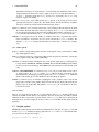
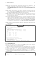
3.1 Input parameters
The n-way frequency table to be analyzed is described in SAS/IML by four arrays, called levels
(table dimensions), table (table frequencies), vnames (variable names), and lnames (variable
labels), shown in lines 6–11 below. These arrays are specified in the run mosaic statement (line
18) A great many options, all of which have default values, are specified by global variables in the
PROC IML step (e.g., lines 14–15) Hence, the program is typically used as follows:
1
2
3
4
5
6
7
8
9
10
11
libname mosaic ’˜/sasuser/mosaics’;
proc iml worksize=10000 symsize=10000;
reset storage=mosaic.mosaic;
load module=_all_;
*-- specify data table;
levels = { 2 2 2 };
*-- variable levels;
table = { ... };
*-- contingency table;
vnames = { Gender Admit Faculty}; *-- variable names;
lnames = { Male Female,
Yes No,
Arts Science};
12
13
14
15
16
*-- specify non-default global inputs;
fittype=’USER’;
config = { 1 1,
2 3 };
17
18
run mosaic(levels, table, vnames, lnames, plots, title);
The n-way contingency table to be analyzed is specified by the table parameter; the names of
the dimension (factor) variables and the names of the values that the dimension variables take on are
specified in the vnames and lnames parameters, respectively, as described below.
In situations where the contingency table and factor variables are available in a SAS dataset, the
table, levels, and lnames matrices may be constructed with the readtab module, described
in Section 3.5, “Dataset Input” The parameters for the run mosaic statement are:
Parameter Description
levels is a numeric vector which specifies the number of variables and the dimensions of the
contingency table. If levels is n × 1, then the table has n dimensions, and the number of
levels of variable i is levels[i]. The order of the variables in levels is the order they are
entered into the mosaic display.
table is a matrix or vector giving the frequency, fij... , of observations in each cell of the table.
The table variables are arranged in accordance with the conventions of the SAS/IML IPF and
MARG functions, so the first variable varies most rapidly across the columns of table and the
last variable varies most slowly down the rows. The table must be complete. If you use PROC
FREQ to sum a larger data set, use the SPARSE option on the TABLES statement so that all
combinations are created.
In addition table must conform to levels as follows. If table is I rows by J columns,
the product of all entries in levels must be IJ. Moreover, J must equal the product of the
first k entries of levels, for some k. That is, the columns must correspond to the combinations of one or more of the first k factors.
vnames is a 1×n character vector of variable (factor) names, in an order corresponding to levels.
lnames is a character matrix of labels for the variable levels, one row for each variable. The
number of columns is the maximum value in levels. When the number of levels are unequal,
the rows for smaller factors must be padded with blank entries.
3 USING MOSAICS
6
plots is a vector containing any of the integers 1 to n which specifies the list of marginal tables
to be plotted. If plots contains the value i the marginal subtable for variables 1 to i will be
displayed. For a 3-way table, plots={1 2 3} displays each sequential plot, showing the
[A], [AB] and [ABC] marginal tables; while plots=3 displays only the final 3-way [ABC]
mosaic.
title is a character string or vector of strings containing title(s) for the plots. If title is a single
character string, it is used as the title for all plots. Otherwise, title may be a vector of up to
max(plots) strings, and title[i] is used as the tile for the plot produced by plots[] =
i. If the number of strings is less than max(plots) the last string is used for all remaining
plots.
Moreover, if the title for a given plot contains the string &MODEL (upper case), that string is
replaced by the symbolic model description. Similarly, the string &G2 (or &X2) is replaced by
the LR (Pearson) chisquare value and df for the current model, in the form ’G2 (df) = value’.
Enclose such titles in single quotes; otherwise the SAS macro processor will complain about
an ’Apparent symbolic reference’. For example, the specifications,
plots = 2:3;
fittype=’JOINT’;
title = { ’’,
’Hair-color Eye-color Data
’Hair-color Eye-color Data
Model (H)(E)’,
Model (HE)(S)’};
produces two plots with titles from title[2] and title[3].1 Equivalent results (using
substitution) are produced with the single title,
title = ’Hair-color Eye-color Data
Model &MODEL’;
3.2 Global input variables
The global variables below allow many of the details of the model fitting and mosaic display to be
altered. Since they all have default values, it is only necessary to specify those you wish to change.
All character-valued variables are case-insensitive.
3.2.1 Analysis options
config is a numeric or character matrix specifying which marginal totals to fit when fittype=’USER’
is also specified. config is ignored for all other fit types. Each column specifies a high-order
marginal in the model, either by the names of the variables, or by their indices, according to
their order in vnames. For example, the log-linear model [AB][AC][BC] for a three-way
table is specified by the 2 by 3 matrix,
config = { 1
2
1
3
2,
3};
A
C
B,
C};
or
config = { A
B
The same model can be specified more easily row-wise, and then transposed:
config = t( {1 2, 1 3, 2 3} );
1 Some SAS/GRAPH fonts do not produce brackets,
formulae.
[ ] and braces, { }. Use parentheses instead in model symbolic
3 USING MOSAICS
7
devtype {GF |LR |FT [ADJ }] is a character string which specifies the type of deviations (residuals) to be represented by shading. devtype=’GF’ is the default.
p
GF calculates components of Pearson goodness of fit chisquare, d ij = (fij − m̂ij )/ m̂ij ,
where m̂ij is the estimated expected frequency under the model.
LR calculates components of the likelihood ratio (deviance) chisquare, d ij = sign(fij −
m̂ij )[2|fij log(fij /m̂ij )| + (fij − m̂ij )]1/2 .
p
p
p
FT calculates Freeman-Tukey residuals, dij = fij + fij + 1 − 4m̂ij + 1
√
ADJ Appending ADJ to one of the above options causes adjusted residuals ( = d/ 1 − h,
where h is the diagonal element of the “hat” matrix) to be calculated. Because 0 < h < 1,
the adjusted residuals are always larger in magnitude than the unadjusted values, however,
adjusted residuals have the property that their standard errors are equal, so their values
are more comparable over cells in the contingency table.
Adjusted residuals require additional computation (it becomes necessary to construct the
design matrix, X, and then calculate (X T W X)−1 ), however, experience shows that
they provide better visual display of the patterns of association than do ordinary Pearson
or LR residuals.
Table 1: Log-linear
MOSAICS.
fittypea
MUTUAL
JOINT
JOINT1
CONDIT
CONDIT1
PARTIAL
MARKOV1
MARKOV2
a
b
models corresponding to the various fittype values recognized by
3-wayb
4-way
5-way
[A] [B] [C]
[AB] [C]
[A] [BC]
[AC] [BC]
[AB] [AC]
[AC] [BC]
[AB] [BC]
[A] [B] [C]
[A] [B] [C] [D]
[ABC] [D]
[A] [BCD]
[AD] [BD] [CD]
[AB] [AC] [AD]
[ACD] [BCD]
[AB] [BC] [CD]
[ABC] [BCD]
[A] [B] [C] [D] [E]
[ABCE] [E]
[A] [BCDE]
[AE] [BE] [CE] [DE]
[AB] [AC] [AD] [AE]
[ADE] [BDE] [CDE]
[AB] [BC] [CD] [DE]
[ABC] [BCD] [CDE]
In all cases, the model [A] [B] is fit to a two-way table or marginal table.
The letters A, B, C, . . . refer to the table variables in the order of entry into the mosaic
display.
fittype {JOINT |MUTUAL |CONDIT |PARTIAL |MARKOV |USER} is a character string which
specifies the type of sequential log-linear models to fit. fittype=’JOINT’ is the default.
For two-way tables, (or two-way margins of larger tables) all fittypes fit the independence
model. The fittype values and the models they imply for (sub-)tables of various size are
summarized in Table 1.
JOINTk specifies sequential models of joint independence, [A][B], [AB][C], [ABC][D], ...
These models specify that the last variable in a given plot is independent of all previous
variables jointly.
Optionally, the keyword JOINT may be followed by a digit, k, to specify which of the n
ordered variables is independent of the rest jointly. e.g., JOINT1 gives [A][BC], . . ..
MUTUAL specifies sequential models of mutual independence, [A][B], [A][B][C], [A][B][C][D],
...
CONDITk specifies sequential models of conditional independence which hypothesize that all
previous variables are independent, given the last, i.e., [A][B], [AC][BC], [AD][BD][CD],
... For the 3-way model, A and B are hypothesized to be conditionally independent, given
C; for the 4-way model, A, B, and C are conditionally independent, given D.
3 USING MOSAICS
8
Optionally, the keyword CONDIT may be followed by a digit, k, to specify which of the
n ordered variables is conditioned upon.
PARTIAL specifies sequential models of partial independence of the first pair of variables,
conditioning on all remaining variables one at a time: [A][B], [AC][BC], [ACD][BCD],
... For the 3-way model, A and B are hypothesized to be conditionally independent, given
C; for the 4-way model, A and B are conditionally independent, given C and D.
MARKOVk specifies a sequential series of Markov chain models fit to the table, whose dimensions are assumed to represent discrete ordered time points, such as lags in a sequential analysis. The keyword MARKOV can be optionally followed by a digit to specify
the order of the Markov chains, e.g., fittype=’MARKOV2’; specifies a second-order
Markov chain. First-order is assumed if not specified. Such models assume that the table
dimensions are ordered in time, e.g., Lag0, Lag1, Lag2, ...
MARKOV (or MARKOV1) fits the models [A][B], [AB][BC], [AB][BC][CD], ... where
the categories at each lag are associated only with those at the previous lag. MARKOV2
fits the models [A][B], [A][B][C], [ABC][BCD], [ABC][BCD][CDE], ...
USER If fittype=’USER’, specify the hypothesized model in the global matrix config.
The models for plots of marginal tables are based on reducing the hypothesized configuration, eliminating all variables not participating in the current plot.
order {NONE |[ DEV |JOINT ] |[ ROW |COL ] } Specifies whether and how to perform a correspondence analysis to assist in reordering the levels of each factor variable as it is entered into
the mosaic display. Not performed if order=’NONE’. Otherwise, order may be a character
vector containing either ’DEV’ or ’JOINT’ to specify that the CA is performed on residuals
from the model for the current subtable (DEV) or on residuals from the model of joint independence for this subtable (JOINT). In addition, order may contain either ’ROW’ or ’COL’
or both to specify which dimensions of the current subtable are considered for reordering. The
usual options for this reordering are
order = {JOINT COL};
At present this analysis merely produces printed output which suggests an ordering, but does
not actually reorder the table or the mosaic display.
zeros is a matrix of the same size and shape as the input table containing entries of 0 or 1,
where 0 indicates that the corresponding value in table is to be ignored or treated as missing or
a structural zero.
Zero entries cause the corresponding cell frequency to be fitted exactly; one degree of freedom
is subtracted for each such zero. The corresponding tile in the mosaic display is outlined in
black.
If an entry in any marginal subtable in the order [A], [AB], [ABC] ... corresponds to an allzero margin, that cell is treated similarly as a structural zero in the model for the corresponding
subtable. Note, however, that tables with zero margins may not always have estimable models.
If the table contains zero frequencies which should be treated as structural zeros, assign the
zeros matrix like this:
zeros = table > 0;
For a square table, to fit a model of quasi-independence ignoring the diagonal entries, assign
the zeros matrix like this (assuming a 4 × 4 table):
zeros = J(4,4) - I(4);
3 USING MOSAICS
9
3.2.2 Display options
abbrev If abbrev> 0, variable names are abbreviated to that many letters in the model formula
(and in the plot title if title=’&MODEL’).
cellfill {NONE |SIGN |SIZE |DEV |FREQ} min Provides the ability to display a symbol in
the cell representing the coded value of large residuals. This is particularly useful for black and
white output, where it is difficult to portray both sign and magnitude distinctly.
NONE Nothing (default)
SIGN Draws + or − symbols in the cell, whose number corresponds to the shading density.
SIZE Draws + or − symbols in the cell, whose size corresponds to the shading density.
DEV Writes the value of the standardized residual in the cell, using format 6.1.
FREQ Writes the value of the cell frequency in the cell, using format 6.0.
If a numeric value, min is also specified (e.g., cellfill=’DEV 2’), then only cells whose
residual exceeds that value in magnitude are so identified.
colors is a character vector of one or two elements specifying the colors used for positive and negative residuals. The default is {BLUE RED}. For a monochrome display, specify colors=’BLACK’
and use two distinct fill patterns for the fill type, such as filltype={M0 M45} or filltype={GRAY
M45}.
filltype {M45 |LR |M0 |GRAY |HLS} is a character vector of one or two elements which
specifies the type of fill pattern to use for shading. filltype[1] is used for positive residuals; filltype[2], if present, is used for negative residuals. If only one value is specified, a
complementary value for negative residuals is generated internally. filltype={HLS HLS}
is the default, which usually looks best for color output.
M45 uses SAS/GRAPH patterns MdN135 and Md45 with hatching at 45 and 135◦ . d is the
density value determined from the residual and the shade parameter.
LR uses SAS/GRAPH patterns Ld and Rd.
M0 uses SAS/GRAPH patterns MdN0 and MdN90 with hatching at 0 and 90◦ .
GRAYstep uses solid, greyscale fill using the patterns GRAYnn starting from GRAYF0 for
density=1 and increasing darkness by step for each successive density level. The default
for step is 16, so ’GRAY’ gives GRAYF0, GRAYE0, GRAYD0, and so forth.
HLS uses solid, color-varying fill based on the HLS color scheme. The colors are selected attempting to vary the lightness in approximately equal steps. For this option, the colors
values must be selected from the following hue names: RED GREEN BLUE MAGENTA
CYAN YELLOW.
fuzz is a numeric value which specifies the smallest absolute residual to be considered equal to
zero. Cells with |dij | < fuzz are outlined in black. The default is fuzz = 0.20.
htext is a numeric value which specifies the height of text labels, in character cells. The default is
htext=1.3. The program attempts to avoid overlap of category labels, but this cannot always
be achieved. Adjust htext (or make the labels shorter) if they collide.
legend {H |V |NONE} Orientation of legend for shading of residual values in mosaic tiles. ’V’
specifies a vertical legend at the right of the display; ’H’ specifies a horizontal legend beneath
the display. Default: ’NONE’.
shade is a vector of up to 5 values of |dij |, which specify the boundaries between shading levels.
If shade={2 4} (the default), then the shading density number d is:
d
0
1
2
residuals
0 ≤ |dij | < 2
2 ≤ |dij | < 4
4 ≤ |dij |
3 USING MOSAICS
10
Standardized deviations are often referred to a standard Gaussian distribution; under the assumption that the model fits, these values roughly correspond to two-tailed probabilities p <
.05 and p < .0001 that a given value of |dij | exceeds 2 or 4, respectively. Use shade= a big
number to suppress all shading.
space is a vector of two values which specify the x, y percent of the plotting area reserved for
spacing between the tiles of the mosaic. The default value is 10 times the number of variables
allocated to each of the vertical and horizontal directions in the plot.
split is a character vector consisting of the letters V and H which specifies the directions in which
the variables divide the unit square of the mosaic display. If split={H V} (the default), the
mosaic alternates between horizontal and vertical splitting. If the number of elements in split
is less than the maximum number in plots, the elements in split are reused cyclically.
vlabels is an integer from 0 to the number of variables in the table. It specifies that variable
names (in addition to level names) are to be used to label the first vlabels variables. The
default is vlabels=2, meaning variable names are used in plots of the first two variables
only.
3.2.3 Other options
gout is a character string which specifies the name of the graphics catalog. The default is GSEG
(the default graphics catalog).
name is a character string (up to 7 characters) which specifies the prefix for the names of the graphs
in the graphics catalog. The default is MOSAIC.
outstat is a character string containing the name of an optional output data set containing the following variables: RESIDUAL, FITTED, and FREQ. The variable FACTORS gives the number
of factors in a given mosaic display, and LABELS gives the cell labels for each cell in the given
table.
verbose {NONE |FIT |BOX} is a character vector of one or more words which controls verbose
or detailed output. If verbose contains ’FIT’, additional details of the fitting process
(fitted frequencies, marginal proportions) are printed. If verbose contains ’BOX’, additional
details of the drawing process (tile dimensions, label placement) are printed.
window is a numeric vector of 4 elements containing the world coordinates of the lower left and
upper right coordinates of the graphics window used for the mosaic display. The actual mosaic
fills the region {0, 0, 100, 100}. The default window is set to {-16 -16, 108 108} to allow for
text labels and a title.
3.2.4 Caveats
There is one caveat imposed by this use of global variables: The mosaic module should not be
called from an IML module with its own arguments, since this would cause all variables defined
within that module to inaccessible as global variables. The mosaic module may be called either in
immediate mode, as in the example in secrefsec:ex-direct, or from an IML module defined without
arguments.
3.3 Graphic options
MOSAICS assumes that the vertical and horizontal dimensions of the plot are equal, so you should
include a goptions statement specifying equal values for hsize and vsize if the default values
for your device are unequal. For example,
goptions hsize=7 in vsize=7 in;
3 USING MOSAICS
11
By default, the program uses shades of the colors blue and red to draw the tiles corresponding
to positive and negative residuals. It cannot respect the global colors= options on the goptions
statement. You can specify the IML global colors variable to change these assignments if you
wish. (Or, change the default values in the globals module.)
The program cannot access global fonts assigned with the GOPTIONS FTEXT= and HTEXT=
options. Instead, you may specify a desired font with the IML global font and htext variables. For
some output devices (e.g., PostScript), specifying a hardware font (e.g., font = ’hwpsl009’;
for Helvetica) can yield an enormous reduction in the size of the generated graphic output files. By
default, the program uses the Helvetica hardware font when it detects a PostScript device, and uses
the SWISS font otherwise.
3.3.1 EPS Output
Some output devices, such as Encapsulated Postscript (and GIF) require that each figure be written to
a separate output file. Mosaics contains a gskip module which handles this automatically for EPS
output.
It uses three global SAS macro variables:
DEVTYP Device type: Use %let devtyp=eps; for EPS output. Ordinarily, %let devtyp=screen;
for Display Manager
DISPLAY Display option: Use %let display=ON; for ordinary use. Setting DISPLAY=OFF
suppresses graphic output (for all devices).
FIG Figure number: Initialize to 1 %let fig=1;
Listed below is a macro, EPS, which I use to initialize graphics options for EPS output.
%global fig gsasfile devtyp;
%macro eps;
%let devtyp = EPS;
%let fig=1;
%let gsasfile=grfout.eps;
%put gsasfile is: "&gsasfile";
filename gsasfile "&gsasfile";
goptions horigin=.5in vorigin=.5in; *-- override, for BBfix;
goptions device=PSLEPSFC gaccess=gsasfile
gend=’0A’x gepilog=’showpage’ ’0A’x
/* only for 6.07 */
gsflen=80 gsfmode=replace;
%mend;
3.4 Multiple calls
The mosaic module may be called repeatedly in one PROC IML step. However, global variables
which are set in one call remain in force. To restore these values to their default setting, use the
SAS/IML free statement. For example, to revert to the default fit type of joint independence, use
the statement,
free fittype;
before the next run mosaic statement.
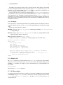
3.5 SAS Dataset Input
A contingency table and its index (factor) variables may be read into SAS/IML in the format required
for MOSAICS using the readtab module, as shown in the following example. The factors in the
2 × 3 × 2 table are gender, occup, and heart. The dataset heart has 12 observations—one
observation per cell.
3 USING MOSAICS
1
2
3
4
5
6
7
8
9
10
11
12
13
14
15
12
karger.sas
* Sex, Occupation and heart disease [Karger, 1980];
data heart;
input gender $ occup $ @;
heart=’Disease’; input freq @; output;
heart=’No Dis’;
input freq @; output;
cards;
Male
WhiteCol
158
3155
Female WhiteCol
52
3082
Male
BlueCol
87
2829
Female BlueCol
16
416
Male
Unempl
254
759
Female Unempl
431 10283
;
proc sort data=heart;
by heart occup gender;
16
17
18
19
20
proc iml worksize=10000 symsize=10000;
title = ’Sex, Occupation, and Heart Disease’;
reset storage=mosaic.mosaic;
load module=_all_;
21
22
23
vnames = {’Gender’ ’Occup’ ’Heart’ };
run readtab(’heart’, ’freq’, vnames, table, levels, lnames);
24
25
26
plots = 2:ncol(levels);
run mosaic(levels, table, vnames, lnames, plots, title);
The readtab routine reads the index (factor) variables from the input dataset (heart), and determines the order of the factor variables according to which variable is actually varying most rapidly in
the input dataset. The variable names vector (vnames) can be given in any order; it is reordered to
correspond to the order of observations in the input dataset.
Note that if you sort the dataset as in the example above, character-valued index variables are arranged in alphabetical order. For example, the levels of occup are arranged in the order BlueCol,
Unempl, WhiteCol, which may or may not be what you want. The PROC SORT step can be
omitted, in which case the levels are ordered according to their order in the input dataset.
You can also use the DESCENDING option in the PROC SORT step to reverse the order of the
levels of a given factor. For example, to reverse the levels of the gender variable, use
proc sort data=heart;
by heart occup descending gender;
3.6 Fitting specialized models
For square tables, or tables with ordered factors, a wide variety of specialized models are available
which cannot be specified as any IPF configuration for a hierarchical loglinear model. However, many
of these models can be fit simply using the matrix operations and functions available in SAS/IML.
For example, the model of symmetry for a square table has expected frequencies m̂ ij = (fij +
fji )/2. The fitted frequencies and residuals can be calculated in SAS/IML as
fit = (f + f‘)/2;
dev = (f - fit)/sqrt(fit);
where f is a square table of observed frequencies.
4 MACRO INTERFACE
13
MOSAICS includes an additional program, mosaicd.sas, designed for situations such as this,
where the fitted values and residuals are calculated externally (e.g., with IML programming statements or with PROC CATMOD or PROC GENMOD). The mosaicd is then called instead of mosaic.
The residuals are supplied as a dev parameter (which replaces the plots parameter of mosaic).
The following example uses mosaicd to fit a model of symmetry to a 4 × 4 table of women
classified by visual acuity ratings of their left and right eyes.
1
2
3
4
5
6
7
8
9
10
11
12
13
14
15
16
17
18
proc iml worksize=10000 symsize=10000;
dim = { 4 4 };
/* Unaided distant vision data Bishop etal p. 284*/
/*
Left eye grade */
f = {1520
266
124
66,
234 1512
432
78,
117
362 1772
205,
36
82
179
492 };
title = {’Unaided distant vision: Symmetry’};
vnames = {’Right Eye’,’Left Eye’};
lnames = { ’High’ ’2’ ’3’ ’Low’,
’High’ ’2’ ’3’ ’Low’};
reset storage=mosaic.mosaic;
load module=_all_;
%include ’˜/sasuser/mosaics/mosaicd.sas’;
fit = (f + f‘)/2;
dev = (f - fit)/sqrt(fit);
run mosaicd(dim, f, vnames, lnames, dev, title);
The sample program, moseye.sas, included in the distribution archives, illustrates how models of
quasi-independence and quasi-symmetry can also be fit with MOSAICS.
4
Macro interface
4.1 The MOSAIC macro
The MOSAIC macro provides an easily used macro interface to the MOSAICS and MOSAICD
SAS/IML programs. Using the SAS/IML programs directly means that you must compose a proc
iml step and invoke the mosaic module, as described in Section 3.1.
The MOSAIC macro may be used with any SAS dataset in frequency form (e.g., the output
from PROC FREQ). The macro simply creates the proc iml step, reads the input dataset(see Section 3.5), and runs the mosaic module.
If your data is in case form, or you wish to collapse over some table variables, you must use PROC
FREQ) first to construct the contingency table to be analyzed. The TABLE macro may be used for
this purpose. It has the advantage of allowing formatted values of the table factors to be used by the
mosaics program.
Ordinarily, the program fits a model (specified by the fittype= parameter) and displays residuals from this model in the mosaic for each marginal subtable specified by the PLOTS= parameter.
However, if you have already fit a model and calculated residuals some other way (e.g., using PROC
CATMOD or PROC GENMOD), specify a RESID= variable in the macro call. The macro will then call
the mosaicd module, as described in Section 3.6.
The MOSAIC macro is easier to use, but is not as flexible as direct use of the SAS/IML programs.
• Factor levels are labelled using the values of the factor variables in the input dataset. You
cannot simply attach a SAS format to a factor to convert numeric values to character labels, but
you can use a DATA step to create character equivalents of numeric variables using the put()
function, or use the TABLE macro.
4 MACRO INTERFACE
14
• You cannot reorder the factors, or the levels of a factor as flexibly as you can in SAS/IML. If
you use the SORT= parameter, take care that an ordered factor (‘Low’, ‘Medium’, ’High’) is
not sorted alphabetically.
Usage
The mosaic macro is called with the keyword parameters below. Either the VAR= or the VORDER=
parameter is required.
%mosaic(
data=_last_,
var=,
count=count,
by=,
fittype=joint,
config=,
devtype=gf,
shade=2 4,
plots=,
colors=blue red,
fill=HLS HLS,
split=V H,
vorder=,
htext=1.5,
font=,
title=,
space=,
cellfill=,
vlabels=,
sort=,
resid=,
fuzz=,
order=,
lorder=,
legend=,
outstat=,
zeros=,
name=mosaic,
gout=
);
/*
/*
/*
/*
/*
/*
/*
/*
/*
/*
/*
/*
/*
/*
/*
/*
/*
/*
/*
/*
/*
/*
/*
/*
/*
/*
/*
/*
/*
Name of input dataset
Names of all factor variable
Name of the frequency variable
Name(s) of BY variables
Type of models to fit
User model for fittype=’USER’
Residual type
shading levels for residuals
which plots to produce
colors for + and - residuals
fill type for + and - residuals
split directions
order of variables in mosaic
height of text labels
font for text labels
title for plot(s)
room for spacing the tiles
write residual in the cell?
Number of variable names used as plot labels
Pre-sort variables?
Name of residual variable
Fuzz value for residuals near 0
Do CA on marginal tables?
Reorder levels of one or more variables
Legend for shading levels: H, V or NONE
Name of an output data set of fit statistics
0/1 variable, where 0 indicates structural 0
base name of graphic catalog entries
name of graphic catalog
*/
*/
*/
*/
*/
*/
*/
*/
*/
*/
*/
*/
*/
*/
*/
*/
*/
*/
*/
*/
*/
*/
*/
*/
*/
*/
*/
*/
*/
The parameters for the mosaic macro are like those of the SAS/IML program (see Section 3.1),
except:
data= Specifies the name of the input dataset. Should contain one observation per cell, the variables
listed in VAR= and COUNT=, and possibly RESID= and BY=. .
var= Specifies the names of the factor variables for the contingency table. Abbreviated variable lists
are not allowed. The levels of the factor variables may be character or numeric, but are used ‘as
is’ in the input data. That is, a numeric variable with an attached user-defined format appears
as numeric. You may omit the VAR= variables if variable names are used in the VORDER=
parameter.
by= Specifies the names of one (or more) By variables. Partial mosaic plots are produced for each
combination of the levels of the BY= variables. The BY= variable(s) must be listed among the
VAR= variables.
count= Specifies the names of the frequency variable in the dataset
4 MACRO INTERFACE
15
config= For a user-specified model, config gives the terms in the model, separated by ’/’. For
example, to fit the model of no-three-way association, specify config=1 2 / 1 3 / 2
3, or (using variable names) config = A B / A C / B C. Note that the numbers refer
to the variables after they have been reordered, either sorting the data set, or by the vorder=
parameter.
vorder= Specifies either the names of the variables or their indices in the desired order in the
mosaic. Note that using the VORDER parameter keeps the factor levels in their order in the
data, whereas the SORT parameter arranges factor levels in sorted order.
lorder= Specifies a reordering of the levels of one or more variables, of the form ’A: a2 a1 a3 /
B: b2 b3 b4 b1’, where ’/’ separates different variables and ’:’ separates the name of a variable
from the desired order of the levels.
sort= Specifies whether and how the input data set is to be sorted to produce the desired order of
variables in the mosaic. SORT=YES sorts the data in the reverse order that they are listed in the
VAR= paraemter, so that the variables are entered in the order given in the VAR= parameter.
Otherwise, SORT= lists the variable names, possibly with the DESENDING or NOTSORTED
options in the reverse of the desired order. e.g., SORT=C DESCENDING B DESCENDING A
resid= Specifies that externally calculated residuals are contained in the variable named by the
resid= parameter.
Here is an example:
1
2
3
4
5
6
7
8
9
10
11
12
13
14
15
16
17
druguse.sas
title ’Alcohol, Cigarette, and Marijuana Use by High School Seniors’;
* Source: Agresti, 1996, p. 152;
data druguse;
input alcohol $ cigaret $ @;
marijuan = ’Mar:+’; input freq @; output;
marijuan = ’Mar:- ’; input freq @; output;
cards;
Alc:+ Cig:+
911
538
Alc:+ Cig:44
456
Alc:- Cig:+
3
43
Alc:- Cig:2
279
;
goptions hsize=7in vsize=7in;
%mosaic(var=alcohol cigaret marijuan,
count=freq, plots=2:3,
fittype=condit,
title=%str(Alcohol, Cigarette, and Marijuana Use));
4.2 The MOSMAT macro
The MOSMAT macro uses the MOSAICS and MOSMAT SAS/IML programs to create a scatterplot
matrix of mosaic displays for all pairs of categorical variables.
Each pairwise plot shows the marginal frequencies to the order specified by the PLOTS= parameter. When PLOTS=2, these are the bivariate margins, and the residuals from marginal independence
are shown by shading. When PLOTS>2, the observed frequencies in a higher-order marginal table
are displayed, and the model fit to that marginal table is determined by the FITTYPE= parameter.
The keyword parameters and their default values are listed below. Either the VAR= or the VORDER=
parameter is required.
%macro mosmat(
data=_last_,
var=,
/* Name of input dataset
/* Names of factor variables
*/
*/
5 EXAMPLES
count=count,
fittype=joint,
config=,
devtype=gf,
shade=,
plots=2,
colors=blue red,
fill=HLS HLS,
split=V H,
vorder=,
htext=,
font=,
title=,
space=,
fuzz=,
abbrev=,
sort=YES,
);
16
/*
/*
/*
/*
/*
/*
/*
/*
/*
/*
/*
/*
/*
/*
/*
/*
/*
Name of the frequency variable
Type of models to fit
User model for fittype=’USER’
Residual type
shading levels for residuals
which plots to produce
colors for + and - residuals
fill type for + and - residuals
split directions
order of variables in mosaic
height of text labels
font for text labels
title for plot(s)
room for spacing the tiles
smallest abs resid treated as zero
abbreviate variable names in model
Sort variables first?
*/
*/
*/
*/
*/
*/
*/
*/
*/
*/
*/
*/
*/
*/
*/
*/
*/
4.3 The TABLE macro
The TABLE macro constructs a grouped frequency table suitable for input to the MOSAIC macro or
the MOSMAT macro. The input data may be individual observations, or a contingency table, which
may be collapsed to fewer variables. Factor variables may be converted to character using usersupplied formats.
See Section 5.4 for an example.
%macro table (
data=_last_,
var=,
char=,
weight=,
order=,
format=,
out=table
);
5
/*
/*
/*
/*
/*
/*
/*
Name of input dataset
Names of all factor variables
Force factor variables to character?
Name of a frequency variable
Specifies the order of the variable levels
List of var, format pairs
Name of output dataset
*/
*/
*/
*/
*/
*/
*/
Examples
The examples below were written sequentially as the MOSAICS package developed, so the initial
examples (Section 5.1–Section 5.3) illustrates its use within SAS/IML. The macro interface was
developed later, and PROC GENMOD now allows a wider class of models to be fit than could be
handled by the IPF algorithm in SAS/IML. Readers who wish to avoid SAS/IML should start with
the example in Section 4.1 and Section 5.5.
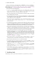
5.1 Example 1: Direct use in IML
The program below shows the use of MOSAICS to produce a set of different mosaic displays for a
4 × 4 × 2 table of 592 people classified by hair color, eye color and sex.
The module haireye creates the variables table, levels, vnames, lnames, and title.
Since the variables are to be entered into the mosaic in the order hair color, eye color, and sex, the
table variable is created as a 2 × 16 matrix with hair color varying most rapidly across the columns
and sex varying down the two rows. Note that the lnames variable is a 3 × 4 matrix, and the last row
contains two blank values. The statement run haireye; creates these variables in the SAS/IML
workspace.
5 EXAMPLES
17
Standardized
residuals:
Brown
<-4
-4:-2 -2:-0 0:2
2:4
Hazel GreenBlue
>4
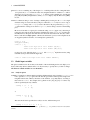
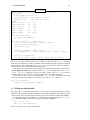
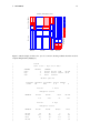
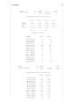
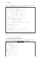
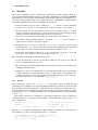
The first run mosaics statement produces two plots, whose tiles show the [Hair][Eye] marginal
table and the full three-way table. Since fittype is not specified, the model [HairEye] [Sex], in
which Sex is independent of hair color and eye color jointly, is fit to the three-way table. split={V
H} specifies that the first division of the mosaic is in the vertical direction. The printed output produced from this run is shown below.
Black
Brown
Red
Blond
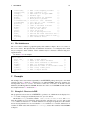
Figure 1: Two-way mosaic for hair color and eye color. Positive deviations from independence have
solid outlines and are shaded blue. Negative deviations have dashed outlines and are shaded red. The
two levels of shading density correspond to standardized deviations greater than 2 and 4 in absolute
value.
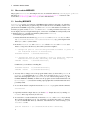
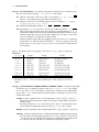
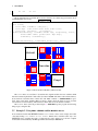
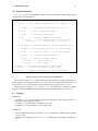
The second run mosaics statement (line 33) fits the same models, but reorders the eye colors
in the table to better display the pattern of association between hair color and eye color in the two-way
table. It is also necessary to rearrange the eye color labels in row 2 of lnames. (This reordering is
based on a correspondence analysis of residuals in the two-way table, as described in [3] carried out
separately. See the order global variable in Section 3.2.) Note that the global variables split and
htext specified in the first mosaic continue to be used here. The plots produced from this call are
shown in Figure 1 and Figure 2.
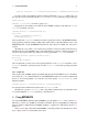
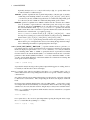
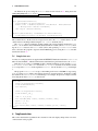
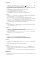
The third run mosaics statement (line 37) plots only the three-way display, showing residuals
from the model in which hair color, eye color and sex are mutually independent. This plot is shown
in Figure 3.
1
goptions vsize=7in hsize=7in ;
mosademo.sas
*-- square plot environment;
2
3
4
5
6
7
8
9
proc iml worksize=10000 symsize=10000;
start haireye;
*-- Hair color, eye color data;
table = {
/* ----brown-------blue--------hazel--32 53 10 3
11 50 10 30
10 25 7 5
36 66 16 4
9 34
7 64
5 29 7 5
---green--- */
3 15 7 8,
/*M*/
2 14 7 8 }; /*F*/
10
11
12
13
levels= { 4 4 2 };
vnames = {’Hair’ ’Eye’ ’Sex’ };
lnames = {
/* Variable names */
/* Category names */
5 EXAMPLES
18
Male Female
Black
Standardized
residuals:
Brown
<-4
-4:-2 -2:-0 0:2
2:4
Hazel GreenBlue
>4
Model (HairEye)(Sex)
Brown
Red
Blond
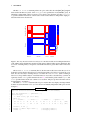
Figure 2: Mosaic display for hair color, eye color, and sex. The categories of sex are crossed with
those of hair color, but only the first occurrence is labeled. Residuals from the model [HE] [S] are
shown by shading.
14
15
16
17
18
’Black’ ’Brown’ ’Red’ ’Blond’,
’Brown’ ’Blue’ ’Hazel’ ’Green’,
’Male’ ’Female’ ’ ’ ’ ’ };
title = ’Hair color - Eye color data’;
finish;
/* hair color */
/* eye color */
/* sex
*/
19
20
21
22
23
24
25
26
27
run haireye;
reset storage=mosaic.mosaic;
load module=_all_;
*-- Fit models of joint independence (fittype=’JOINT’);
plots = 2:3;
split={V H};
htext=1.6;
run mosaic(levels, table, vnames, lnames, plots, title);
28
29
30
31
32
33
*-- reorder eye colors (brown, hazel, green, blue);
table = table[,((1:4) || (9:16) || (5:8))];
lnames[2,] = lnames[2,{1 3 4 2}];
plots=2:3;
run mosaic(levels, table, vnames, lnames, plots, title);
34
35
36
37
38
plots=3;
fittype=’MUTUAL’;
run mosaic(levels, table, vnames, lnames, plots, title);
quit;
+-----------------------------------------------------------------+
|
+-------------------------------------------+
|
|
|Generalized Mosaic Display, Version 2.9
|
|
|
+-------------------------------------------+
|
|
|
5 EXAMPLES
19
Standardized
residuals:
Brown
<-4
-4:-2 -2:-0 0:2
2:4
Hazel GreenBlue
>4
Model (Hair)(Eye)(Sex)
MaleFemale
Black
Brown
Red
Blond
Figure 3: Mosaic display for hair color, eye color, and sex, showing residuals from the model of
complete independence, [H] [E] [S]
|
|
|
|
|
|
|
|
|
|
|
|
|
|
|
|
|
|
|
|
|
|
|
|
|
|
|
|
|
|
|
|
TITLE
Hair color - Eye color data
VNAMES
Hair
Eye
Sex
LEVELS
4
4
2
LNAMES
Black Brown Red
Brown Hazel Green
Male
Female
Blond
Blue
Global options
FITTYPE
JOINT
DEVTYPE
GF
FILLTYPE
M45
Factor:
SPLIT
V H
SHADE
2
4
1 Hair
Marginal totals
MARGIN
Black
Brown
Red
Blond
108
286
71
127
Factor:
2 Eye
Marginal totals
MARGIN
Black
Brown
Red
Blond
Brown
Hazel
Green
Blue
68
119
26
7
15
54
14
10
5
29
14
16
20
84
17
94
|
|
|
|
|
|
|
|
|
|
|
|
|
|
|
|
|
|
|
|
|
|
|
|
|
|
|
|
|
|
|
|
5 EXAMPLES
|
|
|
|
|
|
|
|
|
|
|
|
|
|
|
|
|
|
|
|
|
|
|
|
|
|
|
|
|
|
|
|
|
|
|
|
|
|
|
|
|
|
|
|
|
|
|
|
|
|
|
|
|
|
|
|
|
|
|
|
20
MODEL
{Hair}{Eye}
DF
9
CHISQ
G.F.
L.R.
PROB
0.0000
0.0000
138.290
146.444
Standardized Pearson deviations
Black
Brown
Red
Blond
Brown
Hazel
Green
Blue
4.40
1.23
-0.07
-5.85
-0.48
1.35
0.85
-2.23
-1.95
-0.35
2.28
0.61
-3.07
-1.95
-1.73
7.05
Factor:
3 Sex
Marginal totals
MARGIN
Black
Black
Black
Black
Brown
Brown
Brown
Brown
Red
Red
Red
Red
Blond
Blond
Blond
Blond
Brown
Hazel
Green
Blue
Brown
Hazel
Green
Blue
Brown
Hazel
Green
Blue
Brown
Hazel
Green
Blue
MODEL
[Hair,Eye][Sex]
DF
15
Male
Female
32
10
3
11
38
25
15
50
10
7
7
10
3
5
8
30
36
5
2
9
81
29
14
34
16
7
7
7
4
5
8
64
CHISQ
G.F.
L.R.
28.993
29.350
Standardized Pearson deviations
Black
Black
Black
Black
Brown
Brown
Brown
Brown
Red
Red
Red
Red
Blond
Blond
Brown
Hazel
Green
Blue
Brown
Hazel
Green
Blue
Brown
Hazel
Green
Blue
Brown
Hazel
Male
Female
0.30
1.28
0.52
0.70
-2.07
0.19
0.57
2.05
-0.47
0.30
0.30
0.88
-0.07
0.26
-0.27
-1.15
-0.46
-0.63
1.86
-0.17
-0.52
-1.84
0.42
-0.27
-0.27
-0.79
0.06
-0.23
PROB
0.0161
0.0145
|
|
|
|
|
|
|
|
|
|
|
|
|
|
|
|
|
|
|
|
|
|
|
|
|
|
|
|
|
|
|
|
|
|
|
|
|
|
|
|
|
|
|
|
|
|
|
|
|
|
|
|
|
|
|
|
|
|
|
|
5 EXAMPLES
21
|
Blond Green
0.32
-0.29
|
|
Blond Blue
-1.84
1.65
|
|
|
+-----------------------------------------------------------------+
5.2 Example 2: PROC IML: Input from SAS data set
This example illustrates input of data from a SAS data set and the use of PROC SORT to rearrange
the variables in a table to the order desired in the mosaic displays.
The data is a 24 table classified by Gender, reported Pre-marital sex, Extra-marital sex and Marital
Status, read in by the DATA step marital below. Note that the variable marital varies most
rapidly and the variable gender varies most slowly in the observations in the data set. The desired
order of the variables in the mosaic is Gender, Pre, Extra, and Marital. In the table variable in
SAS/IML the first variable, Gender, must vary most rapidly. This is accomplished by sorting the
observations with the variables listed in the reverse order on the by statement in the PROC SORT
step.
1
2
3
4
5
6
7
8
9
10
11
12
13
14
15
16
data marital;
input gender $ pre $ extra $ @;
marital=’Divorced’; input freq @;
marital=’Married’;
input freq @;
cards;
Women Yes Yes
17
4
Women Yes No
54 25
Women No
Yes
36
4
Women No
No
214 322
Men
Yes Yes
28 11
Men
Yes No
60 42
Men
No
Yes
17
4
Men
No
No
68 130
;
proc sort data=marital;
by marital extra pre gender;
output;
output;
In the PROC IML step, the statement use marital; accesses the data set. The variable freq
from the data set is read into the IML table variable, a 16 × 1 matrix. Note that the levels of the
character variables gender, pre, and extra are sorted alphabetically, so the category labels in
lnames must appear in this order.
17
18
19
20
21
22
23
24
25
26
proc iml worksize=10000 symsize=10000;
use marital;
read all var{freq} into table;
levels = { 2 2 2 2 };
vnames = {’Gender’ ’Pre’ ’Extra’ ’Marital’};
lnames = {’Men
’ ’Women
’,
’Pre Sex: No’ ’Yes’,
’Extra Sex: No’
’Yes’,
’Divorced’
’Married’ };
title = ’Pre/Extramarital Sex and Marital Status’;
27
28
29
30
31
32
33
reset storage=mosaic.mosaic;
load module=_all_;
split = {V H};
htext=1.6;
plots = 2:4;
run mosaic(levels, table, vnames, lnames, plots, title);
5 EXAMPLES
22
34
35
36
37
38
39
40
41
plots = 4;
fittype=’USER’;
title =’Model (GPE, PM, EM)’;
config = { 1 2 3,
2 4 4,
3 0 0};
run mosaic(levels, table, vnames, lnames, plots, title);
The first run mosaic statement produces plots of the 2-way to 4-way tables, fitting models of
joint independence. The second run mosaic statement produces a plot of the 4-way table, fitting
the model [GPE] [PM] [EM] specified by the config variable and fittype=’USER’;. This
model treats G, P, and E as explanatory, and M as a response. This is equivalent to the logit model
with main effects of premarital sex and extramarital sex on marital status.
Using the readtab routine, this example can be simplified as follows. The routine constructs the
table, levels, and lnames variables. (But note that the values of the Pre and Extra variables
are both simply ’Yes’ or ’No’.)
1
2
3
4
proc iml worksize=10000 symsize=10000;
vnames = {’Gender’ ’Pre’ ’Extra’ ’Marital’};
run readtab(’marital’, ’freq’, vnames, table, levels, lnames);
title = ’Pre/Extramarital Sex and Marital Status’;
5
6
7
8
9
10
11
12
reset storage=mosaic.mosaic;
load module=_all_;
split = {V H};
htext=1.6;
plots = 2:4;
run mosaic(levels, table, vnames, lnames, plots, title);
...
5.3 Example 3: Reordering variables
This example shows the use of SAS/IML itself to reorder the variables in a contingency table for the
mosaic display. It uses the same data as in the previous example.
The variables in a contingency table are reordered by the MARG function (which calculates
marginal totals) when the model specified by the config parameter is the saturated model, with the
variables listed in the desired order. For example, for the four-way table of the previous example, the
configuration { 4,3,2,1 } gives the same order of the variables created by the PROC SORT step.
mosaics.sas includes an IML module transpos (shown partly below) which will reorder
the variables in any table. It also rearranges the values in the levels, vnames, and lnames
variables in the same order. The order parameter must be either a permutation of the integers
1:ncol(dim), or a permutation of the variable names in vnames.
start transpos(dim, table, vnames, lnames, order);
*-- reorder the dimensions of an n-way table;
if nrow(order) =1 then order=order‘;
run marg(loc,newtab,dim,table,order);
table = newtab;
dim = dim[order,];
vnames = vnames[order,];
lnames = lnames[order,];
finish;
The data table is defined, listing the observations in the same order as in the DATA step
marital shown in Example 2. Note that vnames and lnames conform to this order. After the
5 EXAMPLES
23
call to transpos the variables table, levels, vnames, and lnames have been rearranged
so that Gender is the first variable in the mosaic, and Marital status is last.
1
2
3
4
5
6
7
8
9
10
11
12
13
14
15
16
17
proc iml worksize=10000 symsize=10000;
*-- define the data variables;
table={ 17
4 , /* Women Yes Yes */
54 25 , /* Women Yes No
*/
36
4 , /* Women No
Yes */
214 322 , /* Women No
No
*/
28 11 , /* Men
Yes Yes */
60 42 , /* Men
Yes No
*/
17
4 , /* Men
No
Yes */
68 130 }; /* Men
No
No
*/
levels = { 2 2 2 2 };
vnames = {’Marital’ ’Extra’ ’Pre’ ’Gender’};
lnames = {’Divorced’
’Married’,
’Extra Sex: Yes’ ’No’,
’Pre Sex: Yes’
’No’,
’Women
’
’Men’ };
title = ’Pre/Extramarital Sex and Marital Status’;
18
19
20
reset storage=mosaic.mosaic;
load module=_all_;
21
22
23
24
25
26
27
ord = { 4,3,2,1};
run transpos(levels, table, vnames, lnames, ord);
split = {V H};
plots = 2:4;
run mosaic(levels, table, vnames, lnames, plots, title);
quit;
Note that the order of variables could also be specified using their names (case doesn’t matter) in line
23, as
ord = {gender pre extra marital};
5.4 Example 4: MOSMAT and TABLE macros
1
2
3
4
5
6
7
8
9
10
11
12
13
14
15
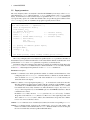
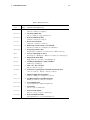
The data step below creates the datasetberkeley, a 2 × 2 × 6 table, classifying 4526 applicants to
graduate school at U.C. Berkeley in 1971 by Admission, Gender and Department.
berkeley.sas
title ’Berkeley Admissions data’;
data berkeley;
do dept = 1 to 6;
do gender = ’M’, ’F’;
do admit = 1, 0;
input freq @@;
output;
end; end; end;
/* Admit Rej Admit Rej */
cards;
512 313
89
19
353 207
17
8
120 205
202 391
138 279
131 244
53 138
94 299
5 EXAMPLES
22
16
17
1
2
3
4
5
6
7
8
24
351
24
317
;
The program lines below read this dataset, and use formats to recode the category levels into more
meaningful labels in a mosaic.
mosmat9.sas
%include catdata(berkeley);
proc format;
value admit 1="Admit" 0="Reject" ;
value dept 1="A" 2="B" 3="C" 4="D" 5="E" 6="F";
value $sex ’M’=’Male’
’F’=’Female’;
%table(data=berkeley, var=Admit Gender Dept, weight=freq, char=Y,
format=admit admit. gender $sex. dept dept.,
order=data, out=berkeley);
9
Admit
Admit
Admit
Reject
Reject
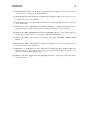
%mosmat(data=berkeley, vorder=Admit Gender Dept, sort=no, htext=3.5);
Female
A
B
C
D
E
F
A
B
C
D
E
F
Male
Gender
Reject
Dept
B
B
C
C D E F
D EF
Admit
Male
Female
Female
Male
A
A
10
Admit
Reject
Male
Female
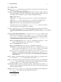
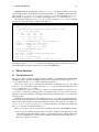
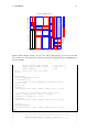
Figure 4: Mosaic matrix for Berkeley admissions data
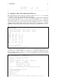
The TABLE macro is used (lines 4–6) translate the original variables into new variables which
have the formatted equivalents as their values (because SAS/IML still cannot read formatted values).
It was desired to retain the values of Sex in the order ‘Male’, ‘Female’, so ORDER=DATA was specified. (The sorted values, (Female, Male) produces a display where the labels are more crowded,
because there are fewer females). The new factors in the data set are all character variables.
The MOSMAT macro (line 10) produces Figure 4. SORT=NO keeps the program from messing
things up by sorting the data.
5.5 Example 5: Using PROC GENMOD and the MOSAIC macro
It was mentioned earlier that MOSAICS and the MOSAIC macro can be used to display the results
of models fit using PROC GENMOD or PROC CATMOD. Indeed, this is often the easiest way to use
MOSAICS and to visualize the results of a fitted model. It also allows you to fit more complex
models than can be handled by the IPF algorithm used internally in MOSAICS.
6 IMPLEMENTATION
1
25
We illustrate the process using the marital dataset shown in Section 5.2, fitting the model
[GPE] [PM] [EM] with PROC GENMOD.
mosaic5g.sas
%include catdata(marital);
2
3
4
5
6
7
proc genmod data=marital;
class Gender Pre Extra Marital;
model count = Gender|Pre|Extra Pre|Marital
/ dist=poisson obstats residuals;
ods output obstats=obstats;
Extra|Marital
8
9
10
%mosaic(data=obstats, var=Gender Pre Extra Marital,
vorder=Marital Extra Pre Gender, resid=streschi);
The essential idea is to fit this as a Poisson regression model for the count variable (lines 5–6), and
obtain a dataset containing residuals using the ODS OUTPUT statement (line 7).
The obstats dataset contains the original variables plus various residuals calculated by PROC
GENMOD, one of which is the standardized (adjusted) Pearson residual (called streschi). Feeding the obstats dataset to the mosaic macro (line 9) and specifying resid=streschi in the
macro call causes the program to bypass its built-in IPF fitting process, using the mosaicd module
described in Section 3.6.
5.6 Sample data sets
A variety of contingency tables are supplied with the MOSAICS distribution in the file mosdata.sas.
These are listed in Table 2, with the variable names and dimensions given in their order as in vnames.
Each data set is stored as a SAS/IML module containing definitions for the variables title,
dim, vnames, lnames, and table used in the run mosaics statement. Note that the variable
dim corresponds to levels in the arguments to mosaic. See the module haireye in Example
1.
The program mosdata.sas is set up so that running it will create a SAS/IML storage catalog
MOSDATA in the MOSAIC library. Once this has been done, any dataset may be obtained by loading
the module from MOSAIC.MOSDATA and running it. For example, the previous example could be
done using the module marital, as shown below.
1
2
3
4
proc iml;
reset storage=mosaic.mosdata;
load module=marital;
run marital;
5
reset storage=mosaic.mosaic;
load module=_all_;
6
7
8
9
10
11
12
13
14
ord = { 4,3,2,1};
run reorder(dim, table, vnames, lnames, ord);
split = {V H};
plots = 2:4;
run mosaic(dim, table, vnames, lnames, plots, title);
quit;
6
Implementation
This section describes the algorithm for the construction of mosaic displays and provides some notes
on the structure of the program.
6 IMPLEMENTATION
26
Table 2: Mosaics data sets
Module
name
bartlett
Ways
3
abortion
3
Title
Variable names(dimensions)
Bartlett data
Alive? (2) × Time (2) × Length (2)
Abortion opinion data
Sex (2) × Status (2) × Support Abortion (2)
berkeley
3
Berkeley Admissions Data
Admit (2) × Gender (2) × Dept (6)
cancer
3
Breast Cancer Patients
cesarean
4
Risk factors for infection in cesarean births
Survival (2) × Grade (2) × Center (2)
Infection (3) × Risk? (2) × Antibiotics (2) × Planned (2)
detergen
4
Detergent preference data
Temperature (2) × M-User? (2) × Preference (2) × Water softness (3)
dyke
5
Sources of knowledge of cancer
Knowledge (2) × Reading (2) × Radio (2) × Lectures (2) × Newspaper (2)
employ
3
Employment Status Data
gilby
2
Clothing and intelligence rating of children
EmployStatus (2) × Layoff (2) × LengthEmploy (6)
Dullness (6) × Clothing (4)
haireye
3
Hair color - Eye color data
Hair (4) × Eye (4) × Sex (2)
heckman
5
Labour force participation of married women 1967-1971
hoyt
4
Minnesota High School Graduates
1971 (2) × 1970 (2) × 1969 (2) × 1968 (2) × 1967 (2)
Status (4) × Rank (3) × Occupation (7) × Sex (2)
marital
4
Pre/Extramarital Sex and Marital Status
Marital (2) × Extra (2) × Pre (2) × Gender (2)
mobility
2
Social Mobility data
suicide
3
Suicide data
Son’s Occupation (5) × Father’s Occupation (5)
Sex (2) × Age (5) × Method (6)
titanic
4
Survival on the Titanic
Class (4) × Sex (2) × Age (2) × Survived (2)
victims
2
Repeat Victimization Data
First Victimization (8) × Second Victimization (8)
6 IMPLEMENTATION
27
6.1 Algorithm
The process is a naturally recursive one which can be implemented easily in a language which supports recursion and multi-dimensional arrays, such as APL or S/R. Wang [10] describes a FORTRAN
implementation of mosaic displays which simulates multi-dimensional arrays by subscripting a vector. The following algorithm, which uses two-dimensional arrays, is much simpler. A general scheme
for handling multi-dimensional arrays in SAS/IML is described in [6].
1. Denote the number of levels of the n variables by l1 , . . . , ln , and let Ls be their cumulative
products, Πsi=1 li . At step s = 0, start with one tile, a square of size 100 × 100, and let L 0 = 1.
2. The tiles in the mosaic are represented by an array B of four columns (called boxes in the
program). Columns 1 and 2 give the (x, y) location of the lower left corner of the tile; columns
3 and 4 give the horizontal and vertical lengths of the tile. At step 0, B = { 0 0 100 100 }.
There is one row for each tile. The following steps are repeated for each variable, s = 1, . . . , n:
3. For variable s find the marginal frequencies of variables s = 1, . . . , n, a vector of length L s ,
with the levels of variable s varying most rapidly.
4. Reshape this vector row-wise to a matrix M = {mgh } of Ls−1 rows and ls columns. (The
array M is called margin in the program. See the arrays labeled “Marginal totals” the printed
output.) The rows of M correspond to the tiles of the previous variables at step s − 1.
5. Each old tile is then divided vertically (if s is odd) or horizontally (s even) into l s tiles, with
the width (s odd) or height (s even) of each tile proportional to mgh /mg+ .
This computational scheme has several desirable properties:
• At any stage the division of the tiles for the current variable is in proportion to the entries in
each row of M divided by the row totals.
• We can draw the tiles representing the marginal frequencies at any stage, not just the final stage
as Hartigan and Kleiner [9] do.
• Fitting the model of joint independence of the current variable with all previous variables
jointly is equivalent to testing independence of the rows and columns of the matrix M. For
example, for a three-way table, the expected frequencies under the model [AB][C] can be expressed in terms of the IJ × K matrix M as m(ij)+ m+k /m++ .
6.1.1
Spacing
This procedure gives a mosaic of Ln = l1 × l2 × · · · × ln tiles with no spacing, in which cells with
small frequencies are difficult to see. Following Hartigan and Kleiner [9] the tiles are separated, with
larger spacings at the earlier subdivisions, to help preserve the visual impact of small counts. For a
four-way table with vertical splitting on variables 1 and 3, the divisions of the first variable are spaced
proportionally to 1/(l1 − 1); divisions between levels of the third variable are spaced proportionally
to 1/(l1 l3 − 1).
This spacing of the tiles is accomplished by constructing an unspaced mosaic in a reduced area
(determined by the space parameter), then expanding to include the necessary spacing. The boxes
array is initialized as
length= {100 100};
boxes = {0 0}
||( length - space );
/* x,y length of box area */
/* lowerleft x,y */
/* length
x,y */
Then, the (x, y) coordinates are multiplied by a diagonal matrix of scale factors sf, calculated from
the maximum (x, y) values of the upper-right corners, ur, of the tiles.
ur = boxes[,{1 3}][,+] || boxes[,{2 4}][,+];
max = max(ur[,1]) || max(ur[,2]);
sf = {100 100} / max;
6 IMPLEMENTATION
28
6.2 Program structure
mosaics.sas consists of 22 SAS/IML modules (subroutines and functions). The calling structure
of the modules is shown in Figure 5.
mosaic
*-- check inputs, assign default values;
|
|-- divide
*-- fit models and draw the mosaic display;
|
|--reduce
*-- find reduced model for factors 1:f;
|
|--mfit
*-- fits a specified model;
|
|--chisq
*-- calculate chisquares;
|
|--df
*-- calculate degrees of freedom;
|
|--terms
*-- find all terms in a loglinear model;
|
|--vars_in
*-- find variables in a term;
|
|--modname *-- expand config into string for model label;
|
|--divide1 *-- divide the mosaic for the next variable;
|
|--space
*-- space the tiles in the current display;
|
|--labels
*-- calculate label placements;
|
|--gboxes
*-- draw the current display;
|--fillbox
*-- custom shading;
|--glegend
*-- draw legend;
readtab
*-- read input frequencies, level names;
|--readlab
*-- read level names, reorder input
transpos
*-- reorder the dimensions of an n-way table;
Figure 5: Calling structure of the modules in MOSAICS
The top-level module, mosaic simply validates the input parameters, assigns default values for
global variables, and calls the module divide. The steps in the algorithm described above are
carried out by divide; the calculation of the new tiles in step 5 is performed in divide1.
The other top-level modules, readtab and transpos are included for convenience, to input a
frequency table into SAS/IML from a SAS dataset, and reorder table dimensions, respectively.
6.3 Changes
Version 3.6
•
•
•
•
Added an outstat global variable to generate an output data set with residuals, fitted, etc.
Module ’reorder’ changed to ’transpos’
Added a GOUT global variable for graphics catalog entry
Added WINDOW global variable to control window size
Version 3.5
• Fixed conflict between the global variable DEVTYPE and the macro variable used for graphics
device control.
• Changed circle blanking used for CELLFILL to white/black text, depending on shading density.
REFERENCES
29
• Added control of threshold for CELLFILL. You can now say CELLFILL = DEV 1.0 and
all absolute residuals > 1.0 will have their values written inp
the tiles.
• Added calculation and display of adjusted residuals ( = d/ (1 − h))
• The default font now depends on device driver, making it easier to get PS/EPS output in Windoze.
• Added NAME global variable for graph names in the graphics catalog.
• Fixed a bug in the calculation of adjusted residuals
• Added CELLFILL=’FREQ’ to display cell frequency in the tiles.
• Added ABBREV global to abbreviate variable names in models and titles.
Version 3.4
• Added vlabels global variable to control the number of variables for which variable names
are used in the display, fuzz now sets line style solid.
• Global variables are now set in a separate module to make changing defaults easier.
• In transpos module, you can now specify the variable names in the new order, rather than
indices. The config configuration may also be specified using variable names.
• Added code for models of joint independence and conditional independence in which any variable may be specified as the jointly independent or conditioning one.
Version 3.3
• Added a GSKIP module, for EPS (or GIF) output to separately named graphics files. Requires
a global macro variable, &DEVTYP = EPS
Version 3.2
• Added zeros= global input matrix to handle structural zeros.
• Added ability to display chisquare value in the mosaic title for each plot, by using ’&G2’ or
’&X2’ in the title string.
• Changed default values to filltype={HLS HLS}, colors={BLUE RED} since this is
what I always use now, except for monochrome output.
Version 3.1
• Added readtab routine for easier input from a SAS dataset.
• Added devtype=’FT’ to calculate and display Freeman-Tukey residuals.
• Character values of global input variables no longer need be entered in upper case.
Version 3.0
• Added ability to fit a sequence of Markov models (fittype=’MARKOV’;) for lag sequential
data.
• Fit the equiprobability model for the display of the first variable.
Version 2.9
• Installation simplified by creating a separate file, mosaicm.sas, to install IML modules.
• Filltypes changed to allow separate coding for positive and negative residuals, and to provide
grayscale shading levels.
• Added ability (cellfill) to print a symbol in the cell symbolizing the value of the residual.
References
[1] Friendly, M. (1991). SAS System for Statistical Graphics. Cary, NC: SAS Institute, 1st edn.
ISBN 1-55544-441-5. 1
REFERENCES
30
[2] Friendly, M. (1992). Mosaic displays for loglinear models. In ASA, Proceedings of the Statistical Graphics Section, pp. 61–68. Alexandria, VA. 1
[3] Friendly, M. (1994). Mosaic displays for multi-way contingency tables. Journal of the American
Statistical Association, 89:190–200. 1, 17
[4] Friendly, M. (1995). Conceptual and visual models for categorical data. The American Statistician, 49:153–160. 1
[5] Friendly, M. (1999). Extending mosaic displays: Marginal, conditional, and partial views of
categorical data. Journal of Computational and Graphical Statistics, 8(3):373–395. 1
[6] Friendly, M. (2000). Multidimensional arrays in SAS/IML. In Proceedings of the SAS User’s
Group International Conference, vol. 25, pp. 1420–1427. SAS Institute. 27
[7] Friendly, M. (2000). Visualizing Categorical Data. Cary, NC: SAS Institute. ISBN 1-58025660-0. 1
[8] Friendly, M. (2002). A brief history of the mosaic display. Journal of Computational and
Graphical Statistics, 11(1):89–107. 1
[9] Hartigan, J. A. and Kleiner, B. (1981). Mosaics for contingency tables. In W. F. Eddy (ed.),
Computer Science and Statistics: Proceedings of the 13th Symposium on the Interface, pp.
268–273. New York, NY: Springer-Verlag. 1, 27
[10] Wang, C. M. (1985). Applications and computing of mosaics. Computational Statistics & Data
Analysis, 3:89–97. 27