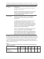
1
Microdata User Guide
Information and Communications
Technologies in Schools Survey
– 2003/04 –
April 2005
1
Information and Communications Technologies in Schools Survey, 2003/04 – User Guide
Table of Contents
1.0 Administration .............................................................................................................. 3
2.0 Authority ....................................................................................................................... 3
3.0 Background ................................................................................................................... 3
4.0 Objectives ..................................................................................................................... 4
5.0 Content.......................................................................................................................... 4
6.0 Uses............................................................................................................................... 5
7.0 Data Collection ............................................................................................................. 5
8.0 Data Processing............................................................................................................. 6
8.1 Data Capture ............................................................................................................. 7
8.2 Data Editing and Outlier Detection........................................................................... 7
8.3 Coding of “Other – Specify” Answers...................................................................... 8
8.4 Creation of Derived Variables .................................................................................. 8
9.0 Survey Methodology..................................................................................................... 9
9.1 Target Population.................................................................................................... 10
9.1.1 The Frame........................................................................................................ 10
9.1.2 First Nations schools ....................................................................................... 11
9.2 Sample Design ........................................................................................................ 11
9.3 Composition of Target Population.......................................................................... 11
10.0 Non-response ............................................................................................................ 12
11.0 Treatment of Non-response....................................................................................... 13
11.1 Adjustment Classes and Initial Adjustment Weights............................................ 14
11.2 Calibration............................................................................................................. 16
12.0 Quality Evaluation .................................................................................................... 16
12.1 Non-Sampling Errors ............................................................................................ 17
12.2 Coverage ............................................................................................................... 17
12.3 Non-response ........................................................................................................ 17
12.4 Data Capture ......................................................................................................... 22
12.5 Data Editing and Outlier Detection....................................................................... 22
13.0 Guidelines for Tabulation, Analysis and Release ..................................................... 23
13.1 Rounding Guidelines ............................................................................................ 23
13.2 Weighting Guidelines ........................................................................................... 24
13.3 Categorical vs. Quantitative Estimates ................................................................. 25
13.3.1 Categorical Estimates.................................................................................... 26
13.3.2 Quantitative Estimates ................................................................................... 26
13.4 Coefficient of Variation Release Guidelines ........................................................ 29
14.0 Variance Calculation................................................................................................. 32
14.1 Importance of the Variance................................................................................... 32
14.2 Excel-Based Coefficient of Variation Extraction Module.................................... 33
14.3 Using the Coefficient of Variation to Obtain Confidence Limits......................... 35
14.4 Hypothesis Tests ................................................................................................... 37
14.5 Coefficients of Variations for Quantitative Estimates .......................................... 37
Appendix A: Questionnaire .............................................................................................. 39
Appendix B: School Characteristics ................................................................................. 40
2
Information and Communications Technologies in Schools Survey, 2003/04 – User Guide
1.0 Administration
Sponsored by Industry Canada’s SchoolNet program, which works with Canadian
learning partners – provincial and territorial governments, education associations, school
boards, schools, teachers and students – and conducted by Statistics Canada, the
Information and Communications Technologies in Schools Survey (ICTSS) aims to
measure access to and integration of ICT into the learning environment. Support to the
initiative has been provided by the Library and Archives Canada.
Any questions about the data set or its use should be directed to:
Statistics Canada
Client Services
Centre for Education Statistics
Telephone: (613) 951-7608 or call toll free 1 800 307-3382
Fax: (613) 951-9040
E-mail: [email protected]
2.0 Authority
The Information and Communications Technologies in Schools Survey (ICTSS) was
conducted under the authority of the Statistics Act, Chapter S-19, Revised Statutes of
Canada 1985. Collection plans for the survey conformed with the requirement of
Treasury Board Circular 1986-19, Government Information Collection and Public
Opinion Research, and were registered under collection registration number STC/ECT165-75342.
3.0 Background
The ICTSS was sent to principals to collect reliable, baseline data on connectivity and
other aspects of ICT access in elementary and secondary schools across Canada. The
survey was developed be the Government of Canada’s SchoolNet program, in
cooperation with the SchoolNet National Advisory Board, and Statistics Canada.
In 2002, the Conference Board of Canada developed an analytical framework for
measuring school connectivity and ICT integration. Two elements of this analytical
framework – infrastructure and reach – were central to the ICTSS. Infrastructure includes
the different components of ICT that make up the underlying foundation of a connected
school, such as the number of computers and their characteristics. Reach refers to the
degree to which teachers and students have access to the ICT infrastructure.
3
Information and Communications Technologies in Schools Survey, 2003/04 – User Guide
4.0 Objectives
The data will be used to assess the current status of ICT infrastructure and reach and
some usage patterns in the schools, from a Canadian perspective. Survey findings will
also guide future policy and program development and provide the basis for future
research related to the use of ICT in learning. The survey data will also provide the
education authorities and the public with information in order to measure the quantity and
quality of the ICT infrastructure in Canadian schools and to develop programs and
policies aimed specifically at these schools.
5.0 Content
Participation in the survey was voluntary. Questionnaires were mailed out to all school
principals in October/November 2003, with the exclusion of First Nations schools for
which a separate mail out was administered in April/May 2004. Respondents were
offered the choice of answering to the survey using either the paper version or an on-line
application. A reproduction of this questionnaire is available in Appendix A.
The questionnaire was divided in thirteen sections:
1) Information about the school: Information about the number of full-time equivalent
teachers by sex, the number of students by sex and by grade, the number of
instructional rooms, the number of full-time equivalent employees devoted to the
school library, the annual expenses for the library’s collection, the sources of funding
for the library’s expenses and the location of the school.
2) Hardware: Information about the physical ICT infrastructure available in the schools
such as the number of computers available for educational purposes, the performance
levels of these computers as well as the student’s access to computers outside
instructional hours.
3) Software: Information about the types of software available in the school, and the
student’s access to this software.
4) Internet and Intranet Connections: Information about the Internet and intranet
connectivity in the school.
5) Internet and E-mail: Information about the use of Internet and e-mail in the school.
6) School website: Information about the school’s website, if one exists.
7) Videoconferencing: Information about the prevalence of videoconferencing in the
school.
4
Information and Communications Technologies in Schools Survey, 2003/04 – User Guide
8) Students’ online courses: Information about use of online courses for enrolled
students.
9) Teacher skills and professional development: Information about the skills and
professional development of teachers in the schools.
10) Technical support: Information about the technical support for the schools.
11) ICT Policy and Plans: Information about the policies and plans for ICT in the schools
or school boards.
12) Attitudes towards ICT: Information about the opinion of the principal about some
statements related to the ICT use in schools.
13) Challenges to ICT use: “Major” obstacles preventing the progression of ICT in the
school, according to the principal.
6.0 Uses
The microdata files have been made available to the school district/board (where
applicable), provincial/territorial ministry or department of Education, Industry Canada
and the Library and Archives Canada.
Industry Canada, through the SchoolNet program, will use the information in order to
assess the current status of ICT infrastructure and access and some usage patterns in the
schools, from a Canadian perspective. Survey findings will guide future policy and
program development and provide the basis for future research related to the use of ICT
in learning. The Library and Archives Canada is interested in using the data in order to
better understand the current infrastructure of all school libraries and to develop new
policies. Information provided to the school district/board and provincial/territorial
ministry or department of Education will allow them to measure the quantity and quality
of the ICT infrastructure in the school and to develop programs and policies aimed
specifically for the schools in the province/territory and district/board.
In addition to the publication of analytical studies related to the presence of ICT in
schools, this information will allow educational practitioners and policy makers to get a
better understanding of the areas where intervention and additional support measure are
needed.
7.0 Data Collection
Data collection took place from October 2003 to February 2004. Data were collected
directly from school principals who provided both the data available to them as well as
5
Information and Communications Technologies in Schools Survey, 2003/04 – User Guide
their views on ICT. In some cases, however, principals may have consulted or involved
others in gathering their responses.
A paper questionnaire and an Electronic Data Reporting (EDR) option were provided to
respondents for this survey. Each respondent was assigned a unique ID-number and ERD
password that was printed on the questionnaire along with name, address and telephone
number of the school. The respondents were asked to either complete the paper
questionnaire and mail it back using the envelope provided or complete the EDR
application.
Although participation in the survey was voluntary, a reminder fax was sent to
respondents, followed by telephone calls to encourage their participation. For cases in
which the timing of the interviewer's call was inconvenient, an appointment was arranged
to call back at a more convenient time.
If respondents were adamant about not having the time to complete the questionnaire then
they were offered the option of responding to a set of critical questions. For this option,
respondents were only asked to complete Questions 2, 3, 6, 15, 16 and 49 and to provide
consent to share the information about their school.
Question 2 – Number of full-time equivalent teachers by sex
Question 3 – Number of students by sex and grade
Question 6 – Number of instructional rooms by type
Question 15 – Number of desktop computers by type
Question 16 – Number laptops and notebooks by type
Question 49 – Perceived challenges in using ICT
Once a questionnaire was received, it was loaded into Blaise (collection system) and
predefined edits identified when data pertaining to the critical questions was missing. If
any such critical data was left out, an interviewer would then call the respondent to
inquire about the discrepancy and obtain the missing information. The interviewer also
had the option of coding each of these questions to either Refused or Don’t Know after
talking to the respondent. The edits related to Questions 2, 3, 6, 15, 16 and the question
regarding consent were considered hard edits, i.e. a follow-up with the respondent had to
take place to inquire about the discrepancy or to obtain the missing information. The
amount of follow-up that could be performed with the schools to correct values reported
by respondents was severely limited by the deadlines imposed after the collection period.
8.0 Data Processing
This chapter present a brief summary of the processing steps involved in producing the
microdata file.
6
Information and Communications Technologies in Schools Survey, 2003/04 – User Guide
8.1 Data Capture
Responses to survey questions were captured using one of two methods: Electronic Data
Reporting (EDR) and Intelligent Character Recognition (ICR). If the EDR option was
used then the respondent entered their data directly into the application and transmitted it
back to Statistics Canada via a secure ftp (File Transfer Protocol) site. If they completed
the paper questionnaire then the data was captured using ICR. The ICR technology
combines automated data entry (which uses optical character, mark and image
recognition) with supplementary manual capture by operators who ‘key from image’
some of the survey information using a heads-up data capture approach.
To ensure the quality of the captured data using ICR, all write-in fields were double
keyed for accuracy and a 20% quality control procedure was employed. For every batch
of captured questionnaires processed by the quality control operation, 20% of the
questionnaires were sampled and the images of these selected questionnaires were
compared to the actual data.
Range edits were programmed with the capture of both EDR and ICR. If information
entered was outside of the range (too large or small) of expected values, or produced an
inconsistency then the data would have been verified and changed or not accepted.
8.2 Data Editing and Outlier Detection
The data editing and outlier detection phases of processing involve the identification of
erroneous or inconsistent values in the survey data, and the modification of such
conditions.
The first type of error treated were errors in questionnaire flow. Conflicting
questionnaire information would sometimes indicate that a respondent had answered
questions in a section that in fact did not apply to them. In these cases, the superfluous
data was eliminated. An example of this type of error would be when a respondent
indicated in Questions 15 or 16 that they have computers connected to the internet but
then answers Question 23 which relates to the reason why the school has no internet
connection.
The second type of errors treated involved editing the survey records according to prespecified edit rules to check for logical inconsistencies in the survey data. In these cases a
strategy was established to eliminate the minimum amount of data, establishing priorities
so as to eliminate the values that were most likely to be in error. An example of this
would be when a respondent indicated that they had more teachers dedicated to the
library in Question 8 then the total number of teachers employed at the school in
Question 2. In this case, the responses to Question 2 were considered to be more likely to
be correct and therefore the offending cells from Question 8 were replaced by a code of
‘not stated’.
7
Information and Communications Technologies in Schools Survey, 2003/04 – User Guide
The third component of the editing process targeted the resolution of multiple answers to
the Likert-type scale questions (Questions 13, 21, and 47, for example). In responding to
these questions, some respondents marked multiple boxes (e.g. "Some" and "Many" in
Question 18). For each of these invalid records, one of the marked categories was chosen
at random. The adopted procedure respected the frequency with which categories where
reported among valid records (which marked only one box). For example, if an invalid
record marked "Some" and "Many" for an item in Question 18, which appeared 25 times
and 75 times respectively among the valid records, then the invalid record had a one out
of four chance of being assigned the value of "Some" and a three out of four chance of
being assigned the value "Many".
The fourth type of error dealt with assigning a code of ‘not stated’ whenever the
respondents did not provide any information to questions that should have been answered
Finally, the last type of error was related to the identification of outliers. Statistical
methods, based on either finding gaps in the distribution or values that were extremely
distant from the median, were used to examine distributions of numerical variables and
identify which values were extreme enough to warrant investigation. These methods
were applied not only to variables as captured in the survey, but also to ratios derived
from study variables (e.g. student-to-computer ratio, student-to-teacher ratio) and ratios
of study variables to frame variables (e.g. the ratio of the number of students gathered
from the survey to the number of students as presented on the frame). The most extreme
outliers were identified and the corresponding questionnaire images were checked to
ensure that the data was captured correctly. Those respondents whose extreme answers
seemed to be properly captured were contacted. In the end, approximately 50 records had
outlying values either confirmed or modified. This number of follow-ups was severely
limited by the deadlines imposed after the collection period.
8.3 Coding of “Other – Specify” Answers
A few data items on the questionnaire were recorded in an open-ended format such as the
“Other – Specify” questions. This type of write-in occurs when a question has a list of
possible response categories, as well as the option of stating another response not already
listed. In this situation the text was captured and then manually reviewed. If the write-in
was reflected in one of the existing categories, the response was recoded into the
appropriate category. Responses that could not be coded into an existing category where
left as a true “Other -Specify”.
8.4 Creation of Derived Variables
A number of variables on the microdata file have been derived by combining items on the
questionnaire or by using information on the frame in order to facilitate data analysis.
This may be done by using one variable or a combination of variables. The following is a
list of the derived variables for the ICTSS. Refer to Appendix B for a more detailed
8
Information and Communications Technologies in Schools Survey, 2003/04 – User Guide
description of derived variables related to school characteristics (Instructional level, size,
location of the school, as well as how the school is funded).
Variable
RuralDChosen
TotalMale_D
TotalFemale_D
Total_D
Typeschd
MINGRADE
MAXGRADE
GRADLVLD
Schsized
Numcompd_Q15
Numcompd_Q16
Numcompd
Intcond
Nintcond
Lowspdd
Medspdd
Highspdd
Otherspdd
Locclasd
Loclabd
Loclibd
Locothd
Stcomrd
Lowispdd
Medispdd
Highispdd
Otherispdd
Lociclad
Locilabd
Locilibd
Lociothd
Sticomrd
Desklcond
Laplcond
Totlan
Old_os
New_os
ProvCode
Description
School location (urban, rural)
Number of male students in all grades
Number of female students in all grades
Number of male and female students in all grades
Funding of school (public, private, mixed)
Minimum grade level of the school
Maximum grade level of the school
Instructional level of the school (elementary, secondary, mixed)
Size of the school (small, medium, large)
Number of desktop computers
Number of laptops and notebooks
Number of computers
Number of Internet-connected computers
Number of non-Internet-connected computers
Number of computers with low processor speed
Number of computers with medium processor speed
Number of computers with high processor speed
Number of computers with another processor speed
Number of computers in classrooms/portables
Number of computers in computer labs
Number of computers in libraries
Number of computers in other locations
Student to computer ratio
Number of Internet-connected computers with low processor speed
Number of Internet-connected computers with med. processor speed
Number of Internet-connected computers with high processor speed
Number of Internet-connected computers with another proc. speed
Number of Internet-connected computers in classrooms/portables
Number of Internet-connected computers in computer labs
Number of Internet-connected computers in libraries
Number of Internet-connected computers in other locations
Student to Internet-connected computer ratio
Number of desktop computers connected to the Internet
Number of laptops and notebooks connected to the Internet
Schools with an operating system for a local area network
Percentage of computers running on a less recent operating system
Percentage of computers running on most recent operating system
Province/Territorial code
9.0 Survey Methodology
9
Information and Communications Technologies in Schools Survey, 2003/04 – User Guide
This brief chapter describes the schools considered to be in-scope for this survey and the
final frame counts for each province and territory.
9.1 Target Population
The target population for the ICTSS is the set of all elementary and secondary schools in
Canada, excluding continuing education/adult day schools, trade/vocational schools,
language and cultural education schools, home schools, community education centres and
social service centres. The study includes schools in all provinces and territories as well
as schools located in aboriginal communities. Only schools open for the 2002/03 school
year were considered to be in scope for the ICTSS.
9.1.1 The Frame
The target population is accessed through the survey frame. The frame used for the
ICTSS is the 2002 Institution file: an administrative database of all Canadian elementary
and secondary schools maintained by the Centre for Education Statistics (CES) of
Statistics Canada. The Institution File contains a variety of information about each school
including contact information, the minimum and maximum grades of the school, how the
school is funded, and the number of students in the school.
CES gathers information from the most up to date sources reporting on elementary and
secondary schools in Canada every year in order to update the previous year’s Institution
File. Requests are then sent out to provincial ministries and/or school principals to update
each school’s information on the file. The Institution file that was used to create the
survey frame for the ICTSS contained all updates received through to the fall of 2003
following from requests sent in the fall of 2002.
Additional research activities were performed in the fall of 2003 in order to have the most
current information possible when conducting the survey. The focus of these activities
was on removing as many out-of-scope records and duplicate records as possible from the
list. For example, some records contained data suggesting that the school either had no
students or that adults were educated at the school despite having a valid school type.
These records were researched and some were eventually dropped from the frame as it
was confirmed that they were not in scope.
Some records on the frame were missing key analytical information. Research was
conducted to see if any of these missing values could be located, either online or in
Scott’s Directory of Canadian Schools. In conducting this research, it became apparent
that there were still some records on the frame that were out of scope. There were also
another four records that attached notes on the frame indicating that they were out of
scope – this information was confirmed and those schools were removed from the frame.
In order to identify duplicates that needed to be removed from the list, the frame was
sorted by a number of variables that, in combination, should have been unique identifiers
10
Information and Communications Technologies in Schools Survey, 2003/04 – User Guide
on the frame. These variables included a school’s name, address, postal code and phone
number.
After collecting and analysing the data, it was decided that virtual schools and distance
education schools (just like home schools) had very different characteristics than the
other types of schools contacted (in terms of student-to-computer ratio and usage of
computers on site, among other characteristics). As a result, they were also removed from
the scope of the survey.
9.1.2 First Nations schools
In preparation to distribute questionnaires to all elementary and secondary schools across
Canada, support was sought from various governing bodies. Contacts within the
provincial ministries of education were approached with regards to the majority of
Canada’s elementary and secondary schools. In order to contact First Nations schools in
Canada, however, special permission had to be granted by the various First Nations
Regional Management Organizations (RMOs). As this took more time than approaching
the provincial ministries, the set of First Nations schools on the frame had to be identified
and put aside from the initial mailing.
With the assistance of a list of First Nations schools in Canada provided to Statistics
Canada by the First Nations SchoolNet program at Industry Canada and the funding field
on the Institution File, over 400 schools were successfully identified as First Nations
schools and temporarily removed from the frame. Permission to contact First Nations
schools was eventually granted by the RMOs and the ICTSS questionnaires were sent out
in April of 2004.
9.2 Sample Design
As previously stated, all elementary and secondary schools in Canada that were
considered to be in scope as described earlier in this chapter were contacted to participate.
9.3 Composition of Target Population
Tables 1 and 2 outline the distribution of the schools contacted in October 2003 in the
main wave of the survey (excluding First Nations schools), by province and territory and
in terms of the five main analytical variables (instructional level, size, location, funding
and language of schools).
Table 1
Number of schools contacted for the ICTSS, by province and territory
Province/Territory
Population
Newfoundland
331
Prince Edward Island
72
Nova Scotia
475
11
Information and Communications Technologies in Schools Survey, 2003/04 – User Guide
New Brunswick
Quebec
Ontario
Manitoba
Saskatchewan
Alberta
British Columbia
Yukon
Northwest Territories
Nunavut
Total
366
3,013
5,634
820
808
1,880
2,020
29
52
41
15,541
Table 2
Number of schools contacted for the ICTSS, by the categories defined by key
analytical variables
Domain
Population
Elementary
10,121
Instructional Level
Secondary
3,404
Mixed
2,016
Small
4,970
Size
Medium
5,246
Large
5,325
Urban
11,455
Location
Rural
4,086
Public
13,704
Funding
Private
1,666
Mixed
171
English
12,225
Language
French
3,316
10.0 Non-response
Surveys’ response rates are measures of the effectiveness of the collection process and
are also good indicators of the quality of the estimates produced. Perhaps more so than
other surveys, the ICTSS is faced with multiple levels of non-response. This chapter will
provide a summary that distinguishes between three types of non-response: total, partial
and item non-response.
Total non-response:
For the sampled unit, the minimal set of critical questions was not collected. This
“minimal set of critical questions” refers to the set of critical questions defined in Chapter
7.0, with the exception of Question 2 (teacher counts) and Question 6 (instructional room
counts), which were determined to be less essential analytically than enrolment count or
12
Information and Communications Technologies in Schools Survey, 2003/04 – User Guide
consent to share information. Also, only one of Question 15 and Question 16 needed to
be answered, as it is completely acceptable for a school to have desktops but no portable
computers (or vice-versa). Weighting adjustment methods were used to compensate for
total non-response; this topic is discussed in more detail in Chapter 11.0 (refer to the first
phase weighting adjustments).
Partial non-response:
Only the minimal set of critical variables as defined for total non-response was collected.
Weighting adjustment methods were used to compensate for partial non-response. This
topic is discussed in more detail in Chapter 11.0.
Item non-response:
Item non-response could be associated with any questionnaire, except those in the total
non-response set. Item non-response refers to a limited absence of information for a small
number of variables, but all other variables (including the minimal set of critical
questions) within the questionnaire were collected. Item non-response is generally
corrected by techniques of imputation, although for the ICTSS the item non-response
rates were sufficiently low for most variables to avoid this process.
A total of 6,676 of the 15,541 schools covered in Table 1 provided usable information for
the survey (i.e. questionnaires were not identified in the total non-response set), for a
response rate of 43%. These formed a subset of the 7,311 returned questionnaires (a
return rate of 47%). A subset (6,103 questionnaires) of these usable questionnaires
answered more than just the critical questions and therefore did not display partial nonresponse (for a full response rate of 39%). More information on the occurrence of these
non-response issues can be found in Chapter 11.0 and Section 12.3.
11.0 Treatment of Non-response
Non-response is the major source of error for a survey such as the ICTSS. As this class of
errors is not generally random, it is important that it be minimized and also that a proper
adjustment strategy be derived to compensate for the presence of systematic non-response
patterns. Based on the analysis of the response rates, and operation constraints, the nonresponse patterns and the adjustment strategy were investigated using a two phase
approach:
Phase 1: Focussed on only the critical questions for all respondents (i.e. including
questionnaires with partial non-response).
Phase 2: Focussed on all questions for only those respondents that answered beyond the
critical questions (i.e. excluding questionnaires with partial non-response).
In each phase, the weight assigned to each school represents the number of other schools
in the population with similar characteristics. The weights were derived in two steps, as
described in Section 11.1.
13
Information and Communications Technologies in Schools Survey, 2003/04 – User Guide
These data sets were determined to have low item non-response rates for the majority of
both the critical questions (Phase 1) and the remaining questions (Phase 2).
Consequently, a weighting methodology based on key auxiliary information available on
the frame (i.e. province or territory, instructional level, size, location, funding and
language of school) was adopted to correct for total and partial non-response.
Unfortunately, some records on the frame were missing some key analytical information
needed to make this correction. For those cases, the missing data was imputed based on
information available from similar complete records. This resulted in imputing the
number of students and the instructional level for 3.1% and 0.3% of the frame’s records,
respectively.
11.1 Adjustment Classes and Initial Adjustment Weights
Explanatory analysis was applied, based on logistic regression, to investigate the
relationship between the key auxiliary information available (province or territory,
instructional level, size, location, funding and language of school) on the frame and the
probability of schools responding to the survey. As a result, schools were grouped into
several adjustment classes. These adjustment classes were constructed in such a way that
it could be assumed that within the class, each unit had the same probability of response.
The initial weight assigned to all schools belonging to an adjustment class was defined as
follows:
Phase 1 adjustment classes:
Number of schools in that class derived from the frame
W(Phase 1) = ------------------------------------------------------------------------Number of schools in that class that responded to the survey
Phase 2 adjustment classes:
Number of schools in that class that responded to the survey
W(Phase 2) = W(Phase 1) x -----------------------------------------------------------------------------------Number of schools in that class that responded beyond critical questions
Table 3 lists the first-phase non-response adjustment groups and the corresponding total
non-response rates. The rates are calculated as a proportion of the expected counts
derived from the ICTSS frame.
Table 3
Total Non-response by First-Phase Non-response Adjustment Class
Group
Frame
Group
Frame
Total NonTotal Nonresponse
response
Count Rate
Count Rate
Newfoundland
331
133 40.2% SK Med/Lrg.
66
28 42.4%
14
Information and Communications Technologies in Schools Survey, 2003/04 – User Guide
P.E.I.
Nova Scotia
New Brunswick
Quebec, English
Quebec, French
ON, English, Urban
ON, English, Rural
ON, French, Urban
ON, French, Rural
MB, Public or
Mixed
MB, Private
SK Large Elem.
SK Medium Elem.
SK Small Elem.
SK Large Mixed
SK Medium Mixed
SK Small Mixed
72
475
366
353
2,660
4,317
928
316
73
734
20
151
78
198
1,702
2,881
560
178
39
323
27.8%
31.8%
21.3%
56.1%
64.0%
66.7%
60.3%
56.3%
53.4%
44.0%
86
67
154
153
65
135
98
53
43
60
70
24
53
63
61.6%
64.2%
39.0%
45.8%
36.9%
39.3%
64.3%
Secondary
SK Small Secondary
AB Large Elem.
AB Medium Elem.
AB Small Elem.
AB Large Mixed
AB Medium Mixed
AB Small Mixed
AB Large Secondary
AB Med. Secondary
AB Small Secondary
BC Public
BC Private
BC Mixed Funding
Yukon
N-W Territories
Nunavut
70
233
304
254
239
176
205
93
188
188
27
81
138
126
125
88
136
38
91
112
38.6%
34.8%
45.4%
49.6%
52.3%
50.0%
66.3%
40.9%
48.4%
59.6%
1,682
260
78
29
52
41
1,022
151
35
5
15
18
60.8%
58.1%
44.9%
17.2%
28.8%
43.9%
The non-response adjustment groups created in the second-phase, together with the
corresponding partial non-response rates, are presented in Table 4. The rates are
calculated as a proportion of the set of all respondents.
Table 4
Partial Non-response by Second-Phase Non-response Adjustment Class
Partial NonGroup
Respondents
Group
Respondents
response
Count Conditional
Rate
Newfoundland
198
11
5.6%
ON,
412
Secondary
P.E.I.
52
4
7.7%
Manitoba
444
Nova Scotia
324
7
2.2%
Saskatchewan
440
New Brunswick
288
9
3.1%
Alberta
945
QC, Elementary
811
92
11.3%
BC Urban
648
QC, Mixed
60
2
3.3%
BC Rural
164
Level
QC, Secondary
242
11
4.5%
Yukon
24
ON Elementary
1,474
128
8.7%
N-W
37
Territories
ON, Mixed
90
2
2.2%
Nunavut
23
Level
15
Partial Non-re
Count
Co
25
53
45
75
89
12
0
2
6
Information and Communications Technologies in Schools Survey, 2003/04 – User Guide
Total and partial non-response varied primarily by province/territory (see Table 5 of
Section 12.3 for provincial and national non-response rates) and therefore the first classes
created each corresponded to a province or territory. Within some provinces/territories,
other factors were related to the response rate. For example, in Quebec, the logistic
regression analysis indicated that the likelihood that a school would respond depended on
whether it was a French school or an English school (as shown in Table 3). Therefore, the
Quebec class was divided into two classes: Quebec/English and Quebec/French. The
other sub-provincial classes were created in a similar fashion.
11.2 Calibration
Calibration estimation techniques are widely used in social surveys. They produce
estimates of totals for key variables that are consistent with known population counts.
This approach can also improve the quality of survey estimates if a relationship exists
between the key variables used in the calibration and the variables used for the
estimation.
To derive the final Phase 1 weights, initial weights defined in 11.1 were adjusted so that
estimated totals for key variables available on the frame equalled the corresponding
frame totals. For Phase 2, initial weights were adjusted so that estimated totals based on
schools that responded beyond critical questions (i.e. Phase 2 respondents) agreed with
corresponding estimates derived using final Phase 1 weights for all respondents (i.e.
Phase 1 respondents). For both phases, the initial weight adjustments were minimized
with respect to the squared difference between the final and initial weights (a technique
known as generalized regression estimation, or GREG).
Whenever possible, all categories of the key variables were used to adjust the weights
(for example with respect to funding types the estimated number of public, private, and
mixed funding schools would be ideally used to calibrate the weights). For some
provinces/territories however the small number of respondents available required that
some of those categories be collapsed (for example in Ontario the estimated number of
public or mixed schools was used to calibrate the weights).
12.0 Quality Evaluation
This chapter provides the user with information about the various factors affecting the
quality of the survey data. In a standard sample survey, there are two main types of
errors: sampling errors and non-sampling errors. A sampling error is the difference
between an estimate derived from a sample and the estimate that would have been
obtained from a census that used the same collection procedures. In the case of the
ICTSS, a census was taken and therefore no sampling error could have occurred. All
other types of errors are referred to as non-sampling errors and include frame coverage
problems, non-response, and processing errors, which are all discussed in the sections
16
Information and Communications Technologies in Schools Survey, 2003/04 – User Guide
below.
12.1 Non-Sampling Errors
There are many sources of non-sampling errors and these may occur at almost any phase
of a survey operation. Employees responsible for collection may misunderstand survey
instructions, respondents may misunderstand questions, or answers may have been
marked incorrectly on the questionnaire. Errors may also be introduced at any point when
the data is manipulated, including during the processing and tabulation of data.
For the ICTSS, quality assurance measures were established in order to reduce the
presence of non-sampling errors as much as possible. For example: initial contact with
provincial and territorial ministries or departments, school boards, relevant important
agencies relating to the target school population, and of course the school principals; the
questionnaires were tested; data collection follow-up activities were established including
the proper training of field staff; and edit quality checks were introduced to verify the
data coherency. For more information on Collection and Processing procedures, refer to
Chapters 7.0 and 8.0. Some of these measures provide indicators of the extent of nonsampling errors associated with the survey and are outlined below.
12.2 Coverage
The quality of the frame was assessed by examining under- and overcoverage, as well as
duplication of records. Difficulties arose in assessing the undercoverage of the frame as it
was determined that most of the other lists to which the Institution file could be compared
were either closely linked to the administrative files used to create the ICTSS frame,
related to previous version of these files, or lacking a common unique key. However, due
to the dynamic process of the annual school follow-ups and the annual comparison made
with aggregate figures released by provincial ministries, it is generally felt that the
undercoverage is quite low.
The processes explained in Section 9.1.1 that were used to detect duplicate records or
records that were out of scope yielded seven duplicated records and twenty-four out-ofscope records; these records were summarily removed from the frame. Considering the
scope of these processes, as well as the relatively small number of records requiring
removal, it is expected that the proportion of undetected duplicate and out-of-scope
records remaining on the frame is negligible.
To determine the quality of the imputed student counts on the frame (see Chapter 11.0)
the imputed data was compared to the enrolment data that Statistics Canada published for
the 1999/2000 school year. The results of this comparison suggest that the quality of the
imputation seems to be acceptable and the methodology involved sound. This and the
small proportion of such imputed cases (3.1%) both indicate that the imputation should
have a negligible impact on the survey estimates.
12.3 Non-response
17
Information and Communications Technologies in Schools Survey, 2003/04 – User Guide
If it can be safely assumed that total and partial non-response (defined in Chapter 10.0)
occurs completely at random, then it can be ignored. However, this is rarely the case;
typically the group of respondents and non-respondents exhibit different characteristics
and ignoring this can lead to the introduction of bias to survey estimates. As described in
Chapter 11.0, weighting adjustments were derived to minimize the risk of introducing
non-response-related bias to the ICTSS estimates.
Table 5 provides the distribution of non-response counts and rates by province and
territory for each phase, highlighting the 8,865 schools on the frame whose
questionnaires were not usable (total non-response), as well as the 573 respondents who
answered only the critical questions (partial non-response). The schools counted in the
“Frame” column are the same 15,541 in scope schools (excluding First Nations schools)
covered in Table 1. As described in Chapter 10.0, the total non-response schools are
schools that submitted a questionnaire that could not be considered usable as the minimal
set of critical questions was not provided. All rates are calculated as a proportion of the
expected counts derived from the ICTSS frame.
Table 5
Total and Partial Non-Response by province and territory
Total NonPartial
Total & Partial
Province Frame
response
Non-response
Non-response
and
territory
Count
Rate
Count
Rate
Count
Rate
NL
PE
NS
NB
QC
ON
MB
SK
AB
BC
YK
NT
NU
Canada
331
72
475
366
3,013
5,634
820
808
1,880
2,020
29
52
41
15,541
133
20
151
78
1,900
3,658
376
368
935
1,208
5
15
18
8,865
40.2%
27.8%
31.8%
21.3%
63.1%
64.9%
45.9%
45.5%
49.7%
59.8%
17.2%
29.8%
43.9%
57.0%
11
4
7
9
105
155
53
45
75
101
0
2
6
573
3.3%
5.6%
1.5%
2.5%
3.5%
2.8%
6.5%
5.6%
4.0%
5.0%
0.0%
3.8%
14.6%
3.7%
144
24
158
87
2,005
3,813
429
413
1,010
1,309
5
17
24
9,438
43.5%
33.3%
33.3%
23.8%
66.5%
67.7%
52.3%
51.1%
53.7%
64.8%
17.2%
32.7%
58.5%
60.7%
In order to assess the analytical utility of a particular question, it was also useful to look
at item non-response, or the degree to which each question was answered throughout the
survey for the set of respondents. Tables 6 and 7 indicate the non-response rates for most
questions after the data set was processed and inconsistent/outlying data were removed.
18
Information and Communications Technologies in Schools Survey, 2003/04 – User Guide
Furthermore, some questions served as “filters” in the sense that answers to these
questions determined the respondent’s flow through the questionnaire. For example, in
order to know whether a school should have provided an opinion of its technical support
in Question 43, it must first be known whether that school reported at least one hour of
technical support in Question 42 (which serves as the filter in this example). The nonresponse rates for these filter-dependent questions are presented in Tables 8 and 9.
Table 6
Non-response rates for the critical ICTSS questions
Question NonNonrespondents Response
Rate
2
94
1.4%
3
0
0.0%
6
33
0.5%
15
109
1.6%
16
315
4.7%
49
170
2.5%
Note: Critical Questions: 6,676 respondents
Table 7
Non-response rates for the non-critical ICTSS questions whose response rates did
not depend on answers to filter questions on the questionnaire
Question NonNonQuestion NonNonRespondents response
Respondents response
Rate
Rate
4
361
5.9%
32
430
7.0%
5
607
35
419
6.9%
9.9%
7
20
0.3%
37
226
3.7%
11
3,023 49.5%
38
362
5.9%
12
160
2.6%
39
202
3.3%
14
124
2.0%
40
4,008 65.7%
17
721 11.8%
41
628 10.3%
18
169
2.8%
42
579
9.5%
19
205
3.4%
44
242
4.0%
20
479
45
299
4.9%
7.8%
21
210
3.4%
46
384
6.3%
22
254
4.2%
47
250
4.1%
27
259
4.2%
48
258
4.2%
Notes:
Non-Critical, Filterless Questions: 6,103 Respondents
Highlighted are those questions with elevated non-response rates - the threshold was arbitrarily set at
7.5%
19
Information and Communications Technologies in Schools Survey, 2003/04 – User Guide
Clearly, due to their low response rates, results derived from Questions 11 and 40 will be
much less reliable than those derived from other questions. Results derived from the other
questions highlighted in Table 7 may also be unreliable.
For the remaining questions, the non-response rate is reported as a range instead of a
fixed value, as non-response to the appropriate filter question blurs the true degree of data
quality. It is known whether a respondent who answered a filter question should or should
not have answered the subsequent question(s). However, if a school did not provide data
of any sort to the filter question, then it is unknown as to whether they should have also
responded to the related follow-up question(s).
Diagram 1
Distribution of respondents passing through a filter question
All respondents
(A)
Responded to filter
(B)
Should not answer
follow-up to filter
(D)
Did not respond to filter
(C)
Should answer
follow-up to filter
(E)
Answered followup to filter
(F)
Did not answer
follow-up to filter
(G)
The problem in determining the non-response rate for the follow-up to a filter question is
that it is unknown how the respondents in box (C) would have been distributed across
boxes (B), (E) and (G), had they answered the filter question.
In table 8, the “filter passed” , “filter blanks” and “follow-up non-respondents” columns
correspond to boxes (E), (C) and (G) in Diagram 1, respectively. From left to right, the
three non-response rates on the right-hand side of the table are the lower and upper bound
on the non-response rate, as well as the projected value of this rate. These rates all take
the form [(G)+(X)]/[(E)+(X)], where (E) and (G) refer to the amount of respondents in
the corresponding boxes in Diagram 1, while (X) refers to the amount of respondents in
box (C) who would have been expected to answer the follow-up question, had they
indicated the appropriate response to the filter question.
The lower bound on the non-response rate refers to the case where (X) is 0, while the
upper bound refers to the case where (X) is all of (C). The projected value of the nonresponse rate is calculated by first taking the proportion (E)/(B) of respondents who
answered the filter question that should have answered the follow-up question and then
assuming that this proportion of respondents in (C) would also have been screened in.
20
Information and Communications Technologies in Schools Survey, 2003/04 – User Guide
This assumes that non-response to the filter question occurs randomly with respect to the
true distribution for the filter question.
Table 8
Non-response rates for the non-critical ICTSS filter-dependent questions
Question
Filter
Filter Filter
Follow-up
Lower
Upper
Question Passed Blanks
NonBound Bound
(E)
(C)
Respondents on N-R on N-R
(G)
Rate
Rate
8
7
5,726
14
297
5.2%
5.4%
9
7
5,726
14
734 12.8%
13.0%
10
7
5,726
14
320
5.6%
5.8%
Internet
23
189
36
35 18.5%
31.6%
cells in
24
5,878
36
333
5.7%
6.2%
questions
25
5,878
36
325
5.5%
6.1%
15
&
16
26
5,878
36
203
3.5%
4.0%
28
27
4,486
203
715 15.9%
19.6%
29
27
4,486
203
128
2.9%
7.1%
30
27
4,486
203
122
2.7%
6.9%
31
27
4,486
203
208
4.6%
8.8%
33
32
441
430
103 23.4%
61.2%
34
32
441
430
153 34.7%
66.9%
36
35
950
349
64
6.7%
31.8%
43
42
4,679
579
37
0.8%
11.7%
Projected
NonResponse
Rate
5.4%
13.0%
5.8%
19.0%
6.2%
6.1%
4.0%
18.7%
6.1%
6.0%
7.8%
28.8%
39.3%
12.1%
10.2%
Notes:
Non-response to Non-Critical Questions Relying on a Filter Question
Highlighted are those questions with elevated non-response rates
The only question whose non-response rate was not presented in any of the previous
tables is Question 13. While the first half of the question is open to all respondents, the
last half of the question should only be answered by schools with laptops and notebooks
and therefore, cell c0585 (No laptops or notebooks at this school) could be regarded as a
filter for these last six cells (c0428-c0433). The non-response rates for the four parts of
Question 13 are presented in Table 9. All 6,103 of the phase two respondents were
eligible to answer the first two sections, while only 2,861 clearly indicated in Question 16
that they had laptops or notebooks and were therefore eligible to answer the second half
of Question 13. A further 84 respondents did not indicate whether or not they had laptops
or notebooks.
Table 9
21
Information and Communications Technologies in Schools Survey, 2003/04 – User Guide
Non-response rates for Question 13 by type of computer.
Type of computer
Filter
Filter
Follow-up
Passed
Blanks
NonRespondents
Internet-connected
computers
Non-Internet-connected
computers
Internet-connected
laptops and notebooks
Non-Internet-connected
laptops and notebooks
6,103
----
Lower
Bound
on N-R
Rate
137
2.2%
6,103
----
300
4.9%
----
----
2,984
84
1,089
36.5%
38.2%
37.4%
2,984
84
1,132
37.9%
39.6%
38.8%
Upper
Bound
on N-R
Rate
----
Projected
NonResponse
Rate
----
Note:
Non-Response to Question 13 - only the second half of the question depended on a filter question
12.4 Data Capture
The ICTSS data capture operation was described in Chapter 8.0. As indicated, a quality
control operation was also conducted in which the entered data was compared to the entry
on the questionnaire itself to ascertain the effectiveness of the data capture process. The
quality control process enabled a systematic error in the data capture process to be
identified and corrected prior to the analysis of data.
12.5 Data Editing and Outlier Detection
The data editing and outlier detection processes were briefly described in Chapter 8.0.
Overall, 2,951 records triggered at least one of the 32 edits. The edits that were triggered
by the largest number of respondents were the following (note that the percentages below
refer to percentages of all phase 2 respondents):
•
14.0% (857) indicated in Question 13 that there were laptops or notebooks in the
school, but did not provide counts in Question 16.
•
6.8% (418) reported percentages of computers running on different operating
systems that did not add up to 100% (Question 20).
•
6.7% (408) reported no person-hours of technical support per month in Question
42, but then provided their opinions about the technical support they received in
Question 43.
•
5.8% (355) supplied a number of e-mail accounts provided to students (Question
25 – c0801) greater than the school enrolment count (Question 3).
22
Information and Communications Technologies in Schools Survey, 2003/04 – User Guide
No other phase 2 edit was triggered by more than 4.2% of the phase 2 respondents. As for
the phase 1 edits, none of them were triggered by more than 2.3% (156) of all
respondents.
As stated in Section 8.2, the number of follow-ups that could be performed with the
schools to correct reported outlying values was severely limited by the deadlines imposed
after the collection period. Due to these limitations, additional work to clarify outlying
relationships between certain numeric variables could not be performed. Ideally, more
schools would have been contacted to confirm or correct outlying values, particularly
those in Question 2 (in which many large teacher counts were reported) and in Question 4
(in which many high part-time student counts were reported).
13.0 Guidelines for Tabulation, Analysis and Release
This chapter provides an overview of the guidelines to be observed by users tabulating,
analysing, publishing or otherwise releasing any data derived from the ICTSS microdata
file. In particular, users of microdata following these guidelines should be able to
produce the same figures as those produced by Statistics Canada.
13.1 Rounding Guidelines
In order that estimates for publication or other release derived from the Information and
Communication Technologies in Schools Survey (ICTSS) microdata files correspond to
those produced by Statistics Canada, users are urged to adhere to the following guidelines
regarding the rounding of such estimates.
Estimates in the main body of a statistical table are to be rounded to the nearest hundred
units using the normal rounding technique. In normal rounding, if the first digit to be
dropped is from 0 to 4, the last digit to be kept is not changed. If the first or only digit to
be dropped is from 5 to 9, the last digit to be retained is increased by one. For example, in
normal rounding to the nearest hundred, if the last two digits are between 00 and 49, they
are changed to 00 and the preceding digit (the hundreds digit) is left unchanged. If the last
digits are between 50 and 99 they are changed to 00 and the preceding digit is
incremented by 1.
Marginal sub-totals and totals in statistical tables are to be derived from their
corresponding unrounded components and are then to be rounded themselves to the
nearest 100 units using normal rounding.
Averages, proportions, rates and percentages are to be computed from unrounded
components (i.e. numerators and/or denominators) and then are themselves to be rounded
to one decimal using normal rounding. In normal rounding to a single digit, if the final or
only digit to be dropped is 0 to 4, the last digit to be retained is not changed. If the first or
23
Information and Communications Technologies in Schools Survey, 2003/04 – User Guide
only digit to be dropped is 5 to 9, the last digit to be retained is increased by 1.
Sums and differences of aggregates (or ratios) are to be derived from their corresponding
unrounded components and then are to be rounded themselves to the nearest 100 units (or
the nearest one decimal) using normal rounding.
In instances where, due to technical or other limitations, a rounding technique other than
normal rounding is used, resulting in estimates to be published or otherwise released that
differ from corresponding estimates published by Statistics Canada, users are urged to
note the reason for such differences in the publication or release document(s).
Under no circumstances are unrounded estimates to be published or otherwise released by
users.
13.2 Weighting Guidelines
Although the ICTSS is a census of elementary and secondary schools across Canada, and
therefore has a very basic sample design, the survey non-respondents were not distributed
evenly across the population. As described in Chapter 10.0, a complex weighting scheme
was adopted to properly account for this behaviour. Using data from such complex
surveys presents problems for analysts as the procedures needed to offset non-response
affect the both the calculations of point estimates and variance estimates (see Section 14).
In order for point estimates to be as free from bias as possible for the ICTSS, survey
weights must be used.
When producing point estimates, including the production of ordinary statistical tables,
users must apply the appropriate weight. When producing estimates involving the critical
questions (i.e. Questions 2, 3, 6, 15, 16 and 49), the first phase weight scwght_p must be
used; every respondent provided data for these questions and therefore all responding
schools have a nonzero first phase weight. However, when generating estimates involving
non-critical questions, the second phase weight scwghtnp must be used; the set of
respondents who declined to answer the non-critical questions have a second phase
weight of 0. If the appropriate weights are not used, the estimates derived from the
microdata will not correspond to those produced by Statistics Canada. In addition,
producing estimates based on non-critical questions using phase one weights would yield
biased estimates, as these weights did not take partial non-response into consideration.
The weight assigned to each school can be viewed as the number of schools on the frame
represented by that particular respondent.
For some analysis techniques (for example linear regression, logistic regression, analysis
of variance or any other analysis where a measure of significance is required), it is
recommended that an adjusted weight be used. The method used to adjust weights rescales them so that the average weight is 1 and the sum of all weights is equal to the
sample size.
24
Information and Communications Technologies in Schools Survey, 2003/04 – User Guide
For example, suppose that analysis of all secondary schools is required. The steps to rescale the weights are as follows:
•
Select all respondents from the file who have been classified as secondary schools
(variable GRADLVLD=2).
•
Calculate the average weight for these records by summing the final school
weights (variable scwght_p or scwghtnp, depending on the variable of analysis)
from the microdata file for these records and then dividing by the number of
respondents who were classified as secondary schools.
•
For each of these respondents, calculate a rescaled weight equal to the final school
weight, divided by the average weight
•
Perform the analysis for these respondents using the rescaled weight.
This method of re-scaling weights can be useful for interpreting results provided by
standard statistical software. While many analysis procedures found in statistical
packages allow weights to be used, the meaning or definition of the weight in these
procedures differs from that which is appropriate in the framework of a survey such as
the ICTSS. The result is that while in many cases the point estimates produced by the
packages are correct, the variance estimates that are calculated are poor. Furthermore,
these estimates might not match those available from Statistics Canada due to the way
certain software packages treat the weight field. Re-scaling weights can make the
variances calculated by standard software packages more meaningful by incorporating
the unequal probabilities of selection. One benefit of adjusting the weights is that an
overestimation of a level of significance, which is very sensitive to sample size, is
avoided while maintaining the same distributions as those obtained when using the final
weight.
When using standard statistical software to calculate estimates based on re-scaled
weights, the variability of the estimates inherent in the non-response mechanism is still
not taken into account. Therefore the variance estimates calculated in this way likely
underestimate the true variance. The calculation of more precise variance estimates
requires detailed knowledge of the assumed non-response behaviour of the survey
population and the corresponding adjustment procedure adopted. For more information
on calculating variance estimates for the ICTSS, refer to Chapter 14.0.
13.3 Categorical vs. Quantitative Estimates:
The unit of analysis in the ICTSS file is the school. Although other estimates can be
derived from the ICTSS, the weights attached to each record (scwght_p and scwghtnp)
were designed to provide reliable estimates of proportions based on school counts. For
example, the estimate of the proportion of students enrolled in schools reporting a
website may not be as reliable as the estimate of the proportion of schools indicating that
they have a website.
25
Information and Communications Technologies in Schools Survey, 2003/04 – User Guide
Before discussing how the ICTSS data can be tabulated and analysed, it is useful to
describe the two main types of point estimates of population characteristics that can be
generated from the ICTSS microdata file. To simplify the discussion, it is assumed in the
following descriptions that the proper set of respondents is used. This depends on
whether only critical variables are needed (Phase 1 respondents) or some non-critical
variable is needed (Phase 2 respondents). In addition, the reference to a domain in the
following discussion refers to a group of schools for which an estimate is to be generated
(for example, one such domain would be the set of schools located in a particular
province or territory).
13.3.1 Categorical Estimates
Categorical estimates are estimates of the number or percentage of the surveyed
population possessing certain characteristics or falling into some defined category.
Whether a school has videoconferencing capabilities or has an ICT policy in place are
examples of such estimates.
Examples of Categorical Questions:
Q:
What type of website does your school have on the Internet?
R:
Formal site / Informal site / No website
Q:
Does your school have a written acceptable use policy for student use of
technology?
R:
Yes / No
13.3.2 Quantitative Estimates
Quantitative estimates include estimates of totals or of means, medians and other
measures of central tendency of quantities based upon some or all of the members of the
surveyed population. They also specifically involve estimates of the form Xˆ / Yˆ , where
Xˆ is an estimate of the surveyed population quantity total and Yˆ is an estimate of the
number of schools in the surveyed population contributing to that total quantity, or other
more complex estimates such as regression coefficients.
An example of a quantitative estimate is the average annual expenditures by a school for
development of its library collection. The numerator is an estimate of the total amount of
money spent on developing a library’s collection, and the denominator is an estimate of
the total number of schools having a library.
Examples of Quantitative Questions:
Q:
How many computer labs do you have in your school?
R:
|_|_| labs
26
Information and Communications Technologies in Schools Survey, 2003/04 – User Guide
Q:
How many digital recording devices (used only for educational purposes) are
there at your school?
R:
|_|_|_|_| devices
13.3.3 Tabulation of Categorical Estimates
Number of schools possessing a certain characteristic
When all respondents in the domain answered the question related to the characteristic of
interest (i.e. no item non-response is observed), the estimate can be obtained from the
microdata file by summing the final weights of all records in the domain possessing this
characteristic.
If item non-response exists in the domain for the relevant question, the estimate can be
derived in two steps, as described below. This approach is appropriate only if the
observed item non-response is small (say less than the arbitrarily set threshold of 7.5%
used in Section 12.3).
Step 1: calculate the proportion of responding schools in the domain with this property
(see procedure below for proportions)
Step 2: multiply this proportion by the sum of weights for all schools in the domain.
Proportions of the form Xˆ Yˆ :
(a) Add up the final weights of records having the characteristic of interest for the
numerator ( Xˆ ),
(b) obtain Yˆ by adding together the final weights of records for all schools in the domain,
excluding those who did not respond to the question used to identify the characteristic,
(c) divide estimate a) by estimate b) ( Xˆ / Yˆ ).
13.3.4 Tabulation of Quantitative Estimates
Estimating population totals
Estimates of quantities can be obtained from the microdata file by multiplying the value
of the variable of interest by the final weight for each record, when every respondent
from that domain provided that information, then summing this quantity over all records
of interest. As with the case of categorical estimates, if item non-response exists in a
particular domain for the relevant question, then that estimate must be derived in two
steps, as described below.
Step 1: obtain the average value of the quantity of interest for responding schools in the
domain by using the procedure below for ratios.
27
Information and Communications Technologies in Schools Survey, 2003/04 – User Guide
Step 2: multiply this average by the sum of weights for all schools in the domain.
In the case that the quantitative variable is correlated to the school’s enrolment, one can
increase the precision of the estimate by using this auxiliary information. The following
approach only works for variables correlated to the student count, as there are no other
variables obtained in this study for which no item non-response was observed.
Step 1: obtain the average value of the quantity of interest per student in the domain by
using the procedure below for calculating ratios, but altering step b) to derive Yˆ by using
student counts as the variable of interest.
Step 2: take the sum of the products of each record’s weight and student count, for all
schools in the domain.
Step 3: multiply the average obtained in Step 1 by the sum from Step 2.
Also note that the approaches in this section are only appropriate if the item non-response
pertaining to the relevant question in the domain of interest is small (say less than the
arbitrarily set threshold of 7.5% used in Section 12.3).
Proportions and ratios of the form Xˆ Yˆ :
(a) Add up the products of the value of the variable of interest for the numerator and final
weight of records in the domain for the numerator ( Xˆ ), excluding those who did not
respond to the variables of interest corresponding to the numerator or the denominator.
(b) obtain Yˆ by adding together the products of the value of the variable of interest for
the denominator and the final weights of records for all schools in the domain, excluding
those who did not respond to the variables of interest corresponding to the numerator or
the denominator.
(c) divide estimate a) by estimate b) ( Xˆ / Yˆ ).
For example, to estimate the proportion of computers in urban schools that have a low
processor speed,
•
estimate the total number of computers in urban schools that have a low processor
speed ( Xˆ ) by summing up the product of the number of computers that have a
low processor speed and the final weights for urban schools (in this case all
schools are expected to have answered the questions on number of computers),
•
estimate the total number of computers in urban schools ( Yˆ ) by summing the
product of the number of computers and the final weights of all urban schools,
28
Information and Communications Technologies in Schools Survey, 2003/04 – User Guide
•
divide the first estimate by the second estimate ( Xˆ / Yˆ ).
13.4 Coefficient of Variation Release Guidelines
Before releasing and/or publishing any estimate from the ICTSS, users should first
determine the quality level of the estimate. The standard quality levels are: acceptable,
marginal and unacceptable. Data quality is typically affected by both sampling and nonsampling errors.
However, as discussed in Chapter 12.0, the quality of an estimate derived from the ICTSS
is based solely on the non-sampling errors. An important indicator of this quality is the
variability related to non-response and the corresponding adjustments reflected in the
coefficient of variation, as described in Chapter 14.0. The relationship between the
standard levels of quality and the coefficient of variation is illustrated in Table 10. Users
should also read Chapter 12.0 to be more fully aware of the quality characteristics of
these data.
In establishing the standard quality level of an estimate, the user should first determine
the number of respondents that contributed to the calculation of the estimate. If this
number is five or less, the weighted estimate should not be released in order to respect
policies regarding confidentiality. For weighted estimates based on sample sizes of
greater than five, users should determine the coefficient of variation of the estimate and
follow the guidelines below. These quality level guidelines should be applied to weighted
rounded estimates. Any estimate of marginal or unacceptable quality level must be
accompanied by a warning to caution subsequent users.
Table 10
Quality level guidelines based on the CV of a particular estimate
Quality Level of
Guidelines
Estimate
1) Acceptable
Estimates have:
A sample size of more than 5 and coefficients of variation in
the range of 0.0% to 16.5%.
No warning is required.
29
Information and Communications Technologies in Schools Survey, 2003/04 – User Guide
2) Marginal
Estimates have:
A sample size of more than 5 and coefficients of variation in
the range of 16.6% to 33.3%.
Estimates should be flagged with the letter M (or some similar
identifier). They should be accompanied by a warning to
caution subsequent users about the high level of error
associated with the estimates.
3) Unacceptable
Estimates with a sample size of five or less should not be
released, in order to respect Agency policies regarding
confidentiality.
For estimates with a sample size of more than five, but with
very high coefficients of variation in excess of 33.3%,
Statistics Canada recommends not releasing these estimates,
due to their unacceptable level of quality. However, if the user
chooses to do so, then these estimates should be flagged with
the letter U (or some similar identifier) and the following
warning should accompany the estimates:
“Please be warned that these estimates [flagged with the letter
U] do not meet Statistics Canada’s quality standards.
Conclusions based on these data will be unreliable and, most
likely, invalid. These data and any consequent findings should
not be published. If the user chooses to publish these data or
findings, then this disclaimer must be published with the data.”
To illustrate the concept of coefficients of variation, a table of CVs produced for a variety
of ICTSS estimates is presented below. Please note that the estimated CV of 0.00% listed
for the proportion of Yukon schools with Always-on connection to the internet comes as
a result of all participating schools indicating that they connected to the Internet in this
manner. This does not mean that all of the non-responding schools in the Yukon have an
Always-on connection as well.
Table 11
Estimates of the coefficient of variation for several key characteristics by province
and territory, 2003/04
Proportion of computers by Internetconnectivity
Internet-connected
Non Internet-connected
Canada
Newfoundland
and Labrador
Prince
Edward
Island
Nova
Scotia
New
Brunswick
Quebec
Ontario
0.18%
2.35%
0.62%
8.31%
1.38%
15.44%
0.36%
8.26%
0.24%
6.13%
0.52%
5.51%
0.32%
4.90%
30
Information and Communications Technologies in Schools Survey, 2003/04 – User Guide
Proportion of computers by
1
processor speed
Low speed
Medium speed
High speed
Other speed
1.25%
0.74%
2.12%
9.53%
3.59%
2.97%
7.60%
x
7.03%
5.08%
32.88%
x
5.05%
2.64%
8.27%
29.56%
1.91%
3.10%
3.12%
18.28%
2.26%
1.73%
5.80%
31.08%
2.71%
1.32%
3.99%
19.21%
Proportion of schools by methods to
access the Internet
2
Dial-up access
3
Always on connections
Student-to-computer ratio (median)
3.43%
0.46%
0.66%
9.63%
1.61%
3.18%
x
5.77%
4.77%
x
0.95%
1.87%
16.18%
0.66%
1.44%
7.02%
1.01%
1.85%
7.44%
0.95%
0.96%
Manitoba
Saskatchewan
Alberta
British
Columbia
Yukon
Northwest
Territories
Nunavut
Proportion of computers by Internetconnectivity
Internet-connected
Non Internet-connected
0.80%
6.26%
0.41%
6.79%
0.38%
4.97%
0.54%
5.20%
1.74%
x
0.70%
17.54%
2.18%
15.85%
Proportion of computers by
1
processor speed
Low speed
Medium speed
High speed
Other speed
4.20%
3.01%
6.25%
20.55%
4.93%
3.73%
6.30%
16.39%
3.07%
1.61%
3.43%
20.38%
3.02%
1.94%
6.07%
21.57%
4.83%
5.69%
17.04%
x
8.44%
6.99%
9.19%
x
13.60%
11.44%
20.82%
x
Proportion of schools by methods to
access the Internet
2
Dial-up access
3
Always on connections
Student-to-computer ratio (median)
8.03%
1.52%
2.60%
16.35%
1.26%
1.72%
8.21%
1.18%
1.32%
11.44%
1.19%
1.45%
x
0.00%
4.28%
x
6.43%
8.12%
x
22.86%
20.62%
Table 12
Estimates of the coefficient of variation for several key characteristics by type of
school, 2003/04
All schools
Instructional level of
school
Location of
school
Elementary
Secondary
Urban
Rural
0.18%
0.25%
0.30%
0.21%
0.34%
2.35%
2.55%
5.97%
2.80%
3.86%
Low speed
1.25%
1.36%
2.60%
1.47%
2.18%
Medium speed
0.74%
0.95%
1.26%
0.84%
1.47%
High speed
2.12%
2.56%
3.52%
2.45%
3.93%
Other speed
9.53%
10.00%
22.90%
10.78%
18.36%
Proportion of computers by Internet-connectivity
Internet-connected
Non Internet-connected
1
Proportion of computers by processor speed
Proportion of schools by methods to access the Internet
2
Dial-up access
3
Always on connections
3.43%
4.43%
11.59%
6.12%
4.08%
0.46%
0.61%
0.67%
0.48%
1.20%
0.66%
0.73%
1.17%
0.68%
1.34%
Student-to-computer ratio (median)
Canada
31
Information and Communications Technologies in Schools Survey, 2003/04 – User Guide
14.0 Variance Calculation
While the ICTSS is not a probabilistic survey, in the sense that no sample was selected to
represent the population, there is still an amount of variability in the estimates due to nonsampling errors. An important component of this variability is inherent in the patterns of
response and the adjustments made to take the non-responding elements into account.
This chapter explains why it is important to calculate the variance and presents different
tools to do so.
14.1 Importance of the Variance
The variance of an estimate is a good indicator of the estimate’s quality. An estimate
accompanied by a high variance is considered to be unreliable. In order to quantify the
degree of variance, a relative measure of the variability is used, namely the coefficient of
variation, or CV.
The coefficient of variation is defined as the ratio of the square root of the variance (also
known as the standard deviation, or standard error) to the estimate itself. The coefficient
of variation, as opposed to the variance, allows the analyst to compare estimates of
different magnitudes on a common scale. As a result, it is possible to assess the quality of
any estimate using the CV.
Determining the true variance, and hence the true CV, for an estimate is only possible if
the corresponding characteristic of interest is known for all schools in the target
population. The alternative, when feasible, is to estimate the variance based on the set of
respondents. To simplify the discussion throughout this document, references to the
variance and CV in this chapter will refer to their estimated values.
The Role of the Critical Questions in Variance Estimation
The method applied in approximating the variance of an estimate differs depending on
whether the estimation was based only on critical questions (i.e. Questions 2, 3, 6, 15, 16
and 49), or also on non-critical questions. When only critical questions were needed to
produce an estimate, the standard error estimate was derived in one phase based on all
respondents to the survey. However when non-critical questions were used, it was
necessary to proceed in two phases. The first phase involved all respondents, and the
second phase only the subset of respondents that answered more than just the critical
questions. For example, the standard error for the average number of Internet-connected
computers per school (Questions 15 and 16) was derived in one phase. However the
standard error for the percentage of schools with word processing software available to
students (Question 18) required a two-phase approach.
Method to Obtain the Variance of an Estimate
32
Information and Communications Technologies in Schools Survey, 2003/04 – User Guide
It is possible, under the assumptions made on the non-response mechanism described in
Chapter 10.0, to derive an exact formula to estimate the variance for every point estimate
in the ICTSS. However, performing this for each estimate that could be generated for the
ICTSS would be an extremely costly procedure and, for most users, an unnecessary one.
One user-friendly tool has been developed to help users calculate the variance and the
CVs for their estimates. This tool is an Excel-based CV extraction module (CVEM) that
produces approximate CVs for a large number of domains. The CVEM is designed
mainly for proportions, although it can provide rough approximates of CVs for others
simple statistics (for example totals for categorical variables).
It is also worth noting that all CVs in the CVEM are approximate and, therefore,
unofficial. Estimates of actual CVs for specific variables may be obtained from Statistics
Canada on a cost-recovery basis. The use of official estimates of CVs might allow users
to release otherwise unreleasable estimates, i.e. estimates with CVs in the “restricted”
range.
14.2 Excel-Based Coefficient of Variation Extraction Module
The Microsoft Excel-based CV extraction module (CVEM), developed with Excel
macros and accessed through a user-friendly interface, has been primarily designed to
allow users to extract CVs for proportion estimates derived from categorical variables in
the ICTSS. While the tool can also be used to extract CVs for estimates of totals for
categorical variables, it should be noted that these could be less reliable than proportion
CVs, except in the special case where the corresponding variable exhibit no item nonresponse. The CVs can be extracted in two ways, as described below.
The first way to extract a CV from this tool is by defining the domain of interest using the
following five analytical variables: the province/territory (ProvCode) in which a school is
located, whether a school is urban or rural (RuralDChosen), the way in which a school is
funded (TypeSchD), and the instructional level (GradLvlD) and size (SchSizeD) of a
school. The second method involves the specification of the size of the domain of
interest. The information displayed consists of the proportion estimate, the number of
respondents in the specified domain, the estimated population in that domain, basic
statistics (the variance, standard error and 95% confidence interval corresponding to the
population point estimate), and the coefficient of variation for the selected proportion.
Over 200 domains are covered by the CVEM. At the national level, users are able to
extract CVs from any domain made from the crossing of at most two of the analytical
variables (for example, by instructional level, or by size and funding, but not by funding,
instructional level and location). At the provincial/territorial level, CVs from any domain
formed by the inclusion of at most one of these variables (for example, by Manitoba or by
Quebec and funding, but not by Alberta and instructional level and size) can be extracted.
An approximate CV was generated for eight different proportions in each of the domains,
for a total of over 1,600 CVs. However, CVs corresponding to domains in which five or
fewer records contributed to the proportion in question have been suppressed.
33
Information and Communications Technologies in Schools Survey, 2003/04 – User Guide
Simulations based on 100 repetitions and assuming no item non-response, were run to
estimate variances, coefficients of variation and confidence intervals at the 95% level for
different proportions, i.e. 1%, 5%, 10%, 15%, 20%, 30%, 40% and 50%. In order to
estimate the CV for a proportion greater than 50%, one can obtain the CV for the
proportion of 50% and assume that the desired CV will be less than this quantity. One
can also use the fact that the standard error for a proportion p is equal to the standard
error for the corresponding proportion (1- p) to obtain a CV for a proportion exceeding
50%. For example, if the CVEM shows that the CV for a proportion p is 0.06, then the
CV for (1- p) is
CV=0.06*( p)/(1- p)
As mentioned in Chapter 13.0, users should always check the quality of the estimates,
especially for smaller proportions obtained from small domains. To help users identify
high CVs, colour coding has been used in the Excel application when displaying a CV.
CVs in excess of 50% have been coloured red, those in the range of 33.3% to 50% are
orange and those in the range of 16.6% to 33.3% are yellow. Refer to Section 13.5 for
more information regarding coefficient of variation release guidelines for the ICTSS. For
more information on quality guidelines for Statistics Canada products, refer to the
publication entitled: Statistics Canada Quality Guidelines, Catalogue no. 12-539-XIE.
In order to derive CVs for Categorical Estimates using the data in the CVEM, some rules
need to be applied.
Rule 1: Estimates of Number of Schools Possessing a Characteristic (Aggregates)
Given that the CVEM does not take item non-response into account, it is safe to say that
an estimate’s CV is close to (though slightly greater than) that of the proportion it
represents, provided the corresponding item non-response is small. Hence, to get an
approximation of an estimate’s CV, users could use the CVEM by specifying the
domain’s size and deriving the appropriate proportion. This procedure should only be
employed when the item non-response for the question relating to the characteristic is
small (say less than the arbitrarily set threshold of 7.5% used in Section 12.3) and the size
of the domain of interest is relatively large. In general, provincial/territorial estimates will
be reliable, but the reliability of sub-provincial/territorial estimates depends on whether
the domain is related to the non-response adjustments groups or to the set of totals used to
calibrate the weights.
For example, suppose we have an estimate Yˆ = 30,000 schools possessing a certain
characteristic. If we are to compare them to the 100,000 schools in the domain of interest,
then the CV for Yˆ should be close to the CV of the proportion (which, in our example, is
30,000 / 100,000 = 30.0%).
Rule 2: Estimates of Proportions or Percentages of Schools Possessing a
Characteristic
34
Information and Communications Technologies in Schools Survey, 2003/04 – User Guide
The CVs calculated in the CVEM are for proportions. Hence, they can be used directly as
they are given on the spreadsheet. However, they are only valid if item non-response is
small (say less than the arbitrarily set threshold of 7.5% used in Section 12.3). Therefore,
it is not recommended to use the CVEM to estimate the CV of proportions involving data
from Questions 11 or 40.
Rule 3: Estimates of Differences Between Aggregates, Percentages and Ratios
The standard error of a difference between two estimates is approximately equal to the
square root of the sum of squares of each standard error considered separately. That is,
the standard error of difference ( dˆ = Xˆ 1 − Xˆ 2 ) is approximated by:
σ dˆ = ( Xˆ 1α 1 ) 2 + ( Xˆ 2α 2 ) 2
where α 1 and α 2 are the CVs of Xˆ 1 and Xˆ 2 respectively. The CV of dˆ is given by
dividing its standard error by dˆ itself. This is a good approximation for the CV of a
difference between separate and uncorrelated characteristics, but may not be accurate
otherwise as it will tend to overstate the CV if Xˆ 1 and Xˆ 2 are positively correlated and
understate the CV if Xˆ and Xˆ are negatively correlated. Estimates of CVs for
1
2
correlated Xˆ 1 and Xˆ 2 may be obtained from Statistics Canada on a cost-recovery basis.
Rule 4: Estimates of Ratios
In the special case where the ratio represents a proportion or percentage of schools
possessing a characteristic then one can use the CVEM as in Rule 2. Otherwise, the
standard error of the ratio of the estimates is approximately equal to the square root of the
sum of squares of each CV considered separately, multiplied by the ratio itself. That is,
the CV of such a ratio Rˆ = Xˆ 1 / Xˆ 2 is
α Rˆ = α 1 2 + α 2 2
where α 1 and α 2 are the CVs of Xˆ 1 and Xˆ 2 respectively. As with the CV estimate of
Rule 3, this estimate will tend to overstate the CV if Xˆ and Xˆ are positively correlated
1
2
and understate the CV if Xˆ 1 and Xˆ 2 are negatively correlated.
Rule 5: Estimates of Differences of Ratios
This is simply a combination of Rules 3 and 4. The CVs for the two ratios are first
determined using Rule 4 and then the CV of their difference is found using Rule 3.
14.3 Using the Coefficient of Variation to Obtain Confidence Limits
35
Information and Communications Technologies in Schools Survey, 2003/04 – User Guide
Although coefficients of variation are widely used, a more intuitively meaningful
measure of sampling error is the confidence interval of an estimate. A confidence interval
constitutes a statement on the level of confidence that the true value for the population
lies within a specified range of values. In the case of the ICTSS, where a census rather
than a sample was used as the means of contacting potential respondents, the variability
in the estimates is primarily due to the observed non-response. As the non-response
adjustments made were contingent on the number of respondents in each adjustment
class, the interpretation of a 95% confidence interval is that if the census were carried out
an indefinite number of times and in each case the number of respondents in each
adjustment class was constant, then 95% of the response sets would generate estimates
whose confidence intervals would contain the true value.
Confidence intervals for an estimate, Xˆ , are generally expressed as two numbers, one
below and one above the estimate, as in ( Xˆ ± k ), where k is determined depending upon
the level of confidence desired and the standard error of the estimate. As the true standard
error of the estimates is unknown, confidence intervals are estimated based on the set of
respondents.
Using the standard error of an estimate, confidence intervals for estimates may be
obtained under the assumption that with a large enough sample size, the various estimates
obtained for a population characteristic are normally distributed about the true population
value. Under this assumption, the chances are about 68 in 100 that the difference between
a sample estimate and the true population value would be less than one standard error,
about 95 out of 100 that the difference would be less than two standard errors, and about
99 out of 100 that the differences would be less than three standard errors. These different
degrees of confidence are referred to as the confidence levels.
The 95% confidence intervals for an estimate are available directly in the CV
spreadsheet. If the user wants to determine other confidence intervals, the following
formula will convert to a confidence interval (CI Xˆ ):
CI Xˆ = ( Xˆ ± zXˆα Xˆ )
where α Xˆ is the determined CV for Xˆ and
z = 1 if a 68% confidence interval is desired;
z = 1.65 if a 90% confidence interval is desired;
z = 1.96 if a 95% confidence interval is desired;
z = 2.58 if a 99% confidence interval is desired.
Example of Using the Coefficient of Variation to Obtain Confidence Limits
A 95% confidence interval for the estimated proportion of elementary schools using
modems to access the Internet would be calculated as follows:
36
Information and Communications Technologies in Schools Survey, 2003/04 – User Guide
Xˆ = 16.7% (or expressed as a proportion 0.166635)
z = 1.96
The coefficient of variation of Xˆ is 3.14% (or 0.0314, expressed as a proportion). This is
the coefficient of variation of this estimate as determined from the CV Extraction
Module.
CI Xˆ = {0.167 - (1.96) (0.167) (0.0314), 0.167 + (1.96) (0.167) (0.0314)}
CI Xˆ = {0.167 - 0.010, 0.167 + 0.010}
CI Xˆ = {0.157, 0.177}
Hence, with a 95% level of confidence, it can be said that between 15.9% and 17.5% of
elementary schools use a modem to access the Internet.
14.4 Hypothesis Tests
Standard errors may also be used to perform hypothesis testing, a procedure for
distinguishing between population parameters using sample estimates. The sample
estimates can be numbers, averages, percentages, ratios, etc. Tests may be performed at
various levels of significance, where a level of significance is the probability of
concluding that the characteristics are different when, in fact, they are identical.
Let Xˆ 1 and Xˆ 2 be sample estimates for two characteristics of interest. As in Rule 3 of
Section 14.2, let the standard error for the difference Xˆ − Xˆ be σ . If the quantity
1
2
d
( Xˆ 1 − Xˆ 2 ) / σ d is between -1.96 and +1.96, then no conclusion made about the difference
between the characteristics is justified at the 5% level of significance. However, if this
ratio is smaller than -1.96 or larger than +1.96, the observed difference is significant at
the 5% level of significance. Recall from Rule 3 of Section 14.2 that this method can only
be reliably applied when the two characteristics of interest are uncorrelated - otherwise
the quantity ( Xˆ 1 − Xˆ 2 ) / σ d may be inaccurate.
An alternative way to determine whether two estimates are significantly different is to
compare the confidence intervals surrounding the two estimates. When two confidence
intervals overlap, it can be concluded that there is no significant difference reported
between the corresponding estimates. It should be noted that this method is fairly
approximate as it corresponds to approximating the confidence interval for the difference
of the two estimates. The resulting approximated confidence interval will be slightly
larger than the one derived in Section 13.3. As a result, by using this conservative
convention, there is a small risk that, according to the level of confidence used, cases
where the difference is significant (but very small) will not be identified.
14.5 Coefficients of Variations for Quantitative Estimates
37
Information and Communications Technologies in Schools Survey, 2003/04 – User Guide
For quantitative estimates, special tables would have to be produced to determine their
coefficient of variation. Since a large number of the variables for the ICTSS are primarily
categorical in nature, this has not been done.
As a general rule, however, the coefficient of variation of a quantitative total will be
larger than the coefficient of variation of the corresponding category estimate (i.e., the
estimate of the number of schools contributing to the quantitative estimate). If the
corresponding category estimate is not releasable, the quantitative estimate will not be
either. For example, the coefficient of variation of the total number of school employees
dedicated to school libraries would be greater than the coefficient of variation of the
corresponding proportion of schools with a library. Hence if the coefficient of variation
of the proportion is not releasable, then the coefficient of variation of the corresponding
quantitative estimate will also not be releasable.
Users wishing to derive coefficients of variation for quantitative estimates may contact
Statistics Canada and ask that exact CV estimates be derived on a cost-recovery basis.
38
Information and Communications Technologies in Schools Survey, 2003/04 – User Guide
Appendix A: Questionnaire
This appendix contains a copy of the ICTSS questionnaire, which was intended for the
principals of the schools.
The questionnaire reproduced in the appendix is in English. However, French copies of
the questionnaire can be provided upon request.
39
Information and Communications Technologies in Schools Survey, 2003/04 – User Guide
Appendix B: School Characteristics
This appendix gives an overview of the definitions used to derive the school
characteristics variables.
Instructional level of the school – Elementary, secondary and mixed
elementary and secondary schools
Elementary and secondary schools in Canada have been classed as elementary if they
provide Grade 6 and under or a majority of elementary grades; secondary, if they offer
Grade 7 and over or a majority of secondary grades. Mixed elementary and secondary
schools are schools offering a combination of elementary and secondary grades.
School location – Urban and rural
Rural schools are those located in rural areas and small towns (RST) as well as those
within the rural fringes of a larger centre (census metropolitan areas (CMAs) or census
agglomerations (CAs)). Urban schools are those located in a CMA or CA, but not in the
rural fringe.
Funding of school – Public and private
A school was classified as either public or private according to whether a public agency
or a private entity had the ultimate power to make decisions concerning its affairs. A
school was classified as public if the school principal reported that it was: controlled and
managed directly by a public education authority or agency; or controlled and managed
either by a government agency directly or by a governing body (council, committee, etc.),
most of whose members were either appointed by a public authority or elected by public
franchise. A school was classified as private if the school principal reported that it was
controlled and managed by a non-governmental organisation (e.g., a church, a trade union
or a business enterprise) or if its governing board consisted mostly of members not
selected by a public agency.
School size – Small, medium and large
Size of school is established based on the distribution of the number of students enrolled
in Elementary, Secondary and Mixed elementary and secondary schools. Schools for
which their number of students fall in the bottom third (<33.3%) of the distribution are
defined as “small-size schools”. “Medium-size schools” are defined as those for which
their number of students is falling between the bottom third (≥33.3%) and the top third
(≤66.6%) of the distribution, while “large-size schools” represent those for which their
number of students is falling at the top of the distribution (>66.6%). Size of school is
given as follows:
40
Information and Communications Technologies in Schools Survey, 2003/04 – User Guide
Small
Medium
Large
Elementary
Secondary
Less than 200 students
200 to 350 students
More than 350 students
Less than 300 students
300 to 700 students
More than 700 students
Mixed elementary and
secondary
Less than 60 students
60 to 200 students
More than 200 students
41