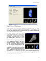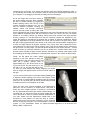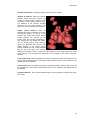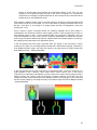
1
VolView 2.0 User’s Guide
Table Of Contents
System Overview....................................................................................................................3
Introduction .........................................................................................................................3
Free Mode Features ............................................................................................................4
Professional Mode Features .................................................................................................4
Obtaining a Trial License .....................................................................................................5
Check For Updates ..............................................................................................................6
Technical Support ...............................................................................................................6
Purchase VolView ...............................................................................................................7
Quick Tutorial .........................................................................................................................8
Step 1: Load Data ...............................................................................................................8
Step 2: Interact With Images ................................................................................................9
Step 3: Interact With The Volume ....................................................................................... 11
Loading Data........................................................................................................................ 14
Loading Data Overview...................................................................................................... 14
The Open Wizard .............................................................................................................. 16
The User Interface ................................................................................................................ 18
User Interface Overview..................................................................................................... 18
The File Menu ................................................................................................................... 20
The View Menu ................................................................................................................. 21
The Window Menu............................................................................................................. 23
The Help Menu.................................................................................................................. 24
Application Settings .............................................................................................................. 25
Interface Settings .............................................................................................................. 25
Toolbar Settings ................................................................................................................ 26
Application Area ................................................................................................................ 26
Animation ............................................................................................................................. 27
Animation Settings............................................................................................................. 27
Annotations .......................................................................................................................... 29
Volume Annotations........................................................................................................... 29
Image Annotations............................................................................................................. 33
Appearance.......................................................................................................................... 35
Volume Appearance Editor................................................................................................. 35
Bindings ............................................................................................................................... 42
Volume Mouse Bindings .................................................................................................... 42
Volume Keyboard Bindings ................................................................................................ 42
Image Mouse Bindings ...................................................................................................... 43
Image Keyboard Bindings .................................................................................................. 43
Contours .............................................................................................................................. 45
Add Contour...................................................................................................................... 45
Configure Contour ............................................................................................................. 46
Cropping .............................................................................................................................. 48
Cropping ........................................................................................................................... 48
Thick Reformat .................................................................................................................. 49
Oblique Probe ................................................................................................................... 50
Filters................................................................................................................................... 52
Filter Settings Overview ..................................................................................................... 52
Utility Filters ...................................................................................................................... 53
Surface Generation Filters ................................................................................................. 54
Edge Detection Filters........................................................................................................ 54
Segmentation - Level Sets ................................................................................................. 55
Segmentation - Region Growing......................................................................................... 56
Noise Suppression Filters .................................................................................................. 56
Intensity Transformation Filters ........................................................................................... 57
i
Table Of Contents
Image Display ...................................................................................................................... 58
Image Mapping ................................................................................................................. 58
Window / Level .................................................................................................................. 60
Lightbox Options ............................................................................................................... 61
Colors ............................................................................................................................... 62
Probe Information .............................................................................................................. 62
Information........................................................................................................................... 64
Volume Information ........................................................................................................... 64
Markers................................................................................................................................ 65
3D Cursor ......................................................................................................................... 65
3D Markers ....................................................................................................................... 65
2D Marker ......................................................................................................................... 66
Views And Lights .................................................................................................................. 67
Projection Type ................................................................................................................. 67
Standard Views ................................................................................................................. 67
Light Controls.................................................................................................................... 68
Volume Display .................................................................................................................... 69
Blending Function.............................................................................................................. 69
Super Sampling................................................................................................................. 70
Level-Of-Detail Options ...................................................................................................... 70
Colors ............................................................................................................................... 71
Saving Results ..................................................................................................................... 73
Saving Sessions ................................................................................................................ 73
Saving Volumes ................................................................................................................ 73
Saving Appearance Settings .............................................................................................. 74
Saving Surfaces ................................................................................................................ 74
Saving Screenshots........................................................................................................... 74
Edit Copy Screenshots ...................................................................................................... 75
Printing Screenshots.......................................................................................................... 75
Connect Sessions ................................................................................................................. 76
Collaboration Overview...................................................................................................... 76
Connecting And Passing Control ........................................................................................ 76
Extending Filters With Plugins ............................................................................................... 78
Extending Filters Overview................................................................................................. 78
Plugin Life Cycle ............................................................................................................ 78
The initialization function ................................................................................................ 79
The ProcessData function............................................................................................... 80
Refreshing the GUI ........................................................................................................ 82
A Detailed Skeleton Example ............................................................................................. 83
Example1: A C Filter .......................................................................................................... 86
Example 2: A C++ Filter ..................................................................................................... 88
Example 3: A VTK Filter ..................................................................................................... 91
Example 4: An ITK Filter .................................................................................................... 93
Index ................................................................................................................................... 97
ii
System Overview
Introduction
Welcome to VolView, a powerful volume visualization application intended for the medical,
scientific, and engineering communities. VolView can be used to interactively visualize, annotate,
measure, capture / print, and process volumetric and image data. New features in VolView 2.0
include:
•
•
•
•
•
•
•
•
•
•
•
•
•
•
•
Support for all data types (unsigned char
through double)
Support for up to four independent
components
Support for color/alpha, RGB, and RGBA
volumes
Over 30 basic and advanced image
processing filters
Plug-in API allows any developer to
extend filtering capabilities
Collaboration between two VolView
sessions
New interactive annotation widgets:
• Color bar, scale bar, orientation
marker
• Distance / angle measurement
• Cropping tool, 2D / 3D markers
Improved system performance and feedback
Integrated animation tool
Improved transfer function editor with more presets
Oblique probe / oblique image view
Automatic initial transfer function based on data
Improved lighting control
Redesigned user interface with customizable panels
Two modes: Professional and Free
As of version 2.0, VolView can be used in one of two modes: Free Mode or Professional Mode. In
Free Mode, VolView has all of the basic data loading, visualization, and image processing
functionality. In Professional Mode, advanced functionality such as interactive annotation,
animation, and collaboration are added. More information on these two modes is provided in the
next two sections. A trial license of VolView in Professional Mode is available, with details on how
to obtain this license provided later in this chapter.
This document is intended as both a tutorial and a reference guide. The Quick Tutorial session
will take you step-by-step through a typical VolView session including loading data, viewing
images and volumes, adding annotation, creating contours, and applying an image processing
filter. This is a good place to start if you are a new VolView user.
The remainder of this document acts as a reference guide. All users are encouraged to read the
section on The User Interface as this documents many features that are new to VolView 2.0. For
help on a particular setting on the interface you will find chapters matching the tab labels, with
3
Table Of Contents
sub sections matching the labeled frame around the interface elements. Detailed information on
each button, entry, slider and option can be found in these sections.
This documentation has been developed for VolView version 2.0. We suggest you check the
VolView home page at http://www.kitware.com/products/volview.html for any updates, news, or
frequently asked questions.
Free Mode Features
VolView 2.0 can run in one of two modes: Free Mode or Professional Mode. You may obtain a
trial license of VolView in Professional Mode once per computer. Please see the section on
Obtaining a Trial License for more information on how to do this.
If you have not yet obtained a trial license, or if your license has expired, VolView will run in Free
Mode. Although many advanced features will not be available, VolView in Free Mode is still a
powerful tool for volume visualization and image processing, providing all the functionality
necessary to perform these tasks.
When running VolView in Free Mode you will see the entire user interface, but some regions will
be "locked" indicating that the functionality is available only in Professional Mode. A small lock
icon will appear next to the label in each disabled area of the interface.
In Free Mode, the following functionality is provided:
•
•
•
•
•
•
•
•
•
•
•
Ability to load any supported data type
Appearance editor for material classification and shading
Blending functions and super sampling for volume rendering
Filters (extendable via public API)
Complex volume cropping
Control over mapping of values for image display
Interactive probing of image values
3D cursor and 3D markers
Parallel and perspective projection
Save volumes in any supported format
Save or print screenshots
Kitware would like to thank The National Library of Medicine for their part in supporting the
development of the plug-in filter capabilities. This effort resulted in the release of VolView 2.0 in
Free Mode to foster advanced segmentation and registration research in the medical and
scientific communities.
Professional Mode Features
VolView users may test the Professional Mode free during a trial period (typically 30 days), and
may purchase a license for VolView 2.0 to continue using this functionality past the trial period.
For information on obtaining a trial license, please see the next section. The last section of this
chapter provides information on purchasing a VolView license.
Professional Mode adds many advanced features to VolView 2.0. These features include:
•
•
•
4
An animation tool for basic volume / image series movies.
Interactive annotation elements including:
Dynamic header and corner text annotation
Application Settings
•
•
•
•
•
•
•
•
•
•
•
•
•
• Color bar, bounding box, scale bar
• Distance and angle measurement
• Orientation marker
Ability to customize mouse bindings
Thick reform and oblique probing
A lightbox view with up to 5x5 images
Interface for Window/Level with configurable presets
Ability to change background colors
Advanced light control for position, color, intensity
Control of perspective view angle and camera reset
Advanced level-of-detail control for volume rendering
Create multiple isovalued contours
Export volume as DICOM
Save contours in a variety of geometric formats
Save sessions and transfer functions
Collaboration mode to connect two VolView sessions
Obtaining a Trial License
The first time you run VolView 2.0 the Registration Wizard should pop up. (This may not occur if
VolView 2.0 was previously installed on this same computer.) You may access the wizard from
the Help menu on the VolView menu bar if it does not automatically appear or if you need to alter
your registration in the future. The first page of the wizard will appear as shown below.
It is highly recommended that you obtain the trial
license for VolView in professional mode in order to
experience the full power of this visualization and
data processing system. If you are connected to the
Internet, the easiest way to obtain a trial license is
to use this Registration Wizard. If you are not on
the Internet you can use this wizard to receive
instructions on alternate methods for obtaining a
trial license, and to manually install this license.
Leave the option selected to get a trial license and
click on the Next button.
On the next page you will be asked if your computer is connected to the Internet. Select Yes or
No and press Next to continue. If you selected No, then you will receive instructions on alternate
methods for obtaining a license. Your computer ID will be displayed, and you may enter this at
the registration web site: www.kitware.com/VVLicense/register.cgi or you may email this
information to [email protected]. You will receive your trial license via email, which you must
load using the file browser button.
If you indicate that your computer is connected to the Internet, then the next page in the
Registration Wizard will give you the opportunity to enter your email address. If you do enter your
email address it will be used to notify you of future releases of VolView and related products.
Kitware values your privacy and will not distribute your email address to third parties.
Once your press the Next button VolView will attempt to contact the license server and install
your license file. If this occurs successfully, you will see a message indicating this, and your trial
license will begin. Press the Finish button to close the wizard. If a connection could not be made,
you will see an error message. This may occur if your computer is not connected to the Internet,
or if you use a proxy server or VPN for your connection. If this error occurs, please use the Back
5
Table Of Contents
twice, then indicate that your computer is not connected to the Internet. You can then follow the
instructions for manually obtaining and installing a license file.
Any problems encountered during registration should be reported to Kitware technical support at
[email protected] or 1-518-371-3971.
Check For Updates
Updated versions of VolView 2.0 may be made available from time to time. If you have purchased
a VolView Professional Mode license, you will be notified via email when new updates are
available. All users running the beta version of VolView 2.0, and those who have installed
VolView from a CDROM are encouraged to check for updates.
If you are running VolView 2.0 on Windows and you have an internet connection, checking for
updates is quite easy. Simply use the Check for Updates option on the VolView20 menu under
Programs on your Start menu. Alternatively, you can start VolView and use the Check for
Updates option on the Help menu. A dialog will appear indicating either that a new version is
available (and it will list the release notes for this version) or that you are running the latest
available version.
If you do not have an internet connection, or if you are running on Linux, Unix, or Mac OSX, you
must visit the VolView web site to check for updates. The latest available version will always be
indicated on: http://www.kitware.com/products/volview.html
Technical Support
Customer support is provided free during the evaluation period and for 90 days after a license
purchase (30 days with the academic discount). Questions must be submitted via email to
[email protected], and will be answered within one business day. You may send support
questions after your evaluation period has expired, which will be answered as time permits.
When sending a question to customer support, please include the following information:
•
•
•
Your name and phone number
VolView version (use Help->About to get this information)
Mode - free, trial professional, or licensed
If you are reporting a bug, please provide
• The operating system you are using (Windows 98, Windows XP, Solaris, HP-UX, Linux,
etc.)
• The number of processors on your system
• Video card installed
• The size and type of the data you loaded (512x512x200 unsigned short data)
• A detailed description of the problem you encountered
• The sequence of operations that caused the problem, and whether it is reproducible
Kitware always welcomes customer feedback. If there is a particular feature that you would like to
see available in VolView 2.1, please send email to [email protected] with a brief description
of the functionality and how you would use it in your application area.
6
Application Settings
Purchase VolView
VolView 2.0 licenses may be purchased in the following configurations from the Kitware Online
Store.
1 license for $2500 ($1875 academic)
2 licenses for $4250 ($3200 academic)
3 licenses for $5625 ($4200 academic)
The VolView 2.0 license includes 90-day technical support (30-day for academic discount).
Please see the VolView web site at http://www.kitware.com/products/volview.html for the latest
information on licensing options and pricing.
Additional multi-license discounts, site licenses, source code licenses, and special product
customizations are also available. Please contact a Kitware representative at
[email protected] or 518-371-3971 for more information.
After you purchase VolView, you will receive email instructions indicating that you must provide
your computer ID to register the product. You can find the computer ID on the About dialog from
the Help menu on the VolView menu bar. After this information has been entered into the
licensing database (which generally takes one business day) you will need to use the Registration
Wizard to obtain your license. Select "Purchase and register the professional version" from the
initial page of the wizard, and press Next. After reviewing the instructions, press Next then
indicate whether your computer is connected to the Internet. If your computer is connected to the
Internet, you can retrieve your license easily through the wizard. If it is not, you must use the
small file icon to browse for the license file that was sent to you via email when your purchase
was completed.
7
Table Of Contents
Quick Tutorial
Step 1: Load Data
This quick tutorial will walk you through the basic steps of visualization and interacting with your
volume data. It is assumed that you will perform these steps in the order presented in this
documentation. Although some of the interface examples may look slightly different depending on
your platform (these images were captured on a Windows XP system) the tutorial concepts are
platform-independent.
In this first step we will locate and load one of the example datasets that is distributed with
VolView. Begin by selecting the Open File option on the File menu. This will pop up the file
browser as shown below. Using the controls provided by the dialog, navigate to the place where
you installed VolView. On a Windows system this will most likely be C:/Program Files/VolView20.
In this directory you will find a Data directory. In the Data directory will be a file called visfoot.vti.
Click on this file and press the Open button (or simply double click on the file to open it).
At this point the Open Wizard will pop up to
lead you through setting some of the
parameters that may not be explicitly set in
the file. For example, with this type of data
(the Visualization Toolkit XML image format)
we are missing a descriptive string for the
measured data values and the distance unit
type, and we do not have any information on
the orientation of the data during acquisition.
You will notice that values are provided in
the wizard - these come from an auxiliary
file
(visfoot.vti.vvi)
that
stores
this
information. Generally, the vvi file is written
after you have loaded a dataset so that the
information is retained for the next time you
load it. In this case, the vvi file came with
your VolView distribution. Hit the Next button twice to load the data.
This file contains the right foot from the National Library of Medicine's Visible Man dataset. This is
a CT dataset. You can view basic information about the data by selecting the Information panel
from the View menu. Also, be sure to select the 1 over 3 option from the Window menu, to see
both the volume rendering and the images at once. You interface at this point should like similar
to the image shown below.
8
Application Settings
Step 2: Interact With Images
We will now explore some of the interaction possibilities in the 2D image windows. First, we will
start by ensuring that VolView is using an RAS coordinate system for this medical data. To do
this, select the Application Settings panel from the View menu. On this panel located the
Application Area portion of the interface, and select Medical. You should see the three image
windows labeled as Axial, Frontal, and Sagittal.
Now we will switch the position of the volume
rendering and the sagittal image by selecting Sagittal
Image from the pulldown menu in the upper left
corner of the volume display window. Your display
area should now have a layout similar to the one
shown in the image on the right.
Note that each of the image display windows has a
slider along the bottom. This allows you to adjust the
currently displayed slice. In addition, a text entry box
also allows you to specify this slice. Try moving the
slider back and forth to view the slices through the
foot. There are some keyboard shortcuts as well.
Before attempting to use the keyboard shortcuts you
must ensure that this image window has keyboard
focus. If you click on the top bar of the window it will
turn blue (as it is in the image on the right) indicating
that this is the currently selected window. Now you
can use the left and right arrow keys to move back
and forward through slices one at a time. The Page Up and Page Down keys will move back and
forward by 10 slices at a time, while the Home key will go to the first slice, and the End key will go
to the last slice. Note that the slice number is reported in the text box to the right of the slider, and
in the upper left corner of the image window.
9
Table Of Contents
Move the slider back to some center position. Use the View menu to display the Image Display
panel. We will now adjust the Window and Level of the image to control the contrast and
brightness. Note that the current window and level settings are displayed both in the lower right
corner of each image window and in the Window/Level area of the Image Display panel. If you
recall on the Information panel we saw that the scalar range (the minimum and maximum value
found in the dataset) is 0 to 169, therefore the initial Window is set to 169 (to cover the whole
range) and the initial Level is set to 84.5 which is halfway between the minimum and the
maximum. We can adjust these values in one of two ways: by manually entering new values in
the Window and Level text entry boxes, or by dragging the left mouse in the image display
window. We will first start by manually entering values that will highlight the bone. Moving the
mouse over the image and looking at either the status bar at the bottom of the application, or the
Probe Information area on the Image Display panel, you can see that the scalar values in the
bone region are generally at or above 77. We will emphasize
this region by setting the Level to 77 and the Window to 50.
Making this change should alter your image to something like
the one shown on the right. Note that the other two image
windows also change due to the new window and level
settings. These values are set for the entire application
window, not per image window, keeping all 2D views of the
data synchronized.
Now try adjusting the window and level values using the
mouse. Press the left mouse button and move the cursor left
to right to adjust the window value, and up and down to adjust
the level value. You can press the Reset button in the
Window/Level area of the Image Display panel to reset these
value. In addition, the "r" key will reset both the window/level values and the display position of
the image.
In addition to the window/level functionality on the left mouse button, VolView provides panning
and zooming on the middle and right mouse buttons. To see a list of these binding, view the
Bindings panel. In the Image Mouse Bindings area you will see a grid of configurable mouse
binding for the left, middle, and right mouse buttons pressed alone, or in conjunction with the shift
or the control keys. Below this in the Image Keyboard Bindings area you will see a list of the
keyboard shortcuts including those mentioned in this section.
Spend some time panning and zooming the image to become comfortable with this functionality.
Note that when you zoom, the other image windows zoom as well. Panning occurs independently
in each image window.
Finally, let's discuss the Image Mapping area on the Image
Display panel. The current mapping is set to Raw Scalars,
and hence you are viewing the scalar values with a
window/level applied. Two other mappings are possible with
this data type: Color Mapped Scalars and Color Mapped
Scalars - Opacity Modulated. Change the Mapping to Color
Mapped Scalars. At this point it is also useful to press the
Reset button in the Window/Level area. You should now have
an image that looks like the one shown on the right. To
understand where these colors come from you will need to
open the Appearance panel. Look at the area labeled Scalar
Color Mapping. You will see that a rainbow colormap has
been applied to the data. This color mapping will be used for volume rendering, and will be used
to display the images when the Image Mapper is set to a color mapped mode. In this Image
Mapping mode we are mapping the scalar value through the color map, then applying a
window/level operation to the resulting color. If you click on a node in this area you can slide it left
10
Application Settings
or right. When you release it you will see the image window update (and the volume window)
update for the new color mapping. After clicking on a node you can also change its color by
clicking on a new color in the color wheel.
If you return to the Image Display panel (this should be in the
set of tabs at the top of the left panel area - simply click on
this tab rather than selecting the panel from the View menu)
you can change the Image Mapping to Color Mapped Scalar Opacity Modulated. Again, use the Reset button to reset the
window/level values. You should now see an image similar to
the one shown on the right. In this mapping mode, the scalar
values are mapped through the colormap, but the
window/level is applied to the original scalar value. The result
of this window/level (a value between 0 and 1) is multiplied by
the color. This tends to produce saturated colors in areas of
high image intensity, and black values in areas of low image
intensity.
Step 3: Interact With The
Volume
Now we will focus on interaction in the
volume display window. At this point you
should switch back the position of the
Sagittal image and the volume display. You
can do this by selecting Volume from the
pulldown menu in the large display area that
is currently assigned to a Sagittal Image.
The Volume window should appear similar to
the one shown on the right.
Note that the volume display window
contains both the pulldown on the left for
selecting window type, but also a progress
gauge on the right. This progress gauge is
used during rendering to show the progress
of the displayed image. In the example we
see a progress bar with three distinct
regions: one drawn in dark blue, another in
light blue, and one in green. The blue color
indicates the levels-of-detail that are drawn using a hardware-accelerated approach. The green
color indicates the level-of-detail that is drawn using a ray casting technique. This example was
run on a system with a GeForce 3 graphics board, allowing for hardware acceleration. If your
progress bar shown only shades of green, then your system does not support hardware
acceleration for the data type you have loaded.
The most common interaction methods in the volume display window are rotation, panning, and
zooming. These have been mapped to the left, middle, and right mouse buttons respectively. Try
now to interact with the volume using the mouse. If you lose the volume during this interaction,
press the "r" key (verifying first that the volume display window has keyboard focus) to reset the
camera. You can also set the camera to one of the six standard directions using the Views &
Lights panel. You may also wish to try switching between parallel and perspective projections
11
Table Of Contents
(also available on the Views & Lights panel) to see the difference between these two projection
modes.
Return now to the Appearance panel. We will
now adjust the color and opacity mappings to
alter the appearance of our rendered volume
We will first begin with turning the Gradient
Opacity Mapping on. This is done by using the
first pulldown menu area to change the Off to
On. Now, grab the second black node from the
left, and drag this node down to the bottom of the editing region. The interface should now look
something like the image shown on the right, with the volume display window appearance similar
to the image shown below it.
Here is what happens when you enable this mapping. At each location in the volume we have
computed a gradient direction, and a gradient magnitude. This mapping will assign a value
between 0 and 1 to each gradient magnitude. This mapping is a simple ramp - the mapping from
the first node to the second will be a constant value (usually you want this to be zero but you can
increase this by moving the first node up). The
mapping from the second to third node is a linear
ramp, and all values past the third node will be
mapped to 1.0. After we look up the opacity at a
sample point based on scalar value (using the Scalar
Opacity Mapping function) we then multiple this
opacity by the modulation value obtained from the
Gradient Opacity Mapping function. By eliminating
samples with low gradient magnitude values from the
image, we are effectively doing an edge detection
operation during rendering. This dataset was
obtained by CT, which tends to produce data with
sharp transitions between air and soft tissue, and soft
tissue and bone. You can see in the image on the
right that the nearly constant valued region between
the skin and the bone is eliminated due to the low
gradient magnitudes in the area. Spend some time
adjusting the gradient opacity mapping, and turning it
on and off, to get a good idea of how this mapping
will affect your image.
Now we will adjust the color settings. Start by
selecting the folder icon in the Scalar Color Mapping
area. Select the White option to set the color to solid white. Now click in the center of the editing
area for the scalar color mapping to add a new white node. Click on the first node on the left in
order to select this node. Adjust the color of this node to light brown by using the Value and Hue /
Saturation areas at the top of the Volume Appearance Settings area. Clicking somewhere in the
Hue / Saturation circle will change the color of the selected node. Alternatively, if there is a
particular Hue, Saturation, and Value that you would like, you can manually specify this in the H,
S, and V text entry boxes. Using the first pulldown in the Scalar Color Mapping area you can
change from HSV to RGB so that you may enter these values as red, green, and blue
components instead.
Now you should have one light brown node to the far left, a white node in the middle, and a white
node on the far right. Click on the line very close to the light brown node to add a second light
brown node. You will now drag this (node #2) to the right until the scalar value (the first text box
labeled S above) is approximately 45. Drag the next white node (node #3) until the scalar value is
approximately 50. The interface in the Scalar Color Mapping area should appear similar to the
12
Application Settings
example shown on the right. If not, adjust your interface until it has a similar appearance. Note - if
you accidentally add a node you can delete it either by selecting it and pressing the Delete key on
your keyboard, or by dragging it far below the editing area and releasing it.
So far the images we have been viewing in
the volume display area have been unshaded.
We will now enable shading by toggling the
Enable Shading button near the top of the
Volume Appearance Settings area. You can
edit the material properties including the
ambient, diffuse, and specular coefficients,
and the specular power by hitting the small
sphere (representing the current shading parameters) next to the Edit material label. This will pop
up the Material Properties editor with four sliders for these four values, plus four convenient
presets for no shading, diffuse only shading, diffuse with some specular, and highly specular
shading. Ambient is a non-directional term that will uniformly increase the brightness in the
image. No shading is equivalent to full ambient with no diffuse or specular contributions. Diffuse
lighting is dependent on the angle between the normal and the vector to the light source. When
the light is shining perpendicular to the surface, it will receive the most illumination, dropping off to
0 when the angle reaches 90 degrees. Specular is the "shiny" term and is dependent on the
normal direction, the light vector and the viewing vector. This can be thought of as a reflection of
the light source in a shiny object. The specular power adjusts the focus of this reflection - a small
power will mean an unfocused reflection such as you would see in brushed metal, while a high
specular power indicates a highly focused reflection indicative of a polished metal. Spend some
time adjusting the shading parameters to understand their impact on the volume rendered image.
Finally, we will adjust the scalar opacity
mapping. In this case, attempt to match the
example image to the right, noting that the first
node has a (scalar, opacity) value of
approximately (0,0), the second node is (32,
0), the third is (35, .28), the fourth is (54, .28),
the fifth is (70, .5), and the last node is (255,
.5). Once you have adjusted the opacity mapping, you should
have an image that appears similar to the one shown below on
the right.
You can use the Scale slider in the Scalar Opacity Mapping area
to adjust the whole mapping to be more or less opaque. There
are also a set of preset mappings available under the small file
folder icon. One of these (the one used by default when the data
is loaded) is based on the histogram of the data.
There are many more features available on this Appearance
panel than can be covered in a simple tutorial. This panel is
clearly the most complex interface in VolView 2.0, and defines
the core parameters that affect the volume rendered image. It is
important that you spend some time becoming familiar with the
use of this panel in order to produce effective visualizations of
your data. Please read the Appearance chapter later in the
document for more details. You may also wish to consult a
textbook that covers basic volume rendering if you are unfamiliar
with the underlying principals. One recommendation would be
chapter 7 in The Visualization Toolkit: An Object-Orientated Approarch to 3D Graphics (3rd
Edition) ISBN 1-930934-07-6.
13
Table Of Contents
Loading Data
Loading Data Overview
Using the Open File option on the File menu, you can load volumetric data as well as previously
saved sessions and appearance settings files. The dialog that opens when you select this option
is dependent on the operating system. For Windows XP, the dialog will appear similar to the one
shown below.
To load a session file, select the VolView
Session option from the Files of type menu.
Use the Open File dialog to browse your disk
for the specific file. Press Open or double
click on the session file name to load it. If the
data referenced inside the session file cannot
be found automatically, another dialog will
appear asking you to locate this file. A
session file is saved using the Save Session
option on the File menu. These files contain
all the parameters of VolView, and a pointer
to the data (the session file itself does not
contain the data).
To load an appearance settings file, select
the VolView Appearance Settings option from
the Files of type menu, find the file using the Open File browser, and press the Open button. An
appearance settings file contains the parameters from the Appearance panel. You can save
these parameters using the Save Appearance Settings option on the File menu. It is often useful
to save an appearance file when you must process multiple files of the same type in a similar
way. For example, if you are analyzing a set of CT scans of the lungs, you may find that the color
and opacity mappings for one lung dataset work well for the entire set.
VolView supports both 3D (volume) and 2D (series of images) data sets in a variety of formats as
shown below. Since these data files do not contain all the information that may be necessary for
accurate visualization, a wizard will open to guide you through setting these values. The next
section will cover the wizard in more detail.
In order to load a 3D data file, simply locate it using the Open File browser, press Open, then
follow the instructions on the wizard. To open a series of 2D data files, locate any one of the files
from the series and press Open. VolView should automatically detect the entire set of images in
the series, provided that they all reside in the same directory, they all have the same basic
parameters (such as width and height) and they follow some simple naming pattern (such as
image.1.tif, image.2.tif, etc.).
VolView supports volume that have a data type of signed or unsigned char, short, or int, as well
as float or double. These files could have 1 to 4 components per sample point. For two
component data, this can be either two independent components, or the first component could be
used to define color while the second is used to define opacity. For three component data, these
can be three independent components or RGB. For four component data, these can either be
four independent components, or RGBA. For three or four component data that is not
independent, the data type must be unsigned char. Not all file formats support all these types of
data.
14
Application Settings
The supported 2D and 3D data file formats are:
DICOM: DICOM data is generated by many medical scanning devices. VolView can not
read all DICOM files. For example, if the scanning parameters (such as field of view) were
changed during the scan, VolView will be unable to read the data. If the gantry was tilted
during scanning, VolView will be unable to read the data.
GE Signa: GE Signa data is created by some General Electric CT and MR scanners, and
will typically have a .mr or .ct extension.
BioRad Confocal: These files are created from a BioRad confocal microscope, and will
typically have a .pic extension.
Zeiss LSM: These files are created from the Zeiss microscope and typically have a .lsm
extension.
Metamorph Stack: Metamorph Stack files are the output type produced by MetaMorph
and the MetaMorph Imaging Series applications. These files are a derivative of the TIFF
format, and typically have a .stk extension.
Analyze: Analyze files are created from the Analyze volume visualization application and
will typically have a .hdr extension.
Visualization Toolkit:
VTK: VolView can read files written by the Visualization Toolkit. This includes image data
stored in the older *.vtk format, as well as the newer *.vti format.
VolVis: VolVis files are created from the VolVis volume visualization application and will
typically have a .slc extension.
BMP Images: A series of Windows bitmap files can be read to form a volume. The
extension is typically .bmp.
JPEG Images: VolView can read a series of jpeg image files to form a volume. The
extension is typically .jpg or .jpeg.
PNG Images: A series of PNG files can be read to form a volume. The extension is
typically .png.
PNM Images: VolView can read a series of pnm files to form a volume. The extension of
these files may be .pnm, .pgm, or .ppm.
TIFF Images: A series of TIFF images can be read to form a volume. The extension is
typically .tif, or .tiff.
Raw Data: Raw data files may be a series of 2D raw files or one 3D raw files. Raw files
contain a header followed by X*Y*C (or X*Y*Z*C in 3D) data values, where X, Y, and Z are
the dimensions of the data, and C is the number of components.
In addition to using the Open File option on the File menu to load data, you can also select a
recently viewed file from a list using the Open Recent File option on the File menu. When you
load data this way, the parameters that you entered previously on the Open File Wizard will be
retrieve, and the Open File Wizard will not be displayed. If you need to change some configurable
parameter in the Open File Wizard, you should instead use the Open File option. This option will
always display the wizard, even though the previous values could be retrieved from the auxiliary
.vvi file stored when you last opened this dataset.
15
Table Of Contents
The Open Wizard
The Open Wizard will guide you through setting parameters that could not be retrieve directly
from the data you are opening. In addition, it allows you to change some automatically
determined values. The exact appearance and configuration of this wizard will depend on the
dataset you are opening. A few examples are given here to guide you through entering the values
in this wizard. Depending on your data, you may not encounter all of these dialogs, and you may
encounter them in a different order than presented here.
When opening a series of image files, the first page displayed by the Open Wizard will appear
similar to the example shown below. In this dialog you will see the file pattern (in a C-style
notation) as well as the starting and ending image numbers. You can adjust the starting and
ending slice values in order to read only a subset of the data if desired.
Pressing the Next button will display the volume
attributes page of the wizard, shown on the right
below. Here you can adjust the origin (physical
coordinate of the lower, left, first slice sample of the
dataset) and t he spacing (distance between
neighboring samples). Depending on the type of
data or the existence of a previously (automatically)
saved *.vvi file for this dataset, there may be initial
guesses in these entry boxes, or the values may be
the default of (0,0,0) for the origin, and (1,1,1) for the
spacing.
Pressing the Next button will display the volume
units page of the wizard, shown on the right below.
Here you can adjust the name of the distance units
and the scalar value units for each component.
These labels will be used in various places on the
user interface and in the data annotation. For
example, the distance unit will be used for displaying
measurements (20.25 millimeters), and the scalar
value units will be used when probing (the value at
(17, 2, 37) is 10 degrees).
Pressing the Next button will display the volume
orientation page of the wizard, shown on the next
page. On this page you can adjust for the layout of
the data samples in the file. For example, if your
series of images represent Sagittal images instead
of the standard Axial, then you would adjust these
option menus to indicate this. The first option menu
lets you indicate which axis the image files move
along, and the order. The second option menu
allows you to specify the axis and order of the rows,
and the final option menu allows you to specify the
axis and order of the columns. If you load your data
and it appears to be upside-down, or flipped in left /
right, then you did not correctly specify the
orientation. If you are loading a series of images, at
16
Application Settings
this point you have completely specified the
parameters, and the data will be loaded when you
press Next or Finish.
If you attempt to load raw data (either a series of 2D
images or a 3D volume), you will see some
additional pages of the Open Wizard. Before
assuming that your data is of raw format, VolView
will attempt to read it with all possible readers. If the
data cannot be correctly recognized as a known
format, you will see the Open Wizard pop up,
requesting you to indicate that you wish to load raw
data as a series of 2D files, a single 3D file, or to
cancel this operation. An example of this page is
shown below. If your volume of raw data is
contained in one file, select the single 3D file option.
If your data is written with one 2D slice per file,
select the series of 2D files option. Otherwise,
cancel this operation.
Pressing the next button will display a page
requesting information about the raw file, as shown
below. On this page you will need to enter the
number of columns, rows, and slices in the file
(corresponding to the X, Y, and Z dimensions). You
will also need to specify the number of channels
(components) per sample, the data type, and (for
data types where this is necessary) the byte
ordering. On the right side of the page you will see
an image from the volume that will change as you
alter the settings on this page. This will help you
determine if you have set all the parameters
correctly. If the image appears skewed you have
most likely entered the columns or rows incorrectly.
The image on the right is interactive - you can use
the left mouse button to adjust window and level, the
middle mouse button to pan, and the right mouse
button to zoom. Pressing the "r" key will reset the
window / level and viewing parameters.
When loading multiple component data (more than
one channel at each sample), you will see a page in
the Open Wizard asking you whether or not the
channels are independent. If these channels
sampled
independent
properties
such
as
temperature and velocity, then the answer should be
yes. If these channels together form either an
Intensity Alpha pair, RGB, or RGBA (for two, three,
or four components respectively) then the answer
should be no and you should not check this box. The
dialog will appear similar to the one shown on the
right.
17
Table Of Contents
The User Interface
User Interface Overview
The VolView user interface consists of six main regions as illustrated below. This includes the
Main Menu Bar, the Toolbar, the Property Panels, the Display Windows, the Status Bar, and the
Main Progress Gauge. Note that not all of these regions will be visible at all times. A detailed
description of each of these regions is provided below.
Main Menu Bar: The menu bar provides pulldown menus along the top of the application
under the following headings: File, Edit, View, Window, and Help. The Edit menu may not
be available on all platforms. The File menu provides functionality for loading and saving
data, printing, connecting to another VolView session, and exiting. The functionality found
in the File, View, Window, and Help menus is described in the next sections. Information
on the edit/copy functionality provided in the Edit menu can be found in the Saving Results
chapter.
Toolbar: The toolbar is an optional interface area directly below the main menu bar that
displays pictorial representations of the different available window configurations. Clicking
on one of these buttons will change the set of windows in the display area. The visibility
and appearance of this toolbar can be controlled using the Toolbar Settings area in the
Application Settings panel.
18
Application Settings
Property Panels: The property panels are located on the left side of the window, and may
or may not be visible. You can toggle the visibility of these panels by Hide/Show Left Panel
item in the Window menu. You can control which panel is currently visible by selecting it
from the View menu. Depending on your settings on the Application Settings panel,
multiple panels may be displayed as tabs along the top of the property panels area. These
will be the most recently viewed property sheets. To switch between these panels, simply
click on the panel tab. Moving the mouse to the right edge of the panel area will change
the mouse to a horizontal double arrow indicating that you can resize the left panel area.
There is a minimum size below which you cannot resize so that interface elements will fit
on the panel. If you have an unusually large font you may find the need to increase the
size of the panel area.
There are several interesting features of the property panels. First, you can lock a property
panel in place by first clicking on the tab to make it visible (if it is not already) and then
double clicking on the tab for this panel. You will see the name of the panel change to
italics, indicating that it is locked on the property panels area. When switching between
panels using the View menu, only the unlocked panels will be swapped out for the new
panels. If you lock all of your panels you will not be able to view any new ones until you
unlock at least one.
Another interesting feature of the property panels is that you can close and open the areas
on the panel using the small icon in the corner of the area. When the area is open, the icon
will appear like a small "X". Pressing this will close the area, displaying only the area title.
The icon in the corner will now be a small downward-facing triangle. Pressing this will once
again open an area.
The areas on the panels can also be repositioned. To move an area with one panel, press
the left mouse down over the title of the area, drag it to a new position (up or down), and
release the mouse. Generally you should release the mouse over another area, and the
one you were dragging will then move below the one over which you released it. To move
an area to another panel, you would drop the area onto the tab for the other panel (both
panels must be tabs in the property panels area).
Display Windows: From one to six display windows may be visible at any time. These will
be located below the main menu bar and the toolbar, and above the status bar and the
main progress gauge. If the property panels are visible, they will be to the left and the
display windows will be to the right.
There are ten basic configurations that are displayed on the toolbar pictorially, and these
options are duplicated in the Window menu. Selecting one of these options from the
toolbar or the Window menu will alter the arrangement of windows in the display area.
There are six different types of windows as described below:
Volume: This is a volume rendering display of the data. This window supports 3D
interaction.
Lightbox: This is an image display, allowing for up to 25 consecutive images to be
displayed in a grid pattern. This window supports 2D interaction.
Oblique Probe: This is the image obtained from applying an oblique probe to the
volume displayed in the Volume window. You can turn on the oblique probe from
the Cropping panel, and adjust the placement interactively in the Volume window.
This window supports 2D interaction.
19
Table Of Contents
X-Y (Axial) Image: This is an axis-aligned slice of the data along the Z axis. This
window supports 2D interaction.
X-Z (Frontal) Image: This is an axis-aligned slice of the data along the Y axis. This
window supports 2D interaction.
Y-Z (Sagittal) Image: This is an axis-aligned slice of the data along the X axis. This
window supports 2D interaction.
For each of the display windows, there is a pulldown menu in the upper left corner (on the
title bar). Using this menu you can change the type of display in this area. For example,
selecting the first Window layout option on the Window menu or the toolbar will display one
Volume window. Using the pulldown menu you can change this to view the Axial image in
this area instead. Keep in mind that you can only display each type of window once - if you
choose a window type that is already displayed, the two windows will swap positions. For
example, if you are viewing the Axial and Sagittal image side-by-side, and you select
Sagittal from the pulldown menu on the Axial window, then the Axis and Sagittal windows
will swap positions.
Clicking on the title bar of a window will change this title bar to blue, indicating that this
window currently has keyboard focus. This is useful when using keyboard shortcuts.
Status Bar: The status bar in on the bottom left of the application. Short messages will
appear in the areas, generally when VolView is performing some complex processing, or
when the mouse is moved over an image window.
Main Progress Gauge: The main application progress gauge is on the bottom right of
VolView. During complex processing, progress will be displayed in this area as a blue bar.
Progress for rendering will be displayed on the right side of the title bar of the volume
display window.
The File Menu
The File menu contains options that allow you to load and save data, print, connect to another
VolView session, close the window and exit the application. Each of the options are described in
more detail below.
Open File: This menu option will pop up the Open dialog. More information on using the
Open dialog can be found in the chapter on Loading Data.
Open Recent File: A list of recently opened files will be displayed, allowing you to quickly
load one of these datasets. If you load a file from this list, you will not be prompted for
information such as the name of the units, the spacing and origin of the data, and the
acquisition order. If you need to re-enter this information, use the Open option to load the
file.
Save Session: This menu option allows you to save the state of your VolView session so
that you may open this again at a later time or share this with a colleague. A session
includes all of the interface settings as well as a reference to the data. For more
information about saving sessions, please see the Saving Results chapter.
Save Appearance Settings: You can save a file with the settings from the Appearance
property sheet so that you may load this at a future time. This includes the functions
20
Application Settings
mapping scalar value to color and opacity, the function mapping gradient magnitude to
opacity, the weighting values for datasets with more than one component, and the shading
parameters. These files will have an extension of .vvt and can be loaded using the Open
dialog. For more information on saving appearance settings, please refer to the Saving
Results chapter.
Save Volume: If you have modified the volume through a filtering operation, or if you
would like to change the format of your volume (for example from DICOM to a series of
jpeg files) you can use the Save Volume feature. For more information on this feature, see
the Saving Results chapter.
Save Screenshot: This option will capture an image of all the display area, and save this
image to a file on your disk. This image will include the image from each of the display
windows in the same configuration as seen on the screen. For more information on this
functionality, see the chapter on Saving Results.
Save Surfaces: If you have created a surface either through a contouring operation from
the Contours panel, or through a filter, you can save this surface using this option. All
surfaces will be saved into a single file, and you can select from Stereo Lithography (STL)
format or VTK format. Please see the Saving Results chapter for more information.
Export DICOM: If you loaded DICOM data originally, and have modified it with a filter,
then you can export this data back out as DICOM using this option. For more information
see the chapter on Saving Results.
Connect to Remote: You can connect your VolView session to another VolView session
on a different machine using this option. This will allow you to pass control back and forth
between the two session, while keeping the vi sualization linked in order to facilitate
communication between researchers located in remote locations. For more information on
this functionality, please see the Connect Sessions chapter.
Print: On Windows, the Print option will open the standard system print dialog, allowing
you to print your image to any available printer. The image will be similar to the one saved
in the Save Screenshot option in that it will be a representation of what you see on your
screen. For more information on Printing please see the Saving Results chapter.
Page Setup: The Page Setup option allows you to select a DPI (dots per inch) setting for
the printed image. The higher the DPI the better quality the image will have but the longer
it will take to generate. For further information please see the Saving Results chapter.
Close: If you have only one VolView application window open, this option will behave the
same as the Exit option. Otherwise, the close option will close only this application window.
Other VolView application windows that were launched using the New Window option
under this Window menu will remain open.
Exit: This option will exit this VolView session and any other VolView application windows
that were launched using the New Window option under the Window menu. If you have
selected to confirm your exit on the Application Settings panel then a dialog will appear
asking if you really want to exit. Otherwise the application will close with no confirmation.
The View Menu
The View menu contains eighteen entries that can be used to control the panel displayed on the
left side of the interface. These various panels contain the most of the controls for VolView
including the interface for adjusting the appearance of the volume and images, viewing data
21
Table Of Contents
properties, creating animations, adding data annotations, and filtering the dataset. Each of the
eighteen areas are described in more detail below, and you can find a chapter in this
documentation for each panel.
Application Settings: This panel provides controls for adjusting the appearance and
behavior of the application. This includes configuration items such as whether the splash
screen is shown at startup, whether the layout toolbar is visible, and the application area.
Animation: The Animation panel allows you to generate AVI files of basic rotations in the
Volume display window, or a sequence of slices in an image window.
Annotations: This panel contains a set of annotation elements for the volume and image
display windows. These include bounding boxes, text annotation, orientation markers, a
3D cursor, and distance and angle measurement tools.
Bindings: The Bindings panel allows you to view the keyboard shortcuts, and view and
modify the mouse bindings associated with interaction in the image and volume windows.
For example, if you prefer to rotate using the right mouse button instead of the left (which
is the default), you can make this change on the Bindings panel.
Contours: On this panel you can create isovalue contours. These contours will be
displayed in the volume and image windows. In addition, you can adjust properties of the
contour including color and shading parameters, and you can perform basic surface area
and volume measurements.
Cropping: The Cropping panel allows you to create complex axis-aligned crops of the
volume. It also provides a thick reformat functionality (thick oblique resections of the
volume), and an oblique probe (thin cross sections with arbitrary orientation).
Filters: This panel provides access to the plugin filters. Over 30 are provided with VolView
including basic utility filters such as thresholding and gradient magnitude, as well as more
complex ones such as techniques for level sets, noise suppression, and region growing.
New filters can be created using a publicly available API, which can then be loaded at runtime into VolView. For more information see both the Filters chapter and the chapter on
Extending Filters With Plugins.
Image Display: The Image Display panel provides the basic controls for adjusting the
appearance of the image. This includes a mapping function for displaying scalar values,
window/level controls, and probe information. This panel also contains configuration
controls for the lightbox, and a background color selector.
Information: The basic properties of the dataset are displayed on this panel including the
number of samples along each axis, the physical size and origin of the dataset, the data
type and number of components.
Markers: The Markers panel includes controls for displaying and setting the properties of
the 3 types of markers available in VolView. This includes a 3D cursor, a set of 3D
markers, and a 2D marker.
Appearance: The functionality available on the Appearance panel represents the main
properties that control the appearance of the volume rendered image. This includes the
shading parameters, weighting of the various components, and the functions that map
scalar value to color and opacity.
Views And Lights: This panel provides control over viewing and lighting parameters,
including a set of standard viewing positions, the ability to choose between parallel and
22
Application Settings
perspective rendering, and controls for adjusting the position, color, and intensity of the
light source.
Volume Display: The Volume Display panel provides some basic controls that affect the
display of the volume. This includes the blending function used during rendering, the
sampling rate used for rendering, the background color of the volume display window, and
controls for adjusting the level-of-detail rendering method.
The Window Menu
The Window menu allows you to control the appearance of the application window, and to create
a new VolView window. The appearance controls include the ability to show/hide the left panel,
and a set of standard layout options for the display windows. Note that these layout options, in
order from top to bottom, match the layout options on the layout toolbar in order from left to right.
You can create custom layouts by beginning with one of these standard options, then using the
pulldown menu on the left side of the title bar of a display window to adjust the type of window.
Each of the menu items is described in more detail below.
Hide / Show Left Panel: This option will toggle the visibility of the left panel. If you hide
the left panel, then choose a panel to display from the View menu, this panel will once
again be shown.
1 (volume): The entire display area is filled with a volume display window.
1 (lightbox): The entire display area is filled with a lightbox.
1 over 3: The display area is divided so that one volume display window is over 3 image
window. The three image images will be the X-Y (Axial) Image window, the X-Z (Frontal)
Image window, and the Y-Z (Sagittal) image window from left to right.
2 over 2: The same four windows will be displayed as in the above option, but in a 2x2
grid of windows. The volume will be on the top left, with the X-Y (Axial) Image window on
the top right, the X-Z (Frontal) on the bottom left, and the Y-Z (Sagittal) on the bottom right.
1 over 1: Two display windows will be arranged one on top of the other, with the top
window being a volume display and the bottom being an X-Y (Axial) Image window.
1 beside 1: Two display windows will be arranged one next to the other, with the left
window being a lightbox and the right window being an X-Y (Axial) Image window.
1 over 2: This layout has a volume window on the top, with an X-Y (Axial) Image window
on the bottom left and an X-Z (Frontal) Image window on the bottom right.
1 beside 2: This layout has a lightbox window on the left, with an X-Y (Axial) Image
window on the top right and an X-Z (Frontal) Image window on the bottom right.
2 over 3: Five windows are display with two on top (the volume on the left and the lightbox
on the right) and three on the bottom (the three Image windows in the same configuration
as the 1 over 3 layout).
3 over 3: This layout is similar to the 2 over 3 layout, but now three windows are on the
top: the volume on the left, the lightbox in the middle, and the oblique probe window on the
right.
New Window: This option will open a new VolView application window.
23
Table Of Contents
The Help Menu
The Help menu provides access to this documentation, information about the version of VolView,
functionality for checking for updates of VolView, and access to the registration wizard. Each of
these options are described in more detail below.
OnLine Help: Selecting this option will display this documentation. If you are on windows
this will be displayed as a compiled help file in the standard help browser. On other
systems this will display in html format in a web browser.
Check For Updates: The Check For Updates option duplicates the functionality provided
by the menu item of the same name under the Start->Programs->VolView20 system
menu. This option is available only on Windows platforms. Use this option only if you have
a network connection. This will check the Kitware web site for a more recent version of
VolView than the one you are currently using. If a newer version is found, a wizard will
appear to lead you through the download / install process. Before beginning the
installation, you should exit the current session of VolView (and any other sessions you
may have running on your system). If you do not, then you will need to reboot in order for
the new version to complete the installation.
Register: Selecting this option will display the registration wizard. You should use this
wizard if you are obtaining a trial license of VolView 2.0 in Professional Mode, or if you
have purchased VolView and you wish to obtain your license.
About VolView: This menu option will pop up a dialog containing information about the version of
VolView you are running, and contact information for reaching Kitware. In addition, your computer
ID will be displayed on this dialog (as well as on the registration dialog). You may need this
information in order to purchase VolView.
24
Application Settings
Application Settings
Interface Settings
The Interface Settings area of the Application
Settings panel contains a set of check boxes
controlling the basic behavior of the
application, and will appear similar to the
example shown on the right. These settings
are retained across sessions of VolView. The
individual items are described in more detail
below.
Confirm on exit: When this box is checked, VolView will display a dialog box requiring
you to confirm or cancel the operation when you exit VolView. If this box is not checked,
then exiting VolView will cause the application to close with no opportunity to cancel the
operation.
Save window geometry on exit: When checked, VolView will save the width, height, and
position of the VolView application. When restarting VolView, it will appear with the same
geometry as when it was last run. If this box is not checked then the default size and
position are used.
Show splash screen: The splash screen showing startup progress will be displayed when
VolView is launched if this button is checked. Otherwise, the splash screen will not be
displayed, and the application will appear once all initialization is complete. This may
require several seconds from the time you double click on the VolView icon, depending on
the speed of your computer and your current VolView configuration.
Show tooltips: When the mouse cursor is held still over a user interface element for a few
seconds, a small yellow pop-up will appear with a short usage message. If this box is not
checked, then this functionality will be disabled.
Show most recent panels: If this box is checked, then up to four recently accessed
panels will be available as tabs in the left panel. When this box is not checked, only the
current panel and any locked panels will be displayed.
Enable Interface Drag & Drop: Each area on the user interface (such as this Interface
Settings area) can be repositioned, either on the same panel or on another panel. To do
this, you simply click the left mouse over the title of the area and drag it to the new
location. To move the area to a new panel, be sure that both panels are displayed as tabs
(make sure the Show most recent panels option is enabled), and drop the area onto the
tab of the new panel. If you disable this option, you will not be able to reposition the
interface areas.
Reset Interface: If you would like to revert all areas back to their default positions
(removing the effect of all drag and drop operations on the interface), press this button.
This option is useful when you wish to only move some areas temporarily, but do not wish
for this change to persists. Otherwise, moving an interface area to a new position will be a
persistent change saved across sessions of VolView.
25
Table Of Contents
Toolbar Settings
The Toolbar Settings area of the Application
Settings panel allows you to enable or
disable the toolbar for window layout, and to
control the appearance of this toolbar. The
upper image on the right represents the
Toolbar Settings user interface, while the
image on the bottom shows the window layout toolbar which appears below the main menu bar
when enabled. Each of the three check boxes is described in more detail below.
Flat frame: Checking this option will remove
the raised frame around the toolbar.
Flat buttons: Checking this option will remove the raised frame around each of the
buttons in the toolbar.
Show window layout toolbar: The toolbar will be displayed when this box is checked,
otherwise it will be hidden. This toolbar duplicates functionality available on the Window
menu, and therefore is optional. Pressing a button in the toolbar will cause the display
windows to be arranged as shown. The buttons from left to right on the toolbar correspond
to the options from top to bottom on the Window menu.
Application Area
The Application Area user interface on the
Application Settings panel allows VolView to
be tailored for a specific application area.
The interface will appear as shown in the
image on the right.
There are two options for the application area: general or medical. When a general application
area is selected, VolView will display the data within an XYZ coordinate system. These X, Y, and
Z labels will be used throughout the display area and the user interface for annotation, labels,
tooltips, etc. When a medical application area is selected, VolView will use a standard RAS
coordinate system (right, anterior, superior) for displaying the data. The labels Right (R), Left (L),
Anterior (A), Posterior (P), Superior (S), and Inferior (I) are then used for annotation and user
interface.
If you load a dataset which is known to be medical in nature (DICOM or GESigna format, for
example), then VolView will automatically set the application area to medical. VolView will not
change the application area back to general, this must be manually done using this interface.
26
Animation
Animation Settings
The Animation Settings area is the only area
on the Animation panel. The appearance of
this panel will depend on whether the
Animation type option is set to 3D View or
Slices. Both examples are shown in this
section.
Using the Animation Settings area you can
create an AVI file that either shown a simple
rotate/zoom animation of the volume display
window, or a sequence of slices in one of the
X-Y (Axial), X-Z (Frontal), or Y-Z (Sagittal)
image windows. The common controls are
described below, followed by those that are
specific to each animation type.
The common interface elements are:
Number of frames: This value
specifies the number of frames in the output animation. Smaller numbers will lead to faster
animation creation times, but a jumpier appearance. Larger numbers will provide a smooth
appearance, but may take a while to generate and may produce large AVI files (depending
on compression type).
Animation type: The animation type can be set to either 3D View or Slices. With 3D View
you can specify rotation and zoom factors to be applied across the animation sequence.
For Slices you can loop through the slices in one of the three primary directions.
Preview: The preview button will allow you to view the animation in the volume or image
window. For 3D View animations, an interactive volume rendering rate will be used for the
preview, while a higher quality rendering will be used when the animation is created.
Create: The create button will pop up a Save
Animation dialog allowing you to specify the
location and file name of your animation. The file
type will be AVI and therefore the animation file
will have an avi extension. This will be added to
the filename if you do not enter it here. Once
you've selected the file name, the Video
Compression dialog will be displayed allowing you
to select a compressor type for this file. Note that
this is a standard Windows dialog (which will
appear similar to the one shown on the right) but not every compression format will be
supported by your system. Uncompressed Full Frames will always work. You may need to
experiment with a few of the compressed types to determine if it is supported by your
system, how much compression is achieved, and what the best trade-off is for image size
vs. image quality. This trade-off is controlled with the Compression Quality slider.
27
Table Of Contents
During creation, the images will be rendered into a memory buffer, and the progress of the
animation creation will be displayed on the main progress gauge in the lower right corner
of the application. This means that it is safe to close VolView or pop other windows on top
of it - this will not affect your animation. The volume rendering will be performed at the best
possible quality based on your settings in the Level-Of-Detail Options area on the Volume
Display panel.
Cancel: The cancel button can be used to cancel the preview or creation of an animation.
The interface elements specific to the 3D View animation type are:
X rotation (azimuth): Use this area to specify the total rotation about the X axis (of the
viewing coordinate system) that will occur during the animation. This is specified in
degrees, so if you want a full rotation you would enter 360.
Y rotate (elevation): This value indicates the total rotation about the viewing coordinate Y
axis that will occur during the animation..
Z rotation (roll): This value specifies the roll (rotation around the viewing coordinate Z
axis) that will occur during the animation.
Zoom factor: The zoom factor is a value that indicates how much you will zoom in or out
during the animation. The number should be close to 1.0 (1.0 indicates no zoom) where
values above 1.0 indicate zooming in, and values below 1.0 indicate zooming out.
The interface elements specific to the Slices
animation type are:
Slice type: This option menu can be
used to choose between the three
different major axes.
Starting slice: This value indicates
the starting slice for the animation.
Ending slice: This value indicates the
ending slice for the animation.
28
Annotations
Volume Annotations
The Volume Annotations area of the
Annotations panel provides a set of
annotation elements that can be added to
the volume display windows. An example of
this interface is shown on the right. The
seven different annotation elements are
described in more detail below.
Corner Annotation: A toggle button
is provided to turn on and off the
corner annotation. Depending on the
type of data you loaded, you may
already have corner annotation visible in your volume window. For example, when loading
some medical datasets such as DICOM, the Study and Series will be displayed in the
upper left corner, and the Patient Name, ID, and Date will be displayed in the upper right
corner.
The check button can be used to toggle the visibility of the corner annotation. Press the
Edit button directly to the right of the Display corner annotation check button in order to
control the actual text and the text properties such as font, style, and color. Pressing the
Edit button will pop up a dialog that will appear similar to the one shown on the right. In this
case we have loaded medical data and therefore some corner annotation was entered
automatically by VolView from the header information in the file. To alter the text
annotation in any of the corners simply type in the text window for that corner of the
window. The four text entry windows (which support multi-line input) are labelled for the
four corners of the volume display window: Upper left, Upper right, Lower left, and Lower
right. Below these text entry areas are a set of controls that can be used to customize the
appearance of the text. These controls are described in more detail below. These text
properties apply to all four corners of the window.
Max line height: This value will
control the height of a line of text. If
the text appears too big, decrease
this number. If it appears too small,
increase it. You can type the new
value in the text box, or use the
arrow to pop up a slider.
Depending on the number of lines
of the text and the size of your
window, it may be that only the
lower values have any significant
effect on the size of the text, since
other constraints may limit the
behavior of this slider. This option
is often useful when printing since
the size of text that is appropriate
for being able to read it on the
computer monitor may not be the
optimal size for a printout.
29
Table Of Contents
Color: This button can be used to adjust the color of the text displayed.
Family: The font family can be selected from the pulldown menu.
Style: The style of the text can be selected using these toggle buttons. You can
toggle bold, italics, and shadow. When a button appears to be pushed in, this option
is selected. Each of the three options can be toggles on and off independently.
Opacity: This value adjusts the opacity of the text. When the opacity is 1.0, the text
will be fully opaque. Choosing values less than 1.0 will cause the text to become
translucent, allowing you to see through the text.
Header Annotation: The Display header annotation
button can be used to toggle the visibility of the header
annotation. The header annotation is a string that is
displayed along the top center of the volume display
window. It is best to use the header annotation only when
the corner annotation is off, empty in the top left and top
right corners, or contains only short strings. Long text
strings in both the upper corners of the corner annotation
and the header annotation will overlap.
Press the Edit button to pop up the Volume Header
Annotation dialog. An example of this dialog is shown on
the left. Use the Header text entry box to enter the string
that you would like displayed on the volume window. The properties of the header,
including the color, font family, style, and opacity can be set. See the description above for
corner annotation for a definition of each of these properties.
An example image showing a variety of volume annotations is shown near the end of this
section. In this image you can see both corner annotation in
the upper left and right corners in yellow Arial, and header
text in the center top in white italic Times. Also shown in the
image are a bounding box, a color bar, an orientation widget
and a color bar.
Color Bar: The color bar is a graphical representation of the
color mapping that is currently applied to the scalars in the
volume window. This is an interactive annotation element.
There are aspects of the color bar that can be controlled with
the interface, such as toggling the visibility, adjusting the
labels, a setting the title. In addition, there are aspects of the
color bar that can be controlled interactively using the mouse
in the volume display window. For example, you can scale the
color bar, switch the orientation between horizontal and
vertical, and adjust the placement of the color bar in the
window.
In the example image near the end of this section you can
see a color bar oriented vertically along the right side of the
volume display window. You can toggle the visibility of the
color bar with the Display color bar toggle button. By pressing
the Edit button you will bring up the control panel for the color
bar, which will appear similar to the example shown on the
30
Annotations
right. Each of the items in this control panel will be described in more detail below.
Component: When working with multiple component data, this pulldown menu will
allow you to select the component for which you wish to view the color bar. Only
one color bar for one component can be displayed at any time.
Title: The color bar can be labeled. This title will appear along the top of the color
bar (in either vertical or horizontal mode). You can adjust the appearance of the title
using the Title properties elements below.
Title properties: Using this set of interface elements you can adjust the color, font
family, style and opacity of the title of the color bar. For a description of each of
these elements please see the documentation for the corner text annotation above.
Label text properties: You may used this set of interface elements to adjust the
text properties including color, font family, style, and opacity of the labels.
Maximum number of colors: This value adjusts the number of color segments
used to display the color bar. A smaller number will lead to a blocky appearance in
the color bar. A large number will lead to a smooth appearance of the color bar, but
may degrade performance.
Number of labels: The number of labels can be adjusted. Bringing this number
down to zero will remove all of the labels.
In addition to these user interface
elements that adjust the appearance of
the color bar, you can reposition and
resize the color bar interactively in the
volume widget. Move the mouse over
the color bar while VolView is in an idle
state (not currently rendering). You will
notice that the mouse icon changes. If
you are in the middle of the color bar
you will see a vertical double arrow
and a horizontal double arrow. This
indicates that using the left mouse
button now will allow you to draw the
color bar to a new location on the
window. If you move close to the top or
bottom edge of the window, the color
bar will switch to horizontal mode. If
you move near the left or right edges
of the window, the color bar will switch
to vertical mode. When the mouse is
near an edge of the color bar you will
see a horizontal double arrow
(indicating that you can alter the width
of the color bar), a vertical double arrow (indicating that you can resize the height of the
color bar), or a diagonal double arrow (indicating that you can do both at once).
Orientation Marker: The orientation marker is an interactive annotation element
displaying the current orientation of the data using a box with labels on the sides. In the
example image shown on the right, the Orientation marker is shown in the bottom left
corner of the volume display window. The application area is set to Medical, and therefore
31
Table Of Contents
the box uses R (right), L (left), A (anterior), P (posterior), S (superior), and I (inferior).
When in a general application area the letters would be +X, -X, +Y, -Y, +Z, and -Z.
From the user interface you can toggle the visibility of the orientation marker, and set the
color. Since the labels will always be drawn in black, selecting a light color for this
annotation element is best. In addition to the user interface control, you can also reposition
and resize the orientation marker interactively. Move the mouse cursor over this widget
when VolView is in an idle state. When the cursor becomes a vertical and horizontal
double arrow, then you can reposition the orientation marker. When the cursor becomes a
diagonal double arrow (only in the corners of region surrounding this element) then you
can resize (both height and width equally) the orientation marker.
Scale Bar: The scale bar is an interactive annotation element that shows a ruler indicating
a specific measurement on the viewing plane. This element can only be added to the
scene when the camera is in a parallel projection mode (see the Projection Type section in
Views And Lights). If you attempt to enable this annotation element while in perspective
mode, a dialog will pop up indicating that this is not possible.
The distance label shown on the scale bar will be based on the spacing on the data, the
zoom of the camera, and the unit type specified when you loaded the data. In the example
we see that the scale bar shows a distance of "100 Units". The label "Units" will be used
whenever the unit distance type is unspecified. As you zoom the camera, the scale bar will
at first zoom with the image. Once it grows or shrinks beyond a certain limit, it will jump to
a new displayed distance.
The user interface allows you to toggle the visibility of the scale bar, and to set the color of
the scale bar. If you move the mouse over the scale bar when VolView is idle, then you will
see the cursor change. When the cursor is a vertical and horizontal double arrow, then you
can move the scale bar to a new position on the window. If you move to the far left or right
edges of the scale bar area, the cursor will become a horizontal double arrow. In this mode
you can resize the width of the scale bar. This resizing will not be smooth, since an attempt
is made to keep the displayed units in multiples of as large a value as possible given the
units and the screen size. Therefore you will see the scale bar "snap" to a new size as you
drag the mouse
Bounding Box: Using the Display bounding box toggle button you can toggle the visibility
of a bounding box around the volume. Turning this bounding box on is often useful when
trying to understand the placement of some particular structure you are currently
visualizing within the whole dataset. It can also be useful when using the cropping
functionality. You can adjust the color of the bounding box. A bounding box is shown in the
annotation example image shown above on the right.
Distance Measurement: The distance measurement tool is an interactive annotation
element that allows you to measure the distance between any two points in the data.
When you enable this tool, you will see a line with two spheres at the endpoints appear
within the dataset. Also, you will see a measurement string, initially displayed in the lower
left corner of the volume display window. If you move the mouse over the distance
measurement text, you will see the horizontal and vertical double arrow indicating that you
can reposition this text. The line and spheres can be repositioned as well, although the
mouse cursor will not change when you move over these elements. You can drag either of
the two endpoints and reposition them anywhere within the dataset. You can also drag the
entire measurement tool by clicking on the line. Remember, your movement will be
constrained by the bounds of the volume
32
Annotations
Image Annotations
The Image Annotations area on the
Annotations panel contains the annotation
elements that can be displayed in the image
windows. Most of these annotation items are
identical to those available in the volume
display window. In these cases, the reader is
referred to the previous section on Volume
Annotations for further information.
An example of the Image Annotations area is shown on the right. Each of the five annotation
elements are described in more detail below. Note that the Image Annotation area affects all
image display windows in VolView.
Corner Annotation: The corner annotation for the image windows functions the same as
the corner annotation for the volume display area. Use the toggle button to turn the corner
annotation on and off. Use the Edit button to bring up the corner annotation dialog which
will allow you to set the multi-line text string to display in each corner, as well as properties
of this string such as color, font, style, and opacity. Keep in mind that corner annotation is
automatically added to the image windows when you data is loaded. The exact corner
annotation is dependent on the data type, but will always include the window and level
values in the lower right, and the image (slice) number in the upper left. If you open the
corner annotation dialog you will see these dynamic text elements already entered. These
items will be enclosed in "<" and ">". A brief description of the different dynamic annotation
elements is given below.
<window>: This will be replaced by the label "Window: " and the current window
value from the Window/Level area on the Image Display panel.
<level>: This will be replaced by the label "Level: " and the current level value from
the Window/Level area on the Image Display panel.
<image>: This will be replaced by the label "Image: " and the current slice number
from the slider at the bottom of this image display window.
<slice>: This is identical to the <image> element, except that the label will be
"Slice: ".
Header Annotation: The header annotation for the image windows functions the same as
the header annotation for the volume display window. Use the toggle button to turn on the
header annotation, and press the Edit button to bring up the header annotation dialog. This
dialog will allow you to set the string that you want displayed at the top of the window,
along with the text properties such as color, font, style, and opacity.
Scale Bar: The scale bar can be used to indicate scale using a small ruler drawn on the
image window. The scale bar in the image window behaves the same as the scale bar in
the volume window. You can use the toggle button to toggle the visibility of this element,
and you can change the color. It is an interactive element that you can reposition and
resize. Please see the Volume Annotations section for more details.
Distance Measurement: The distance measurement tool is a line with two spheres at the
endpoints. A measurement value is displayed indicating the distance between the two
endpoints. This is an interactive annotation element in that you can reposition the text
label, and you can move each endpoint or the whole measurement line. For more
33
Table Of Contents
information on the interaction with this annotation element, please see the Volume
Annotations section.
Angle Measurement: The angle measurement tool is an angle indicator (two lines with
three endpoints) and a label indicating the angle between the lines. Use the toggle button
to turn on this annotation element. You will see the two attached line segments appear on
the image, and the text label indicating angle in the lower left corner. This is an interactive
annotation element. You can reposition the text by dragging it to a new location. In
addition, you can move the entire angle measurement tool by clicking on one of the lines
and dragging it within the image. Clicking on an endpoint will adjust the position of this
point.
34
Appearance
Volume Appearance Editor
The Volume Appearance Editor is the only
area on the Appearance panel. This area
provides access to most of the parameters
that affect the volume rendering. A thorough
understanding of the functionality presented
here is recommended for creating effective
visualizations.
An example of the interface is shown on the
right. The appearance of this panel will vary
based on the type of data loaded. This
example
was
produced
with
two
(independent) component data. The controls
allow you to adjust the material properties
and color/opacity mapping per component of
your data, and adjust the weights of the
components. Each area on the interface will
be described in detail later in this section.
In volume rendering, the appearance of the
final image is heavily influenced by the
functions applied to map the data into color
and opacity. This also happens to be the
most difficult aspect of volume render since it
is data-dependent and typically must be
performed by hand.
In VolView there are three different
mappings that impact the rendering process.
The Scalar Color Mapping converts the
scalar data into RGB colors, the Scalar
Opacity Mapping converts the scalar data into alpha values (transparency), and the Gradient
Opacity Mapping converts the magnitude of the gradient (rate of change in the scalar data) into
opacities. The scalar color and opacity mapping are useful for classifying data values into
different materials, while the gradient opacity mapping is useful for enhancing edges in the data.
Each of the elements on the interface is described in detail below. Since many of the elements
are inter-dependent, it will be necessary to read through this entire section for a complete
understanding. This documentation is written with the assumption that the section will be read in
its entirety.
Component: When your data contains more than one independent component, this option
menu will allow you to switch between components. The Scalar Color Mapping, Scalar
Opacity Mapping, Gradient Opacity Mapping, as well as the shading parameters set in the
Material Properties dialog are per-component properties that must be set independently for
each component by using this option menu. The Interpolation, Enable Shading, and
Interactive Apply options as well as the Component Weights are set once for the dataset,
and there values will not change when adjusting the active component.
35
Table Of Contents
Interpolation: Two interpolation options are provided: nearest and linear. In the process of
volume rendering it is necessary to take a sample at a 3D position within the data. This
interpolation method determines how the scalar value is obtained at the desired (x,y,z)
location from the neighboring sample values. When this option is set to Nearest, a nearest
neighbor interpolation is employed, meaning that the closest sample value is used as the
value at the (x,y,z) location. When this option is set to Linear, a trilinear interpolation
method is used to approximate the value based on the eight surrounding neighbors.
Generally you will want to keep this option in the Linear mode, but in some applications,
especially with small, labeled data sets, it is useful to view the image without the
interpolation effects.
Edit material: The Edit material button
shows a representation of the current
material settings (applied to a sphere). You
can edit that material properties including
the ambient, diffuse, and specular
coefficients, and the specular power by
hitting the small sphere (representing the
current shading parameters) next to the
Edit material label. This will pop up the
Material Properties editor with four sliders
for these four values, plus four convenient
presets for no shading, diffuse only
shading, diffuse with some specular, and
highly specular shading. An example of
this interface is shown on the right.
When the Enable Shading button is off, the lighting parameters in use are equivalent to full
ambient with no diffuse or specular contributions. The values specified here are only
applicable when shading is enable.
Ambient is a non-directional term that will uniformly increase the brightness in the image.
Diffuse lighting is dependent on the angle between the normal and the vector to the light
source. When the light is shining perpendicular to the surface, it will receive the most
illumination, dropping off to 0 when the angle reaches 90 degrees. Specular is the "shiny"
term and is dependent on the normal direction, the light vector and the viewing vector. This
can be thought of as a reflection of the light source in a shiny object. The specular power
adjusts the focus of this reflection - a small power will mean an unfocused reflection such
as you would see in brushed metal, while a high specular power indicates a highly focused
reflection indicative of a polished metal.
Enable Shading: The Enable Shading button can be used to toggle shading. Shading is
enable or disabled for all components at once, although it is possible to set the material
properties for a particular component so that no shading is applied (Ambient = 1.0, Diffuse
and Specular = 0.0) even though shading has been enabled.
The first time you enable shading and the volume renders you may notice a delay while
the gradient values are calculated. If you have already enabled the Gradient Opacity
Mapping, then the gradients will have been calculated then. When the gradients are
calculated you will see a message in the status bar area, and progress will be displayed on
the main progress gauge.
Interactive Apply: The Interactive Apply toggle button can be used to control whether or
not the changes made to the mappings are displayed interactively (while the change is
made) in the volume display window. If this button is off, then the volume window will only
update after the change is made (the mouse button is released). If this button is on, then
36
Information
while you reposition a node in one of the mapping functions (by dragging the small circle)
the volume display windows will be rendering with the adjusted mapping. By default this
option is turned off, but it can be useful while editing your mappings when you have small
data or a powerful computer.
Scalar Opacity Mapping: The Scalar Opacity Mapping region allows you to control the
mapping from the scalar value in the dataset, to an opacity value used during rendering.
This function can be adjusted, for example, to give your volume a fuzzy, cloud-like
appearance or a sharp surface-like appearance.
On the right you see an example of how
this area may look. We will ex ample
each portion of this editor in detail. The
discussion of Scalar Color Mapping and
Gradient Opacity Mapping assume that
you have already read this section on
Scalar Opacity Mapping, since many of
the elements of these editors are similar.
On the top right corner of the editor you see the currently displayed scalar range. For this
data the scalar range is [0,4095], which was initially displayed by this editor. Using the bar
on the bottom of the editor you can control the range. By dragging the rectangle on the left
you can adjust the lower range value, and by dragging the rectangle on the right you can
adjust the upper range value. The full range of the adjustment bar is the scalar range of
the data (reported on the Information panel). In this example you can see that the upper
range has been reduced by moving the right rectangle to the left. You can also move the
entire bar by clicking between the rectangles and dragging it to a new position. Double
clicking on the range bar will cause it to expand to the full range of the data. Focusing in on
a smaller region of the full range can be useful when making a detailed mapping function,
although typically you should be able to specify you function while viewing the entire
range.
Below the Scalar Opacity Mapping label we have two buttons and a pop-up slider. The first
button toggles "Window / Level Mode". When this mode is enabled, the mapping will be
reduced to a basic window / level function. The function will contain only four nodes, with
the first two having the same opacity value, and the last two having the same opacity
value. A linear ramp is therefore specified between the second and third nodes. More
details on interacting with the nodes when in Window / Level Mode is provided below.
The next button (with a file icon on it) is a pulldown menu that allows you to choose a
preset opacity mapping from a list of available mappings. Two of the mappings specify
constant opacity functions (at 0.2 or 1.0), and two represent linear ramps over the whole
scalar range of the data (from 0.0 to 0.2, or from 0.0 to 1.0). The default mapping is based
on a histogram of the data (which is displayed in the node editing area), and is a linear
ramp from 0.0 to 0.2 within a reduced range of the data (computed using the histogram).
The Scale slider pop-up allows you to scale the entire opacity of the mapping. Since
opacity is not an instantaneous value, but is defined per unit length traveled through the
volume, we need to set to length over which to apply the opacity values in our mapping.
The default length will be the average spacing between your samples. Increasing this
length (using the pop-up slider) will decrease the opacity of your volume (since less
opacity will be accumulated over the same distance) while decreasing the length will
increase the overall opacity.
The rectangular editing area displays a log-based representation of the histogram of the
scalar data in the background. The piece-wise linear function defining the opacity mapping
37
Table Of Contents
is displayed as a sequence of circles and lines. Clicking on one of the circles will display
the node number (ordered left to right) and will change the color from white (inactive) to
grey (active). At this point, the (scalar,opacity) values associated with the node are
displayed in the S and O text entry areas. You can modify the values in the node either by
typing in the text areas, or by dragging the node. Moving the node left or right will decrease
or increase the scalar value, moving the node down or up will decrease or increase the
opacity value. The motion will be constrained to keep the nodes in order (node 3 must
remain between nodes 2 and 4). If you use the shift key in conjunction with the mouse, the
motion of the node will be constrained to be entirely vertical or horizontal (press the shift
key after you begin dragging either vertically or horizontally to constrain to this direction).
When a node is active, you can move to the next node by pressing the "n" or Page Down
keys on your keyboard. You can move to the previous node using the "p" or Page Up keys.
The Home key will bring you to the first node, while the End key will bring you to the last
node. Note that you cannot adjust the scalar value of the first or last nodes in the mapping
- these are fixes at the bounds of the scalar range.
To add a new node to the mapping, click the left mouse button on the location where you
want to add the node. This will become the active node, and you can adjust the values
either interactively by dragging the node, or with the text entry boxes for S and O. To
delete a node you can either drag it far below the editing box (the standard dragging icon
will change to a black box icon indicating that the node will be delete) or you can press the
Delete key or the "d" key on the keyboard when the node is active.
When in Window / Level Mode, only four nodes are displayed. No new nodes can be
added, and no nodes can be deleted. The scalar value (horizontal position) of nodes 2 and
3 can be adjusted to alter the Window and Level settings for the application. In this mode,
these settings are tied to the ones used for the display of 2D images. Adjust the Window
and Level values in one of the 2D image views will alter the scalar opacity mapping. In
addition, adjusting the position of the second and third nodes in the scalar opacity mapping
will alter the Window and Level settings used to display images. This mode can be quite
useful when attempting to focus in on a particular scalar region (for example, bone) in your
dataset. In addition to the horizontal motion of nodes 2 and 3, you can also adjust the
vertical placement (opacity). This opacity has no meaning in the image windows and will
not affect the display of the images. Typically, the first two nodes are left at an opacity
value of 0.0 (otherwise the volume image tends to become saturated) and the final two
nodes are adjusted to the desired opacity.
Scalar Color Mapping: The scalar
color mapping area is used to assign
color to each scalar value in the
dataset. This will allow you to, for
example, assign a pink color to the soft
tissue values in a dataset, while
assigning white to the bone region. An
example of this interface is shown on
the right.
When working with data with one component or independent components, the histogram
displayed in the background of the scalar color mapping will be identical to the one
displayed in the scalar opacity mapping region, since the same component is used to
derive both. When working with two component data that is not independent (it is
luminance / alpha data), the first component is used for the scalar color mapping, and the
second is used for the opacity mapping. Hence the histograms will appear different. When
working with four component data that is not independent (it is RGBA), the scalar color
mapping region will be absent, since the colors are directly obtained from the data.
38
Information
Similar to the scalar opacity mapping region, the values displayed in the upper right corner
represent the range of the data, and the range bar along the bottom of the editor can be
used to adjust the displayed range for fine editing. The active node will be larger than the
others, and will display its node number. The text entry boxes in the upper right will reflect
the scalar and color values associated with that node. The scalar value is in the first text
box marked S. The color is displayed as either hue, saturation, and value (H, S, V) or red,
green, and blue (RGB) depending of the setting of the first pulldown menu below the scalar
color mapping label. This setting (HSV vs. RGB) will also effect the color space used to
interpolate colors between nodes. In the example above the color space is set to HSV, and
you can see in the representation of the interpolated color (the color rectangle below the
editing area) that green is between yellow and blue. In RGB color space, the interpolation
from yellow to blue passes through grey.
In addition to the color space button, two other buttons are located below the scalar color
mapping label. The center button (with a lock icon on it) allows you to lock the scalar color
and scalar opacity mappings together. Nodes will be added in each function so that a
matching set (at the same scalar value) exist. When these functions are locked, horizontal
motion (changing of the scalar value) of a node in one mapping is mirrored in the other.
Adding or deleting a node will occur in both mapping, and any changes in the range
display will also be reflected in both mappings. The functions cannot be locked together
when the scalar opacity mapping is in Window Level Mode.
The right button (with a file icon on it) contains some preset color. This includes a set of
solid colors, a ramp from black to white, and two rainbow options (one that is histogram
dependent, and one that spans the full range).
Editing the nodes in the scalar color mapping is similar to
editing in the scalar opacity mapping, except that the nodes
are constrained to a line. Vertical position has no meaning.
Instead, the color of the node is set using the Value and
Hue/Saturation controls from the top of the Volume
Appearance Settings area. An example is shown to the right.
The color of the active node will be displayed in this region,
and you can adjust the Value and Hue/Saturation settings of
the current node by dragging the position of the bar (on the
Value display) and the circle (on the Hue/Saturation display).
The appearance of the Value area will be based on the current
color selected in the Hue/Saturation area. Color is always specified in HSV color space
even when an RGB color space is used to display the color value and interpolate between
color values. HSV is more natural for color definition since the spectrum of colors can be
conveniently displayed on a circle.
The scalar color mapping area support the same keyboard shortcuts as the scalar opacity
mapping area: use the "n" or Page Down keys to move to the next node, the "p" or Page
Up keys to move to the previous node, Home for the first node, End for the last node, and
the "d" or Delete keys to remove the active node. In addition, you cannot adjust the
position of the first or last nodes, nor can you delete these nodes.
Gradient Opacity Mapping: The
gradient opacity mapping area is used
to assign an opacity multiplier to
gradient magnitude values. This allows
you to reduce the impact regions with
homogenous values, and enhance the
areas of sharp change, effectively
39
Table Of Contents
performing 3D edge detection during rendering. This function is always a simple ramp with
four nodes, similar to the scalar opacity function when in Window Level Mode. An example
of the gradient opacity mapping area is shown on the right.
Similar to the other two mappings, the range of the gradient magnitude function is
displayed in the upper right corner, and the range bar at the bottom can be used to view a
subregion of this range. Regardless of the data type, this range will always be positive,
starting from zero, and will be smaller than the full scalar range. This is due to the fact that
most gradient magnitudes will have generally low values compared to the full scalar range.
Initially, the gradient opacity mapping will be Off (shown on the first button under the label)
and the histogram will be absent, as shown in the image at the beginning of this section.
You will need to turn on the gradient opacity mapping, and wait for a ray cast image to be
generated (and therefore the gradients will be computed) before the histogram of the
gradient magnitudes will be displayed. Alternatively, if you enable shading then the
gradients will be computed (the direction rather than the magnitude is needed for shading,
but both are computed at once) and the histogram will be displayed.
Note that gradients consume memory on your computer. If you have used most of the
physical memory on your computer before you have turned on either shading or the
gradient opacity mapping, then it is likely that system performance will degrade when you
turn either of these on since virtual memory will be employed.
The button with the file icon provides a few preset gradient magnitude functions. Generally
you will need to adjust this by hand since it is highly data dependent. When interacting with
the nodes you will notice that the first two are linked in opacity, and the last two are linked
in opacity (and must be 1.0). The second and third nodes can be moved horizontally to
adjust the strength of the edge detection. Generally, the first two nodes should be kept at
0.0, but occasionally there will be a need to set these to some small non-zero value in
order to de-emphasize but not entirely hide the homogeneous regions of the dataset.
On the right you will see three images generated from the same dataset. The scalar
opacity mapping for all three is the Fixed 0.2 preset option. The scalar color mapping for all
three is the White preset option. In the top image, the gradient opacity mapping is off, while
in the other two image it is on, with the first two nodes having an opacity of 0.0. This
eliminates the homogeneous regions of the data, highlighting the surfaces. The top two
images have shading off while the bottom image has shading on. Note the significant
image the gradient opacity mapping and shading can have on the volume rendered image.
Component Weights: If you have more than one independent components in your
dataset, you will see a slider for each component at the bottom of this area. These sliders
allow you to adjust the contribution of each component to both the volume rendered image
and the image display. You can see one component by itself by setting its slider to 1.0 and
all others to 0.0. If your data is in mostly separate regions (a voxel will generally have a
high opacity value in only one of the components) then setting all sliders to 1.0 would
40
Information
produce a good image of the combined data from all channels. If the data is highly
overlapping (a voxel may be highly opaque in more than one component) then using lower
values on the slider will reduce the change of oversaturating the image.
41
Table Of Contents
Bindings
Volume Mouse Bindings
The Volume Mouse Bindings area on the
Bindings panel allows you to view and adjust
the mouse bindings for the volume window.
This interface will appear similar to the
example shown on the right. A set of
adjustable operations are displayed as a grid
covering the left, middle, and right mouse
buttons pressed alone or in conjunction with
the shift or control keys. A description of
each of the possible operation choices is given below.
Rotate: Press the designated mouse/key combination in the Volume window and drag
(move the mouse without releasing the button) to rotate the volume (and any 3D
annotation). For example, mouse movement to the right will cause the volume to rotate
around to the right.
Pan: Press the designated mouse/key combination and drag to move the volume (and any
3D annotation). For example, mouse movement to the right will cause the volume to move
to the right.
Zoom: Press the designated mouse/key combination and drag to move in closer or farther
from the volume. Upward motion will zoom in, while downward motion zooms out.
Roll: Press the designated mouse/key combination and drag to roll the image. Upward
motion rolls clockwise, while downward motion rolls counter-clockwise.
Fly In: Press the designated mouse/key combination to "fly" toward the volume. You will
fly in the direction the mouse points. If the mouse is in the center this will be similar to
zooming in. If you move the mouse from the center, you will turn in the direction of the
mouse. The best way to work with this mode is to point toward the location where you want
to fly. The speed of flight is controlled by the slider at the bottom of the Volume Mouse
Operations area.
Fly Out: Press the designated mouse/key combination to fly away from the volume. This is
the same as the Fly In mode, only zooming out instead of zooming in.
Volume Keyboard Bindings
The Volume Keyboard Bindings area on the
Bindings panel displayed the keyboard
shortcuts for the volume display window. An
example of the interface is shown on the
right.
Currently the volume display window supports only one keyboard shortcut. Pressing the "r" key
while the volume display window has keyboard focus (the title bar of the volume display window
42
Information
will be blue) will cause the camera to reset. This is a useful shortcut when you have lost the
volume during interaction.
Image Mouse Bindings
The Image Mouse Bindings area on the
Bindings panel allows you to view and modify
the mouse bindings for the image display
windows. This interface will appear similar to
the example shown on the right. A set of
adjustable operations are displayed as a grid
covering the left, middle, and right mouse
buttons pressed alone or in conjunction with
the shift or control keys. A description of each of the possible operation choices is given below.
W/L: Press the specified mouse/key combination and drag to apply a window and
level operation to the image. Motion to the right increases the window value and to
the left decreases the window value. Downward motion increases the level and
upward motion decreases the level. These operations control brightness and
contrast of the images in the image window. Adjusting window and level values is
linked across all image display windows.
Pan: Press the designated mouse/key combination and drag to move the image.
Pan operations are linked only across the lightbox views.
Zoom: Press the mouse/key combination and drag to zoom in or out. Upward
motion zooms in, downward motion zooms out. Zoom operations are linked across
the three image windows. Zoom operations are linked across all image display
windows.
Image Keyboard Bindings
The Image Keyboard Bindings area in the
Bindings panel allows you to view the
keyboard shortcuts for the image display
windows. An example of this interface is
shown on the right. Each of the keyboard
shortcuts are described in more detail below.
Keep in mind that the image window must
have keyboard focus (the title bar area of
that window will be blue) in order for the
shortcuts to work.
Left Arrow: Display the previous slice in this image window. In the lightbox this will shift all
images down by one slice. This shortcut will have no effect in the oblique view.
Right Arrow: Display the next slice in this image window. In the lightbox this will shift all
images up by one slice. This shortcut will have no effect in the oblique view.
Page Up: Move back by 10 slices in the X-Y, X-Z, or Y-Z image display window. In the
lightbox, this will move back by the number of images displayed in the lightbox. For
43
Table Of Contents
example, in a 4x3 lightbox the Page Up key will move back by 12 slices. This shortcut will
have no effect in the oblique view.
Page Down: Move forward by 10 slices in the X-Y, X-Z, or Y-Z image display window. In
the lightbox, this will move back by the number of images displayed in the lightbox. This
shortcut will have no effect in the oblique view.
Home: Move to the first slice. In the lightbox, the image in the upper left corner will be the
first slice. This shortcut has no effect in the oblique view.
End: Move to the last slice. In the lightbox, the image in the lower right corner will be the
last slice. This shortcut has no effect in the oblique view.
r: Reset the camera and the window / level values. This shortcut is linked across all image
view. Pressing the r key in any image window will cause all image windows to reset.
p: Add a 3D marker at the mouse cursor position. This marker will appear (if visible) in the
volume display window and all image windows, and can be interactively controlled after
placement by dragging to a new location.
m: This key will toggle the visibility of the 2D marker. This marker can be useful as a
pointer when two sessions are connected.
44
Information
Contours
Add Contour
The Add Contour area of the Contours panel
can be used to add an iso-valued contour to
VolView. An example of this interface is
shown on the right. The contour will be
displayed as a polygonal surface in the
volume window as well as an outline in all the
image windows. An example of the contour in
the volume display window and the three axis-aligned image windows is shown below. Note that
the volume blending function was set to none so that only the surface contour is displayed in the
volume display window. The properties of the contour (in 3D and 2D) can be controlled within the
Configure Contour area (covered later in this chapter).
The Add Contour region provides the following functionality:
Isovalue: This slider can be used to adjust the isovalue that will be used for creating a
contour. In addition, a text entry box is used to display the isovalue, and can be used to
manually modify this value.
Component: When working with more than one independent component, this pulldown
can be used to choose which component will be processed to generate the contour. For
non-independent data (luminance / alpha and RGBA) the last (alpha) component is always
used.
Add Contour At Isovalue: Press this button to add the contour. You can remove the
contour from the Configure Contour area.
45
Table Of Contents
Configure Contour
The Configure Contour area of the Contours
panel is activated once a contour has been
created, and can be used to adjust the
appearance of the contour and generate
basic statistics about the contour. An
example of this interface is shown on the
right.
The Configure Contour area supports the
following functionality:
Active Contour: This pulldown allows
you to switch between the contours.
The isovalue is displayed on the
option menu. You can generate
multiple contours using the Add
Contour area. When you switch to a
new contour, the remaining elements
in this area will adjust based on the
current properties of that contour.
Visibility: The visibility toggle button
can be used to turn on and off the
display of the contour within the volume and image windows.
Contour color: The contour color button can be used to select a color for the contour.
Surface property: The surface property button shows a representation of the current
shading parameters (applied to a sphere of the contour color). Pressing this button will pop
up the material properties editor, allowing you to adjust the ambient, diffuse, and specular
coefficients for this surface, as well as the specular power. Ambient is an overall
brightness, diffuse is a dull, directional shading value (a concrete appearance) and
specular is a shiny, directional shading value (a metallic appearance). The specular power
controls the focus of the shiny reflection (brushed metal would have a low specular power
while polished metal would have a high specular value).
Surface style: The surface style options allow you to select between drawing a solid
surface representation or a wireframe representation in the volume display window. The
surface often has so many small primitives that it is difficult to perceive the difference
between these two styles until you zoom in closer to the surface. You can use the Surface
quality slider (described below) to reduce the primitive count and therefore decrease the
density of lines in the wireframe image.
Surface quality: The surface quality slider allows you to reduce the number of primitives
in the 3D polygonal surface. A quality of 1.0 indicates no reduction, while a quality of .1
indicates that only 10% of the original number of primitives remain. Reducing quality can
be useful for improving rendering performance with large contours, and reducing the
number of lines in a wireframe rendering.
Line width: The Line width slider adjust the width of the lines used to display the contour
in the 2D image windows.
Remove Contour: Pressing this button will remove the currently selected (active) contour.
46
Information
Remove All Contours: Pressing this button will remove all contours.
Number of surfaces: After the Compute
statistics button has been pressed, the
number of disconnected surfaces in this
iso-valued contour will be reported here.
The statistics in the interface example
above are for the contour shown to the
right which has 29 disconnected surfaces.
Simple closed surfaces: After the
statistics have been computed, this value
will indicate whether or not all of the
surfaces are simple and closed. Simple
closed surfaces are required by the
surface area and volume calculations. If
your surfaces are not simple and closed,
you can remedy this in most cases by
running the Boundary filter (found in the
Utility category on the Filters panel).
Usually surfaces are not closed because
they run out of the edge of the volume.
Setting the boundary voxels to some low value (based on your scalar range) will close
these surfaces. The boundary filter was used in the example on the right to close the
surfaces.
Total surface area: After the statistics have been computed the total surface area for the
contour will be reported here if the Simple closed surfaces value is Yes. Otherwise, this
statistic will not be available.
Total volume: After the statistics have been computed the total volume for the contour will
be reported here if the Simple closed surfaces value is Yes. Otherwise, this statistic will not
be available.
Compute statistics: The Compute statistics button can be pressed to compute the above
four values.
47
Table Of Contents
Cropping
Cropping
The Cropping area on the Cropping panel
can be used to reduce the region of the
volume displayed in the volume window. The
interface for this area is shown on the right.
This interface was captured from session of
VolView in a medical application area. The
labels would be based on (X,Y,Z) rather than
(R,A,S) if the application area had been
general.
Cropping is the process of applying
orthogonal (axis-aligned) cuts to the volume.
A check button is used to enable or disable
cropping. Control of the location of the crop
is performed by adjusting the three range sliders. Each range slider contains the information
about the minimum and maximum range values. The rectangular boxes at the end of each range
can be dragged to adjust the range. In addition, you drag the entire range left or right by clicking
on the range bar, and you can expand the range bar to the full range by double clicking on the
range bar.
When cropping is enabled, an interactive cropping annotation element will be added to the three
axis-aligned image windows. The shaded areas of the image are the areas that will be invisible in
the volume display window. You can adjust any of the two horizontal or vertical lines shown in the
image display window by dragging them to a new location. In addition, you can select a crossing
point of two lines to adjust both simultaneously.
The most basic type of cropping is the simple subvolume, but there are more complex forms
support that can allow you to, for example, remove a corner of a data set to view the internal
structure. There are six different cropping options available using the Type option menu. A
pictorial example is shown below, followed by a description of each cropping type.
48
Information
Off: No cropping of the data is performed. Slider values are ignored.
Subvolume: The subvolume defined by the six sliders is displayed. As with all cropping
operations, the volume will be interactively updated while the cropping sliders are moved.
Fence: The portion of the volume that is between any pair of orthogonal clipping planes is
displayed. Fence is useful for moving three of the six sliders (one of each X, Y, and Z
sliders) to cut out a corner of the volume.
Inverted Fence: The inverse of the fence operation - the portion of the volume that is
outside of all orthogonal clipping planes is displayed.
Cross: The portion of the volume that is between any two pair of orthogonal clipping
planes is displayed.
Inverted Cross: The inverse of the cross operation - the portion of the volume that outside
of at least two pair of orthogonal clipping plane is displayed.
Thick Reformat
The Thick Reformat area on the Cropping
panel provides a way to reduce the amount
of volume data display in the volume
window. An example of this interface is
shown on the right.
Thick reformat is the process of slicing the
volume with a slab. The reformat cut can be
enabled or disabled with a toggle button, the reformat annotation can be turned on/off with a
toggle button, and the thickness of the slab can controlled with a slider. A pulldown menu can be
49
Table Of Contents
used to change the mouse action between controlling the camera (the normal mode) or
controlling the reformat plane.
If thick reformatting is enabled, a yellow box will appear in the Volume Display Window. This box
represents the reformat region of the volume, and the intersection of this reformat region with the
bounds of the volume. Only portions of the volume lying within this yellow box will be displayed.
By selecting Mouse Controls Reformat, you can rotate and translate the yellow box to position it
over the region of interest. The Thickness slider value controls how wide the yellow box is. The
clipping is actually performed between two parallel planes defined by the box. The other four
faces are drawn only for clarity but clipping is not performed against these faces. When the
mouse controls the reformat plane, left mouse motion causes the plane to rotate, and right mouse
motion causes the plane to move in and out. When using a parallel viewing projection, the outline
of the reformat will not appear to move when the reformat is moved in and out. At this point it is
useful to look at the intersection of the reformat plane with the volume. This is best accomplished
when the Bounding Box annotation for the volume is turned on. An example thick reformat image
is shown below.
Oblique Probe
The Oblique Probe area on the Cropping
panel allows you to view an arbitrarily
oriented plane of information from within the
volume. The interface is shown on the right.
The oblique probe is controlled interactively from within the volume display area. A probe plane is
shown in the volume display window. In the example below you can see this plane in pink (the
bounding box is also being displayed in blue). When showing the scalars, it is often helpful to set
the blending function to None (on the Volume Display panel) in order to avoid obscuring the view
of the probe plane. Turning the bounding box on (on the Annotations panel) is often necessary
when setting the blending function to None in order to understand the placement of the plane
within the bounds of the data.
50
Information
Interaction can be performed with the left, middle, or right mouse buttons, and the operation
performed depends upon where you click within the plane. The plane is divided into 9 regions: the
center area, four edge areas and four corner areas. During interaction additional lines will be
displayed denoting these areas.
Using the left mouse button in the center area allows you to translate the oblique plane along the
normal to the plane. Using the left mouse button in the edge area allows you to rotate the plane
around that edge's axis (through the center of the plane). Pressing the left mouse button in a
corner area allows you to spin (roll) the plane around its normal. Using the middle mouse button
in any region of the plane provides a uniform scaling of the plane - upward motion increases the
size while downward motion decreases the size of the plane. Pressing the right mouse button on
an edge or corner area provides constrained scaling of the selected edge (or two edges in the
case of a corner). Finally, pressing the right mouse button in the center area allows you to
translate the oblique plane along the two axes defined by the edges of the plane.
The oblique probe image can also be displayed in its own window. Using the pulldown menu on
one of your display windows, select the Oblique Probe option from the list to view this image.
Window / Level adjustments to this image will be reflected in the other image display windows, as
well as in the probe image displayed in the volume display window. In the example image on the
right you can see the volume display window on the left, and the oblique probe image display on
the right.
Since it is possible to lose track of the probe plane in the volume display if it is hidden by the
volume, or reposition far outside the volume, the Reset Probe button is provided. This will reset
the probe plane back to the original position and orientation at the center of the volume.
51
Table Of Contents
Filters
Filter Settings Overview
The Filter Settings area on the Filters panel
provides access to powerful filtering
capabilities, and allows for the addition of
customized filters at run-time. An example of
this interface for the Threshold filter is shown
to the right. There are some elements of this
interface that are common to all filters, and
some elements that change based on the
selected filter. In this section, only the
common elements will be described. In the
remaining sections of this chapter, each of
the categories of filters will be described in
detail. These categories include Utility,
Surface
Generation,
Edge
Detection,
Segmentation - Level Sets, Segmentation Region Growing, Noise Suppression, and
Intensity Transformation.
The common elements to this interface area are the pulldown to specify the filter, the refresh
button, and the brief description at the top of the area, and the long description, and three buttons
at the bottom of this area. These are described below.
Filter: This pulldown can be used to select the filter. This is a cascading pulldown with
seven categories. Selecting a filter from this list will change the appearance of the
interface since each filter has its own set of configurable parameters.
Refresh: The refresh button is an icon in the shape of a circular arrow to the right of the
Filter pulldown. If you install a new filter plugin during application run-time, you must press
this button in order to update the Filter pulldown with the new filter. Please refer to the
section on Extending Filters with Plugins for further information.
Brief Description: Below the Filter option menu will be a one line description of the
selected filter.
Long Description: Just above the bottom three buttons will be a verbose description of
the selected filter.
Apply Filter: This button will apply the selected filter to the currently loaded data. Once
the filter has been applied, a timer label will be added above this button indicating how
long the filter required to process the data. In addition, an information label may also be
added providing information about the execution of the filter such as how many polygons
are in the generated surface. If enough memory is available, the Undo Last Applied Filter
button will be enabled, allowing you to undo this filter operation. If the data is large, this
option will not be available and you will have to reload the data from disk in order to undo.
If the filter generated a surface, then the Remove Surface button will be enabled, allowing
you to remove the surface generated by the filter.
52
Information
Undo Last Applied Filter: If there is enough memory, and the volume was modified by
the last filter applied, this button will be enable. Pressing it will restore the volume to the
state it was in before the filter was applied.
Remove Surface: If the previous filter generated geometric output, then this button will be
enabled. You must remove the surface before you will be able to apply another filter.
There are four sources of filters in VolView 2.0 - C filters, C++ filters, VTK filters, and ITK filters. If
the name of the filter ends with (ITK ) then this filter functionality is from the National Library of
Medicine's Insight Segmentation and Registration Toolkit (www.itk.org). If the name of the filter
ends with (VTK) then this filter functionality is from the Visualization Toolkit (www.vtk.org).
Otherwise this is a C or a C++ filter.
The source code for the C, C++, and VTK filters can be found in the VolView installation directory
(most likely C:/Program Files/VolView20) in the SourceCode directory. The source code for the
ITK filters can be found in the InsightApplications/VolviewPlugIns repository. More information on
VTK and ITK can be found at their respective web sites.
Please note that the filters described in this document are those available in the initial VolView
2.0 release. More filters may be available in the version you are currently running, and additional
filters can be added at run time.
Utility Filters
The filters in this category are basic utility filters for tasks such as changing the boundary values
in a volume, applying a threshold, computing gradient magnitudes, merging two volumes, or
cropping a volume. More detailed descriptions of each of the available filters in this category are
provided below.
Boundary: This filter performs a voxel replacement, replacing every voxel that is a
boundary voxel with the specified value. Boundary voxels are the voxels that have at least
one face on the boundary of the volume. Put another way, boundary voxels are voxels that
are not fully enclosed by other voxels.
Component Arithmatic: This filter computes a new volume by performing an arithmatic
operation on the components of the input volume. While all operations will work with any
input volume, some make more sense than others. For example, computing Hue or
Saturation really only makes sense with multicomponent color data and then typically with
unsigned char data only. The results of the calculation can replace all the components of
the original volume (e.g. create a new volume without only one component), replace just
the last component of the input volume (typically good for color data), or append a
component to the input volume (e.g. making a one component greyscale volume into a two
component column). If the input volume already has four components then you cannot
append another component onto it. Instead it will replace the last component.
Crop: This filter crops a volume to fit within the current settings of the cropping planes.
(regardless of if they are currently visible). This is useful for reducing a large volume to a
smaller subvolume prior to applying a time consuming localized segmentation algorithm.
Gradient Magnitude IIR (ITK): This filter applies IIR filters to compute the equivalent of
convolving the input image with the derivatives of a Gaussian kernel and then computing
the magnitude of the resulting gradient.
Merge Volumes: This filter computes a new volume by merging the components of two
volumes together. So if both of your volumes had one component per voxel then after
53
Table Of Contents
merging the result would be a two component per voxel volume. The two volumes must be
of the same dimensions. The resulting volume will be the same scalar type as the original
volume. If the combination of the two volume would result in more than four components
then the second volume will replace some of the components of the original volume. For
example if a four component volume merged with a one component volume the last
component of the four component volume would be replaced by the firts component of the
second volume.
Threshold: This filter performs a pixel replacement, replacing pixel in the original data by
a specified replacement value. The pixels to be replaced are determine by comparing the
original pixel value to a threshold value with a user specified comparison operation. This
filter operates in place, and does not change the dimensions, data type, or spacing of the
volume.
Gradient Magnitude Filter (VTK): Compute the 3D gradient magnitude of the input
volume. The resulting volume has the same dimensions, etc, as the input volume.
Surface Generation Filters
The Surface Extraction category provides two filters for extracting surfaces - one intended for
smooth surfaces from binary data, and the other which extracts a surface from a secondary
dataset. More details are provided below.
Anti-Aliasing (ITK): This filter applies a level set evolution over a binary image in order to
produce a smoother contour that is suitable for extracting iso-surfaces. The resulting
contour is encoded as the zero-set of the output level set. The zero set will be rescaled as
the mid-value of the intensity range corresponding to the pixel type used. This filter
processes the whole image in one piece, and does not change the dimensions, or spacing
of the volume. The pixel type however, is converted to unsigned 8 bits since it is enough
for representing the implicit smoothed surface.
Isosurface (VTK): This filter will generate a surface at the specified value for the second
input that was specified. It leave the current volume alone. This allows you to display the
isosurface from one volume with the volume rendering from another. If the volume to be
isosurfaced has more than one component then the first component will be the one
isosurfaced. If you want to isosurface the current volume you can use the contours page
which has more options.
Edge Detection Filters
One filter is available in the Edge Detection category. The details are provided below.
Canny Edge Detection (ITK): This filter applies an edge-detection filter developed by
Canny. First it smooths the image using a discrete Gaussian filter. Then it detects local
maxima and marks the position of those local maxima. Note that edges in the output image
will be set to value 1.0, so you may need to adjust the intensity windowing parameters for
visualizing the resulting edges.
54
Information
Segmentation - Level Sets
The Segmentation category has seven algorithms based on the level sets concept. More details
on each of these filters are provided below.
Canny Segmentation LevelSet Model (ITK): This module applies the Canny
Segmentation Level Set method for segmenting a volume. A Canny edge detection filter is
used to produce a set of edges that will be used to attract the zero set to them. All the
necessary preprocessing is packaged in this module. This makes it a good choice when
you are already familiar with the parameters settings requires for you particular data set.
When you are applying CannySegmentationLevelSet to a new data set, you may want to
rather go step by step using each one the individual filters. Please experience first with the
FastMarching modules, since it is used here for preprocessing the data set before applying
the CannySegmentationLevelSet filter.
Fast Marching (ITK): Fast Marcing uses a Level Set representation for propagating a front
from user-provided seed points. A user-provided speed image is used for controling the
front propagation.
Fast Marching Module (ITK): This module applies a Fast Marching level set method for
segmenting a volume. All the necessary preprocessing is packaged in this module. This
makes it a good choice when you are already familiar with the parameters settings
requires for you particular data set. When you are applying FastMarching to a new data
set, you may want to rather go step by step using each one the individual filters.
Geodesic Active Contour (ITK): This module applies the Geodesic Active Contour
method for segmenting a volume. No preprocessing is performed here. The user must
provide as inputs an initial level set and the feature image which will be used to compute
speeds. The current image being visualized will be taken as the initial level set. The speed
image required as a second input can be specified by providing a file name in the GUI.
Geodesic Active Contour Module (ITK): This module applies the Geodesic Active
Contour method for segmenting a volume. All the necessary preprocessing is packaged in
this module. This makes it a good choice when you are already familiar with the
parameters settings requires for you particular data set. When you are applying
GeodesicActiveContour to a new data set, you may want to rather go step by step using
each one the individual filters. Please experience first with the FastMarching modules,
since it is used here for preprocessing the data set before applying the
GeodesicActiveContour filter.
Shape Detection Module (ITK): This module applies a Shape Detection level set method
for segmenting a volume. All the necessary preprocessing is packaged in this module.
This makes it a good choice when you are already familiar with the parameters settings
requires for you particular data set. When you are applying ShapeDetection to a new data
set, you may want to rather go step by step using each one the individual filters. Please
experience first with the FastMarching modules, since it is used here for preprocessing the
data set before applying the ShapeDetection filter.
Watershed Module (ITK): This module applies a Watershed method for segmenting a
volume. All the necessary preprocessing is packaged in this module. This makes it a good
choice when you are already familiar with the parameters settings requires for you
particular data set. When you are applying Watershed to a new data set, you may want to
rather go step by step using each one the individual filters.
55
Table Of Contents
Segmentation - Region Growing
This category of filters provides four different segmentation methods based on the region growing
concept. Each of these methods are described in more detail below.
Confidence Connected (ITK): This filter applies an region growing algorithm for
segmentation. The criterion for including new pixels in the region is defined by an intensity
range around the mean value of the pixels existing in the region. The extent of the intensity
interval is computed as the product of the variance and a multiplier provided by the user.
The coordinates of the seed points are used as the initial position for start growing the
region.
Connected Threshold (ITK): This filter applies an region growing algorithm for
segmentation. The criterion for including new pixels in the region is defined by an intensity
range whose bound are provided by the user. These bounds are described as the lower
and upper thresholds. The region is grown starting from a set of seed points that the user
should provide in the form of 3D markers.
Isolated Connected (ITK): This filter applies a region growing algorithm for segmentation.
You must provide two seed points, the filter will extract a region connected to the first seed
point and not connected to the second one. This is quite useful for separating adjacent
structures. The method will grow a region around the first seed point in such a way that the
pixels in the region have intensities higher than the lower threshold. The upper threshold is
computed by the filter as the value that prevents the seed2 point to be included in the
region of seed1.
RGB Confidence Connected (ITK): This filter applies an region growing algorithm for
segmentation. The criterion for including new pixels in the region is defined by an intensity
range around the mean value of the pixels existing in the region. The extent of the intensity
interval is computed as the product of the variance and a multiplier provided by the user.
The coordinates of the seed points are used as the initial position for start growing the
region.
Noise Suppression Filters
The Noise Suppression category of filters provides a set of basic filters such as median filtering
and Gaussian smoothing for noise reduction. Each of the eight methods provided in this category
are described below.
Curvature Anisotropic Diffusion (ITK): This filter applies an edge-preserving smoothing
to a volume by computing the evolution of an anisotropic diffusion partial differential
equation. Diffusion is regulated by the curvature of the image iso-contours. This filter
processes the whole image in one piece, and does not change the dimensions, data type,
or spacing of the volume.
Curvature Flow (ITK): This filter applies an edge-preserving smoothing to a volume by
computing the evolution of an anisotropic diffusion partial differential equation. Diffusion is
regulated by the curvature of iso-contours in the image. This filter processes the whole
image in one piece, and does not change the dimensions, data type, or spacing of the
volume.
Gradient Anisotropic Diffusion (ITK): This filter applies an edge-preserving smoothing to
a volume by computing the evolution of an anisotropic diffusion partial differential equation.
56
Information
Diffusion is regulated by the gradient of the image. This filter processes the whole image in
one piece, and does not change the dimensions, data type, or spacing of the volume.
Median (ITK): This filters applies an intensity transform by replacing the value of every
pixel with the median value of their neighborhoods. The neighborhood size is defined by a
radius.
Dilate Filter (VTK): This algorithm replaces a voxel with the maximum over an ellipsoidal
neighborhood. If the KernelSize of an axis is 1, no processing is done on that axis. This
filter operates in pieces, and does not change the dimensions, spacing, etc. of the volume.
Erode Filter (VTK): This algorithm replaces a voxel with the minimum over an ellipsoidal
neighborhood. If the KernelSize of an axis is 1, no processing is done on that axis. This
filter operates in pieces, and does not change the dimensions, spacing, etc. of the volume.
Median Filter (VTK): Compute a volume of the median of the neighborhoods of each
voxel. This filter operates in pieces, and does not change the dimensions, data type, or
spacing of the volume.
Gaussian Smooth (VTK): This filter smooths a volume by convolving it with a Gaussian
kernel with standard deviations as specified by the user. This filter operates in pieces, and
does not change the dimensions, data type, or spacing of the volume.
Intensity Transformation Filters
The two filters in the Intensity Transformation category will adjust the pixel values in the image
either according to a intensity windowing function or a Sigmoid function. Further details are
provided below.
Intensity Windowing (ITK): This filters applies a pixel-wise intensity transform by using a
IntensityWindowing function.
Sigmoid (ITK): This filters applies a pixel-wise intensity transform by using a Sigmoid
function.
57
Table Of Contents
Image Display
Image Mapping
The Image Mapping area on the Image
Display panel provides control for the
mapping of the data value to a pixel color
value in the displayed image. This mapping
affects the display of images in the X-Y (Axial) image window, the X-Z (Frontal) image window,
the Y-Z (Sagittal) image window, the Lightbox image window, the Oblique Probe image window,
and the display of the oblique probe in the volume window. The interface consists of a single
pulldown option menu and appears as shown on the right. The Mapping pulldown menu has a
subset of the following options which are described in more detail below. The options included in
the menu are dependent on the type of data loaded. For example, single component data (the
most common type) will have only Raw Scalars, Color Mapped Scalars, and Color Mapped
Scalars - Opacity Modulated as options.
Raw Scalars: The window/level operation will be performed directly on the raw scalar
values found in the dataset, and these resulting values will be displayed. When more than
one independent component is present, the weighting is taken from the weighting sliders
on the Appearance panel. When viewing two component non-independent data where the
first component is used to derive color and the second is used to derive opacity, this
mapping displays only the first scalar component. For all but color data (four component
non-independent) the resulting values will be gray scale. With color data, the actual RGB
value found in the dataset, with a window/level applied, is displayed. This option is
available will all data types.
Raw Scalars - Opacity Modulated: This option only applies to color data (four component
non-independent). In this mode the color is derived from the RGB values in the data set,
but the window/level is applied not to the color but to the opacity (alpha - fourth
component) channel of the image. The value obtained after windowing and leveling the
opacity value is used to modulate the color displayed.
Gray Scale Scalars: This option is only available for RGBA data (four component nonindependent). This option is similar to Raw Scalars, except that the color value is
converted into a gray scale value according to the average of the red, green, and blue
values. The window/level operation is applied to this gray scale value.
Opacity: This option is available when viewing Intensity/Alpha (two component nonindependent) and RGBA data (four component non-independent). This option is similar to
Raw Scalars, but displays the last component of the data (the second or fourth depending
on the data type). This window/level operation is applied to this last scalar value. This is
the component that is used to map the data sample to an opacity, and therefore this
mapping mode is known as Opacity.
Color Mapped Scalars: The data values are passed through the transfer function
assigning color, and the window/level is applied to this color. This option is not available for
RGBA data since to color values are obtained directly from the data and not through a
transfer function. For independent components data, this mapping is applied separately to
each component, then combined using the weights from the Appearance panel.
Color Mapped Scalars - Opacity Modulated: This option is similar to Color Mapped
Scalars, except that the window/level operation is performed on the component from which
58
Information
opacity is derived rather than applying the window/level directly to the color. For two
component non-independent data, this will be the second component. For independent
components, this mapping is applied separately to each component and combined with the
weights found on the Appearance panel.
When switching between modes, keep in mind that it may be necessary to reset the Window and
Level values in order to see the image. You can do this either by pressing the Reset button in the
Window / Level area, or by clicking on an image window (so that it is highlighted in blue) and
pressing the "r" key.
Since a picture is worth a thousand words, the following examples will be quite helpful in
understanding the differences between these mapping modes. These examples are shown for
three different types of data - single component data, two component dependent, and four
component dependent. For two, three, and four component independent, the results are the same
as the single component data except that the multiple results are blended together according to
the weighting factors specified on the Appearance panel.
In this first example we have single component data. The image on the left shows a volume
rendering of the data. The next image shows the data with a Raw Scalars mapping, followed by a
Color Mapped Scalars image, and finally the image on the right shows an image created with
Color Mapped Scalars - Opacity Modulated.
In this next example we have two component non-independent data. In the first component is a
simple gradient in the Y direction. These values will be used to derive color. In the second
component is a synthesized vase dataset, and this component is used to derive opacity through a
transfer function. The image on the top left shows a volume rendering of this data. The next
image shows Raw Scalars, followed by Color Mapped Scalars on the top right. On the bottom left
we have opacity mapping, and finally the image on the bottom right shows Color Mapped Scalars
- Opacity Modulated.
59
Table Of Contents
In this final example we have four component non-independent data (RGBA). The first three
components directly contain red, green, and blue color values. The fourth component will be used
to derive opacity through a transfer function. The image on the top left below shows a volume
rendering of this data. The top middle image shows Raw Scalars, followed by Gray Scale
Scalars. On the bottom left we have opacity and finally the image on the bottom right shows Raw
Scalars - Opacity Modulated.
Each mapping displays your data in a new way. Keep in mind that features that may be apparent
in one mapping may be entirely hidden in another, so it is useful to switch between mappings to
get a better understanding of your data. This is especially true with the non-independent data
types, since these mappings are the only way to visualize the different components
independently.
Window / Level
The Window Level area on the Image
Display panel allows you to view and adjust
the current window and level settings. It also
provides a way to save your favorite window
/ level settings and restore them at a later
time. This interface appears as shown on the
right. The window and level settings will
affect all displayed images including the three axis-aligned image windows, the lightbox window,
the oblique probe window, and the display of the oblique probe in the volume window. Each of the
interface elements is described in more detail below.
Window and Level entries: The entry boxes for Window and Level serve two purposes.
First, this allows you to see the current window and level settings. Typically this information
is also displayed in the lower right corner of each image window, but if you have turned off
the corner annotation then this is the place to find the current window and level settings. In
addition, you can change the window and level settings by typing new values in these text
entry boxes. The new values will take effect when you press enter in the text box, or when
you click on another user interface element.
60
Information
Window and Level are two basic values that can adjust the contrast and brightness of your
image. These values will depend on the underlying type of your data and how you are
viewing it. The default Window value will be the range of your data (the largest value found
in your dataset minus the smallest value found in your dataset), and the default Level will
be the smallest value in the dataset plus 1/2 of the Window value. These Window and
Level values define a linear ramp, with a modulation value of 0.0 at the smallest value in
the dataset, and a modulation value of 1.0 at the largest value in the dataset, varying
linearly in between these two endpoints. You can make the image brighter or darker by
adjusting the level value up or down, and you can focus in on a narrower band of values
(improving contrast in this region) by tightening the Window value. In addition to adjusting
these values through the user interface, they can be adjusted interactively in the image
window using the left mouse button (this is the default setting although this binding can be
altered).
Reset: The reset button resets the Window and Level values back to the default values.
Pressing the "r" key in the image window will also reset the Window and Level values (as
well as the camera parameters).
Window / Level Presets: The preset pulldown
menu initially contains no entries. While adjusting
Window and Level you obtain values that you would
like to restore at a later time, you can use the Add
Preset button to add this preset. It will be added to
the pulldown list available in the Window / Level
Presets pulldown menu. Simply select this item from
the list in order to restore these Window and Level
values. These presets will be saved across sessions of VolView - what you add to this list
will still be available next time you start VolView.
Add Preset: When you press this button a dialog, similar to the one shown on the right,
will appear requesting that you enter a name for this preset. Type in a short descriptive
name, and hit enter or press the OK button. This preset will be added to the pulldown
menu for later selection.
Remove Preset: Pressing this button will remove the preset indicated in the Window /
Level Presets pulldown menu. There is no undo on this operation.
Remove All Presets: Pressing this button will remove all Window / Level presets. There is
no undo on this operation.
Lightbox Options
The Lightbox Options area in the Image
Display panel provides controls for the layout
and orientation of the lightbox images. An
example of this interface is shown in the
image on the right. The lightbox allows you
to view a set of consecutive images from the
data. The interface elements in this area are
described in more detail below.
Number of columns / rows: You can set the number of columns and rows to values
between 1 and 5, allowing you to view up to 25 images at once.
61
Table Of Contents
Slice orientation: You can choose to view the X-Y (Axial), X-Z (Frontal), or Y-Z (Sagittal)
slices of the data.
Colors
The Colors area on the Image Display panel
allows you to change the background color
of all the image display windows. There is
only one button in this area which displays
the current background color, and shown in the example on the right. When this button is
pressed, a color selector dialog will be displayed. The appearance of this dialog will be system
dependent, and will look similar to the one shown below for most Windows platforms. Use the
color selector to choose a new background color, then press OK to accept this color. Note that
unless you zoom out your image may fill the entire image display window and you may not see
this background color. This background color affects all image display windows including the
three image windows, the lightbox window, and the oblique probe window.
Probe Information
The Probe Information area on the Image
Display panel provides details on the
underlying scalar value at the mouse position
when the cursor is moved over an image
window. The appearance of this area will vary
depending on the type of data loaded. The
example shown on the top right is for
62
Information
unsigned char data with a single component,
while the example shown below it is for four
component dependent data.
Two basic pieces of information are
displayed in this area - the position of the
cursor in 3D space and the value in the
dataset at that position. The position is displayed both in physical coordinates and in voxel
coordinates. The physical coordinates take into account the origin and the spacing of the data,
whereas the voxel coordinate is simply the (x,y,z) coordinate within the 3D block of memory. The
data value is displayed per component of the data (for both independent and non-independent
dataset). The unit type will be displayed next to each value. If a name for the unit type was not
provided during data loading, then "unknown units" will be displayed.
63
Table Of Contents
Information
Volume Information
The Volume Information area on the
Information panel provides basic size, type,
and units information about the currently
loaded dataset. This interface may appear
similar to the one shown on the right. Each of
the information items is described in more
detail below.
Size in voxels: The size of the
dataset is displayed as the number of
sample values along the X, Y, and Z axes.
Physical size: The physical size of the dataset is computed as the number of samples in a
direction minus one, times the spacing for that direction. The subtraction of one is
necessary since two voxels only span one spacing unit. If a name was provided for the
physical spacing unit, this is displayed here as well, otherwise it is listed as unknown units.
Sample spacing: The distance between two neighboring voxels in X, Y, and Z is
displayed here.
Data origin: The origin of the data is the physical coordinate location of the first voxel in
the dataset.
Data type: The type of the data is the underlying storage unit for the samples. This may be
signed or unsigned char, short, or integer, or it may be float or double. For multiple
component data, all components have the same scalar type.
Components: The number of components indicates how many unique values are stored
per sample location in the volume. Most volumes have just a single component. If you load
color data into VolView it will have 4 non-independent components. The designation of
non-independent indicates that the four values represent one quantity (the color at that
location) rather than four independent properties (for example, the temperature, density,
charge, and index of refraction). You may load data that has up to 4 independent
components. You may also load data with 2 non-independent components, where the fi rst
is used to derive color and the second value is used to derive opacity. When loading
RGBA color data, the data type must be unsigned char.
Scalar ranges: The scalar range (minimum and maximum values found in the dataset) for
each of the components will be displayed.
64
Markers
3D Cursor
The 3D Cursor area on the Markers panel
allows you to embed a cursor in the 3D
volume. This interface area will appear
similar to the example on the right. The
cursor will also be displayed in the three axisaligned image windows. In the image
windows, the cursor is an interactive
annotation element.
Two types of cursors are supported through a pulldown: planes or cross hairs. If Planes is
selected, the 3D cursor will be represented by three planes - a red plane orthogonal to the X axis,
a green plane orthogonal to the Y axis, and a blue plane orthogonal to the Z axis. The position of
these planes is controlled by the slider values. If Cross Hairs is selected, the 3D cursor will be
represented by 3 lines - a red line parallel to the X axis, a green line parallel to Y axis and a blue
line parallel to the Z axis. The lines are in the locations where the planes meet. While planes are
each controlled by one slider, each line is controlled by the values on two sliders. For example,
the X plane (the red one) is controlled by the X slider, while the X line (the red one) is controlled
by the Y and Z sliders. You can change the color of each of the planes / lines with the
corresponding color button.
In the image windows the cursor can be control with the left mouse button. Pressing the left
mouse button over the horizontal cursor line in a window will allow you to move it up and down.
You can adjust the vertical cursor line left to right. If you grab the cursor at the intersection of the
two cursor lines, you can reposition it freely within the image.
3D Markers
The 3D Markers area on the Markers panel
allows you to place markers within the
volume. These markers are typically used by
some of the filtering methods as input seed
points, and are visible in both the volume
display window and the image windows. An example of this interface is shown on the right.
The 3D Markers area provides controls for toggling the visibility of the markers, changing the
color of all markers, and adding and removing markers. This functionality is described in more
detail below.
Display 3D markers: This toggle button controls the visibility of the 3D markers.
Set Color: You can set the color of all 3D markers using this button. It is useful to select a
color that differs from the background color and the major colors used in the volume/image
display.
Add Marker: Use the Add Marker button to add a new marker at the current 3D cursor
position. You can also add markers by using the keyboard shortcut "p" in the axis-aligned
image display windows. You can adjust the position of a marker by dragging it either in an
image display window or the volume display window. When you select a marker with the
65
Table Of Contents
left mouse button it will become the currently selected marker, and will appear slightly
bigger than the other markers.
Remove Selected: Remove the currently selected marker.
Remove All: Remove all markers.
2D Marker
The 2D Marker area on the Markers panel
allows you to turn on an overlay marker in
each of the display windows. The interface is
shown on the right, and simply allows you to
toggle these markers, and adjust the color. In the image windows, the "m" key can also be used
to toggle these markers.
When using two connected VolView sessions, the 2D marker can be useful as a pointing tool.
This will allow you to better communicate with your remote colleague since you can say (over a
telephone line) "Here is the tumor" and use the 2D marker to indicate the position. Recall that
mouse cursor position is independent on the two systems connected through VolView session, so
you cannot use the mouse to point out a structure.
66
Views And Lights
Projection Type
The Projection Type area on the Views &
Lights panel allows you to switch between
parallel and perspective projections, and to
set the view angle for perspective
projections. This interface will appear similar
to the example on the right.
In a parallel projection (also known as an orthographic projection), viewing rays all travel parallel
to each other, perpendicular to the view plane. This means that it will be difficult to tell whether
objects are closer or farther away since an object will remain exactly the same size regardless of
how far away from the observer it is.
In a perspective projection, viewing rays all emanate from the viewing location (also known as the
camera position or the eye point). This is similar to what you see when observing the world
around you. Objects that move further away from the observer will appear to shrink in size. The
view angle controls how much of the world you can see in the window. Larger view angles will
work best in close areas (such as viewing data from the inside in virtual colonoscopy) but will
cause images that appear distorted (a fish-eyed appearance). Smaller view angles will appear
closer to a parallel projection.
Both projection types can be useful. Parallel projection can be handy when you want to place a
scale marker in the volume window. This marker is only valid when a parallel viewing type is
utilized since the size of the scale marker will be the same regardless of how deep within the
image it is drawn. Since we are used to viewing our world in perspective, sometimes a parallel
viewing will appear "wrong". For example, when viewing just the bounding box of an object it is
not possible to tell the front faces from the back with an orthographic projection (you can switch
the box back-and-forth in your mind). Since you expect the back faces of the box to appear
smaller because they are further away, the box may appear distorted because it is lacking the
perspective effect. Also, it will not be possible to view objects from the inside with a parallel
projection type.
Standard Views
The Standard Views area on the Views &
Lights panel allows you to reset the camera
to a view down one of the major axes. The
labels in this area will depend on whether you
are in a General or Medical application area.
The interface will appear similar to one of the
two shown on the right, with the top example
being the General application area and the
bottom example being the Medical
application area.
Clicking on one of the six buttons with reset the camera to a view down the X, Y, or Z axis
(positive or negative direction). For a Medical application area, these views are labeled based on
67
Table Of Contents
which side of the data will be visible. The panning and zooming will also be reset so that the
volume is centered in the volume window, and fits within the window.
Light Controls
The Light Controls area of the Views &
Lights panel allows you to adjust the
visibility, position, intensity, and color of the
light sources in the scene. An example of
this interface is shown on the right.
In VolView 2.0 you can control only one light
source, so some of the settings such as the
active light menu and the visibility toggle button have been disabled. These features will be
enabled in future releases, but are included below in the description of the elements in this area.
Active light: When multiple light sources are supported, this pulldown allows you to switch
between the light sources. The Visibility, Color, and Intensity elements will update with the
current values for the selected Active light. The Active light will also become the selected
light on the position indicator. This pulldown is disabled in VolView 2.0.
Visibility: The visibility toggle allows you to turn on and off light sources. You cannot turn
off all light sources, and therefore this toggle button is disabled in VolView 2.0 which
supports only one light source.
Color: The color selection button can be used to change the color of the light source. It is
recommended that you do not change the light source color. In future versions when
multiple light sources are supported it could be useful for generating a "beautiful' image for
a publication or presentation, where the addition of an offset light source in a different color
could enhance the appearance of the image.
Intensity: The intensity slider allows you to adjust the brightness of the light source. This
slider is necessary when more than one light source is enabled since you may need to
decrease the intensity of each light source to avoid over-saturating the image.
Position: The position circle allows you to interactively position the light source in relation
to the camera (viewing) position. The center location indicates a light shining on the scene
from behind the camera. Moving the white square to the far right would cause the light to
rotate around the scene until it was shining from the right. It can be useful to offset the light
from the camera a bit in order to enhance the structure of an object.
68
Volume Display
Blending Function
The Blending Function area of the Volume
Display panel appears as shown on the right,
and allows control over the function used to
convert the 3D volume into a 2D image. Each
pixel on the image represents a set of voxels
in the 3D volume, and this blending function
converts the set of voxel values into one final pixel color to display. The images below represent
the different blending function, and the options are described in more detail below.
None - Volume Invisible: When this option is selected the volume rendering will not be
displayed. All annotations and surface representations will continue to be rendered. This is
a useful option when viewing an isosurface that is embedded within a volume, or for
locating 3D markers that are otherwise hidden. When using this option, it is often useful to
turn on the bounding box annotation. An example image is shown above in the center. In
this image we see an isovalued contour at the bone surface that is geometrically rendered.
The bounding box is also displayed. Turning off the volume rendering allows us to clearly
see the surface geometry.
Maximum Intensity: The maximum intensity option computes the maximum scalar value
of all the voxels that contribute to the pixel, and displays this maximum value mapped
through the scalar color and opacity transfer function, and possibly modulated by the
gradient opacity transfer function. Shading has no effect in this mode. An example image
for a maximum intensity projection is shown above on the left. In this image we can clearly
see that the soft tissue scalar values have a higher intensity than the background voxels,
and the bone scalar values are the highest. Although this is a very simple projection
mechanism, it is often favored by scientists who wish to see only "real" values from within
the dataset, as opposed to values derived after applying a compositing and shading step.
One limitation of this projection method is that in a still image it is impossible to gain depth
cues, and therefore structure may be difficult to discern.
Composite: This is the default viewing mode with performs an alpha blending of all the
mapped and shade scalar values contributing to the pixel. Depending on your appearance
settings, this option may give you a translucent cloud-like appearance, or a shaded
surface-like appearance. An example image for a composite projection is shown above on
the left. In this image we see a composite projection where shading and gradient opacity
69
Table Of Contents
modulation are both utilized. This leads to an image displaying the air/skin transition as a
translucent "surface" (through a volume rendering rather than geometric rendering
process) and a solid shaded bone structure.
Super Sampling
The Super Sampling area on the Volume
Display panel allows you to control the
sampling rate used when generating the
volume rendered image. The interface
consists of a single slider for supersampling the Z axis by a give factor, which can be set to 1, 2,
3, or 4. This interface appears similar to the one shown on the right.
There are two volume rendering methods within VolView. On systems that support it, VolView
may use the graphics hardware to render the volume with 3D texture mapping. On all systems,
VolView will use ray casting to create an accurate final image. See the next section for more
information on the various levels of detail used during rendering.
When using ray casting, the super sample factor will control the distance between sample points
along the ray. A factor of 1 uses a distance that is equal to the average spacing between voxels.
A factor of N sets the distance between sample points to 1/N times the average spacing between
voxels. When a hardware method is in use, this super sampling factor control the spacing
between planes that are rendered with 3D texture maps to form the image.
The higher the super sampling factor, the smoother the image will appear in ray casting.
Increasing the super sampling factor can help alleviate aliasing artifacts caused by high
frequencies in either the volume data, or the transfer functions. Increasing the super sampling
factor will also increase the amount of time required to create the final, high resolution image.
Also, increasing the super sampling factor may have a negative impact on the hardware
accelerated rendering in that banding artifacts may appear due to insufficient frame buffer
resolution for the very small opacities being accumulated.
Level-Of-Detail Options
The Level-Of-Detail Options area on the
Volume Display panel can be used to adjust
the rendering rate during interaction and to
control the different representations used for
rendering the volume, and looks similar to
the image on the right.
Depending on your system configuration,
VolView will use up to two different methods
for rendering the volume. When supported
by the hardware and the type of data loaded, VolView will employ a 3D texture mapping
technique for accelerated rendering. On all systems, VolView will use a ray casting technique to
produce an accurate final image. Each of these methods have multiple levels-of-detail to produce
faster images when required for interactivity. By watching the progress bar on the upper right
corner of the volume display window you can see the rendering method and the number of levelsof-detail used for generating a final image. When the progress bar displays in blue, a hardware
accelerated technique is in use. When the progress bar displays in green, the image is generated
with ray casting. Different shades of blue and green indicate different levels-of-detail within a
rendering method.
70
Volume Display
The Level-Of-Detail Options area has several controls that can affect the rendering method. Each
of these is described in more detail below.
Standard Interactivity: This slider allows you to control the speed at which rendering
occurs during interaction. When the slider is to the far left, a high level of interactivity will
be attempted, with a goal of more than five frames per second. When the slider is to the far
right, a target frame rate of less than one frame per second is attempted. These frame
rates may be achieved by making approximations that could result in images that lack
sharp detail during interaction. After interaction is complete, the image will be generated at
higher levels of detail until a full resolution image is computed (depending on the other
settings in this area). VolView will use the interactive rendering method whenever you use
the mouse to rotate, pan, zoom, or fly in the volume window, or when you adjust an
interactive data annotation element. The interactive rendering method will also be used
when some interface elements are interactively modified. For example, interactive
rendering is used when the cropping bounds are modified either by adjusting the sliders on
the user interface or by using the mouse to adjust the cropping annotation in an image
display window.
Include Ray Casting: You may choose to always use ray casting as a level or detail, or to
use it only if it is necessary because hardware acceleration is not available. Generally, this
option should be left in the Always state since the hardware accelerate volume rendering
method is not guaranteed to give you a high resolution final image. It is sometimes
desirable to disable ray casting when the hardware accelerated images appear similar to
the ray cast images for a particular data set. For example, if you wish to generate an
animation quickly it may be best to force the animation to be created with hardware
acceleration rather than the more time consuming (but more accurate) ray casting method.
Include Hardware: You may choose to use hardware acceleration if it is available, or to
turn off hardware acceleration entirely. Generally this option should be left in the If
Available state, and a 3D texture mapping approach will be employed for interaction when
supported by the graphics hardware on your system and the type of data you have loaded.
Currently, VolView support 3D texture mapping for NVidia GeForce 3, 4, or FX, and for the
ATI Radeon Pro 9700+. This support is only available if you have data with a single
component, or multi-component data that is not independent (color/alpha, RGB, or RGBA
data).
Refresh Volume Window: This button will redraw the volume display window. This can be
useful when you have changed a rendering preference (such as turning off ray casting)
and would like to see the resulting final image.
Colors
The Colors area on the Volume Display
panel allows you to change the background
color of the volume display window. There is
only one button in this area which displays
the current background color, and shown in the example on the right. When this button is
pressed, a color selector dialog will be displayed. The appearance of this dialog will be system
dependent, and will look similar to the one shown below for most Windows platforms. Use the
color selector to choose a new background color, then press OK to accept this color.
71
Table Of Contents
72
Saving Results
Saving Sessions
A session file is a text file that saves all of the settings in VolView, and a reference to the currently
loaded data. If you produce a nice visualization that you would like to continue working on later,
you can save a session file. At a later time you can open this session, which will load the data
and reset all the VolView parameters just as you have them when you saved the session file.
Also, you can send a session file, along with the data file (remember, the data is not stored in the
session file - only a reference to it is stored) to a colleague. If the data and session files are
placed in the same directory on your colleagues system, then VolView will automatically find the
data (provided the file name has not been changed). If VolView cannot automatically locate the
data file, a file browser will be displayed allowing the user to locate the data on disk.
To save a session file, use the Save
Session option on the File menu. This will
pop up the Save Session dialog, allowing
you to specify a location and filename for
the session file. Session files should end
in a .vvs extension - this extension will be
added to your filename if you do not
provide it.
Note, you will be unable to save a
session file if you have modified the
volume data (through the use of a filter) and have not saved the data (since there is no data on
disk for the session file to reference). In this case, VolView will pop up a dialog similar to the one
shown on the right requesting that you save the data before the session file can be created.
Saving Volumes
VolView can save volumes in a variety of formats including VTK XML format, raw format, or as a
series of BMP, TIFF, JPEG, PNG, or PGM files. You may wish to save a volume in order to
change the format. For example, if your data is
stored in raw format there are several benefits to
converting to VTK XML format. First, the VTK XML
format is compressed, which will save disk space
and improve load time on large datasets. Also, the
VTK XML format has a header that stored important
information such as data dimensions and spacing.
In order to save a volume select the Save Volume
option from the File menu. The Save Volume dialog
will appear. Traverse your disk to the correct
location, enter the Save as type, and enter a
filename. It is best to specify just the base filename
(with no extension) since many of the formats will
append an extension for you.
If your input data was DICOM, then you will also
have the option of saving your filtered data in
DICOM format. To do this, select the Export DICOM
73
Table Of Contents
option from the File menu. A folder browser will appear allowing you to select the location in
which to export the data. The browser appearance will be platform specific, and will look similar to
the example on the right for Windows XP.
Once you locate the directory and press the OK button, VolView will write the DICOM files in that
directory using the same file names as the input data. The header information such as patient
name, date, and ID will be copied from the input data.
Saving Appearance Settings
The current settings on the Appearance panel can be saved into a file which can be loaded at a
later time. This file is known as a VolView Appearance Settings file, and is an XML-based text file
describing all the necessary properties to reproduce the state of the Appearance panel, including
the shading values, the interpolation type, the scalar color and opacity mappings, the gradient
opacity mapping, and the component weights. This is a good way to save a "nice" volume
appearance before experimenting further, or to save the color/opacity mappings that works well
with one CT dataset to try it on others.
To save an Appearance Settings file, choose the Save Appearance Settings option from the File
menu. This will pop up the Save Appearance Settings dialog, allowing you to specify a location
and filename. Appearance settings files will have an extension of .vvt, which will be added for you
if you do not specify it with your filename.
Note that you should only load Appearance Settings files with data of approximately the save
scalar range. For example, an Appearance Settings file that was saved for floating point data with
a range of -3.2 to -1.7 will be meaningless if you load it while viewing an unsigned char dataset
with a range of 0 to 255.
Saving Surfaces
The geometry that forms the isovalue contour surfaces and any geometry output by a filter can be
saved into a polygonal file using the Save Surfaces option from the File menu. All contours and
filter output will be combined into one output file. You can select the type of the output file from
the choices in the Save as type pulldown menu. The output type can be a VTK XML format
(*.vtp), or a Stereo Lithography file (*.stl).
Saving Screenshots
You can save a screenshot image to a file using the Save Screenshot option under the File
menu. A screenshot is an image composed of all the image display windows currently arranged in
the application.
First, select the window arrangement you would like using the Window menu and by reassigning
the content of the window using the pulldown menu in the upper left corner. For example, if you
would like to save the lightbox image next to the volume image, select the 1 beside 1 option from
the Window menu, then use the pulldown menu in the upper left corner of the right window to
select the Volume display (the left window will already contain the lightbox by default). Next,
select the Save Screenshot option from the Edit menu. A file dialog will be displayed allowing
you to select the filename and type of the image file saved to disk. Your options include BMP,
JPEG, PNG, PPM (binary format), or TIFF.
74
Extending Filters With Plugins
Edit Copy Screenshots
VolView supports copying a screenshot to the clipboard. A screenshot is an image composed of
all the image display windows currently arranged in the application. This functionality is only
supported on the Windows platform.
First, select the window arrangement you would like using the Window menu and by reassigning
the content of the window using the pulldown menu in the upper left corner. For example, if you
would like to save only the Axial image, select either of the single layout options (Volume Only or
Lightbox Only), then use the pulldown menu in the upper left corner of this window to select the
Axial Image. Next, select the Copy Screenshot option from the Edit menu. You have now
captured the image which can be pasted into other applications such as Microsoft Word or
PowerPoint.
Printing Screenshots
VolView supports sending a screenshot to a printer (on Windows system) or to a Postscript file
(on Unix systems).
First, you must configure the windows as you would like to print them. For example, if you would
like to print the volume display above the three image windows, select the 1 over 3 option from
the Window menu. Note that printouts will often look better when a light (or white) window
background is selected (on the Volume Display panel and the Image Display panel).
Next, you will need to select the quality of the print. VolView supports printing at three DPI (dots
per inch) settings. You should select the DPI setting from the Page Setup menu under the File
menu. The available options are 100, 150, and 300 DPI. Higher DPI produces better images but
requires more time.
To print the image, select the Print option from the File menu. On Windows systems, this will
bring up the standard printer selection dialog box. Depending on the DPI setting, the size of your
data, and the rendering parameters it may take several minutes to generate the image for
printing. During this time it is safe to hide or close the application.
On Unix systems, the screenshot will be saved to a Postscript file. Depending on the DPI setting,
the size of your data, and the rendering parameters it may take several minutes to generate the
postscript file. During this time you must ensure that the VolView window remains open and
unobscured. After rendering has completed, a file dialog box will pop. Select a file name into
which to save the Postscript file. You can then go to a command prompt in a shell on your system
and type you standard print command which may be:
lp -d <printer name> file.ps
or
lpr -P <printer name> file.ps.
If you have difficulty printing your Postscript file please consult your system administrator.
75
Table Of Contents
Connect Sessions
Collaboration Overview
A new feature for VolView 2.0 is that two VolView sessions can be connected. Once connected,
one session will be in control, while the other is in "viewing" mode. Control can be passed backand-forth between sessions. Data loaded in one session will be sent to the other session (with
any identifying information from the header removed for security purposes). Any interaction
performed in the session in control will be reflected in the viewer's session.
This functionality can be useful for telemedicine applications. For example, if a patient is located
at a regional hospital, and the nearest expert for this patient's particular injury or disease is
hundreds or thousands of miles away, two VolView sessions can be linked to enable to local
radiologist and the expert to collaborate on the review of the patient's situation.
For the most effective communication, it is best to communicate via telephone while running the
collaborative sessions of VolView. Alternatively, you can use a chat or meeting program (such as
NetMeeting) to facilitate communication. Please see the next section for details on how to
connect two VolView sessions.
Connecting And Passing Control
In order to connect two VolView session, please follow the steps listed below. Note that it will be
helpful if the two users are communicating via telephone or an online chat session while the
connection is made, and the collaboration is performed.
The first step is to start VolView on the two computers. If you would like to test out this
functionality, the two VolView sessions can both be on the same computer. One of these
sessions will need to connect to the other. To do so, you will need to know the IP address of the
system to which the other VolView session will connect. If you do not know the IP address of your
system, please contact your system administrator for this information.
The next step is to connect the two sessions. On the
VolView that will connect, select the Connect To
Remote option from the File menu. This will pop up
the Remote Connection dialog as shown on the right.
Enter the IP address of the other VolView session and
press connect. Note: to connect through a firewall you
must open ports 2255 and 2256. In addition, the data
is not encrypted, so do not send sensitive information
across public networks.
The session that makes the connection will initially have control. You can see this by looking at
the bottom right corner of the application. A connection icon will be displayed in green on the
system that has control, and in red on the system that is in viewing mode. An example image is
shown here for the active session.
To pass control, the user with the active session can
click on the connection icon. This will give control to the other session, and the color of the
connection icon will toggle in both sessions.
76
Extending Filters With Plugins
In the viewer session, the entire user interface except for the Disconnect From Remove, Close,
and Exit options on the File menu will be disabled. If any of these options are selected by the
viewer, the two sessions will be disconnected.
The active session can now load a dataset. Once the data is loaded in the active session, it will
be sent to the viewer session. Any interactive performed in the active session will be reflected in
the viewer session. This includes direct interaction is the display windows such as rotating,
zooming, or adjusting window / level values. This also includes user interface interaction such as
switching the property panel displayed, or changing the window configuration.
77
Table Of Contents
Extending Filters With Plugins
Extending Filters Overview
This section describes the basic steps required for writing a new plugin. The example here
illustrates the implementation of a simple filter having only one parameter to be set from the GUI.
The example assumes that the filter is written using the Insight Segmentation and Registration
Toolkit (ITK) but should be general enough for the reader to apply to other toolkits, or C / C++
implementation as well. The next section contains a detailed skeleton (in C++) which will walk you
through the steps of creating your own plugin. In the following four sections actual examples are
given for C, C++, VTK, and ITK. These examples are filters available in VolView.
To install a new plugin in VolView 2.0, you would place the new dll in the Plugins directory in the
installation directory. For a standard Windows installation this would be c:/Program
Files/VolView20. Once you have placed the new plugin in the Plugins directory, you can press the
refresh button on the Filters panel to refresh the plugin interface to include this new module.
Plugin Life Cycle
The process of developing a VolView plugin is depicted in the figure below. A single public
header file defines the plain C-Language data structures used for exporting and importing data,
and for transferring GUI parameters between the VolView GUI and the plugin. A plugin developer
must implement a set of C-Language functions that will be invoked by VolView during its
interactions with the plugin. The source code of the plugin is compiled and packaged in the form
of a shared library. No libraries from VolView are required during this process. The shared library
containing the plugin is finally copied into a specific directory of the VolView binary installation.
This particular directory is searched by VolView at start-up time. Any shared libraries found in this
directory will be dynamically loaded. The name of the library should conform to the name of the
plugin initialization function. The development cycle of a plugin is totally decoupled from
VolView’s internal code. The single communication bridge between the plugins and the
application is the header file defining the data and GUI structures. A developer of a new plugin,
must simply implement the methods defined in the public header file. 3.2 Defining the plugin
name The plugin name will determine the name of the shared library used for deployment. It will
also determine the name of the initialization function. For example a plugin named
vvITKGradientMagnitude
will
be
deployed
in
a
shared
library
with
name
libvvITKGradientMagnitude.so in Unix, and vvITKGradientMagnitude.dll on MS-Windows. Its
initialization function will be called vvITKGradientMagnitudeInit().
78
Extending Filters With Plugins
The initialization function
The initialization function of the plugin must conform to the following API
extern "C" {
void VV_PLUGIN_EXPORT vvITKGradientMagnitudeInit(vtkVVPluginInfo *info)
{
}
}
where the symbol VV PLUGIN EXPORT and the structure vtkVVPluginInfo are both defined in the
public header file vtkVVPluginInfo.h. This initialization function is invoked by VolView at start-up
time, just after the shared library has been dynamically loaded. The typical content of this function
is shown below.
{
vvPluginVersionCheck();
// setup information that never changes
info->ProcessData = ProcessData;
info->UpdateGUI = UpdateGUI;
info->SetProperty(info, VVP_NAME,
"Gradient Magnitude IIR (ITK)");
info->SetProperty(info, VVP_GROUP, "Utility");
info->SetProperty(info, VVP_TERSE_DOCUMENTATION,
"Gradient Magnitude Gaussian IIR");
info->SetProperty(info, VVP_FULL_DOCUMENTATION,
"This filter applies IIR filters to compute the
equivalent of convolving the input image with the
derivatives of a Gaussian kernel and then computing
the magnitude of the resulting gradient.");
info->SetProperty(info, VVP_SUPPORTS_IN_PLACE_PROCESSING, "0");
info->SetProperty(info, VVP_SUPPORTS_PROCESSING_PIECES, "0");
info->SetProperty(info, VVP_NUMBER_OF_GUI_ITEMS, "1");
info->SetProperty(info, VVP_REQUIRED_Z_OVERLAP, "0");
info->SetProperty(info, VVP_PER_VOXEL_MEMORY_REQUIRED, "8");
}
First, the macro vvPluginVersionCheck() must be called in order to verify that the plugin API
conforms to the current version of VolView’s binary distribution. When the versions do not match,
the plugin is not executed and an error message is reported to the user at run-time.
Once the version number has been validated, the info structure is initialized. The ProcessData
member of this structure is set to the pointer of the function that will perform the computation on
the input data. Setting the function as a function pointer allows for considerable freedom in the
implementation of the function. Likewise the UpdateGUI pointer in the info structure is also set to
a function pointer.
The function SetProperty() is used to define general properties of the plugin. Some of these
properties are displayed on the GUI as informative text. For example, the textual name of the
plugin, terse and extended documentation. The properties are identified by tags. This enforces
further the decoupling between the internal representation of information in VolView and the
79
Table Of Contents
structure of code in the plugin. For example the tag VVP NAME specifies that the string being
passed as third argument of the SetProperty() method should be used for the text label of the
plugin in the GUI.
Other non-GUI properties are also set with this method. For example, we specify whether this
filter is capable of performing in-place processing or not, whether it allows to process data in
pieces (streaming) or not. We also provide an estimate of the memory consumption that will result
from the execution of the filter. This last information is provided in the form of an estimation of
number of bytes to be used per voxel of the input data set. Memory consumption estimation is of
fundamental importance for the successful coupling between VolView and the plugin. VolView will
use this factor for making sure that the system has enough memory for completing the processing
of the plugin and for determining if the undo information can be kept. Note that this estimate is not
based on the size of the final data set produced as output but on the total amount of memory
required for intermediate processing. In other words, it should provide the peak of memory
consumption during the plugin execution. The initialization function, in this case
vvITKGradientMagnitudeInit(), will be called only once during the start-up process of VolView.
The ProcessData function
The ProcessData() function actually performs the computations on the data. The signature of this
function is:
static int ProcessData(void *inf, vtkVVProcessDataStruct *pds)
where the first argument is actually a pointer to a vtkVVPluginInfo structure that can be
downcasted to it by doing
vtkVVPluginInfo *info = (vtkVVPluginInfo *)inf;
The second argument to ProcessData() is the vtkVVProcessDataStruct. This structure carries the
information on the data set to be processed, including the actual buffer of voxel data, the number
of voxel along each dimensions in space, the voxel spacing and the voxel type among others. Of
particular interest in this structure are the members inData that is a pointer to the data buffer of
the input data set, and the outData that is a pointer to the output data set buffer. The
ProcessData() function is expected to extract the data from the inData pointer, process it and
store the final results in the outData buffer.
The typical starting code of this function involves extracting the meta information about the data
set. The following code shows for example, how to extract the dimensions and spacing of the
data set from the vtkVVProcessDataStruct and vtkVVPluginInfo structures.
SizeType size;
IndexType start;
double origin[3];
double spacing[3];
size[0] = info->InputVolumeDimensions[0];
size[1] = info->InputVolumeDimensions[1];
size[2] = pds->NumberOfSlicesToProcess;
for(unsigned int i=0; i<3; i++)
{
origin[i] = info->InputVolumeOrigin[i];
spacing[i] = info->InputVolumeSpacing[i];
start[i] = 0;
}
80
Extending Filters With Plugins
Using this information, the image data can be imported into an ITK image using the
itkImportImageFilter.
RegionType region;
region.SetIndex( start );
region.SetSize( size );
m_ImportFilter->SetSpacing( spacing );
m_ImportFilter->SetOrigin( origin );
m_ImportFilter->SetRegion( region );
m_ImportFilter->SetImportPointer( pds->inData,
totalNumberOfPixels,
false );
The output of the import filter is then connected as the input of the ITK data pipeline and the
pipeline execution can be triggered by calling Update() on the last filter.
m_FilterA->SetInput(
m_FilterB->SetInput(
m_FilterC->SetInput(
m_FilterD->SetInput(
m_FilterD->Update();
m_ImportFilter->GetOutput() );
m_FilterA->GetOutput() );
m_FilterB->GetOutput() );
m_FilterC->GetOutput() );
Finally the output data can be copied into the pointer provided by VolView. This is typically done
using an ITK image iterator that will visit all the voxels.
outputImage = m_Filter->GetOutput();
typedef itk::ImageRegionConstIterator< OutputImageType >
OutputIteratorType;
OutputIteratorType ot( outputImage, outputImage>GetBufferedRegion() );
OutputPixelType * outData = static_cast< OutputPixelType * >( pds>outData );
ot.GoToBegin();
while( !ot.IsAtEnd() )
{
*outData = ot.Get();
++ot;
++outData;
}
When memory consumption is critical, it is more convenient to actually connect the output
memory buffer provided by VolView to the output image of the last filter in the ITK pipeline. This
can be done by invoking the following lines of code before executing the pipeline.
m_FilterD->GetOutput()->SetRegions(region);
m_FilterD->GetOutput()->GetPixelContainer()->SetImportPointer(
static_cast< OutputPixelType * >( pds->outData ),
totalNumberOfPixels, false);
m_Filter->GetOutput()->Allocate( );
The current distribution of ITK provides support for not having to write this same code for each
new plugin. A templated class is available for providing these basic services. New plugins only
need to define their own ITK pipelines and invoke the methods of the base class in the
appropriate order.
81
Table Of Contents
Refreshing the GUI
Given that the execution of most image processing algorithms take considerable time on 3D data
sets, it is important to provide some feedback to the user as to how the processing is progressing.
This also provides a chance for the user to cancel the operation if the expected total execution
time is excessively long. This notification can be done from within the ProcessData() function by
calling the UpdateProgress() function of the vtkVVPluginInfo structure. For example:
float progress = 0.5; // 50% progress
info->UpdateProgress( info, progress,
"half data set processed");
This function will update the progress bar on VolView’s GUI and will set the last string as a
message in the status bar. There is a balance to be found concerning the frequency with which
this function should be invoked. If invoked too often, it will negatively impact the performance of
the plugin since a considerable amount of time will be spent in GUI refreshing. If not called often
enough, it will produce the impression that the processing is failing and the application is not
responding to the user commands anymore.
82
Extending Filters With Plugins
A Detailed Skeleton Example
/*
This is a skeleton plugin that includes basic instructions on what you need
to do to create a plugin. You will want to look through vtkVVPluginAPI.h as
well to get a feel for how it works.
1) You should save a copy of this file with the name of the plugin you want
to create. Say you want to create a luminance plugin, then you should
save this file as vvLuminance.cxx or vvJohnDoeLuminance.cxx in these
two examples your plugin would be named Luminance or JohnDoeLuminance
respectively
2) Rename a few occurances of Sample in this file to the name of your
plugin. Specifically look for the "TODO: Rename" comments in the rest
of this file and where you see <your_plugin> replace that with the name
of your plugin (such as Luminance). This is TODO items 1 through 4
3) Update the terse and full documentation strings for your plugin. This is
TODO item 5. The terse documentation should be a quick one sentence
description of your plugin. The full documentation should be a long
description of what the plugin does, any limitations it has, and who to
contact with questions.
4) Inside the UpdateGUI function there is a block of code folloing TODO
item 6: this code specifies the properties of the output of this
plugin. The implementaiton currently provided indicates that the output
volume has all the same properties as the input volume. Properties
include the volume's dimensions, spacing, origin, number of components
per voxel, and data type (short, int, float). If for example your plugin
always creates floating point output then you would want to set
info->OutputVolumeScalarType = VTK_FLOAT (note that while we use
VTK_FLOAT to indicate floating point data your plugin does not need any
relationship to VTK (The Visualization Toolkit) itself)
5) Create your GUI elements. This involves two main steps. First you need
to determine how many GUI items you will have. A GUI item can be an
option menu, checkbox or slider. Once you have determined how many gui
items you will have you need to set that value in TODO item 7. The you
need to actually spcify the GUI items. This is adeed to the UpdateGUI
function at TODO item 8. There are a number of options here and I
recommend looking at the source code to the other plugins to get an idea
for how to create the GUI items.
6) Now you are ready to think about how your filter will process its
data. There are a couple options here that you can adjust. Depending on
the nature of your algorithm you might be able to process the volume
in-place, in-pieces, or all-at-once. The most memory efficient option is
to support processing the input volume in-place but fo rthis to work
your algorithm must not change the parameters of the volume (see 4)
because the input volume's block of memory will be used for the output
volume. Typically only simple algorithms can be in-place. The next
option is in-pieces. This means that you will be asked to process the
input volume in pieces and ProcessData will be called one time for each
piece. In this case the memory is not shared between the input and
output so they can have different parameters. The third option
all-at-once is the simplest but consumes the most memory (both the input
volume and output volume must be in memory at the same time). With
all-at-once there really are no limitations so it is probably the best
option for your first attempt at writing a plugin. Once you have made
your decision you need to specify it at TODO item 9.
7) Now you can write your algorithm in the vv<your_plugin>Template
function. If you are unfamilliar with C++ templated functions the only
real thing you need to know is that IT represents the input volumes data
type (e.g. float, short, etc). If you have GUI items then you should get
the current values of them at TOTO item 10. The we loop over all the
voxels and perform an operation. In this case a simple copy of the input
volume to the output volume. At TODO item 11 you should place your own
83
Table Of Contents
algorithm.
8) Now you should have working source code that you need to compile into a
DLL (or shared module on UNIX)
The plugin interface support quite complex operations and I recommend looking
at some of the other plugins source code to see how they work and get ideas
for what can be done.
*/
#include "vtkVVPluginAPI.h"
#include <string.h>
#include <stdlib.h>
#include <stdio.h>
#ifdef _MSC_VER
#pragma warning ( disable : 4710 )
#endif
template <class IT>
/* TODO 1: Rename vvSampleTemplate to vv<your_plugin>Template */
void vvSampleTemplate(vtkVVPluginInfo *info,
vtkVVProcessDataStruct *pds,
IT *)
{
IT *inPtr = (IT *)pds->inData;
IT *outPtr = (IT *)pds->outData;
int *dim = info->InputVolumeDimensions;
int inNumComp = info->InputVolumeNumberOfComponents;
int i, j, k, l;
int abort;
/* TODO 10: Get your GUI values here */
/* loop over the slices */
for ( k = 0; k < dim[2]; k++ )
{
/* update the progress status */
info->UpdateProgress(info,(float)1.0*k/dim[2],"Processing...");
/* see if we should abort */
abort = atoi(info->GetProperty(info,VVP_ABORT_PROCESSING));
/* loop over the rows and handle aborts */
for ( j = 0; !abort && j < dim[1]; j++ )
{
/* loop over the columns */
for ( i = 0; i < dim[0]; i++ )
{
/* loop over the components */
for (l = 0; l < inNumComp; ++l)
{
/* TODO 11: put your algorithm code here */
*outPtr = *inPtr;
outPtr++;
inPtr++;
}
}
}
}
info->UpdateProgress(info,(float)1.0,"Processing Complete");
}
static int ProcessData(void *inf, vtkVVProcessDataStruct *pds)
{
vtkVVPluginInfo *info = (vtkVVPluginInfo *)inf;
switch (info->InputVolumeScalarType)
{
/* TODO 2: Rename vvSampleTemplate to vv<your_plugin>Template */
vtkTemplateMacro3(vvSampleTemplate, info, pds,
static_cast<VTK_TT *>(0));
}
return 0;
84
Extending Filters With Plugins
}
/* this function updates the GUI elements to accomidate new data */
/* it will always get called prior to the plugin executing. */
static int UpdateGUI(void *inf)
{
vtkVVPluginInfo *info = (vtkVVPluginInfo *)inf;
/* TODO 8: create your required GUI elements here */
/* TODO 6: modify the following code as required. By default the output
* image's properties match those of the input depending on what your
* filter does it may need to change some of these values
*/
info->OutputVolumeScalarType = info->InputVolumeScalarType;
info->OutputVolumeNumberOfComponents =
info->InputVolumeNumberOfComponents;
memcpy(info->OutputVolumeDimensions,info->InputVolumeDimensions,
3*sizeof(int));
memcpy(info->OutputVolumeSpacing,info->InputVolumeSpacing,
3*sizeof(float));
memcpy(info->OutputVolumeOrigin,info->InputVolumeOrigin,
3*sizeof(float));
return 1;
}
extern "C"
{
/* TODO 3: Rename vvSampleInit to vv<your_plugin>Init */
void VV_PLUGIN_EXPORT vvSampleInit(vtkVVPluginInfo *info)
{
/* always check the version */
vvPluginVersionCheck();
/* setup information that never changes */
info->ProcessData = ProcessData;
info->UpdateGUI = UpdateGUI;
/* set the properties this plugin uses */
/* TODO 4: Rename "Sample" to "<your_plugin>" */
info->SetProperty(info, VVP_NAME, "Sample");
info->SetProperty(info, VVP_GROUP, "Utility");
/* TODO 5: update the terse and full documentation for your filter */
info->SetProperty(info, VVP_TERSE_DOCUMENTATION,
"Replace voxels above/at/below the threshold value");
info->SetProperty(info, VVP_FULL_DOCUMENTATION,
"This filter performs a pixel replacement, replacing pixel in the
original data by a specified replacement value. The pixels to be replaced are determine
by comparing the original pixel value to a threshold value with a user specified
comparison operation. This filter operates in place, and does not change the dimensions,
data type, or spacing of the volume.");
/* TODO 9: set these two values to "0" or "1" based on how your plugin
* handles data all possible combinations of 0 and 1 are valid. */
info->SetProperty(info, VVP_SUPPORTS_IN_PLACE_PROCESSING, "0");
info->SetProperty(info, VVP_SUPPORTS_PROCESSING_PIECES,
"0");
/* TODO 7: set the number of GUI items used by this plugin */
info->SetProperty(info, VVP_NUMBER_OF_GUI_ITEMS,
"0");
}
}
85
Table Of Contents
Example1: A C Filter
/* This is the C code for the Utilites: Boundary filter */
#include
#include
#include
#include
"vtkVVPluginAPI.h"
<string.h>
<stdlib.h>
<stdio.h>
#define SetPixel(info, ptr, value)
\
switch (info->OutputVolumeScalarType)
\
{
\
case VTK_CHAR:
\
((char *)ptr)[0] = (char)value; break;
\
case VTK_UNSIGNED_CHAR:
\
((unsigned char *)ptr)[0] = (unsigned char)value; break; \
case VTK_SHORT:
\
((short *)ptr)[0] = (short)value; break;
\
case VTK_UNSIGNED_SHORT:
\
((unsigned short *)ptr)[0] =(unsigned short)value; break;\
case VTK_LONG:
\
((long *)ptr)[0] = (long)value; break;
\
case VTK_UNSIGNED_LONG:
\
((unsigned long *)ptr)[0] = (unsigned long)value; break; \
case VTK_INT:
\
((int *)ptr)[0] = (int)value; break;
\
case VTK_UNSIGNED_INT:
\
((unsigned int *)ptr)[0] = (unsigned int)value; break;
\
case VTK_FLOAT:
\
((float *)ptr)[0] = (float)value; break;
\
case VTK_DOUBLE:
\
((double *)ptr)[0] = value; break;
\
}
static int ProcessData(void *inf, vtkVVProcessDataStruct *pds)
{
vtkVVPluginInfo *info = (vtkVVPluginInfo *)inf;
double replacementValue = atof(info->GetGUIProperty(info, 0,
VVP_GUI_VALUE));
int *dim = info->InputVolumeDimensions;
unsigned int rsize = info->InputVolumeScalarSize;
int i, j, k;
unsigned char *ptr = (unsigned char *)pds->outData;
for ( k = 0; k < dim[2]; k++ )
{
for ( j = 0; j < dim[1]; j++ )
{
if ( j == 0 || k == 0 ||
j == (dim[1]-1) || k == (dim[2]-1) )
{
for ( i = 0;
i < dim[0]*info->InputVolumeNumberOfComponents;
i++ )
{
SetPixel(info,ptr,replacementValue);
ptr += rsize;
}
}
else
{
for ( i = 0;
i < info->InputVolumeNumberOfComponents;
i++ )
{
SetPixel(info,ptr,replacementValue);
SetPixel(info,
ptr+info->InputVolumeNumberOfComponents*dim[0]-1,
replacementValue);
86
Extending Filters With Plugins
ptr += rsize;
}
ptr = ptr+ info->InputVolumeNumberOfComponents*rsize*
(dim[0] - 1);
}
}
}
return 0;
}
static int UpdateGUI(void *inf)
{
char tmp[1024];
vtkVVPluginInfo *info = (vtkVVPluginInfo *)inf;
info->SetGUIProperty(info, 0, VVP_GUI_LABEL,
"New Boundary Value");
info->SetGUIProperty(info, 0, VVP_GUI_TYPE, VVP_GUI_SCALE);
info->SetGUIProperty(info, 0, VVP_GUI_DEFAULT , "0");
info->SetGUIProperty(info, 0, VVP_GUI_HELP,
"What value to set the boundary voxels to");
sprintf(tmp,"%f %f %f",
info->InputVolumeScalarTypeRange[0],
info->InputVolumeScalarTypeRange[1],
1.0);
info->SetGUIProperty(info, 0, VVP_GUI_HINTS , tmp);
info->OutputVolumeScalarType = info->InputVolumeScalarType;
info->OutputVolumeNumberOfComponents =
info->InputVolumeNumberOfComponents;
memcpy(info->OutputVolumeDimensions,
info->InputVolumeDimensions,
3*sizeof(int));
memcpy(info->OutputVolumeSpacing,info->InputVolumeSpacing,
3*sizeof(float));
memcpy(info->OutputVolumeOrigin,info->InputVolumeOrigin,
3*sizeof(float));
return 1;
}
void VV_PLUGIN_EXPORT vvBoundaryInit(vtkVVPluginInfo *info)
{
/* always check the version */
vvPluginVersionCheck();
/* setup information that never changes */
info->ProcessData = ProcessData;
info->UpdateGUI = UpdateGUI;
info->SetProperty(info, VVP_NAME, "Boundary");
info->SetProperty(info, VVP_GROUP, "Utility");
info->SetProperty(info, VVP_TERSE_DOCUMENTATION,
"Replace all boundary (outside edge) voxels with the specified value");
info->SetProperty(info, VVP_FULL_DOCUMENTATION,
"This filter performs a voxel replacement, replacing every voxel that is a boundary
voxel with the specified value. Boundary voxels are the voxels that have at least one
face on the boundary of the volume. Put another way, boundary voxels are voxels that are
not fully enclosed by other voxels.");
info->SetProperty(info,
info->SetProperty(info,
info->SetProperty(info,
info->SetProperty(info,
VVP_SUPPORTS_IN_PLACE_PROCESSING,
VVP_SUPPORTS_PROCESSING_PIECES,
VVP_REQUIRED_Z_OVERLAP,
VVP_NUMBER_OF_GUI_ITEMS,
"1");
"1");
"0");
"1");
}
87
Table Of Contents
Example 2: A C++ Filter
/* This is the C++ code for the Utilities: Threshold filter */
#include
#include
#include
#include
"vtkVVPluginAPI.h"
<string.h>
<stdlib.h>
<stdio.h>
#ifdef _MSC_VER
#pragma warning ( disable : 4710 )
#endif
#define ApplyThresholdFilterMacro( COMPARISON )
\
int i, j, k;
\
for ( k = 0; k < dim[2]; k++ )
\
{
\
info->UpdateProgress(info,(float)1.0*k/dim[2],
\
"Thresholding...");
\
abort = atoi(info->GetProperty(info,
\
VVP_ABORT_PROCESSING));\
for ( j = 0; !abort && j < dim[1]; j++ )
\
{
\
for ( i = 0; i < nc*dim[0]; i++ )
\
{
\
if ( *ptr COMPARISON compVal )
\
{
\
*ptr = assignVal;
\
}
\
ptr++;
\
}
\
}
\
}
\
info->UpdateProgress(info,(float)1.0,
\
"Thresholding Complete");
template <class IT>
void vvThresholdTemplate(vtkVVPluginInfo *info,
vtkVVProcessDataStruct *pds,
IT *)
{
IT *ptr = (IT *)pds->outData;
int *dim = info->InputVolumeDimensions;
double v1 = atof(info->GetGUIProperty(info, 1,
VVP_GUI_VALUE));
double v2 = atof(info->GetGUIProperty(info, 2,
VVP_GUI_VALUE));
const char *label = info->GetGUIProperty(info, 0,
VVP_GUI_VALUE);
int abort = 0;
IT compVal = (IT)v1;
IT assignVal = (IT)v2;
int nc = info->InputVolumeNumberOfComponents;
if (!strcmp(label,"<"))
{
ApplyThresholdFilterMacro( < );
}
if (!strcmp(label,"<="))
{
ApplyThresholdFilterMacro( <= );
}
if (!strcmp(label,"=="))
{
ApplyThresholdFilterMacro( == );
}
if (!strcmp(label,">="))
{
88
Extending Filters With Plugins
ApplyThresholdFilterMacro( >= );
}
if (!strcmp(label,">"))
{
ApplyThresholdFilterMacro( > );
}
}
static int ProcessData(void *inf,
vtkVVProcessDataStruct *pds)
{
vtkVVPluginInfo *info = (vtkVVPluginInfo *)inf;
switch (info->InputVolumeScalarType)
{
// invoke the appropriate templated function
vtkTemplateMacro3(vvThresholdTemplate, info, pds,
static_cast<VTK_TT *>(0));
}
return 0;
}
static int UpdateGUI(void *inf)
{
char tmp[1024];
vtkVVPluginInfo *info = (vtkVVPluginInfo *)inf;
info->SetGUIProperty(info, 0, VVP_GUI_LABEL,
"Replace values");
info->SetGUIProperty(info, 0, VVP_GUI_TYPE,
VVP_GUI_CHOICE);
info->SetGUIProperty(info, 0, VVP_GUI_DEFAULT ,
"<");
info->SetGUIProperty(info, 0, VVP_GUI_HELP,
"The comparison operation for a pixel");
info->SetGUIProperty(info, 0, VVP_GUI_HINTS,
"5\n<\n<=\n==\n>=\n>");
info->SetGUIProperty(info, 1, VVP_GUI_LABEL,
"Threshold Value");
info->SetGUIProperty(info, 1, VVP_GUI_TYPE,
VVP_GUI_SCALE);
info->SetGUIProperty(info, 1, VVP_GUI_DEFAULT ,
"0");
info->SetGUIProperty(info, 1, VVP_GUI_HELP,
"The value to compare against");
info->SetGUIProperty(info, 2, VVP_GUI_LABEL,
"Replacement Value");
info->SetGUIProperty(info, 2, VVP_GUI_TYPE,
VVP_GUI_SCALE);
info->SetGUIProperty(info, 2, VVP_GUI_DEFAULT ,
"0");
info->SetGUIProperty(info, 2, VVP_GUI_HELP,
"The value to replace with");
/* set the range of the sliders */
sprintf(tmp,"%f %f %f",
info->InputVolumeScalarRange[0],
info->InputVolumeScalarRange[1],
1.0);
info->SetGUIProperty(info, 1, VVP_GUI_HINTS , tmp);
sprintf(tmp,"%f %f %f",
info->InputVolumeScalarTypeRange[0],
info->InputVolumeScalarTypeRange[1],
1.0);
info->SetGUIProperty(info, 2, VVP_GUI_HINTS , tmp);
info->OutputVolumeScalarType = info->InputVolumeScalarType;
info->OutputVolumeNumberOfComponents =
info->InputVolumeNumberOfComponents;
memcpy(info->OutputVolumeDimensions,
info->InputVolumeDimensions,
3*sizeof(int));
memcpy(info->OutputVolumeSpacing,
89
Table Of Contents
info->InputVolumeSpacing,
3*sizeof(float));
memcpy(info->OutputVolumeOrigin,
info->InputVolumeOrigin,
3*sizeof(float));
return 1;
}
extern "C"
{
void VV_PLUGIN_EXPORT vvThresholdInit(vtkVVPluginInfo *info)
{
/* always check the version */
vvPluginVersionCheck();
/* setup information that never changes */
info->ProcessData = ProcessData;
info->UpdateGUI = UpdateGUI;
/* set the properties this plugin uses */
info->SetProperty(info, VVP_NAME, "Threshold");
info->SetProperty(info, VVP_GROUP, "Utility");
info->SetProperty(info, VVP_TERSE_DOCUMENTATION,
"Replace voxels above/at/below the threshold value");
info->SetProperty(info, VVP_FULL_DOCUMENTATION,
"This filter performs a pixel replacement, replacing pixel in the
original data by a specified replacement value. The pixels to be replaced are determine
by comparing the original pixel value to a threshold value with a user specified
comparison operation. This filter operates in place, and does not change the dimensions,
data type, or spacing of the volume.");
info->SetProperty(info, VVP_SUPPORTS_IN_PLACE_PROCESSING, "1");
info->SetProperty(info, VVP_SUPPORTS_PROCESSING_PIECES,
"1");
info->SetProperty(info, VVP_NUMBER_OF_GUI_ITEMS,
"3");
}
}
90
Extending Filters With Plugins
Example 3: A VTK Filter
/* This is the code for Utility: Gradient Magnitude Filter (VTK) */
#include
#include
#include
#include
#include
#include
#include
#include
"vtkVVPluginAPI.h"
<string.h>
<stdlib.h>
"vtkImageImport.h"
"vtkImageData.h"
"vtkPointData.h"
"vtkImageGradientMagnitude.h"
"vtkCallbackCommand.h"
extern "C" {
static void
vvGradientMagnitudeProgress(vtkObject *obj,
unsigned long, void *inf,
void *vtkNotUsed(prog))
{
vtkVVPluginInfo *info = (vtkVVPluginInfo *)inf;
vtkSource *src = vtkSource::SafeDownCast(obj);
if (src)
{
info->UpdateProgress(info,src->GetProgress(),
"Computing Gradient Magnitudes...");
/* check for abort */
src->SetAbortExecute
(atoi(info->GetProperty(info,VVP_ABORT_PROCESSING)));
}
}
}
static int ProcessData(void *inf, vtkVVProcessDataStruct *pds)
{
vtkVVPluginInfo *info = (vtkVVPluginInfo *)inf;
int *dim = info->InputVolumeDimensions;
// create a Gaussian Filter
vtkImageGradientMagnitude *ig = vtkImageGradientMagnitude::New();
// Set the parameters on it
ig->SetDimensionality(3);
// setup progress
vtkCallbackCommand *cc = vtkCallbackCommand::New();
cc->SetCallback(vvGradientMagnitudeProgress);
cc->SetClientData(inf);
ig->AddObserver(vtkCommand::ProgressEvent,cc);
cc->Delete();
// setup the input
vtkImageImport *ii = vtkImageImport::New();
ii->SetDataExtent(0, dim[0] - 1, 0, dim[1] - 1, 0, dim[2] - 1);
ii->SetWholeExtent(0, dim[0] - 1, 0, dim[1] - 1, 0, dim[2] - 1);
ii->SetDataScalarType(info->InputVolumeScalarType);
ii->SetNumberOfScalarComponents(
info->InputVolumeNumberOfComponents);
ii->SetDataOrigin(info->InputVolumeOrigin);
ii->SetDataSpacing(info->InputVolumeSpacing);
ii->SetImportVoidPointer(pds->inData);
ig->SetInput(ii->GetOutput());
// get the output, would be nice to have VTK write directly
// into the output buffer but... VTK is often broken in that regard
// so we will try, but check afterwards to see if it worked
vtkImageData *od = ig->GetOutput();
od->UpdateInformation();
od->SetExtent(0,0,0,0,0,0);
91
Table Of Contents
od->AllocateScalars();
int size = dim[0] * dim[1] * pds->NumberOfSlicesToProcess *
info->InputVolumeNumberOfComponents;
od->SetExtent(0, dim[0] - 1, 0, dim[1] - 1,
pds->StartSlice,
pds->StartSlice + pds->NumberOfSlicesToProcess - 1);
od->GetPointData()->GetScalars()->SetVoidArray(pds->outData,size,1);
// run the filter
od->SetUpdateExtent(od->GetExtent());
od->Update();
// did VTK not use our memory?
if (od->GetScalarPointer() != pds->outData)
{
memcpy(pds->outData, od->GetScalarPointer(),
(od->GetPointData()->GetScalars()->GetMaxId() + 1)*
od->GetPointData()->GetScalars()->GetDataTypeSize());
}
// clean up
ii->Delete();
ig->Delete();
return 0;
}
static int UpdateGUI(void *inf)
{
vtkVVPluginInfo *info = (vtkVVPluginInfo *)inf;
info->OutputVolumeScalarType = info->InputVolumeScalarType;
info->OutputVolumeNumberOfComponents =
info->InputVolumeNumberOfComponents;
memcpy(info->OutputVolumeDimensions,info->InputVolumeDimensions,
3*sizeof(int));
memcpy(info->OutputVolumeSpacing,info->InputVolumeSpacing,
3*sizeof(float));
memcpy(info->OutputVolumeOrigin,info->InputVolumeOrigin,
3*sizeof(float));
return 1;
}
extern "C" {
void VV_PLUGIN_EXPORT vvVTKGradientMagnitudeInit(vtkVVPluginInfo *info)
{
/* always check the version */
vvPluginVersionCheck();
// setup information that never changes
info->ProcessData = ProcessData;
info->UpdateGUI = UpdateGUI;
info->SetProperty(info, VVP_NAME, "Gradient Magnitude Filter (VTK)");
info->SetProperty(info, VVP_GROUP, "Utility");
info->SetProperty(info, VVP_TERSE_DOCUMENTATION,
"Calculate the Gradient Magnitude");
info->SetProperty(info, VVP_FULL_DOCUMENTATION,
"Compute the 3D gradient magnitude of the input volume. The resulting volume has the
same dimensions, etc, as the input volume.");
info->SetProperty(info, VVP_SUPPORTS_IN_PLACE_PROCESSING, "0");
info->SetProperty(info, VVP_SUPPORTS_PROCESSING_PIECES,
"1");
info->SetProperty(info, VVP_NUMBER_OF_GUI_ITEMS,
"0");
info->SetProperty(info, VVP_REQUIRED_Z_OVERLAP,
"1");
}
}
92
Extending Filters With Plugins
Example 4: An ITK Filter
/* This is the code for Surface Generation: Anti-Aliasing (ITK) */
#include "vvITKFilterModuleWithRescaling.h"
#include "itkAntiAliasBinaryImageFilter.h"
template <class TInputPixelType>
class AntiAliasRunner
{
public:
typedef TInputPixelType
typedef itk::Image< InputPixelType, 3 >
typedef
float
typedef
itk::Image< InternalPixelType,3 >
typedef
itk::AntiAliasBinaryImageFilter<
InputImageType,
InternalImageType >
typedef
typedef
InputPixelType;
InputImageType;
InternalPixelType;
InternalImageType;
FilterType;
unsigned char
OutputPixelType;
VolView::PlugIn::FilterModuleWithRescaling<
FilterType,
OutputPixelType > ModuleType;
public:
AntiAliasRunner() {}
void Execute( vtkVVPluginInfo *info, vtkVVProcessDataStruct *pds )
{
const unsigned int maxNumberOfIterations = atoi( info->GetGUIProperty(info, 0,
VVP_GUI_VALUE ) );
const float
maximumRMSError
= atof( info->GetGUIProperty(info, 1,
VVP_GUI_VALUE ) );
ModuleType module;
module.SetPluginInfo( info );
module.SetUpdateMessage("Reducing aliasing effects...");
// Set the parameters on it
module.GetFilter()->SetMaximumIterations(
maxNumberOfIterations );
module.GetFilter()->SetMaximumRMSError(
maximumRMSError
);
module.SetOutputMinimum( 0 );
module.SetOutputMaximum( 255 );
// Execute the filter
module.ProcessData( pds );
}
};
static int ProcessData(void *inf, vtkVVProcessDataStruct *pds)
{
vtkVVPluginInfo *info = (vtkVVPluginInfo *)inf;
// make sure there is only one component of input data
if (info->InputVolumeNumberOfComponents != 1)
{
info->SetProperty( info, VVP_ERROR,
"The AntiAlias filter only works with single component data" );
return -1;
}
try
{
switch( info->InputVolumeScalarType )
{
case VTK_CHAR:
{
AntiAliasRunner<signed char> runner;
runner.Execute( info, pds );
break;
}
case VTK_UNSIGNED_CHAR:
{
93
Table Of Contents
AntiAliasRunner<unsigned char> runner;
runner.Execute( info, pds );
break;
}
case VTK_SHORT:
{
AntiAliasRunner<signed short> runner;
runner.Execute( info, pds );
break;
}
case VTK_UNSIGNED_SHORT:
{
AntiAliasRunner<unsigned short> runner;
runner.Execute( info, pds );
break;
}
case VTK_INT:
{
AntiAliasRunner<signed int> runner;
runner.Execute( info, pds );
break;
}
case VTK_UNSIGNED_INT:
{
AntiAliasRunner<unsigned int> runner;
runner.Execute( info, pds );
break;
}
case VTK_LONG:
{
AntiAliasRunner<signed long> runner;
runner.Execute( info, pds );
break;
}
case VTK_UNSIGNED_LONG:
{
AntiAliasRunner<unsigned long> runner;
runner.Execute( info, pds );
break;
}
case VTK_FLOAT:
{
AntiAliasRunner<float> runner;
runner.Execute( info, pds );
break;
}
case VTK_DOUBLE:
{
AntiAliasRunner<double> runner;
runner.Execute( info, pds );
break;
}
default:
info->SetProperty( info, VVP_ERROR,
"Pixel Type Unknown for the AntiAlias filter" );
return -1;
break;
}
}
catch( itk::ExceptionObject & except )
{
info->SetProperty( info, VVP_ERROR, except.what() );
return -1;
}
return 0;
}
static int UpdateGUI(void *inf)
{
vtkVVPluginInfo *info = (vtkVVPluginInfo *)inf;
info->SetGUIProperty(info, 0, VVP_GUI_LABEL, "Number of Iterations ");
94
Extending Filters With Plugins
info->SetGUIProperty(info, 0, VVP_GUI_TYPE, VVP_GUI_SCALE);
info->SetGUIProperty(info, 0, VVP_GUI_DEFAULT, "5");
info->SetGUIProperty(info, 0, VVP_GUI_HELP, "Number of times that the diffusion
approximation will be computed. The more iterations, the stronger the smoothing");
info->SetGUIProperty(info, 0, VVP_GUI_HINTS , "1 100 1");
info->SetGUIProperty(info, 1, VVP_GUI_LABEL, "Maximum RMS Error");
info->SetGUIProperty(info, 1, VVP_GUI_TYPE, VVP_GUI_SCALE);
info->SetGUIProperty(info, 1, VVP_GUI_DEFAULT, "0.05");
info->SetGUIProperty(info, 1, VVP_GUI_HELP, "Maximum RMS error allows. This value
defines the convergence criterion for the smoothing.");
info->SetGUIProperty(info, 1, VVP_GUI_HINTS , "0.001 0.1 0.001");
const char * stringValue = info->GetGUIProperty(info, 0, VVP_GUI_VALUE );
if( !stringValue )
{
info->SetProperty(info, VVP_REQUIRED_Z_OVERLAP, "0");
}
else
{
info->SetProperty(info, VVP_REQUIRED_Z_OVERLAP, stringValue);
}
info->OutputVolumeScalarType = VTK_UNSIGNED_CHAR;
info->OutputVolumeNumberOfComponents = 1;
info->OutputVolumeDimensions[0] = info->InputVolumeDimensions[0];
info->OutputVolumeDimensions[1] = info->InputVolumeDimensions[1];
info->OutputVolumeDimensions[2] = info->InputVolumeDimensions[2];
memcpy(info->OutputVolumeSpacing,info->InputVolumeSpacing,
3*sizeof(float));
memcpy(info->OutputVolumeOrigin,info->InputVolumeOrigin,
3*sizeof(float));
return 1;
}
extern "C" {
void VV_PLUGIN_EXPORT vvITKAntiAliasInit(vtkVVPluginInfo *info)
{
vvPluginVersionCheck();
// setup information that never changes
info->ProcessData = ProcessData;
info->UpdateGUI = UpdateGUI;
info->SetProperty(info, VVP_NAME, "Anti-Aliasing (ITK)");
info->SetProperty(info, VVP_GROUP, "Surface Generation");
info->SetProperty(info, VVP_TERSE_DOCUMENTATION,
"Reduction of aliasing effects");
info->SetProperty(info, VVP_FULL_DOCUMENTATION,
"This filter applies a level set evolution over a binary image in order to produce a
smoother contour that is suitable for extracting iso-surfaces. The resulting contour is
encoded as the zero-set of the output level set. The zero set will be rescaled as the
mid-value of the intensity range corresponding to the pixel type used. This filter
processes the whole image in one piece, and does not change the dimensions, or spacing of
the volume. The pixel type however, is converted to unsigned 8 bits since it is enough
for representing the implicit smoothed surface.");
info->SetProperty(info, VVP_SUPPORTS_IN_PLACE_PROCESSING, "0");
info->SetProperty(info, VVP_SUPPORTS_PROCESSING_PIECES,
"0");
info->SetProperty(info, VVP_NUMBER_OF_GUI_ITEMS,
"2");
info->SetProperty(info, VVP_REQUIRED_Z_OVERLAP,
"0");
info->SetProperty(info, VVP_PER_VOXEL_MEMORY_REQUIRED,
"8");
}
}
95
Index
1
1 (lightbox) ............................................. 23
1 (volume) .............................................. 23
1 beside 1.............................................. 23
1 beside 2.............................................. 23
1 over 1.................................................. 23
1 over 2.................................................. 23
1 over 3.................................................. 23
2
2 over 2.................................................. 23
2 over 3.................................................. 23
2D marker ........................................ 21, 66
3
3 over 3.................................................. 23
3D cursor ......................................... 21, 65
3D markers ...................................... 21, 65
3D texture maps ..................................... 70
A
About VolView........................................ 24
academic discount ....................................7
Active Contour ........................................ 46
Active light ............................................. 68
active session......................................... 76
Add Contour........................................... 45
Add Marker ............................................ 65
Add Preset ............................................. 60
Ambient ........................................... 11, 35
Analyze.................................................. 14
angle ..................................................... 21
Animation ......................................... 21, 27
Animation Settings .................................. 27
Animation type........................................ 27
Annotations ...................................... 21, 29
Anti-Aliasing (ITK)................................... 54
Appearance................................. 11, 21, 35
Appearance Settings ............................... 74
Application Area ............................9, 26, 67
Application Settings ................. 9, 21, 25, 26
Apply Filter ............................................. 52
ATI Radeon ............................................ 70
AVI file ................................................... 27
B
background color .................................... 71
Bindings .................................. 9, 21, 42, 43
BioRad Confocal..................................... 14
blending ................................................. 21
Blending Function ................................... 69
BMP ...................................................... 14
Boundary ............................................... 53
Bounding Box ......................................... 29
C
C Filter ................................................... 86
C++ Filter ............................................... 88
Canny Edge Detection (ITK).................... 54
Canny Segmentation LevelSet Model (ITK)
.......................................................... 55
Check For Updates ............................. 6, 24
Close ..................................................... 20
Color................................................ 29, 68
Color Bar................................................ 29
Color Mapped Scalars ......................... 9, 58
Color Mapped Scalars - Opacity Modulated
...................................................... 9, 58
colormap..................................................9
Colors .................................................... 62
Component ................................. 29, 35, 45
Component Arithmatic............................. 53
Component Weights ............................... 35
Components........................................... 64
Composite.............................................. 69
Compute statistics .................................. 46
computer ID ....................................... 7, 24
Confidence Connected (ITK) ................... 56
Configure Contour .................................. 46
Confirm on exit ....................................... 25
Connect to Remote........................... 20, 76
Connected Threshold (ITK) ..................... 56
Connecting And Passing Control ............. 76
Contour ....................................... 45, 46, 74
Cont our color.......................................... 46
Contours ................................................ 21
Corner Annotation................................... 29
Crop ...................................................... 53
Cropping ............................... 21, 48, 49, 50
Cross ..................................................... 48
Cross Hairs ............................................ 65
CT ................................................8, 11, 14
Curvature Anisotropic Diffusion (ITK) ....... 56
Curvature Flow (ITK)............................... 56
customer feedback ...................................6
D
Data origin ............................................. 64
Data type ............................................... 64
DICOM............................................. 14, 73
Diffuse ............................................. 11, 35
Dilate Filter (VTK) ................................... 56
Display 3D markers................................. 65
Display Windows .................................... 18
distance ................................................. 21
Distance Measurement ........................... 29
dots per inch........................................... 20
DPI .................................................. 20, 75
E
Edge Detection Filters ............................. 54
97
Table Of Contents
Edit Copy Screenshots............................ 75
Edit material ........................................... 35
Enable Shading ...................................... 35
End........................................................ 43
Ending slice............................................ 27
Erode Filter (V TK)................................... 56
Exit .................................................. 20, 25
Export DICOM ........................................ 20
Extending Filters Overview...................... 78
F
Family.................................................... 29
Fast Marching (ITK)................................ 55
Fast Marching Module (ITK) .................... 55
Fence .................................................... 48
File Menu............................................... 20
Filter Settings Overview .......................... 52
Filters......................... 21, 53, 54, 55, 56, 57
firewall ................................................... 76
Flat buttons ............................................ 26
Flat frame............................................... 26
Fly In ..................................................... 42
Fly Out ................................................... 42
Free Mode ........................................... 3, 4
Free Mode Features .................................4
G
Gaussian Smooth (VTK) ......................... 56
GE Signa ............................................... 14
GeForce................................................. 70
general ............................................ 26, 67
Geodesic Active Contour (ITK) ................ 55
Geodesic Active Contour Module (ITK)..... 55
Gradient Anisotropic Diffusion (ITK)......... 56
Gradient Magnitude Filter (VTK) .............. 53
Gradient Magnitude IIR (ITK)................... 53
Gradient Opacity Mapping ................. 11, 35
Gray Scale Scalars ................................. 58
H
hardware acceleration ....................... 11, 70
Header Annotation .................................. 29
Help Menu ............................................. 24
Hide / Show Left Panel............................ 23
Home..................................................... 43
HSV....................................................... 35
Hue.................................................. 11, 35
I
Image Display .............. 9, 21, 58, 60, 61, 62
Image Keyboard Bindings ................... 9, 43
Image Mapping................................... 9, 58
Image Mouse Bindings ........................ 9, 43
Include Hardware ................................... 70
Include Ray Casting ................................ 70
independent ........................................... 16
Information....................................8, 21, 64
initialization function ................................ 78
Intensity ................................................. 68
Intensity Transformation Filters ................ 57
98
Intensity Windowing (ITK)........................ 57
Interactive Apply ..................................... 35
Interface Settings .................................... 25
Interpolation ........................................... 35
Introduction ..............................................3
Inverted Cross ........................................ 48
Inverted Fence ....................................... 48
IP address.............................................. 76
Isolated Connected (ITK)......................... 56
Isosurface (VTK)..................................... 54
Isovalue ................................................. 45
ITK Filter ................................................ 93
J
JPEG ..................................................... 14
K
keyboard..................................... 21, 42, 43
L
Label format ........................................... 29
Label text properties ............................... 29
layout ..................................................... 23
Left Arrow .............................................. 43
Level Sets .............................................. 55
level-of-detail .................................... 11, 21
Level-Of-Detail Options ........................... 70
licensing options .......................................7
Light Controls ......................................... 68
Lightbox ................................................. 18
Lightbox Options ..................................... 61
lighting parameters ................................. 21
Line width............................................... 46
Linear .................................................... 35
Loading Data Overview........................... 14
M
Main Menu Bar ....................................... 18
Main Progress Gauge ............................. 18
Markers....................................... 21, 65, 66
Max line height ....................................... 29
Maximum Intensity.................................. 69
Maximum number of colors ..................... 29
Median (ITK) .......................................... 56
Median Filter (VTK)................................. 56
Medical .........................................9, 26, 67
medical data.............................................9
Merge Volumes ...................................... 53
Metamorph Stack ................................... 14
mouse......................................... 21, 42, 43
N
National Library of Medicine .................. 4, 8
Nearest .................................................. 35
nearest neighbor interpolation ................. 35
New Window .......................................... 23
Noise Suppression Filters ........................ 56
Number of columns / rows ....................... 61
Number of frames ................................... 27
Number of labels .................................... 29
Number of surfaces................................. 46
Index
NVidia .................................................... 70
O
Oblique Probe .................................. 18, 50
Obtaining a Trial License...........................5
OnLine Help ........................................... 24
Opacity ....................................... 29, 35, 58
Open File ......................................8, 14, 20
Open File Wizard .................................... 14
Open Recent File.............................. 14, 20
Open Wizard ...................................... 8, 16
orientation .............................................. 16
Orientation Marker .................................. 29
origin ............................................... 16, 64
P
Page Down ............................................ 43
Page Setup ............................................ 20
Page Up................................................. 43
Pan.................................................. 42, 43
parallel ........................................ 11, 21, 67
perspective .................................. 11, 21, 67
physical coordinates ............................... 62
Physical size.......................................... 64
Planes ................................................... 65
Plugin Life Cycle..................................... 78
PNG ...................................................... 14
PNM ...................................................... 14
Position.................................................. 68
Postscript ............................................... 75
Preview .................................................. 27
pricing ......................................................7
Print ....................................................... 20
Printing Screenshots............................... 75
probe ..................................................... 21
Probe Information ................................... 62
ProcessData........................................... 78
Professional Mode .......................... 3, 4, 24
Professional Mode Features ......................4
progress gauge ...................................... 11
Projection Type ...................................... 67
Property Panels ...................................... 18
Purchase VolView.....................................7
R
RAS coordinate system....................... 9, 26
Raw Data......................................... 14, 16
Raw Scalars ....................................... 9, 58
Raw Scalars - Opacity Modulated ............ 58
ray casting ............................................. 70
Refresh Volume Window......................... 70
Region Growing...................................... 56
Register ................................................. 24
Registration Wizard............................... 5, 7
Remove All............................................. 65
Remove All Presets ................................ 60
Remove Contour .................................... 46
Remove Preset ....................................... 60
Remove Selected ................................... 65
Remove Surface..................................... 52
Reset ............................................9, 42, 60
RGB ...................................................... 35
RGB Confidence Connected (ITK)........... 56
Right Arrow ............................................ 43
Roll ........................................................ 42
Rotate.................................................... 42
S
Sample spacing...................................... 64
sampling rate.......................................... 21
Saturation ........................................ 11, 35
Save Appearance Settings ...................... 20
Save Screenshot .................................... 20
Save Session ................................... 14, 20
Save Surfaces ........................................ 20
Save Volume .......................................... 20
Save window geometry ........................... 25
Saving Appearance Settings.................... 74
Saving Screenshots ................................ 74
Saving Sessions ..................................... 73
Saving Surfaces ..................................... 74
Saving Volumes...................................... 73
scalar..................................................... 35
Scalar Color Mapping.............................. 35
Scalar Opacity Mapping .................... 11, 35
Scalar ranges ......................................... 64
Scale Bar ............................................... 29
Screenshots ..................................... 74, 75
Segmentation - Level Set ........................ 55
Segmentation - Region Growing .............. 56
session file ............................................. 14
Sessions ................................................ 73
shading............................................ 21, 35
Shape Detection Module (ITK) ................. 55
Show most recent panels ........................ 25
Show splash screen ................................ 25
Show tooltips .......................................... 25
Show window layout toolbar .................... 26
Sigmoid (ITK)......................................... 57
Simple closed surfaces ........................... 46
Size in voxels ......................................... 64
Slice orientation...................................... 61
Slice type ............................................... 27
spacing ............................................ 16, 64
Specular .......................................... 11, 35
specular power ................................. 11, 35
splash screen ......................................... 25
Standard Interactivity .............................. 70
Standard Views ...................................... 67
Starting slice........................................... 27
statistics................................................. 46
Status Bar .............................................. 18
Style ...................................................... 29
Subvolume............................................. 48
Super Sampling...................................... 70
surface area ........................................... 46
99
Table Of Contents
Surface Generation Filters ....................... 54
Surface property ..................................... 46
Surface quality........................................ 46
Surface style .......................................... 46
Surfaces ................................................ 74
T
Technical Support .....................................6
Thick Reformat ....................................... 49
Threshold ............................................... 53
TIFF....................................................... 14
Title ....................................................... 29
Title properties........................................ 29
Toolbar .................................................. 18
Toolbar Settings ..................................... 26
tooltips ................................................... 25
Total surface area................................... 46
Total volume........................................... 46
trial license........................................... 4, 5
trilinear interpolation................................ 35
tutorial......................................................8
U
Undo Last Applied Filter .......................... 52
User Interface Overview.......................... 18
Utility Filters ........................................... 53
V
Value ............................................... 11, 35
View Menu ............................................. 21
Views & Lights.................................. 67, 68
Views And Lights .................................... 21
Visibility............................................ 46, 68
Visible Man ..............................................8
Volume ............................................ 18, 46
Volume Annotations ................................ 29
Volume Appearance Editor ...................... 35
100
Volume Display ..................... 21, 69, 70, 71
Volume Information................................. 64
Volume Invisible ..................................... 69
Volume Keyboard Bindings ..................... 42
Volume Mouse Bindings .......................... 42
volume units........................................... 16
VolView Appearance Settings .................. 14
VolView Session ..................................... 14
VolVis .................................................... 14
voxel coordinates .................................... 62
VTK ....................................................... 14
VTK Filter ............................................... 91
W
W/L........................................................ 43
Watershed Module (ITK) ......................... 55
Window / Level ....................................... 60
Window / Level Mode.............................. 35
window geometry .................................... 25
window layout toolbar.............................. 26
Window Menu ........................................ 23
Window/Level ...........................................9
X
X rotation (azimuth)................................. 27
X-Y (Axial) Image ................................... 18
XYZ coordinate system ........................... 26
X-Z (Frontal) Image................................. 18
Y
Y rotate (elevation) ................................. 27
Y-Z (Sagittal) Image ................................ 18
Z
Z rotation (roll) ........................................ 27
Zeiss LSM.............................................. 14
Zoom ............................................... 42, 43
Zoom factor ............................................ 27