No category

Download Fast Marching Methods - Parallel Implementation and Analysis

100

101

102

103

104

105

106

107

108

109

110

111

112

113

114

115

116

117

118

119

120

121

122

123

124

125

126

127

128

129

130

Transcript

FAST MARCHING METHODS - PARALLEL IMPLEMENTATION AND ANALYSIS
A Dissertation
Submitted to the Graduate Faculty of the
Louisiana State University and
Agricultural and Mechanical College
in partial fulfillment of the
requirements for the degree of
Doctor of Philosophy
in
The Department of Mathematics
by
Maria Cristina Tugurlan
B.Sc., Technical University of Iasi, 1998
M.Sc., Louisiana State University, 2004
December 2008
Acknowledgments
I would like to express my sincere gratitude to my research advisor Professor Blaise
Bourdin for the suggestion of the topic. This dissertation would have not been
possible without his continuous support, help, guidance, and endless patience.
It is a pleasure to give thanks to all my professors at Louisiana State University,
and especially to my committee members: Dr. Jimmie Lawson, Dr. Robert Lipton,
Dr. Robert Perlis, Dr. Ambar Sengupta, Dr. Padmanabhan Sundar and Dr. Jing
Wang, for all the help and support provided during my graduate studies.
I am grateful to the Department of Mathematics at Louisiana State University,
for the great moral, professional and financial support.
I would also like to thank Dr. Robert Perlis for the financial support through
the Louisiana Education Quality Support Fund LEQSF(2005), which allowed me
to enjoy valuable research visits to France and Denmark. Special thanks go to
Dr. Gregoire Allaire (L’École Polytechnique, France), Dr. Antonine Chambolle
(L’École Polytechnique, France), Dr. Martin P. Bendsøe (Technical University of
Denmark, Lyngby), and Dr. Mathias Stolpe (Technical University of Denmark,
Lyngby) for their hospitality, valuable support, and interesting discussions.
Finally, I would like to express my deepest gratitude to my family for their
support, encouragement and understanding over all these years. Also I want to
thank Laurentiu for his patience, love and support.
ii
Table of Contents
Acknowledgments . . . . . . . . . . . . . . . . . . . . . . . . . . . . . . . . . . . . . . . . . . . . . . . .
ii
List of Figures . . . . . . . . . . . . . . . . . . . . . . . . . . . . . . . . . . . . . . . . . . . . . . . . . . . vii
List of Algorithms . . . . . . . . . . . . . . . . . . . . . . . . . . . . . . . . . . . . . . . . . . . . . . . . ix
Abstract . . . . . . . . . . . . . . . . . . . . . . . . . . . . . . . . . . . . . . . . . . . . . . . . . . . . . . . . .
x
Introduction . . . . . . . . . . . . . . . . . . . . . . . . . . . . . . . . . . . . . . . . . . . . . . . . . . . . .
1
Chapter 1: Background . . . . . . . . . . . . . . . . . . . . . . . . . . . . . . . . . . . . . . . . . .
1.1 Viscosity Solutions . . . . . . . . . . . . . . . . . . . . . . . . . . .
1.1.1 Motivation . . . . . . . . . . . . . . . . . . . . . . . . . . . .
1.1.2 The General Case . . . . . . . . . . . . . . . . . . . . . . . .
1.1.3 Application to the Eikonal Equation . . . . . . . . . . . . .
1.2 Numerical Approximations . . . . . . . . . . . . . . . . . . . . . . .
1.2.1 Motivation . . . . . . . . . . . . . . . . . . . . . . . . . . . .
1.2.2 Approximations of the Eikonal Equation . . . . . . . . . . .
1.2.3 Numerical Methods . . . . . . . . . . . . . . . . . . . . . . .
5
7
7
9
15
17
17
21
23
Chapter 2: Sequential Fast Marching Methods
2.1 General Idea . . . . . . . . . . . . . . . . . .
2.2 Fast Marching Algorithm Description . . . .
2.3 Convergence . . . . . . . . . . . . . . . . . .
2.3.1 Proof of Lemma 2.5 . . . . . . . . . .
2.3.2 Proof of Lemma 2.6 . . . . . . . . . .
. . . . . . . . . . . . . . . . . . . 30
. . . . . . . . . . . . . 30
. . . . . . . . . . . . . 32
. . . . . . . . . . . . . 35
. . . . . . . . . . . . . 36
. . . . . . . . . . . . . 41
Chapter 3: Parallel Fast Marching Methods . . . . . . . . . . . . . . . . . . . . . .
3.1 General Idea . . . . . . . . . . . . . . . . . . . . . . . . . . . . . . .
3.2 Notations . . . . . . . . . . . . . . . . . . . . . . . . . . . . . . . .
3.3 Parallel Fast Marching Algorithm . . . . . . . . . . . . . . . . . . .
3.3.1 Ghost Points . . . . . . . . . . . . . . . . . . . . . . . . . .
3.4 Convergence . . . . . . . . . . . . . . . . . . . . . . . . . . . . . . .
49
49
51
54
55
57
Chapter 4: Implementations and Numerical Experiments
4.1 Sequential Implementation . . . . . . . . . . . . . . . . .
4.2 Sequential Numerical Experiments . . . . . . . . . . . .
4.2.1 Complexity of the Algorithm . . . . . . . . . . . .
4.2.2 Approximation Error . . . . . . . . . . . . . . . .
4.2.3 Numerical Results . . . . . . . . . . . . . . . . .
4.3 Background on Parallel Computing . . . . . . . . . . . .
4.4 Parallel Implementation . . . . . . . . . . . . . . . . . .
65
65
73
74
74
76
77
83
iii
.........
. . . . . .
. . . . . .
. . . . . .
. . . . . .
. . . . . .
. . . . . .
. . . . . .
4.5
4.4.1 Ordered Overlap Strategy
4.4.2 Fast Sweeping Strategy . .
4.4.3 Flags Reconstruction . . .
4.4.4 Stopping Criteria . . . . .
Parallel Numerical Experiments .
4.5.1 Weak Scalability . . . . .
4.5.2 Strong Scalability . . . . .
.
.
.
.
.
.
.
.
.
.
.
.
.
.
.
.
.
.
.
.
.
.
.
.
.
.
.
.
.
.
.
.
.
.
.
.
.
.
.
.
.
.
.
.
.
.
.
.
.
.
.
.
.
.
.
.
.
.
.
.
.
.
.
.
.
.
.
.
.
.
.
.
.
.
.
.
.
.
.
.
.
.
.
.
.
.
.
.
.
.
.
.
.
.
.
.
.
.
.
.
.
.
.
.
.
.
.
.
.
.
.
.
.
.
.
.
.
.
.
.
.
.
.
.
.
.
. 88
. 91
. 92
. 93
. 96
. 100
. 105
References . . . . . . . . . . . . . . . . . . . . . . . . . . . . . . . . . . . . . . . . . . . . . . . . . . . . . . . 111
Appendix A: Modules Hierarchy . . . . . . . . . . . . . . . . . . . . . . . . . . . . . . . . . 113
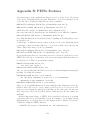
Appendix B: PETSc Features . . . . . . . . . . . . . . . . . . . . . . . . . . . . . . . . . . . . 118
Vita . . . . . . . . . . . . . . . . . . . . . . . . . . . . . . . . . . . . . . . . . . . . . . . . . . . . . . . . . . . . . 120
iv
List of Figures
1.1
Curve propagation with speed F in normal direction . . . . . . . .
5
1.2
Curve propagating with F = 1 . . . . . . . . . . . . . . . . . . . . .
6
1.3
Weak solutions of |u0| = 1, u(−1) = u(1) = 0 . . . . . . . . . . . . .
8
1.4
Solution of Equation (1.4) for ε = 1/5, 1/10, 1/20, 1/40, 1/100 . . .
9
1.5
Upwind Discretization - 2D case
1.6
Discretization for the 1-D case . . . . . . . . . . . . . . . . . . . . . 22
1.7
Grid points for Rouy-Tourin algorithm . . . . . . . . . . . . . . . .
24
1.8
Rouy-Tourin Iterations . . . . . . . . . . . . . . . . . . . . . . . . .
26
1.9
Sweeping in 2 directions . . . . . . . . . . . . . . . . . . . . . . . .
28
2.1
Dijkstra algorithm . . . . . . . . . . . . . . . . . . . . . . . . . . .
30
2.2
Far away, narrow band and accepted nodes . . . . . . . . . . . . . . 32
2.3
Update procedure for Fast Marching Method . . . . . . . . . . . . .
34
2.4
Matrix of neighboring nodes of Xi,j . . . . . . . . . . . . . . . . . .
41
2.5
Node Xi,j has only one accepted neighbor
. . . . . . . . . . . . . .
43
2.6
Node Xi,j has the neighbors Xi,j−1 and Xi+1,j accepted . . . . . . .
44
2.7
Node Xi,j has the neighbors Xi,j−1 and Xi,j+1 accepted . . . . . . .
47
3.1
Domain decomposition in sub-domains . . . . . . . . . . . . . . . . 50
3.2
Ghost points for a particular process . . . . . . . . . . . . . . . . .
51
3.3
Neighbors of Xi,j . . . . . . . . . . . . . . . . . . . . . . . . . . . .
53
3.4
Ghost points update . . . . . . . . . . . . . . . . . . . . . . . . . .
56
3.5
Ghost-zone influence on sub-domains . . . . . . . . . . . . . . . . .
58
3.6
Node Z is in the same sub-domain as Xi,j . . . . . . . . . . . . . .
61
3.7
Node Z is a ghost-node of Xi,j . . . . . . . . . . . . . . . . . . . . .
61
3.8
Node Z is in the same sub-domain as Xi,j . . . . . . . . . . . . . .
62
v
. . . . . . . . . . . . . . . . . . .
20
3.9
Node Z is a ghost-node of Xi,j . . . . . . . . . . . . . . . . . . . . .
63
4.1
Double-chained list structure . . . . . . . . . . . . . . . . . . . . . .
66
4.2
Deletion from the double-chained list . . . . . . . . . . . . . . . . .
69
4.3
Insertion after the current node in a double-chained list . . . . . . .
70
4.4
Insertion before the current node in a double-chained list . . . . . .
71
4.5
Sort algorithm . . . . . . . . . . . . . . . . . . . . . . . . . . . . . .
73
4.6
Sequential Fast Marching Algorithm Complexity . . . . . . . . . . .
75
4.7
L∞ error . . . . . . . . . . . . . . . . . . . . . . . . . . . . . . . . .
76
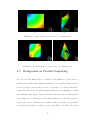
4.8
Solution’s shape for one processor - one starting node . . . . . . . .
77
4.9
Solution’s shape for one processor - two starting nodes . . . . . . .
77
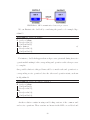
4.10 Shared memory architecture . . . . . . . . . . . . . . . . . . . . . .
79
4.11 Distributed memory architecture . . . . . . . . . . . . . . . . . . .
79
4.12 Hybrid shared-distributed memory architecture . . . . . . . . . . .
79
4.13 MPI communication between 2 processors . . . . . . . . . . . . . .
82
4.14 Global and Local Vectors . . . . . . . . . . . . . . . . . . . . . . . .
84
4.15 Natural and PETSC ordering for a Distributed Array . . . . . . . .
85
4.16 Domain structure with the points and ghost-points limits . . . . . .
87
4.17 Possible situation in ordered overlap strategy . . . . . . . . . . . . .
89
4.18 Back-propagation of the error . . . . . . . . . . . . . . . . . . . . . 95
4.19 Solution’s shape for multiple processors case . . . . . . . . . . . . .
95
4.20 Test cases . . . . . . . . . . . . . . . . . . . . . . . . . . . . . . . .
98
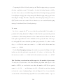
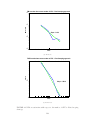
4.21 Time complexity for 50 CPU’s - Ordered Overlap Strategy . . . . . 101
4.22 Time Complexity for 50 CPU’s - Fast Sweeping Strategy . . . . . . 102
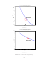
4.23 Time Complexity for both strategies . . . . . . . . . . . . . . . . . 104
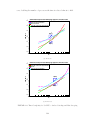
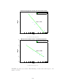
4.24 L∞ Error - Ordered Overlap Strategy . . . . . . . . . . . . . . . . . 106
4.25 L∞ Error- Fast Sweeping Strategy . . . . . . . . . . . . . . . . . . . 107
vi
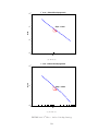
4.26 FM execution time - Ordered Overlap Strategy . . . . . . . . . . . 108
4.27 FM execution time - Fast Sweeping Strategy . . . . . . . . . . . . . 109
4.28 Best case scenario: Fast Marching execution time . . . . . . . . . . 110
4.29 Modules Hierachy . . . . . . . . . . . . . . . . . . . . . . . . . . . . 113
vii
List of Algorithms
1
The Rouy-Tourin algorithm . . . . . . . . . . . . . . . . . . . . . .
24
2
Fast Sweeping Algorithm . . . . . . . . . . . . . . . . . . . . . . . .
29
3
Fast Marching algorithm . . . . . . . . . . . . . . . . . . . . . . . .
33
4
Parallel Fast Marching algorithm . . . . . . . . . . . . . . . . . . .
55
5
Ghost-zones Synchronization procedure . . . . . . . . . . . . . . . .
55
6
Solution of the quadratic equation . . . . . . . . . . . . . . . . . . .
67
7
Solution of the local Eikonal equation at Xi,j . . . . . . . . . . . . .
67
8
Flag update . . . . . . . . . . . . . . . . . . . . . . . . . . . . . . .
68
9
Delete current node from the list . . . . . . . . . . . . . . . . . . .
69
10
Insert node Xi,j after current node . . . . . . . . . . . . . . . . . .
70
11
Insert node Xi,j before current node . . . . . . . . . . . . . . . . . .
71
12
UpdateList . . . . . . . . . . . . . . . . . . . . . . . . . . . . . . .
72
13
Basic MPI example . . . . . . . . . . . . . . . . . . . . . . . . . . .
81
14
MPI functions . . . . . . . . . . . . . . . . . . . . . . . . . . . . . .
81
15
Deadlock example . . . . . . . . . . . . . . . . . . . . . . . . . . . .
82
16
Deadlock solution - version 1 . . . . . . . . . . . . . . . . . . . . . .
82
17
Deadlock solution - version 2 . . . . . . . . . . . . . . . . . . . . . .
83
18
Ordered Overlap Algorithm . . . . . . . . . . . . . . . . . . . . . .
90
19
Boundary recomputation based on ghost-points . . . . . . . . . . .
91
20
Fast Sweeping Boundary Update . . . . . . . . . . . . . . . . . . .
92
21
Flag update on the sub-domains . . . . . . . . . . . . . . . . . . . .
93
22
Main Function . . . . . . . . . . . . . . . . . . . . . . . . . . . . . . 114
23
Structure Module Header . . . . . . . . . . . . . . . . . . . . . . . . 114
24
List module header . . . . . . . . . . . . . . . . . . . . . . . . . . . 115
viii
25
Flag Module Header . . . . . . . . . . . . . . . . . . . . . . . . . . 115
26
Algorithms Module Header . . . . . . . . . . . . . . . . . . . . . . . 116
27
Display Module Header . . . . . . . . . . . . . . . . . . . . . . . . . 117
28
String Conversion Module Header . . . . . . . . . . . . . . . . . . . 117
ix
Abstract
Fast Marching represents a very efficient technique for solving front propagation
problems, which can be formulated as partial differential equations with Dirichlet
boundary conditions, called Eikonal equation:


 F (x)|∇T (x)| = 1,


T (x)
= 0,
x∈Ω
x ∈ Γ,
where Ω is a domain in Rn , Γ is the initial position of a curve evolving with normal
velocity F > 0. Fast Marching Methods are a necessary step in Level Set Methods,
which are widely used today in scientific computing. The classical Fast Marching
Methods, based on finite differences, are typically sequential. Parallelizing Fast
Marching Methods is a step forward for employing the Level Set Methods on
supercomputers.
The efficiency of the parallel Fast Marching implementation depends on the required amount of communication between sub-domains and on algorithm ability
to preserve the upwind structure of the numerical scheme during execution. To address these problems, I develop several parallel strategies which allow fast convergence. The strengths of these approaches are illustrated on a series of benchmarks
which include the study of the convergence, the error estimates, and the proof of
the monotonicity and stability of the algorithms.
x
Introduction
Scientific computing allows scientists and engineers to gain understanding of real
life problems in diverse areas, such as cosmology, climate control, computational
fluid dynamics, health-care, design and manufacturing. The scientists and engineers develop computer programs that model the behavior of the studied system
or phenomenon. Running these programs with multiple and various sets of input
parameters helps them better comprehend past behavioral patterns and possibly
predict future actions. Typically, these models require massive amounts of calculations and, therefore, executed on supercomputers or distributed computing
platforms.
Nowadays, parallel computing is considered a standard tool for scientific computing. It is formally viewed as the simultaneous use of multiple processors to execute
a program. Parallel programming is more intricate than its sequential counterpart
and demands extra care. For instance, concurrency between tasks introduces several new classes of potential software bugs and requires revisiting many classical
algorithms. Communication and synchronization between processors is typically
one of the greatest barriers to getting good performances. All of these are aspects
that I have encountered while preparing my thesis.
In order to set this work into perspective, let me describe first the front propagation problem that I want to solve employing parallel computing. It is known
that interfaces propagation occur in a lot of settings, including ocean waves, material boundaries, optimal path planning, construction of geodesic path on surfaces,
iso-intensity contours in images, computer vision and many more. I consider the
case of a curve propagating in a domain with a normal velocity F > 0, the tangent
direction of the movement being ignored. I want to track the motion of this in-
1
terface as it evolves. To describe interface motion, I formulate the boundary value
problem and the partial differential equation with initial value known as Eikonal
equation:


 F (x)|∇T (x)| = 1,


T (x)
= 0,
x∈Ω
x ∈ Γ,
where Ω is a domain in Rn , Γ is the initial position of a curve evolving with normal
velocity F, ∇ denotes the gradient, and | · | is the Euclidean norm. The solution T
of the Eikonal equation can be view as: the time of first arrival of the curve Γ, or
as the distance function to curve Γ, if F = 1. All the mathematical details on how
to find the solution to Eikonal equation are presented in Chapter 1.
The primary goal of my thesis is to solve the Eikonal equation employing parallelized computational methods and algorithms. To solve this equation, I use the
Fast Marching Method, a computational technique for tracking moving interfaces
and modeling the evolution of boundaries. Fast Marching Methods are typically
sequential, and hence not straight forward to parallelize [18, 23]. The Fast Marching algorithm is a necessary step in Level Set Methods, which, in today’s scientific
computing world, are widely used for simulating front motion related processes.
Therefore, since they have a great impact on many applications, it is imperative
to parallelize Fast Marching Methods to try to improve even more execution time
and solution accuracy.
The idea of the parallel Fast Marching algorithm is to perform Fast Marching on sub-domains, update the boundary values at the interfaces and restart the
algorithm until convergence is achieved. To update the boundary values at the
interfaces we need to preserve the upwind structure of the numerical scheme and
to synchronize the ghost-zones at each iteration. Therefore, the efficiency of the
parallel Fast Marching implementation depends on the required amount of com-
2
munication between sub-domains and on algorithm ability to preserve the upwind
structure of the numerical scheme during execution. To address these problems, I
develop several strategies, among which the following are the most viable:
1. Ordered Overlap strategy: group the overlapping nodes of each sub-domain
in a sorted list and use this list to recompute the boundary values;
2. Fast Sweeping strategy: perform a Fast Sweeping [28] at the interfaces and
update the overlapping regions of the sub-domains.
The advantage of these strategies is to not keep a distributed list for the narrow
band, which would require much more communication time.
The thesis is organized as follows.
In Chapter 1, I present the theoretical background necessary to deal with the
problem of moving interfaces. I begin by introducing the Hamilton-Jacobi equations
and viscosity solution, emphasizing the Eikonal equation and its application. In
the second part of this chapter, I explain the numerical approximation scheme and
the numerical methods used to solve the Eikonal equation over the past years.
Specifically, I talk about the main features of the Rouy-Tourin algorithm [21] and
the Fast Sweeping algorithm [28].
Chapter 2 is devoted to the sequential Fast Marching Methods, which “are the
optimal way to solve Hamilton-Jacobi equations” [23]. I begin by explaining the
idea of classifying the nodes as accepted, narrow band and far away. I follow with
the description of the algorithm, pointing out how the upwind nature of the numerical scheme is preserved. I end up presenting how the numerical solution built
by the Fast Marching Methods converges to the viscosity solution of the Eikonal
equation. To prove this, I first show how the solution of the discrete Eikonal equation converges to the viscosity solution [3]. Secondly, I show that the sequence
3
built by the Fast Marching Methods converges to the solution of discrete Eikonal
equation.
Chapter 3 deals with the parallel Fast Marching Methods. First of all, I focus
on formulating the problem in terms of parallel programing. I define the necessary
notions, such as sub-domains, neighbors, ghost-nodes, ghost-zones. After that, I
present the convergence results for the parallel Fast Marching algorithm.
Chapter 4 focuses on the aspect of implementation and on numerical experiments. The chapter starts with a brief presentation of the sequential implementation and elaborates the main problems through numerical experiments. Then,
it gives a short background on parallel computing before focusing on the actual
parallel implementation of the algorithm. I bring to one’s attention parallel programming concepts, such as parallel architectures, programming models, and the
issues that differentiate it from sequential programming. I also focus on the obstacles encountered during parallel implementation and how to get over them. I
illustrate the strengths of the parallel approach with a series of benchmarks, which
include the study of convergence, error estimates. In addition, I show the algorithm
is monotone and stable.
4
Chapter 1
Background
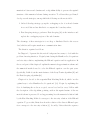
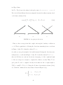
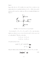
Let us consider a boundary (a closed curve in two dimensions or a surface in three
dimensions), separating two regions. Let this curve or surface evolve with a known
normal velocity F as shown in Figure 1.1. The function F may depend on factors
such as curvature, normal direction, shape and position of the front, or shape
independent properties [23].
Assume that the curve moves outwards from the domain (i.e. F > 0) and the
tangential direction of the motions are ignored. In all that follow, we will consider
that F depends on the position of the front and not on curvature.
F
:
(x, y)
FIGURE 1.1. Curve propagation with speed F in normal direction
In order to characterize the position of the expanding front, we can compute
its first arrival time T as it crosses each point (x,y) in the domain. Therefore, we
define T (x, y) = inf Γt , (x, y) ∈ Γt .
t>0
5
Formally, in one dimension we have distance = rate × time, so we can write the
equation for the arrival function T :
1=F
dT
.
dx
In higher dimensions, the time T of first arrival is the solution of a boundary
value problem, known as the Eikonal equation:


 F (x)|∇T (x)| = 1,


T (x)
= 0,
x∈Ω
(1.1)
x ∈ Γ,
where Ω is a domain in Rn , Γ is the initial position of a curve evolving with normal
velocity F, ∇ denotes the gradient, and | · | is the Euclidean norm.
We want to show how the time of first arrival is different from the curve evolution.
For illustration purposes consider the propagation of a curve, with normal velocity
F = 1, as presented in Figure 1.2.
(a) Swallowtail
(b) Physically Correct Evolution
FIGURE 1.2. Curve propagating with F = 1
In Figure 1.2(a), the curve passes through itself developing the so-called swallowtail. Analyzing the swallowtail from the geometric point at view, at a time t,
we have a multivalued solution. Since “the solution should consist of only the set
of all points located a distance t from the initial curve” [22], we need to remove
the “tail” from “swallowtail”. In [23], Sethian described this situation as: “if the
6
front is viewed as a burning flame, then once a particle burnt it stayed burnt”.
Therefore, from the family of solutions, we pick the physically reasonable solution,
with the shape presented in Figure 1.2(b).
Equation (1.1) is a particular form of first-order Hamilton-Jacobi equation.
The Dirichlet problem for a static Hamilton-Jacobi equation can be written in
the form:


 H(x, Du) = 0 on Rn × (0, ∞)

 u=φ
(1.2)
n
on R × {t = 0} ,
where the Hamiltonian H = H(x, Du) is a continuous real valued function on
Rn × Rn ([8], pg. 539), and φ : Rn → R is a given initial function.
In general, this equation does not have classical solutions, i.e. solutions which are
C 1 . The problem does have generalized solutions, which are continuous and satisfy
the partial differential equation almost everywhere. Using the notion of viscosity
solution, introduced by Crandall and Lions [4, 5] for first-order problems, one can
choose the correct “physical” solution from the multitude of solutions.
1.1
1.1.1
Viscosity Solutions
Motivation
Let us consider the unidimensional Eikonal equation with homogeneous Dirichlet
boundary condition:


 |u0(x)| = 1 in (−1, 1)
(1.3)

 u(x) = 0, x = ±1.
The general solution of the differential equation is u = ±x + c. We cannot choose
a sign for x and a constant of integration to satisfy both boundary conditions, but
there are weak solutions that satisfy the differential equation almost everywhere.
7
The function:
u(x) = 1 − |x|
satisfies the boundary conditions and satisfies the differential equation everywhere
except x = 0. This solution gives the distance to the boundary of the domain, but
is not unique. As shown in Figure 1.3, there exists infinitely many weak solution:
continuous function with slope ±1, satisfying almost everywhere the boundary
conditions.
(a)
(b)
(c)
(d)
FIGURE 1.3. Weak solutions of |u0 | = 1, u(−1) = u(1) = 0
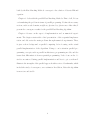
By adding a small viscosity term to Equation (1.3), one can obtain a secondorder equation for uε (x):


 −εu00 + |u0 | = 1 in (−1, 1)
ε
ε

 uε (−1) = uε (1) = 0, ε ≥ 0.
It is well known that equation (1.4) has a unique solution of the form:
uε (x) = 1 − |x| + εe−1/ε (1 − e(1−|x|)/ε ).
8
(1.4)
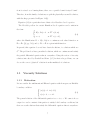
In Figure 1.4 we graph the solution of equation (1.4) for ε = 1/5, 1/10, 1/20, 1/40,
1/100. For small ε, the viscosity term smooths out part of the solution uε (x). In
fact, it will smooth out the corners to make the solution C 2 . In this example we
choose ε > 0 to smooth the solution at its relative maximum. By choosing ε < 0,
one would obtain an approximation of u(x) = |x| − 1, which smooths the solution
at relative minimum point. As ε → 0, uε converges to the viscosity solution of
(1.3), which is introduced in more details in the following section.
1
ε = 1/5
ε = 1/10
ε = 1/20
ε = 1/40
ε = 1/100
← ε = 1/100
0.8
← ε = 1/5
0.6
0.4
0.2
0
−1
−0.5
0
0.5
1
FIGURE 1.4. Solution of Equation (1.4) for ε = 1/5, 1/10, 1/20, 1/40, 1/100
1.1.2
The General Case
Let Ω be an open bounded domain in Rn , Γ ⊂ ∂Ω and consider the general static
Hamilton-Jacobi equation:


 H(x, Du) = 0 on Ω

 u=φ
(1.5)
on Γ ⊆ ∂Ω,
where H is convex, u and φ are continuous.
As Crandall, Evans and Lions pointed out in [4] and [5], problem (1.5) does not
have, in general, a C 1 solution. It admits generalized (weak) solutions. Hence, we
9
can approximate the problem by adding a viscosity term to (1.5):


 H(x, Duε ) − ε∆uε = 0 on Ω

 uε = φ
(1.6)
on Γ ⊆ ∂Ω,
for ε > 0. Problem (1.6) admits a smooth solution uε [4, 5, 8].
We want to prove that as ε → 0, the solution uε (x) of (1.6) converges locally
uniformly to a weak solution u of (1.5). In order to do that, we follow Evans’s
arguments, presented in [8]. This method is known as the method of vanishing
viscosity. When ε → 0, we can find a family of functions {uε }ε>0 , which is uniformly
bounded and equicontinuous on a compact subset of Ω ⊂ Rn . Applying the ArzelaAscoli compactness criterion, there exists a subsequence uεj ⊆ uε such that
uεj → u locally uniformly in Ω ⊂ Rn .
(1.7)
At this point, we can expect u to be some kind of solution of our initial-value
problem (1.5), but we only know that u is continuous and we do not have any
information on the derivatives of u. As ε → 0, we do not have a uniform bound on
Duε , which would allow us to show that Duε → Du in some sense. To prove that,
we introduce a smooth test function v ∈ C ∞ (Ω), v|Γ = 0, and suppose that
u − v has a strict local maximum at x = x0 ∈ Ω.
(1.8)
This means u(x0 ) − v(x0 ) > u(x) − v(x) in some neighborhood of x0 , with x 6= x0 .
Recalling (1.7) we claim that for each εj > 0 sufficiently small enough, there exists
a point xεj such that
uεj − v has a local maximum at xεj , and xεj → x0 as j → ∞.
(1.9)
To confirm this, note that for each sufficient small r > 0, equation (1.8) implies
max(u − v) < (u − v)(x0 ), where B(x0 , r) is the closed ball in Ω ⊂ Rn with center
∂B
10
at x0 and radius r. Applying Arzela-Ascoli compactness criterion, we claim that
for εj small enough, uεj → u uniformly on B and max(uεj − v) < (uεj − v)(x0 ).
∂B
Consequently uε − v attains a local maximum at some point in the interior of B.
Considering now a radii sequence rj such that rj → 0, we obtain (1.9).
Using the second derivative test and relation (1.9) we can relate the derivatives of
uεj and v:
Duεj (xεj )
= Dv(xεj )
(1.10)
−∆uεj (xεj ) ≥ −∆v(xεj )
We show that H(x0, Dv(x0)) ≤ 0:
H(xεj , Dv(xεj )) = H(xεj , Duεj (xεj )) (using 1.10)
= εj ∆uεj (xεj ) (using 1.6)
≤ εj ∆v(xεj ) (using 1.10).
Since v is smooth, H is continuous, xεj → x0 as j → ∞ and letting εj → 0, the
previous inequality becomes
H(x0 , Dv(x0 )) ≤ 0.
(1.11)
Similarly, we deduce the inverse inequality:
H(x0 , Dv(x0 )) ≥ 0,
(1.12)
u − v has a local minimum at x0 .
(1.13)
provided that
Equations (1.8), (1.11), (1.13) and (1.12) define the concept of weak solution of
(1.5) as:
Definition 1.1 (version I). A bounded, uniformly continuous function u is a viscosity solution of the initial-value problem (1.5) for the Hamilton-Jacobi equation
11
provided that the function satisfies the boundary condition: u = φ on ∂Ω and for
all v ∈ C ∞ (Ω):
if u − v has a local maximum at x0 , then H(x0 , Dv(x0 )) ≤ 0,
(1.14)
(u is called a viscosity sub-solution)
and
if u − v has a local minimum at x0 , then H(x0 , Dv(x0 )) ≥ 0
(1.15)
(u is called a viscosity supra-solution).
Remark 1.2. In the light of Definition 1.1, u defined in (1.7) and solution of (1.6)
converges to the viscosity solution of (1.5).
To verify that a given function u is a viscosity solution of the Hamilton-Jacobi
equation H(x, Du) = 0, equations (1.14) and (1.15) must hold for all smooth
functions v. Evans noted in [8] that if we used the vanishing viscosity method to
construct u, then it would indeed be a viscosity solution.
Viscosity solutions can be seen as the limit function u = lim uε , where uε ∈
ε→0
2
C (Ω) is the classical solution of the perturbed problem (1.6), if uε exists and converges locally uniformly to some continuous function u.
If φ is bounded and uniformly continuous, then u is the unique viscosity solution
of (1.5). One can extend the notion of viscosity solution of (1.5) for φ discontinuous, using the lower semi-continuous (l.s.c) and the upper semi-continuous (u.s.c)
envelopes of the solution [2].
Definition 1.3. For any x ∈ Ω, define the upper semi-continuous envelope of u
as:
ū(x) = lim sup u(y),
y→x
and the lower semi-continuous envelope of u as:
u(x) = lim inf u(y).
y→x
12
Therefore, we can rewrite the definition of the viscosity solution:
Definition 1.4 (version II). A locally bounded function u is a viscosity sub-solution
of the Hamilton Jacobi equation (1.5) if
∀ v ∈ C 1 (Rn ), at each maximum point x0 of ū − v, we have:
max {H(x0 , Dv(x0)), ū − φ} ≤ 0
and a viscosity super-solution of the Hamilton Jacobi equation (1.5) if
∀ v ∈ C 1 (Rn ), at each minimum point x0 of u − v, we have:
max {H(x0 , Dv(x0 )), u − φ} ≥ 0.
Remark 1.5. Then u is a viscosity solution of (1.5) if u is both a sub-solution
and super-solution.
Remark 1.6. Definition (1.4) is an extension of Crandall-Lions or Ishii definition of viscosity solution for continuous Hamiltonians (see [2] pg. 558-577, [5, 13]).
Definition (1.1) is a particular case of Definition (1.4) for continuous Hamiltonians.
Viscosity solutions have the following properties: consistency, existence, uniqueness and stability. One can show that the viscosity solution satisfies the partial
differential equation (1.5) whenever it is differentiable, that it exists, and furthermore it is unique and stable.
Theorem 1.7 (Consistency of a viscosity solution). Let u be a viscosity solution
of problem(1.5) and suppose u is differentiable at some point x0 ∈ Ω ⊂ Rn . Then
H(x0 , Du(x0 )) = 0.
The proof of this theorem can be found in [8], section 10.1.2, page 545.
Proposition 1.8. If u ∈ C 1 (Ω) solves (1.5) and if u is bounded and uniformly
continuous, then u is a viscosity solution.
13
Proof. If v is smooth and u−v has a local maximum at x0 , then Du(x0 ) = Dv(x0 ).
This implies that H(x0 , Dv(x0 )) = H(x0 , Du(x0 )) = 0, since u solves (1.5). Similar
equality holds for u − v having a local minimum at x0 .
Theorem 1.9 (Existence and uniqueness). Let Ω be a bounded open subset of Rn ,
H convex on Ω, H ≥ 0; also let F : Ω → R such that F > 0 is continuous on Ω̄.
Then there exists a unique viscosity solution u of the problem:


 F (x)H(x, ∇u) = 0, x ∈ Ω

 u(x) = 0,
(1.16)
x ∈ Γ ⊆ ∂Ω,
Crandall and Lions proved this theorem in [5], pages 24-25, and pointed out
assumptions that can cause the uniqueness of the viscosity solution to fail.
Remark 1.10. If the function F vanishes at at least a single point in Ω, then the
uniqueness result does not hold. It can be proved that in this case many viscosity
solutions or even classical solutions may exist.
Theorem 1.11. Assume u1 , u2 ∈ C(Ω̄), where Ω ⊂ Rn is open and bounded, are a
viscosity sub-solution and a super-solution of H(x, ∇u(x)) = 0, x ∈ Ω and u1 ≤ u2
on ∂Ω. Assume also that H satisfies the conditions of Lipschitz continuity:
|H(x, p) − H(y, q)| ≤ C(|p − q|)
and
|H(x, p) − H(y, q)| ≤ C(|x − y|(1 + |p|))
(1.17)
for x, y ∈ Ω, p, q ∈ Rn , and some constant C ≥ 0.
Then u1 ≤ u2 ∈ Ω̄.
Remark 1.12. Assuming that the Hamiltonian H satisfies the conditions of Lipschitz continuity, Evans proves that there exists at most one viscosity solution of
(1.5) ([8], Theorem 1, pg. 547).
14
We need to assume that H is convex with respect to the variable p, in order
to apply this theorem to more general cases. This assumption is the key point in
many theoretical results.
Proposition 1.13 ( Stability Property). Let {un }n∈N ∈ C 0 (Ω) be a sequence of
functions such that un is the viscosity solution of the problem
Hn (x, ∇un ) = 0, x ∈ Ω, n ∈ N.
Assume that un converges locally uniformly to u and Hn converges locally uniformly
to H. Then u is the viscosity solution of
H(x, ∇u) = 0, x ∈ Ω.
Theorem 1.14. Let Ω be a bounded and open subset of Rn . Assume that u1 , u2 ∈
C(Ω̄) are the viscosity sub-solution and super-solution of equation (1.5), with u1 <
u2 on ∂Ω. Assume also that H = H(x, p) is convex with respect to the variable p
on Rn for each x ∈ Ω, and satisfies (1.17) and the following conditions:


 ∃ φ ∈ C(Ω̄) ∩ C 1 (Ω) such that φ ≤ u1 in Ω̄ and

 sup H(x, ∇φ(x)) < 0, for all Ω0 ⊂ Ω.
(1.18)
x∈Ω0
Then u1 ≤ u2 in Ω.
This theorem can be applied to the Eikonal equation whenever F (x) is Lipschitz
in Ω and it is strictly positive [6]. Conditions (1.18) are satisfied by taking
φ(x) = min u1 .
x∈Ω̄
1.1.3
Application to the Eikonal Equation
Proposition 1.15. Let Ω be bounded open subset of Rn . Set u(x) = distance(x, ∂Ω),
x ∈ Ω. Then u is Lipschitz continuous and is a solution of the Eikonal equation:
|Du| = 1 in Ω.
15
This means that for each v ∈ C ∞ (Ω), if u − v has a maximum (minimum) at a
point x0 ∈ Ω, then |Dv(x0 )| ≤ 1 (|Dv(x0)| ≥ 1).
In the initial model problem (1.5), we can obtain the Eikonal equation, by considering the Hamiltonian H(x, Du) = F |∇u| − 1.
For a general set Ω, we have the following corollary.
Corollary 1.16. If F (x) > 0 for all x ∈ Ω ⊂ Rn , then the equation


 F (x)|∇T (x)| = 1, x ∈ Ω ⊂ Rn

 T (x) = 0,
(1.19)
x ∈ Γ,
admits a unique viscosity solution T .
Remark 1.17. In [9] it is proved that if F is Lipschitz in Rn ∩ L∞ (Rn ), then the
unique viscosity solution T is locally Lipschitz in Ω.
For the front propagation problems, we want to have an Eulerian formulation
for the motion of the initial curve Γt=0 ⊂ Ω, under the influence of normal velocity
F > 0. We interpret the solution T (x, y) of the Eikonal equation as the time needed
by the curve Γt to evolve and reach the point (x, y) for the first time. We consider
the t-level set of T (x, y) as the zero-level set of the viscosity solution of the Eikonal
equation at time t: Γ0 (t) = {(x, y)|T (x, y) = t}.
Remark 1.18. When F = 1, T is also interpreted as the distance to Γ0 .
The gradient flow of T gives the trajectories of each point.
Property 1.19 (Optimality Property). Let curve Γ propagate in the domain Ω
with normal velocity F > 0 and T (x, y) be the viscosity solution of (1.19). Let
Γ0 (t) = {(x, y)|T (x, y) = t} be the zero-level set of the solution T . The trajectory
of a point (x, y) of the front coincides with the trajectory starting at (x0 , y0 ) ∈ Γ0
and reaching (x, y) in time t.
16
The way of interpreting T , in the light of the last property, is very important
for the construction of all numerical schemes. Since T is the viscosity solution,
the trajectory of a point (x, y) is the “physically” correct trajectory from all the
possible ones starting from (x, y).
1.2
Numerical Approximations
In this section we present a numerical scheme to compute the viscosity solution of
the Eikonal equation (1.1), under the assumption that F (x) > 0 on Ω.
It is shown in [26] that the first-arrival travel-time field is a viscosity solution of the
Eikonal equation. Numerical methods utilizing upwind finite differences schemes
manage to produce viscosity solutions of the Eikonal equation. If we consider the
numerical methods to approximate the partial differential equation, then we distinguish the following methods: the algorithm introduced by Rouy and Tourin [21],
the Fast Sweeping algorithm [28], the Fast Marching Methods proposed by Osher
and Sethian [18]. They all compute an approximation of the same solution.
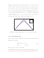
1.2.1
Motivation
Let Ω = (0, 1) and consider the one-dimensional Eikonal equation given by:
p
u2x = F (x), u(−1) = u(1) = 0.
Given the speed function F (x) > 0, we want to construct u(x) away from the
boundary and we observe that the solution is not unique (for instance, if v(x) solves
the problem, then so does −v(x)). We will deal only with nonnegative solutions of
the function u.
Consider the following ordinary differential equations and try to solve each problem
17
separately:





if x ≥ 0,

du  F (x),


=
dx 
 −F (x), if x ≤ 0,




 u(−1) = u(1) = 0.
In order to do the numerical approximation, we partition the x-axis into a collection
of grid points xi = i∆x and define ui = u(i∆x) and Fi = F (i∆x), where ∆x is the
discretization step, and i = −n, · · · , n. Using a Taylor expansion and neglecting
the remainder we obtain the discrete system:



un = 0,






 ui+1 − ui = Fi , i > 0,
∆x
u
−
ui−1

i

= −Fi , i ≤ 0,



∆x



 u−n = 0.
Notice that
un−1 can be computed exactly from un
un−2 can be computed exactly from un−1
···
u1 can be computed exactly from u2
u0 can be computed exactly from u1
···
u−n+1 can be computed exactly from u−n
u−n+2 can be computed exactly from u−n+1
···
u−1 can be computed exactly from u−2
u0 can be computed exactly from u−1 .
This is an upwind scheme: we compute derivatives using points “upwind” or toward the boundary condition (i.e., each ordinary differential equation is solved
18
away from the boundary condition).
Modeling numerically the Eikonal equation, we consider that the information is
propagating like waves, with certain speeds, along the gradient directions. The
upwind discretization methods compute the values of the variables using the
direction(s) from which the information should be coming. More precisely, the
discretization of the partial differential equations uses a finite differences stencil,
biased on the direction determined by the sign of the gradient [16]. The upwind
scheme uses backward differences scheme if the velocity is in the positive x direction, and forward differences scheme for negative velocities. Thus, in a onedimensional domain, for any point i we have only two direction: left (i − 1) and
right (i + 1). If the velocity is positive, the left side of the axis is called upwind
side and the right side is called downwind side, and vice versa for negative velocities.
Let uni be the computed solution at the point i at iteration n. We have the following
schemes:
1. Forward scheme: un+1
= uni − ∆xDi+x uni ,
i
2. Backward scheme: un+1
= uni − ∆xDi−x uni .
i
Similarly to the one dimensional case, using forward, backward or centered Taylor
series expansions in x and y for the value u around the point (x, y), with (xi , yj ) =
(i∆x, j∆y) and uij = u(xi , yj ) we can define four differentiation operators for the
two-dimensional case:
ui,j − ui−1,j
∆x
ui,j − ui,j−1
−y
Di,j u(xi , yj ) =
∆y
−x
u(xi , yj ) =
Di,j
ui+1,j − ui,j
∆x
ui,j+1 − ui,j
+y
Di,j u(xi , yj ) =
∆y
+x
Di,j
u(xi , yj ) =
where
19
(1.20)
• D +x computes the new value at (i, j) using information at i and i + 1; thus
information for the solution propagates from right to left.
• D −x computes the new value at (i, j) using information at i and i − 1; thus
information for the solution propagates from left to right.
• D +y computes the new value at (i, j) using information at j and j + 1; thus
information for the solution propagates from top to bottom.
• D −y computes the new value at (i, j) using information at j and j − 1; thus
information for the solution propagates from bottom to top.
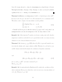
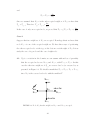
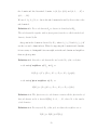
For two-dimensional domains, the upwind method uses the gradient direction in
order to select which differentiation operator to use. In Figure 1.5 we illustrate
only two possible situations, all the other cases being similar up to a rotation in
the system of coordinates. In case 1.5(a) we use the backward differences scheme
in x and y and define the third quadrant as the upwind side. In case 1.5(b) we
use backward differences in x and forward differences in y and the upwind side is
quadrant two.
i,j+1
i,j+1
Du
i-1,j
i-1,j
i,j
i,j
i+1,j
i,j-1
Du
i+1,j
i,j-1
(a)
(b)
FIGURE 1.5. Upwind Discretization - 2D case
20
1.2.2
Approximations of the Eikonal Equation
Crandall and Lions [5] proved that consistent, monotone schemes converge to the
correct viscosity solution. Starting from equation (1.1), in order to construct a
numerical scheme which guarantees a correct upwind direction and a correct approximation of the viscosity solution, it is necessary to have a good approximation
of the derivative. Extending the ideas of upwind approximations for the gradient
to multiple dimensions, we have the following schemes:
• Godunov’s scheme [16]
2
[max Dij−x T, −Dij+x T, 0
+
2
max Dij−y T, −Dij+y T, 0 ]1/2 =
(1.21)
1
,
Fij
• Osher and Sethian’s scheme [18]
[max(Dij−x T, 0)2 + min(Dij+x T, 0)2
max(Dij−y T, 0)2
+
+ min(Dij+y T, 0)2 ]1/2 =
1
,
Fij
where the forward and backward operators Dij−x , Dij+x are those defined earlier
in equation (1.20) for the x and y directions.
Remark 1.20. Rewriting Godunov’s scheme, we obtain the so called Rouy-Tourin’s
scheme [21]:
[max[max Dij−x T, 0 , −min Dij+x T, 0 ]2
+
max[max Dij−y T, 0 , −min Dij+y T, 0 ]2 ]1/2 =
1
.
Fij
(1.22)
Recall the boundary value problem F |∇T | = 1 can be written in the form of
general Hamilton Jacobi equation:
H(x, y, D xT, Dy T ) = 0,
21
where the Hamiltonian is given by:
H(x, y, D xT, Dy T ) = F
p
(D x T )2 + (D y T )2 − 1.
(1.23)
To solve numerically the Eikonal equation, we need a correct approximation
of the viscosity solution [18, 22, 24]. A smart way to do this is to consider only
numerical schemes which satisfy the upwind condition. These schemes ensure that,
out of all possible T such that F |∇T | = 1 almost everywhere, only the correct
“physical” solution from the family of solutions of (1.22) is picked. Since T solves
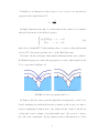
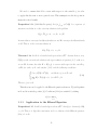
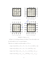
equation (1.22), T cannot be locally convex. In Figure 1.6 we consider a stencil
with ∆x = 1 and F (x) = 1, 1 < i < n and show how it selects only concave
solutions:
i-1
i
i+1
i-1
(a)
i
i+1
i-1
(b)
i-1
i
i
i+1
(c)
i+1
(d)
FIGURE 1.6. Discretization for the 1-D case
−x
+x
Case a : If Ti,j = Ti−1,j + 1 and Ti+1,j = Ti,j + 1, then Di,j
T = 1 and Di,j
T = 1.
Equation (1.22) becomes:
2
−x
+x
max max(Di,j
T, 0), − min(Di,j
T, 0) = [max(1, 0)]2 = 1.
22
−x
+x
Case b : If Ti−1,j = Ti,j + 1 and Ti,j = Ti+1,j + 1, then Di,j
T = −1 and Di,j
T = −1.
Equation (1.22) becomes:
2
−x
+x
max max(Di,j
T, 0), − min(Di,j
T, 0) = [max(0, 1)]2 = 1.
−x
+x
Case c : If Ti,j = Ti−1,j + 1 and Ti,j = Ti+1,j + 1, then Di,j
T = 1 and Di,j
T = −1.
Equation (1.22) becomes:
2
−x
+x
max max(Di,j
T, 0), − min(Di,j
T, 0) = [max(1, 1)]2 = 1.
−x
+x
Case d : If Ti−1,j = Ti,j + 1 and Ti+1,j = Ti,j + 1, then Di,j
T = −1 and Di,j
T = 1.
Equation (1.22) becomes:
2
−x
+x
max max(Di,j
T, 0), − min(Di,j
T, 0) = [max(0, 0)]2 = 0.
Thus, this case is not feasible and it is clear that the scheme selects only the
concave solution.
Remark 1.21. At this point we need to choose which discretization scheme to use
in the following steps of the numerical implementation. We settled for Rouy-Tourin
discretization scheme (1.22), since it is the easiest one to implement.
1.2.3
Numerical Methods
There have been lots of trials to solve the Eikonal equation directly: starting from
upwinding schemes [26], Jacobi-iterations [21], semi-Lagrangian schemes [11], fast
marching type methods [18, 24], fast sweeping methods [28] and many others methods. In the following subsections we briefly present the Rouy-Tourin and Fast
Sweeping algorithms.
1.2.3.1 Rouy-Tourin Algorithm
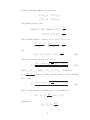
An iterative algorithm for computing the solution of Eikonal equation was introduced by Rouy and Tourin in [21]. The idea of this algorithm is to solve the
quadratic equation (1.22) at each point of the grid, and iterate until convergence.
23
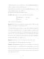
In Figure 1.7 we present the stencil structure for Rouy-Tourin algorithm and the
algorithm is presented in Algorithm 1.
Ti,j+1
Ti-1,j
R
Ti+1,j
Ti,j-1
FIGURE 1.7. Grid points for Rouy-Tourin algorithm
Algorithm 1 The Rouy-Tourin algorithm
Consider S > diam(Ω).
Initialization:
Ti,j = 0 on ∂Ω
Ti,j = S, otherwise
Iteration:
repeat
for i = 0 to n do
for j = 0 to n do
compute R solution of local Eikonal equation at Xi,j
end
end
T˜i,j = min(Ti,j , R)
T = T̃
until kT − T̃ k ≤ ε ;
For any node (i, j) in the domain we should solve the equation:
2
−x
+x
[ max max(Di,j
T, 0), − min(Di,j
T, 0)
+
2
−y
+y
max max(Di,j
T, 0), − min(Di,j
T, 0) ]1/2 =
1
,
Fi,j
(1.24)
in order to compute its Ti,j .
Let us consider the case presented in the previous section, in Figure 1.5(a), where
the third quadrant is the upwind side of our domain and show how the Rouy-Tourin
algorithm satisfies the upwind-ing. All the other possible situations can be reduced
24
to this case, based on rotation and symmetry of the domain. By evaluating:
Ti,j − Ti−1,j
≥0
∆x
Ti,j − Ti,j−1
=
≥0
∆y
Ti+1,j − Ti,j
≥0
∆x
Ti,j+1 − Ti,j
=
≥ 0,
∆y
−x
Di,j
Ti,j =
+x
Di,j
Ti,j =
−y
Di,j
Ti,j
+y
Di,j
Ti,j
and plugging them in equation (1.24), we obtain:
q
2
2
−y
−x
max Di,j
T, 0 + max Di,j
T, 0 =
q
1
−y 2
−x 2
Di,j
T + Di,j
T =
,
Fi,j
which is the quadratic equation that we need to solve:
s
2 2
1
Ti,j − Ti,j−1
Ti,j − Ti−1,j
.
+
=
∆x
∆y
Fi,j
During the algorithm execution, this computation is done many times for each
node in the domain, until convergence is achieved. Basically, the value at the grid
point Ti,j can be computed exactly using only T at its neighbors, i.e. Ti±1,j and
Ti,j±1. We consider T to be computed exactly, if and only if the new T is smaller
than the old one.
Remark 1.22. Since during the algorithm execution, at each iteration, we recompute T at every point of the domain, we have a lot of useless computations (T is
changing only at a few grid points). The algorithm is not taking this shortcut into
consideration.
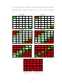
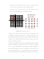
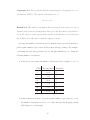
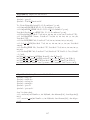
To illustrate the Rouy-Tourin algorithm, we consider a rectangular domain, with
the boundary condition imposed in two opposite corners. In the initialization step,
if Xi,j ∈ Γ (a point where we can approximate the initial curve), then T (Xi,j ) = 0,
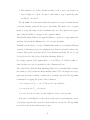
otherwise T (Xi,j ) = ∞. For exemplification purposes, Figure 1.8 shows the stages
of the algorithm for a particular case. At each iteration of the algorithm, we solve
the local Eikonal equation at all the points of the domain. Note how T changes
25
only at a few grid points. In Figure 1.8, these points are shown in green, while the
points with exactly computed T are represented by red cells, and the points where
Iteration 0
0

Iteration 1

0
0
1

Iteration 2
0
1
2

1
1.71

1.71
1

2
1
0
0
1
2
3

1
1
2
3

1.71 2.55

2.55

2.55 1.71

3
2
1
Iteration 4
0
1
2
3
4

1
0
Iteration 3

2
2

3
2
1
0
Iteration 5
1
2
3
4
1.71 2.55 3.44
2.55 3.25 3.44
3.44 3.25 2.55
3.44 2.55 1.71
4
3
2
1

4
3
2
1
0
0
1
2
3
4
5
1
1.71
2.55
3.44
4.36
4
2
2.55
3.25
4.04
3.44
3
Iteration 6
0
1
2
3
4
5
1
1.71
2.55
3.44
4.36
4
2
2.55
3.25
4.04
3.44
3
3
3.44
4.04
3.25
2.55
2
4
4.36
3.44
2.55
1.71
1
5
4
3
2
1
0
FIGURE 1.8. Rouy-Tourin Iterations
26
3
3.44
4.04
3.25
2.55
2
4
4.36
3.44
2.55
1.71
1
5
4
3
2
1
0
T = ∞ are the white cells. At each iteration, the area of the nodes where T is
computed exactly, starting from the corners, extends until convergence.
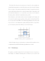
1.2.3.2 Fast Sweeping Method
The Fast Sweeping Method is an efficient iterative method which uses upwind
difference for discretization to solve the Eikonal equation [28]. The idea behind
Fast Sweeping is to “sweep” through the grid in certain directions, computing
the distance value for each grid point. The sweeping ordering follows a family of
characteristics of the corresponding Eikonal equation in a certain direction simultaneously. For example, in a two-dimensional domain, T at a grid point depends
on its neighbors in the following four ways:
• left and bottom neighbors,
• left and top neighbors,
• right and bottom neighbors,
• right and top neighbors.
Thus, for any point Xi,j in a domain, we compute the solution as being the minimum between the local discrete Eikonal equations solutions based on its neighbors
Xi±1,j , Xi,j±1 . Repeatedly, we sweep the whole domain along the diagonal and
anti-diagonal from top to bottom and from bottom to top. This sweeping idea is
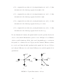
illustrated by solving the Eikonal equation in (-1,1):
dT = 1,
dx T (−1) = T (1) = 0.
(1.25)
From this point on, by a “sweep” we mean a computation in a certain direction
and by an “iteration” we mean a completed set of sweeps, i.e. four-direction sweeps
27
in 2D problems.
Let Ti = T (xi ) denote the values for the grid points −1 = x0 < x1 < . . . < xn = 1.
We solve (1.25) in different directions, using the discretized nonlinear system, based
on Godunov scheme (1.21):
max Dij−x T, −Dij+x T, 0 = 1,
-1
1
-1
(a)
T0 = Tn = 0.
(1.26)
1
1
-1
(b)
(c)
FIGURE 1.9. Sweeping in 2 directions
First, we have a sweep from left to right, enforcing the boundary condition at
x = 0. This is equivalent to following the directions emanating from x0 as shown
in Figure 1.9(a). We obtain the solution Ti = xi .
Secondly, we sweep from right to left, which means following the directions emanating from xn , as shown in Figure 1.9(b). We obtain the solution Ti = 1 − xi .
Since in 1-D there are only two directions of sweeping, i.e. left to right and right
to left, two sweeps are enough to compute the solution correctly. Thus, T at a
grid point Xi can be computed exactly from either its left or right neighbor,
T (Xi ) = min(Ti−1 , Ti+1 ) + h. Using the Godunov discretization scheme (1.26),
we obtain the continuous viscosity solution drawn in Figure 1.9(c):
Ti =



xi ,
−1 ≤ xi < 0

 1 − xi ,
28
0 ≤ xi ≤ 1.
n
, Ti is correctly computed based on its left neighbors dur2
n
ing the first sweep, while for i ≥ , Ti is correctly computed based on its right
2
neighbors during the second sweep. The Fast Sweeping algorithm is illustrated in
Notice that, for i ≤
Algorithm 2.
n
Remark 1.23. The first sweep satisfies the upwind-ing condition for 0 ≤ i ≤
2
n
and the second sweep for < i < n.
2
The most important point in the algorithm is that the upwind difference scheme
used in the discretization enforces that “the solution at a grid point be determined
by its neighboring values that are smaller” [28].
Algorithm 2 Fast Sweeping Algorithm
Consider S > diam(Ω);
Initialization:
Ti = 0 on Γ;
Ti = S, otherwise;
Iteration:
for i = 1 to n/2 do
Compute Ri solution of local Eikonal equation ;
end
for i = n − 1 to n/2 do
Compute Pi solution of local Eikonal equation ;
end
T̃i = min(Pi , Ri );
T = T̃ ;
29
Chapter 2
Sequential Fast Marching Methods
2.1
General Idea
The Fast Marching Method is very closely related to Dijkstra’s algorithm, a wellknown algorithm from the 1950’s for computing the shortest path on a network.
Dijkstra’s algorithm is widespread, from Internet routing applications to navigation
system applications. To explain the connection, consider a network with a cost
assigned to each node as in Figure 2.1:
(a)
(b)
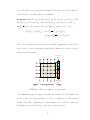
FIGURE 2.1. Dijkstra algorithm for finding the shortest path from Start to Finish
The basic idea of Dijkstra’s method [7] is as follows:
1. Put the starting point in a set called “Accepted”.
2. Call the grid points which are one link away from the Start “Neighbors”.
3. Compute the cost of reaching each of these “Neighbors”.
30
4. The smallest cost of these Neighbors must be the correct cost. Remove it
from “Neighbors”, call it “Accepted” and return to step 2, until all points
are labeled “Accepted”.
The algorithm orders the way in which the points are accepted, from the known
costs (the starting point) all the way to the finish. The method is a one-pass
method, each point being touched essentially only once. Note that it is not guaranteed that the method converges to the optimal solution.
The Fast Marching Methods use upwind difference operators to approximate the
gradient, but retains the Dijkstra idea of a one-pass algorithm.
Tsitsiklis was the first to develop a Dijkstra-like method for solving the Eikonal
equation. Addressing a trajectory optimization problem, he presented a first-order
accurate Dijkstra-like algorithm in [27]. Later Sethian and Osher [18, 22, 23, 24]
developed the idea and produced the Fast Marching Methods.
For solving equation (1.1), assume that n = 2 and F (x) > 0. All the results obtained in this case can be generalized to the 3-dimensional case.
The central idea behind the Fast Marching Methods is to systematically construct
the solution of (1.1) outward from the smallest values of T to its largest ones, stepping away from the boundary condition in a downwind direction. The algorithm
is initialized by tagging the points of the domain as:
• far away nodes: Ti,j = +∞ - T has never been calculated,
• accepted nodes: Ti,j = 0 is given,
• narrow band nodes: these are the neighbors of the accepted points.
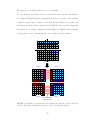
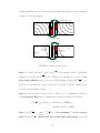
As it can be seen in Figure 2.2, the yellow-orange region, representing the narrow
band points, separates the accepted nodes from the far away nodes. The algorithm
is mimicking the front evolution step by step:
31
accepted values
upwind side
narrow band
values
downwind side
far away values
FIGURE 2.2. Far away, narrow band and accepted nodes
• sweep the front ahead by considering the narrow band points,
• march this narrow band forward, freezing the values of existing points and
bringing new points into the narrow band.
The key is in selecting which grid point in the narrow band to update. The algorithm will stop when all the nodes become accepted.
2.2
Fast Marching Algorithm Description
Let Ω be the rectangular domain (0, 1) ×(0, 1) of R2 . Given the discretization steps
1
1
∆x = , ∆y =
> 0, we denote by Tij the value of our numerical approximation
N
M
of the solution at (xi , yj ) = (i∆x, j∆y), i = 0, . . . , N, j = 0, . . . , M. Similarly, Fi,j
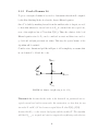
represents the value of F at node (xi , yj ).
We define the neighbors of a grid point (xi , yj ):
Definition 2.1. The set of neighboring nodes of a grid point X = (xi , yj ) is:
V (X) = {(xi+1 , yj ), (xi−1 , yj ), (xi , yj+1), (xi , yj−1)} ,
32
for 1 ≤ i ≤ N − 1 and 1 ≤ j ≤ M − 1.
Remark 2.2. The definition of V (X) has to be adapted for i = 0 or j = 0 and
i = N or j = M, by eliminating the appropriate points.
These are the nodes appearing in the stencil of the finite difference discretization.
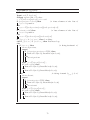
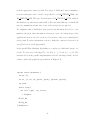
The Fast Marching algorithm is presented in Algorithm 3.
Algorithm 3 Fast Marching algorithm
Initialization:
Set T = 0 for accepted nodes.
Tag all neighbors of accepted nodes, that are not accepted as narrow band.
Compute T for all narrow band nodes.
Set T = +∞ for the rest of the nodes.
Main Cycle:
repeat
Let A be the smallest T from all narrow band nodes
Add node A to accepted
Remove A from narrow band
Tag as narrow band all neighbors of A that are not accepted
for all y ∈ V (A) do
if y is in far away then
Remove neighbor from far away
Add it to narrow band set.
end
if y is in narrow band then
Update Ti,j by solving the local Eikonal equation (1.22) at Xi,j .
end
end
until all nodes are accepted ;
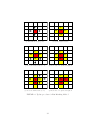
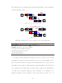
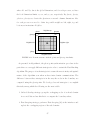
In Figure 2.3, the Fast Marching algorithm is graphically illustrated. In order to
have a better understanding of the algorithm, we consider the case of an isolated
accepted node in the domain and we replace the network grid representation with
the table format. The algorithm steps are:
• start from the accepted node X, shown as a red cell in Figure 2.3(a)
33
X
C
B X D
A
(a) Start with an accepted point
(b) Update neighbors values
C
B X D
A
C
B X D
A
(c) Choose the smallest value (i.e. A)
(d) Freeze value of A, update its neighbors
C
B X D
A
C
B X D
A
(e) Choose the smallest value (i.e. D)
(f) Freeze value of D, update its neighbors
FIGURE 2.3. Update procedure for Fast Marching Method
34
• march ”downwind” from X, solve the local Eikonal equation (1.22) at all
neighbors Y ∈ V (X). T (Y ) for all Y ∈ V (X), represented by yellow-orange
cells in Figure 2.3(b), are narrow band points.
• consider the neighbor A of X with the smallest T and tag it as accepted (see
Figure 2.3(c) and 2.3(d)). Due to the upwinding property of the difference
operator used in equation (1.22), T (A) is now correct (up to the discretization
error).
• tag the neighbors of A as narrow band points (yellow-orange cells in Figure
2.3(d)).
• choose the narrow band point with the smallest T , i.e. D (see Figure 2.3(e)
and 2.3(f))
• repeat the algorithm until all the nodes become accepted.
Remark 2.3. Ti,j is determined only by those neighboring nodes of smaller T .
2.3
Convergence
Theorem 2.4. As the mesh size goes to zero, i.e. ∆x → 0 and ∆y → 0, the
numerical solution built by the Fast Marching Methods converges to the viscosity
solution of (1.1).
Proof. The proof is performed in two steps, through the following lemmas.
Lemma 2.5. The solution of the discrete Eikonal equation converges toward the
viscosity solution, as the mesh sizes go to zero [3].
Lemma 2.6. The sequence built by Fast Marching Methods converges to the solution of discrete Eikonal equation.
35
2.3.1
Proof of Lemma 2.5
The proof is borrowed from Barles and Souganidis [3].
Consider an approximation scheme of the form:
S(ρ, x, uρ ) = 0 in Ω̄,
(2.1)
where S : R+ × Ω̄ × L∞ (Ω̄) → R is locally bounded, L∞ (Ω̄) is the space of bounded
functions defined on Ω̄ and uρ is the solution of (2.1).
Let u be the viscosity solution of the Hamilton Jacobi equation: H(x, Du) = 0 on
Ω and u = φ on ∂Ω.
If this scheme is monotone, stable and consistent with the Hamilton-Jacobi equations, it converges to the solution of (1.1). For this, we need to recall some results
from [3].
Definition 2.7 (Monotonicity). The scheme S is monotone if and only if it satisfies:
S(ρ, x, u) ≤ S(ρ, x, v), if u ≥ v, ∀ ρ ≥ 0, x ∈ Ω̄ and u, v ∈ L∞ (Ω̄)
(2.2)
The purpose of the scheme S is to approximate the Hamilton-Jacobi equations
and thus the monotonicity condition for S is equivalent to the ellipticity condition
for H for the Hamilton-Jacobi equation H(x, ∇u) = 0 in Ω̄. That is, for all M, N,
if for all x ∈ Ω̄, H(x, M) ≤ H(x, N), then M ≥ N. This property assures some
maximum principle type property for the scheme.
Definition 2.8 (Stability). The scheme S is stable if and only if:
∀ ρ > 0, ∃ a uniformly bounded solution uρ ∈ L∞ (Ω̄) such that (2.1) holds. (2.3)
The bound is independent of ρ.
36
The scheme is stable in the sense that for all points of space discretization, the
solution exists and has a (lower and upper) bound. Moreover, it is independent
of discretization step (the information propagates from the smaller value of T to
larger values).
Definition 2.9 (Consistency). The scheme S, defined in (2.1), is consistent, i.e.
∀ x ∈ Ω̄ and φ ∈ C ∞ (Ω̄)
lim sup
ρ→0
y→x
ξ→0
S(ρ, y, φ + ξ)
≤ lim supH(x, D 2 φ(x))
ρ
y→x
(2.4)
S(ρ, y, φ + ξ)
≥ lim inf H(x, D 2φ(x))
y→x
ρ
(2.5)
and
lim inf
ρ→0
y→x
ξ→0
Definition 2.10 (Strong Uniqueness). Consider the solution u ∈ L∞ (Ω̄) of the
Hamilton-Jacobi equation:
H(x, ∇u) = 0 in Ω̄
(2.6)
If for any x ∈ Ω, one has that u(x) = lim sup u(y), then u is the upper semiy→x
continuous envelope of the solution of equation (2.6). Similarly, v(x) = lim inf v(y)
y→x
is the lower-semi-continuous envelope of the solution of equation (2.6)
Lemma 2.11 (Strong Uniqueness Property). In the setting of the previous definition, if u and v are the upper-semi-continuous envelope, and the lower-semicontinuous envelope of the solution of (2.6), respectively, then
u ≤ v on Ω̄.
(2.7)
The following theorem is the Barles and Souganidis convergence result published
in [3] pg. 275-276.
37
Theorem 2.12. Assume that (2.2), (2.3), (2.4), (2.5) and the hypothesis of Lemma
(2.11) hold. Then, as ρ → 0, the solution uρ of (2.1) converges locally uniformly
to the unique continuous viscosity solution u of (2.6).
Proof. The proof follows the steps and arguments presented in [3], pg. 275-276,
[2], pg. 576-577 and [5].
Consider uρ satisfying (2.1) and let ū, u ∈ L∞ (Ω̄) be defined as:
ū = lim sup uρ(y)
y→x
ρ→0
(2.8)
ρ
u = lim
inf u (y)
y→x
.
ρ→0
Assume that ū, u are sub and super viscosity solutions of (2.6). Then, based on
their definitions, ū ≥ u. Since ū is the upper-semi-continuous (usc) and u is the
lower-semi-continuous (lsc) envelope of solution of (2.1), Lemma (2.11) implies that
ū ≤ u. Hence, we can write that ū = u ≡ u.
Since the upper semi-continuous solution ū and lower semi-continuous solution
u are equal, Lemma (2.11) assures that u is the unique continuous solution of
Hamilton-Jacobi equation (2.6). Using (2.8), one gets that uρ converges locally
uniformly to u.
Now let us prove that ū, u are the viscosity sub-solution and super-solution of
(2.6). We only present the case of ū being the sub-solution of (2.6).
Let x0 be a local maximum of ū − φ on Ω̄, for some φ ∈ C ∞ (Ω̄). We assume
that x0 is the unique maximum point of ū − φ in B(x0 , r), for some r > 0, such
that ū(x0 ) = φ(x0 ) inside the ball B(x0 , r) and φ ≥ 2 supρ kuρ k∞ outside the ball
B(x0 , r). In some neighborhood of x0 , with x 6= x0 , we have:
ū(x) − φ(x) ≤ 0 = ū(x0 ) − φ(x0 ) in B(x0 , r), for some r > 0.
38
By Lemma A.3, pg. 577 of Barles and Perthame in [2], there exist sequences yn ∈ Ω̄
and ρn ∈ R+ such that for n → ∞
yn → x0 , ρn → 0, uρn (yn ) → ū(x0 ) and
(2.9)
yn is a global maximum point of uρn (.) − φ(.).
Hence for yn → x0 and all x ∈ B(x0 , r) we have
uρn (yn ) − φ(yn ) ≤ 0 = uρn (x0 ) − φ(x0 ).
(2.10)
In [5], Crandall and Lions remarked that by replacing φ(yn ) with φ(yn ) + ξn , where
ξn → 0, there exists a sequence still denoted yn of local maximum points of uρn − φ
converging to x0 . Thus, relation (2.10) becomes:
uρn (yn ) ≤ φ(yn ) + ξn , for all x ∈ Ω̄.
Applying the monotonicity property (2.2) of scheme S to uρn (yn ) ≤ φ(yn ) + ξn one
gets:
S(ρn , yn , φ + ξn ) ≤ S(ρn , x, uρn ).
By definition of the uρn , S(ρn , x, uρn ) = 0, and so:
S(ρn , yn , φ + ξn ) ≤ 0.
(2.11)
Taking the limit of (2.11) and using the consistency property (2.5) of S, one gets:
S(ρn , yn , φ + ξn )
n
ρn
S(ρ, y, φ + ξ)
≥ lim
inf
y→x0
ρ
ρ→0
0 ≥ lim inf
ξ→0
≥ lim inf H(x0 , D 2 (φ(x0 )).
y→x0
Since ū(x0 ) = φ(x0 ), lim inf H(x0 , D 2 (φ(x0 )) ≤ 0 and ū is the sub-solution of
y→x0
(2.6).
39
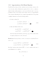
Now, we have all the tools to prove Lemma 2.5 for our numerical scheme.
In our case, the numerical approximation scheme will satisfy:


 gij (D −x Ti,j , D +x Ti,j , D −y Ti,j , D +y Ti,j ) = 0, x ∈ Ω

 T (x) = 0,
(2.12)
x ∈ Γ,
where gij (D −x Ti,j , D +x Ti,j , D −y Ti,j , D +y Ti,j ) is computed as
q
1
max(D −x Ti,j , D +x Ti,j )2 + max(D −y Ti,j , D +y Ti,j )2 −
.
Fi,j
The discretization ρ represents a pair (∆x, ∆y) of space discretization steps, uρ =
Ti,j is a function defined on ∆ρ = {(xi , yi), i = 0, . . . , N, j = 0, . . . , M} ∩ Ω̄ and
for all x ∈ Ω̄, we define u and ū as:
u = lim inf
inf
uρ (y)
ū = lim sup
sup
uρ (y).
η→0 y∈B(x,η)∩∆ρ
0<ρ<η
and
η→0 y∈B(x,η)∩∆ρ
0<ρ<η
Our scheme is monotone, i.e. if U ≥ V , then for all i, j we have
gij (D −x Ui,j , D +x Ui,j , D −y Ui,j , D +y Ui,j ) ≤ gij (D −x Vi,j , D +x Vi,j , D −y Vi,j , D +y Vi,j ).
The scheme is stable since uρ has its minima in ∂Ω and is bounded below by a
constant independent of ρ, which is the minimum value on ∂Ω.
The scheme is consistent with the Hamilton-Jacobi equation (2.6) as, for each i, j,
gij (a, a, b, b) =
√
a2 + b2 −
1
, for all a, b ∈ R.
Fij
We can also prove, as in [3], that ū and u are the sub-solution and the supersolution of equation (2.6) respectively and that u ≤ ū on ∂Ω.
Since our approximation scheme satisfies all the assumptions made in the hypothesis of Theorem 2.12, we can apply Theorem 2.12 to prove that the solution of
the discrete Eikonal equation converges toward the viscosity solution, as the mesh
sizes go to zero.
40
2.3.2
Proof of Lemma 2.6
To prove convergence Lemma 2.6 we need to demonstrate that the field computed
by the Fast Marching Methods solves the discrete Eikonal equation.
Since T is built by marching forward from the smallest value to largest, we need
to show that whenever a narrow band node Xi,j is converted into an accepted one,
none of its neighbors has a T less than T (Xi,j ). Thus, the solution of the local
Eikonal equation at node Xi,j can be considered as exact and there is no need to
go back and readjust previously set values. This way, the upwind nature of the
algorithm will be satisfied.
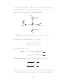
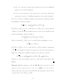
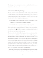
Consider a two dimensional grid like in Figure 2.4. For simplicity, we assume that
in our domain N = M and ∆x = ∆y.
Xi+1, j
nb
acc
Xi,j-1
Xi,j
Xi, j+1
Xi-1,j
FIGURE 2.4. Matrix of neighboring nodes of Xi,j
Theorem 2.13. Assume that the nodes in the domain Ω are partitioned into accepted, narrow band and far away nodes. By construction, we have that for any
two nodes Y and Z, if Y has become accepted before Z, then T (Y ) ≤ T (Z).
Assume that Xi,j−1 is the narrow band point with the smallest T . The algorithm
will label Xi,j−1 as accepted and start to compute the neighboring nodes that are
41
not accepted.
Furthermore, assume that:
• F ∈ Lip(Rn ) ∩ L∞ (Rn ), with Lipschitz constant Lf .
• F (x) > 0, for x ∈ Ω and Fmin = min F (x) > 0,
Ω
• the Courant Friedrichs Lewy-like (CFL) condition holds true [6]:
√
Fmin
.
∆x ≤ ( 2 − 1)
Lf
(2.13)
Then we have the upwind condition satisfied:
Ti,j−1 ≤ Ti,j ≤ Ti,j−1 +
∆x
.
Fi,j
(2.14)
Remark 2.14. The above theorem shows that the value of the smallest node in the
narrow band can be computed exactly at the next iteration. An approximate value
is considered to be exact, within the consistency error of the scheme, if at the next
iterations of the algorithm we cannot obtain a lower value [6].
Remark 2.15. We can make the assumptions that Ti+1,j ≤ Ti−1,j and Ti,j−1 ≤
Ti,j+1, without loss of generality, up to two mirror symmetries of the domain.
Proof. (Theorem 2.13) To compute T at Xi,j we distinguish the following cases
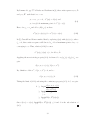
[22, 23, 6]:
Case 1: one of the Xi,j neighbors is accepted,
Case 2: two of the Xi,j neighbors are accepted,
Case 3: three of the Xi,j neighbors are accepted.
Case 4: all the Xi,j neighbors are accepted.
42
Case 1:
Suppose that only one of Xi,j ’s neighbors is accepted. Up to a rotation, we can
assume without loss of generality that this node is Xi,j−1. All the other possible
situations will be treated in a similar way. This case is graphically illustrated in
Figure 2.5.
Xi+1, j
nborfar
nb
acc
Xi,j-1
nborfar
Xi,j
Xi, j+1
nborfar
Xi-1,j
FIGURE 2.5. Node Xi,j has only one accepted neighbor
Note also that Ti,j < Ti−1,j , Ti,j < Ti,j+1 and Ti,j < Ti+1,j , since these three
neighbors are either far away or narrow band nodes and Xi,j is the narrow band
node with smallest T . Therefore we have that:
D −x Ti,j ≥ 0,
D +x Ti,j ≥ 0,
D −y Ti,j ≤ 0,
D +y Ti,j ≥ 0.
and equation (1.22) becomes:
max(D −x Ti,j , 0)
2
1
2
Fi,j
2
1
D −x Ti,j = 2 .
Fi,j
+ (max(0, 0))2 =
Using the definition (1.20) of the finite difference operator D −x Ti,j , we obtain:
Ti,j − Ti,j−1
∆x
43
2
=
1
,
2
Fi,j
(2.15)
and
Ti,j = Ti,j−1 ±
∆x
.
Fi,j
Since we assumed that Xi,j−1 is the only accepted neighbor of Xi,j , we have that
∆x
.
Ti,j > Ti,j−1. Therefore: Ti,j = Ti,j−1 +
Fi,j
∆x
In the case of only one accepted node, we proved that Ti,j−1 ≤ Ti,j = Ti,j−1 +
.
Fi,j
Case 2:
Suppose that two neighbors of Xi,j are accepted. From hypothesis we know that
node Xi,j−1 is one of the accepted neighbors. We have three ways of positioning
the other accepted node: at the top, at the bottom or at the right of Xi,j . Let us
study the case of top node and the case of right node.
2.1: Up to a rotation in the domain, we can assume without loss of generality
that the accepted nodes are Xi+1,j and Xi,j−1, with Ti+1,j < Ti,j−1 . In this
case the other two neighbors of Xi,j are narrow band or far away nodes, as
presented in Figure 2.6. We should remark that Ti,j < Ti,j+1, Ti,j < Ti−1,j ,
since Xi,j is the narrow band node with the smallest T .
Xi+1, j
acc
nb
acc
Xi,j-1
Xi,j
nb orfar
Xi, j+1
nborfar
Xi-1,j
FIGURE 2.6. Node Xi,j has the neighbors Xi,j−1 and Xi+1,j accepted
44
In this case the finite difference operators are:
D −x Ti,j ≥ 0,
D +x Ti,j ≥ 0,
D −y Ti,j ≤ 0,
D +y Ti,j ≤ 0.
and equation (1.22) becomes:
max(D −x Ti,j , 0)
1
2
Fi,j
2
2
1
D −x Ti,j + D +y Ti,j = 2 .
Fi,j
2
+ max(0, D +y Ti,j )
2
=
Using the finite difference operators D −x Ti,j and D +y Ti,j , we get:
Ti,j − Ti,j−1
∆x
2
+
Ti+1,j − Ti,j
∆y
2
=
1
,
2
Fi,j
and
∆x2
(Ti,j − Ti,j−1) + (Ti+1,j − Ti,j ) = 2 ,
Fi,j
2
2
(2.16)
Solving the quadratic equation in Ti,j we get:
q
2
2
Ti,j−1 + Ti+1,j ± 2 ∆x
2 − (Ti,j−1 − Ti+1,j )
Fi,j
Ti,j =
.
2
(2.17)
Since Xi,j−1, Xi+1,j ∈ A(Ω), Ti,j > Ti,j−1 , Ti,j > Ti+1,j , and therefore
Ti,j >
Ti−1,j +Ti,j+1
.
2
Hence we consider only the solution of (2.17) involving
the “+” sign:
Ti,j−1 + Ti+1,j
Ti,j =
q
2
− (Ti,j−1 − Ti+1,j )2
+ 2 ∆x
F2
i,j
2
.
Since Ti,j is the solution of equation (2.16), we can rewrite it as:
(Ti,j − Ti,j−1)2 =
∆x2
− (Ti+1,j − Ti,j )2 ,
2
Fi,j
and therefore
(Ti,j − Ti,j−1 )2 ≤
45
∆x2
.
2
Fi,j
(2.18)
Since both sides of the above inequality are positive, we can take the square
root and get
Ti,j − Ti,j−1 ≤
∆x
.
Fi,j
(2.19)
Now, we can conclude that:
Ti,j−1 ≤ Ti,j ≤ Ti,j−1 +
∆x
.
Fi,j
In order to complete the proof for this case, we need to show that the expression that appears under the square root in the calculation of Ti,j as a
function of two of its neighbors, in equation (2.18), can never be negative .
Since node Xi+1,j was accepted before node Xi,j−1, we know that Ti,j−1 ≤
∗
Ti+1,j . In this setting, Ti,j
was first computed based on Xi+1,j and following
the arguments from case 1, we can say that:
∗
Ti+1,j ≤ Ti,j
≤ Ti+1,j +
∆x
.
Fi,j
∗
Since Xi,j−1 becomes accepted before Xi,j , we have that Ti,j−1 ≤ Ti,j
.
From all of these, we deduce that:
∗
Ti+1,j ≤ Ti,j−1 ≤ Ti,j
≤ Ti+1,j +
∆x
,
Fi,j
which implies that
0 ≤ Ti,j−1 − Ti+1,j ≤
∆x
.
Fi,j
(2.20)
Therefore, when we compute Ti,j at the current iteration, from equation
(2.18), the quantity under the square root becomes:
2∆x2 ∆x2
∆x2
2∆x2
2
− (Ti,j−1 − Ti+1,j ) ≥
− 2 = 2 ≥ 0.
2
2
Fi,j
Fi,j
Fi,j
Fi,j
2.2: Up to a rotation in the domain, we can assume without loss of generality
that the accepted nodes are Xi,j+1 and Xi,j−1, with Ti,j+1 < Ti,j−1 . In this
46
case the other two neighbors of Xi,j are narrow band or far away nodes, as
presented in Figure 2.7. We should remark that Ti,j < Ti+1,j , Ti,j < Ti−1,j ,
since Xi,j is the narrow band node with the smallest T .
Xi+1, j
nborfar
nb
acc
Xi,j-1
acc
Xi, j+1
Xi,j
nborfar
Xi-1,j
FIGURE 2.7. Node Xi,j has the neighbors Xi,j−1 and Xi,j+1 accepted
For this situation, the finite difference operators are:
D −x Ti,j ≥ 0,
D +x Ti,j ≤ 0,
D −y Ti,j ≤ 0,
D +y Ti,j ≥ 0.
and equation (1.22) becomes:
1
2
Fi,j
2
1
max(D −x Ti,j , −D +x Ti,j ) = 2 .
Fi,j
max(D −x Ti,j , −D +x Ti,j )
2
+ (max(0, 0))2 =
Using the finite difference operators D −x Ti,j and D +x Ti,j , we get:
2
Ti,j − Ti,j−1
1
= 2
∆x
Fi,j
2
Ti,j − Ti,j+1
1
= 2 .
∆x
Fi,j
Since Ti,j ≥ Ti,j−1 and Ti,j ≥ Ti,j+1, this case is equivalent to solving the
local Eikonal equation for Ti,j in first and in second quadrant, and taking the
47
minimum of the solutions:
Ti,j = min (Ti,j+1 +
∆x
∆x
, Ti,j−1 +
).
Fi,j
Fi,j
Repeating the first case steps, we conclude that:
Ti,j+1 ≤ Ti,j−1 ≤ Ti,j ≤ Ti,j−1 +
∆x
∆x
≤ Ti,j+1 +
.
Fi,j
Fi,j
Case 3 and 4, where three or all the Xi,j ’s neighbors are accepted, are similar
to the previous cases, since the finite differences take the smallest values in each
coordinate direction.
Remark 2.16. We should remark that the proof of Theorem 2.13 provides a constructive solution for the local Eikonal equation at Xi,j . In the implementation, we
notice that it is more efficient to solve the four variants of equation (2.15) and
(2.16) and take the minimum of these real solutions.
Convergence of Fast Marching
At each step of the algorithm the size of the accepted nodes set grows by 1. We
can apply Theorem 2.13 iteratively using induction on the number of iterations of
the algorithm.
During first iteration, if node Xi,j−1 is accepted, then its value is known and ini∆x
, which satisfies relation (2.14)
tialized with Ti,j−1 = 0 and we have Ti,j ≤ 0 +
Fi,j
and therefore Theorem 2.13 holds true.
At the n-th step of the algorithm, the induction hypothesis implies that, at each
iteration, the T ’s at the nodes in the narrow band are greater than the ones at the
nodes labeled as accepted. And thus Theorem 2.13 can be applied.
In conclusion, the upwind nature of the numerical scheme is satisfied since T at
the node labeled as accepted, at every iteration, is exact, i.e. it cannot be improved
on the same grid [22].
48
Chapter 3
Parallel Fast Marching Methods
In the previous sections we saw that Fast Marching Methods are inherently sequential and hence not straightforward to parallelize and implement on today’s
supercomputers. Parallelizing Fast Marching Methods is a step forward for employing the Level Set Methods on parallel supercomputers.
3.1
General Idea
The idea behind the distributed implementation of the Fast Marching Methods is
to divide the whole computational grid between processors, giving each processor
access to only its own sub-domain, and use message passing strategy to communicate between different processors (more details about parallel computing can be
found in section 4.3). This approach has its own drawbacks:
• when the grid is simply split between processors, in some cases there is no
longer enough data to update all the points in each sub-domain,
• we cannot preserve the upwind nature of the numerical scheme for the whole
domain just in one pass,
• communication through message passing is really expensive, since it requires
a lot of time for data transmissions.
The efficiency of the parallel algorithms depends on the required amount of communication between sub-domains, i.e. how often boundary nodes change status,
and our ability to preserve the upwind structure during the algorithm execution.
49
All of the above are main obstacles for good scalability.
To overcome these problems, ghost-zones with ghost points are used. Ghost-zones
are additional (duplicated) grid points which are added to each processor and they
contain necessary data to advance to the next iteration. Hence, we expand each
sub-domain by adding 1 layer of ghost nodes. All ghost-nodes of a sub-domain form
the ghost-zone or overlap of that sub-domain. Figure 3.1 illustrates the particular
decomposition of a two dimensional 10 × 10 grid into four sub-domains.
One CPU
CPU 2
CPU 3
CPU 0
Inter-subdomains
communication
CPU 1
FIGURE 3.1. Domain decomposition in sub-domains, the dark blue cells are the ghost
cells, the dashed line delimits the ghost-zone for the top right sub-domain
50
The dashed line shows how the ghost-zone is formed for the top-right subdomain. In the same manner, we formed the ghost-zones for the other sub-domains.
The second part of the picture presents the sub-domain decomposition and indicates in dark blue the ghost-zone for each sub-domain. After decomposition, each
sub-domain has dimension 6 × 6, because there are an extra row and column for
the ghost points to make sub-domains interaction possible.
In two-dimension, a sub-domain can have at most four neighbor sub-domains, and
also at most four ghost-regions, depending on the position on the global grid. Figure 3.2 (reproduced from PETSc User Manual [19]) illustrates the ghost points
for process six of a two-dimensional, regular parallel grid. Each box represents a
process; the ghost points for the sixth process are shown in gray.
Proc 6
Proc 0 Proc 1
FIGURE 3.2. Ghost points for a particular process
In the following sections, we address the above issues and the way that we chose
to implement the parallel Fast Marching algorithm in more details.
3.2
Notations
We partition our initial domain Ω in Ns sub-domains. In order to keep the notation simple, we commit the following abuse of notation: by Ω, we denote both
51
the domain and the discretized domain, i.e (0, 1) × (0, 1) and {0, 1, . . . , N} ×
{0, 1, . . . , M}.
We use k, 1 ≤ k ≤ Ns , to denote the sub-domain index and by Ωk we refer to the
sub-domain k.
Definition 3.1. For a sub-domain Ωk we denote its boundary by ∂Ωk .
The sub-domain Ωk together with its ghost-points form the so called extended subdomain, denoted by Ω̃k .
Any point in the domain is denoted by Xi,j , where 0 ≤ i ≤ N and 0 ≤ j ≤ M
are the row and column indexes. When decomposing the domain in sub-domains,
it is necessary to distinguish between neighbors in the sub-domain and neighbors
that are ghost-points.
Definition 3.2. Consider a sub-domain Ωk and a node Xi,j ∈ Ωk , we define
• the set of neighbors of Xi,j in Ωk as:
D(Xi,j ) = {Y ∈ {Xi+1,j , Xi−1,j , Xi,j+1, Xi,j−1}
T
Ωk } ,
• the set of ghost neighbors of Xi,j as:
G(Xi,j ) = {Y ∈ {Xi+1,j , Xi−1,j , Xi,j+1 , Xi,j−1}\Ωk } .
Definition 3.3. The ghost-zone of a sub-domain contains all the ghost-nodes of
that sub-domain and it is denoted G(Ωk ), k = 1, . . . , Ns , where Ns is the number
of sub-domains.
Definition 3.4. For any node Xi,j of the grid, we define the neighbors set as
V (Xi,j ) = D(Xi,j ) ∪ G(Xi,j ).
52
i,j-1
i+1,j
i,j-1
i,j
i,j
i,j+1
i-1,j
i,j+1
i-1j
(a) Node inside a sub-domain
(b) Node on a row boundary
i+1,j
i,j
i,j-1
i-1,j
i+1,j
i,j-1
i,j
i,j+1
i,j+1
i-1,j
(c) Node on a column boundary
(d) Node on a corner boundary
FIGURE 3.3. Neighbors of Xi,j
In Figure 3.3, the sub-figures illustrate the difference between the neighbors and
the ghost neighbors, based on a typical situation.
Thus, the sets of neighbors and ghost neighbors of Xi,j are:
• figure 3.3(a): D(Xi,j ) = {Xi+1,j , Xi−1,j , Xi,j+1, Xi,j−1 } and G(Xi,j ) = {0},
• figure 3.3(b): D(Xi,j ) = {Xi−1,j , Xi,j−1 , Xi,j+1} and G(Xi,j ) = {0},
• figure 3.3(c): D(Xi,j ) = {Xi+1,j , Xi−1,j , Xi,j−1 } and G(Xi,j ) = {Xi,j+1 },
• figure 3.3(d): D(Xi,j ) = {Xi,j+1, Xi−1,j } and G(Xi,j ) = {Xi,j−1, Xi+1,j }.
53
Remark 3.5. Again, we commit an abuse of notation, since special care has to be
applied when Xi,j is at the boundary of Ωk . We let the reader distinguish between the
indices of a ghost node and a node in the domain (X0,0 ∈ ∂Ωk and X−1,0 ∈ G(X0,0 ),
but 0 ≤ i ≤ N).
Definition 3.6. By A(Ωk ), NB(Ωk ) and FA(Ωk ) we denote the sets of accepted,
narrow band, and far away nodes over the sub-domain Ωk .
We also define:
• the set of accepted nodes over the boundary of domain Ωk as:
A(∂Ωk ) = A(Ωk ) ∩ ∂Ωk ,
• the set of narrow band nodes over the boundary of domain Ωk as:
NB(∂Ωk ) = NB(Ωk ) ∩ ∂Ωk ,
• the set of far away nodes over the boundary of domain Ωk as:
FA(∂Ωk ) = FA(Ωk ) ∩ ∂Ωk .
3.3
Parallel Fast Marching Algorithm
The main idea of the parallel algorithm is to perform Fast Marching on the subdomains, update the boundary values at the interfaces and restart the algorithm
until convergence is achieved. To update the boundary values at the interfaces we
need to preserve the upwind structure of the numerical scheme and to synchronize
the ghost-zones at each iteration.
The parallel Fast Marching algorithm performs iteratively, the steps presented in
Algorithm 4, until convergence is achieved.
54
Algorithm 4 Parallel Fast Marching algorithm
repeat
Compute Tkn (Xi,j ), ∀Ωk , ∀Xi,j ∈ Ωk , k = 0, . . . , Ns using Fast Marching on the
sub-domains (local FM)
Ghost points synchronization
( /* Exchange and update the boundary data at the interfaces */)
until convergence conditions are satisfied ;
3.3.1
Ghost Points
The ghost-zones synchronization is not trivial, since it should preserve the upwind
nature of the discretization scheme. The steps of the ghost-zones synchronization
procedure are presented in Algorithm 5.
Algorithm 5 Ghost-zones Synchronization procedure
begin
n+ 1
1. ∀Ωk , Xi,j ∈ ∂Ωk , compute Tk 2 (Xi,j ) as the solution of the local Eikonal
equation at Xi,j ∈ Ω̃k
2. reassign the flags
n+ 1
3. save the minimum of all Tk 2 for Xi,j ∈ ∂Ωk and use it to update the flags
in Ωk .
end
Remark 3.7. To avoid confusions in the parallel implementation, when we refer
to the value of a certain point, we need to specify its sub-domain and also the
iteration during which it was computed. Therefore, let Tkn (Xi,j ) be the T at node
Xi,j , obtained during nth iteration, at the end of local Fast Marching algorithm, in
n+ 21
sub-domain Ωk , and Tk
(Xi,j ) be the T at node Xi,j in sub-domain Ωk , obtained
after the ghost-points synchronization.
Consider a domain with the starting nodes in opposite corners. These nodes are
initialized as accepted nodes at the beginning of the Fast Marching algorithm. Let
us consider the particular decomposition of the domain in two sub-domains, each
including one of the accepted nodes, as illustrated in Figure 3.4. In the following,
55
for this particular case, we describe how the synchronization procedure works step
by step for each sub-domain.
min ghost value = X
min ghost value = Y
(a) After Local FM
FA
T>X
Level line
T= X
Kept (A)
T<Y
Level line
T= Y
Kept (A)
T<X
T>Y
FA
(b) After Ghost Update
FIGURE 3.4. Ghost points update
n+ 21
Step 1: for all Ωk and all X ∈ ∂Ωk , let Tk
n+ 21
equation at X in Ω̃k . If Tk
be the solution of the local Eikonal
(Xi,j )k < Tkn (Xi,j ), we say that Xi,j is a node with
n+ 21
ghost point influence in Ωk (colored in blue in Figure 3.4(a)). If Tk
(Xi,j ) =
Tkn (Xi,j ), we say that Xi,j is an accepted node, and its T will not change in Ωk
(colored in red in Figure 3.4(a)).
Step 2: for all Ωk and for any node Xi,j ∈ ∂Ωk , we do a comparison so that we
can reassign the flags and reconstruct the accepted and narrow band sets:
n+ 21
if Tk
(Xi,j ) ≤ Tkn (Xi,j ) then tag Xi,j ∈ NB(Ωk )
otherwise tag Xi,j ∈ A(Ωk ).
n+ 21
Step 3: let Tk
=
n+ 21
band. We use Tk
min
Y ∈NB(∂Ωk )
n+ 21
Tk
(Y ) be the minimum T on the narrow
to update the flags of the whole sub-domain, i.e. for all
56
Xi,j ∈ Ωk :
n+ 21
if Tk
n+ 21
if Tk
n+ 21
if Tk
n+ 21
In Figure 3.4(b), Tk
n+ 21
(Xi,j ) < Tk
n+ 21
(Xi,j ) = Tk
n+ 21
(Xi,j ) > Tk
,
then Xi,j ∈ A(Ωk )
,
then Xi,j ∈ NB(Ωk )
,
then Xi,j ∈ FA(Ωk ).
n+ 1
= X for the left sub-domain and Tk+12 = Y for the right
sub-domain. The red region represents the accepted nodes , the yellow region represents the narrow band and the white one is for the far away nodes.
As presented in Algorithm 4 the ghost point synchronization procedure is the
part where we can apply different strategies in order to restart the Fast Marching
algorithm. The purpose of such strategies is to assure the monotonicity and upwind nature of the scheme even when we have inter-domain communications. The
difference between strategies is in the way the boundary is computed using the
ghost-points. We will describe these strategies in detail in Chapter 4.
3.4
Convergence
First let us remark that:
Remark 3.8. For any iteration n, the following hold true:
• for any two nodes Xi,j ∈ NB(Ωk ) and Xr,c ∈ A(Ωk ), we have
Tkn (Xi,j ) > Tkn (Xr,c ), for 0 ≤ r, i ≤ M and 0 ≤ c, j ≤ N,
• if Xi,j ∈ NB(Ωk ) with Tkn (Xi,j ) =
min
Y ∈NB(Ωk )
Tkn (Y ), then, at the next itera-
tion, Xi,j ∈
/ NB(Ωk ) and Xi,j ∈ A(Ωk ) (it will be the next node labeled as
accepted).
In the ghost-zone synchronization procedure, we reconstruct the narrow band
of each sub-domain as a function of minimum/maximum values of the boundary
57
nodes. We have to prove that the minimum T over the narrow band cannot be
decreased if we do not have ghost-nodes influence.
Proposition 3.9. For all sub-domains Ωk and Ωl , consider a node Xi,j ∈ ∂Ωk
with Tkn (Xi,j ) and a node Xa,b ∈ ∂Ωl with Tln (Xa,b ), such that Xa,b ∈ G(Xi,j ).
n+ 21
Let Tk
(Xi,j ) be the solution of the local Eikonal equation at Xi,j in Ω̃k .
If Tkn (Xi,j ) > Tln (Xa,b ),
n+ 21
then Tk
(Xi,j ) < Tkn (Xi,j )
n+ 12
otherwise Tk
(Xi,j ) = Tkn (Xi,j ).
Proof. As we saw in the previous sections, in all the computations, a lower T for
a node can be obtained only using a stencil that contains nodes already accepted
in the previous iterations.
Ghost zone
part 2
Ghost zone
part 1
:k-1
:k
:k+1
FIGURE 3.5. Ghost-zone influence on sub-domains
For illustration purposes, suppose that the sub-domain Ωl is on the right of Ωk
(i.e. Ωl = Ωk+1 ), as drawn in Figure 3.5. Up to a symmetry or rotation in the
domain, all possible configurations of sub-domains can be reduced to this case.
Depending on the position of Xi,j on the grid we have the cases:
58
• if Xi,j is a corner node, then it has two ghost-nodes and one local Eikonal
equation to solve in sub-domain Ω̃k ,
• if Xi,j is located at the edge of Ωk , but it is not a corner node, then it has
one ghost-node and two local Eikonal equations to solve in sub-domain Ω̃k .
We need to solve the local Eikonal equations on the extended domain Ω̃k and take
the minimum over all such solutions:
n+ 21
n
Tk (Xi,j ) = min min(Tk (Xi,j )), Tk (Xi,j ) .
Ω̃k
If Tkn (Xi,j ) ≤ Tln (Xa,b ), for Xi,j ∈ ∂Ωk and Xa,b ∈ G(Xi,j ) (see red region (part 1)
n+ 21
of Figure 3.5), then Tk
(Xi,j ) is influenced more by the accepted neighbors from
its sub-domain than by its ghost-neighbors:
n
min min(Tk (Xi,j )), Tk (Xi,j ) = Tkn (Xi,j ).
Ω̃k
Then, for any such Xi,j ∈ ∂Ωk , if we do not have ghost point influence, we get
n+ 21
Tk
(Xi,j ) = Tkn (Xi,j ).
If Tkn (Xi,j ) ≥ Tln (Xa,b ), for Xi,j ∈ ∂Ωk and Xa,b ∈ G(Xi,j ), then the computation
n+ 21
of Tk
(Xi,j ) is influenced mostly by its ghost-nodes (see blue region (part 2) of
Figure 3.5). Solving the local Eikonal equation at Xi,j in Ω̃k , we get that:
n+ 21
n
Tk (Xi,j ) = min min(Tk (Xi,j )), Tk (Xi,j ) = min(Tk (Xi,j )).
Ω̃k
Ω̃k
Therefore, we can decrease Tkn (Xi,j ), where Xi,j ∈ ∂Ωk only if we have ghost points
influence.
Theorem 3.10 (Reconstruction of the A, NB, FA sets). Consider Ωk and Ω
defined as before. Assume that Xi,j ∈ Ωk , Xi,j ∈ NB(Ωk ), Z ∈ Ω̃k and Z ∈
V (Xi,j ). During the n-th iteration of local Fast Marching algorithm, node Z becomes
accepted. Then we have T (Xi,j ) > T (Z).
59
Proof. To prove the theorem we use induction on the number of iterations of the
algorithm.
At the first step the theorem holds true by construction (initialization).
At the n-th step of the algorithm, the remarks from 3.8 hold true. Since we have
an ordering relation between boundary nodes, we can apply Proposition 3.9 to
complete the proof. When node Z becomes accepted, node Xi,j can be in one of
the following cases:
Case 1: only one of the neighbor of Xi,j is accepted,
Case 2: two of the neighbors of Xi,j are accepted,
Case 3: more than two neighbors of Xi,j are accepted.
Consider the particular setting, where sub-domain Ωk−1 is to the left of sub-domain
Ωk , which is to the left of Ωk+1 .
Case 1: Only one of the neighbors of Xi,j is accepted and this node is Z.
Up to a rotation in the domain, we can assume, without loss of generality, that
node Z ∈ Ωk or that Z ∈ Ω̃k .
1.1: Let node Z ∈ Ωk and Z ∈ D(Xi,j ) be the only accepted neighbor of Xi,j (see
Figure 3.6).
Since Z ∈ A(Ωk ), by part 1 of remark (3.8), Xi,j ∈ NB(Ωk ) and all the other
neighbors of Xi,j are narrow band or far away. Hence, there is no accepted
n+ 12
ghost-node to influence Tk
n+ 21
Tk
n+ 21
(Z) < Tk
n+ 21
(Xi,j ) and Tkn (Xi,j ) = Tk
(Xi,j ).
1.2: Let node Z ∈ G(Xi,j ) and Z ∈ Ω̃k (see Figure 3.7).
60
(Xi,j ). Therefore
Z
:k-1
Xij
:k
:k+1
FIGURE 3.6. Node Z is in the same sub-domain as Xi,j
Xij
:k-1
:k
Z
:k+1
FIGURE 3.7. Node Z is a ghost-node of Xi,j
Since Z ∈ A(Ω̃k ), Z ∈ G(Xi,j ), Xi,j ∈ NB(Ωk ) and Tkn (Xi,j ) > Tkn (Z). By
n+ 21
Proposition 3.9, Tkn (Xi,j ) ≥ Tk
n+ 21
(Xi,j ). For computing Tk
n+ 21
its accepted ghost-neighbor Z, and relation Tk
(Xi,j ) we used
n+ 21
(Z) < Tk
(Xi,j ) holds
true.
Case 2: Two of the neighbors of Xi,j are accepted. Assume that node A was
accepted before node Z.
Let A ∈ D(Xi,j ), A ∈ A(Ωk ) and since A was the first accepted neighbor of Xi,j ,
Tkn (Xi,j ) > Tkn (A). When Z becomes accepted, Tkn (Xi,j ) needs to be recomputed.
61
Up to a rotation in the domain, we can assume, without loss of generality, that
node Z ∈ Ωk or that Z ∈ Ω̃k .
2.1: Let node Z ∈ D(Xi,j ) and Z ∈ Ωk (see Figure 3.8).
Xij
A
Z
:k-1
:k
:k+1
FIGURE 3.8. Node Z is in the same sub-domain as Xi,j
Since A ∈ A(Ωk ), during n-th iteration, when Z becomes accepted, Xi,j ∈
NB(Ωk ) with Tkn (Xi,j ) > Tkn (Z) > Tkn (A). All other neighbors of Xi,j are
narrow band or far away nodes. Solving the local Eikonal equation at Xi,j
in Ω̃k , we do not have ghost point influence and applying Proposition 3.9 we
n+ 21
get that Tk
n+ 21
(Xi,j ) = Tkn (Xi,j ). Thus relation Tk
n+ 12
(Z) < Tk
(Xi,j ) holds
true.
2.2: Let node Z ∈ G(Xi,j ) and Z ∈ Ω̃k (see Figure 3.9)
If A ∈ A(Ωk ), then Xi,j becomes a narrow band node and Tkn (A) < Tkn (Xi,j ).
n+ 21
When Z becomes accepted, Tkn (Z) < Tkn (Xi,j ) and computing Tk
(Xi,j ) on
the extended domain Ω̃k we have ghost node influence. Therefore applying
n+ 21
Proposition 3.9, we get that Tk
n+ 21
(Z) < Tk
62
(Xi,j ) < Tkn (Xi,j ).
A
:k-1
Xij
:k
Z
:k+1
FIGURE 3.9. Node Z is a ghost-node of Xi,j
Case 3: More than two neighbors of Xi,j were accepted, before Z was accepted.
The proof for this case follows the arguments of the previous cases.
In Chapter 2 we proved that the numerical solution built by the sequential Fast
Marching methods converges to the viscosity solution of (1.1), as the mesh size
is going to zero, i.e. ∆x → 0 and ∆y → 0 (see Theorem 2.4). Now, we need to
prove that the solution computed by the parallel Fast Marching is the same as the
solution computed by the sequential Fast Marching.
Theorem 3.11. Consider Si,j , i = 0, . . . , N, j = 0, . . . , M be the solution computed using the sequential Fast Marching algorithm and Pi,j , i = 0, . . . , N, j =
0, . . . , M be the solution computed using the parallel Fast Marching algorithm. Then
for all i and j, Pi,j = Si,j .
Proof. Similar to the sequential case, we need to prove stability, consistency and
monotonicity of the numerical scheme. Since both algorithms solve the problem
based on the same scheme, i.e. (2.12), and since the parallel Fast Marching is
based on the sequential Fast Marching, consistency and stability properties are
inherited from the sequential algorithm. The only thing that we need to prove is
63
monotonicity. Precisely, we need to show that we preserve the upwind nature of
the numerical scheme in the parallel version of the algorithm. This has already
been proved in Theorem 3.10.
Convergence to the same solution for both sequential and parallel Fast Marching
is illustrated in the Chapter 4.
64
Chapter 4
Implementations and Numerical
Experiments
4.1
Sequential Implementation
Since the solution of the Fast Marching is constructed by stepping away from
the boundary condition in a downwind direction, we need to preserve the upwind
nature of the numerical scheme. In order to arrange the nodes in increasing order,
we use a double-chained sorted list. We consider the boundary conditions as the
starting values for our list, and basically update the list one entry at a time. Each
iteration, we (re)compute T at some of the nodes and insert those T at the right
position in the sorted list. Since the list is double-chained, we can traverse the list
forward or backward and insert T at the right place.
The structure of the double-chained list is presented in Figure 4.1. The list
stores the following information in each element: pointers to the previous (graphically represented by the red link) and next (graphically represented by the blue
link) elements of the list, position in the grid structure, i.e. row i, column j, value
of Ti,j and flag F li,j at each grid node to indicate its status. The first element in
the list is called head and the last element of the list is called tail.
Initial Tagging
During the initialization phase of the algorithm, all nodes that approximate our
initial curve are tagged as accepted with zero distance (Ti,j = 0) and zero flag
(F li,j = 0). All other nodes are tagged as far away nodes, with Ti,j = S, where S
is a very large number (S N + M ) and flag two (F li,j = 2).
65
The first accepted nodes represent the starting points in our algorithm: we use
them to label all the adjacent neighbors. An accepted node labels an adjacent node
by changing its status to narrow band, setting its flag to one (F li,j = 1). An accepted node does not change the status of another accepted node.
HEAD
previous
position: 0,0
value:T[0][0]
flag: Fl[0][0]
next
previous
position: i-1,j
value:T[i-1][j]
previous
flag: Fl[i-1][j]
position: i,j
next
value:T[i][j]
previous
flag: Fl[i][j]
position: i,j+1
next
value:T[i][j+1]
flag: Fl[i][j+1]
next
previous
position: N,M
value:T[N][M]
flag: Fl[N][M]
TAIL
next
FIGURE 4.1. Double-chained list structure
Solving the Local Eikonal Equation
The way to solve the local Eikonal equation was presented during the proof of
Theorem 2.13.
66
Algorithm 6 Solution of the quadratic equation
Quadratic(a,b)
Input: a and b real numbers
Output: d the solution of the quadratic eqaution
Calculate ∆ = 4 × [2 − (a − b)2 ];
if (∆ ≥ 0) then √
d = (a + b + ∆)/2;
else
d = S;
end
return d
The implementation of the first-order adjacent difference scheme for the Eikonal
equation is presented in Algorithm 7, and uses Algorithm 6 to solve the quadratic
equation.
Algorithm 7 Solution of the local Eikonal equation at Xi,j
Distance(i, j, T[i][j] )
Input: i, j, T[i][j]
Output: distance T
if (i==row and j==col) then
d1 ← 1 + min(min(T [i][j − 1], T [i][j + 1]), min(T [i + 1][j], T [i − 1][j]))
d2 ← quadratic(T [i][j − 1], T [i − 1][j])
d3 ← quadratic(T [i − 1][j], T [i][j + 1])
d4 ← quadratic(T [i][j + 1], T [i + 1][j])
d5 ← quadratic(T [i + 1][j], T [i][j − 1])
T [i][j] ← min(val[i][j], min(d1, min(min(d2, d3), min(d4, d5))))
end
return T [i][j]
Flag Assignment
To assign the flags, we check if there is any accepted node as neighbor. If there
is, then our node is transformed from far away to a narrow band node. Otherwise,
we leave it as a far away node. The function that assigns the flags to the nodes is
called UpdateFlag and it is presented in Algorithm 8 for any generic grid point Xi,j .
67
Algorithm 8 Flag update
UpdateFlag(N,M, Fl )
Input: N,M, Fl
Output: updated flag list Fl
for i ← 0 to N do
for j ← 0 to M do
if (none of the neighbors of point (i, j) is accepted) then
F l[i][j] ← 2
end
else
if Fl[i][j] !=0 then /* point is not accepted
F l[i][j] ← 1
end
end
end
end
return Fl
*/
Sorting Algorithm
When node Xi,j becomes narrow band or accepted, its Ti,j is computed based on
its neighbors. Therefore, we need to delete from the list the element with Tkn (Xi,j )
1
and insert, at the right position, the element with T n+ 2 (Xi,j ). The algorithm of
removing a node from the double-chained list is given in pseudo-code in Algorithm
9 and it is illustrated graphically in Figure 4.2. When removing node current from
the list, the list connectivity needs to be preserved. Therefore, first we remove the
forward and backward connections between current node and its preceding node,
and replace them by a forward connection between previous and next element of
current node (the dashed blue line in Figure 4.2(a)). Secondly, we do the same
thing for the forward and backward connections between current node and its
succeeding node, and replace them by a backward connection (the dashed red line
in Figure 4.2(a)) between the following and the preceding nodes of the current
node. The resulted list is one node shorter and has the backward and forward
pointers correctly connected (see Figure 4.2(b)).
68
H
current
T
(a) Delete current node from list
current
H
T
(b) List after deletion
FIGURE 4.2. Deletion from the double-chained list
Algorithm 9 Delete current node from the list
DeleteList(node)
Input: node
Output: delete node Xi,j from the list
current->previous->next=current->next;
current->next->previous=current->previous;
The insertion operation can be performed in two ways:
• insert after the current node - described graphically in Figure 4.3 and in
pseudo-code in Algorithm 10,
• insert before the the current node - described graphically in Figure 4.4 and
in pseudo-code in Algorithm 11.
Since both procedures are similarly performed, we only explain how the insertafter-current-position works. First, we cut off the backward and forward links between the current node and its succeeder (see Figure 4.3(a)). Secondly, as presented
in Figure 4.3(b) we follow the steps:
69
H
node
current
T
(a) Insert after current node in list
H
4
current
node
1
3
2
T
(b) Resulted list
FIGURE 4.3. Insertion after the current node in a double-chained list
Algorithm 10 Insert node Xi,j after current node
InsertAfter(node, current)
Input: node, current
Output: insert node Xi,j after current
node->previous=current;
node->next=current->next;
current->next->previous=node;
current->next=node;
1. using a backward connection (drawn in red), we link our new node to the
current one
2. using a forward connection (blue color), we link our new node to the node
succeeding the current node. At this step, we reconstructed half of the links
and our new node is connected backward and forward in the list.
3. using a backward connection (red color), we link the the node succeeding the
current node to our new node
4. using a forward connection (blue color), we link the current to our new node.
70
The resulted list is one element longer and it has all the links correctly established,
as shown in Figure 4.3(b).
node
H
current
T
(a) Insert node before the current node in list
node
H
current
T
(b) Resulted list
FIGURE 4.4. Insertion before the current node in a double-chained list
Algorithm 11 Insert node Xi,j before current node
InsertBefore(node, current) Input: node, current
Output: insert node Xi,j before current
node->previous=current->previous;
current->previous->next=node;
node->next=current;
current->previous=node;
To organize the list elements in increasing order of T , we have to use a sorting
algorithm. To insert new nodes into the list, an insertion sort algorithm could be
used. To perform only the reordering of the elements in the list, a comparison sort
algorithm could be employed. Our particular sorting algorithm is called UpdateList
and combines both of them. Since our list is double chained, the algorithm has
a forward and a backward sorting procedure. In Figure 4.5 we illustrate, on a
numerical example, how the sorting procedure works. We respect the color code
71
Algorithm 12 UpdateList
UpdateList(node,T , head, tail)
Input: node,T , head, tail
Output: updated list of T values
v ← T [node.row][node.col]; crt ← node
if (crt.previous == head) then
/* first element of the list */
vprev ← big number
else
vprev = T [(node.previous).row][(node.previous).col]
if (crt.next==tail) then
/* last element of the list */
vnext ← big number
else
vnext = T [(node.next).row][(node.next).col]
if ((vprev ≤ v) & (v ≤ vnext )) then do nothing;
else if ((vprev > v) & (vnext < v)) then List messed up;
else
if (vprev > v) then
/* Going backward */
crt=node.previous;
repeat
if (crt.previous.previous==NULL) then
RemoveNode(node); InsertBefore(node,crt);
else
crt=crt.previous
until (v < T [crt.row][crt.col]) ;
if (node==head) then
RemoveNode(node); InsertBefore(node,crt);
else
RemoveNode(node); InsertAfter(node,crt);
else
/* Going forward (vprev ≤ v) */
crt=node.next;
repeat
if (crt.next.next==NULL) then
RemoveNode(node); InsertAfter(node,crt)
else
crt=crt.next
until (v < T [crt.row][crt.col]) ;
if (node==head) then
RemoveNode(node); InsertAfter(node,crt);
else
RemoveNode(node); InsertBefore(node,crt);
72
defined in Chapter 2, in the introduction of Fast Marching algorithm: red for
accepted node, orange for narrow band node and black for far away node. A pseudocode version of the algorithm is presented in Algorithm 12.
S
0
S
S
0
S
S
1
0
1
0
S
2
1
0
S
S
1
0
S
3
2
1
2
S
3
2
2
2
3
FIGURE 4.5. Sort algorithm
Our target is to do a parallel implementation. We know that by decomposing
the domain in sub-domains, we do not deal with a huge amount of nodes per
sub-domain. Therefore, sorting algorithms will not be compelled to use large lists.
For our formulation, the algorithm is easy to implement and stable. Since our
lists are not large, our sorting algorithm is more efficient than most of the other
simple O(n2 ) algorithms, such as bubble sort. The number of comparisons that
a comparison sort algorithm requires increases as a function of nlog(n). Thus,
2
the algorithm time is in between O(nlog(n)) and O( n4 ) [15]. By n we denote the
number of elements to be sorted.
4.2
Sequential Numerical Experiments
We want to study the behavior of the Fast Marching algorithm on the following
test grid sizes: 6×6, 10×10, 30×30, 60×60, 100×100, 120×120, 150×150, 164×164,
73
180×180, 200×200, 240×240, 256×256, 300×300, 600×600, with only one starting
node in one of the corners.
4.2.1
Complexity of the Algorithm
Let N be the leading dimension of our grid size, i.e. for a grid of 300×300, N is
300. An efficient version of the Fast Marching depends on how quickly we manage
to find the node with the smallest T in the narrow band. The main loop of the
Fast Marching algorithm is characterized by:
• O(N 2 ) complexity for computing T at all the grid points;
• complexity in between O(N log N) and O(N 2 ) for the sorting algorithm, due
to the growth of narrow band size with O(N) complexity.
Therefore, the Fast Marching algorithm has a computational cost between O(N 3 )
and O(N 4 ), or actually O(N 3 log N) and O(N 4 ). This is comparable with the
complexity achieved by Sethian in [23], using a heap priority queue based on a
tree.
To verify this assumption, let us analyze the time in the Fast Marching algorithm in terms of the image size, and graph this dependency. In Figure 4.6, the
computing time in the Fast Marching algorithm versus the leading dimension of
the grid size is drawn in red, while the green line represents a linear least square
fitting. It is obvious that the approximation line is in between O(N 3 ) and O(N 4 ).
Thus our theoretical estimation is confirmed experimentally.
4.2.2
Approximation Error
Based on the grid sizes listed above, we run some numerical experiments trying
to approximate the solution of the modeled problem for which we know the exact
74
Sequential Fast Marching Algorithm execution time
4
10
FM time
linear FM time approximation
3
10
2
O(N3)
10
1
10
0
4
FM time
10
O(N )
−1
10
−2
10
−3
10
−4
10
−5
10
0
1
10
2
10
3
10
10
N
FIGURE 4.6. Sequential Fast Marching Algorithm Complexity
solution. Let T denote the exact solution and T̂ the solution computed by the Fast
Marching Method. We can express the error on the field as:
E∞,∆x = max |Ti,j − T̂i,j |,
i,j
E1,∆x = (∆x)2
X
|Ti,j − T̂i,j |
(4.1)
X
||∇Ti,j | − 1|
(4.2)
i,j
and the gradient error as:
G∞,∆x = max ||∇Ti,j | − 1| ,
i,j
G1,∆x = (∆x)2
i,j
In Figure 4.7 we present the k|∇T | − 1k∞ . The graph presents the gradient error
versus the leading dimension N of the grid size. We can see that the gradient error
3
is in O(N − 2 ).
75
L∞ error
−1
10
−2
Grad
10
−3
10
Slope −1.5
−4
10
−5
10
0
10
1
2
10
10
3
10
N
FIGURE 4.7. L∞ error
4.2.3
Numerical Results
Consider an image with the size 100 × 100 and run the Fast Marching algorithm
for one processor. Figure 4.8 and Figure 4.9 represent the numerical solutions of
the Eikonal equation with initial conditions imposed at one node corner and at
two opposite node-corners. In Figure 4.8(a) and Figure 4.9(a) we can follow the
evolution of the level lines from the starting node(s) toward the boundary of the
domain. For a better illustration of the solution’s shape in both cases, we construct
the elevated surface of the solution and plot it on the discretization grid (see
Figure 4.8(b) and Figure 4.9(b)). The second case is relevant for the intersection
of gradient directions of T , and how the solution is computed in this situation (see
Figure 4.9(b)).
76
(a)
(b)
FIGURE 4.8. Solution’s shape for one processor - one starting node
(a)
(b)
FIGURE 4.9. Solution’s shape for one processor - two starting nodes
4.3
Background on Parallel Computing
To solve a problem numerically, we construct an algorithm as a discrete series of
instructions. Usually, an algorithm is implemented to be sequential, that is, instructions are executed one at a time, in order of appearance, on a single Central Processing Unit (CPU). For the parallel implementation, we use multiple processing
units simultaneously. Our problem is divided into sub-problems, each sub-problem
being assigned to a different processing unit. Furthermore, each sub-problem is
divided into a series of instructions or tasks (a task is a program or program-like
set of instructions that is executed by a processor). Thus, each CPU can execute
77
its part of the algorithm concurrently (in parallel) with the others. Resources that
we can use as processing elements include a single computer with multiple processors, several networked computers, specialized hardware, or any combination of
the above [20].
Parallel computing has its own advantages:
• we can solve large scale problems, since we can overcome memory constraints
(single computers have finite memory resources),
• we can save time executing multiple things at the same time,
• we can save money by using available computing resources on a network or
over Internet instead of buying the machines.
Nevertheless, some disadvantages are also worth mentioning:
• parallel computing programs are more difficult to write than sequential codes,
• communication and synchronization between the sub-problems is typically
one of the greatest barriers to getting good performance.
From the architecture point of view, the parallel computers are classified as: shared
memory, distributed memory and hybrid distributed-shared memory parallel computers.
In shared memory architecture multiple processors can operate independently,
but share the same memory resources as shown in Figure 4.10 (picture reproduced
from [20]). If one of the processors changes a location in memory, the change is
visible to all the other processors.
In distributed memory architecture each processor has its own memory. To
access the memory of another processor, a communication network is required as
presented in Figure 4.11 (reproduced from [20]).
78
FIGURE 4.10. Shared memory architecture
FIGURE 4.11. Distributed memory architecture
The hybrid distributed-share memory architecture is a combination of
the previously presented approaches and is illustrated in Figure 4.12 (reproduced
from [20]). Each processor has its own local memory and there is also a memory
space shared by all processors. Accesses to local memory are typically faster than
accesses to the shared memory [12].
FIGURE 4.12. Hybrid shared-distributed memory architecture
Parallel programming models were created to program parallel computers.
They represent an abstraction of real life hardware and memory architectures.
They can generally be divided into: shared memory, threads, message passing,
79
data parallel, hybrid. Models are machine/architecture independent; each of them
can be implemented on any hardware given appropriate operating system support.
In the following paragraphs, we focus on two of the models: shared memory and
message passing.
The shared-memory programming model inherited the properties of shared
memory architecture, where tasks share a common address space, which they read
and write asynchronously. From the programmer standpoint, in this model “it is
not necessary to take care of the communication between tasks, but it is hard to
understand and manage data locality” [20]. At the language level we find: shared
variables, semaphores for synchronization, mutual exclusion, and monitors/locks.
The message passing model is defined as a set of processes having only local memory. Processes exchange data by sending and receiving messages. Data
transfer usually requires cooperative operations to be performed by each process.
For example, a send operation must have a matching receive operation. From the
programming perspective, message passing implementations commonly comprise
a library of subroutines embedded in source code. The programmer is responsible
for determining all parallelism. Message Passing Interface (MPI) was created
in 1994 from the necessity of a standard interface for message passing implementations. “The MPI is an industry standard developed by a consortium of corporations,
government labs and universities. MPI is a message-passing library, a collection of
routines for facilitating communication (exchange of data and synchronization of
tasks) among the processors in a distributed-memory parallel program” [14].
Every MPI program must contain the preprocessor directive #include “mpi.h”,
the initialization and termination of the MPI execution environment. We present
all of this on a simple C-example (Algorithm 13):
80
Algorithm 13 Basic MPI example
#include “mpi.h”
#include <stdio.h>
int main( int argc, char *argv[])
{
MPI Init(&argc, &argv);
printf(”Hello, World!”);
MPI Finalize();
return 0;
}
MPI programs are made up of communicating processes. Each process has its
own address space containing its own attributes such as rank and size (argc, argv
and so on). The default communicator is MPI COMM WORLD. MPI provides
functions to interact with it and the most used are those that give us the number
of processors and the rank of each processor (see Example 14).
Algorithm 14 MPI functions
...
int size, rank;
MPI Init(&argc,&argv);
...
MPI Comm size(MPI COMM WORLD, &size);
MPI Comm rank(MPI COMM WORLD, &rank);
...
MPI Finalize();
When programming in MPI, we should be careful with the communications
pattern to avoid getting into a deadlock. A deadlock is a situation where the
dependencies between processors are cyclic: a processor cannot proceed because
it is waiting on another processor, which is, itself, waiting on the first processor.
Since MPI does not have timeouts, this job is killed only when our time in the
queue runs out. For example, let us consider two processors that are trying to
communicate through MPI, as shown in Figure 4.13 (reproduced from [20]).
81
FIGURE 4.13. MPI communication between 2 processors
We can illustrate the deadlock by considering the pseudo-code example Algorithm 15.
Algorithm 15 Deadlock example
...
if (rank==0) then
Recv(recvbuf, 1);
Send(sendbuf,1);
else/* rank==1
Recv(recvbuf, 0);
Send(sendbuf, 0);
...
*/
For instance, deadlocks happen when each processor gets stuck during its receive
operation while waiting for the corresponding send operation on the other processor
to complete.
One possible solution to this problem would be to match each send operation to a
corresponding receive operation before the other send operation starts, as shown
in Algorithm 16.
Algorithm 16 Deadlock solution - version 1
...
if (rank==0) then
Send(sendbuf,1);
Recv(recvbuf, 1);
else
Recv(recvbuf, 0);
Send(sendbuf, 0);
...
Another solution consists in using non-blocking versions of the common send
and receive operations. These versions are known in the MPI core as ISend and
82
IRecv. The Send/Receive pair does not block in this case, but we must check for
completion of communications before using the buffers as shown in Algorithm 17.
Algorithm 17 Deadlock solution - version 2
...
if (rank==0) then
ISend(sendbuf,1);
IRecv(recvbuf, 1);
else
IRecv(recvbuf, 0);
ISend(sendbuf, 0);
Wait-all; ...
In combination with MPI, to create the parallel implementation of the Fast
Marching algorithm, we use PETSC. PETSc (Portable, Extensible Toolkit for
Scientific Computation) provides sets of tools for parallel (as well as serial) numerical solutions of partial differential equations that require solving large-scale,
sparse nonlinear systems of equations. “PETSc provides many of the mechanisms
needed within parallel application codes, such as simple parallel matrix and vector
assembly routines that allow the overlap of communication and computation. In
addition, PETSc includes support for parallel distributed arrays useful for finite
difference methods” [19]. We discuss the parallel distributed arrays and all other
PETSc related topics in the following sections.
4.4
Parallel Implementation
In many applications, we need both global and local representations of a vector.
The difference between global and local vectors is illustrated graphically in Figure
4.14:
83
• in the global vector, each processor stores a local set of vertices and each
vertex is owned by exactly one processor (see Figure 4.14(a)),
• in the local vector, each processor stores a local set of vertices as well as
ghost nodes from neighboring processors (Figure 4.14(b)).
Global nodes
Local nodes
(a) Global vector
(b) Local vector
FIGURE 4.14. Global and Local Vectors
PETSc provides routines to help map indices from a local numbering scheme
to the PETSc global numbering scheme. We need this kind of mapping to read
the initial mesh and write the final solution image. In PETSc User Manual the
orderings for a two-dimensional distributed array, divided among four processors,
is presented as in Figure 4.15 [19].
Distributed arrays (DAs) are intended for use with logically regular rectangular
grids when communication of nonlocal data is needed before certain local computations can occur [19]. The PETSc DA object manages the parallel communication
required, while working with data stored in regular arrays. The actual data is
stored in appropriately sized vector objects; the DA object only contains the parallel data layout information and communication information; however it may be
84
Processor 2
Processor 2
Processor 3
Processor 3
26
21
16
27
22
17
28
23
18
29
24
19
30
25
20
22
19
16
23
20
17
24
21
18
29
27
25
30
28
26
11
6
1
12
7
2
13
8
3
14
9
4
15
10
5
7
4
1
8
5
2
9
6
3
14
12
10
15
13
11
Processor 0
Processor 0
Processor 1
(a) Natural ordering
Processor 1
(b) PETSC ordering
FIGURE 4.15. Natural and PETSC ordering for a Distributed Array
used to create vectors/matrices with the proper layout. Each DA object defines the
layout of two vectors: a distributed global vector and a local vector that includes
room for the appropriate ghost points. A distributed array communication data
structure in two dimensions can be created using the command:
DACreate2d (MPI Comm comm, DAPeriodicType wrap,DAStencilType st,
int M, int N, int m,int n,int dof,int s,int *lx,int *ly,DA *da),
where M and N are the global numbers of grid points in each direction, while m
and n denote the process partition in each direction, m × n being the number of
processes specified in the MPI communicator comm [19]. Instead of specifying the
process layout, one may use PETSC DECIDE for m and n. Therefore, PETSc will
determine the partition using MPI. The type of periodicity of the array is specified
by wrap. dof indicates the number of degrees of freedom at each array point, and s
is the stencil width (i.e., the width of the ghost point region). The optional arrays
lx and ly may contain the number of nodes along the x and y axis for each cell;
the dimension of lx is m and the dimension of ly is n. Rather than defining each
argument, PETSC NULL may be passed to the function, allowing the processor to
85
pick the appropriate values by itself. Two types of distributed array communication data structures can be created, as specified by st: DA STENCIL STAR, and
DA STENCIL BOX. The type of stencil used is DA ST ENCIL ST AR, which is
the standard 5-points stencil, with width 1. We notice that this type of stencil will
save us communication time, since some of the ghost-nodes are ignored.
We emphasize that a distributed array provides the information needed to communicate the ghost value information between processes. At certain stages of the
applications, there is a need to work on a local portion of the vector, including the
ghost points. For more information on how to make the connection between local
and global vectors check Appendix B.
In the parallel Fast Marching Algorithm, we consider two distributed arrays: one
for the Ti,j and one for the flags F li,j , for all 0 ≤ i ≤ N and 0 ≤ j ≤ M. The
structure used in the parallel implementation has the following format, and for
clarity, consider the graphical representation in Figure 4.16:
typedef struct GeomStruct {
int Nx, Ny;
int xs, ys, xm, ym, ghostx, ghosty, ghostxw, ghostyw;
int rank;
struct neigh {
int left, right, top, bottom;
} Neighbor;
DA Val_DA;
DA Flg_DA;
} GeomStruct;
86
where Nx and Ny denote the global dimensions, and for each processor, we have
the local dimensions limits xs, xm, and ys, ym, respectively. By ghostx, ghosty,
ghostxw, ghostyw we denote the ghost-zone rows and columns dimensions. Also
for each processor we need to define its possible neighbors: left, right, top and
bottom, as in structure Neighbor.
ghostx
Neighbor top
xs
ghostyw
ghostxw
xm
ym
:k
Neighbor left
ghosty
Neighbor right
ys
Neighbor bottom
FIGURE 4.16. Domain structure with the points and ghost-points limits
As presented in Algorithm 4, the ghost point synchronization procedure is the
part where we can apply different strategies in order to restart the Fast Marching
algorithm. The purpose of such strategies is to assure the monotonicity and upwind
nature of the algorithm even when we have inter-domain communications. The
difference between these strategies is in the way the nodes in the boundary are
computed using the ghost-points. We developed several strategies to accomplish
this task, among which the following are the most viable:
1. Ordered Overlap strategy: group the overlapping nodes of each sub-domain
in a sorted list and use this list to recompute the boundary values;
2. Fast Sweeping strategy: perform a Fast Sweeping [28] at the interfaces and
update the overlapping regions of the sub-domains.
87
The advantage of these strategies is to not keep a distributed list for the narrow
band, which would require much more communication time.
4.4.1
Ordered Overlap Strategy
The key observation for the implementation of this strategy is that, after the
local Fast Marching, the algorithm satisfies the upwinding property on the whole
domain. Taking advantage of this observation, we decided to process each edge
after the other, in order to simplify our implementation:
• go through the ghost-nodes in increasing order of T and recompute T at each
boundary node in Ωk (solve the local Eikonal equations),
• reconstruct the sets of accepted, narrow band and far away points.
Let us consider the case presented in Figure 4.17, where we have a top row ghost1
zone and focus on T n+ 2 (Xi,j ). Up to a symmetry or rotation in the sub-domain all
the other cases can be treated in the same way.
There is no need to solve the local Eikonal equations in the cases when internal subdomain nodes are involved, because the solutions of the local Eikonal equations
involving internal nodes are the same as the ones computed at the end of local
Fast Marching algorithm. In order to avoid these unnecessary re-computations, we
can use a special distance function, called distanceNB, to solve the local Eikonal
equations only based on the ghost-nodes and the boundary of the sub-domain,
ignoring the internal nodes. For example, in Figure 4.17, for node Xi,j , we consider
only the local Eikonal equations in first quadrant and second quadrant, based on
Xi±1,j , Xi,j+1, graphically drawn as the two up-right triangles.
Another important observation is that the Fast Marching preserves the upwind
structure at all its nodes. Since the ghost-point update procedure is performed at
88
Xi,j+1
Xi-1,j Xi,j
Xi+1,j
FIGURE 4.17. Possible situation in ordered overlap strategy
the end of local Fast Marching, the ghost-nodes of each sub-domain already satisfy
the upwind condition and we can optimize the algorithm using the order of the
ghost-nodes. At this point we need to distinguish between the ghost-points with
or without influence on the neighbors. The ghost-nodes at which the gradient of T
is pointing toward the sub-domain are called sources. More precisely:
Definition 4.1. For Xi,j ∈ ∂Ωk , Xi,j+1 ∈ Ω̃k and Xi,j+1 ∈ G(Xi,j ), if T (Xi,j ) >
T (Xi,j+1), then Xi,j+1 is called a source node.
Let Nb be the number of sources and let Xil ,jl be a source node, with l =
0, . . . , Nb , such that for any b < l, we have T (Xib ,jb ) ≤ T (Xil,jl ).
Since our algorithm works edge by edge, using only the source nodes we can reduce
the number of local Eikonal equations to solve. The optimized version of the ordered
overlap algorithm is presented in Algorithm 18.
Remark 4.2. For this strategy we remark that:
89
Algorithm 18 Ordered Overlap Algorithm
begin
find the source nodes,
order sources in increasing order of T ,
in sources’s order, solve the local Eikonal equations at boundary node in Ωk ,
reconstruct NB, A, FA sets.
end
1. The algorithm is equivalent to Fast Marching on a Nb ×2 domain, where Nb is
the number of sources. In this setting, the ghost-nodes represent the accepted
nodes and the sub-domain boundary represents the narrow band nodes.
2. In the light of all the above observations, by applying the algorithm edge by
edge we do not need to reconstruct narrow band for the whole boundary or
order the sources of the whole boundary (four edges). The sources order is inherited from the previous steps of the algorithm. Thus, we save computational
time.
1
1
1
Basically T n+ 2 (Xi,j ) is a function of T n+ 2 (Xi−1,j ), T n+ 2 (Xi+1,j ) and T n (G(Xi,j )).
Using the upwind condition, translated in the order of sources, we need to compute
1
1
T n+ 2 (Xi,j ) such that T n+ 2 (Xi,j ) solves the local Eikonal equations in the Nb × 2
domain. This way, we have the upwind condition satisfied inside the sub-domains
and also between sub-domains. Since we apply the algorithm edge by edge, on each
edge the type of overlap (row or column) and the order of sources are the things
that make the implementation different. Therefore, we create a function for vertical
processing (neighbor sub-domains located at the left or right of the sub-domain),
and a function for horizontal processing (neighbor sub-domains located at the top
or bottom of the sub-domain). In Algorithm 19 we present the steps for a row
boundary c.
If, at the end of the Ordered Overlap algorithm, during reconstruction procedure,
90
we do not have any node added to the narrow band, then we set the minimum
of the recomputed T on the narrow band to S. Similarly, the maximum of the
recomputed T on the narrow band is set to −1.0.
Algorithm 19 Boundary recomputation based on ghost-points
UpdatedGhostH(geom, c, T, Fl, source, head, tail )
Input: geom, c, T, Fl, source, head, tail
Output: recomputed NB values
if (Fl[i][c]!=0) then
if (source[i] >= T [i][c]) then
if (Fl[i][c]!=1) then
if (Fl[i][c]!=2) then
Fl[a][c]=0;
else
Fl[i][c]=1;
prt=FindPointer(i,c, head, tail);
T[i][c]=distanceNB(i,c,T,geom);
UpdateList(prt,T, head, tail);
if (no narrow band point) then
minmax=-1;
else
minmax= T[i][c];
return minmax ;
4.4.2
Fast Sweeping Strategy
We want to apply the Fast Sweeping algorithm to update only the boundary of
each sub-domain. Following Remark 4.2, part 1, we can update the boundary at
each edge separately. Since the boundary is just a segment, i.e row or column, the
2D domain is reduced to a 1D domain. Thus, only two sweeps are necessary to
compute the right values.
In general we need to do :
• 1st sweep: for i = 0 to n, compute T at the boundary using the ghost-nodes
n+ 21
and save the minimum between Tkn (Xi,j ) and Tk
91
(Xi,j ),
• 2nd sweep: for i = n to 0, compute T at the boundary using the ghost-nodes
n+ 21
and save the minimum between Tkn (Xi,j ) and Tk
(Xi,j ),
• save the minimum between the T at 1st and 2nd sweep.
The pseudo-code of the algorithm is presented in Algorithm 20.
Algorithm 20 Fast Sweeping Boundary Update
FastSweepingUpdated(geom, n, c, T, Fl, ghost, head, tail )
Input: geom,n, c, T, Fl, ghost, head, tail
Output: recomputed NB
for i ← 0 to n do
k[i]=FastSweep(geom,n,m c, T, Fl, ghost, head, tail);
end
for i ← n to 0 do
l[i]=FastSweep(geom,n,m c, T, Fl, ghost, head, tail);
sol[i]= min(k[i],l[i]);
T[i][c]=sol[i];
prt=FindPointer(i,c, head, tail);
UpdateList(prt,T, head, tail);
end
return T;
4.4.3
Flags Reconstruction
In order to restart the Fast Marching algorithm, we need to reconstruct the NB, A
and FA sets over the whole sub-domains. Thus, after applying one of the strategies
for computing T at the boundary based on the ghost points, we need to:
• save the minimum/maximum of T over the boundaries (all four edges) of the
sub-domain. The algorithm for this part is the one that finds the minimum
and maximum in a vector. If the vector is empty (no narrow band nodes in
that sub-domain), then the default value for the maximum is max = −1.0
and for the minimum is min = S.
• use the minimum/maximum of T over the boundaries to update the flags in
the whole sub-domain as described in Algorithm 21.
92
Algorithm 21 Flag update on the sub-domains
UpdatedPtsFlag(n, m, min, max, T, Fl )
Input: n, m, min, max, T, Fl
Output: reconstructed flag list Fl
if ((min! = S) && (max! = −1)) then
for i ← 0 to n do
for j ← 0 to m do
if (Fl[i][j]!=1) then
if (T [i][j] < min) then
Fl[i][j]=0;
else if (T [i][j] ≥ max) then
Fl[i][j]=2;
else /* min ≤ T [i][j] < max
Fl[i][j]=1;
*/
end
end
end
return Fl ;
4.4.4
Stopping Criteria
Modeling the problem numerically, we introduce numerical error. The numerical error is caused by the finite precision of computations involving floating-point
values (round-off error) and by the difference between the exact mathematical solution and the approximate solution obtained through discretization (truncation
error). We introduce the notion of numerical stability: an algorithm is numerically stable if an error, once it is generated, does not grow too much during the
calculation. This is only possible if the problem is well-conditioned, meaning that
the solution changes only a small amount if the problem data is modified by a
small amount. Indeed, if a problem is ill-conditioned, then any error in the data
will grow a substantially.
In iterative methods, we start from an initial guess, and form successive approximations that converge to the exact solution only in the limit. Let T n and T n+1
denote the solution computed by the parallel Fast Marching algorithm at iteration
93
n and n + 1. Then, the global error after each iteration is:
en =
sZ
1
(T n − T n+1 )2 ∼
=
N ∗M
Ω
sX
i,j
n+1 2
n
(Ti,j
− Ti,j
)
Naively, we would iterate until en = 0. But this approach can bring us to an infinite
number of iterations. Therefore, a convergence criterion needs to be specified in
order to decide when a sufficiently accurate solution has been found. In this respect,
we consider our solution approximation to be accurate when it changes within some
n
imposed tolerance after two consecutive iterations, i.e. error = mathopmaxi,j |Ti,j
−
n+1
Ti,j
|∞ . We define tolerance, , as a function of number of rows and columns, i.e.
N and M, more precisely a function of discretization step h.
If error > , then we keep iterating, trying to decrease the error, otherwise we stop
the algorithm and save and display the results.
Practically, we observe that even when T at all the nodes is computed, the algorithm is still iterating, trying to minimize as much as possible the global error.
This means that only the condition for the error being less than a certain tolerance
is not enough. Let us apply the algorithm for 9 CPU’s on a 6×6 image with two
starting points on the top edge corners and analyze what happens to the error after
a certain iteration. The algorithm is reaching convergence after 4 iterations, but
the iterative process continue 3 more iterations, until the error is zero. As Figure
4.18 shows, after the fourth iteration the error starts oscillating, and in fact the
information starts propagating from the boundaries back into the domain. We call
this process the back-propagation of the error.
For a better understanding of the error back-propagation let us consider a bigger
image (see Figure 4.19). In Figure 4.19(a) we can see how the level line are intersecting. In Figure 4.19(b), remark the formation of the computational oscillations
94
Error versus number of iterations
Error versus number of iterations
1000
0.04
900
0.035
800
0.03
700
0.025
Error
Error
600
500
400
0.02
0.015
300
0.01
200
0.005
100
0
1
2
3
4
5
6
0
4
7
4.5
5
Iter
5.5
6
6.5
Iter
(a) Error
(b) Error Zoom
FIGURE 4.18. Back-propagation of the error
at the intersection of the level lines and look how they are influencing the solution
shape.
(a) Above view
(b) Below view
FIGURE 4.19. Solution’s shape for multiple processors case
To avoid the process of error back-propagation, we use the information covered
in the gradient of error function for stopping the algorithm and define the residual
error as:
rn =
sZ
Ω
(|∇T n |
−
1)2
1
∼
= 2
h
sX
i,j
n
(|∇Ti,j
| − 1)2 .
We observe that after convergence, the residual error increases, as the error starts
back-propagating.
In conclusion, convergence is decided based on the norm of the change in the
95
7
solution between successive iterations being less than some tolerance, or on the
decrease of the residual norm, i.e. en < or rn+1 < rn . Once the error is less than
1 (all the boundaries of all sub-domains are computed), we start monitoring the
residual error and try to avoid its increase. If this is true we stop the algorithm
and consider convergence reached.
When the parallel algorithm reaches convergence, the execution is stopped and
all the information is saved in specific files. To read the initial image and write
the final computations in a image format, we developed modules that perform the
reading/writing in pgm format and also generate the files for visualization with
EnSight. For a global view on the modules dependency and more implementation
details, check Appendix A.
4.5
Parallel Numerical Experiments
All the simulations for the distributed memory implementations are performed on
clusters:
• SCHUR: 64 CPUs, Dual 3.06 GHz Pentium IV Xeon Processors, Intel(R) C
Compiler for 32-bit applications, Version 10.1, Gb Interconnect
• LONI machines - mostly on ERIC: 128 nodes, each node has two 2.33 GHz
Dual Core Intel Xeon 64-bit Processors, 4 GB RAM per node, 4.77 TFlops
Peak Performance, 10 Gb/sec Infniband network interface, Red Hat Enterprise Linux 4.
The implementations are MPI (MPICH2) based and PETSc based (PETSc version
2.3.3). The visualizations and post-processing are realized using EnSight Visualization Tool.
96
To make the parallel algorithms efficient, we mainly focus on minimizing the necessary time to reach the solution for our numeric implementation. Besides the algorithm’s specific factors (the upwind nature of the numerical scheme, synchronization of the ghost-nodes), this minimization also depends on additional factors such
as processor-memory communication and workload balancing, and input-output
times. Communication between processors and memories takes time and influences
the design of the algorithm; we are interested in an algorithm that minimizes the
ratio of communication time to computation time for a given computer architecture.
To illustrate the efficiency of the parallel Fast Marching algorithm in the distributed
memory implementations, we should analyze:
• the strong scalability - when the problem size is fixed and number of processors expands, and our goal is to minimize the time-to-solution;
• the weak scalability - when the problem size and the number of processors
expand, and our goal is to achieve constant time-to-solution for larger problems.
We say that an algorithm is scalable, if its performance improves after adding
hardware (CPU’s), proportionally to the capacity added.
For this we need to define the test-cases that we use:
• worst case scenario: there is only one starting node in the whole domain
(see Figure 4.20(a)). In this case, all the sub-domain computations depend
on the ones from the starting sub-domain.
• best case scenario: there is a starting node in each sub-domain, i.e. number
of starting nodes is (almost) equal to the number of sub-domains (see Figure
97
4.20(b)). In this case, each sub-domain influences and it is influenced by its
neighbor sub-domain computations.
• normal case scenario: there are more than one starting nodes in the whole
domain, but zero or one starting nodes per sub-domain. For illustration purposes, we consider the case with two starting nodes in opposite corners of
the domain (see Figure 4.20(c)). All the sub-domain computations depend
on the two starting sub-domains.
(a) Worst case
(b) Best case
(c) Normal case
FIGURE 4.20. Test cases
For the weak scalability, we choose to study the worst and normal case scenarios
for the following grid sizes:
30×30
60×60
100×100 120×120 150×150 164×164
180×180 200×200 240×240 256×256 300×300 600×600
For the strong scalability we consider the best case scenario for an image size of
256 × 256.
The number of iterations on the parallel algorithm depends on the partition of
CPU’s along each direction. We come up with an estimate for the number of
iterations.
98
Conjecture 4.3. Let us consider that the initial domain is decomposed in n × m
sub-domains (CPU’s). The number of iterations iter is:
iter < n + m.
Remark 4.4. The number of iterations does not depend on the image size, but it
depends on the processor decomposition. More precisely, the number of iterations is
n + m ± 1, where n and m represent the number of sub-domains in each direction;
the ± allows us to take into account the stopping criteria.
Of course the number of iterations can be estimated more precisely if we have a
perfect square number of processors and if we know the type of image. For example,
considering the grid sizes presented above, through simulations, we obtain the
following number of iterations:
• in the worst case scenario the number of iterations is less or equal to n+m−1:
CPUs
Decomposition
Iterations
3
3×1
3
9
3×3
5
16
4×4
7
20
5×4
8
25
5×5
9
36
6×6
11
• in the normal case scenario: for perfect square number of processors (n = m),
the number of iterations is close to n + 1 (in some cases the stopping criteria
will bring us to n iterations):
99
CPUs
4.5.1
Decomposition
Iterations
4
2×2
2 (3)
9
3×3
3 (4)
16
4×4
4 (5)
25
5×5
5 (6)
36
6×6
6+1
Weak Scalability
In practice, weak scaling is really what we care the most, because the very reason
we scale up the cluster size is to solve bigger problems (higher resolution models,
more time steps).
We study weak scalability, we analyze our two strategies, Ordered Overlap and
Fast Sweeping, in terms of time complexity, L∞ error and Fast Marching execution
time with respect to number of CPU’s.
We choose to study the worst and normal case scenarios for 50 CPU’s for the
following grid sizes:
30×30
60×60
100×100 120×120 150×150
164×164
180×180 200×200 240×240 256×256 300×300 600×600.
Fast Marching algorithm time complexity
For the Ordered Overlap strategy, the numerical results show that the time
complexity is between O(N 2 ) and O(N 3 ), where N is the number of points in
leading dimension, i.e. domain is N × N. In Figure 4.21, we plot in red, on a
logarithmic scale, the execution time of Fast Marching algorithm as a function of
N, as resulted through simulations. The green line represents a linear least square
fitting for our numerical data.
100
Ordered Overlap approach: Fast Marching Algorithm execution time
3
10
FM time
linear FM time approximation
2
10
1
FM time
10
O(N3)
0
10
−1
10
2
O(N )
−2
10
−3
10
1
2
10
3
10
10
N
(a) Worst case
Fast
Marching Algorithm execution time − Ordered Overlap approach
2
10
FM time
linear FM time approximation
1
10
0
FM time
10
3
O(N )
−1
10
2
O(N )
−2
10
−3
10
1
10
2
10
3
10
N
(b) Normal case
FIGURE 4.21. Time complexity for 50 CPU’s - Ordered Overlap Strategy
For the Fast Sweeping strategy, we repeat the simulations on the same grid
sizes for 50 CPU’s and the results are presented in Figure 4.22. For the worst case
101
scenario (see Figure 4.22(a)), the time complexity of the Fast Marching algorithm
in the Fast Sweeping strategy is almost O(N 2 ). For the best case scenario is between
O(N 2 ) and O(N 3 ) (see Figure 4.22(b)).
2
Fast Sweeping approach: Fast Marching Algorithm execution time
10
FS time
linear FS time approximation
1
10
3
FM time
O(N )
0
10
2
O(N )
−1
10
−2
10
1
2
10
3
10
10
N
(a) Worst case
Fast Marching Algorithm execution time − Fast Sweeping approach
3
10
FS time
linear FS time approximation
2
10
1
FM time
10
3
O(N )
0
10
−1
10
O(N2)
−2
10
−3
10
1
10
2
10
3
10
N
(b) Normal case
FIGURE 4.22. Time Complexity for 50 CPU’s - Fast Sweeping Strategy
102
Comparing the Ordered Overlap strategy and Fast Sweeping strategy, we present
the time complexity versus N, the number of points in leading dimension, in Figure 4.23. As we can see, for smaller images the Ordered Overlap strategy performs
better (Figure 4.23(a)), but for large images the Fast Sweeping strategy gets better
time (Figure 4.23(b)). The time complexity of Fast Sweeping strategy is closer to
O(N 2 ) in the worst case scenario. Due to this fact, we can consider Fast Sweeping
strategy better than Ordered Overlap strategy.
L∞ error
In order to compute the L∞ error we relate the gradient with N, the number of
points in the leading dimension. In Figure 4.24 the blue line represents the gradient
as a function of the leading dimension of the domain and the red line is the linear
least square approximation of those simulations. We specify the value of the slope
for each graph. We can see that the gradient is proportional to N a , where a is the
slope, a < 0. For the worst case scenario a = −1.2661 and for the normal case
scenario a = −1.0094.
For the Fast Sweeping strategy, the results are presented in Figure 4.25 and
in this case also the gradient is proportional to N a , where a < 0 is the slope. For
the worst case scenario a = −0.4186 and for the normal case scenario a = −0.5745.
Fast Marching execution time with respect to the number of processors
To study the execution time of the Fast Marching algorithm with respect to the
number of CPU’s, we consider the cases where the number of CPU’s is a perfect
square, i.e. 4, 9, 16, · · · , and the image is a 256 × 256 with one and two starting
nodes in the corners. Analyzing Figure 4.26 and Figure 4.27, we observe that the
execution time of Fast Marching algorithm decreases with the number of proces-
103
sors, doubling the number of processors the time is reduced almost to half.
Ordered Overlap and Fast Sweeping approach execution time
3
10
FS time
linear FS time approximation
FM−ordered time
linear FM−ordered time approximation
2
10
1
10
FM time
3
O(N )
0
10
−1
10
2
O(N )
−2
10
−3
10
1
10
2
3
10
10
N
(a) Worst case
Ordered overlap and Fast Sweeping approach execution time
3
10
FM−ordered time
linear FM−ordered time approximation
FS time
linear FS time approximation
2
10
1
FM time
10
3
O(N )
0
10
−1
10
O(N2)
−2
10
−3
10
1
10
2
10
3
10
N
(b) Normal case
FIGURE 4.23. Time Complexity for 50 CPU’s - Ordered Overlap and Fast Sweeping
104
4.5.2
Strong Scalability
Consider the best case scenario presented in Figure 4.20(b) for a grid of size
256×256. We expend the number of processors and analyze the execution time
of the Fast Marching algorithm. We run the same simulation for our both strategies and present the results in Figure 4.28.
In both cases, we represent graphically the linear least square approximation for
our data set with a green line. Analyzing the graphs, we can see how the execution
time of Fast Marching algorithm decreases when we increase the number of CPUs.
In oder words, if, for instance, we double the number of processors, we notice that
the execution time is reduced to almost half of the initial one. This brings us to
an almost linear scalability. To compare the Ordered Overlap approach with Fast
Sweeping approach, we compute the slope of the linear least square approximation
as shown in Figure 4.28. We conclude that the Fast Sweeping approach is faster
than the Ordered Overlap approach. During the numerical experiments, for small
number of processors we cannot say clearly which algorithm is faster. There are
some factors, such as processors decomposition, number of CPU’s (perfect square
or not), type of the image (number of starting points), that will influence the
output of the algorithm.
105
∞
L error − Ordered Overlap approach
−2
10
−3
Slope −1.2661
Grad
10
−4
10
−5
10
1
10
2
3
10
10
N
(a) Worst case
L∞ error −Ordered Overlap approach
−2
Grad
10
−3
10
Slope −1.0094
−4
10
1
10
2
10
N
(b) Normal case
FIGURE 4.24. L∞ Error - Ordered Overlap Strategy
106
3
10
∞
L error − Fast Sweeping approach
−2.2
10
−2.3
10
−2.4
Grad
10
−2.5
Slope −0.41863
10
−2.6
10
−2.7
10
1
10
2
3
10
10
N
(a) Worst case
L∞ error − Fast Sweeping approach
−2
Grad
10
−3
10
Slope −0.57454
−4
10
1
10
2
10
N
(b) Normal case
FIGURE 4.25. L∞ Error- Fast Sweeping Strategy
107
3
10
FM
execution time versus number of CPU − Ordered Overlap approach
2
10
1
FM Time
10
Slope −1.3789
0
10
−1
10
0
10
1
2
10
10
CPU
(a) Worst case
Time
FM Execution time versus number of CPU − Ordered Overlap approach
0
10
Slope −1.63
0
10
1
10
2
10
CPU
(b) Normal case
FIGURE 4.26. FM execution time with respect to the number of CPU’s - Ordered
Overlap Strategy
108
FM
execution time versus number of CPU − Fast Sweeping approach
2
10
1
FM Time
10
Slope −1.429
0
10
−1
10
0
10
1
2
10
10
CPU
(a) Worst case
Time
FM Execution time versus number of CPU − Fast Sweeping approach
0
10
Slope −1.6219
0
10
1
10
2
10
CPU
(b) Normal case
FIGURE 4.27. FM execution time with respect to the number of CPU’s - Fast Sweeping
Strategy
109
Ordered Overlap approach: execution time versus number of CPU
FM time
FM time
linear FM time approximation
0
Slope −1.4824
10
0
10
1
2
10
10
CPU
(a) Ordered Overlap Approach
FM Time versus number of CPUs − Fast Sweeping approach
2
10
FM time
linear FM time approximation
1
FM time
10
0
Slope −1.6828
10
−1
10
−2
10
0
10
1
10
2
10
CPU
(b) Fast Sweeping Approach
FIGURE 4.28. Best case scenario: Fast Marching execution time with respect to the
number of CPU’s
110
References
[1] M. Bardi, I. Capuzzo Dolcetta, Optimal Control and Viscosity Solutions of
Hamilton-Jacobi-Bellman Equations, Birkhäuser,1997.
[2] G. Barles, B. Perthame, Discontinuous Solutions of Deterministic Optimal
Stopping Time Problems, Mathematical Modeling and Numerical Analysis,
Vol. 21, Nr. 4, (1987), pp. 557-579.
[3] G. Barles, P.E. Souganidis, Convergence of approximation schemes for fully
nonlinear second order equations, Asymptotic Anal. 4 (1991), pp. 271-283.
[4] M.G. Crandall, L.C. Evans and P.L. Lions, Some Properties of Viscosity Solutions of Hamilton-Jacobi Equations, Trans. Amer. Math. Soc. 282 (1984),
pp. 487-502.
[5] M.G. Crandall and P.L. Lions, Viscosity Solutions of Hamilton-Jacobi Equations, Trans. Amer. Math. Soc. 277 (1983), pp. 1-42.
[6] E. Cristiani, M. Falcone, Fast Semi-Lagrangian Schemes for the Eikonal Equation and Applications, SIAM J. Numer. Analysis, Vol. 45, Nr. 5, (2007), pp.
1979-2011.
[7] E.W. Dijkstra, A Note on Two Problems in Connection with Graphs, Numerische Mathematic, 1, (1959), pp. 269-271.
[8] L.C. Evans, Partial Differential Equations, Graduate Studies in Mathematics,
Volume 19, Amer. Math. Soc., 1998.
[9] M. Falcone, T. Giorgi, P.Loreti, Level Sets of Viscosity Solution: Some Applications to Front and Rendez-Vous Problems, SIAM J. Appl. Math., Vol. 54
(1994), Nr. 5, pp. 1335-1354.
[10] M. Falcone, The Minimum Time Problem and Its Applications to Front Propagation, in A. Visintin and G. Buttazzo, Motion by mean curvature and related
topics, De Gruyter Verlag, Berlin, 1994, pp. 70-88.
[11] M. Falcone, R. Ferretti, Discrete time high-order scheme for viscosity solutions
of Hamilton-Jacobi-Bellman equations, Numer. Math, 67, (1994), pp. 315-344.
[12] J.L. Hennessy, D.A. Patterson, Computer Architecture: A Quantitative Approach, 3rd edition, Morgan Kaufmann, 2002, pp. 713.
[13] H. Ishii, Hamilton-Jacobi Equations with Discontinuous Hamiltonians on Arbitrary Open Subset, Bulletin of Faculty of Science and Engineering, Chuo.
Univ., 28 (1985),pp. 33-77.
111
[14] W. Gropp, E. Lusk, A. Skjellum, Using MPI, MIT Press, Cambridge, Massachusetts, 1999.
[15] D. Knuth, The Art of Computer Programming, Volume 3, Second Edition,
Addison-Wesley, 1998, pp.80105.
[16] R.J. Leveque, Finite Volume Methods for Hyperbolic Problems, Cambridge
University Press, 2002.
[17] P.L. Lions, Generalized Solutions of Hamilton-Jacobi Equations, Pitman, London, 1982.
[18] S. Osher, J.A. Sethian, Fronts Propagating with Curvature Dependent Speed:
Algorithms Based on Hamilton-Jacobi Formulations, Journal of Computational Physics, 79 (1988), pp. 12-49.
[19] S. Balay, W.D. Gropp, L.C. McInnes, B.F. Smith , Modern Software Tools in
Scientic Computing, Birkhauser Press, 1997, pp. 163-202.
[20] P.V. Roy, S. Haridi, Concepts, Techniques, and Models of Computer Programming, MIT Press, 2004, pg. 1-111, 345-405, 707-749.
[21] E. Rouy, A. Tourin, A Viscosity Solutions Approach to Shape-from-Shading,
SIAM J. Numer. Analysis, 29 (1992), pp. 867-884.
[22] J.A. Sethian, A Fast Marching Level Set Method for Monotonically Advancing
Fronts, Proc. Natl. Acad. Sci, Vol. 93 (1996),pp. 1591-1595.
[23] J.A. Sethian, Level Set Methods and Fast Marching Methods: Evolving Interfaces in Computational Geometry, Fluid Mechanics, Computer Vision and
Material Science, Cambridge University Press, Cambridge, UK, 1998.
[24] J.A. Sethian, Fast Marching Methods, SIAM Review, Vol. 41, No. 2, (1999),
pp. 199-235.
[25] M. Snir, S. Otto, S.H. Lederman, D. Walker, J. Dongarra, MPI - The Complete
Reference, Second Edition, MIT Press, Cambridge, UK, 1998.
[26] J. Van Trier and W.W. Symes, Upwind Finite-Difference Calculation of Travel
Times, Geophysics, 56 (1991), pp. 812-821.
[27] J. Tsitsiklis, Efficient Algorithms for Globally Optimal Trajectories, IEEE
Trans. on Automatic Control, Vol. 40, No. 9, (1995), pp. 1528-1538
[28] H.K.Zhao, Fast Sweeping Method for Eikonal Equations, Math. Comp.,
74,(2005), pp. 603-627.
[29] H.K.Zhao, Parallel implementations of the Fast Sweeping Method , Journal of
Computatonal Mathematics, Vol. 25,No. 4, (2007), pp. 421-429.
112
Appendix A: Modules Hierarchy
The hierarchy and dependences between modules are presented in Figure 4.29. We
start defining the structure and the double chained list, and after that we continue
with the flags assignment rules. Next in hierarchical pyramid is the algorithm module part responsible for all the Fast Marching related procedures. The last module
is the display module which manages the reading/writing of the image, from/in
pgm format, the writing of the result files for graphical analysis and displaying information in between iterations. There is the string conversion module, responsible
for creating the names of the simulation files. The main function assembles all the
modules together and establish their order of execution.
Main
Function
String
Conversion
Display
Module
Algorithms
Module
Flags
Module
Structure
Module
List
Module
FIGURE 4.29. Modules Hierachy
In the following algorithms we present the headers of all the modules considered
in the numerical implementation:
113
Algorithm 22 Main Function
#include “mpi.h”
extern “C”{
#include <pgm.h>}
#include “Stringconversion.h”
#include “DisplayMat1.h”
static char help[] = ”Read the pmg file and do the Fm algorithm ”;
int stages[19];
int main(int argc, char **argv)
{
···
}
Algorithm 23 Structure Module Header
#include <stdio.h>
#include <stdlib.h>
#include <math.h>
#include “petsc.h”
#include “petscvec.h”
#include “petscmat.h”
#include “petscda.h”
#include “petscsys.h”
typedef struct GeomStruct{
int Nx, Ny, rank;
int xs, ys, xm, ym, ghostx, ghosty, ghostxw, ghostyw;
struct neigh{
int left, right, top, bottom;
} Neighbor;
DA Val DA;
DA Flg DA;
} GeomStruct;
void Init Geom(GeomStruct *geom);
void Do Structure(GeomStruct *geom);
114
Algorithm 24 List module header
#include <stdio.h>
#include <stdlib.h>
#include <math.h>
#include “petsc.h”
#define S 1000.00
typedef struct ListNode{
struct position{
int row;
int col;
}entry;
struct ListNode *next;
struct ListNode *previous;
} ListNode;
struct ListNode *MakeListNode(int j, int i);
void RemoveNode(ListNode *current);
void InsertAfter(ListNode *newnode,ListNode *current);
void InsertBefore(ListNode *newnode, ListNode *current);
struct ListNode *FindPointer(int i, int j, ListNode *head, ListNode *tail);
void UpdateList(ListNode *p, PetscReal **val, ListNode *head, ListNode *tail);
void Print List( ListNode *first, ListNode *last);
void Print List val(PetscReal **val, ListNode *first, ListNode *last,PetscReal
**F);
struct ListNode * FirstNarrowBand(ListNode *first, ListNode *last,PetscReal **F,
PetscReal **val);
void Do List(int x, int y,int xw, int yw,PetscReal **val, ListNode *head, ListNode
*tail);
Algorithm 25 Flag Module Header
#include <stdio.h>
#include “petsc.h”
#include “TestStruct Functions.h”
#include “TestList Functions1.h”
void countNB(GeomStruct *geom,Vec L F,Vec L, ListNode *head, ListNode *tail,
ListNode *crt);
void UpdateFlag( GeomStruct *geom,Vec L, Vec L F, int xs, int ys, int xm, int
ym);
void UpdateNarrowBand(GeomStruct *geom,Vec L,Vec L F, ListNode *head,
ListNode *tail);
115
Algorithm 26 Algorithms Module Header
#include <stdio.h>
#include <stdlib.h>
#include <math.h>
#include “petsc.h”
#include “petscvec.h”
#include “petscmat.h”
#include “petscda.h”
#include “petscsys.h”
#include “TestFlag Functions.h”
PetscReal mini( PetscReal a, PetscReal b);
PetscReal maxi( PetscReal a, PetscReal b);
PetscReal pitagora( PetscReal a, PetscReal b);
PetscReal distance(int i, int j, PetscReal **val, GeomStruct *geom);
PetscReal distanceNB(int i, int j, PetscReal **val, GeomStruct *geom);
void UpdateNBDist(GeomStruct *geom, Vec L, Vec L F,ListNode*head, ListNode
*tail);
void UpdateDistNbr(GeomStruct *geom, Vec L, Vec L F, ListNode *head, ListNode *tail, ListNode *crt);
void FastMarching(GeomStruct *geom,Vec L,Vec L F, ListNode *head, ListNode
*tail, int numprocs);
PetscReal *GhostPtsH( GeomStruct *geom, PetscReal *gh, Vec L, Vec L F, int a,
int b, int d);
PetscReal *GhostPtsV( GeomStruct *geom, PetscReal *gv, Vec L, Vec L F, int a,
int b, int d);
PetscReal UpdateGhostPtsH1( GeomStruct *geom, Vec L, Vec L F, ListNode
*head, ListNode *tail, PetscReal *gh, int a, int b, int c, int d );
PetscReal UpdateGhostPtsH2( GeomStruct *geom, Vec L, Vec L F, ListNode
*head, ListNode *tail, PetscReal *gh, int a, int b, int c, int d );
PetscReal UpdateGhostPtsV1( GeomStruct *geom, Vec L, Vec L F, ListNode
*head, ListNode *tail,PetscReal *gv, int a, int b, int c, int d );
PetscReal UpdateGhostPtsV2( GeomStruct *geom, Vec L, Vec L F, ListNode
*head, ListNode *tail,PetscReal *gv, int a, int b, int c, int d );
void UpdateGhostPtsFlg( GeomStruct *geom, Vec L,Vec G F,Vec L F, ListNode
*head, ListNode *tail);
PetscReal UpdatedPtsMaxV( GeomStruct *geom, Vec L, Vec L F, PetscReal max,
int a, int b,int c);
PetscReal UpdatedPtsMaxH( GeomStruct *geom, Vec L, Vec L F, PetscReal max,
int a, int b,int c);
PetscReal UpdatedPtsMinV( GeomStruct *geom, Vec L, Vec L F, PetscReal min,
int a, int b,int c);
PetscReal UpdatedPtsMinH( GeomStruct *geom, Vec L, Vec L F, PetscReal min,
int a, int b,int c);
void UpdatedPtsFlg( GeomStruct *geom, Vec L, Vec L F,ListNode *head, ListNode *tail, PetscReal min, PetscReal max,int a, int b,int c, int d);
116
Algorithm 27 Display Module Header
#include <stdio.h>
#include “petsc.h”
#include “TestAlg Functions1.h”
Vec CreateNaturalOrdering(Vec G, GeomStruct *geom);
void OutputPGM(FILE *file,Vec G, GeomStruct *geom);
void OutputPGM f(FILE *file,Vec G,Vec G F, GeomStruct *geom);
PetscReal Gradient error(FILE *file, Vec G, GeomStruct *geom);
void DisplayMat(PetscReal **val, int xs, int xm, int ys, int ym, PetscReal **F);
void SaveMat(FILE *fname, PetscReal **val,int xs, int xm, int ys, int ym,
PetscReal **F);
void SavePGM(FILE *file, PetscReal **val, int xs, int xm, int ys, int ym);
void Scale for PGM(PetscReal **val, int xs, int xm, int ys, int ym, PetscReal
vmaxi);
void SaveFlag(FILE *file, PetscReal **F, PetscReal **val, int xs, int xm, int ys,
int ym);
void SaveList(FILE *file, PetscReal **val,PetscReal **F, ListNode *head, ListNode *tail);
int Write Geom Struct ASCII(int Bounds[], char F Name[]);
int Write 2D Scal Struct ASCII(PetscReal *v in, char F Name[], int NbRec);
int Write 2D Vect Struct ASCII(PetscReal *v in, char F Name[], int NbRec);
int WriteCase(char *fname, char *geoname, char *resname, char *vector, int j);
Algorithm 28 String Conversion Module Header
#include <stdio.h>
#include <stdlib.h>
#include <stdarg.h>
#include <string.h>
#include “petsc.h”
#include “petscsys.h“
char *itoa(int value);
void conversion( int NumProcs, int MyRank, char filename[128], char fileprefix[4],
int i);
void conversion pgm(int NumProcs, int MyRank, char filename[128], char fileprefix[4]);
117
Appendix B: PETSc Features
At certain stages of the applications, there is a need to work on a local portion
of the vector, including the ghost points. This may be done by scattering a global
vector into its local parts by using the two-stage commands:
DAGlobalToLocalBegin (DA da,Vec g,InsertMode iora,Vec l);
DAGlobalToLocalEnd (DA da,Vec g,InsertMode iora,Vec l);
which allow the overlap of communication and computation [19].
One can scatter the local patches into the distributed vector with the command:
DALocalToGlobal (DA da,Vec l,InsertMode mode,Vec g);
Note that this function is not subdivided into beginning and ending phases, since
it is purely local.
A third type of distributed array scatter is from a local vector (including ghost
points that contain irrelevant values) to a local vector with correct ghost point
values. This scatter may be done by commands:
DALocalToLocalBegin (DA da,Vec L1,InsertMode iora, Vec L2);
DALocalToLocalEnd (DA da,Vec L1,InsertMode iora, Vec L2);
In our applications, there are cases where we need to use the local ghosted vectors.
PETSc provides way to obtain these work vectors and return them when they are
no longer needed. This is done with the routines:
DAGetLocalVector(DA da,Vec *l);
.... use the local vector l
DARestoreLocalVector(DA da,Vec *l);
Also, we can set values into the DA Vectors and access them using the natural grid
indexing, by calling the routines:
DAVecGetArray(DA da,Vec l,void *array);
... use the array indexing it with 1 or 2 or 3 dimensions
... depending on the dimension of the DA
DAVecRestoreArray(DA da,Vec l,void *array);
where array is a multidimensional C array with the same dimension as the distributed array. The vector l can be either a global vector or a local vector. The
array is accessed using the usual global indexing on the entire grid, but the user
may only refer to the local and ghost entries of this array as all other entries are
undefined.
Another important feature of PETSc is the way that it allows us to perform
operations with vector and distributed array. For instance, for stopping criteria
implementation, we check if there are any changes in the boundary of each subdomain by calling the PETSc function:
VecAXPY( Vec source, PetscScalar *a, Vec destination ),
118
which performs the mathematical operation:
destination = destination + a × source.
Then, we compute the norm of the error at each edge by calling:
VecNorm(Vec source, NORM_INFINITY, &error_t).
We can also use the MPI functions to go from the local to global representation
of a vector and vice versa. For instance, for each processor i we compute a total
error, which represents the maximum of the left, right, top and bottom errors and
using the MPI Allreduce function we can find the total error:
errori=maxi(maxi(error_b, error_t), maxi(error_l, error_r));
MPI_Allreduce(&errori, &error, 1, MPI_DOUBLE, MPI_MAX, MPI_COMM_WORLD).
In this way we use the MPI function to gather the global error on the master node.
119
Vita
Maria Cristina Tugurlan was born on August, 1974, in Iasi, Romania. She finished her undergraduate studies in computer science at ”Gh. Asachi” Technical
University of Iasi, Romania, June 1998. She earned a Master of Science degree in
automatic control in July 2000 from ”Gh. Asachi” Technical University of Iasi,
Romania. From 1998 to 2002, she worked as instructor at ”Gh. Asachi” Technical
University of Iasi, Department of Automatic Control, Romania. In August 2002
she came to Louisiana State University to pursue graduate studies in mathematics. She earned a Master of Science degree in mathematics from Louisiana State
University in May 2004. She is currently a candidate for the degree of Doctor of
Philosophy in mathematics, which will be awarded in December 2008.
120