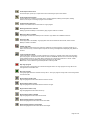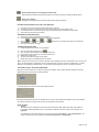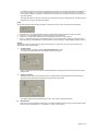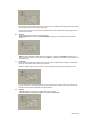
1
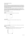
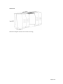
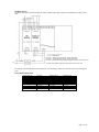
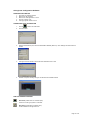
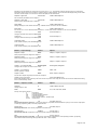
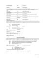
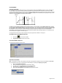
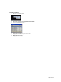
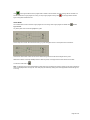
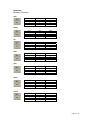
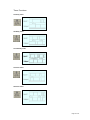
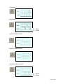
CALogix Programming and Installation Manual DM000M22 Page 1 of 44 Introduction Installation Mechanical Installation a) Base-unit b) Control module c) Mounting d) Removing a module e) Removing the base-unit from DIN-rail f) Cleaning g) Dimensions 4 4 4 4 5 5 5 6 Electrical Installation a) Output devices b) Supply Voltage c) Wiring a connector d) Replacing modules e) Inductive loads f) EN61010 g) EMC guidelines h) Supply and RS485 communications connections i) Input options (module) j) Output options (module) k) Example circuit l) Input sensor selection 7 7 7 7 7 7 7 8 9 9 9 10 10 Configuring CALogix a) CALogix network b) Multiple CALogix network c) CALogix-sw minimum PC requirements d) Installing CALogix-sw e) Running CALogix-sw f) Using CALogix-sw 11 11 11 12 12 12 13 Diagnostics 13 CALogix-sw configuration software 14 Starting CALogix-sw 14 Connecting to a controller 14 CALogix-sw toolbar 14 Base-unit setup 15 Configuring a PID module a) Settings menu b) Viewing Parameter settings c) Changing a setting value d) Initial settings e) Park Mode f) Setpoint adjustment g) Autotune h) Proportional cycle time i) Second and third setpoints j) Heat-Cool k) Recalibration l) Linear inputs 16 16 16 16 16 17 17 17 17 18 18 19 19 Page 2 of 44 m) Error messages n) PID module settings 20 20 Programmer a) Function overview b) Accessing the programmer interface c) Programmer interface d) Creating a program e) Program segment types f) Program properties g) Reading program data from a controller h) Creating an additional program i) Selecting a program j) Insert segments to a program k) Deleting segments l) Modifying a program m) Running Programs n) Stopping a program 25 25 25 25 25 26 28 28 29 29 29 29 29 29 30 Logic I/O module and Logic Programming a) Overview b) Logic I/O module settings c) Accessing logic programming d) The logic toolbar e) Placing a function block on desktop f) Arranging function blocks g) Linking function blocks h) Function blocks - selecting operation − Logic Boolean Timer Counter Comparator − Input − Output Physical Output Changing setpoint Manual power Autotune Event input Program i) Inverting Inputs j) Validating a logic program k) Writing a logic program to a controller l) Running and stopping a logic program m) Trace mode 31 31 31 31 31 33 33 33 33 33 33 34 34 34 35 35 35 35 35 36 36 36 36 37 37 37 38 Appendix Function Block Operation a) Boolean tables b) Timer charts 39 39 40 Technical Specification 43 Safety and Warranty Information 44 Page 3 of 44 CALogix Installation Instructions System Overview CALogix is a modular multi-loop PID controller with logic function capability. The controller consists of a DIN-rail mount base-unit that incorporates the power supply, RS485 communications ports and slots for up to 4 control modules. The control modules are available as PID or Logic I/O and can be selected then mounted into the base-unit as required for the application. Variations in PID control modules include temperature sensor and linear (0-50mV, 4-20mA, 0-5V & 0-10V) inputs with options for relay, ssd or analog (4-20mA, 0-5V & 0-10V) outputs. Logic I/O modules have user defined 0-5, 010, 0-24Vdc inputs with relay or ssd outputs. All wiring connectors to the base unit and control modules are plug-in to reduce installation and maintenance times. CALogix is configured using the Windows™ based CALogix-sw configuration tool which is provided with each base-unit. PID setup, input & output parameter settings, profile creation and writing logic function block diagrams can all be performed within the software utility. These settings can be read, modified and written to and from the controller and also saved on the PC as a file to be recalled at a later date when required. The program also provides information on current process value, set-points and output status which can be useful when commissioning the system. Mechanical Installation The controller is designed as two main components BASE-UNIT DIN rail mount device containing main CPU and connections for up to 4 control modules. CONTROL MODULE PID or Logic control modules can be mixed as required for the application and plugged in to base-unit. 1 base-unit and 1-4 control modules must be used for operation of product. A CALogix system can only be configured using CALogix-sw pc-based software. MOUNTING To mount a base unit with control modules proceed as follows: 1. 2. Affix 35mm type DIN rail securely to mounting surface, minimum length 140mm. The unit should be mounted vertically as shown. Attach carrier unit to DIN rail ensuring the spring release is at the bottom, facing downward. Page 4 of 44 3. Ensuring the input terminals are facing downwards, add the control modules to base unit. Press the top and bottom tabs on the module lightly and ensuring module is kept straight, push to locate in base unit (see diagram below). Press 4. Pre-wire connectors and plug into the appropriate modules (we suggest wire markers for identification) REMOVING A MODULE 1. 2. 3. 4. Isolate supply to CALogix and all module input and output connectors. Unplug connectors to module requiring removal. Press tabs as shown above to release module. Carefully pull the module away from base-unit ensuring tabs are free to remove. REMOVING BASE-UNIT FROM DIN-RAIL 1. Isolate supply to CALogix and all module input and output connectors. 2. Unplug connectors to base-unit and all modules. 3. Insert screwdriver into DIN-rail release block and apply pressure away from the controller, the base-unit can then be removed. REPLACING A CONTROL MODULE When replacing a control module follow the instructions above for removing and installing control modules. If a control module is being replaced with another that has the same part number, all parameter settings will be automatically transferred from the base unit to the new module on re-powering the system, no reconfiguration will be required. If a module is being replaced with a module that has a different part number, ensure that the system is re-wired accordingly and the module settings are modified to reflect the changes made, before running your system. Failure to do so may result in dangerous operation or damage to the system. If you are replacing logic modules with PID modules, it is important to turn off or delete any associated logic. CLEANING Wipe down with damp cloth (water only). Page 5 of 44 DIMENSIONS Note Ensure adequate clearance for connectors and wiring Page 6 of 44 Electrical Installation The system is designed to be installed in an enclosure which provides adequate protection against electrical shock. The enclosure should also be of a sufficient IP (NEMA) rating for protection against water and dust. CALogix should be mounted in an enclosure with minimum internal dimensions of 160 wide x 125 high x 85 mm deep. OUTPUT DEVICES Three types of output are available on an output module: relay, solid state relay drive (ssd) and analog. Output 1 may be any one of the three options, output 2 can be relay or ssd and output 3 is always relay. Any of these outputs can be assigned as SP1, SP2 and SP3 using the CALogix-sw software. Check the model number and output configuration before wiring the instrument and applying power. See section on output options for more details. 1. Solid state relay drive 12Vdc +10/-15% (nominal), 20mA To switch remote SSR 2. Miniature power relay 2A/250Vac resistive, Form A/SPST contacts 3. Analog Output (Isolated) - NOT AVAILABLE WITH LOGIC I/O MODULE Specify 4-20mA 500Ω max, ±0.1% fs typical 0-5Vdc 10mA (500Ω min). ±0.1% fs typical 0-10Vdc 10mA (1KΩ min). ±0.1% fs typical SUPPLY VOLTAGE 18-30Vdc, 8 watts ±10% fluctuation permitted WIRING A CONNECTOR Prepare the cable carefully, remove between 6 and 8mm insulation and ideally tin or terminate to avoid bridging. Prevent excessive cable strain. Maximum recommended wire size 32/0.2mm 1.0mm² (18 AWG) REPLACING MODULES Hot plugging of modules should not be carried out. To change a module always depower the base-unit. Once power is reapplied the carrier will reload the settings for that module and continue with the original module settings. Hotplugging can cause the carrier to fail and is potentially dangerous. INDUCTIVE LOADS To prolong relay contact life and suppress interference, it is recommended engineering practice to fit a snubber (0.1µF/100Ω) between relay output terminals. CAUTION Snubber leakage current can cause some electro-mechanical devices to be held ON. Check with manufacturers specification. EN61010 - 1 / UL61010C-1/ CSA22.2 No 1010 Compliance shall not be impaired when fitted to the final installation. Designed to offer a minimum of basic insulation only. The body responsible for the installation is to ensure suitable for measurement category II or III To avoid possible hazards, accessible conductive parts of the installation should be protectively earthed in accordance with EN61010 for Class 1 equipment. Output wiring should be within a protectively earthed cabinet. *Sensor sheaths should be bonded to protective earth or not be accessible Live parts should not be accessible without the use of a tool. Page 7 of 44 EMC GUIDELINES We make a number of general recommendations that can reduce the possibility of EMC problems. 1) It is important to suppress CALogix relay contacts, this will reduce switching interference and also prolongs life of the contacts. RC Networks fitted across the relay contacts are recommended for resistive and larger inductive loads, values such as 0.1μF capacitor in series with a 100Ω resistor. For small inductive loads, a suitable rated VDR is recommended. For small inductive dc loads, relays etc, a suitably rated diode fitted in parallel with the load is recommended. 2) 3) CALogix should be mounted into a metal cabinet which is properly earthed, good all round metal shielding is important. It should be borne in mind that the wiring of the installation can significantly reduce the efficiency of the instrumentation immunity. This is due to the ease with which high frequency RF can enter via unprotected incoming and outgoing cables. Earthed thermocouples or sensors with screened cable, should be earthed at the cabinet entry point. Any long cables entering the control cabinet should be protected at the point where they enter the cabinet, large diameter ferrite sleeves are an economical and effective method of reducing high frequency RF, looping the cables through ferrite sleeves a number of times will improve the efficiency of the filtering. Alternatively for mains cables, the fitting of a suitable mains filter can provide good results. Data or communications cables should be screened. If using Belden 8132 connect drain wire to PIN 5 of a shielded RJ45 connector. Ideally data and sensor cables should be routed separately from power cables and away from inverters or other high power/frequency devices. Page 8 of 44 SUPPLY AND RS485 COMMUNICATIONS CONNECTIONS (BASE-UNIT) INPUT OPTIONS (MODULE) 7P---0A000 7P---0A000 7P---0B000 = 4-20mA 7P---0C000 = 0-5V 7P---0D000 = 0-10V 7P---0A000 7L---0E000 OUTPUT OPTIONS (MODULE) 7P111----7L111----- 7PB11----- = 4-20mA 7PC11----- = 0-5V 7PD11----- = 0-10V 7P211----7L211----- 7P221----7L221----- 7PB21 = 4-20mA 7PC21 = 0-5V 7PD21 = 0-10V Page 9 of 44 EXAMPLE CIRCUIT The circuit below shows an example applicaion which includes a base-unit that has one PID module and one logic module fitted. FS1 Fuse = 1A time lag type to IEC127. CSA/UL rating 250V FS2 Fuse = 2A time lag type to IEC127. CSA/UL rating 250V FS3 Fuse = High rupture capacity (HRC). Suitable for maximum rated load current S1 switch = IEC/CSA/UL approved disconnection device must be used It is strongly recommended that the power supply zero volts and all logic module zero volts are common to prevent ground loops. INPUT SENSOR SELECTION Thermocouple type B E J K L N R S T Resistance Thermometer rtd 2/3 wire Description Pt-30% Rh/Pt-6%Rh Chromel/Con Iron/Constantan Chromel/Alumel Fe/Konst Nicrosil/NiSil Pt-13%Rh/Pt Pt10%Rh/Pt Copper/Con Pt100/RTD-2/3 Sensor Range (°C) 0 to1800°C* 0 to 600°C 0 to 800°C -50 to 1200°C 0 to 800°C -50 to 1200°C 0 to 1600°C 0 to 1600°C -200 to 250°C -200 to 800°C Sensor Range (°F) 32 to 3272°F* 32 to 1112°F 32 to 1472°F -58 to 2192°F 32 to 1472°F -58 to 2192°F 32 to 2192°F 32 to 2192°F -273 to 482°F -273 to 1472°F * Note : Type-B accuracy not specified below 100°C/212°F Page 10 of 44 Configuring CALogix CALogix is configured using Windows-based CALogix-sw software. Before using CALogix–sw, connect CALogix to a PC as shown below: CALOGIX NETWORK To other CALogix controllers RS232/485 converter RS485 from PC <1200m <15m CALogix uses RS485 full duplex serial communications link which is the standard most commonly used for industrial applications due to high noise immunity and multi-drop capability. It enables a PC to communicate with up to 31 CALogix base-units over distances up to 1200 metres, and requires the addition of an RS485 interface card, or a separate RS232 / 485 converter connected to the RS232 port of the PC. RS485 converters that derive power from the RS232 port must have all 9 pins (RS232) connected for full operation of the converter. RS485 cards and converters can differ greatly in their requirements and therefore the installation instructions supplied with the interface should be read carefully. 2m CALogix-PC cable (part number - CAB RJ45 2M 01) and a RS232/485 converter (part number 3C 25 000 K 3X) that fits directly on to the RS232 serial port on a PC are available from your nearest CAL Controls distributor. If wiring your own cable the RS485 connections are as follows. RJ45 PIN 2 3 4/5 6 7 RX+ RXGND TXTX+ As CALogix is designed for an industrial environment, CAL recommends using a 4 wire shielded RS485 cable such as Belden 8132. Ensure that connectors are suitable for use with shielded cable and are correctly bonded. Auto-baud rate function. On power up CALogix detects the network speed and automatically adjusts its baud rate accordingly. If the network baud rate is later modified, remove the power and reapply so that CALogix can resynchronise to the new baud rate. MULTIPLE CALOGIX NETWORKS Each CALogix unit has an RS485-in and RS485-out RJ45 socket. To connect a number of CALogix units on a network, wire as shown below. The cables should be wired so that the corresponding pins of RS485-out are connected to the same pin number on RS485-in of the next controller i.e. Pin 2 (out) to Pin 2 (in), Pin 3 (out) to Pin 3(in), Pin 5(out) to Pin 5(in), Pin 6(out) to Pin 6(in) and Pin 7(out) to Pin 7(in). Page 11 of 44 For multiple instrument networks each transmission line must be properly terminated to prevent reflections. 120Ω termination resistors should be fitted between TX+ & TX- and RX+ & RX- at the connection to the PC in addition to the last instrument in the chain. See example below. When transmission lines are not transmitting, they remain in an intermediate state which can allow receivers to receive invalid data bits due to electrical noise on the cable. To prevent this bias resistors may be required to force the lines into a known state. Some RS485 interface cards and converters may have bias resistors fitted please check manufacturer’s specification and recommendations for use of bias resistors. Note: The default Modbus address for each base-unit is 1, for a network with a number of CALogix units, power-up each unit individually and configure them with a unique Modbus address using CALogix-sw configuration tool. (See section on base-unit set-up in manual) CALOGIX-SW MINIMUM PC SYSTEM REQUIREMENTS As a general requirement, we would recommend a minimum of Pentium 450MHz with 256MB RAM, Windows and screen resolution, 1024 x 768. TM 2000/XP INSTALLING CALOGIX-SW 1. 2. 3. Insert CALogix-sw disk into CD-drive. CALogix-sw install program should auto-run. If this does not happen, manually run ‘setup.exe’ on CALogix-sw cd. Follow on screen instructions to complete installation. RUNNING CALOGIX-SW 1. 2. 3. Click ‘start’ on Windows toolbar. Mouse-over ‘all programs’. Mouse-over ‘CALogix folder’ in menu. Page 12 of 44 4. 5. Click on ‘CALogix’ icon. CALogix program should now run. USING CALOGIX-SW 1. Refer to on-screen help or CALogix programming manual contained on CALogix-sw CD. Diagnostics Each control module has LEDs to indicate when each of the outputs are on (or relay closed). If an analogue output option is fitted the LED dims proportionately with the output level, e.g. a PID module with a 4-20mA output, the LED will be dim at 4mA and bright at 20mA. Note: The output and the LED indicator are physically linked and always represent the true state of the output. CALogix base-unit has three status LED’s to assist with diagnosing problems LED 1 – Communications Off No communications On/Pulsing Communications active LED 2 – CALogix healthy (Heartbeat) Slow pulse Unit operating correctly Fast Pulse Base-unit emergency (comms still running) On Base-unit lock-up When base-unit emergency/lock-up conditions exist recycle power to clear. If the problem does not clear on power recycle contact CAL controls for technical support. LED 3 – Logic Off On Logic not active Logic active To start logic program running refer to section on running logic programs Page 13 of 44 CALogix-sw Configuration Software STARTING CALOGIX-SW 1. 2. 3. 4. 5. Click ‘start’ on Windows toolbar Mouse-over ‘all programs’ Mouse-over ‘CALogix folder’ in menu Click on ‘CALogix’ icon CALogix program should now run CONNECTING TO A CONTROLLER 1. Click on to add a new instrument 2. Click on browse 3. Select communications port, baud rate and Modbus address (default 1). Once settings are entered click on browse. 4. CALogix unit is then shown in device list when detected. Click on OK. . 5. Window now opens showing CALogix unit with data on installed modules THE CALOGIX-SW TOOLBAR New meter (visible when no controller open) Search for a CALogix system on a network. New device (visible when controller open) Access a different CALogix base-unit. Page 14 of 44 Open File Open controller application settings or logic program file. Note : when a saved application or logic file is loaded to a CALogix unit, the logic program will not be running. Save Save controller application settings or logic programs. Export Application Creates rich text file (.rtf) with application settings data Export device Creates rich text file (.rtf) with current device settings data Export program (only available when programmer interface is open) Creates rich text file (.rtf) with device program data Export logic (only available when logic desktop is open) Creates rich text file (.rtf) with logic program data Properties Select security settings, see section on security settings Edit programs Open programmer interface for profile creation, see section on programmer Edit logic Open logic desktop, see section on logic programming About BASE UNIT SETUP To access settings for a base unit 1. Right-click on controller image. 2. 3. Mouse over properties, then left-click on base-unit, see diagram above. Double-click on (+) to expand menus. 4. Base-unit settings are shown as below. Base-unit Configuration Default Options Baud rate 9600 2400, 4800, 9600, 19200, 38400, 57600, 115200. (read only) The network baud rate can be read. CALogix baud rate is automatically set on power-up to match the baud rate used by the Modbus master. Modbus address 1 1 to 255, step 1 The base-unit Modbus address can be set to a value of 1 to 255. A maximum of 31 base-units can be connected in a network. Base-unit diagnostics Default Serial number Preset (read only) The CALogix serial number is factory set before shipment Firmware version Preset (read only) Note : If the Modbus address is changed CALogix-sw will loose communications with the base-unit as it is still communicating using the original address. If the address is changed, exit CALogix-sw and browse for the controller using the new address. Page 15 of 44 CONFIGURING A PID MODULE SETTINGS MENU To access settings for a PID module 5. Right-click on controller image. 6. 7. Mouse over properties, then left-click on the required PID module number, see diagram above. The settings menu will now open VIEWING PARAMETER SETTINGS 1. CALogix PID module settings are split into various sub-menus to simplify finding the correct parameter These are − Module settings − Input settings − Output settings − Setpoint1 control − Autotune setting − Setpoint2 control − Setpoint3 control − Programmer 2. 3. 4. 5. For details of parameters in each of the sub-menus see section on ‘PID Module settings’. To expand a sub-menu double-click on ‘+’ next to the menu title. Scroll to find required parameter. To close sub-menu click on ‘-‘. CHANGING A SETTING VALUE 1. 2. 3. 4. 5. 6. Double-click on value box of parameter. Enter value for parameter. Some parameters will have a drop down list, select required option from list in these cases. Click on parameter name to accept setting. Repeat for all other required setting changes Once complete click on ‘apply’. The setting changes will now be written to controller. INITIAL SETTINGS There are a number of key settings required before initial operation of a CALogix PID module. 1. 2. 3. Input sensor type (Input settings menu) Select input sensor type from drop down list (Default J) When changing the sensor type ensure that the setpoint 1 upper and lower limits are set to values that will allow the setpoints you wish to enter If selecting linear refer to section on linear inputs Select operating unit (Module settings) Select process units from drop down list. Allocate outputs 1,2 & 3 (Output settings) Allocate physical outputs 1, 2 and 3 to SP1, SP2, SP3. Any physical output can be assigned as any setpoint, but each output can only be assigned once. Note: If the outputs have been previously allocated to a set-point and you wish to change assignment, then the outputs need to be set to none and this setting applied before you can re-allocate a new output to a setpoint. Please consider any wiring changes that may be required. Page 16 of 44 4. Once these settings have been made click on apply to write to the controller. PARK MODE Once initial settings are written to the controller it will still be in park mode i.e outputs to the controller are disabled. To take the controller out of park, change mode (setpoint 1 settings) to control type required i.e P (proportional), PI (proportional integral), PID (proportional integral derivative), PD (proportional derivative) or ON/OFF control. SETPOINT ADJUSTMENT Before carrying out an autotune or run with the default settings ensure the system is safe to operate at the setpoint value. To enter or adjust a setpoint 1: 1. Right click on controller image. 2. 3. Mouse-over properties and select programmer and set-points. Expand (+) setpoints menu. 4. Enter Setpoint 1 value for the required module (click out of value box once setting entered to ensure value is accepted) Apply setting and click OK New setpoint is now written to the controller and should be visible on controller image. 5. 6. Changes in setpoint 2 and 3 are made in the settings menu see PID module settings AUTOTUNE This is a single shot procedure to match the PID module to the process. Select either tune or tune-at-setpoint in the mode parameter of autotune settings for a specified module. The criteria for choosing the best autotune mode for an application is given below. The tune-at-setpoint program is recommended when: The process is already at setpoint and control is poor. The setpoint is less than 100°C in a temperature application Re-tuning after a large setpoint change. Tuning multi-zone and/or heat-cool applications. Notes: DAC is not re-adjusted by tune-at-setpoint. Before running autotune select whether autotune calculated proportional cycle time is to be used see below. The tune program should be used for applications other than those listed for tune-at-setpoint shown above. As autotune is running, tune or atsp is displayed on the CALogix module image within CALogix-sw. Once tuning is complete, the message will no longer be visible. PROPORTIONAL CYCLE-TIME The choice of cycle-time is influenced by the external switching device or load. eg. contactor, SSR, valve. A setting that is too long for the process will cause oscillation and a setting that is too short will cause unnecessary wear to an electromechanical switching device. To select AUTOTUNE calculated CYCLE-TIME − In ‘autotune settings’ menu for chosen module, change autotune cycle-time parameter to yes. If the autotune cycle-time is not required, set parameter as no and cycle time parameter value in setpoint settings will be used. (default value 10S) Page 17 of 44 Cycle time recommendations − It is recommended that relay outputs should not have a cycle time of less than 10S. If a cycle time of less than 10s is required, solid state drive outputs are advised. SECOND AND THIRD SETPOINTS (SP2 and SP3) Primary Alarm Modes − Configure SP2 and SP3 outputs to operate as an alarm from setpoint 2 and 3 control sections in the ‘module settings menu’ The alarms will be individually triggered when the process value changes according to the options listed below. DVHI Rises above the main setpoint by the value inserted at setpoint 2 or 3 DVLO Falls below the main setpoint by the value inserted at setpoint 2 or 3 Band Rises above or falls below the main setpoint by the value inserted at setpoint 2 or 3 FSHI Rises above the full scale setting of setpoint 2 or 3 FSLO Falls below the full scale setting of setpoint 2 or 3 COOL Heat-cool operation, see section on heat-cool EOP Event Output (See Programmer section) Subsidiary SP2 / SP3 modes − The following additional subsidiary alarm functions can be added to any primary alarm configurations. − Latch Once activated, the alarms will latch and can be manually reset via CALogix-sw or an operator panel when the alarm condition has been removed. Hold This feature inhibits alarm operations on power-up and is automatically disabled once the process reaches the alarm setting. Lt.ho Combines the effects of both Latch and Hold and can be applied to any primary alarm configuration If you configure SP2 or SP3 as an alarm in on.off mode please be aware the output and LED indicator to the alarm will be energised when the alarm is not active and de-energised when alarm is active. By setting display alarm (setpoint 2 and 3 settings) to on the alarm display indicator (bell) will replace the output LED in CALogix-sw when an alarm condition exists. Note : Changing SP2 or 3 operating mode will default the setpoint back to zero when applied to the base-unit, this will not be updated in the property sheet until closed and read back. HEAT-COOL Heat-cool strategy is a feature that improves control of processes that need heating and cooling, for example: − − Environmental test chambers used in rooms where ambient temperature can vary above and below test temperature. Plastics extruders where the material initially needs heating, then cooling, when it begins to heat itself exothermically due to pressure and friction applied by the process. The purpose of cool strategy is to maintain accurate control of the process with a smooth transition between heating to cooling. This is achieved by using PID control for both heating and cooling with the proportioning bands linked by an adjustable deadband. Tuning CALogix for heat-cool Enter a setpoint then allow the process to reach the setpoint using factory settings for heating only. Ensure that procedure for initial settings has been carried out before heating the application. When application process value has stabilised at setpoint change the following parameters Parameter Menu Value DAC Setpoint 1 control 1 Cycle time Setpoint 1 control 10 COOL Operating mode Setpoint 2 control Cycle time Setpoint 2 control 10 Use cycle time Autotune settings No Apply these settings then set Mode Autotune settings ATSP When the setting is applied there will be a temporary disturbance in temperature as autotune is running. ‘ATSP’ is displayed on the module within CALogix-sw controller image. Once ‘ATSP’ is no longer displayed the controller is tuned. Further settings If regular oscillations occur change Use cycle time to Yes. See section on proportional cycle time. Note : minimum recommended cycle time using relay outputs is 10s. Page 18 of 44 Autotune sets PID terms for Heat and Cool with the same setting values. Band, integral time, derivative time, DAC and derivative sensitivity settings can all be modified independently for both heat (setpoint 1 settings) and cool (setpoint 2 settings). In some processes oscillations occur during cooling. If this occurs double the value of band (setpoint 2 settings). If no improvement return band (SP2) to its original value and half the cycle time (setpoint 2 settings) If the process hunts between heating and cooling a deadband setting may be needed. Enter a small value e.g.1 for Setpoint 2 (setpoint 2 settings) Water cooled applications Water cooled applications at temperatures greater than 100°C may suffer from the non linear effect caused by water turning to steam. This can be countered by setting subsidiary mode (setpoint 2 settings) to NLIN. Multi zone applications When tuning multi zone applications like extruders, distortions due to thermal interaction between adjacent zones can be minimised by running autotune on all controllers at the same time. RECALIBRATION F If the controller and instrument readings are different, the zero and span (input settings) will require adjustment. Adjust zero to make an equal adjustment across the full scale of the controller and/or span to make a correction where the error increases or decreases across the scale. 1. To adjust the zero function substitute the measured values in the expression Instrument reading − controller reading = zero Example: Instrument reading = 245 Controller reading = 250 245 − 250 = −5 Adjust zero to -5 to correct the error. 2. Adjusting the span function i.e. to make a correction when errors are different across the scale. a) Choose a temperature near the bottom and another near the top of the scale b) Run the process at the lower temperature (T1). Note the error (E1) between the controller and the instrument readings. c) Check value of setpoint 1 upper limit (SP1UL) in input settings menu. d) Repeat at the upper temperature (T2) and note error (E2) e) Substitute the values for T1, T2, E1, E2 in the expression below; E2 − E1 X SP1UL = span T2 − T1 Example Instrument reading Controller reading Error T1 58 60 E1= −2 T2 385 400 E2 = −15 . Substituting values in the formula (−15) − (−2) x 450 = (−13) x 450 = −17.9 385 − 58 327 Therefore adjust span to −18 to correct error. Notes: 1. After making the adjustment the reading will immediately change. Allow time for the temperature to stabalise at T2 before making any further adjustment. At this point zero adjustment may be needed, refer to step 1 above. 2. Check that the temperature correctly stabalises at T2 and then adjust setpoints to T1. If an error is present at T1 repeat from step 2. LINEAR INPUT Modules can be ordered with analog inputs for use with other field devices and instruments. Check the specification of the device providing the input to ensure it is compatible. Set-up Procedure − 4-20mA The 4–20mA input model converts current into voltage using an internal resistor which spreads the signal across the input range 10 to 50 mV using a multiplier of 2.5. When using a transducer with an output less than 4–20mA, the input maximum and minimum mV values can be calculated using the same multiplication factor. Page 19 of 44 − 0-5V Models with 0 to 5V input use an internal resistor to spread the signal across the input range 0 to 50 mV using a divider of 100. Where a transducer provides a smaller output, the input maximum and minimum values can be similarly calculated. − 0-10V Models with 0 to 10V input use an internal resistor to spread the signal across the input range 0 to 50 mV using a divider of 200. Where a transducer provides a smaller output, the input maximum and minimum values can be similarly calculated. Decide what scale minimum and maximum will be required, and whether the scale needs inverting. Example The example below gives an example of how a 4–20mA input could be configured for an application. The input to the controller is linear where 4mA = 80 units and 20mA = 300 units. Action Parameter Menu Parameter Value Select input sensor type Input settings linear Select unit Module settings select from list, if unit not available select Set Allocate SP1 output Output settings Select output 1, 2 or 3 Enter Linear high Input settings Enter 50 (represents 20mA i.e. multiplier 2.5) Enter Linear low Input settings Enter 10 (represents 4mA i.e multipler 2.5) Enter Linear low scale Input settings Enter 80 (i.e. units at 4mA) Enter Linear high scale Input settings Enter 300 (i.e. units at 20mA) Enter display resolution Input settings Set as 0.01, 0.1, 1 Note: changing the display resolution will affect set-point value and other operating parameters. Ensure that display resolution settings are selected before adjusting set-point and tuning the controller to the application. ERROR MESSAGES CALogix-sw error messages are shown below Tune Fail - Will be displayed if an autotune cycle fails 1. 2. Check setpoint is not set at 0 The characteristics of the load exceed the algorithm limits i. Change conditions e.g. raise setpoint ii. Try tune at setpoint, atsp iii. If error persists call local CAL representative. Input Fail – Sensor is open/short circuit or linear input is over range. Check sensor/wiring/connections. Error On/Off – Error On/Off will be displayed if autotune when in On/Off control. PID MODULE SETTINGS (* = module position number) Module * - settings Default Options Module name Module * User defined A user defined label (name) up to 10 characters can be set for each module. Operating units None °C, °F, Bar, PSI, PH, RH, Set, None Process-value operating units can be defined as °C, °F, Bar, PSI, Ph, RH or Set. Important note: If switching from °C to °F or vice versa, ensure that set-point and other temperature-value based parameter settings are adjusted accordingly to reflect the change made. Failure do so may result in dangerous operation or damage to the system. Module * – input settings Default Options Sensor Type J Display Resolution 1 B, E, J, K, L, N, R, S, T, RTD 2-wire, RTD 3-wire, linear, custom sensor**, custom sensor with cjc**. **consult factory 0.01, 0.1, 1 Page 20 of 44 Resolution of PV and Setpoint on CALogix-sw can be set as 0.01, 0.1 or 1. This resolution is also the format used for the corresponding data register with CALogix unit to be read by an operator panel or for data acquisition. It is recommended that display setting of 0.01 is NOT used when a thermocouple or PT100 sensor is used as the displayed value will fluctuate. Setpoint 1 upper limit Sensor Max -9999 to 9999 step 0.01 Sets a maximum permissible value for Setpoint 1 Setpoint 1 Lower limit Sensor Min -9999 to 9999 step 0.01 Seets a minimum permissible value for Setpoint 1 Span Offset 0.0 -9999 to 9999 step 0.01 Realigns readings to match another instrument e.g. calibration source or meter see note on recalibration. Zero offset 0.0 -9999 to 9999 step 0.01 Zero sensor error. +ve zero offset increases measured PV, -ve zero offset reduces measured PV, see note on recalibration. Linear High 50.0 0.0 to 50.0 step 0.1 Configures maximum linear input see Linear inputs Linear Low 10.0 0.0 to 50.0 step 0.1 Configures minimum linear input, see Linear inputs Linear high scale 1000 -9999 to 9999 step 0.01 Scale controller to display value at Linear high value Linear low scale 0 -9999 to 9999 step 0.01 Scale controller to display value at Linear low value Module * - Output settings Default Options Setpoint 1 output None Output 1, Output 2, Output 3 Select physical output to be assigned as Setpoint 1. Setpoint 2 output None Output 1, Output 2, Output 3 Select physical output to be assigned as Setpoint 2 Setpoint 3 output None Output 1, Output 2, Output 3 Select physical output to be assigned as Setpoint 3 Output 1, 2 & 3 burnout state De-energised De-energised, Energised Configure state of outputs on sensor burnout / break Output 1, 2 & 3 inversion False False, True None None, Output 2, Output 3 Reverse operation of outputs Output 1 inhibit Prevents other outputs energising at the same time as Output1 Output 1,2 & 3 cycle count - Count value (Read only) Each module internally stores a read-only value of the number of cycles for each output, this can be used to check the estimated remaining life of a mechanical relay, if fitted. Module * – Setpoint 1 control Default Options Setpoint 1 0 -9999 to 9999, step 0.01 Park P, PI, PID, PD, Park, On/Off Change setpoint 1 value Mode Primary control type for setpoint 1 P PI PID PD Park On/Off Band Proportional Proportional Integral Proportional Integral Derivative Proportional Derivative Holds controller operation – disables output On/Off Control 10 0 to 9999, step 0.01 SP1 proportional band or Hysteresis -* 100% sensor maximum, proportional control eliminates the cycling of on-off control. Output power is varied, by proportioning action, across the proportional band Integral Time 5 mins 0 to 9999, step 0.1 SP1 integral time/reset - Auto-corrects proportional control offset error Derivative time 25 secs 0 to 200, step 1 SP1 derivative time/rate - Suppresses overshoot and speeds response to disturbances DAC 2 0.5 to 8, step 0.5 SP1 derivative approach control dAC - Tunes warm-up characteristics, independent of normal operating conditions, by adjusting when derivative action starts during start-up (smaller dAC value = nearer setpoint). Page 21 of 44 Derivative Sensitivity 0.5 0-1.5, step 0.1 Cycle time 10 secs 0.1 to 9.9, step 0.1 10 to 81, step 1 SP1 proportional cycle-time - Determines the cycle rate of the output device for proportional control. The choice of cycle-time is influenced by the external switching device or load. eg. contactor, SSR, valve. A setting that is too long for the process will cause oscillation and a setting that is too short will cause unnecessary wear to an electro-mechanical switching device. Control offset 0 -9999 to 9999, step 0.01 SP1 offset/manual reset - * ±50% band. Applicable in proportional and ON/OFF mode with integral disable: Integral time = OFF. Maximum power 100 0 to 100, step 1% Maximum % proportional output of SP1. When using proportional control the output of SP1 will not exceed maximum power setting. Minimum power 0 0 to 100, step 1% Minimum proportional output of SP1. When proportional control is used the output of SP1 will not reduce below the minimum power setting. Output power Read Only 0 to 100, Step 1% The current proportional output of SP1 shown as %. Manual Power Off Off, 0 to 100, step 1% Manual power overrides PID calculated power output. The proportional output for SP1 will remain constant at the entered value. To return to PID control set manual power to 0. Module * – Autotune Settings Default Options Mode Off Off, tune, atsp Off Tune ATSP Run current PID or On/Off settings Tune controller at 75% of set-point Tune controller at setpoint Use cycle time No Yes No No, Yes Use manually entered cycle time Automatically apply autotune calculated cycle time Band Read Only Autotune calculated proportional band Integral time Read Only Autotune calculated Integral time DAC Read Only Autotune calculated derivative approach control Cycle time Read Only Autotune calculated cycle time CtA, CtB, Ct1, Ct2, Ct3, Ct4, Os1, Os2, Us Read Only, Autotune data Module * - Setpoint 2 Control Default Options Operating mode None DVHI, DVLO, BAND, FSHI, FSLO, COOL, EOP, None DVHI DVLO Band FSHI FSLO Cool EOP Mode Deviation high, alarm output if process value rises above the main setpoint by the value inserted at setpoint2 Deviation low, alarm output if process value falls below the main setpoint by the value inserted at setpoint 2 Band, alarm output if process value rises above or falls below main setpoint by value inserted at setpoint2 Full scale high, alarm output if process value rises above the value inserted at setpoint2 Full scale low, alarm output if process value falls below the value inserted at setpoint2 See section on heat-cool See event outputs in programmer section PARK P, PI, PID,PD, PARK, On/Off Primary control type for setpoint 2 P Proportional PI Proportional Integral PID Proportional Integral Derivative PD Proportional Derivative Park Holds controller operation – disables output On/Off On/Off Control PI, PID and PD can only be selected when operating mode is set as Cool Subsidiary mode None LTCH, HOLD, LTHO, NLIN Setpoint 2 0 -9999 to 9999 step 0.01 Page 22 of 44 Change setpoint 2 value Band 2 -9999 to 9999 step 0.01 SP2 proportional band or Hysteresis -* 100% sensor maximum, proportional control eliminates the cycling of on-off control. Output power is varied, by proportioning action, across the proportional band Integral time 5 mins 0 to 1000, step 0.1 SP2 integral time/reset - Auto-corrects proportional control offset error Derivative time 25 secs 0 to 200. step 1 SP2 derivative time/rate - Suppresses overshoot and speeds response to disturbances DAC 2 0 to 5 step 0.5 SP2 derivative approach control dAC - Tunes warm-up characteristics, independent of normal operating conditions, by adjusting when derivative action starts during start-up (smaller dAC value = nearer setpoint). Derivative sensitivity 0.5 0.1 to 1, step 0.1 Cycle time 10 secs 0.1 to 9.9, step 0.1 10 to 81, step 1 SP2 proportional cycle-time - Determines the cycle rate of the output device for proportional control. The choice of cycle-time is influenced by the external switching device or load. eg. contactor, SSR, valve. A setting that is too long for the process will cause oscillation and a setting that is too short will cause unnecessary wear to an electro-mechanical switching device. Maximum power 100 0 to 100, step 1 Maximum % proportional output of SP2. When using proportional control the output of SP3 will not exceed maximum power setting. Minimum Power 0 0 to 100, step 1 Minimum proportional output of SP2. When proportional control is used the output of SP3 will not reduce below the minimum power setting. Output power Read Only 0 to 100, step 1 The current proportional output of SP2 shown as %. Manual power Off Off, 0 to 100, step 1 Manual power overrides PID calculated power output. The proportional output for SP1 will remain constant at the entered value. To return to PID control set manual power to 0. Display alarm No No, Yes When set to yes, alarm symbol is shown on controller image within CALogix-sw when an alarm output is switched. Reset latched alarm No No, Yes Used to clear a latched alarm output on SP2, once the alarm condition has cleared. Set value to yes to clear. Module * - Setpoint 3 control Default Options Operating mode None DVHI, DVLO, BAND, FSHI, FSLO, EOP, None Mode Primary control type for setpoint 3 PARK P, PARK, On/Off P Park On/Off Proportional Holds controller operation On/Off Control Subsidiary mode None LTCH, HOLD, LTHO Setpoint 3 0 -9999 to 9999, step 0.01 2 -9999 to 9999, step 0.01 Change setpoint 3 value Band SP3 proportional band or Hysteresis -* 100% sensor maximum, proportional control eliminates the cycling of on-off control. Output power is varied, by proportioning action, across the proportional band Cycle time 10 0.1 to 9.9, step 0.1 10 to 81, step 1 SP3 proportional cycle-time - Determines the cycle rate of the output device for proportional control. The choice of cycle-time is influenced by the external switching device or load. eg. contactor, SSR, valve. A setting that is too long for the process will cause oscillation and a setting that is too short will cause unnecessary wear to an electro-mechanical switching device. Maximum power 100 0 to 100, step 1 Maximum % proportional output of SP3. When using proportional control the output of SP3 will not exceed maximum power setting. Minimum Power 0 0 to 100, step 1 Minimum proportional output of SP3. When proportional control is used the output of SP3 will not reduce below the minimum power setting. Output Power Read Only 0 to 100, step 1 Page 23 of 44 The current proportional output of SP3 shown as %. Manual Power Off Off, 0 to 100, step 1 Manual power overrides PID calculated power output. The proportional output for SP3 will remain constant at the entered value. To return to PID control set manual power to 0. Display Alarm No No, Yes When set to yes, alarm symbol is shown on controller image within CALogix-sw when an alarm output is switched. Reset Latched Alarm No No, Yes Used to clear a latched alarm output on SP3, once the alarm condition has cleared. Set value to yes to clear. Module * - Programmer Default Options Program number 0 1 to 31 Select programmer profile to run. See section on programmer Run mode Off Hold, Run, Off Program run mode. See section on programmer Page 24 of 44 PROGRAMMER FUNCTION OVERVIEW The Programmer function enables CALogix to control applications that require setpoint changes over time. Examples of this are ramp changes where setpoint is gradually increased at a specified rate until a target level is reached or step changes which are instantaneous. These can be separated by soak periods during which the process is held at a constant value. Each individual time interval of the program or segment, together with it’s associated moving setpoint value can be stored as a unique program. An example is shown below. Setpoint Step Soak Ramp Time (segments) In addition to those settings that determine the segment profile, it is also necessary to set program start values, together with the preferred ramp rate time units for each individual program. At the end of a sequence, a program can be arranged to repeat (loop), either a specified number of cycles, or continuously. Only one loop can be included in a program. When the program is running, CALogix-sw indicates progress through the sequence of segments and can additionally be interrogated for further segment information. It is also possible to Call an already existing program as a sub program that can be inserted as a segment of another program. The programmer functions can be fully configured using the programmer interface in CALogix-sw. ACCESSING THE PROGRAMMER INTERFACE 1. Click on the icon in the main toolbar. 2. Programmer interface should now be open . THE PROGRAMMER INTERFACE The programmer interface is shown below. CREATING A PROGRAM. Note : If a program is running in any module on the carrier the programmer interface will only be available in view mode only. All programs have to be in an OFF state to enable editing of a profile.(see stopping a program) 1. 2. 3. 4. 5. Open the programmer interface. Select module tab corresponding to required PID module. On toolbar click on programmer menu select new program. When pointer is in profile chart area right click mouse. Mouse over add segment and the following menu should be shown. Page 25 of 44 6. 7. To add segments click on ramp/soak/step. Enter quantity of segments required then press OK. 8. 9. Click and drag segment points on the profile chart area to draw the required profile. Click to open data for each segment in segment property menu. 10. Adjust values for any parameters that require modification. (see section on segment parameters). 11. If you require to add additional segments (ramp/soak/step), call programs, event inputs, event outputs or loops, see notes below. 12. Once the profile is created click on programmer menu then click on write program data. 13. The program is now written to the controller. PROGRAM SEGMENT TYPES Ramps During a ramp segment the setpoint will change at a user defined rate until a target setpoint is reached. The ramp rate entered is set as process units per hour or minute, refer to section on program properties to configure. If the ramp rate is set too high, setpoint may become much higher (or lower, if cooling) than process value. In this case, the holdback band function will hold the moving setpoint when the process value falls out-with the number of units set in the holdback band. Once the process value increases to fall within the band value, the moving setpoint will resume ramping at the specified rate. Soaks During a soak cycle the setpoint will be held constant for a user defined period of time. Click soak time parameter value box and time is displayed as hh:mm:ss. Enter soak time required then click on parameter name, the soak time displayed is then displayed as total number of seconds. At the end of the soak period an event output can be triggered see notes on Event outputs below. Step A step is an instantaneous change in setpoint. Please note that it can take a process value some time to reach target setpoint after a step function. If a soak function is preceded by a step function, the soak period commences immediately after the setpoint has changed and not when the process value reaches setpoint, this can result in the soak period appearing to be shorter than expected. At the end of the soak period an event output can be triggered, see notes on Event outputs below. Event outputs SP2 and SP3 output state can be changed at various points of the program using event outputs. Page 26 of 44 Event outputs can be selected as an individual segment or after other segment types have completed such as ramps, soaks, steps and loop. Outputs must be assigned as event outputs in setpoint 2 and/or setpoint 3 control settings menu before EOP’s can be used. See section on PID Module settings. Once outputs are configured select the correct EOP status for program segment. None 2D 2E 3D 2E 2D 3D 2E 3D 2E 3E 2D 3E No event output. SP2 output de-energised to mark event. SP2 output energised to mark event. SP3 output de-energised to mark event. SP3 output energised to mark event. Both SP2 and SP3 outputs de-energised to mark event. SP2 output energised and SP3 output de-energised to mark the event. Both SP2 and SP3 outputs energised to mark event. SP2 output de-energised and SP3 output energised to mark the event. Note: Only valid options will be displayed on the menu for selection. If required option is not shown ensure that SP2 and SP3 outputs are configured correctly. Event outputs are a change of state of SP2 or/and SP3. This state will remain until another event output is used to reverse it or the program is stopped. Event inputs When an event input is used, a program is held at that point until a signal to proceed is received via a logic program. When the program is held awaiting an event input, the temperature (or other process value) is held constant until the input is received. The event input number should be selected to match the event input in the logic program. Call If the same profile is required as part of a number of programs, it can be saved as a program and called into another program when required. By inserting a call segment and choosing the required program the profile section will be added. This will be shown on the profile chart as a shaded section. Called program Loop The loop function will run the same profile a specified number of times (recycle count). E.g. If a program has a recycle count of 5 the profile will run 6 times in total. Only one loop can be used in a program. Once the number of loops are completed an event output can be triggered, see notes on Event outputs. Page 27 of 44 PROGRAM PROPERTIES Program properties allows you to set parameters for a program displayed on the profile chart area. When a program is displayed on the user interface click on properties in the programmer menu. The program properties box should now open Current program tab Program Number Displays the number of the currently open program. Description A user defined label (name) can be set as a program name. Power Fail After a power failure one of three options can be chosen. Continue – Resume program from last point before failure. Hold – Hold program at current point until manually restarted. Reset – Restart program from beginning. Ramp rate units Set ramp rate units as minutes or hours. Program start point Start program from process value or set-point. Colours Tab The grid, main program profile, sub program profile, background, loop marker, EOP marker and EIP marker colours can be set for the profile chart area. Scales Tab Scale maximum and Scale minimum settings can be set for profile chart area. By selecting full screen on scale display mode the profile scales are resized to fit on screen. READING PROGRAM DATA FROM A CONTROLLER (Note that program data is read from the controller when opening the programmer interface. The read program data function is used to recover program data that has been modified in the programmer interface but not written to the controller. 1. When the programmer interface is open click on required module tab. Page 28 of 44 2. 3. Click on read program data in the programmer menu. Information from the controller is read and program 1 is displayed on the programmer interface. CREATING AN ADDITIONAL PROGRAM 1. Follow instructions in section on creating a program. SELECTING A PROGRAM 1. When the programmer interface is open click on the required module tab. 2. Click on select program in the programmer menu. 3. Select required program. 4. The selected program will now be displayed on the program interface. INSERT SEGMENTS TO A PROGRAM 1. When the programmer interface is open click on required module tab. 2. Select program required in the programmer menu. 3. In the profile chart click to highlight segment point where the additional segments are to be inserted. 4. Right click the mouse in profile chart area. 5. Mouse over insert segment then click on ramp/soak/step. 6. Select the number of segments to insert. 7. Adjust segments to create profile as required. see creating a program. 8. Write program data in programmer menu. DELETING SEGMENTS 1. In the profile chart, click to highlight the segment node that requires deletion. 2. Right click in the profile chart area. 3. Click on delete segment. 4. Click OK to accept segment delete. 5. The segment is now deleted from the program. MODIFYING A PROGRAM 1. Open the programmer interface and select the tab for required module. 2. Select the program to be modified, see Selecting a program. 3. Click and drag chart points to create required profile. 4. Write program data in programmer menu. RUNNING PROGRAMS 1. 2. Ensure that programs are written to the controller and programmer interface is closed. Right click on controller image. 3. 4. 5. Mouse-over properties and select programmer and set-points. Expand (+) programmer menu. 6. 7. 8. 9. 10. Scroll to required module. Enter program number to be run i.e. Module * - Program Number. Set program run mode to on. Apply settings to controller. The selected program will now run. Page 29 of 44 STOPPING A PROGRAM 1. Right click on controller image. 2. 3. Mouse over properties select programmer and set-points. Expand (+) programmer menu. 4. 5. 6. 7. Scroll to required module. Set program run mode of required module to off. Apply settings to controller. The program will now stop. Page 30 of 44 Logic I/O Module and Logic Programming OVERVIEW CALogix has integrated logic function capability that can be used for controlling a system by linking associated inputs and outputs using logic, timer, counter and comparator functions. A logic programming utility is included within CALogix-sw that can be used to create logic function block diagrams when a CALogix system has logic I/O modules fitted. The logic programming memory will allow programs up to 40 Boolean blocks or up to 16 timers/counters depending on the complexity of the blocks used i.e. some function blocks (e.g. timers) have been developed by using several other function blocks and will therefore require more memory. LOGIC I/O MODULE SETTINGS To access logic I/O settings right mouse click on the controller image, mouse over properties then click on the module number (module slot number must have logic I/O module fitted) The settings window will now open. A user-defined label (name) for the module can be entered in the module name field, once a label is entered click on the apply button to write the label to the controller. This label will be visible on the controller image in CALogix-sw and will be included when the application is exported to .rtf files. The label can have a maximum of 10 characters Input 1,2,3 range The voltage range of inputs 1, 2 and 3 can be user-defined as one of three voltage ranges i.e. 0-24V, 0-10V and 0-5V. These voltages are used to determine high and low states for logic functions and also for comparator switching levels. Voltages above 66% of the input range will be considered as high state and below 33% as low state e.g. for a 0-10V input range <3.3V = low logic state (0) and >6.6V = high logic state (1). Comparators will convert the input level to a percentage of full scale and will be compared against other inputs or a constant. e.g. With an input range of 0 - 24V, an input voltage of 2.4V will be considered to have a value of 10.0 in a comparator block. Each of the inputs can be independently set for a different voltage level input. Once each input has been set, write the settings to the controller by clicking the apply button. LOGIC PROGRAMMING CREATING LOGIC PROGRAMS ACCESSING LOGIC PROGRAMMING 1) 2) Click icon on main toolbar Logic programming desktop should now open THE LOGIC TOOL BAR Create Boolean function block AND, OR, XOR, LATCH, NAND, NOR, XNOR boolean function block can be created See section on Boolean function blocks. Create comparator function block Compare two I/O module inputs or compare an I/O block input with a constant. ‘greater than’ or ‘less than’ comparator options. See section on comparator blocks. Create timer/counter function block Select one of eleven timer types or two counter types. See timers/counters overview section. Page 31 of 44 Create input function block I/O module inputs, power up or output status can be used as logic input function blocks. Create output function block Function blocks for a switching a physical output, changing setpoint, selecting manual power, starting autotune, event input and running a program can be created. Function block linking tool Creates a link between two function blocks in a logic program. Read logic data from controller Existing logic data in desktop is overwritten by logic program read from controller. Write logic data to controller Logic program is written from desktop to the controller. Logic data is also validated at this time. Clear logic data Clears logic data on the desktop. Logic programs within the controller are NOT cleared, unless a blank desktop is written to controller. Validate logic data Logic validation ensures that a logic program is created as a functional program. If function blocks are not used in the correct way or links to inputs or outputs are missing a message will be displayed giving details of the error. Logic program trace mode Trace mode allows monitoring of a logic program that is running in a controller. Green lines show the active part of the program. Counter and timer values can also be read. Note: Windows is not a real-time operating system therefore there may be a delay before changes in the controller are visible on PC screen. If other applications are running in addition to CALogix-sw the delay may be greater. Note: When in trace mode the logic desktop will be in read-only mode. Stop logic program The logic program running within the controller are stopped. Note. The ‘logic program running’ LED on the CALogix base unit will switch OFF. Run logic program The logic program within the controller memory will run. The ‘logic program running’ LED on the CALogix base unit will switch ON. Align function blocks to left Align all highlighted function blocks with the blocks to the left. Align function blocks to right Align all highlighted function blocks with the blocks to the right Align function blocks to top Align all highlighted function blocks to the top. Align function blocks to bottom Align all highlighted function blocks to the bottom. Resize function blocks to same width Resize all highlighted function blocks to the same width. Resize function blocks to same height Resize all highlighted function blocks to the same height . Page 32 of 44 Resize function blocks to same height and same width Resize all function blocks to the height and width of the blocks to that of the widest and highest blocks. Apply grid to desktop Apply grid to the logic desktop to assist with aligning and creating programs. PLACING A FUNCTION BLOCK ON THE LOGIC DESKTOP 1) 2) 3) 4) Left-Click on the icon for the logic function block type you require. Continuing to hold the mouse button, drag the mouse pointer into the logic desktop area. Once mouse pointer is in position that you want to place function block, release the mouse button. The function block should now be visible. ARRANGING FUNCTION BLOCKS 1) Click’n’drag an area encapsulating function blocks 2) Function blocks that require rearranging should now be highlighted 3) 4) (left), (right) , Click on direction. The function blocks will now align. (up) or (down) icons to arrange function blocks in the required LINKING FUNCTION BLOCKS 1) Create required function blocks on logic desktop. 2) 3) 4) 5) 6) 7) Click on function block linking tool icon . Click and hold left mouse button in the centre of first block . Drag mouse pointer to the centre of second function block. Release left mouse button. The two function blocks should now be linked. Repeat from step 2 to link additional function blocks. Note: All timers have one input, but counters, Boolean and comparators have two. Output blocks have one input. All timers, counters, Boolean, comparators can have multiple outputs. Inputs can connect to multiple timers, counters, Boolean and comparators simultaneously. You cannot link physical outputs to inputs, use Output (In) blocks. FUNCTION BLOCKS - SELECTING OPERATION Each type of function block has a number of variations in operation. Once a block has been dropped on the logic desktop right click on the block and select properties. A window will open up with the function block settings window By clicking on the drop down menu for operation type (or mode in some blocks) the operation type can be selected. The various function block options and how they are configured is shown below. LOGIC BLOCKS I. Boolean Operation mode for a Boolean function block ban be selected as AND, NAND, OR, NOR, XOR, XNOR or LATCH (see selecting operation above.). Truth table for Boolean functions are given in truth tables in the appendix. Each Boolean function block requires a two inputs from either an input block or other function blocks. The output of the block must be connected to another function block or an output block. Page 33 of 44 II. Timers A number of timer functions are available with CALogix, these are: on-delay, off-delay, on-off delay, on-pulse, off-pulse, on-off pulse, delayed-pulse, symmetrical recycler pause, symmetrical recycler pulse, asymmetrical recycler pause and asymmetrical recycler-pulse. Timer charts showing the operation of these are shown in appendix The time settings are entered by clicking on the time required and entering the data in HHH.MM.SS.S format. Once entered click on OK to accept the settings change. All timers require a single input from either an input block or another function block. The block output must be connected to another function block or an output block. Time settings for standard timer types are set via CALogix software. To adjust timer settings remotely via an operator panel, SCADA or field device ensure that the ‘remote’ box is ticked in the function block ‘properties’. This feature is only available for ‘on’ and ‘off’ delay timers, other timer types can be created from these basic timer blocks, contact CAL for more information. The data register in which the timer can be accessed remotely is shown outlined in the function block when the logic program has been downloaded to CALogix, see below. Timer value is stored in register, 2824 (dec) III. Counters (select timer block) Counters blocks will give an output after the input has received a user specified number of input pulses. Two types of counter blocks can be selected counter reset and high speed counter. The high speed counter can count pulses up to 1kHz and counter reset to a frequency of 10Hz. Otherwise both counters function in a similar way. If using a high speed counter, the physical input for the counter must be from input 1 on the logic I/O module. To set a count value, enter the required number in counts. A counter requires two inputs to operate, a count input and a control input. As pulses are received at the count input the counter will increment, an output is given when the set number of counts is received. The counts received will reset to 0 when the control input goes to a high-state (1), the block output is also reset to a lowstate (0) if the count value had been previously reached. The operation of each of the input 1 and 2 can be selected in the properties window shown above. It is also possible to select whether the counter will increment on a rising edge (low to high state) or level triggered (i.e. when input reaches and is stable at a high state). This is set within the trigger parameter within the properties window. IV. Comparator Comparator blocks take a voltage level from a logic I/O module and compare the value with either a constant or the value of another logic I/O module input. Page 34 of 44 Comparators convert the input level to a percentage of full scale e.g On a logic I/O module input with range of 0 24V, an input voltage of 2.4V will be considered to have a value of 10.0 in a comparator block. The compare function allows a greater or a less than comparison with the input. If the comparison is true the block will have a high-state output (1). The block will require one input for comparing with a constant or two when comparing inputs. The output must be connected to an output or another function block. Inputs Inputs blocks provide a link from physical inputs to control logic functions. There a three types of output block 1. 2. 3. 4. Physical Input – The input block status mirrors the current state of a physical input on a logic I/O module. Power Up – The input status is high (1) when the CALogix unit is powered up. Output (In) – The input block status mirrors the output state of a PID or a Logic I/O block. Soft I/P – Soft inputs allow logic to be triggered remotely from an operator panel, SCADA or field device. There are 8 soft inputs (0-7) available within a CALogix base unit and are stored in a single register (1910dec, bits 0-7). Outputs Output blocks require a single input from other function blocks or an input block. Do not connect the output of an output block to other function blocks. I. Physical output To control output on a logic I/O module a physical output block is used. To configure an output block select the module number and the output. When connected to logic function blocks the specified physical output will switch as the logic driving the output changes state. II. Changing set-point Setpoint of a PID module can be changed using an output function block. By entering the required value the setpoint will be changed when switching from low (0) to high (1) logic state. The setpoint change can be selected to apply to SP1, SP2 or SP3 of a specified module. III. Manual Power PID control can be suspended and replaced by a constant proportional output by using a manual power function block. The value is entered as a % of full power (i.e. 100% = output fully on). Page 35 of 44 Manual power can be selected to apply to SP1, SP2 or SP3 of a specified module and will operate when input to the block switches from low (0) to high (1) logic state. To return to PID control from manual power an additional block can be created within the logic program to set manual power value to 0. IV. Autotune A PID module can be tuned using an output logic block. Autotune@75%SP (75% setpoint) or Autotune@ATSP (at setpoint) can be selected for the required PID module. PARK can also be selected to disable the controller outputs. In a situation where PARK is activated using a logic function, the controller can only be taken out of PARK by changing the mode settings in CALogix-sw or via an operator panel. V. Event Input Event inputs are set within the programmer functions of CALogix. If required within a program, a profile will be held in its current position until an event input is received. Select the module number and give the event a numerical tag that corresponds to the required event input. For easy identification it is recommended that you give an event input the same number as he segment in the program. For instance if the EIP segment is 4 then set the event input to number 4 in the logic, This will mean that when the EIP segment is displayed it will appear as EIP4. VI. Program A program output can be used to run, stop or hold a program (profile). Select the module and the program number along with the control mode. Page 36 of 44 When the input to the block is high (1), the chosen programmer function will be activated. INVERTING INPUTS Function block inputs can be inverted in the following way 1. 2. Right-click on function block Click on inputs 3. Click on invert boxes for the inputs that require inverting. 4. Click on OK to accept setting. VALIDATING A PROGRAM Once a logic program is complete click on icon on the logic toolbar. A check is then carried out for program validity and any errors are displayed see example below. WRITING A PROGRAM TO CONTROLLER Programs are written to the controller by clicking on the logic toolbar. Any changes made to the program before writing to the controller are only stored on the logic desktop. As the program is being written to the controller a progress bar is visible. RUNNING AND STOPPING A LOGIC PROGRAM Page 37 of 44 Click on the logic toolbar to start a program that is written to the controller, the Logic running LED on the base unit should be ON when a logic program is running. To stop a logic program running click logic running LED should switch off. on the logic toolbar and the TRACE MODE Trace mode allows a user to monitor a logic program as it is running. After a logic program is started click logic tool bar. on the Any active parts of the circuit are highlighted in green As the output of a function block becomes active (1) a green triangle is shown on the top left corner of the block. Current timer and counter values are also shown within the logic block and will show changes as they occur. While trace mode is on the logic desktop will be in read only mode, no changes to the function block can be made. To exit trace mode click on . Note : As windows is not a real time operating system there may be a delay from when an action occurs at the controller to when it is displayed within CALogix-sw. This delay may be reduced by closing down other applications whilst CALogix-sw is running. Page 38 of 44 APPENDIX Boolean Functions AND INP1 0 0 1 1 INP2 0 1 0 1 OUT 0 0 0 1 INP1 0 0 1 1 INP2 0 1 0 1 OUT 1 1 1 0 INP1 0 0 1 1 INP2 0 1 0 1 OUT 0 1 1 1 INP1 0 0 1 1 INP2 0 1 0 1 OUT 1 0 0 0 INP1 0 0 1 1 INP2 0 1 0 1 OUT 0 1 1 0 INP1 0 0 1 1 INP2 0 1 0 1 OUT 1 0 0 1 INP1 0 0 1 1 INP2 0 1 0 1 OUT Latched 0 1 Latched NAND OR NOR XOR XNOR LATCH Page 39 of 44 Timer Functions On-Delay Timer Off-Delay Timer On-Off Delay Timer On-Pulse Timer Off Pulse Timer Page 40 of 44 On-Off Pulse Delayed Pulse T1 – Delay T2 – Pulse Symmetrical Recycler Pause Symmetrical Recycler Pulse Asymmetrical Recycler Pause T1 – Pause T2 – Pulse Page 41 of 44 Asymmetrical Recycler Pulse T1 – Pulse T2 – Pause Page 42 of 44 Specification PID MODULE : THERMOCOUPLE – 9 Types – B, E, J, K, L, N, R, S, T Standards CJC rejection External resistance IEC 584-1 30:1 typical 100Ω maximum RESISTANCE THERMOMETER – 2 or 3 Wire Standards IEC 751 (100Ω 0°/138.5Ω 100°C Pt) 0.2mA maximum Bulb Current LINEAR PROCESS INPUTS Linear Input 0-50mV Typical Accuracy ±0.1% 4-20mA 0-5V 0-10V ±0.1% ±0.1% ±0.1% Range ± 0.00 – 99.99, ±100.00 – 499.95, ±500 – 999.9, ±1000 – 9999 As above As above As above APPLICABLE TO ALL INPUTS (SM = Sensor maximum, FS=Full scale) Calibration Accuracy Sampling Frequency Common mode rejection Temperature coefficient ±0.1% FS typical ±1°C Input 10Hz, CJC 4sec Negligible effect up to 140dB, 240V, 50-60Hz 50ppm/°C SM typical OUTPUT DEVICES Solid state relay driver : SSd1 and SSd2 Miniature power relay: Rly1, Rly2, Rly3 Analogue Output 12Vdc +10/-15% 20mA 2A/250ac resistive load, form A/SPST 4-20mA 500Ω max ±0.1% FS typical 0-5Vdc 10mA 500Ω min ±0.1% FS typical 0-10Vdc 10mA 1KΩ min ±0.1% FS typical LOGIC I/O MODULE : Input Range Outputs SSd1 and SSd2 Rly1, Rly2, Rly3 Maximum counter input frequency Accuracy 0-5 / 0-10 / 0-24 Vdc (s/w select) 12Vdc +10/-15% 20mA 2A/250ac resistive load, form A/SPST 1 fast 1KHz, Other 10Hz ±1% ENVIRONMENTAL: Safety Measurement Pollution EMC Emission EMC Immunity Mouldings Weight (including connectors) Ambient* Humidity Altitude EN61010, UL and CSA approvals pending Categories II and III Degree II EN61000-6-3 EN61000-6-2 Flame retardant polycarbonate Base unit – 170g, 6oz Control module – 90g, 3.2 oz 0 to 55°C 90% max non-condensing Up to 2000m Supply voltage 18-30Vdc, 8 watts ±10% fluctuation permitted SUPPLY: Note : As with all electronic devices, product life is reduced at high ambient temperatures. Ensure that your control panel sufficiently cooled to maximise product life. Page 43 of 44 Safety and Warranty Information Installation EN61010-1 / UL61010C-1 / CSA 22.2 No 1010 To offer a minimum of basic insulation only Suitable for measurement within category II and III and pollution degree 2 See Electrical installation It is the responsibility of the installing engineer to ensure this equipment is installed as specified in this manual and is in compliance with appropriate wiring regulations. Configuration The controller can only be configured using CALogix-sw or CALgrafix software. It is the responsibility of the installing engineer to ensure that the configuration is safe. Ultimate Safety Alarms Do not use SP2/SP3 or logic module outputs as the sole alarm where personal injury or damage may be caused by equipment failure. Warranty CAL Controls warrant this product free from defect in workmanship and materials for three (3) years from data of purchase. 1. 2. 3. 4. Should the unit malfunction, return it to the factory. If defective it will be repaired or replaced at no charge. There are no user serviceable parts in this unit. The warranty is void if the unit shows evidence of being tampered with or subjected to excessive heat, moisture, corrosion or other misuse. Components which wear or damage with misuse are excluded e.g. relays. CAL Controls shall not be responsible for any damage or losses however caused, which may be experienced as a result of the installation or use of this product. CAL Controls liability for any breach of this agreement shall not exceed the purchase price paid. E & O.E. 33087/03/0504 CAL Controls Ltd CAL Controls Inc Bury Mead Road, Hitchin, Herts, SG5 1RT, UK Tel +44 (0) 1462 436161 Fax +44 (0) 1462 451801 e-mail [email protected] www.cal-controls.com 1117 S. Milwaukee Av, Libertyville, IL60048, USA Tel (847) 680-7080 Fax (847) 816-6852 e-mail [email protected] Page 44 of 44 www.cal-controls.com