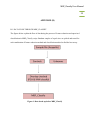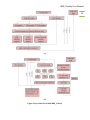
1
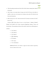
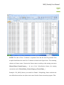
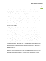
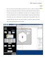
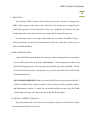
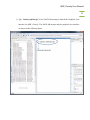
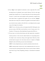
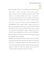
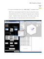
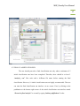
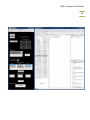
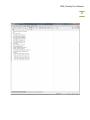
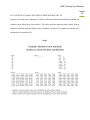
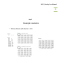
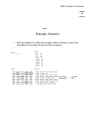
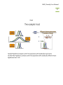
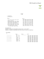
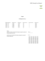
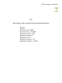
MBF_CLASSIFY USER MANUAL Mac Biophotonics Facility MBF_Classify User Manual 2 CONTENTS 1. Introduction 3 2. What will the software do? 3 2.1 Initial Classification runs 3 2.2 Final Classification run 5 3. What it will not do. 5 4. Protocol 10 4.1 Pre classification 10 4.2 Initial Classification run 10 4.3 Final Classification run 17 5. Classification Interface for Different Controls and Test Sets 21 6. Interpretation of Results 21 7. Appendix (A) 28 8. Appendix (B) 32 MBF_Classify User Manual 3 1. INTRODUCTION Machine learning is a technique that can provide good classification results for objects seen in microscopic images. There exist many methods by which machine learning can be accomplished and every method makes use of a supervised classifier. A supervised classifier takes a training set consisting of examples of each class and assigns a particular class to an unknown input. MBF_Classify is based on the same approach and uses three supervised clustering methods namely KNN (K Nearest Neighbors), SVM (Support Vector Machines) and Neural Network to generate classes for every unknown object in the data set. However, MBF_Classify can also be used to collate a training set from a mixed population of images without the user having to manually assign a class to the images. 2. WHAT WILL THE SOFTWARE DO? 2.1 INITIAL CLASSIFICATION RUNS MBF_Classify allows the user to run a series of classifications over the same data set and save the results for later use. It systematically cycles through different samples of control objects, feature reduction algorithms, number of features kept from the feature reduction, and classifiers. The best performing classification scenario for the given control data set is identified and applied to cluster the unknown data. The underlying algorithm of MBF_classify is based on the idea of systematically testing all the possible classification scenarios applied to the control data and then picking the optimal scenario. Although the MBF_Classify User Manual 4 optimal scenario is selected each initial classification run uses only a selection of the control data. Therefore, when the data set is large enough several different initial classifications should be used to identify the most robust feature set. There are 4 variables in each classification scenario: 1) The size of the control set (values from 25 to a user defined number in steps of 25), 2) Feature reduction method (PCA, KS, SDA), 3) Number of features to keep after feature reduction, and 4) The classification method (KNN, SVM, Neural Network). The algorithm selects one process from each step (e.g. for the feature reduction step it will choose one of PCA, KS or SDA as a process) to train and test a classifier. The accuracy of the classifier is calculated from the test results and is stored for later use. This process is repeated for the same scenario for a user defined number of replicates. Thus, a series of accuracy values for each possible scenario is recorded. From these accuracy values, an optimal scenario is chosen and then this optimal scenario is used to create a classifier in a final classification stage (see below) and classify the unknown data. NOTE: KS and SDA are the most frequently used feature reduction methods by MBF_Classify. It has also been observed that supervised clustering is usually performed by using KNN and SVM and very rarely Neural Networks. However, when using 3 controls, KNN is the most preferred method followed by Neural Networks. SVM is rarely used for 3 controls. MBF_Classify User Manual 5 2.2 FINAL CLASSIFICATION RUN Following the analysis of the dataset for a number of times, the user can move ahead to final classification run. During the final run, the software picks only those features that have been used at least 60 % of the times during the initial classification runs of the same dataset and performs a final classification of the dataset. It goes through the same protocol of feature reduction and classification as described for the initial classification result. The results are also saved in the same manner for later use. 3. WHAT IT WILL NOT DO. The software will not substitute for inaccurate input data. MBF_Classify works only if the data is generated in a certain format from Acapella. The figure below shows the snapshot of a typical data file as per the Acapella script used. The rows in the data file correspond to the objects to be classified. First 15 columns in the data file represent the experimental information and the remaining columns correspond to the features extracted through image analysis. NOTE: If the software shows an error saying “File not in standard format”, the user can take the following actions: Check the first 15 columns of the file generated from Acapella. These columns should correspond to the experimental information in the same order as shown in the figure, the eighth column being the treatment sum information. MBF_Classify User Manual 6 Check the naming convention used in the file for all the features starting from column 16 and onwards. Check if there are too many clusters of empty rows in the file. However, the software is capable to remove one or two empty rows occurring at some points. This feature has not been tested exhaustively. Make sure there are no “Inf” values in the data file. The software can deal with “NaN’s” but not “Inf’s”. Currently, MBF_Classify allows the user to select between 3 channels (Channel1, Channel2, and Channel3) and 4 feature categories (Morphology, Intensity, Texture, and Colocalization). The nomenclature followed in the data file shown in the following figure is as follows: Ch1: Channel 1 Ch2: Channel 2 Ch3: Channel 3 MOR: Morphology INT: Intensity TXT: Texture CLC: Colocalization NOTE: MATLAB is case sensitive so upper case letters cannot be replaced by lower case letters and vice versa. MBF_Classify User Manual 7 NOTE: The order of first 15 columns is important. Note that the data file generated from Acapella should have the same first 15 columns as shown in the figure above. The remaining columns are feature names. Generate the feature names according to the naming convention ChannelName_FeatureCategory_.... In case of the Colocalization feature, the naming convention used is ChannelName_FeatureCategory_ChannelName_.... Examples: Ch1_MOR_Nucleus_area stand for Channel 1 Morphology feature and then the user defined term nucleus area (these terms come from the feature extraction program). That MBF_Classify User Manual 8 the last part of the name is not fixed permits features to be added or deleted as desired. Ch1_CLC_Ch2_ICQ stands for Channel 1 Colocalization with Channel 2 and in this case indicates that the colocalization feature was an ICQ calculation. While selecting the channels, the user should take care which channel number corresponds to which color and include only the channels that are required for classification. The user has the option of selecting all three channels or just the two channels required for classification as per the requirements of the experiment. The software also allows the user to select only a single channel. MBF_Classify has been designed to perform classification using either 2 or 3 controls for training the classifiers. The user must take care that anything other than 2 or 3 controls is not allowed and would generate an error. Also, the software cannot proceed to classification if the controls provided for training have a very high degree of overlap. MBF_Classify provides an approximate demonstration of the amount of overlap in the controls by plotting them in Principle Component Space as shown in the following figure. The approximate percentage of the overlap is also displayed at the top of the PCA plot for the user. A pop up error message also shown, indicates the user to check the controls if it finds them with high amount of overlap. The amount of overlap that is allowed to proceed for classification is anything less than 50%. NOTE: The software has been designed to take care of high overlaps by stopping them from entering the classification process However, in some cases the data might have an overlap MBF_Classify User Manual 9 that is just below 50% but the controls are positioned in such a way that a fair amount of demarcation is not possible. In such a case the software might enter the classification process but report later at the time of classification in the form of an error dialogue box that no feature was found by any of the feature reduction methods to separate the controls. In cases where there is too much overlap because the treated control is heterogeneous (some cells responded and others did not) it may still be possible to classify the images but a KNN single control (described below) may be required. MBF_Classify User Manual 10 4. PROTOCOL The working of MBF_Classify can be divided into two parts. The first is setting up the MBF_Classify inputs in the correct order followed by the second part of employing the classification process. For the convenience of the user, a graphical user interface has been designed that allows the selection of the correct inputs for the classification process. As mentioned earlier, a two stage classification run is possible with MBF_Classify – Initial classification run and Final classification run. Both the stages have similar steps to follow as mentioned below. 4.1 PRE CLASSIFICATION Open MATLAB and set the path of the directory where the program files (.m extension) are saved. The path can be set by using “File\set path…” and navigating to the folder with the MATLAB program files. This step needs to be followed only when using MBF_Classify on MATLAB for the first time. The path once set is saved in the pathdef.m file of MATLAB for all subsequent runs. MATLAB REQUIREMENTS: Make sure that the MATLAB version being used has the 3 toolboxes installed before using the software: Neural Network toolbox, Statistics toolbox, and Bioinformatics toolbox. To check the version and toolboxes present in the MATLAB version being used, type “ver” and press enter on the MATLAB prompt. 4.2 INITIAL CLASSIFICATION RUN Once the path has been set, the user can start using the software for classification. Follow the steps mentioned below to proceed: MBF_Classify User Manual 11 1) Type “initiate_mbfclassify” at the MATLAB prompt to launch the Graphical User interface for MBF_Classify. The MATLAB prompt and the graphical user interface are shown in the following figure. MBF_Classify User Manual 12 2) Press “Single” on the Graphical User Interface to select a single data file on which the analysis has to be performed, from its specific directory. This file is the output generated from Acapella with “.txt” extension and needs to be in the format specified in section 3. At times, there can be multiple text files generated by Acapella for the same dataset. Hence, to append the files together, the user can hit the “Multiple” button and select as many files as needed to be appended. Once the data file (files) is (are) selected, the name (number) of the file (files) is (are) displayed on the top right corner of the Graphical User Interface. NOTE: The size of the data set that can be imported into MATLAB depends on the processor memory. MATLAB can crash and show an error if memory space is low. Generally, a 32 bit processor will not handle data files greater than 2GB in size. 3) The next step is to select the desired features and what channels they correspond to. General procedure is to first select the channel and then its corresponding features. The channel can be selected by clicking on the toggle button followed by feature selection from the respective list. Once feature selection is complete, hit “Features Selected” to allow MATLAB to process the selected information. NOTE: To select multiple features press control key and make selection from list. NOTE: Advanced feature selection tool is also included that allows the user to be even more specific in selecting features. Hence, the user can select features within the major classes of type Texture, Morphology, Intensity or Colocalization as mentioned earlier. MBF_Classify User Manual 13 4) Once the processing is complete a list of treatments used in the experiment appears under “Control 1”, “Control 2” and “Control 3”. The user can now specify the number of controls to be used for classification and select the respective controls from the list. Two different treatments under “Control 1” and “Control 2” respectively, should be selected if the user wants to proceed into classification using only 2 controls while for classification with 3 controls, three different treatments under “Control 1”, “Control 2” and “Control 3” respectively, should be selected. Hit “Controls selected” once the selection of controls is complete. The software also allows the user to upload the specific objects as the controls and proceed towards classification. The control objects to be uploaded should be mat files (extension: .mat). 2 mat files need to be uploaded for running a classification with 2 controls while 3 files need to be uploaded if the user wants to run a three way classification. The specific objects can be selected and saved into mat files using the knn single control algorithm as discussed in Appendix. NOTE: Before proceeding towards the selection of controls, make sure the “number of controls” box has been set to the correct number. For example: 2 for selecting two controls and 3 for selecting three controls. For a three control classification, if the user does not change the number of controls to 3 and proceeds towards selecting three treatments per control, the software would completely ignore the third control selected and perform classification using only the first two controls. MBF_Classify User Manual 14 5) To start the classification process, hit “MBF_Classify”. As mentioned earlier, MBF_Classify starts checking the controls for the degree of overlap. If the overlap is in permissible limits (below 20 %), it asks the user to input the values for “Maximum Controls”, “Maximum Features” and “Repetitions”. The window to input values along with the figure for overlap in the controls is shown in the figure below. MBF_Classify User Manual 15 NOTE: Controls are selected starting with 25 and stepping up by 25. Default value is set to 100 and generally is a good number for training the classifier. The maximum features to be used must be less than the total features, but in practice, typical values are 15 or less- this allows the computations to be completed in a reasonable length of time. However, the default value has been set to 15. The number of repetitions is exactly the number of times MBF_Classify will cycle through the training and classification process for a given number of controls, feature reduction, number of features and classifier scenario. In practice, 10 repetitions which is the default value, work well without causing the program to require great length of time. NOTE: The processing times for classification can range from 30 minutes to 6 hours depending on the size of the data set, the total number of features in the set, and the number of repetitions chosen by the user. The processing time can also increase marginally in case of a very high overlap between the controls (approximately between 40 to 50 %) 6) Once the classification is complete, MBF_Classify prompts the user to save the results. The users are encouraged to save the names with experiment number after the underscore to keep track for later use, especially when doing the optional final classification run. The data from these initial classifications can be viewed and used as is. The output is in the same format as the output for the final classification run (see below for how to view and interpret this data). In the initial classification runs PCA can be used as the feature reduction method and to view the data. However, the MBF_Classify User Manual 16 output will not include a list of the specific features used as the PCA process combines them linearly. The program permits PCA classification for those users that wish to stop at this stage and not perform a final classification run. Data generated using PCA cannot be used in the final classification because the features are not specified explicitly. However, if MBF_Classify picks up PCA as the best feature reduction method, it would immediately prompt the user as shown in the figure below to chose between carrying on with PCA in which case no feature list would be available or switch to the next best feature reduction method but PCA that was picked after statistical analysis and get the feature list. NOTE: The instructions to use the Graphical User Interface mentioned above also appear at the bottom of the interface as the user proceeds. 7) To run another initial classification, close the interface and repeat steps 1 to 5. MBF_Classify User Manual 17 4.3 FINAL CLASSIFICATION RUN The user should proceed to final classification run only when a minimum of 5 initial classification runs have been completed. Therefore, there should be at least 5 “analysis_....txt” files each with a different file name before running the final classification. However, 10 initial classification runs are highly recommended. The user can enter the final classification run interface via two routes. First, by clicking on the pushbutton at the bottom right corner of the initial classification run interface named “Proceed to final analysis” or second, by typing “initiate_mbffinalrun” on the MBF_Classify User Manual 18 MATLAB prompt. Both these steps would open the final classification run interface as shown in the following figure. The steps needed to be followed are as follows: 1) Press “Single” or “Multiple” on the Graphical User Interface to select a single data file or multiple data files, respectively on which the analysis has to be performed, from its specific directory in the manner similar to the one used for the initial classification run. This file is the output generated from Acapella with “.txt” extension and needs to be in the format specified in section 3. Once the data file is selected, the name of the file is displayed on the top right corner of the Graphical User Interface. 2) Press “Select analysis files” to select the analysis files generated from initial classification run. This button allows the user to select multiple files at the same time by using ctrl or shift keys. Once the set of analysis files have been selected, the corresponding names appear under “Analysis file names”. The interface would automatically update the list of top features that repeated at least 60 % of the times under the title “Feature names”. The user can then select all features in the list or only the top few features to conduct the classification on. Once the feature selection has been made, hit “Selected”. NOTE: If no feature names appear, please re check the files used for analysis. The possible reasons are that there are no features in common or the initial analysis runs MBF_Classify User Manual 19 used PCA as feature reduction method. In either case, try running a few more classification runs to see if any features appear to be commonly used. NOTE: Multiple feature selection can be done using the ctrl or shift keys. NOTE: The feature names are arranged in descending order and appear with their respective hit rate as a percentage. A hit rate of 100% means that the particular feature was repeated in all the initial runs and should certainly be used for the final classification run. 3) Once the feature selection is complete, the steps are the same as steps 4 to 6 for the initial classification run explained in Section 4.2. NOTE: While setting the parameters for final classification run, the user must make sure that the “Maximum Features” input should not exceed the number of features selected under the title “Feature names”. The default value for “Maximum Features” is automatically updated to the number of features selected by the user under the title “Feature names”. It is recommended to perform the classification run using the default values. NOTE: The software does not allow the user to select three or less than three features for the final classification run. MBF_Classify User Manual 20 MBF_Classify User Manual 21 5. CLASSIFICATION INTERFACE FOR DIFFERENT CONTROLS AND TEST SETS There can be cases when the user wants to try a particular set of controls from one data set to classify another set of objects coming from a different data set. Hence, another interface has been designed that allows the user to upload two different text files as the files from where the control set and the test set would be selected, respectively. The protocol to use this interface is similar to the protocol used to run MBF_Classify except for a few changes. 1) Type “initiate_mbfclassify_diff” at the MATLAB prompt to launch the Graphical User Interface. The MATLAB prompt and the graphical user interface are shown in the following figure. 2) As mentioned for MBF_Classify, the user can upload a single data file or multiple data files by clicking on the “single” or “multiple” buttons. However, in this case, the user has to upload two different files or two different sets of files as control and test, separately. 3) The steps ahead of this that is the selction of features and channels, followed by the selection of controls are the same as described for MBF_Classify earlier. 6. INTERPRETATION OF RESULTS The results of both initial classification run and final classification run consist of two types of files that appear in the “current folder” panel of MATLAB. First is a “.fig” file that contains the PCA plot of the controls used for classification of the data. Second is another “.fig” file that contains the controls and unknowns classified plotted together in the PCA plot. The third file is a “.dat” file that contains the classification results for the test data. The results are saved in two parts (described below). Apart from saving the MBF_Classify User Manual 22 results, another “.dat” file is created that saves the information corresponding to the “controls” used for classification. All these “.dat” files can be opened in MATLAB by right clicking on them and selecting the option of “open as text” or as excel file, word file or using WordPad. The first “.dat” file is labeled as “results_” and includes the following information: 1) FEATURE REDUCTION METHOD: This specifies which method was used for feature reduction before proceeding into classification by MBF_Classify. It can show KS, SDA or PCA as the feature reduction method used. 2) FEATURES USED: The names of the features that were used for classification are specified under this heading. NOTE: The feature names are displayed only in the case when KS or SDA have been used as feature reduction methods. However, in case of PCA, no feature names are displayed. This is because PCA uses a combination of various features for classification and not singular discrete features as in the case of SDA and KS feature reduction methods. 3) TREATMENTS: This lists the set of all the treatments used in the data set being analyzed. The controls used for the analysis had been selected from the same list of treatments. 4) SCORES: This gives the scores of the number of objects classified as either of the controls selected earlier. The scores is a matrix with either three or four columns depending on the number of controls used for classification and rows corresponding MBF_Classify User Manual 23 to the number of treatments present. In case of two controls, the matrix consists of three columns where the first column gives the total number of objects per treatment, the second column represents the number of objects classified as control 1 per treatment and the third column gives the number of objects classified as control 2 for each treatment. However, in case of three controls, there are four columns in the matrix. The first column being the total number of objects per treatment, second being the number of objects classified as control 1, third being the number of objects classified as control 2 while the last column gives the number of objects classified as control 3 per treatment. Each treatment is presented on a separate row. However, the second “.dat” file is labeled as “coordinates_” and includes the information for each cell that was classified as either of the controls selected”: 5) The above mentioned variables are followed by a set of variables arranged in a matrix form. The first column in the matrix corresponds to the WELL NUMBER, second column specifies the PLATE ID, third column represents the IMAGE NUMBER, fourth column corresponds to the CONTROL, fifth column representing the FIELD OF VIEW, sixth and seventh columns are for X- COORDINATES and YCOORDINATES of the object being classified and the last or eighth row specifies the classification result of the cell. MBF_Classify User Manual 24 The third “.dat” file consists of the same information as stored in “coordinates_” except that the file is named “controls_” and shows the information corresponding to the controls used for classification. The following figure shows the three “.dat” files created after the initial classification run. Similar files are created after the final classification run. NOTE: For files named “coordinates_” and “controls_” the last column that is the class category, 1 represents the type of object selected as control 1, 2 represents the type of object selected as control 2 and 3 if present, represents the type of object selected as control 3. MBF_Classify User Manual 25 MBF_Classify User Manual 26 MBF_Classify User Manual 27 NOTE: This file can be used by Acapella directly to look at the images of the classified cells. MBF_Classify User Manual 28 APPENDIX (A) A.1 KNN SINGLE CONTROL ALGORITHM While working with high content screening data, there can be situations when only a single control is present to create a classifier. For example, the single control can be the set of objects that were not affected by a particular treatment and hence, can be called a negative control. In order to proceed towards classification using MBF_Classify, there is a requirement of at least 2 controls. Hence, software called KNN single control was designed that performs a comparison between the single control, usually the unaffected objects and all the other objects in the population to pick those objects as the second control that are most distinct from the unaffected population. This is done by comparing the distances from the unaffected population to a benchmark to the distances of a given query to the benchmark using the KS test. The classification procedure described above often fails if more than 50% of the „treated control‟ cells were unaffected. In this situation the „treated control‟ is not really an appropriate control. To create a more useful control set we created the KNN single control algorithm. Using this algorithm the user selects from the treated cells those that are significantly (we usually use p = 0.1) different than the normal cells. This group of cells is then used as the positive control in the classifier. The alternative, and what other software programs do, is to let the user manually select positives based on visual inspection. At the moment we do not favor this approach but if you want to use it there is a way to do it. To manually select positive controls one selects them using Acapella and then uses the feature extraction script to extract the features from the selected cells. These are then provided to MBF_classify as a positive control set. MBF_Classify User Manual 29 A.2 PROTOCOL The KNN one control algorithm can be launched through MATLAB in a similar way as described for the other user interfaces above. 1) Type “initiate_knnonecontrol” on the command prompt to launch the interface. The figure below shows the command to launch the interface along with the interface. MBF_Classify User Manual 30 2) Once the interface opens, the user can select a single file to upload by clicking in the “single” button or upload multiple files that would be appended together by hitting the “multiple” button. The name of the file appears on the interface once it is done uploading it. 3) The next step is to select the single control from the list that appears in the select control column. The list appears automatically once the upload of the file is complete. NOTE: That while multiple sets of data can be analyzed to generate a control set only a single control can be selected from the list for each analysis. 4) The user then has the option of either plotting the distributions of the distances of the control and the samples from the benchmarks (if you want to visually determine how overlapping the distributions are) or directly starting the analysis by clicking on the “KNN one control” button. NOTE: Since KNN computes an average distance of K number of nearest neighbors to the benchmark object, there has been included an option to specify the number of nearest neighbors that should be used for the analysis by the user. 5) A new pop-up box appears in which the user enters the p value for the analysis (the default is 0.1). In practice we have found 0.1 the best but values between 0.05 and 0.5 all work to varying degrees. 6) In performing the analysis the program analyzes the untreated cells and determines the distribution for all of the cells based on all of the features (it uses all the features in the data files). It then uses a random set of cells from the untreated control as a benchmark. MBF_Classify User Manual 31 In the next step the program measures the distance of all of the objects (cells) in the treated samples from the benchmark. Once the analysis is complete, the KNN one control algorithm creates as many “control/sample… .mat” files as there are treatments present in the “Select Control” column on the interface. The “control/sample… .mat” files contain the information of the objects picked as control as specified by the user and the objects (cells) in the treatments that are scored as affected by comparing to the p value selected above (usually 0.1). These objects can therefore be used as the second control to perform analysis in MBF_Classify by simply uploading the “control/sample_… .mat” files on the interface. If there are multiple .mat files they can be appended to each other in the main part of MBF_classify. MBF_Classify User Manual 32 APPENDIX (B) B.1. DATA FLOW THROUGH MBF_CLASSIFY The figures below explain the flow of data during the process of feature reduction and supervised classification in MBF_Classify script. Random samples of equal sizes are picked and tested for each combination of feature reduction method and classification method to find the best set up. Figure 1: Data break up before MBF_Classify MBF_Classify User Manual 33 (a) (b) Figure 2(a,b): Data flow within MBF_Classify MBF_Classify User Manual 34 B.2. STATISTICAL ANALYSIS STEPS TO FIND THE BEST SET UP In order to select the best combination of feature reduction method and classification method, the statistical steps followed are shown below. The values used here represent actual values from an analysis performed using the default values of number of features (15), number of controls (100) and number of repititions (10). Step 1 MBF_Classify User Manual 35 Step 2 MBF_Classify User Manual 36 Step 3 MBF_Classify User Manual 37 Step 4 MBF_Classify User Manual 38 Step 5 MBF_Classify User Manual 39 Step 6 MBF_Classify User Manual 40 Step 7