1
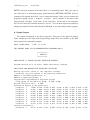
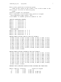
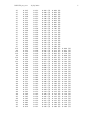
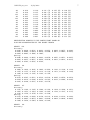
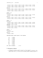
COPOPS program
27/08/2010
1
COPOPS User’s Guide
1. Description
COPOPS is a FORTRAN77 program that implements a decision aid for obtaining
Pareto-optimal predictor subsets as described in De Corte, Sackett and Lievens (2010).
The executable code is offered as is, without any guarantee whatsoever.
Executing the code requires a key that can be obtained by mailing to the first
author.
The present program is limited to the followed conditions: (a) two selection goals,
(b) the total number of feasible predictor subsets may not exceed 500, (c) only one
minority group and only one job performance criterion, and (d) the maximum number
of computed trade-offs per subset is 50.
Observe that the program is computationaly very complex. Even with the
above limitations, the execution time may take several minutes of CPU time, depending
on the floating point performance of the computer.
2. Input
Note that all input is in free format: Variables or vectores that have a name
commencing with the letters I, J, K, L, M, N get INTEGER values. All other
variables, vectors and matrices get FLOATING POINT values. See the example
input file.
• # 0: KEY
• # 1: ITY, NP, IFWE, IBN
– ITY: Controls the metric used to translate the selection quality and the selection diversity goal.
ITY = 0: quality corresponds to expected job performance and diversity
refers to the adverse impact ratio.
ITY = -1: quality corresponds to the composite validity and diversity refers
to the minority selection rate.
– NP: total number of predictors (NP ≤ 10)
– IFWE: IFWE controls the weighting of the predictors when forming composites. If IFWE = 0 then optimal weighting; if IFIWE = 1 then regression
weighting; if IFIWE = 2 then unit weighting
– IBN: IBN controls the number of Pareto-optimal solutions computed for each
feasible predictor subset. The value of IBN must be between 10 and 50.
Recommended value is 20.
COPOPS program
27/08/2010
2
• # 2: NRWE, WMA. Only required if IFIXWE = 0!!
– NRWE: If NRWE = 0, then the predictor weighting when forming predictor
composites must obey a ratio constraint. No such ratio constraint if NRWE
= 1.
– WMA: The ratio between the largest and the smallest predictor weight when
forming composites must be between 1/WMA and WMA. If NRWE = 1, a
value for WMA must be specified, but the value is ignored.
• # 3: SELR, COLIM, PMIN, CESMIN
– SELR: Selection ratio of the selection
– COLIM: Maximum total predictor costs
– PMIN: proportion of minority applicants in the total applicant group
– CESMIN: Criterion effect size (i.e., mean difference on the performance criterion between the minority and the majority applicant populations. If the
mean criterion performance in the minority population is less than the mean
performance in the majority population then CESMIN should have a NEGATIVE value; positive otherwise.
• #4: PESMIN(I), I = 1, NP
Vector of length NP with the effect sizes of the available predictors (all effect sizes
are for the minority population relative to the majority population).
• #5 and following NP-2 lines: Set of NP-1 lines specifying CP(I,J) (with I =
1, NP-1 and J = I+1, NP) the correlation matrix of the NP predictors.
Note that the strict upper diagonal part of the correlation matrix must be specified!
(see example)
• #6: PVAL(I), I = 1, NP
Vector of length NP with the validities of the available predictors
• #7: PCOST(I), I = 1, NP
Vector of length NP with the predictor cost PER APPLICANT of the available
predictors
• #8 MIP, MAP
MIP: the minimum number of predictors that must be used in the composite; and
MAP: the maximum number of predictors that can be used in the composite.
COPOPS program
27/08/2010
3
• #9: ISP(I), I = 1, NP
Vector of length NP with values of 0, 1, or 2. ISP(I) = 0 indicates that predictor
I can not be used; a value equal to 2 indicates that the predictor must be used; a
code equal to 1 indicates that the predictor can be used.
4. Sample Input File
Important: in preparing the input file, use a simple text editor such as Notepad,
Wordpad or any other standard ASCII producing editor. DO NOT USE TEXT PROCESSING PROGRAMS SUCH AS MS-WORD or WORDPERFECT. Also, when saving
the input file in Notepad, use the option “All Files” in the “Save as type” box. When
saving in Wordpad, use the “Text Document-MS-DOS Format” option in the “Save as
type” box, and be aware that Wordpad has the nasty habit of adding the extension .txt to the file name that you specify. Thus, with Wordpad, if you specify the
name of the input file as “MINPUT”, the file will in fact be saved as “MINPUT.TXT”;
and this is the name that you have to use in the command to run the present programs.
Here is a sample input file, for the copops program.
KEY
-1 9 0 20
0 10.
0.30 100. 0.20 -0.0
-1.008 -0.725 -0.684 -0.162 -0.992 -1.213 -0.797 -0.602
0.598 0.780 0.467 0.596 0.593 0.649 0.430 0.272
0.629 0.694 0.620 0.432 0.516 0.532 0.373
0.475 0.561 0.506 0.622 0.426 0.337
0.413 0.090 0.335 0.456 0.415
0.725 0.642 0.574 0.192
0.757 0.348 0.029
0.398 0.169
0.294
0.522 0.545 0.561 0.407 0.545 0.529 0.525 0.442
0.341
20. 10. 20. 10. 10. 15. 15. 20. 25.
1 3
1 1 1 1 1 1 1 1 1
-0.178
5. Running the Program
Suppose you copied the executable code of the program to the C:ssel directory on
your machine. In that case, the input file must also be saved in the C:ssel directory.
Next, to run the program, you have to open an MS-DOS Command window. The way
to do this varies from one operating system (i.e., XP, Vista, Windows 7 a.s.o.) to the
other, and you should use your local “HELP” button when in doubt about this feature.
If the MS-DOS Command window does not automatically open with the prompt
C:\>, then you type in the MS-DOS Command window C:, followed by RETURN or
COPOPS program
4
27/08/2010
ENTER, and your computer will return the C:\> command prompt. Next, you type cd
ssel after the C:\> command prompt, again followed by RETURN or ENTER, and your
computer will respond with the C:\ssel> command prompt. Now, you can execute the
program by typing copops < minput > moutput
where “minput” is the name of the
input file and “moutput” is the name of the output file. At the end of the execution,
the PC will return the command prompt C:\ssel>. You can then inspect the output by
editing the output file with either Notepad, Wordpad or any other simple editor program.
6. Sample Output
The output corresponds to the above input file. Only part of the output is printed.
Other examples of the input and corresponding output files are available at the URL
that contains the executable program.
DATE: 26/08/2010;
TIME: 11:11:46
THE PRESENT CODE IS FOR DEMONSTRATION PURPOSES ONLY!!
+++++++++++
+ COPOPS +
+++++++++++
COMPUTATION of PARETO-OPTIMAL PREDICTOR SUBSETS
Program written by W. De Corte, Ghent University, Belgium
INPUT DATA AND DESCRIPTION SELECTION SITUATION
Quality objective refers to the composite validity
Diversity objective refers to the minority hiring rate
Number of available predictors: 9
Number of applicant groups: 2
Proportional representation applicant groups
First group is the Minority group: 0.200 0.800
Overall selection ratio: 0.300
Correlation matrix of the predictors:
Predictor 1
1.000 0.598 0.780 0.467 0.596 0.593
Predictor 2
0.598 1.000 0.629 0.694 0.620 0.432
Predictor 3
0.780 0.629 1.000 0.475 0.561 0.506
Predictor 4
0.467 0.694 0.475 1.000 0.413 0.090
Predictor 5
0.596 0.620 0.561 0.413 1.000 0.725
Predictor 6
0.593 0.432 0.506 0.090 0.725 1.000
Predictor 7
0.649 0.516 0.622 0.335 0.642 0.757
Predictor 8
0.430 0.532 0.426 0.456 0.574 0.348
Predictor 9
0.272 0.373 0.337 0.415 0.192 0.029
Predictor Validities:
Criterion 1
0.522 0.545 0.561 0.407 0.545 0.529
0.649
0.516
0.622
0.335
0.642
0.757
1.000
0.398
0.169
0.430
0.532
0.426
0.456
0.574
0.348
0.398
1.000
0.294
0.272
0.373
0.337
0.415
0.192
0.029
0.169
0.294
1.000
0.525
0.442
0.341
COPOPS program
5
27/08/2010
Effect sizes predictors in Minority group:
-1.008 -0.725 -0.684 -0.162 -0.992 -1.213 -0.797 -0.602 -0.178
Effect sizes criterion in Minority group:
0.000
Predictor weights are optimized
Ratio constraint on the within stage predictor weights:
Max weight/Min weight equals 10.0
Total number of feasible predictor subsets is: 129
IDENTITY PREDICTOR SUBSETS
Subset
1: Predictors 1
Subset
2: Predictors 2
Subset
3: Predictors 3
Subset
4: Predictors 4
Subset
5: Predictors 5
Subset
6: Predictors 6
LINES DELETED
Subset 126: Predictors 6
Subset 127: Predictors 6
Subset 128: Predictors 6
Subset 129: Predictors 7
7
7
8
8
8
9
9
9
SORTED PARETO OPTIMAL QUALITY FOR PLOT USING R
0.4070, 0.4219, 0.4235, 0.4250, 0.4266, 0.4281,
0.4326, 0.4341, 0.4356, 0.4370, 0.4385, 0.4399,
0.4439, 0.4452, 0.4463, 0.4474, 0.4483, 0.4488,
0.4561, 0.4626, 0.4644, 0.4674, 0.4744, 0.4788,
0.4981, 0.5059, 0.5136, 0.5212, 0.5287, 0.5362,
0.5577, 0.5646, 0.5712, 0.5775, 0.5833, 0.5886,
0.5951, 0.5984, 0.6018, 0.6084, 0.6144, 0.6158,
0.6246, 0.6305, 0.6332, 0.6415, 0.6494, 0.6567,
0.6648, 0.6664, 0.6690,
0.4296,
0.4413,
0.4496,
0.4824,
0.5435,
0.5929,
0.6194,
0.6574,
0.4311,
0.4426,
0.4530,
0.4903,
0.5507,
0.5948,
0.6208,
0.6630,
SORTED PARETO OPTIMAL DIVERSITY FOR PLOT
0.2562, 0.2536, 0.2533, 0.2530, 0.2527,
0.2515, 0.2512, 0.2509, 0.2506, 0.2503,
0.2489, 0.2486, 0.2482, 0.2478, 0.2473,
0.2394, 0.2383, 0.2379, 0.2360, 0.2354,
0.2240, 0.2202, 0.2163, 0.2123, 0.2083,
0.1916, 0.1872, 0.1827, 0.1779, 0.1729,
0.1544, 0.1539, 0.1529, 0.1474, 0.1415,
0.1320, 0.1255, 0.1251, 0.1179, 0.1105,
0.0925, 0.0833, 0.0810,
0.2521,
0.2496,
0.2404,
0.2317,
0.2001,
0.1616,
0.1349,
0.1016,
0.2518,
0.2493,
0.2396,
0.2279,
0.1959,
0.1582,
0.1329,
0.0939,
USING R
0.2524,
0.2499,
0.2468,
0.2318,
0.2043,
0.1676,
0.1389,
0.1026,
SUMMARY TABLE SELECTED PARETO-OPTIMAL SYSTEMS AND TRADE-OFFS
Subset
4
35
35
Quality
0.407
0.422
0.423
Diversity
0.256
0.254
0.253
Predictor weights
0.407 (4)
0.404 (4) 0.040 (9)
0.403 (4) 0.045 (9)
COPOPS program
35
35
35
35
35
35
35
35
35
35
35
35
35
35
35
35
35
35
35
119
99
119
119
99
119
99
118
99
99
99
99
99
99
99
99
99
99
99
99
99
99
99
99
99
97
99
118
97
97
97
0.425
0.427
0.428
0.430
0.431
0.433
0.434
0.436
0.437
0.438
0.440
0.441
0.443
0.444
0.445
0.446
0.447
0.448
0.449
0.450
0.453
0.456
0.463
0.464
0.467
0.474
0.479
0.482
0.490
0.498
0.506
0.514
0.521
0.529
0.536
0.543
0.551
0.558
0.565
0.571
0.577
0.583
0.589
0.593
0.595
0.595
0.598
0.602
0.608
0.614
6
27/08/2010
0.253
0.253
0.252
0.252
0.252
0.252
0.251
0.251
0.251
0.250
0.250
0.250
0.249
0.249
0.249
0.248
0.248
0.247
0.247
0.240
0.240
0.239
0.238
0.238
0.236
0.235
0.232
0.232
0.228
0.224
0.220
0.216
0.212
0.208
0.204
0.200
0.196
0.192
0.187
0.183
0.178
0.173
0.168
0.162
0.158
0.154
0.154
0.153
0.147
0.141
0.402
0.400
0.399
0.398
0.396
0.394
0.392
0.390
0.387
0.384
0.381
0.377
0.373
0.368
0.363
0.356
0.348
0.337
0.321
0.398
0.041
0.386
0.361
0.040
0.334
0.039
0.351
0.052
0.066
0.080
0.095
0.111
0.128
0.146
0.165
0.185
0.206
0.228
0.251
0.277
0.304
0.334
0.366
0.404
0.265
0.451
0.251
0.274
0.283
0.292
(4)
(4)
(4)
(4)
(4)
(4)
(4)
(4)
(4)
(4)
(4)
(4)
(4)
(4)
(4)
(4)
(4)
(4)
(4)
(4)
(3)
(4)
(4)
(3)
(4)
(3)
(4)
(3)
(3)
(3)
(3)
(3)
(3)
(3)
(3)
(3)
(3)
(3)
(3)
(3)
(3)
(3)
(3)
(3)
(3)
(3)
(4)
(3)
(3)
(3)
0.050
0.056
0.061
0.067
0.072
0.078
0.085
0.091
0.098
0.105
0.113
0.121
0.129
0.138
0.148
0.159
0.172
0.187
0.208
0.040
0.413
0.039
0.036
0.395
0.041
0.348
0.040
0.347
0.346
0.344
0.342
0.339
0.334
0.329
0.323
0.316
0.308
0.298
0.286
0.273
0.257
0.237
0.214
0.183
0.327
0.138
0.351
0.309
0.287
0.260
(9)
(9)
(9)
(9)
(9)
(9)
(9)
(9)
(9)
(9)
(9)
(9)
(9)
(9)
(9)
(9)
(9)
(9)
(9)
(8)
(4)
(8)
(8)
(4)
(8)
(4)
(7)
(4)
(4)
(4)
(4)
(4)
(4)
(4)
(4)
(4)
(4)
(4)
(4)
(4)
(4)
(4)
(4)
(4)
(4)
(4)
(7)
(4)
(4)
(4)
0.066
0.041
0.099
0.150
0.096
0.189
0.181
0.192
0.182
0.184
0.185
0.186
0.186
0.186
0.186
0.186
0.185
0.184
0.182
0.179
0.176
0.171
0.166
0.158
0.148
0.136
0.132
0.210
0.157
0.180
0.205
(9)
(9)
(9)
(9)
(9)
(9)
(9)
(9)
(9)
(9)
(9)
(9)
(9)
(9)
(9)
(9)
(9)
(9)
(9)
(9)
(9)
(9)
(9)
(9)
(9)
(7)
(9)
(9)
(7)
(7)
(7)
COPOPS program
96
97
116
96
116
96
96
96
96
116
96
116
96
116
0.616
0.619
0.621
0.625
0.630
0.633
0.642
0.649
0.657
0.657
0.663
0.665
0.666
0.669
7
27/08/2010
0.139
0.135
0.133
0.132
0.125
0.125
0.118
0.110
0.103
0.102
0.094
0.092
0.083
0.081
0.311
0.301
0.385
0.310
0.379
0.307
0.303
0.296
0.287
0.343
0.273
0.318
0.247
0.274
(3)
(3)
(4)
(3)
(4)
(3)
(3)
(3)
(3)
(4)
(3)
(4)
(3)
(4)
0.347
0.223
0.273
0.343
0.301
0.338
0.332
0.322
0.309
0.399
0.289
0.442
0.255
0.498
(4)
(4)
(6)
(4)
(6)
(4)
(4)
(4)
(4)
(6)
(4)
(6)
(4)
(6)
0.120
0.236
0.246
0.145
0.247
0.172
0.202
0.235
0.273
0.239
0.319
0.231
0.381
0.213
(6)
(7)
(9)
(6)
(9)
(6)
(6)
(6)
(6)
(9)
(6)
(9)
(6)
(9)
CONTRIBUTION SUBSETS TO THE PARETO FRONT BASED ON
B-SPLINE APPROXIMATION OF THE SUBSET FRONTS
SUBSET 116
Diversity
0.0810, 0.0820,
0.0897, 0.0908,
0.0984, 0.0995,
Quality
0.6690, 0.6688,
0.6662, 0.6657,
0.6604, 0.6595,
SUBSET
96
Diversity
0.1008, 0.1026,
0.1158, 0.1177,
0.1308, 0.1326,
Quality
0.6583, 0.6567,
0.6439, 0.6418,
0.6262, 0.6240,
SUBSET
97
Diversity
0.1375, 0.1386,
0.1462, 0.1473,
0.1548, 0.1559,
Quality
0.6177, 0.6169,
0.6097, 0.6085,
0.5994, 0.5979,
SUBSET
99
Diversity
0.0831, 0.0842, 0.0853, 0.0864, 0.0875, 0.0886,
0.0919, 0.0929, 0.0940, 0.0951, 0.0962, 0.0973,
0.1006, 0.1007,
0.6685, 0.6682, 0.6679, 0.6675, 0.6671, 0.6667,
0.6651, 0.6646, 0.6638, 0.6631, 0.6622, 0.6614,
0.6585, 0.6584,
0.1045, 0.1064, 0.1083, 0.1102, 0.1120, 0.1139,
0.1195, 0.1214, 0.1233, 0.1251, 0.1270, 0.1289,
0.1345, 0.1364, 0.1374,
0.6551, 0.6534, 0.6516, 0.6497, 0.6479, 0.6459,
0.6398, 0.6376, 0.6353, 0.6332, 0.6309, 0.6286,
0.6215, 0.6191, 0.6178,
0.1397, 0.1408, 0.1418, 0.1429, 0.1440, 0.1451,
0.1483, 0.1494, 0.1505, 0.1516, 0.1527, 0.1537,
0.1570, 0.1581, 0.1586,
0.6160, 0.6150, 0.6141, 0.6130, 0.6119, 0.6108,
0.6073, 0.6061, 0.6048, 0.6034, 0.6020, 0.6008,
0.5964, 0.5949, 0.5942,
COPOPS program
0.1587,
0.1909,
0.2229,
Quality
0.5941,
0.5589,
0.5005,
8
27/08/2010
0.1627, 0.1668, 0.1708, 0.1748, 0.1788, 0.1828, 0.1869,
0.1949, 0.1989, 0.2029, 0.2069, 0.2109, 0.2149, 0.2189,
0.2269, 0.2309, 0.2349, 0.2380,
0.5924, 0.5893, 0.5856, 0.5813, 0.5764, 0.5710, 0.5651,
0.5525, 0.5457, 0.5387, 0.5315, 0.5240, 0.5163, 0.5085,
0.4924, 0.4839, 0.4758, 0.4641,
SUBSET 119
Diversity
0.2381, 0.2383,
0.2395, 0.2397,
Quality
0.4638, 0.4630,
0.4559, 0.4546,
SUBSET
35
Diversity
0.2468, 0.2473,
0.2500, 0.2504,
0.2530, 0.2534,
Quality
0.4488, 0.4484,
0.4398, 0.4381,
0.4250, 0.4231,
0.2384, 0.2386, 0.2388, 0.2390, 0.2392, 0.2394,
0.2399, 0.2401, 0.2403, 0.2404, 0.2405,
0.4625, 0.4615, 0.4604, 0.4591, 0.4579, 0.4566,
0.4533, 0.4520, 0.4507, 0.4496, 0.4494,
0.2477, 0.2481, 0.2485, 0.2489, 0.2493, 0.2496,
0.2508, 0.2512, 0.2515, 0.2519, 0.2523, 0.2527,
0.2536,
0.4477, 0.4467, 0.4455, 0.4441, 0.4427, 0.4413,
0.4363, 0.4344, 0.4326, 0.4309, 0.4289, 0.4268,
0.4219,
SUBSET
4
Diversity
0.2562, 0.2562,
Quality
0.4070, 0.4070,
COVERAGE GLOBAL PARETO FRONT BY THE SUBSETS
99
96
116
97
35
118
119
34
0.4609
0.2630
0.1694
0.1358
0.0388
0.0222
0.0217
0.0108
CPU TIME IN SECONDS
34.41
7. Description of Output
• COVERAGE GLOBAL PARETO FRONT BY THE SUBSETS: proportion of the
global Pareto front (i.e., the front over all feasible predictor subsets) captured, or
COPOPS program
27/08/2010
9
approximated very nearly, by the predictor subsets. Only subsets that contribute
at least .001 are mentioned.
8. Acknowledgement
When the user reports results obtained by the present program, due reference should be made to De Corte (2010) and De Corte, Sackett and Lievens
(2010).
11. References
De Corte, W. (2010). COPOSP User’s Guide.
De Corte, W., Sackett, P., & Lievens, F. (2010). Selecting predictor subsets considering
validity and adverse impact. International Journal of Selection and Assessment,
18, 260-270.