Download Ocean Assimilation Kit (OAK) User guide

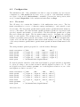
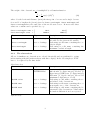
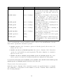
Ocean Assimilation Kit (OAK)
User guide
Alexander Barth, Luc Vandenbulcke
April 9, 2014
1
Structure of the software
The software is structured in different modules
• ufileformat: Binary output and input of large 1D, 2D or 3D matrices in the
GHER or NetCDF.
• initfile: Input of integers, floating numbers, strings and small vectors of those
data types.
• matoper: Basic matrix operating: multiplication, matrix inversion, eigenvalue/eigenvectors
and singular value decomposition (relying on BLAS and LAPACK).
• date: module for conversion between modified Julian day number and Gregorian
date.
• grids: interpolation from one grid to another of 1D, 2D or 3D data.
• rrsqrt: The analysis equation
• assimilation: I/O of state vector, observations, error space and observation operator. Analysis routine with input/output and computation of diagnostics.
These modules can be either used for specific task with standalone programs 5 or by a
hydrodynamic model in the case of a simulation assimilating observations. The GHER
hydrodynamic model drives the data assimilation modules trough the following subroutines:
• dainit: initialises of the data assimilation modules
• daobs: loads of the next observation to assimilate
• daanalysis: performs the analysis
• damoderr: propagates the error covariance of the model
1
2
Module: ufileformat
This module is used for binary output and input of large 1D, 2D or 3D matrices. The
GHER and a subset of the NetCDF format is currently supported. The matrix can contain
exclusion points (“holes”). Matrices A where the elements are a linear combination of
the indices can also be efficiently represented:
A(i, j, k) = a0 + a1 i + a2 j + a3 k
(1)
Only the coefficient a0 , a0 , a0 and a4 are stored. These file are called degenerated. For
example, the longitude and latitude of each grid point can often be expressed in this way.
For the GHER format, each file represent a real matrix. If the file names ends with .gz,
then the file is uncompressed (with gunzip) in the user’s temporary directory defined
by the environment variable $TMPDIR (or by default in /tmp). Simple Fortran 90-style
extraction can also by performed with the module ufileformat. A coma separated list
of indices or ranges of indices in parenthesis can be appended to the file name, if only a
subsection of the matrix should be loaded.
For example if the file toto.TEM is a 10 x 10 x 10 matrix, the “file”:
toto.TEM(:,:,6) is 10x10x1 matrix containing all elements with the 3rd indices equal
to 6.
toto.TEM(:,end,:) is 10x1x10 matrix containing all elements with the 2nd indices equal
to 10.
toto.TEM(1:,:end,1:end) is 10x10x10 matrix equal to the original matrix
But no arithmetic with the indices (for example toto.TEM(:,end-1,:)) are allowed. If
data extraction is used with degenerated matrices, the four coefficient are changed accordingly to the subsection chosen.
Data extraction and automatic decompression can only be used for loading data.
A variable in a NetCDF file can be loaded by specifying a “file name” of the following
form:
NetCDF_filename#NetCDF_variable
If the NetCDF file name end with .gz, then the file is uncompressed as with the GHER
file format. The data extraction follows also the same rules as above. For example, the
following is a valid file name for loading a matrix.
file.nc.gz#temp(:,:,1)
The file file.nc.gz is first decompressed, then the slice with the 3rd indices equal to 1
of the variable temp is returned to the calling program.
The special value for missing data is stored in the variables attribute missing data. In
the case of degenerated file, the attribute shape must be present, containing the shape
of the matrix. The actual value of the variable contains the coefficients ai .
2
2.1
Order of the dimensions
The reported order of the dimensions depends on the tool that you are using to query
and access a file. Two types of ordering schemes exists:
column-major order : used by Fortran programs such as OAK
row-major order : used by C programs such as ncdump
The order of the dimensions for NetCDF follows the recommendation of the CF-convention.
If you query your NetCDF files with ncdump, the order of the dimensions should be time,
depth, latitude, longitude. For a Fortran program reading this file the dimensions with
automatically be longitude, latitude, depth and time since Fortran uses the column-major
order (as opposed to ncdump). For Fortran binary files, the order of the dimensions is
also longitude, latitude, depth and time.
3
The initialisation file
With the module initfile a program can read an integer number, floating number or
a character string from an initialisation file. Each line in this file is composed by a name
(called key), an equal sign and the value. For example:
runtype = 2
Geoflow.maxU = 0.3
logfile = ’assim.log’
When the program search for example the key “runtype”, it gets the integer 2. If a key
is present several times in the same initialisation file, then the last value found is taken.
The key can be composed by any alphanumeric character and by periods (.). In particular, spaces and a equal signs are not allowed within the key name. The wild cards
symbols *, ? and brackets ([,]), are allowed but have a special meaning (see Paragraph
below).
Vectors of integers, floats and character strings are also supported. The values are separated with commas and enclosed in brackets.
Model.variables = [’ETA’,’TEM’,’SAL’]
Model.maxCorrection = [0.3,3.,2.,0.3,3.,2.,0.3,3.,2.]
Blank lines are ignored and comments begin with the pound sign (#). It is recommended
to document the meaning and the possible values by a comments directly in the initialisation file.
Entries in this files cannot be split across different lines. Before assigning a value to a
key you should know with type is expected: scalar or vector and number or characters.
If the type does not correspond, the program will be stopped.
Sometimes a sequence of keys are attributed to the same values:
3
Obs001.path
Obs002.path
Obs003.path
= ’/u/abarth/soft/Ligur3/Obs/’
= ’/u/abarth/soft/Ligur3/Obs/’
= ’/u/abarth/soft/Ligur3/Obs/’
In this case one can use wild cards and write the following:
Obs*.path
= ’/u/abarth/soft/Ligur3/Obs/’
The meaning of the wild cards are the same as for file name generation of the Burne Shell
(see also man page of sh and gmatch).
4
4.1
Assimilation module
Reduced order analysis
Let N be the ensemble size, n the size of the state vector and m the observation space dimension. The best linear unbiased estimator (BLUE) of the model’s state vector given the
model forecast xf with error covariance Pf and the observation yo with error covariance
R is given by xa :
xa = xf + K yo − Hxf
K = Pf HT HPf HT + R
(2)
−1
Pa = Pf − KHPf
(3)
(4)
where H is the observation operator extracting the observed part of the state vector and
Pa the error covariance of the analysis xa .
(k)
From the ensemble of forecast states xf
where k = 1, . . . , N one can compute the
ensemble mean
xf =
N
1 X f (k)
x
N k=1
(5)
and ensemble covariance:
N
(k)
T
1 X f (k)
x
− xf xf − xf
P =
N − 1 k=1
f
(6)
We construct the columns of the matrix Sf by:
(k)
f
S
k
xf − xf
= √
N −1
(7)
where Sf is a n×N matrix, which each column being the difference between each member
its ensemble mean. Its mean over all columns it thus zero. As many other assimilation
schemes (SEEK, RRSQRT, ESSE, EnKF), Pf is decomposed in terms of this square root
matrix Sf :
T
Pf = Sf Sf
(8)
4
Typically, the number of ensemble members N is much smaller than the state vector size
n. We rewrite the Kalman Filter analysis, by avoiding any matrix of the size n × n:
h
i−1
T
T
K = (Sf Sf )HT H(Sf Sf )HT + R
−1
= Sf (HSf )T HSf (HSf )T + R
−1
(HSf )T R−1
= Sf I + (HSf )T R−1 HSf
(9)
(10)
(11)
Where the Sherman-Morison-Woodbury identity has been applied from (10) to (11). This
identity can be expressed as:
ABT C + BABT
−1
−1
= A−1 + BT C−1 B BT C−1
(12)
with A = I, B = HSf , C = R. That is, instead of performing the inverse in space of
matrix A the inverse is done in the space of the matrix C. We also substitute Pf in the
expression of the analysis covariance error Pa :
Pa = Pf − KHPf
f
fT
f
fT
(13)
f
fT
− KHS S
−1
T
= S S − Sf I + (HSf )T R−1 HSf
(HSf )T R−1 HSSf
h
i T
−1
= Sf I − I + (HSf )T R−1 HSf
(HSf )T R−1 HS Sf
= S S
(14)
(15)
(16)
In order to avoid to form Pa explicitly, we need to express Pa also in terms of the square
root matrices Sa .
Pa = Sa SaT
(17)
This is possible when the following eigenvalue decomposition is made :
HSf
T
R−1 HSf = UΛUT
(18)
where UT U = I and where Λ is diagonal. U and Λ are both of the size N × N .
Using the decomposition (18) in equation (16) one obtains:
T
Pa = Sf I − (I + UΛUT )−1 UΛUT Sf
T
= Sf I − (I + UΛUT )−1 UΛUT + I − I Sf
T
= Sf I − (I + UΛUT )−1 UΛUT + I + (I + UΛUT )−1 Sf
T
= Sf I − I + (I + UΛUT )−1 Sf
= Sf (I + UΛUT )−1 Sf
f
T
= S (UU + UΛU ) S
f
−1
f
−1/2
T
(I + Λ)
(21)
(22)
(24)
fT
= S U(I + Λ) U S
= S U(I + Λ)
(20)
(23)
T −1 f T
T
(19)
(25)
−1/2
5
T
U S
fT
(26)
So we found a square root decomposition of Pa in terms of Sf U(I + Λ)−1/2 . But in order
to construct an ensemble from the columns of Sa , its mean has to be zero. So we will
transform Sa so that the identity (26) is preserved. One way to do this is
Sa = Sf U(I + Λ)−1/2 UT Ω
(27)
The decomposition (18) can also be used in the computation of the Kalman gain K: by:
−1
(HSf )T R−1
K = Sf I + (HSf )T R−1 HSf
−1
= Sf UUT + UΛUT
(HSf )T R−1
−1
f
T
f T
= S U(I + Λ) U (HS ) R
(28)
(29)
−1
(30)
a
Ω is an orthogonal matrix chosen such that sum of all columns of S is zero. This sum
can be obtained by multiplying to the right with a vector N × 1 with all elements equal
to 1 (IN ×1 ). Since Sf IN ×1 is zero, Sa IN ×1 is also zero if:
U(I + Λ)−1/2 UT Ω IN ×1 = IN ×1
Ω IN ×1 = U(I + Λ)1/2 UT IN ×1
(31)
(32)
We defined the normalised vectors w and v:
1
w = √ IN ×1
N
v = αU(I + Λ)−1/2 UT IN ×1
(33)
(34)
Ω is thus a matrix which rotates w onto v.
Ωw = v
(35)
It can be computed by:
Ω = vwT + H(v)H(w)T
(36)
where H(v) is the N × (N − 1) Householder matrix associated to the vector v, i.e. all
columns of H(v) are vectors perpendicular to v (Hoteit et al., 2002):
vi vj
for i ≤ N − 1
|vN | + 1
(vN + sgn(vN ))vj
= −
|vN | + 1
H(v)i,j = δi,j −
H(v)N,j
(37)
(38)
Sa is the square root of Pa :
Pa = Sa SaT
a
(39)
a
Based on x and S , an ensemble can be reconstructed:
xa(k) = xa +
√
N − 1 Sa(k)
(40)
The bias aware analysis scheme of Dee and Silva (1998) is also implemented. But the
error space Sa is not computed.
6
4.2
Configuration
The initialisation file of the assimilation module is composed mainly by four sections:
configuration of the model (model state vector, position of the individual variables,
error space of the model), observations to assimilate (observations, their position, their
error), eventual diagnostics of the analysis and miscellaneous flags.
4.2.1
The model
The following code contains the definition of the multivariate state vector. The key
Model.variables is a vector of character strings attributing to each variable a user
chosen name. The keys Model.gridX, Model.gridY, Model.gridZ and Model.mask are
vectors of file names. The files in Model.gridX and Model.gridY are degenerated and
give the longitude and latitude of each variable. The files in Model.gridZ can be plain
files and contains the depth. The key Model.mask is used to determine the sea-land
mask of each variable. The exclusion value (or missing value or FillValue in NetCDF
terminology) marks a land point all other values, a sea points. Every files assembled into
a state vector should have physical values where mask assumes a sea point. The shape
of the arrays in Model.gridX, Model.gridY, Model.gridZ and Model.mask must be the
same.
The string in Model.path in prepended to each file names. Example:
Model.variables
Model.gridX
Model.gridY
Model.gridZ
Model.mask
Model.path
=
=
=
=
=
=
[’ETA’
,’TEM’
,’SAL’]
[’ligur.X(:,:,end)’,’ligur.X’,’ligur.X’]
[’ligur.Y(:,:,end)’,’ligur.Y’,’ligur.Y’]
[’ligur.Z(:,:,end)’,’ligur.Z’,’ligur.Z’]
[’ligur.Z(:,:,end)’,’ligur.Z’,’ligur.Z’]
’/u/abarth/soft/Ligur3/Data/’
For nested grids the variables of the same nested must be grouped and the groups must
be orders according to the resolution started with the highest resolution one. To each
model grid is associated a Model.gridnum: one for the highest resolution one, two of the
next highest resolution one and so one.
Model.variables
Model.gridX
Model.gridY
Model.gridZ
Model.mask
Model.gridnum
Model.path
=
=
=
=
=
=
=
[’TEM’
,’SAL’
,’TEM’,
’SAL’]
[’ligur.X’,’ligur.X’,’med.X’,’med.X’]
[’ligur.Y’,’ligur.Y’,’med.Y’,’med.Y’]
[’ligur.Z’,’ligur.Z’,’med.Z’,’med.Z’]
[’ligur.Z’,’ligur.Z’,’med.Z’,’med.Z’]
[
1,
1,
2,
2]
’/u/abarth/soft/Ligur3/Data/’
Mandatory keys
7
Key
ErrorSpace.dimension
ErrorSpace.init
Type
integer
vector of strings
Description
The dimension of the error space.
Each string is a Fortran format containing an
integer descriptor. The format is converted
into a file name with an internal write. The
integer is a number ranging from 1 to the dimension of the error space n. n vectors of file
names are formed and represent a error mode
in the state space. Their norm represent the
importance of the error mode and thus they
are in general not normed. Orthogonality is
not necessary.
Key
ErrorSpace.path
Type
string
ErrorSpace.scale
real
ErrorSpace.spaceScale
vector of strings
Description
The path is prepended to all file names specified in ErrorSpace.*. The current path is
used by default.
Each error mode is multiplied by this real
number. The default is 1.
Each error mode is multiplied element by element by this vector. The default is a vector
with all elements equal to 1.
Optional keys
4.2.2
Zones
When the local version of the assimilation algorithm (schemetype = 1) is used, then
the assimilation is performed in a number of zones independently. Zones are defined by
specifying a partition vector which has the same number of variables as the model state
vector and each variable has the same size as the corresponding Model.mask. This vector
contains only integer values starting with one and represent labels: all elements in the
state vector which have the same partition number belong to the same zone. For example,
for a state vector with 5 elements and the partition vector p:


 
x1
1
 1 
 x2 

 


 2 
x
p
=
(41)
x=
3

 

 x4 
 2 
x5
3
This partition vector defined three zones: the first zone contains elements x1 and x2 , the
second zone x3 and x4 and the third zone x3 . There should be no gaps in the partition
vector. For example the vector (1, 1, 2, 2, 4)T would cause an error. In practice, the state
vector is partitioned along water columns. The assimilation is performed independently
in each zone using only observations within the search radius given by Zones.maxLength.
8
The weight of the observations
1
R0
is multiplied by a Gaussian function:
1
1
= 0 exp(−(d/L)2 )
0
R
R
(42)
where d is the horizontal distance (in m) the first point of a zone and a single observation and L a length-scale (in m) given by Zones.corrLength. Zones.maxLength and
Zones.corrLength have the same size as the model state vector. In most cases these
values are constant can be specified by, e.g.:
Zones.corrLength.const = [
Zones.maxLength.const = [
30e3,
2000e3,
Key
Zones.partition
Type
vector of strings
Zones.corrLength
vector of strings
Zones.maxLength
vector of strings
4.2.3
30e3]
2000e3]
Description
Each string is a file name containing the partition file for the given model variable
Each string is a file name containing the correlation length
Each string is a file name containing the
maximum correlation length
The observations
All set of simultaneous observation are ordered chronically and are attributed to a time
index starting with 001 (written always with three digits). In the following keys “XXX”
have to be replaced by the time index.
Mandatory keys
Key
ObsXXX.time
Type
’yyyy-mmddTHH:MM:ss’
ObsXXX.value
vector of strings
ObsXXX.rmse
vector of strings
ObsXXX.mask
vector of strings
Optional keys
9
Description
yyyy=year (minimum 1 digit integer)
mm=month (2 digits integer) dd=day (2
digits integer) HH=hour (2 digits integer)
MM=min (2 dig-ids integer) SS=second
(minimum 1 digit integer or real)
Each string is a file name containing the actual values of the observations
Each string is a file name containing the root
mean square error of the observations.
Each string is a file name containing the binary mask of the observations. Values where
the mask is different from 1 are rejected.
Key
ObsXXX.variables
Type
vector of strings
Description
The names must correspond to the names
chosen in Model.variables. Unknown names
are treated as ”out of the grid” and are not
assimilated.
ObsXXX.names
vector of strings
Each string is a description of the data type
of the observations. You can choose any
name meaningful to you. These names are
only used for the log-file. The default names
are Var01, Var02,...
ObsXXX.gridX
vector of strings
Each string is a file name containing the longitude of the observations.
ObsXXX.gridY
vector of strings
Each string is a file name containing the latitude of the observations.
ObsXXX.gridZ
vector of strings
Each string is a file name containing the
depth of the observations.
ObsXXX.HperObs
vector of strings
The observation operator stored in a sparse
matrix form per observations
ObsXXX.operator
string
The observation operator stored in a sparse
matrix form.
ObsXXX.path
string
The path is prepended to all file names specified in ObsXXX.*. The current path is used
by default.
The optional keys are used to create the observation operator. If it is applied to the state
vector, it extracts the observed variables at the location of the measurements. Several
ways exist to specify the observation operator.
1. ObsXXX.operator: the observation operator is directly given by the non zero elements. See also 4.2.3.
2. ObsXXX.variables and ObsXXX.HperObs: the non zero elements of the observation
operator for each variable are given separately. The first column in 9 × x matrix is
ignored. See also 4.2.3.
3. ObsXXX.variables, ObsXXX.gridX, ObsXXX.gridY and ObsXXX.gridZ: the observation operator is created by a trilinear interpolation using the module grids.
Note that the individual arrays in ObsXXX.value, ObsXXX.rmse, ObsXXX.mask, ObsXXX.gridX,
ObsXXX.gridY and ObsXXX.gridZ should have the same size.
Format of the observation operator
Only the non-zero elements of the observation operator are specified in the 9 × n matrix
(in column-major order) where n is the number of non-zero elements. Each column has
the following structure:
10
var. index
Observations
i-index j-index
k-index
var. index
Model
i-index j-index
k-index
Interpolation
coefficient
The first integer value is related to the observation. The index of the variable is the
position where the observed variable appears in ObsXXX.value and i,j,k-index are the
three spatial indexes of a single scalar observation.
The integers in column 5 to 8 are related to the model state vector. Again the index
of the variable is the position where the observed variable appears in Model.variables
and i,j,k-index are the three spatial indexes of a single scalar model forecast. If one of
the model indexes is -1 the corresponding observation is treated ”out of grid” and the
associated weight will be zero.
The column 9 is a real value between 0 and 1 in the case of a simple trilinear interpolation.
The observation operator can be generated offline using a trilinear interpolation with the
tool ”genobsoper”.
4.2.4
Diagnostics
All diagnostics are optional and the corresponding files are output.
11
Key
DiagXXX.xf
DiagXXX.Hxf
DiagXXX.Sf
Type
vector of strings
vector of strings
vector of strings
DiagXXX.Ef
vector of strings
DiagXXX.diagPf
vector of strings
DiagXXX.diagHPfHT
vector of strings
DiagXXX.stddevxf
vector of strings
DiagXXX.stddevHxf
vector of strings
DiagXXX.path
string
DiagXXX.xa
DiagXXX.Hxa
DiagXXX.Sa
vector of strings
vector of strings
vector of strings
DiagXXX.Ea
vector of strings
DiagXXX.diagPa
vector string
DiagXXX.diagHPaHT
vector of strings
DiagXXX.stddevxa
vector of strings
DiagXXX.stddevHxa
vector of strings
DiagXXX.H
DiagXXX.yo
DiagXXX.invsqrtR
strings
vector of strings
vector of strings
DiagXXX.xa-xf
DiagXXX.yo-Hxf
vector of strings
vector of strings
12
DiagXXX.yo-Hxa
vector of strings
DiagXXX.Hxa-Hxf
DiagXXX.path
vector of strings
string
Description
the model forecast (ensemble mean)
the observed part of the model forecast
Each string is a Fortran format.
For
the conversion into file names see the key
ErrorSpace.init. The files represent the
error modes of the model forecast.
Each string is a Fortran format.
For
the conversion into file names see the key
ErrorSpace.init. The files represent the
forecast ensemble.
The diagonal elements of error covariance of
the model forecast.
The diagonal elements of error covariance of
the observed part of the model forecast
Standard deviation of the error of the model
forecast.
Standard deviation of the error of the observed part of the model forecast.
The path is prepended to all file names specified in DiagXXX.*. The current path is used
by default.
the analysis (ensemble mean)
the observed part of the analysis
Each string is a Fortran format.
For
the conversion into filenames see the key
ErrorSpace.init. The files represent the
error modes of the analysis.
Each string is a Fortran format.
For
the conversion into file names see the key
ErrorSpace.init. The files represent the
analysis ensemble.
The diagonal elements of error covariance of
the analysis.
The diagonal elements of error covariance of
the observed part of the analysis
Standard deviation of the error of the analysis.
Standard deviation of the error of the observed part of the analysis.
the observation operator
The observations.
The inverse of the root mean square error
of the observations. If a scalar observation
point has been eliminated (out of the model
grid for example) its weight is zero.
The analysis increment
the observation minus the model forecast at
the observation points
the observation minus the model analysis at
the observation points
analysis increment at the observation points
The path is prepended to all filenames spec-
4.2.5
miscellaneous flags
Key
nbnest
assimnum
Type
integer
integer
runtype
integer
Description
Number of nested grids
Number between 1 and nbnest different for
each model. The model with assimnum does
the assimilation
possible values of runtype are:
0: do nothing, i.e. a pure run of the model
1: still do not assimilate, but compare model
to observations
2: assimilate observations
schemetype
integer
possible values of schemetype are:
0: global assimilation (default)
1: local assimilation (Zones need to be defined)
moderrtype
integer
possible values of moderrtype are:
0: optimal interpolation Pf constant
1: forgetting factor approximation
biastype
integer
possible values of biastype are:
0: standard bias-blind analysis
1: A fraction of the error (gamma) is a systematic error and the rest (1-gamma)
is random (Dee and Silva, 1998)
Bias.gamma
Bias.init
joinvectors
real
vector of string
integer
logfile
string
debugfile
string
13
fraction of the error with is systematic
the initial estimation of the bias
If joinvectors is 1 then the variables of the
nested grids will be assembled to one multigrid state vector
File contains simple diagnostics such as rmse
with observations
File contains debugging information is the
code was compiled with the flag -DDEBUG
5
5.1
Standalone programs
Program assim
The standalone program assim can be used to test the assimilation. The program can
be called from the command line:
assim <initfile> <time index>
The first argument is the initialisation file and the second argument is the time index of
the observation to assimilate. All keys described in 4.2 have the same meaning for the
program assim. But the forecast has to be specified by the following keys.
Key
Type
Description
ForecastXXX.value
vector of strings
the forecast
ForecastXXX.path
string
The path is prepended to all filenames specified in ForecastXXX.value. The current
path is used by default.
If the program is called with three arguments:
assim <initfile> <start time index>
<end time index>
All assimilation cycles be between the two time indexes are performed in chronological
order.
5.2
Program genobsoper
The standalone program genobsoper generate the observation matrix.
genobsoper <initfile> <time index>
The first argument is the initialisation file and the second argument is the time index of
the observation for witch the observation operator has to be created. All keys described
in 4.2 have the same meaning for the program genobsoper. But the only diagnostic key
used is DiagXXX.H.
If the program is called with three arguments:
genobsoper <initfile> <start time index>
<end time index>
The action is repeated for all time indexes between the start and the end time index.
5.3
Program applyobsoper
The standalone program applyobsoper extracts from a state vector the observations.
applyobsoper <initfile> <time index>
14
The first argument is the initialisation file and the second argument is the time index of
the observation for witch the observation operator has to be created. All keys described
in 4.2 have the same meaning for the program applyobsoper. But the only diagnostic
key used are DiagXXX.Hxf and DiagXXX.invsqrtR. If a scalar observation point has been
eliminated (out of the model grid for example) its weight in DiagXXX.invsqrtR is zero.
The state vector is specified as it is described in 5.1.
If the program is called with three arguments:
applyobsoper <initfile> <start time index>
<end time index>
The action is repeated for all time indexes between the start and end time index.
5.4
Program filteroper
The standalone program filteroper generates a sparse matrix witch acts as a spatial
filter in the model space.
filteroper <initfile>
For each variable the filter is a Gaussian function:
0
0
0
f (x, y, z, x , y , z ) = N e
−
(y−y 0 )2
(z−z 0 )2
(x−x0 )2
−
−
L2
L2
L2
x
y
z
(43)
N is a normalisation factor taking in to account the land-sea mask. The parameters Lx ,
Ly and Lz may be space dependent and have thus the same dimension as the state vector.
The required keys are:
Key
Model.mask
Model.gridX
Model.gridY
Model.gridZ
Model.path
Type
vector
vector
vector
vector
string
Correlation.lenx
Correlation.leny
Correlation.lenz
Correlation.path
vector of strings
vector of strings
vector of strings
string
Filter
string
5.5
of
of
of
of
strings
strings
strings
strings
Description
sea-land mask of each variable
longitude of each variable (degenerated file)
latitude of each variable (degenerated file)
depth
The path is prepended to all filenames specified in Model.*. The current path is used
by default.
parameter Lx in equation 43
parameter Ly in equation 43
parameter Lz in equation 43
The path is prepended to all filenames specified in Correlation.*. The current path is
used by default.
file name of the filter
Program opermul
opermul is a general purpose program witch multiply two sparse operators. It can be
used for example for multiplying a filter operator and a observation operator.
O3 = O2 O1
15
(44)
O1 is a operator mapping from space S1 to S2 , O2 from S2 to S3 and thus the product
from S1 to S3 .
opermul <initfile>
The required keys are:
Key
Space1.mask
Space1.path
Type
vector of strings
string
Space2.mask
Space2.path
vector of strings
string
Space3.mask
Space3.path
vector of strings
string
Term1
Term2
Product
string
string
string
5.6
Description
sea-land mask of space S1
The path is prepended to all filenames specified in Space1.mask. The current path is
used by default.
sea-land mask of space S1
The path is prepended to all filenames specified in Space2.mask. The current path is
used by default.
sea-land mask of space S1
The path is prepended to all filenames specified in Space2.mask. The current path is
used by default.
file name of operator O1
file name of operator O2
file name of the product O3
Matlab utility GenObsFile
The utility ”GenObsFile” provides an easy way to save all the observations, coming from
various sources, in a few files with the NetCDF format, and creates the .INIT file required
by the assimilation routines.
Options for GenObsFile must be specified in the header of the Matlab routine, as described below:
• initheader: complete path & file name, of the file that must be copied on top of the
.INIT file. This could be the ”model” part of the .INIT file.
• diags: complete path & file of a sample ”diagnostic” part of the .INIT file. The
observation number should be replaced with <INDEX> and variable names with
<EXT>. This part will be (adapted and) copied for each observation set.
Example:
Diag<INDEX>.Hxf =
[’xf.<EXT>’]
• Outdir : path where to store the new observations and .INIT file.
• Outfile : prefix of the new observation files
• maxX, minX, maxY, ..., minMJD: observations not within these ranges will be
ignored when creating the new observation files
16
• rmse : vector containing errors on the observations, in the following order:
[TEM SAL ETA other]=[...]
It will only be used by the assimilation routine if no other observation error covariance R matrix is specified. GenObsFile only uses values corresponding to variables
present in your observations list.
• obstime : time of the day at which observations should be assimilated
• listfile : complete path+file name for the listfile, which contains the original observations. It is build using sections. There must be at least one section in the
listfile. Each section contains a ”config” line followed by an arbitrary amount of
data lines. The config line starts with the keyword ’config’, and has the following
format: config VAR X Y Z MJD
– VAR indicates how the observed data should be named in the .INIT file (TEM
...)
– X might be (a) a complete path+file name with the longitude data, corresponding to the observations, (b) the keyword ’file’ if the longitude data is
written in a file with the same file name as the actual data, with extension .X
– Y (idem)
– Z (idem)
– MJD points to the file containing the MJD-time corresponding to the
– observations, and might be (a) a complete path+file name, (b) the
– keyword ’file’, (c) a datum in the format 1999-12-31, (d) a datum in
– the MJD format ’51251’, (e) character limits to be found in the
– actual observations file name.
For example, if the actual file name is /home/johndoe/51657.TEM , MJD could
be 15-19 as those are the indexes pointing to 51657 in the file name. After each
config line, an arbitrary amount of observation files may be given. The filenames
may contain matrix delimiters, as in (1:100,2:5,:)
Example listfile:
17
config TEM ./Lion.X ./Lion.Y ./Lion.Z 1998-01-01
/home/johndoe/observations/Lion00000480.TEM.gz(:,:,end)
config SAL ./Lion.X ./Lion.Y ./Lion.Z 1998-01-01
/home/johndoe/observations/Lion00000480.SAL.gz(:,:,end)
config TEM file file file file
/home/johndoe/observations/ctd02.1_03_aug_2241.TEM
/home/johndoe/observations/ctd03.1_03_aug_1840.TEM
/home/johndoe/observations/ctd04.1_04_aug_0747.TEM
config TEM ./ligur.SST.X ./ligur.SST.Y ./ligur.SST.Z 32-41
/scratch/johndoe/observtn/ligur1999-07-02.SST.gz
/scratch/johndoe/observtn/ligur1999-07-03.SST.gz
/scratch/johndoe/observtn/ligur1999-07-04.SST.gz
/scratch/johndoe/observtn/ligur1999-07-10.SST.gz
/scratch/johndoe/observtn/ligur1999-07-11.SST.gz
6
6.1
API
ufileformat
uload(filename,matrix,exclusion value)
filename : character of strings, input. The filename of the matrix to load with
the extensions described in 2.
matrix : 1D, 2D or 3D unallocated real pointer, output. The allocation of the
output matrix is done inside the subroutine.
exclusion value : real, output: The exclusion value
usave(filename,matrix,exclusion value)
filename : character of strings, input. The filename of the matrix to save.
matrix : 1D, 2D or 3D real matrix, input. The matrix to save.
exclusion value : real, input: The exclusion value
References
D. P. Dee and A. Silva. Data assimilation in the presence of forecast bias. Quarterly
Journal of the Royal Meteorological Society, 124:269–295, 1998.
I. Hoteit, D.-T. Pham, and J. Blum. A simplified reduced order Kalman filtering and application to altimetric data assimilation in Tropical Pacific. Journal of Marine Systems,
36:101–127, 2002.
18