Download KSC-ICD Package User's Manual - Esat

KSC-ICD Package User’s Manual
Fast kernel spectral clustering based on incomplete
Cholesky factorization for large scale data analysis
Authors
´ ly Nova
´k
Miha
Institute for Nuclear Research of the Hungarian Academy of Sciences
MTA-ATOMKI
Debrecen, Hungary
Carlos Alzate
Smarter Cities Technology Centre
IBM Research
Dublin, Ireland
Rocco Langone and Johan A.K. Suykens
Katholieke Universiteit Leuven
ESAT-STADIUS
Leuven, Belgium
2014
Acknowledgement
The research leading to these results has received funding from the European Research Council under the European Union’s Seventh Framework Programme (FP7/2007-2013) / ERC AdG A-DATADRIVE-B (290923). This
paper reflects only the authors’ views, the Union is not liable for any use
that may be made of the contained information. Research Council KUL:
GOA/10/09 MaNet, CoE PFV/10/002 (OPTEC), BIL12/11T; PhD/Postdoc grants Flemish Government: FWO: projects: G.0377.12 (Structured
systems), G.088114N (Tensor based data similarity); PhD/Postdoc grants
IWT: projects: SBO POM (100031); PhD/Postdoc grants iMinds Medical
Information Technologies SBO 2014 Belgian Federal Science Policy Office:
IUAP P7/19 (DYSCO, Dynamical systems, control and optimization, 20122017)
Contents
1 Introduction
5
2 Installation
7
3 Demo executables
3.1 Incomplete Cholesky decomposition
3.2 Model selection . . . . . . . . . . .
3.3 Training the sparse KSC model . .
3.4 Out-of-sample extension . . . . . .
4 Example
4.1 Image
4.1.1
4.1.2
4.1.3
4.1.4
4.1.5
5 List
5.1
5.2
5.3
5.4
5.5
.
.
.
.
.
.
.
.
.
.
.
.
.
.
.
.
.
.
.
.
.
.
.
.
.
.
.
.
.
.
.
.
.
.
.
.
.
.
.
.
.
.
.
.
.
.
.
.
11
14
16
20
23
segmentation . . . . . . . . . . . . .
The IMG BID 145086 Q8 data set .
Incomplete Cholesky decomposition
Tuning . . . . . . . . . . . . . . . .
Training . . . . . . . . . . . . . . .
Out-of-sample extension . . . . . .
.
.
.
.
.
.
.
.
.
.
.
.
.
.
.
.
.
.
.
.
.
.
.
.
.
.
.
.
.
.
.
.
.
.
.
.
.
.
.
.
.
.
.
.
.
.
.
.
.
.
.
.
.
.
.
.
.
.
.
.
.
.
.
.
.
.
27
27
27
29
29
30
31
.
.
.
.
.
.
.
.
.
.
.
.
.
.
.
.
.
.
.
.
.
.
.
.
.
.
.
.
.
.
.
.
.
.
.
.
.
.
.
.
.
.
.
.
.
.
.
.
.
.
.
.
.
.
.
35
38
40
43
46
50
of functions
ichol . . . . . . . . . . . . . .
kscWkpcaIchol train . . . . .
kscWkpcaIchol test . . . . . .
kscWkpcaIchol tune . . . . . .
doClusteringAndCalcQuality
3
.
.
.
.
.
.
.
.
.
.
.
.
.
.
.
.
.
.
.
.
.
.
.
.
.
.
.
.
.
.
.
.
.
.
.
.
.
.
.
.
.
.
Chapter 1
Introduction
The kscicd package contains the C implementation of the fast Kernel Spectral Clustering (KSC) algorithm presented in [1]. The algorithm provides a
sparse KSC model with out-of-sample extension and model selection capabilities with a training stage time complexity that is linear in the training
set size. The present algorithm is an improved version of that published
in [2] which has a computational time complexity of the training stage that
is quadratic in the training set size. This prevented the application of the
original sparse KSC model to large scale problems. This quadratic time
complexity has been reduced to linear by the present algorithm while all
the attractive properties of the original algorithm (like simple out-of-sample
extension or simple model selection) remained unchanged.
The KSC problem is formulated as Weighted Kernel PCA [3] in the context of Least Squares Support Vector Machines (LS-SVM) by using primaldual optimization framework [4]. The sparsity is achieved by combining the
reduced set method [5] and the Incomplete Cholesky Decomposition (ICD) [6,
7] of the training set kernel matrix. More details can be found in the references cited above.
The C implementation of the KSC algorithm proposed in [1], given in the
kscicd package, is based on LAPACK [8] and BLAS [9, 10] libraries. The results,
presented in this manual, were obtained by using Fedora 12 operating system
running on an Intel Core 2 Duo, 2.26 GHz, 3.8 GB RAM hardware with an
automatically tuned BLAS library using the freely available ATLAS [11, 12].
Only a single core was used for the computations.
Main developer:
Mih´aly Nov´ak, email: mihaly.novak at gmail.com
The main references to this work are
5
M. Nov´ak, C. Alzate, R. Langone, J.A.K. Suykens, Fast kernel spectral
clustering based on incomplete Cholesky factorization for large scale data
analysis, submitted
M. Nov´ak, C. Alzate, R. Langone, J.A.K. Suykens, Fast kernel spectral
clustering based on incomplete Cholesky factorization for large scale data
analysis, Internal Report 14-119, ESAT-SISTA, KU Leuven (Leuven, Belgium), (2014)
M. Nov´ak, C. Alzate, R. Langone, J.A.K. Suykens, KSC-ICD package user’s
manual, Internal Report 14-120, ESAT-SISTA, KU Leuven (Leuven, Belgium), (2014)
The KSC-IDC package home page is
http://esca.atomki.hu/~novmis/kscicd
Copyright (C) 2014 Mih´
aly Nov´
ak, email: mihaly.novak at gmail.com
This program is free software: you can redistribute it and/or modify it under
the terms of the GNU General Public License as published by the Free Software Foundation, either version 3 of the License, or (at your option) any
later version.
This program is distributed in the hope that it will be useful, but WITHOUT
ANY WARRANTY; without even the implied warranty of MERCHANTABILITY or FITNESS FOR A PARTICULAR PURPOSE. See the GNU General
Public License for more details (http://www.gnu.org/licenses/).
This program is available for non-commercial research purposes only. Notwithstanding any provision of the GNU General Public License, the software may
not be used for commercial purposes without explicit written permission.
Chapter 2
Installation
Installation of the kscicd package builds the kscicd library and some
demo executables. Then you can perform clustering on your own data
without writing any single line of codes by using the demo executables or
you can call the functions of the kscicd library in your own C, C++ applications.
You can build the kscicd package by a single make command on your Linux
system. So you are just a few seconds away from clustering your own data
by means of the kscicd package if you are reading this line.
Step 0.: dependences
The kscicd C library is based on the BLAS and LAPACK libraries. It
means that some of the C functions will call LAPACK and BLAS routines.
So when you link your application with the kscicd library you also need
to link the lapack and blas libraries. Furthermore, when applications are
developed based on LAPACK and BLAS the lapack-devel and blas-devel
libraries are also necessary. So make sure that these libraries are available
on your machine before you start to build the kscicd library and the demo
executables. All these libraries are available in standard repositories so you
can use the command that you usually use to obtain packages (yum, apt-get,
etc.) and type (I use yum on Fedora)
[root@tecra ~]# yum install lapack-devel
Make sure that all the necessary libraries (lapack, lapack-devel, blas, and
blas-devel) are available on your system.
7
Step 1.: obtain the source
The kscicd package as well as some demo data are available on the kscicd
homepage http://esca.atomki.hu/~novmis/kscicd. Go to the directory
where you want to store the kscicd package, download kscicd_package.tar.
gz into that directory and uncompress it. I will use the progs directory on
my system. So first cd into your directory:
[root@tecra ~]# cd progs
[root@tecra progs]#
then download kscicd_package.tar.gz
[root@tecra progs]# wget http://esca.atomki.hu/~novmis/kscicd/
html/downloads/kscicd_package.tar.gz
...
...
...
then uncompress it
[root@tecra progs]# tar -zxvf kscicd_package.tar.gz
...
...
...
Then you will have the kscicd_package directory
Step 2.: building the library and some executables
The kscicd_package directory contains the makefile, the util and demo
subdirectories. We will use the gcc GNU compiler collection in our makefile. cd into the kscicd_package directory where the makefile is located
and type execute the make command to build the kscicd library and the
demo executables:
[root@tecra progs]# cd kscicd_package
[root@tecra kscicd_package]#
[root@tecra kscicd_package]# make
If everything is fine you should see something like this (of course the full path
/root/progs/kscicd_package/... depends on your directory system):
gcc -Iutil/src -I../include -I. -O2 -c util/src/demo/*.c
cd ./util ; make -f makefile_lib
make[1]: Entering directory ‘/root/progs/kscicd_package/util’
mkdir -p lib
gcc -O2 -c src/*.c
ar rcs lib/libkscicd.a *.o
make[1]: Leaving directory ‘/root/progs/kscicd_package/util’
gcc -O2 -o demo/demo_ichol demo_ichol.o -Lutil/lib
-L../lib -lkscicd -llapack -lblas -lm
gcc -O2 -o demo/demo_kscicd_train demo_kscicd_train.o -Lutil/lib
-L../lib -lkscicd -llapack -lblas -lm
gcc -O2 -o demo/demo_kscicd_test demo_kscicd_test.o -Lutil/lib
-L../lib -lkscicd -llapack -lblas -lm
gcc -O2 -o demo/demo_kscicd_tune demo_kscicd_tune.o -Lutil/lib
-L../lib -lkscicd -llapack -lblas -lm
First the kscicd library i.e. libkscicd.a is created into the util/lib/
subdirectory by calling the util/makefile_lib sub-makefile. Then the
demo executables (demo_ichol, demo_kscicd_train, demo_kscicd_test,
demo_kscicd_tune) are built into the demo subdirectory by linking the demo
applications with the libkscicd kscicd library and the liblapack and
libblas LAPACK and BLAS libraries. You can remove all the unnecessary
object files by executing the make clean command as
[root@tecra kscicd_package]# make clean
rm -rf *.o
cd ./util ; make clean -f makefile_lib
make[1]: Entering directory ‘/root/progs/kscicd_package/util’
rm -rf *.o
make[1]: Leaving directory ‘/root/progs/kscicd_package/util’
Then you are ready to use the demo executables for performing clustering on
your own data or to write your own C, C++ application by calling functions
from the kscicd library.
Chapter 3
Demo executables
Some demo executables are also provided by kscicd package beyond the
kscicd library. The source codes are located in the
kscicd_package/util/src/demo/
subdirectory and the executables are built into the
kscicd_package/demo/
subdirectory during the installation. You can use these demo executables to
perform sparse kernel spectral clustering on your own data after the installation.
The sparse kernel spectral clustering algorithm proposed in [1] has two
main steps: training → train the sparse KSC model on the training set and
test → perform out-of-sample extension i.e. clustering arbitrary input data
points by using the sparse KSC model obtained in the training step. The
algorithm proposed in [1] is based on a low rank approximation of the training set kernel matrix obtained by using incomplete Cholesky decomposition
ICD. This step must be done before the training. Kernel spectral clustering
models, as other machine learning algorithms, depend on some user defined
parameters. In case of KSC these parameters are the number of desired
clusters and the parameter of the kernel function. Different values of these
parameters result in different KSC models. One of the biggest advantage of
the weighted kernel PCA formulated KSC model, proposed in [3], is that the
optimal parameter values can be determined by maximizing a model selection criterion on a validation set. This parameter tuning is optional and not
considered to be part of the training.
The demo executables,
demo_ichol, demo_kscicd_tune, demo_kscicd_train, demo_kscicd_test
11
delivered in the kscicd package, are aimed to perform the different steps of
the KSC algorithm [1] discussed above in order to demonstrate the working
of the kscicd library functions. The codes were kept as simply as possible
(and not necessarily optimal regarding data I/O) in order to make easier to
read. Some temporary data will be stored in the
kscicd_package/demo/demo_data/io/
directory between the different steps of the KSC algorithm i.e. between the
execution of the different demo applications.
Demo data set and kernel function
The demo data set, that will be used in this chapter to demonstrate the working of the demo applications and the corresponding kscicd library functions,
is the G10_N1M data set that is available on the kscicd homepage http://
esca.atomki.hu/~novmis/kscicd. Go to the kscicd_package/demo/demo
_data/ subdirectory, download the G10_N1M.tar.gz file into this directory
and uncompress it:
[root@tecra kscicd_package]# cd demo/demo_data
[root@tecra demo_data]#
[root@tecra demo_data]# wget http://esca.atomki.hu/~novmis
/kscicd/html/downloads/G10_N1M.tar.gz
...
...
...
[root@tecra demo_data]# tar -zxvf G10_N1M.tar.gz
G10_N1M/
G10_N1M/data_G10_K10_ovl_Valid_40000
G10_N1M/data_G10_K10_ovl_Full_1E6
G10_N1M/data_G10_K10_ovl_Train_20000
The G10_N1M data set contains 106 data points sampled from 10 (slightly
overlapping) 2D Gaussian distributions. Each of the K = 10 cluster contains
105 input data points. The G10_N1M directory contains the following files:
data_G10_K10_ovl_Full_1E6
data_G10_K10_ovl_Train_20000
the full data set with 106 2D data
points
2·104 data points for training; sampled
randomly from the full data set
data_G10_K10_ovl_Valid_40000
4 · 104 data points for validation; the
union of the 2 · 104 size training data
set and 2 · 104 additional data points
sampled randomly from the full data
set
The radial basis function (RBF) kernel will be used in this chapter that is implemented in the kscicd_package/util/src/demo/kscicd_kerns.c source
file that is included into each demo application. (see the notes on the kernel
function implementation at the beginning of chapter 5 for more details).
3.1
Incomplete Cholesky decomposition
This demo application performs the incomplete Cholesky decomposition of
the training set kernel matrix by using the ichol function from the kscicd
library. See section 5.1 for the detailed description of the ichol function.
source code:
kscicd_package/util/src/demo/demo_ichol.c
executable:
kscicd_package/demo/demo_ichol <arg1> <arg2> ... <arg8>
Input parameters:
The corresponding ichol function parameters are indicated in the second
column of the table. See section 5.1 for the detailed description of the ichol
function.
arguments
arg1
arg2
arg3
arg4
arg5
arg6
pars.
N
D
H
*TOL
*R
arg7
arg8
-
description
number of training data points
dimension of training data points
kernel function flag: =0→ RBF kernel, =1→ χ2 kernel
kernel parameter
error tolerance in the ICD algorithm
maximum rank of the approximation i.e. maximum number
of columns that can be selected during the ICD
path to the io directory
path to the training data file
Output:
Will write the incomplete Cholesky factor matrix, the permutation vector
and the permuted training data set into the io directory as separate files
with the names of res_icholfactor, res_pivots and res_trainingdata
respectively.
Application:
The arg1 = 20000 arg2 = 2 2D training data points are stored in the arg8 =
demo_data/G10_N1M/data_G10_K10_ovl_Train_20000 file. We will use the
arg3 = 0 RBF kernel with arg4 = 0.01 kernel parameter. The error tolerance
will be set to arg5 = 0.75 while the maximum rank arg6 = 200. The io directory is located within the demo_data directory so arg7 = demo_data/io/.
So we can execute the demo_ichol application:
[root@tecra demo]# ./demo_ichol 20000 2 0 0.01 0.75 200
demo_data/io/ demo_data/G10_N1M/data_G10_K10_ovl_Train_20000
Time: = 2.92 [s]
Rank: = 158
Tol: = 0.744916
The incomplete Cholesky decomposition (ICD) algorithm terminates after
2.92 seconds because the given tolerance value tol = 0.75 is reached. R =
158 points were selected out of the 20 000 training data points by the ICD
algorithm when the given tolerance is reached.
3.2
Model selection
The demo_kscicd_tune application calculates the values of the chosen model
selection criterion over a cluster number - kernel parameter grid by using the
kscWkpcaIchol_tune function from the kscicd library. It is strongly recommended to examine the whole grid delivered by this application (through
the kscWkpcaIchol_tune function) before the acceptance of the optimal parameter values chosen by the application. See section 5.4 for the detailed
description of the kscWkpcaIchol_tune function.
The incomplete Cholesky factor matrix and the permuted training data are
inputs of the demo _kscicd_tune application. It means that the demo_ichol
application must be executed before using demo_kscicd_tune in order to
ensure that both the res_icholfactor and the res_trainingdata files are
available in the io directory.
source code:
kscicd_package/util/src/demo/demo_kscicd_tune.c
executable:
kscicd_package/demo/demo_kscicd_tune <arg1> <arg2> ... <arg14>
Input parameters:
The corresponding kscWkpcaIchol_tune function parameters are indicated
in the second column of the table. See section 5.4 for the detailed description
of the kscWkpcaIchol_tune function.
arguments
arg1
arg2
arg3
pars.
N
D
R
arg4
arg5
NV
QMF
arg6
ETA
description
number of training data points;
dimension of training data points
number of columns in the incomplete Cholesky factor
obtained previously by using the demo_ichol application (see section 3.1)
number of validation data points
model selection criterion flag (see further notes on QMF
parameter in section 5.2)
this is the η parameter value; the trade-off between the
collinearity measure and balance terms of the selected
model selection criterion
arg7
arg8
arg9
arg10
H_MIN
H_MAX
NH
arg11
arg12
C_MIN
C_MAX
arg13
-
arg14
-
kernel function flag: =0→ RBF kernel, =1→ χ2 kernel
minimum kernel parameter value
maximum kernel parameter value
number of kernel kernel parameter values to test in
[H MIN,H MAX] interval; logarithmic spacing will be
used to generate the kernel parameter values
minimum cluster number value
maximum cluster number value; each value will be
tested in [C MIN,C MAX]
path to the io directory; some results of the incomplete
Cholesky decomposition, (like the incomplete Cholesky
factor matrix, permuted training data set) are stored
in this io directory and will need now
path to the validation data file
Output:
The application will call the kscWkpcaIchol_tune function from the kscicd
library. This function trains the KSC model on the training set at each
cluster number - kernel parameter grid point. The different KSC models,
obtained by training at the different grid points, is used then to perform
out-of-sample extension of the trained models to the validation set. The
chosen model selection criterion is evaluated on the results obtained on the
validation set. The kscWkpcaIchol_tune function delivers the model selection criterion values over the cluster number - kernel parameter grid in
the QM matrix (see further notes in section 5.4 on the structure of the QM).
The demo_kscicd_tune application will write this QM matrix into the current
directory in gnuplot format as a Q_m file. Then you can select the cluster
number, kernel parameter values that corresponds to the most optimal model
by examine the model selection surface over the grid.
Application:
The demo_kscicd_tune application needs the incomplete Cholesky decomposition of the training set kernel matrix and the permuted training data
set. These can be obtained by executing the demo_ichol application (see
section 3.1). So the demo_ichol application must be executed before the
demo_kscicd_tune in order to ensure that the res_icholfactor and res
_trainingdata files are available in the arg13=demo_data/io/ directory.
The res_trainingdata file stores the arg1 = 20000 permuted arg2 =
2 2D training data points and the res_icholfactor file contains the incomplete Cholesky factor matrix. The number of columns in the incomplete
Cholesky factor i.e. the exact value of arg3 will be determined at the termination of demo_ichol. The arg4 = 40000 data points for validation are stored
in the arg14 = demo_data/G10_N1M/data_G10_K10_ovl_Valid_40000 file.
We will use the arg7 = 0 RBF kernel, arg5 = 1 model selection criterion (see
further notes on the QMF parameter in section 5.2) with an arg6= 0.9 trade-off
parameter. This later means that the collinearity measure part will be taken
by a weight equal to 0.9 in the model selection criterion while the weight of
the balance measure part of the obtained clusters will be 1-arg6=0.1. Thus
we want to give more weight to the collinearity term of the model selection
criterion than to the balance term.
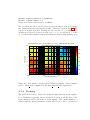
We will calculate the chosen model selection criterion over the grid defined by [arg8,arg9] = [0.001,1.0] kernel parameter and [arg11,arg12]
= [3,15] and cluster number ranges dividing up the kernel parameter range
into arg10=10 points using logarithmic spacing.
So we can execute the demo_kscicd_tune application:
[root@tecra demo]# ./demo_kscicd_tune 20000 2 158 40000 1 0.9 0
0.001 1.0 10 3 15 demo_data/io/ demo_data/G10_N1M/data_G10_K10_
ovl_Valid_40000
Comp. time of tuning: 85.59 [s]
Optimal kernel parameter:= 0.0215443
Optimal cluster number:= 10
Model selection criterion:= 0.935172
The computational time of the tuning was 85.59 seconds. The application
tested (CM AX − CM IN + 1) ∗ N H = 130 kernel parameter - cluster number
grid points with average computational time of 0.658 seconds at each grid
points. The optimal kernel parameter and cluster number values, that yield
the maximum model selection criterion 0.9351 , are 0.021 and 10. Note,
that a perfect KSC model would correspond to a maximal model selection
criterion value equal to 1. However, the 10 Gaussian distributions, that
the 1 million data points were sampled from, slightly overlap so perfect
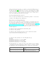
separation is not possible. We can check the whole model selection criterion surface (before accepting these values) by plotting the Q_m file. This
can be seen in Fig. 3.1. Note, that the application (or more exactly the
kscWkpcaIchol_tune function of the kscicd library) performs computations
only at discrete grid points. These results are smoothed in Fig. 3.1 that shows
that we can indeed accept these optimal values since the model selection criterion has a maximum around this point. We will use these parameters for
the training in the next step.
2
Performance over the [2σ ,C] grid; QMF=1; η=0.9; Ntr= 20000; R= 158; Nv= 40000
(interpolated between grid points)
14
1
0.9
0.8
12
C (#clusters)
0.7
10
0.6
0.5
8
0.4
6
0.3
0.2
4
0.1
0.001
0.01
0.1
1
kernel parameter (2σ2)
Figure 3.1: Performance over the selected kernel parameter - cluster number
grid i.e. the Q m file computed by the demo kscicd tune application.
3.3
Training the sparse KSC model
The demo_kscicd_train application trains the KSC model on the training
set by using the kscWkpcaIchol _tune function from the kscicd library.
Furthermore, it performs clustering of the training data points by using the
trained model and by calling the doClusteringAndCalcQuality function
from the kscicd library. The chosen model selection criterion value, corresponding to the training set clustering, is also calculated when calling the
doClusteringAndCalcQuality function. See sections 5.2 and 5.5 for the detailed description of the kscWkpcaIchol_train and doClusteringAndCalc
Quality functions.
The incomplete Cholesky factor matrix and the permuted training data
are inputs of the demo _kscicd_train application. It means that the demo_
ichol application must be executed before using demo_kscicd_train in order to ensure that both the res_icholfactor and the res_trainingdata
files are available in the io directory.
source code:
kscicd_package/util/src/demo/demo_kscicd_train.c
executable:
kscicd_package/demo/demo_kscicd_train <arg1> <arg2> ... <arg9>
Input parameters:
The corresponding kscWkpcaIchol_train and doClusteringAndCalcQuality
function parameters are indicated in the second and third columns of the table. See sections 5.2 and 5.5 for the detailed description of the kscWkpcaIchol
_train and doClusteringAndCalcQuality functions.
arguments
arg1
arg2
arg3
pars.
N
D
R
pars.
N
-
arg4
-
-
arg5
H
-
description
number of training data points;
dimension of training data points
number of columns in the incomplete
Cholesky factor obtained previously by using
the demo_ichol application (see section 3.1)
kernel function flag: =0→ RBF kernel, =1→
χ2 kernel
kernel parameter
arg6
arg7
C
QMF
C
QMF
arg8
-
ETA
arg9
-
-
number of desired clusters
model selection criterion flag (see further
notes on QMF parameter in section 5.2)
this is the η parameter value; the trade-off
between the collinearity measure and balance
terms of the selected model selection criterion
path to the io directory; some results of the
incomplete Cholesky decomposition, (like
the incomplete Cholesky factor matrix, permuted training data set) are stored in this io
directory and will need now
Output:
The application will train the sparse KSC model on the training set by
calling the kscWkpcaIchol_train function from the kscicd library. All
the data, determined during the training and necessary to construct the
sparse KSC model i.e. reduced set data, reduced set coefficients, codebook
and approximated bias terms (even in the case of QMF=1), will be written
into separate files located in the io directory as reduced_set_data_mtrx,
reduced_set_coef_mtrx, code_book_mtrx and reest_bias_terms_vect.
Furthermore, the application will use the trained model to cluster the training data points by calling doClusteringAndCalcQuality from the kscicd
library. The obtained result will be written into the res file located in the
current directory. Each row of the res file contains: (i.) the corresponding
training data point; ii.) plus additional information concerning the clustering stored in the corresponding row of the *RES matrix on termination of
the doClusteringAndCalcQuality. The information, available in the *RES
matrix regarding the clustering of the data points, depends on the chosen
model selection criterion because it also determines the cluster membership
encoding-decoding scheme. See further notes on the structure of the *RES
matrix at different QMF values in section 5.5 for more details.
Application:
The demo_kscicd_train application needs the incomplete Cholesky decomposition of the training set kernel matrix and the permuted training data
set. These can be obtained by executing the demo_ichol application (see
section 3.1). So the demo_ichol application must be executed before the
demo_kscicd_train in order to ensure that the res_icholfactor and res
_trainingdata files are available in the arg9=demo_data/io/ directory.
The res_trainingdata file stores the arg1 = 20000 permuted arg2 =
2 2D training data points and the res_icholfactor file contains the incomplete Cholesky factor matrix. The number of columns in the incomplete
Cholesky factor i.e. the exact value of arg3 will be determined at the termination of demo_ichol. We will use the arg4 = 0 RBF kernel, arg7 =
1 model selection criterion (see further notes on the QMF parameter in section 5.2) with an arg8= 0.9 trade-off parameter. This later means that the
collinearity measure part will be taken by a weight equal to 0.9 in the model
selection criterion while the weight of the balance measure part of the obtained clusters will be 1-arg8=0.1. The optimal number of clusters as well as
the optimal value of the RBF kernel parameter where determine beforehand
by using the demo_kscicd_tune application. Thus we set arg5 = 0.021 and
arg6 = 10.
So we can execute the demo_kscicd_train application:
[root@tecra demo]# ./demo_kscicd_train 20000 2 158 0 0.021 10 1
0.9 demo_data/io/
Comp. time of training: 0.88 [s]
Model selection criterion value:= 0.932464
The ordered cardinalities:
1.: 2581
2.: 2483
3.: 2285
4.: 2123
5.: 2064
6.: 1905
7.: 1788
8.: 1674
9.: 1632
10.: 1465
The demo_kscicd_train application (or more exactly the kscWkpcaIchol_train
function of the kscicd library) needs 0.88 seconds to train the sparse KSC
model on the training set and perform clustering on the training set points.
We will use this trained KSC model to cluster the full data set with 1 million
points in the next step.
3.4
Out-of-sample extension
The demo_kscicd_test application performs out-of-sample extension on the
test set by calling the kscWkpcaIchol _test and doClusteringAndCalcQual
ity functions from the kscicd library. The chosen model selection criterion
value, corresponding to the test set clustering, is also calculated when calling
the doClusteringAndCalcQuality function. See sections 5.3 and 5.5 for the
detailed description of the kscWkpcaIchol_test and doClusteringAndCalc
Quality functions.
The application requires all the data that are necessary to reconstruct
the sparse KSC model obtained at the training stage i.e. reduced set data,
reduced set coefficients, codebook and approximated bias terms (even in the
case of QMF=1). It means that the demo_kscicd_train application must be
executed before demo_kscicd_test in order to ensure that the reduced_set_
data_mtrx, reduced_set_coef_mtrx, code_book_mtrx and reest_bias_
terms_vect files are available in the io directory.
source code:
kscicd_package/util/src/demo/demo_kscicd_test.c
executable:
kscicd_package/demo/demo_kscicd_test <arg1> <arg2> ... <arg10>
Input parameters:
The corresponding kscWkpcaIchol_test and doClusteringAndCalcQuality
function parameters are indicated in the second and third columns of the table. See sections 5.3 and 5.5 for the detailed description of the kscWkpcaIchol
_test and doClusteringAndCalcQuality functions.
arguments
arg1
arg2
pars.
N
D
pars.
N
-
arg3
R
-
arg4
-
-
description
number of test data points;
dimension of the data points; same as in the
training
number of reduced set points; same as the
rank of the ICD obtained previously by using
the demo_ichol application (see section 3.1)
kernel function flag: =0→ RBF kernel, =1→
χ2 kernel; same as in the training
arg5
arg6
arg7
H
C
QMF
C
QMF
arg8
-
ETA
arg9
-
-
arg10
-
-
kernel parameter; same as in the training
number of clusters; same as in the training
model selection criterion flag (see further
notes on QMF parameter in section 5.2); same
as in the training
this is the η parameter value; the trade-off
between the collinearity measure and balance
terms of the selected model selection criterion
path to the io directory; some results of the
training (files listed above) are stored in this
io directory and will need now
path to the test data file
Output:
The application will reconstruct the sparse KSC model obtained at the training stage and will perform clustering of test points i. e.clustering of arbitrary
input data points by calling the kscWkpcaIchol_test and doClusteringAnd
CalcQuality functions from the kscicd library.
The obtained result will be written into the res file located in the current directory. Each row of the res file contains: (i.) the corresponding
training data point; ii.) plus additional information concerning the clustering stored in the corresponding row of the *RES matrix on termination of
the doClusteringAndCalcQuality. The information, available in the *RES
matrix regarding the clustering of the data points, depends on the chosen
model selection criterion because it also determines the cluster membership
encoding-decoding scheme. See further notes on the structure of the *RES
matrix at different QMF values in section 5.5 for more details.
Application:
The demo_kscicd_test application needs some data to reconstruct the sparse
KSC model obtained at the training stage i.e. reduced set data, reduced
set coefficients, codebook and approximated bias terms (even in the case of
QMF=1). It means that the demo_kscicd_train application must be executed
before demo_kscicd_test in order to ensure that the reduced_set_data_mtrx,
reduced_set_coef_mtrx, code_book_mtrx and reest_bias_terms_vect files
are available in the arg9=demo_data/io/ directory.
We want to extend the clustering to the full data set now. The arg1 = 106
arg2 = 2 2D full data set points are stored in the arg10 = demo_data/G10_N1M/
data_G10_K10_ovl_Full_1E6 file. The number of reduced set points i.e. the
exact value of arg3 will be determined at the termination of demo_ichol as
the rank of the approximation. As in the training, we will use the arg4 = 0
RBF kernel, arg7 = 1 model selection criterion (see further notes on the QMF
parameter in section 5.2) with an arg8= 0.9 trade-off parameter. This later
means that the collinearity measure part will be taken by a weight equal to
0.9 in the model selection criterion while the weight of the balance measure
part of the obtained clusters will be 1-arg8=0.1. The number of clusters
as well as the RBF kernel parameter value must also be the same as in the
training arg5 = 0.021 and arg6 = 10.
So we can execute the demo_kscicd_test application:
[root@tecra demo]# ./demo_kscicd_test 1000000 2 158 0 0.021 10 1
0.9 demo_data/io/ demo_data/G10_N1M/data_G10_K10_ovl_Full_1E6
Comp. time of clustering: 13.29 [s]
Model selection criterion value:= 0.974777
The ordered cardinalities:
1.: 100282
2.: 100155
3.: 100040
4.: 100018
5.: 99998
6.: 99990
7.: 99955
8.: 99917
9.: 99848
10.: 99797
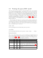
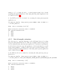
Clustering the full data set with 1 million points takes 13.29 seconds by
using the trained model and its out-of-sample capability. The results are
written into the current directory as a res file. We used the model selection
criterion QMF=1 so each line of the res file contains one of the 2 D input
data points (order is the same as in the data_G10_K10_ovl_Full_1E6 file)
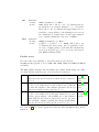
plus the obtained cluster membership label and a clustering quality measure.
These are plotted in Fig.3.2 and Fig.3.3 respectively.
Clustering results on the G10_N1M data set
(plotted only every 10th points out of 1 million)
2
10
1.5
9
1
8
0.5
7
0
6
-0.5
5
-1
4
-1.5
3
-2
2
-2.5
-2.5
1
-2
-1.5
-1
-0.5
0
0.5
1
1.5
2
2.5
Figure 3.2: Clustering results on the G10 N1M data set by using the trained
KSC model.
Clustering quality on the G10_N1M data set
(plotted only every 10th points out of 1 million)
2
1
1.5
0.9
1
0.8
0.7
0.5
0.6
0
0.5
-0.5
0.4
-1
0.3
-1.5
0.2
-2
-2.5
-2.5
0.1
0
-2
-1.5
-1
-0.5
0
0.5
1
1.5
2
2.5
Figure 3.3: Clustering quality for each point plotted in Fig.3.2. Note that
points that are close to the decision boundary of the KSC model have a lower
quality value.
Chapter 4
Example
The demo applications are discussed in chapter 3 by using the G10_N1M demo
data set. Further examples will be presented in this chapter by using the
demo applications. All the details concerning the input parameters and the
descriptions of the demo applications can be found in chapter 3. Therefore,
the different applications will be executed here without detailed explanation
of the meaning of the chosen parameter values.
4.1
4.1.1
Image segmentation
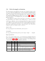
The IMG BID 145086 Q8 data set
The IMG_BID_145086_Q8 data set will be used in this example that you
can download from kscicd page http://esca.atomki.hu/~novmis/kscicd.
This data set was generated by using one of the color images (imageID
145086) from the Berkeley image data set 1 . The RGB color image has
N = 321 x 481 = 154 401 pixels. A local color histograms was computed at
each pixel by taking a 5 x 5 window around the pixel using minimum variance color quantization of eight levels. After normalization, the N = 154 401
histograms serve the 8 dimensional input data points of IMG_BID_145086_Q8
data set.
Go to your kscicd_package/demo/demo _data/ subdirectory, download
IMG_BID_145086_Q8.tar.gz into this directory and uncompress it:
[root@tecra kscicd_package]# cd demo/demo_data
[root@tecra demo_data]#
1
http://www.eecs.berkeley.edu/Research/Projects/CS/vision/grouping/segbench/
27
[root@tecra demo_data]# wget http://esca.atomki.hu/~novmis/
kscicd/html/downloads/IMG_BID_145086_Q8.tar.gz
...
...
...
[root@tecra demo_data]# tar -zxvf IMG_BID_145086_Q8.tar.gz
IMG_BID_145086_Q8/
IMG_BID_145086_Q8/data_BID145086_Q8_N154401
IMG_BID_145086_Q8/data_BID145086_Q8_Full_N154401
IMG_BID_145086_Q8/data_BID145086_Q8_Train_N10000
IMG_BID_145086_Q8/data_BID145086_Q8_Valid_N30000
The IMG_BID_145086_Q8 directory contains the following files:
data_BID145086_Q8_N154401
data_BID145086_Q8_Full_N154401
data_BID145086_Q8_Train_N10000
data_BID145086_Q8_Valid_N30000
vertical pixels, horizontal pixels
and the normalized local color
histogram for each of the N = 154
401 pixels
the normalized local color
histograms
taken
from
data_BID145086_Q8_N154401;
these N = 154 401, 8-dimensional
points form the full data set
10 000 data points for training;
sampled randomly from the full
data set
30 000 data points for validation;
the union of the 10 000 training data points and 20 000 additional data points sampled randomly from the remaining part of
the full data set
The χ2 kernel will be used in this chapter that is implemented in the kscicd_
package/util/src/demo/kscicd_kerns.c source file that is included into
each demo application. (see the notes on the kernel function implementation
at the beginning of chapter 5 for more details).
4.1.2
Incomplete Cholesky decomposition
The demo_ichol application can be used to perform the ICD step on the
training data kernel matrix: The χ2 kernel (arg3=1) will be used with a kernel parameter value of 0.05 (arg4=0.05). The tolerance value of the ICD and
the maximum rank of the approximation will be set to 0.5 (arg5=0.5) and
200 (arg6=200) respectively. More details regarding the input parameters of
the demo_ichol application can be found in section 3.1
So the incomplete Cholesky decomposition of the training set kernel matrix
can be performed by the means of demo_ichol application as:
[root@tecra demo]# ./demo_ichol 10000 8 1 0.05 0.5 200 demo_
data/io/ demo_data/IMG_BID_145086_Q8/data_BID145086_Q8_Train_
N10000
Time: = 1.25 [s]
Rank: = 200
Tol: = 0.507157
4.1.3
Tuning
The optimal number of clusters and kernel parameter values can be determined through a grid search. This KSC model tuning can be done by using the demo_kscicd_tune application. The model selection criterion corresponds to QMF=1 (arg5=1) will be used giving all the weights to the collinearity measure part of the model selection criterion i.e. η = 1.0 (arg6=1.0). The
maximum value will be searched over a grid defined by the [H_MIN,H_MAX] =
[0.001,1.0] (arg8=0.01, arg9=1.0,) kernel parameter and [C_MIN,C_MAX]
= [3,10] (arg11=3, arg12=10,) cluster number intervals. The kernel parameter interval will be divided up to 10 points (arg10=10) using logarithmic
spacing. More details regarding the input parameters of the demo_kscicd_tune
application can be found in section 3.2
So the KSC model parameter tuning can be done by executing the demo_kscicd_tune
application as:
[root@tecra demo]# ./demo_kscicd_tune 10000 8 200 30000 1 1.0
1 0.001 1.0 10 3 10 demo_data/io/ demo_data/IMG_BID_145086_Q8/
data_BID145086_Q8_Valid_N30000
Comp. time of tuning: 78.47 [s]
Optimal kernel parameter:= 0.0464159
Optimal cluster number:= 3
Model selection criterion:= 0.936852
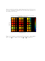
We can check the whole model selection criterion surface (before accepting
the optimal values) by plotting the Q_m file. This can be seen in Fig. 4.1. We
can see from this plot, that dividing the data set into C = 4 clusters gives
as high model selection criterion value as C = 3. So we will use C = 4 and
σχ = 0.0464 cluster number and kernel parameter values in the training step.
C (#clusters)
Performance over the [σχ,C] grid; QMF=1; η=1.0; Ntr= 10000; R= 200; Nv= 30000
(interpolated between grid points)
10
9
0.9
8
0.8
7
0.7
6
0.6
5
0.5
4
0.4
3
0.001
0.3
0.01
0.1
1
kernel parameter (σχ)
Figure 4.1: Performance over the selected kernel parameter - cluster number
grid i.e. the Q m file computed by the demo kscicd tune application.
4.1.4
1
Training
The KSC model can be trained by using the demo_kscicd_train application. Parameters regarding the model selection criterion and the type of the
kernel function will be the same as in the tuning. The optimal number of
clusters and the kernel parameter values will be set to those obtained by
tuning i.e. C = 4 (arg6=4) and σχ = 0.0464 (arg5=0.0464). More details
regarding the input parameters of the demo_kscicd_train application can
be found in section 3.3
So the KSC model can be trained by executing the demo_kscicd_train
application as:
[root@tecra demo]# ./demo_kscicd_train 10000 8 200 1 0.0464 4 1
1.0 demo_data/io/
Comp. time of training: 0.65 [s]
Model selection criterion value:= 0.936335
The ordered cardinalities:
1.: 4601
2.: 2350
3.: 1541
4.: 1508
4.1.5
Out-of-sample extension
The last step is to perform clustering on the full input data set by using
the previously trained KSC model. This out-of-sample extension step can be
done by using the demo_kscicd_test application. Parameters regarding the
model selection criterion, type and parameter of the kernel function as well
as the desired number of clusters will be the same as in the training. More
details regarding the input parameters of the demo_kscicd_test application
can be found in section 3.4
So the KSC model can be trained by executing the demo_kscicd_test application as:
[root@tecra demo]# ./demo_kscicd_test 154401 8 200 1 0.0464 4 1
1.0 demo_data/io/ demo_data/IMG_BID_145086_Q8/data_BID145086_Q8_Full_N154401
Comp. time of clustering: 4 [s]
Model selection criterion value:= 0.936258
The ordered cardinalities:
1.: 65131
2.: 41850
3.: 25212
4.: 22208
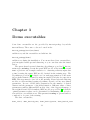
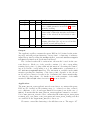
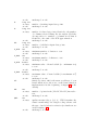
You can merge the first two columns from the data_BID145086_Q8_N154401
file (i.e. vertical pixels and horizontal pixels) and the 9th column from the
res file (i.e. the obtained cluster label). If you do so and plot the resulted
image you will see something like Fig. 4.2
Image (ID 145086) segmentation result
σχ=0.0464; C=4; Ntr=10000; R=200; N=154401
Table 4.2: Top: the original image (image ID= 145086); Bottom: segmented image obtained by using the kscicd package.
Chapter 5
List of functions
A detailed list of functions available in the kscicd library is provided here
with their descriptions:
5.1 ichol :: for the incomplete Cholesky decomposition
5.2 kscWkpcaIchol_train :: for training the KSC model
5.3 kscWkpcaIchol_test :: for doing out-of-sample extension
5.4 kscWkpcaIchol_tune :: for model selection
5.5 doClusteringAndCalcQuality :: for cluster assignment
Some notes on data format and matrix representation
The kscicd C library is based on LAPACK and BLAS libraries that are
written in FORTRAN. The LAPACK and BLAS libraries store matrices in
the memory as 1D arrays in column-major format. The same data format
was adopted in the kscicd C library in order to avoid unnecessary data
transformations before/after calling routines from the LAPACK and BLAS
libraries.
In the case of demo executables you will need to feed the applications with
files containing different input data (for training, for validation, ect.). It is
assumed that your data pints are stored in your input files line by line. So
the files contain as many lines as data points are stored in the file and the
number of columns is equal to the dimension of the data points.
35
Some notes on the kernel function implementation
The kscicd library does not contain any kernel function implementations.
In order to give the highest level of flexibility, a function pointer
double(*kern_func)(double*,long int,long int,double*,
long int,long int,long int,double)
is used in the library. This pointer must set to the address of your own kernel
function by passing its memory address as function parameter. Your kernel
function is assumed to be implemented in the following form:
double yourKernelFunctionName(double *M1,long int i,long int Ni,
double *M2,long int j,long int Nj,long int dim, double
kernPar){
/*
your kernel function implementation
including a (double) return value
*/
}
where
the memory address of the RNi×dim matrix in which
the first argument of the kernel function is stored (the
matrix is stored in the memory as 1D array in columnmajor format)
long int i:
the row index of the first argument of the kernel function in *M1
long int Ni:
number of rows in *M1
double *M2:
the memory address of the RNj×dim matrix in which
the second argument of the kernel function is stored
(the matrix is stored in the memory as 1D array in
column-major format)
long int j:
the row index of the second argument of the kernel
function in *M2
long int Nj:
number of rows in *M2
long int dim:
dimension of the input data points i.e. number of
columns in *M1 and *M2
double kernPar: the kernel parameter
double *M1:
These parameters will be set to the appropriate values in each kernel function
call by the corresponding functions of the kscicd library. You can see a radial
basis function (RBF) kernel implementation below as an example in the form
of K(¯
xi , x¯j ) = exp(−k¯
xi − x¯j k22 /(2σ 2 )); x¯ ∈ Rd and kernPar = 2σ 2 , dim = d:
/* RBF kernel implementation example */
double kernFunc(double *M1, long int i, long int Ni, double *M2,
long int j, long int Nj,
long int dim, double kernPar){
long int k;
double dummy0,dummy1;
dummy0=0.0;
for(k=0;k<dim;++k)
{
dummy1=m1[i+k*Ni]-m2[j+k*Nj];
dummy0+=dummy1*dummy1;
}
return exp(-1.0*dummy0/kernPar);
}
// you can pass the address as &kernFunc //
The RBF and χ2 kernels, used in the demo applications, are implemented in
the kscicd_package/util/src/demo/kscicd_kerns.c that is included into
each demo application. You can implement your own kernel similarly in your
applications.
5.1
ichol
Purpose
Calculate the incomplete Cholesky decomposition of the training set kernel
matrix. Terminates when either the TOL tolerance limit or the R maximum
rank of the approximation is reached.
Syntax
void ichol(double *A, long int N, long int D, double H, double
(*KF) (double*, long int, long int, double*, long int, long
int, long int, double), double **G, long int **P, double *TOL,
long int *R);
Parameters
A:
N:
D:
H:
double*
on entry:
on exit:
long int
on entry:
on exit:
long int
on entry:
on exit:
double
on entry:
on exit:
KF:
G:
double**
on entry:
on exit:
*A is the memory address of an 1D array where
your N , D-dimensional training input data are
stored in a column-major format
unchanged on exit
number of training input data points
unchanged on exit
dimension of input data points
unchanged on exit
kernel width (i.e. 2σ 2 )
unchanged on exit
function pointer; *KF is the memory address of
your kernel function (see the notes on the kernel
function implementation at the beginning of chapter 5 for the details)
*G is assumed to be NULL
*G will point to the N × R-dimensional incomplete
Cholesky factor i.e. to a 1D array where the N ×
R elements of the incomplete Cholesky factor are
stored in column-major format
P:
long int**
on entry:
on exit:
TOL: double*
on entry:
on exit:
R:
long int*
on entry:
on exit:
*P is assumed to be NULL
*P will point to an 1D array with N elements
where permuted indices of the N training input
data points are stored
*TOL is the memory address where the tolerance
value of the incomplete Cholesky decomposition is
stored
the pointed memory is overwritten by the exact
error value corresponding to the obtained incomplete Cholesky decomposition of the training set
kernel matrix
*R is the memory address where the maximally
allowed rank (i.e. maximum number of selected
columns in the incomplete Cholesky decomposition) is stored
the pointed memory is overwritten by the exact
rank corresponding to the obtained incomplete
Cholesky decomposition of the training set kernel
matrix
Further notes
You can set R=N if you want to control the ICD entirely by the TOL value.
It is the caller responsibility to free the memory allocated in ichol to store
the G matrix and the P vector.
See section 3.1 for a demo application that use this ichol function.
5.2
kscWkpcaIchol train
Purpose
Train a sparse kernel spectral clustering model on the training set based on
the incomplete Cholesky decomposition of the training set kernel matrix.
Syntax
void kscWkpcaIchol_train(double *TRD, long int D, double *G, long
int N, long int R, int C, double H, double (*KF) (double*, long
int, long int, double*, long int, long int, long int, double),
int QMF, double **RSC, double **CB, double **REB, double **ASV,
double **SCOV);
Parameters
TRD:
D:
G:
N:
double*
on entry:
*TRD is the memory address of an 1D array where
your N , D-dimensional permuted training data are
stored in a column-major format (NOTE, that it is assumed that the training data are reordered according
to the permutations done in the incomplete Cholesky
decomposition)
unchanged on exit
on exit:
long int
on entry: dimension of input data points
on exit:
unchanged on exit
double*
on entry: *G is the memory address where the N × Rdimensional incomplete Cholesky factor i.e. the memory address of an 1D array where the N × R elements of the incomplete Cholesky factor are stored in
column-major format (the incomplete Cholesky factor can be obtained by calling the ichol functions on
the training set)
on exit:
the pointed memory will be freed since the memory
content will be destroyed during the training
long int
on entry: number of training input data points
R:
C:
H:
KF:
QMF:
RSC:
CB:
REB:
on exit:
unchanged on exit
long int
on entry: number of columns selected during the incomplete
Cholesky decomposition i.e. number of columns in
∗G that is identical to the rank of the ICD approximation or identical to the number of reduced set points
on exit:
unchanged on exit
int
on entry: number of desired clusters
on exit:
unchanged on exit
double
on entry: kernel width (i.e. 2σ 2 )
on exit:
unchanged on exit
function pointer; *KF is the memory address of your
kernel function (see the notes on the kernel function
implementation at the beginning of chapter 5 for the
details)
int
on entry: quality measure flag ∈ [0, 1, 2]. Will determine the
cluster membership encoding-decoding scheme and
the type of model selection criterion. See further
notes below!
on exit:
unchanged on exit
double**
on entry: *RSC is assumed to be NULL
on exit:
*RSC will point to the R×(C −1) dimensional reduced
set coefficient matrix i.e. to a 1D array where the R,
(C −1)-dimensional reduced set coefficients are stored
in column-major format
double**
on entry: *CB is assumed to be NULL
on exit:
*CB will point to the C × (C − 1) dimensional codebook matrix i.e. to a 1D array where the C, (C −
1)-dimensional prototype code words are stored in
column-major format (NOTE, that the type of the
codewords depends on the chosen QM F value)
double**
on entry: *REB is assumed to be NULL
on exit:
*REB will point to the (C − 1) dimensional approximated bias term vector i.e. to a 1D array where the
(C − 1) approximated bias terms are stored
ASV:
double**
on entry: *ASV is assumed to be NULL
on exit:
*ASV will point to the N × (C − 1) dimensional approximated score variable matrix i.e. to a 1D array
where the N , (C −1)-dimensional approximated score
variables corresponding to the training set are stored
in column-major format; these are the approximated
score variables minus the bias vector if QMF=1
SCOV: double**
on entry: *SCOV is assumed to be NULL
on exit:
if QM F = 0 and C = 2, *SCOV will point to an
N dimensional array where the N elements of the
second coordinate values for the Line Fit calculations
are stored; if QM F 6= 0 or C > 2 it is not referenced
and *SCOV remains NULL
Further notes
It is the caller responsibility to free the memory allocated in
kscWkpcaIchol_train to store *RSC, *CB, *REB, *ASV and *SCOV (if QMF=0
and C=2).
The QMF quality measure flag determines the cluster membership encodingdecoding scheme and the type of model selection criterion:
QMF=0
QMF=1
QMF=2
sign based encoding-decoding scheme and BLF model
selection; the model selection criterion can be used for
C≥2
angular similarity based encoding-decoding scheme;
codebook is built based on the reduced set coefficient
points and angular cosine distance measure; the model
selection criterion can be used for C > 2
angular similarity based encoding-decoding scheme;
codebook is built based on the approximated score variables corresponding to the training set; cosine distance
and AMS model selection criterion is used to produce
probabilistic outputs regarding the cluster membership;
the model selection criterion can be used for C > 2
see [3] for
further details
see [1] for
further details
see
[13]
for further
details
See section 3.3 for a demo application that use this kscWkpcaIchol_train
function.
5.3
kscWkpcaIchol test
Extends the kernel spectral clustering model, obtained on the training set by
means of kscWkpcaIchol_train to unseen data points.
Syntax
void kscWkpcaIchol_test(double *TED,long int N,long int D, double
*RSD, long int R, int C, double H, double (*KF) (double*, long
int, long int, double*, long int, long int, long int, double),
int QMF, double *RSC, double *CB, double *REB, double **ASV,
double **SCOV);
Parameters
TED:
N:
D:
RSD:
R:
double*
on entry:
on exit:
long int
on entry:
on exit:
long int
on entry:
on exit:
double *
on entry:
points to the 1D array where your N , D-dimensional
test data are stored in a column-major format
unchanged on exit
number of test input data points
unchanged on exit
dimension of input data points
unchanged on exit
points to the 1D array where the R, D-dimensional
reduced set data are stored in column-major format;
these are the R input data points selected from the
training set as pivots during the incomplete Cholesky
decomposition; NOTE that it is assumed that these
R data points are reordered according to the permutations done during the ICD
unchanged on exit
on exit:
long int
on entry: number of reduced set points; identical to the number
of columns selected during the incomplete Cholesky
decomposition i.e. number of columns in ∗G that is
identical to the rank of the ICD approximation
on exit:
unchanged on exit
C:
H:
int
on entry:
on exit:
double
on entry:
on exit:
KF:
QMF:
RSC:
CB:
REB:
ASV:
int
on entry:
on exit:
double*
on entry:
on exit:
double*
on entry:
on exit:
double*
on entry:
number of desired clusters; same as in the training
unchanged on exit
kernel width (i.e. 2σ 2 ); same as in the training
unchanged on exit
function pointer; *KF is the memory address of your
kernel function (see the notes on the kernel function
implementation at the beginning of chapter 5 for the
details)
quality measure flag ∈ [0, 1, 2]. Will determine the
cluster membership encoding-decoding scheme and
the type of model selection criterion. Same as in the
training (see further notes at the training 5.2)
unchanged on exit
points to the R × (C − 1) dimensional reduced set
coefficient matrix obtained during the training i.e. to
a 1D array where the R, (C − 1)-dimensional reduced
set coefficients are stored in column-major format; it
is *RSC on exit from kscWkpcaIchol_train
unchanged on exit
points to the C×(C−1) dimensional codebook matrix
i.e. to a 1D array where the C, (C − 1)-dimensional
prototype codewords are stored in column-major format (NOTE, that the type of the codewords depends
on the QM F value chosen at the training stage); it
is *CB on exit from kscWkpcaIchol_train
unchanged on exit
points to the (C − 1) dimensional approximated bias
term vector i.e. to a 1D array where the (C − 1)
approximated bias terms are stored; it is *REB on
exit from kscWkpcaIchol_train
unchanged on exit
on exit:
double**
on entry: *ASV is assumed to be NULL
on exit:
*ASV will point to the N × (C − 1) dimensional approximated score variable matrix i.e. to a 1D array where the N , (C − 1)-dimensional approximated
score variables corresponding to the test set are stored
in column-major format; these are the approximated
score variables minus the bias vector if QMF=1
SCOV: double**
on entry: *SCOV is assumed to be NULL
on exit:
if QM F = 0 and C = 2, *SCOV will point to an
N dimensional array where the N elements of the
second coordinate values for the Line Fit calculations
are stored; if QM F 6= 0 or C > 2 it is not referenced
and *SCOV remains NULL
Further notes
It is the caller responsibility to free the memory allocated in
kscWkpcaIchol_test to store *ASV and *SCOV (if QMF=0 and C=2).
See section 3.4 for a demo application that use this kscWkpcaIchol_test
function.
5.4
kscWkpcaIchol tune
Calculates the model selection criterion surface over a cluster number - kernel
parameter grid. The optimal cluster number and kernel parameter (i.e. the
optimal kernel spectral clustering model) can be selected by the analysis
of this surface. A sparse kernel spectral clustering model is trained on the
training set at each point of the cluster number-kernel parameter grid and the
trained model is used to perform out-of-sample extension on the validation
set. Then the model selection criterion is evaluated on the clustering results
obtained on the validation set.
Syntax
void kscWkpcaIchol_tune(double *TRD, double *VD, long int D,
double *G, long int N, long int R, long int NV, int C_MIN, int
C_MAX, double H_MIN, double H_MAX, double (*KF) (double*, long
int, long int, double*, long int, long int, long int, double),
int NH, int QMF, double ETA, double **OPTHP, double **QM);
Parameters
TRD:
VD:
D:
G:
double*
on entry:
on exit:
double*
on entry:
points to the 1D array where your N , D-dimensional
training data are stored in a column-major format
unchanged on exit
points to the 1D array where your N V , Ddimensional validation data are stored in a columnmajor format
unchanged on exit
on exit:
long int
on entry: dimension of input data points
on exit:
unchanged on exit
double*
on entry: points to to the N × R-dimensional incomplete
Cholesky factor i.e. to a 1D array where the N × R
elements of the incomplete Cholesky factor (obtained
on the training set) are stored in column-major format (G can be obtained by calling the ichol functions on the training set)
N:
R:
on exit:
long int
on entry:
on exit:
long int
on entry:
on exit:
long int
on entry:
on exit:
C_MIN: int
on entry:
on exit:
C_MAX: int
on entry:
on exit:
H_MIN: double
on entry:
unchanged on exit
number of training input data points
unchanged on exit
number of reduced set points; identical to the number
of columns selected during the incomplete Cholesky
decomposition i.e. number of columns in ∗G that is
identical to the rank of the ICD approximation
unchanged on exit
NV:
on exit:
H_MAX: double
on entry:
on exit:
KF:
NH:
QMF:
int
on entry:
on exit:
int
on entry:
on exit:
number of validation input data points
unchanged on exit
minimum number of clusters to test
unchanged on exit
maximum number of clusters to test
unchanged on exit
minimum value of kernel width (i.e. minimum 2σ 2 )
to test
unchanged on exit
maximum value of kernel width (i.e.maximum 2σ 2 )
to test
unchanged on exit
function pointer; *KF is the memory address of your
kernel function (see the notes on the kernel function
implementation at the beginning of chapter 5 for the
details)
number of points in the [HM IN, HM AX] interval to
test
unchanged on exit
quality measure flag ∈ [0, 1, 2]. Will determine the
cluster membership encoding-decoding scheme and
the type of model selection criterion (see further notes
at the training 5.2)
unchanged on exit
ETA:
double
on entry:
∈ [0, 1] is the trade off between the collinearity measure corresponding to the chosen QM F and the balance of the obtained clusters. The calculated model
selection criterion is based entirely of the collinearity
measure if ET A = 1 and solely on the balance of the
obtained clusters if ET A = 0. (see [3, 1] for further
details)
unchanged on exit
on exit:
OPTHP: double**
on entry: *OPTHP is assumed to be NULL
on exit:
*OPTHP will point to vector with the following elements:
*OPTHP[0]=optimal kernel paramter,
*OPTHP[1]=optimal number of clusters,
*OPTHP[2]=optimal model selection criterion
value, where optimality corresponds to the maximum of the model selection criterion; however, it is
ALWAYS recommended to examine the whole grid
before accepting these optimal parameter values
QM:
double**
on entry: *QM is assumed to be NULL
on exit:
*QM will point to matrix with the elements of the
tested kernel parameter values and cluster number
grid points and the corresponding model selection criterion value. See further notes below for more details.
Further notes
It is the caller responsibility to free the memory allocated in
kscWkpcaIchol_tune to store *OPTHP and *QM.
The 2D cluster number-kernel parameter grid is generated in the following
way: each point in the [C_MIN, C_MAX] cluster number interval is taken; NH
points are taken by logarithmically spacing the [H_MIN, H_MAX] kernel parameter interval; thus the grid contains (C_MAX-CMIN+1)×NH cluster numberkernel parameter point pairs; at each point pairs: first the sparse KSC model
is trained on the training set, then the trained model is used to cluster the
points in the validation set, then the model selection criterion is evaluated
on the clustering results obtained on the validation set.
The QM matrix is stored in column-major format and it has the following
structure:
X
H_MIN
..
.
C_MIN
value
..
.
...
...
...
C_MAX
value
..
.
H_MAX
value
...
value
See section 3.2 for a demo application that use this kscWkpcaIchol_tune
function.
5.5
doClusteringAndCalcQuality
Perform the cluster membership decoding i.e. explicit clustering of the data
points (training or test points) based on the approximated score variables
(obtained on the training or on the test set) and the codebook. Furthermore, calculate the model selection criterion depending on the selected cluster membership encoding-decoding scheme (i.e. on the selected QMF value).
Syntax
void doClusteringAndCalcQuality(int QMF, double ETA, long int N,
long int C, double *CB, double *ASV, double *SCOV, double
**RES, double **MSV);
Parameters
QMF:
ETA:
N:
C:
int
on entry:
on exit:
double
on entry:
quality measure flag ∈ [0, 1, 2]. Will determine the
cluster membership encoding-decoding scheme and
the type of model selection criterion. Same as in the
training stage. (see further notes at the training 5.2)
unchanged on exit
∈ [0, 1] is the trade off between the collinearity measure corresponding to the chosen QM F and the balance of the obtained clusters. The calculated model
selection criterion is based solely on the collinearity
measure if ET A = 1 and solely on the balance of the
obtained clusters if ET A = 0. (see [3, 1] for further
details)
unchanged on exit
on exit:
long int
on entry: number of score points (same as the number of training data points or same as the the number of test
data points
on exit:
unchanged on exit
int
on entry: number of clusters; (same as in the training and the
test)
on exit:
unchanged on exit
CB:
ASV:
double*
on entry:
on exit:
double*
on entry:
on exit:
SCOV: double*
on entry:
RES:
MSV:
points to the C×(C−1) dimensional codebook matrix
i.e. to a 1D array where the C, (C − 1)-dimensional
prototype codewords are stored in column-major format (NOTE, that the type of the codewords depends
on the QM F value chosen at the training stage); it
is *CB on exit from kscWkpcaIchol_train
unchanged on exit
point to the N × (C − 1) dimensional approximated score variable matrix i.e. to a 1D array
where the N , (C − 1)-dimensional approximated
score variables corresponding to the training/or to
the test set are stored in column-major format; it
is *ASV on exit from kscWkpcaIchol_train/or from
kscWkpcaIchol_test; these are the approximated
score variables minus the bias vector if QMF=1
unchanged on exit
points to an N dimensional array where the N elements of the second coordinate values for the Line
Fit calculations are stored if QM F = 0 and C = 2;
if QM F 6= 0 or C > 2 it is not referenced
the pointed memory is freed on exit
on exit:
double**
on entry: *RES is assumed to be NULL
on exit:
*RES will point to a matrix where the results of the
clustering are stored. See further details below.
double**
on entry: *MSV is assumed to be NULL
on exit:
*MSV will point to a C + 1 dimensional vector. The
first element stores the model selection value calculated on the clustering result. The next C elements
are the cardinalities of the clusters in descending order.
Further notes
The structure of the matrix pointed by *RES depends on the selected QMF
value:
if QMF=0:
if QMF=1:
if QMF=2:
it points to an N dimensional vector i.e. to an 1D
array where the cluster indicators of the N points
are stored;
it points to an N ×2 dimensional matrix i.e. to an 1D
array where the N cluster indicators and the corresponding clustering quality measure values are stored
in column-major order (see [1] for further details);
it points to an N × (C + 2) dimensional matrix i.e.
to an 1D array where following data are stored in
column-major format: the N cluster indicators are
stored in the first column; the corresponding cluster
membership probability is stored in the second column; the different cluster membership probabilities
are stored in the following C columns; (see [13] for
further details);
It is the caller responsibility to free the memory allocated in
doClusteringAndCalcQuality to store *RES and *MSV.
See section 3.3 or 3.4 for demo applications that use this doClusteringAndCalcQuality
function.
Bibliography
[1] M. Nov´ak, C. Alzate, R. Langone, J.A.K. Suykens, Fast kernel spectral
clustering based on incomplete Cholesky factorization for large scale
data analysis, to be published
[2] C. Alzate, J.A.K. Suykens, Sparse kernel models for spectral clustering
using the incomplete Cholesky decomposition, in: Proceedings of the
2008 International Joint Conference on Neural Networks (IJCNN 2008),
(2008), 3555–3562
[3] C. Alzate, J.A.K. Suykens, Multiway spectral clustering with out-ofsample extensions through weighted kernel PCA, IEEE Transactions
On Pattern Analysis And Machine Intelligence 32(2), (2010), 335-347
[4] J.A.K. Suykens, T. Van Gestel, J. De Brabanter, B. De Moor, J. Vandewalle, Least Squares Support Vector Machines, World Scientific, Singapore, (2002)
[5] B. Sch¨olkopf, S. Mika, C.J.C. Burges, P. Knirsch, K. R. M¨
uller, G.
R¨atsch, A. Smola, Input space vs. feature space in kernel-based methods,
IEEE Transactions on Neural Networks, 10(5), (1999), 1000–1017
[6] S Fine, K Scheinberg, Efficient SVM training using low-rank kernel representations, The Journal of Machine Learning Research 2, (2002), 243264
[7] F.R. Bach, M.I. Jordan, Kernel independent component analysis, The
Journal of Machine Learning Research 3, (2002), 1-48
[8] E. Anderson, Z. Bai,C. Bischof, S. Blackford, J. Demmel, J. Dongarra,
J. Du Croz, A. Greenbaum, S. Hammarling, A. McKenney, S. Sorensen,
LAPACK Users’ Guide (Third ed.), ( 1999), Philadelphia, PA: Society
for Industrial and Applied Mathematics, ISBN 0-89871-447-8
53
[9] C. L. Lawson, R. J. Hanson, D. Kincaid, and F. T. Krogh, Basic Linear Algebra Subprograms for FORTRAN usage, ACM Transactions on
Mathematical Software, 5 (1979), 308-323
[10] L. S. Blackford, J. Demmel, J. Dongarra, I. Duff, S. Hammarling, G.
Henry, M. Heroux, L. Kaufman, A. Lumsdaine, A. Petitet, R. Pozo,
K. Remington, R. C. Whaley, An Updated Set of Basic Linear Algebra
Subprograms (BLAS), ACM Transactions on Mathematical Software
28(2), (2002), 135-151
[11] R.C. Whaley, A. Petitet,J.J. Dongarra, Automated Empirical Optimization of Software and the ATLAS Project, Parallel Computing 27, (2001),
3–35
[12] http://math-atlas.sourceforge.net/
[13] R. Langone,R. Mall, J.A.K. Suykens, Soft Kernel Spectral Clustering,
in Proc. of the (IJCNN 2013), Dallas, Texas, (2013) , 1028-1035