Download Computer-Assisted Troubleshooting for Efficient Off-board

Linköping Studies in Science and Technology
Thesis No. 1490
Computer-Assisted Troubleshooting
for Efficient Off-board Diagnosis
Håkan Warnquist
Department of Computer and Information Science
Linköpings universitet, SE–581 83 Linköping, Sweden
Linköping 2011
c Håkan Warnquist, 2011
Copyright ISBN 978-91-7393-151-9
ISSN 0280-7971
Printed by LiU Tryck 2011
URL: http://urn.kb.se/resolve?urn=urn:nbn:se:liu:diva-67522
i
Computer-Assisted Troubleshooting
for Efficient Off-board Diagnosis
by
Håkan Warnquist
June 2011
ISBN 978-91-7393-151-9
Linköping Studies in Science and Technology
Thesis No. 1490
ISSN 0280-7971
LiU–Tek–Lic–2011:29
ABSTRACT
This licentiate thesis considers computer-assisted troubleshooting of complex products such as
heavy trucks. The troubleshooting task is to find and repair all faulty components in a malfunctioning system. This is done by performing actions to gather more information regarding which
faults there can be or to repair components that are suspected to be faulty. The expected cost of the
performed actions should be as low as possible.
The work described in this thesis contributes to solving the troubleshooting task in such a way
that a good trade-off between computation time and solution quality can be made. A framework
for troubleshooting is developed where the system is diagnosed using non-stationary dynamic
Bayesian networks and the decisions of which actions to perform are made using a new planning
algorithm for Stochastic Shortest Path Problems called Iterative Bounding LAO*.
It is shown how the troubleshooting problem can be converted into a Stochastic Shortest Path
problem so that it can be efficiently solved using general algorithms such as Iterative Bounding
LAO*. New and improved search heuristics for solving the troubleshooting problem by searching
are also presented in this thesis.
The methods presented in this thesis are evaluated in a case study of an auxiliary hydraulic braking
system of a modern truck. The evaluation shows that the new algorithm Iterative Bounding
LAO* creates troubleshooting plans with a lower expected cost faster than existing state-of-theart algorithms in the literature. The case study shows that the troubleshooting framework can be
applied to systems from the heavy vehicles domain.
This work is supported in part by Scania CV AB, the Vinnova program Vehicle Information and Communication Technology VICT, the Center for Industrial Information Technology CENIIT, the Swedish Research
Council Linnaeus Center CADICS, and the Swedish Foundation for Strategic Research (SSF) Strategic
Research Center MOVIII.
Department of Computer and Information Science
Linköping universitet
SE-581 83 Linköping, Sweden
ii
iii
Acknowledgments
First, I would like to thank my supervisors at Linköping, Professor Patrick
Doherty and Dr. Jonas Kvarnström, for the academic support and the restless
work in giving me feed-back on my articles and this thesis. I would also like to
thank my supervisor at Scania, Dr. Mattias Nyberg, for giving me inspiration
and guidance in my research and for the thorough checking of my proofs.
Further, I would like to thank my colleagues at Scania for supporting me
and giving my research a context that corresponds to real problems encountered in the automotive industry. I would also like to thank Per-Magnus Olsson for proof-reading parts of this thesis and Dr. Anna Pernestål for the fruitful
research collaboration.
Finally, I would like to give a special thank to my wife Sara for her loving
support and encouragement and for her patience during that autumn of thesis
work when our son Aron was born.
iv
Contents
I
Introduction
1
Background
1.1 Why Computer-Assisted Troubleshooting?
1.2 Problem Formulation . . . . . . . . . . . . .
1.2.1 Performance Measures . . . . . . . .
1.3 Solution Methods . . . . . . . . . . . . . . .
1.3.1 The Diagnosis Problem . . . . . . .
1.3.2 The Decision Problem . . . . . . . .
1.4 Troubleshooting Framework . . . . . . . . .
1.5 Contributions . . . . . . . . . . . . . . . . .
2
1
.
.
.
.
.
.
.
.
.
.
.
.
.
.
.
.
.
.
.
.
.
.
.
.
.
.
.
.
.
.
.
.
.
.
.
.
.
.
.
.
.
.
.
.
.
.
.
.
Preliminaries
2.1 Notation . . . . . . . . . . . . . . . . . . . . . . . . . .
2.2 Bayesian Networks . . . . . . . . . . . . . . . . . . . .
2.2.1 Causal Bayesian Networks . . . . . . . . . . .
2.2.2 Dynamic Bayesian Networks . . . . . . . . . .
2.2.3 Non-Stationary Dynamic Bayesian Networks
bleshooting . . . . . . . . . . . . . . . . . . . .
2.2.4 Inference in Bayesian Networks . . . . . . . .
2.3 Markov Decision Processes . . . . . . . . . . . . . . .
v
.
.
.
.
.
.
.
.
.
.
.
.
.
.
.
.
. .
. .
. .
. .
for
. .
. .
. .
.
.
.
.
.
.
.
.
.
.
.
.
.
.
.
.
.
.
.
.
.
.
.
.
.
.
.
.
.
.
.
.
. . . .
. . . .
. . . .
. . . .
Trou. . . .
. . . .
. . . .
3
4
5
6
6
7
9
12
14
17
17
18
20
22
23
27
28
vi
2.3.1
2.3.2
2.3.3
2.3.4
2.3.5
II
3
The Basic MDP . . . . . . . . . . . . . . .
Partial Observability . . . . . . . . . . . .
Stochastic Shortest Path Problems . . . .
Finding the Optimal Policy for an MDP .
Finding the Optimal Policy for a POMDP
.
.
.
.
.
.
.
.
.
.
.
.
.
.
.
.
.
.
.
.
.
.
.
.
.
.
.
.
.
.
.
.
.
.
.
.
.
.
.
.
.
.
.
.
.
28
30
32
33
40
Decision-Theoretic Troubleshooting of Heavy Vehicles 43
Troubleshooting Framework
3.1 Small Example . . . . . . . . . . . . . . . . . . . . . . . . . . . . .
3.2 The Troubleshooting Model . . . . . . . . . . . . . . . . . . . . .
3.2.1 Actions . . . . . . . . . . . . . . . . . . . . . . . . . . . . .
3.2.2 Probabilistic Dependency Model . . . . . . . . . . . . . .
3.3 The Troubleshooting Problem . . . . . . . . . . . . . . . . . . . .
3.3.1 Troubleshooting Plans . . . . . . . . . . . . . . . . . . . .
3.3.2 Troubleshooting Cost . . . . . . . . . . . . . . . . . . . . .
3.4 Assumptions . . . . . . . . . . . . . . . . . . . . . . . . . . . . . .
3.4.1 Assumptions for the Problem . . . . . . . . . . . . . . . .
3.4.2 Assumptions for the Action Model . . . . . . . . . . . . .
3.4.3 Assumptions of the Probabilistic Model . . . . . . . . . .
3.5 Diagnoser . . . . . . . . . . . . . . . . . . . . . . . . . . . . . . .
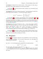
3.5.1 Computing the Probabilities . . . . . . . . . . . . . . . .
3.5.2 Static Representation of the nsDBN for Troubleshooting
3.5.3 Computing the Probabilities using the Static Representation . . . . . . . . . . . . . . . . . . . . . . . . . . . . . . .
3.6 Planner . . . . . . . . . . . . . . . . . . . . . . . . . . . . . . . . .
3.6.1 Modeling the Troubleshooting Problem as a Stochastic
Shortest Path Problem . . . . . . . . . . . . . . . . . . . .
3.6.2 Solving the SSPP . . . . . . . . . . . . . . . . . . . . . . .
3.6.3 Search Heuristics for the SSPP for Troubleshooting . . .
3.6.4 Assembly Model . . . . . . . . . . . . . . . . . . . . . . .
3.7 Relaxing the Assumptions . . . . . . . . . . . . . . . . . . . . . .
3.7.1 A Different Repair Goal . . . . . . . . . . . . . . . . . . .
3.7.2 Adapting the Heuristics . . . . . . . . . . . . . . . . . . .
3.7.3 General Feature Variables . . . . . . . . . . . . . . . . . .
3.7.4 Different Probabilistic Models . . . . . . . . . . . . . . . .
3.8 Summary . . . . . . . . . . . . . . . . . . . . . . . . . . . . . . . .
45
45
46
48
50
51
51
54
56
56
56
57
58
59
60
64
69
70
72
73
81
85
85
87
91
92
92
vii
4
Planning Algorithm
4.1 Iterative Bounding LAO* . . . . . . . . .
4.1.1 Evaluation functions . . . . . . .
4.1.2 Error Bound . . . . . . . . . . . .
4.1.3 Expanding the Fringe . . . . . .
4.1.4 Weighted Heuristics . . . . . . .
4.2 Evaluation of Iterative Bounding LAO*
4.2.1 Racetrack . . . . . . . . . . . . .
4.2.2 Rovers Domain . . . . . . . . . .
.
.
.
.
.
.
.
.
.
.
.
.
.
.
.
.
.
.
.
.
.
.
.
.
.
.
.
.
.
.
.
.
.
.
.
.
.
.
.
.
.
.
.
.
.
.
.
.
.
.
.
.
.
.
.
.
.
.
.
.
.
.
.
.
.
.
.
.
.
.
.
.
.
.
.
.
.
.
.
.
.
.
.
.
.
.
.
.
.
.
.
.
.
.
.
.
.
.
.
.
.
.
.
.
.
.
.
.
.
.
.
.
93
94
95
97
98
99
101
101
104
5
Case Study: Hydraulic Braking System
109
5.1 Introduction . . . . . . . . . . . . . . . . . . . . . . . . . . . . . . 109
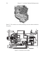
5.2 The Retarder . . . . . . . . . . . . . . . . . . . . . . . . . . . . . . 109
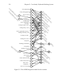
5.3 The Model . . . . . . . . . . . . . . . . . . . . . . . . . . . . . . . 111
5.4 Evaluation . . . . . . . . . . . . . . . . . . . . . . . . . . . . . . . 115
5.4.1 The Problem Set . . . . . . . . . . . . . . . . . . . . . . . . 115
5.4.2 Weighted IBLAO* vs. IBLAO* . . . . . . . . . . . . . . . 117
5.4.3 Lower Bound Heuristics . . . . . . . . . . . . . . . . . . . 120
5.4.4 Comparison with Other Algorithms . . . . . . . . . . . . 120
5.4.5 Composite Actions . . . . . . . . . . . . . . . . . . . . . . 122
5.4.6 Relaxing the Assumptions . . . . . . . . . . . . . . . . . . 122
5.4.7 Troubleshooting Performance with Limited Decision Time 127
6
Conclusion
131
Bibliography
133
A Notation
143
B Acronyms
147
C The Retarder Model File
149
viii
Part I
Introduction
1
1
Background
Troubleshooting is the process of locating the cause of a problem in a system
and resolving it. This can be particularly difficult in automotive systems such
as cars, buses, and trucks. Modern vehicles are complex products consisting of
many components that interact in intricate ways. When a fault occurs in such a
system, it may manifest itself in many different ways and a skilled mechanic is
required to find it. A modern mechanic must therefore have an understanding
of the mechanical and thermodynamic processes in for example the engine
and exhaust system as well as the electrical and logical processes in the control
units. Every year, the next generation of vehicles is more complex than the last
one, and the troubleshooting task becomes more difficult for the mechanic.
This thesis is about computer-assisted troubleshooting of automotive systems. In computer-assisted troubleshooting, the person performing the troubleshooting is assisted by a computer that recommends actions that can be
taken to locate and resolve the problem. To do this, the computer needs to be
able to reason about the object that we troubleshoot and to foresee the consequences of performed actions. Theoretical methods of doing this are developed
in this thesis. Troubleshooting heavy commercial vehicles such as trucks and
buses is of particular interest.
3
4
1.1
Chapter 1. Background
Why Computer-Assisted Troubleshooting?
The trend in the automotive industry is that vehicles are rapidly becoming
more and more complex. Increased requirements on safety and environmental
performance have led to many recent advances, especially in the engine, braking system and exhaust system [14, 70, 83]. These new systems are increasing
in complexity. For example, in addition to conventional brakes, a truck may
have an exhaust brake and a hydraulic braking system. To reduce emissions
and meet regulations, the exhaust gases can be led back through the engine for
more efficient combustion [82] or urea can be mixed with the exhaust gases to
reduce nitrogen emissions. Such systems require additional control and since
the early 1990s, the number of Electronic Control Units (ECU:s) and sensors in
vehicles has increased more than tenfold [49].
With this trend towards more complex vehicles, it is becoming more difficult, even for an experienced workshop mechanic, to have an intuitive understanding of a vehicle’s behavior. A misunderstanding of the vehicle’s behavior
can for example lead to replacing expensive ECU:s even if they are not responsible for the fault at hand. Faults may depend on a combination of electrical,
logical, mechanical, thermodynamic, and chemical processes. For example,
suppose the automatic climate control system (ACC) fails to produce the correct temperature in the cab. This can be caused by a fault in the ECU controlling
the ACC, but it can also be caused by a damaged temperature sensor used by
the ECU. The mechanic may then replace the ECU because it is quicker. However, since this is an expensive component it could be better to try replacing
the temperature sensor first. In this case, the mechanic could be helped by a
system for computer aided troubleshooting that provides decision support by
pointing out suspected faults and recommending suitable actions the mechanic
may take.
Computers are already used as tools in the service workshops. In particular, they are used to read out diagnostic messages from the ECU:s in a vehicle
and to set parameters such as fuel injection times and control strategies. The diagnostic messages, Diagnostic Trouble Codes (DTC:s), come from an On-Board
Diagnosis (OBD) system that runs on the vehicle. Ideally, each DTC points out
a component or part of the vehicle that may not function properly. However,
often it is the case that a single fault may generate multiple DTC:s and that the
same DTC can be generated by several faults. The OBD is primarily designed
to detect if a failure that is safety-critical, affects environmental performance, or
may immobilize the vehicle has occurred. This information is helpful but not
always specific enough to locate exactly which fault caused the failure. The
mechanic must therefore also gather information from other sources such as
the driver or visual inspections. In order for a computer-assisted troubleshoot-
1.2. Problem Formulation
5
ing system to be helpful for the mechanic, it must also be able to consider all
of these information sources.
Another important aspect of troubleshooting is the time required to resolve
a problem. Trucks are commercial vehicles. When they break down it is particularly important that they are back in service as soon as possible so that they
can continue to generate income for the fleet owner. Therefore, the time required to find the correct faults must be minimized. Many retailers now sell
repair and maintenance contracts which let the fleet owner pay a fixed price
for all repair and maintenance needs [45, 72, 84]. A computer-assisted troubleshooting system that could reduce the total expected cost and time of maintenance and repair would lead to large savings for the fleet owner due to time
savings and for the retailer because of reduced expenses.
1.2
Problem Formulation
We will generalize from heavy vehicles and look upon the object that we troubleshoot as a system consisting of components. Some of these components may
be faulty and should then be repaired. We do not know which components
that are faulty. However, we can make observations from which we can draw
conclusions about the status of the components. The troubleshooting task is to
make the system fault-free by performing actions on it that gather more information or make repairs. The system is said to be fault-free when none of
the components which constitute the system are faulty. We want to solve the
troubleshooting task at the smallest possible cost where the cost is measured
in time and money.
To do this, we want to use a system for computer-assisted troubleshooting,
called a troubleshooter, that receives observations from the outside world and
outputs recommendations of what actions should be performed to find and fix
the problem. The user of the troubleshooter then performs the actions on the
system that is troubleshot and returns any feedback to the troubleshooter.
The troubleshooter uses a model of the system to estimate the probability
that the system is fault-free given the available information. When this estimated probability is 1.0, the troubleshooter considers the system to be faultfree. This is the termination condition. When the termination condition holds,
the troubleshooting session is ended. The troubleshooter must generate a sequence of recommendations that eventually results in a situation where the
termination condition holds. If the troubleshooter is correct when the termination condition holds, i.e. the system really is fault-free, the troubleshooter will
be successful in solving the troubleshooting task.
When the system to troubleshoot is a truck, the user would be a mechanic.
6
Chapter 1. Background
The observations can consist of information regarding the type of the truck, operational statistics such as mileage, a problem description from the customer,
or feedback from the mechanic regarding what actions have been performed
and what has been seen. The output from the troubleshooter could consist
of requests for additional information or recommendations to perform certain
workshop tests or to replace a certain component.
1.2.1
Performance Measures
Any sequence of actions that solves the troubleshooting task does not necessarily have sufficient quality to be considered good troubleshooting. Therefore
we will need some performance measures for troubleshooting. For example,
one could make sure that the system is fault-free by replacing every single
component. While this would certainly solve the problem, doing so would be
very time-consuming and expensive.
One interesting performance measure is the cost of solving the troubleshooting task. This is the cost of repair and we will define it as the sum of the
costs of all actions performed until the termination condition holds. However,
depending on the outcome of information-gathering actions we may want
to perform different actions. The outcomes of these information-gathering
actions are not known in advance. Therefore, the expectation of the cost of repair given the currently available information is a more suitable performance
measure. This is the expected cost of repair (ECR). If the ECR is minimal, then
the average cost of using the troubleshooter is as low as possible in the long
run. Then troubleshooting is said to be optimal.
For large systems, the problem of determining what actions to perform for
optimal troubleshooting is computationally intractable [62]. Then another interesting performance measure is the time required to compute the next action
to be performed. If the next action to perform is computed while the user is
waiting, the computation time will contribute to the cost of repair. The computation time has to be traded off with the ECR because investing more time in
the computations generally leads to a reduced ECR. Being able to estimate the
quality of the current decision and give a bound on its relative cost difference
to the optimal ECR can be vital in doing this trade-off.
1.3
Solution Methods
A common approach when solving the troubleshooting task has been to divide
the problem into two parts: the diagnosis problem and the decision problem [16,
27, 33, 42, 79, 90]. First the troubleshooter finds what could possibly be wrong
1.3. Solution Methods
7
given all information currently available, and then it decides which action
should be performed next.
In Section 1.3.1, we will first present some common variants of the diagnosis problem that exist in the literature. These problems have been studied extensively in the literature and we will describe some of the more approaches.
The approaches vary in how the system is modeled and what the purpose of
the diagnosis is. In Section 1.3.2, we will present previous work on how the
decision problem can be solved.
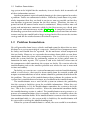
1.3.1
The Diagnosis Problem
A diagnosis is a specification of which components are faulty and non-faulty.
The diagnosis problem is the problem of finding which is the diagnosis or
which are the possible diagnoses for the system being diagnosed given the
currently available information. Diagnosis is generally based on a model that
describes the behavior of a system, where the system is seen as a set of components [7, 15, 16, 26, 33, 56, 61, 65, 77]. This can be a model of the physical
aspects of the system, where each component’s behavior is modeled explicitly
using for example universal laws of physics and wiring diagrams [7, 77]. It can
also be a black box model which is learned from training data [69, 91]. Then
no explicit representation of how the system works is required.
The purpose of diagnosis can be fault detection or fault isolation. For fault
detection, we are satisfied with being able to discriminate the case where no
component is faulty from from the case where at least one component is faulty.
Often it is important that the detection can be made as soon as possible after the
fault has occurred [35]. For fault isolation, we want to know more specifically
which diagnoses are possible. Sometimes it is not possible to isolate a single
candidate and the output from diagnosis can be all possible diagnoses [18],
a subset of the possible diagnoses [26], or a probability distribution over all
possible diagnoses [56, 81].
Consistency-Based Approach
A formal theory for consistency-based diagnosis using logical models is first
described by Reiter [61]. Each component can be in one of two or more behavioral modes of which one is nominal behavior and the others are faulty behaviors. The system model is a set of logical sentences describing how the components’ inputs and outputs relate to each other during nominal and faulty behavior. A possible diagnosis is any assignment of the components’ behavioral
modes that is consistent with the system model and the information available
in the form of observations.
8
Chapter 1. Background
The set of all possible diagnoses can be immensely large. However, it can be
characterized by a smaller set of diagnoses with minimal cardinality if faulty
behavior is unspecified [15]. If faulty behavior is modeled explicitly [18] or
if components may have more than two behavioral modes [17], all possible
diagnoses can be represented by a set of partial diagnoses.
Frameworks for diagnosis such as the General Diagnostic Engine (GDE)
[16] or Lydia [26] can compute such sets of characterizing diagnoses either
exactly or approximately. Consistency-based diagnosis using logical models
have been shown to perform well for isolating faults in static systems such as
electronic circuits [41].
Control-Theoretic Approach
In the control-theoretic approach, the system is modeled with Differential Algebraic Equations (DAE) [7, 77]. As many laws of physics can be described
using differential equations, precise physical models of dynamical systems can
be created with the DAE:s. Each DAE is associated with a component and typically the DAE:s describe the components’ behavior in the non-faulty case [7].
When the system of DAE:s is analytically redundant, i.e. there are more equations than unknowns, it is possible to extract diagnostic information [77]. If an
equation can be removed so that the DAE becomes solvable, the component to
which that equation belongs is a possible diagnosis.
These methods depend on accurate models and have been successful for
fault detection in many real world applications [36, 63]. Recently efforts have
been made to integrate methods for logical models with techniques traditionally used for fault detection in physical models [13, 44].
Data-Driven Methods
In data-driven methods, the model is learned from training data, instead of
deriving it from explicit knowledge of the system’s behavior. When large
amounts of previously classified fault cases in similar systems are available, the
data-driven methods can learn a function that maps observations to diagnoses.
Such methods include Support Vector Machines, Neural Networks, and Case
Based Reasoning (see e.g. [69], [43, 91], and [38] respectively).
Discrete Event Systems
For Discrete Event Systems (DES), the system to be diagnosed is modeled as
a set of states that the system can be in together with the possible transitions
the system can make between states. Some transitions may occur due to faults.
1.3. Solution Methods
9
An observation on a DES gives the information that a certain transition has occurred. However, not all transitions give rise to an observation. The diagnosis
task is to estimate which states the system has been in by monitoring the sequence of observations and to determine if any transitions have occurred that
are due to faults. Approaches used for DES include Petri Nets [28] and state
automata [55, 92].
Probabilistic Approaches
Probabilistic methods for diagnosis estimate the probability of a certain diagnosis being true. The model can be a pure probabilistic model such as
a Bayesian Network (BN) that describes probabilistic dependencies between
components and observations that can be made [39]. This model can for instance be derived from training data using data-driven methods [74] or from
a model of the physical aspects of the system such as bond graphs [65]. It is
also possible to combine learning techniques with the derivation of a BN from
a physical model such as a set of differential algebraic equations [56]. Once a
BN has been derived, it is possible to infer a posterior probability distribution
over possible diagnoses given the observations.
Another technique is to use a logical model and consistency-based diagnosis to first find all diagnoses that are consistent with the model and then
create the posterior distribution by assigning probabilities to the consistent diagnoses from a prior probability distribution [16]. For dynamic models where
the behavioral mode of a component may change over time, techniques such as
Kalman filters or particle filters can be used to obtain the posterior probability
distribution over possible diagnoses [5, 81]. These methods are approximate
and can often be more computationally efficient than Bayesian networks.
1.3.2
The Decision Problem
Once the troubleshooter knows which the possible diagnoses are, it should decide what to do next in order to take us closer to our goal of having all faults
repaired. Actions can be taken to repair faults or to create more observations
so that candidate diagnoses can be eliminated. There are different approaches
to deciding which of these actions should be performed. For example, one decision strategy could be to choose the action that seems to take the longest step
toward solving the troubleshooting task without considering what remains to
do to completely solve the task [16, 33, 42, 79]. Another strategy could be to
generate a complete plan for solving the task and then select the first action
in this plan [4, 89]. It is also possible to make the decision based on previous
experience of what decisions were taken in similar situations [43].
10
Chapter 1. Background
Repair B (e40)
Repair A (e90)
e130
Failure (25%)
Repair B (e40)
e140
Test system (e10)
Sys. OK (75%)
Repair A (e90)
Repair B (e40)
e100
e130
Failure (75%)
Repair A (e90)
e140
Test system (e10)
Sys. OK (25%)
e50
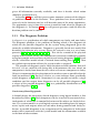
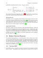
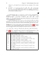
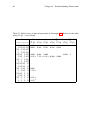
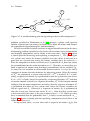
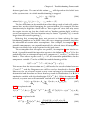
Figure 1.1: A decision tree for repairing two components A and B. Decision
nodes are shown with squares, chance nodes are shown with circles, and end
nodes are shown with triangles.
Decision Trees and Look-ahead Search
By considering every available action and every possible action outcome we
can choose an action that leads to the most desirable outcome. This can be done
using a decision tree [66]. An example of a decision tree is shown in Figure 1.1.
The decision tree has three types of nodes: decision nodes, chance nodes, and
end nodes. The nodes are joined by branches that correspond to either actions
or action outcomes. In a decision node we can choose an action to perform, and
we will follow the branch corresponding to the chosen action.. If the action
can have one of multiple outcomes we reach a chance node. Depending on
the outcome, we will follow a branch corresponding to that outcome from the
chance node to another decision node or an end node. In the end nodes the
final result is noted, e.g. "all suspected faults repaired at a cost of e130". A
decision can be made by choosing the action that leads to the most favorable
results. In the example in Figure 1.1, the most favorable decision would be to
repair component A and then proceed by testing the system. This yields a 75%
chance of a cost of e100 and a 25% chance of a cost of e140. This approach has
been used for many types of decision problems in the area of economics and
game theory [66].
For complex decision problems, though, the decision tree can become immensely large. One way to make the decision problem tractable is to prune the
tree at a certain depth k and assign each pruned branch a value from a heuristic
utility function. The decision is then the action that either minimizes or maxi-
1.3. Solution Methods
11
mizes the expected utility in k steps. This is sometimes referred to as k-depth
look-ahead search [68].
In de Kleer and Williams [16] the task is to find the fault in the system by
sequentially performing observing actions. Here the possible diagnoses are inferred from the available observations using their General Diagnostic Engine
and are assigned probabilities from a prior probability distribution as previously described in Section 1.3.1. The utility function is defined by the entropy
of the probability distribution over the possible diagnoses. In information science, the entropy of a random variable is a measure of its uncertainty [30].
Here it is used to describe the remaining uncertainty regarding which is the
true diagnosis among the set of possible diagnoses. Using only a fast onestep lookahead search, this method is remarkably efficient in finding action
sequences that find the true diagnosis at a low expected cost. Sun and Weld
[79] extend this method to also consider the cost of repairing the remaining
possible faults in addition to the entropy.
In Heckerman et al. [33] and Langseth and Jensen [42], troubleshooting of
printer systems is considered. A BN is used to model the system, the output
from the diagnosis is a probability distribution over possible diagnoses, and
the goal is to repair the system. By reducing the set of available actions and
making some rather restricting assumptions regarding the system’s behavior,
the optimal expected cost of repair can efficiently be computed analytically.
Even though these assumptions are not realistic for the printer system that
they troubleshoot, the value for the optimal ECR when the assumptions hold
is used as a utility function for a look-ahead search using the unreduced set of
actions.
Planning-Based Methods
The troubleshooting problem can be formulated as a Markov Decision Process
(MDP) or a Partially Observable MDP (POMDP) [4]. An MDP describes how
stochastic transitions between states occur under the influence of actions. A
natural way of modeling our problem is using states consisting of the diagnosis
and the observations made so far. Since we know the observations made but
do not know the diagnosis, such states are only partially observable and can
be handled using a POMDP. We can also use states consisting of a probability
distribution over possible diagnoses together with the observations made so
far. Such states are more complex, but are fully observable and allow the
troubleshooting problem to be modeled as an MDP.
A solution to an MDP or a POMDP is a function that maps states to actions
called a policy. A policy describes a plan of actions that maximizes the expected reward or minimizes the expected cost. This is a well-studied area and
12
Chapter 1. Background
there are many algorithms for solving (PO)MDP:s optimally. However, in the
general case, solving (PO)MDP:s optimally is intractable for most non-trivial
problems.
Anytime algorithms such as Learning Depth-First Search [8] or Real-Time
Dynamic Programming [2] for MDPs and, for POMDPs, Point-Based Value Iteration [59] or Heuristic Search Value Iteration [75] provide a trade-off between
computational efficiency and solution quality. These algorithms only explore
parts of the state space and converge towards optimality as more computation
time is available.
If a problem that can be modeled as a POMDP is a shortest path POMDP,
then it can be more efficiently solved using methods for ordinary MDP:s such
as RTDP rather than using methods developed for POMDP:s [10]. In a shortest
path POMDP, we want to find a policy that takes us from an initial state to a
goal.
Case Based Reasoning
In Case Based Reasoning (CBR), decisions are taken based on the observations
that have been made and decisions that have been taken previously [43]. After
successfully troubleshooting the system, information regarding the observations that were made and the repair action that resolved the problem is stored
in a case library. The next time we troubleshoot a system, the current observations are matched with similar cases in the case library [24]. If the same repair
action resolved the problem for all these cases, then this action will be taken.
Information-retrieving actions can be taken to generate additional observation
so that we can discriminate between cases for which different repairs solved
the problem. The case library can for example initially be filled with cases
from manual troubleshooting and as more cases are successfully solved the library is extended and the performance of the reasoning system improves [21].
CBR has been used successfully in several applications for troubleshooting (see
e.g. [1, 21, 29]). In these applications the problem of minimizing the expected
cost of repair is not considered and as with other data-driven methods these
methods require large amounts of training data.
1.4
Troubleshooting Framework
For the troubleshooting task, we want to minimize the expected cost of repair.
This requires that we can determine the probabilities of action outcomes and
the probability distribution over possible diagnoses. This information can
only be provided by the probabilistic methods for diagnoses. We will use a
1.4. Troubleshooting Framework
13
method for probability-based diagnosis using non-stationary Dynamic Bayesian
Networks [56]. This method is well suited for troubleshooting since it allows
us to keep track of the probability distribution over possible diagnoses when
both observations and repairs can occur.
In Section 1.3.2 we mentioned that when we know the probability distribution over possible diagnoses we can solve the decision problem using lookahead search or planning-based methods. The main advantage of the methods
that use look-ahead search is that they are computationally efficient. However,
when troubleshooting systems such as trucks, actions can take a long time for
the user to execute. With planning-based methods this time can be used more
effectively for deliberation so that a better decision can be made. We will use
a planning algorithm for MDP:s to solve the decision problem. This is because
we emphasize minimizing the expected cost of repair and that we want to be
able to use all available computation time. Modeling the problem as an MDP
works well together with a Bayesian diagnostic model.
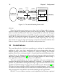
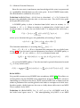
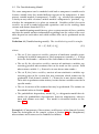
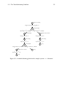
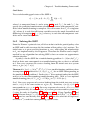
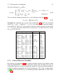
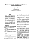
In this thesis, we have a framework for troubleshooting, where the troubleshooter consist of two parts, a Planner and a Diagnoser. The Planner and
the Diagnoser interact to produce recommendations to the user. The Diagnoser
is responsible for finding the possible diagnoses and the Planner is responsible for deciding which action should be performed next. A schematic of the
troubleshooting framework is shown in Figure 1.2.
The user informs the troubleshooter which actions have been performed on
the system and what observations have been seen. Given this information the
Troubleshooter recommends an action to perform next. The Troubleshooter
uses the Diagnoser to find out what diagnoses are possible and the Planner
to create a partial conditional plan of actions that minimizes the ECR given
the possible diagnoses. During planning, the Planner will use the Diagnoser
to estimate possible future states and the likelihoods of observations. After
planning, the Troubleshooter will recommend the user to perform the first
action in the plan created by the Planner. This could be an action that gains
more information, replaces suspected faulty components, or in some other way
affects the system.
When the Planner creates its plans, it is under time pressure. All time
that is spent computing while the user is idling contributes to the total cost
of repair. However, if the user is not ready to execute the recommended action
because the user is busy executing a previously recommended action or doing
something else, there is no loss in using this time for additional computations.
We do not know precisely how long this time can be so therefore it is desirable
that the Planner is an anytime planner, i.e. it is able to deliver a decision quickly
if needed, but if it is given more time it can plan further and make a better
14
Chapter 1. Background
System
information
User
System
information
Troubleshooter
Diagnoser
System to
troubleshoot
Possible diagnoses,
outcome likelihoods
Potential actions
Planner
Performed
actions
Recommended
actions
Figure 1.2: The troubleshooting framework.
decision.
Since the decision may improve over time, the best thing to do is not necessarily to abort the planning as soon as the user begins idling. The algorithm
that is used for the Planner in this thesis can provide the user with an upper
bound on the difference between the ECR using the current plan and the optimal ECR. The larger this bound is the greater the potential is to make a better
decision. If the user sees that the bound is steadily improving the user may
then decide to wait, in hope of receiving an improved recommendation that
leads to a lower ECR, despite the additional computation time.
1.5
Contributions
The work described in this thesis contributes to solving the troubleshooting
problem in such a way that a good trade-off between computation time and
solution quality can be made. Emphasis is placed on solving the decision
problem better than existing methods. A framework for troubleshooting is developed where the diagnosis problem is solved using non-stationary dynamic
Bayesian networks (nsDBN) [64] and the decision problem is solved using a
new algorithm called Iterative Bounding LAO* (IBLAO*).
The main contributions are the new algorithm and new and improved
heuristics for solving the decision problem by searching. The algorithm is applicable for probabilistic contingent planning in general and in this thesis it is
applied to troubleshooting of subsystems of a modern truck. Pernestål [56] has
developed a framework for nsDBN:s applied to troubleshooting. In this work,
we show how those nsDBN:s can be converted to stationary Bayesian networks
and used together with IBLAO* for troubleshooting in our application.
IBLAO* is a new efficient anytime search algorithm for creating -optimal
1.5. Contributions
15
solutions to problems formulated as Stochastic Shortest Path Problems, a subgroup of MDPs. In this thesis, we show how the troubleshooting problem can
formulated as a Stochastic Shortest Path Problem. When using IBLAO* for
solving the decision problem the user has access to and may monitor an upper
bound of the ECR for the current plan as well as a lower bound of the optimal
ECR. An advantage of this is that the user may use this information to decide
whether to use the current recommendation or to allow the search algorithm
to continue in hope of finding a better decision. As the algorithm is given more
computation time it will converge toward an optimal solution. In comparison
with competing methods, the new algorithm uses a smaller search space and
for the troubleshooting problem it can make -optimal decisions faster.
The new heuristic functions that are developed for this thesis can be used
by IBLAO*, and they provide strict lower and upper bounds of the optimal expected cost of repair that can be efficiently computed. The heuristics extend the
utility functions in [79] and [33] by taking advantage of specific characteristics
of the troubleshooting problem for heavy vehicles and similar applications.
These heuristics can be used by general optimal informed search algorithms
such as IBLAO* on the troubleshooting problem to reduce the search space
and find solutions faster than if general heuristics are used.
The new algorithm is together with the new heuristics tested on a case
study of an auxiliary hydraulic braking system of a modern truck. In the case
study, state-of-the-art methods for computer-assisted troubleshooting are compared and it is shown that the current method produces decisions of higher
quality. When the new planning algorithm is compared with other similar
state-of-the-art planning algorithms, the plans created using IBLAO* have consistently higher quality and they are created in shorter time. The case study
shows that the troubleshooting framework can be applied for troubleshooting
systems from the heavy vehicles domain.
The algorithm IBLAO* has previously been published in [87]. Parts of the
work on the heuristics have been published in [86, 88, 89]. Parts of the work
on the troubleshooting framework have been published in [58, 85, 89]. Parts of
the work on the case study have been published in [57, 89].
16
Chapter 1. Background
2
Preliminaries
This chapter is intended to introduce the reader to concepts and techniques
that are central to this thesis. In particular, different types of Bayesian networks
and Markov Decision Processes that can be used to model the troubleshooting
problem are described.
2.1
Notation
Throughout this thesis, unless stated otherwise, the notation used is as follows.
• Stochastic variables are in capital letters, e.g. X.
• The value of a stochastic variable is in small letters, e.g. X = x means that
the variable X has the value x.
• Ordered sets of stochastic variables are in capital bold font, e.g X =
{ X1 , . . . , Xn }.
• The values of an ordered set of stochastic variable is in small bold letters,
e.g. X = x means that the variables X = { X1 , . . . , Xn } have the values
x = { x 1 , . . . , x n }.
• Variables or sets of variables are sometimes indexed with time, e.g. X t =
x means that the variable X has the value x at time t and Xt = x means
that for each variable Xi ∈ X, Xit = xi . The letter t is used for discrete
17
18
Chapter 2. Preliminaries
event time that increases by 1 for each discrete event that occurs and τ is
used for real time.
• The outcome space of a stochastic variable X is denoted Ω X , i.e., the set
of all possible values the X can have. The set of all possible outcomes of
multiple variables X1 , . . . , Xn is denoted Ω( X1 , . . . , Xn ).
• The concatenation of sequences and vectors is indicated with a semicolon, e.g. ( a, b, c); (c, d, e) = ( a, b, c, c, d, e).
A list of all the notation and variable names used can be found in Appendix A
and a list of acronyms is found in Appendix B.
2.2
Bayesian Networks
This section will give a brief overview of Bayesian networks, particularly in
the context of troubleshooting. For more comprehensive work on Bayesian
networks, see e.g. Jensen [39]. We will begin by describing the basic Bayesian
network before we describe the concepts of causality and dynamic Bayesian
networks that are needed to model the troubleshooting process.
A Bayesian network (BN) is a graphical model that represents the joint
probability distribution of a set of stochastic variables X. The definition of
Bayesian networks used in this thesis follows the definition given in [40].
Definition 2.1 (Bayesian Network). A Bayesian network is a triple B = hX,E,Θi
where X is a set of stochastic variables and E is a set of directed edges between
the stochastic variables s.t. (X, E) is a directed acyclic graph. The set Θ contains
parameters that define the conditional probabilities P( X |pa( X )) where pa( X )
are the parents of X in the graph.
The joint probability distribution of all the stochastic variables X in the
Bayesian network is the product of each stochastic variable X ∈ X conditioned
on its parents:
P(X) = ∏ P( X |pa( X )).
X ∈X
Let Θ X ⊆ Θ be the parameters that define all the conditional probabilities
P( X |pa( X )) of a specific variable X. This set Θ X is called the conditional probability distribution (CPD) of X. When the variables are discrete, the CPD is called
the conditional probability table (CPT).
Bayesian networks can be used to answer queries about the probability
distribution of a variable given the value of others.
2.2. Bayesian Networks
19
Θ Xbattery
0.2
Xbattery
OK
OK
dead
dead
Xpump
OK
blocked
OK
blocked
Xbattery
Θ Xengine
0.05
1
1
1
Xpump
Θ Xpump
0.1
Xengine
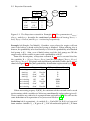
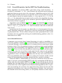
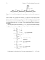
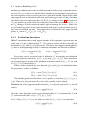
Figure 2.1: The Bayesian network in Example 2.1. The parameters Θ Xbattery ,
Θ Xpump , and Θ Xengine describe the conditional probabilities of having Xbattery =
dead, Xpump = blocked, and Xengine = notstarting respectively.
Example 2.1 (Simple Car Model). Consider a car where the engine will not
start if the battery is dead or the fuel pump is blocked. When nothing else is
known, the probability of a dead battery is 0.2 and the probability of a blocked
fuel pump is 0.1. Also, even if both battery and the fuel pump are OK the
engine may still be unable to start with a probability of 0.05.
From this description, a Bayesian network Bex2.1 can be created that has
the variables X = ( Xengine , Xbattery , Xpump ) and the two edges ( Xbattery , Xengine )
and ( Xpump , Xengine ). The graph and conditional probability tables for Bex2.1 are
shown in Figure 2.1. The joint probability distribution represented by Bex2.1 is:
Xengine
starting
starting
starting
starting
not starting
not starting
not starting
not starting
Xbattery
OK
OK
dead
dead
OK
OK
dead
dead
Xpump
OK
blocked
OK
blocked
OK
blocked
OK
blocked
P( Xengine , Xbattery , Xpump )
0.684
0
0
0
0.036
0.08
0.18
0.02
When answering a query P(X|Y), the structure of the network can be used
to determine which variables in X that are conditionally independent given Y.
These variables are said to be d-separated from each other [53]. We will use the
same definition of d-separation as in Jensen and Nielsen [40].
Definition 2.2 (d-separation). A variable Xi ∈ X of a BN hX, E, Θi is d-separated
from another variable X j ∈ X given Y ⊆ X if all undirected paths P ⊆ E from
20
Chapter 2. Preliminaries
Xi to X j are such that P contains a subset of connected edges such that:
• the edges are serial, i.e. all edges are directed the same way, and at least
one intermediate variable belongs to Y,
• the edges are diverging, i.e. the edges diverge from a variable Z in the
path, and Z ∈ Y, or
• the edges are converging, i.e. the edges meet at a variable Z in the path,
and Z ∈
/ Y.
The property of d-separation is symmetric, i.e. if Xi is d-separated from X j
given Y, then X j is d-separated from Xi given Y.
The property of d-separation is useful because it enables us to ignore the
part of the network containing X j when answering the query P( Xi |Y). Consider Example 2.1. If we have no evidence for any variable, then Xbattery is
d-separated from Xpump given Y = ∅ since the path between them is converging at Xengine and Xengine ∈
/ Y. This means that we can for example
compute P( xbattery | xpump ) simply by computing P( xbattery ). However, if we
have evidence for Xengine , then Xbattery and Xpump are not d-separated given
Y = { Xengine }. Then if we for example want to compute P( xbattery | xengine ), we
must consider Xpump :
∑ P( xengine | xbattery , xpump ) P( xbattery ) P( xpump )
xpump ∈Ω( Xpump )
.
P( xbattery | xengine ) =
0
0
0
0
)
) P( xpump
) P( xbattery
, xpump
∑ P( xengine | xbattery
0
0
xbattery
,xpump
∈Ω( Xbattery ,Xpump )
2.2.1
Causal Bayesian Networks
If there is an edge between two variables Xi and X j and the variables are such
that the value of Xi physically causes X j to have a certain value, this edge is
said to be causal [54]. E.g., a dead battery or a blocked pump causes the engine
to not start. If all edges in a BN are causal, we say that the BN is a causal
Bayesian network.
It is often easier to model a physical system with a causal BN than with a BN
that does not follow the causal relationships. The BN in Example 2.1 is causal
since having a dead battery and a blocked pump causes the engine not to start.
However, the same joint probability distribution, P( Xengine , Xbattery , Xpump ), can
be modeled with other BN:s that do not follow the causal relationships.
Example 2.2 (Non-causal Equivialent). Consider a BN Bex2.2 with same set of
stochastic variables as Bex2.1 from the previous example, but with the edges
[ Xengine , Xpump ], [ Xbattery , Xpump ] and [ Xengine , Xbattery ]. The graph and CPT:s for
Bex2.1 are shown in Figure 2.2.
2.2. Bayesian Networks
21
Θ Xengine
0.316
Xengine
Xbattery
Xengine
starting
starting
not starting
not starting
Xbattery
OK
dead
OK
dead
Θ Xpump
0
0.5
0.690
0.1
Xengine
starting
not starting
Θ Xbattery
0
0.633
Xpump
Figure 2.2: The Bayesian network in Example 2.2. The parameters Θ Xbattery ,
Θ Xpump , and Θ Xengine describe the conditional probabilities of having Xbattery =
dead, Xpump = blocked, and Xengine = not starting respectively.
The joint probability distribution represented by Bex2.2 is exactly the same
as the one represented by Bex2.1 . However, the CPT:s of Bex2.2 are less intuitive.
For example, the original model specified separate probabilities of the engine
failing to start depending on whether the battery was dead and/or the pump
was blocked. In this model, these probabilities are baked into a single unconditional probability of 3.16. That is, the pump and/or the battery are faulty
with the probability 0.28 (0.2 + 0.1 − 0.2 · 0.1) and then the engine will fail to
start with probability 1.0. If neither is faulty, the engine will fail to start with
probability 0.05, i.e. 0.316 = 0.28 · 1.0 + 0.05 · (1 − 0.28).
Interventions
An intervention is when a variable is forced to take on a certain value rather
than just being observed. If the BN is causal, we may handle interventions in
a formal way [54]. The variable that is intervened with becomes independent
of the values of its parents, e.g. if we break the engine, its status is no longer
dependent on the pump and battery since it will not start anyway. When an
intervention occurs, a new BN is created by disconnecting the intervened variable from its parents and setting it to the forced value. In the troubleshooting
scenario, interventions occur when components are repaired. Since repairs are
a natural part of the troubleshooting process we need to handle interventions
and thus use a causal Bayesian network.
Example 2.3. Consider a BN with the variables Xrain that represents whether
it has rained or not and Xgrass that represents whether the grass is wet or not.
22
Chapter 2. Preliminaries
We know that the probability for rain is 0.1 and that if it has rained the grass
will be wet and otherwise it will be dry. If we observe that it the grass is wet
we can draw the conclusion that it has rained with probability 1.0. However,
if take a hose and wet the grass we perform an intervention on the grass. Then
if we observe that the grass is wet, the probability that it has rained is still 0.1:
P( Xrain = has rained| Xgrass = wet, Xgrass := wet).
where Xgrass := wet means that the variable Xgrass is forced to take on the value
wet by an external intervention1 .
2.2.2
Dynamic Bayesian Networks
Because we perform actions on the system, troubleshooting is a stochastic
process that changes over time. Such processes can be modeled as dynamic
Bayesian networks [19].
Definition 2.3 (Dynamic Bayesian Network).
A dynamic Bayesian network
(DBN) is a Bayesian network where the set of stochastic variables can be partitioned into sets X0 , X1 , . . . where Xt describes the modeled process at the discrete time point t.
If for each variable X t ∈ Xt it is the case that pa( X t ) ⊂ nk=0 Xt−k , the DBN
is said to be an n:th order DBN. In other words, all the variables in Xt are
only dependent of the values of the variables up to n time steps earlier. The
stochastic variables Xt and the edges between them form a Bayesian network
Bt called the time slice t. The network Bt is a subgraph of the DBN.
If all time slices t > 0 are identical, the DBN is said to be stationary. A stationary first order DBN B can be fully represented by an initial BN B0 and a
transition BN B→ representing all other BN:s B1 , B2 , . . . in the DBN. The variS
ables in B→ are X t ∈Xt ({ X t } ∪ pa( X t )) for some arbitrary t > 0 and the edges
are all edges between variables in Xt and all edges from variables in pa( X t ) to
X t ∈ Xt . Often in the literature DBN:s are assumed to be first order stationary
DBN:s (see e.g. [48, 66]).
A DBN where the probabilistic dependencies change between time slices
is said to be non-stationary [64]. Non-stationary dynamic Bayesian networks
(nsDBN:s) are more general than stationary DBN:s and can handle changes
to the network that arise with interventions such as repair actions in troubleshooting.
S
1 Often, such as in the work by Pearl [54], the notation Do( X t+1 = x ) is used to describe intervention events, but it is the author’s opinion that X t+1 := x is more compact and appropriate since
the concept of intervention on a variable is similar to the assignment of a variable in programming.
2.2. Bayesian Networks
0
Xbattery
0
Xpump
0
Xengine
23
1
Xbattery
1
Xpump
1
Xengine
2
Xbattery
2
Xpump
2
Xengine
Figure 2.3: The first three time slices of Bex2.4 in Example 2.4.
Example 2.4 (Dynamic Bayesian Network). The BN Bex2.1 can be made into a
DBN Bex2.4 where the states of the battery and the pump do not change over
t−1
t
t
t−1 so
time by letting the variables Xbattery
and Xpump
depend on Xbattery
and Xpump
t−1
t−1 ) = 1. The first three time slices of B
t
t
| xpump
that P( xbattery
| xbattery
) = P( xpump
ex2.4
are shown in Figure 2.3.
If the engine is observed to not start at time 0 and we then observe that the
pump is OK at time 1 we can infer that the battery must be dead at time 2. If we
instead remove any blockage in the fuel pump at time 1 we have the knowledge
that the pump is OK, but the probability that the battery is dead at time 2 is
now 0.633, not 1.0, because the pump could still have been blocked at time 0.
1
The action of removing the blockage is an intervention on the variable Xpump
0
1
that removes the dependency between Xpump
and Xpump
. By allowing these
types of interventions Bex2.4 becomes an nsDBN.
For Example 2.4, a DBN is not really needed since the variables cannot
change values over time unless we allow interventions or we want to model
that components may break down between time slices.
2.2.3
Non-Stationary Dynamic Bayesian Networks for
Troubleshooting
In Pernestål [56] a framework for representing non-stationary dynamic
Bayesian networks in the context of troubleshooting is developed. In this
framework interventions relevant for troubleshooting are treated. The nsDBN
for troubleshooting is causal and describes the probabilistic dependencies between components and observations in a physical system. The same compact
representation of the structure with an initial BN and a transition BN that
24
Chapter 2. Preliminaries
is applicable for stationary DBN:s is not possible for general non-stationary
DBN:s. However, the nsDBN for troubleshooting can be represented by an
0 and a set of rules describing how to generate the consecutive
initial BN Bns
time slices.
Events
The nsDBN for troubleshooting is event-driven, i.e. a new time slice is generated whenever a new event has occurred. This differs from other DBN:s where
the amount of time that elapses between each time slice is static. An event can
either be an observation, a repair, or an operation of the system. If the system is a
vehicle, the operation of the system is to start the engine and drive for a certain
duration of time. After each event, a transition occurs and a new time slice is
generated. We use the notation X t+1 = x to describe the event that the variable
X is observed to have the value x at time t + 1 and X t+1 := x to describe a
repair event that causes X to have the value x at time t + 1. For the event that
the system is operated for a duration of τ time units between the time slices t
and t + 1, we use the notation ωt+1 (τ ). Note that the duration τ is a different
time measure than the one used for the time slices which is an index.
Persistent and Non-Persistent Variables
The variables in the nsDBN for troubleshooting are separated into two classes:
persistent and non-persistent. The value of a persistent variable in one time slice
is dependent on its value in the previous time slice and may only change value
due to an intervention such as a repair or the operation of the system. A component’s state is typically modeled as a persistent variable, e.g., if it is broken
at one time point it will remain so at the next unless it is repaired. A nonpersistent variable is not directly dependent on its previous value and cannot
be the parent of a persistent variable. Observations are typically modeled with
non-persistent variables, e.g. the outcome of an observation is dependent on
the status of another component.
Instant and Non-Instant Edges
The edges in an nsDBN for troubleshooting are also separated into two classes:
instant and non-instant. An instant edge always connects a parent variable to
its child within the same time slice. This means that a change in value in the
parent has an instantaneous impact on the child. An instant edge typically occurs between a variable representing the reading from a sensor and a variable
representing the measured quantity, e.g. a change in the fuel level will have an
immediate effect on the reading from the fuel level sensor.
2.2. Bayesian Networks
25
A non-instant edge connects a child variable in one time slice to a persistent
parent variable in the first time slice after the most recent operation of the
system. If no such event has occurred it connects to a persistent parent variable
in the first time slice of the network. Non-instant edges model dependencies
that are only active during operation. For example, the dependency between a
variable representing the presence of leaked out oil and a variable representing
a component that may leak oil is modeled with a non-instant edge if new oil
can only leak out when the system is pressurized during operation.
Transitions
There are three types of transitions that may occur: nominal transition, transition
after operation, and transition after repair. When an observation event has occurred the nsDBN makes a nominal transition. Then all variables X t ∈ Xt from
time slice t are copied into a new time slice t + 1 and relabeled X t+1 . For each
instant edge ( Xit , X tj ) where X tj is non-persistent, an instant edge ( Xit+1 , X tj+1 )
is added. Let tω be the time of the most recent operation event or 0 if no
such event has occurred. For each non-instant edge ( Xitω , X tj ) where X tj is nonpersistent, an edge ( Xitω , X tj+1 ) is added. For each persistent variable X t+1 , an
edge ( X t , X t+1 ) is added. In Pernestål [56] the nominal transition is referred to
as the transition after an empty event.
Transitions After Operation
When the system is operated between times t and t + 1, a transition after
operation occurs. During such a transition, persistent variables may change
values. All variables X0 and edges ( Xi0 , X 0j ) from time slice 0 are copied into
the new time slice t + 1 and labeled Xt+1 and ( Xit+1 , X tj+1 ) respectively. Also,
for each persistent variable X t+1 , an edge ( X t , X t+1 ) is added. The conditional
probability distributions of the persistent variables are updated to model the
effect of operating the system. Such a distribution can for example model
the probability that a component breaks down during operation. Then this
distribution will be dependent on the components’ state before the operation
event occurs. The distribution can also be dependent on the duration of the
operation event.
Transition After Repair
When a component variable X is repaired, a transition after repair occurs. This
transition differs from the nominal transition in that the repair is an intervention on the variable X and therefore X t+1 will have all its incoming edges re-
26
Chapter 2. Preliminaries
time slice 0
time slice 1
X61 = x6
time slice 2
X22 := x2
time slice 3
ω3 (τ )
X10
X20
X11
X21
X12
X22
X13
X23
X30
X40
X31
X41
X32
X42
X33
X43
X50
X60
X51
X61
X52
X62
X53
X63
= x6
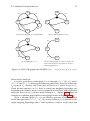
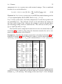
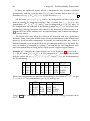
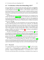
Figure 2.4: Transitions in an nsDBN.
moved. The new conditional probability distribution of X t+1 will depend on
the specific repair event. For example, it will depend on the success rate of the
repair.
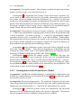
Example 2.5. Figure 2.4 shows an example of an nsDBN from time slice 0
to 3. Persistent variables are shown as shaded circles, non-persistent variables
are shown as unfilled circles, instant edges are shown as filled arrows, and
non-instant edges as dashed arrows. The first transition, after the observation
X61 = x6 , is nominal. The second transition is after the intervention X22 := x2
and the third is after operation. After the operation, the time slice looks the
same as in the first time slice. If, instead of ω3 (τ ), we would have observed
the variable X6 again, this variable would have a value that is dependent on
X20 before the intervention.
Parameters
The parameters required for the nsDBN for troubleshooting describe the dependencies within the first time slice, Θ0X , and the dependencies between persistent variables and their copies in the next time slice after a transition after
operation, Θω
X . For subsequent time slices these parameters are reused, e.g. in
2.2. Bayesian Networks
27
time slice 2 of Example 2.5, P( X32 | X10 , X22 ) = Θ0X3 ( X1 , X2 ).
Definition 2.4 (nsDBN). An nsDBN is a tuple Bns = hXp , Xnp , Ei , Eni , Θ0 , Θω i
where Xp are the persistent variables, Xnp are the non-persistent variables, and
Ei and Eni are the instant edges and non-instant edges in the first time slice
respectively. The parameters Θ0 specify the conditional probability distributions for all variables in the first time slice so that hXp ∪ Xnp , Ei ∪ Eni , Θ0 i is an
ordinary BN. The parameters Θω specify the conditional probabilities for the
transitions after operation.
Let Bns be an nsDBN and let e1:t be a sequence of events that has occurred,
then Bns (e1:t ) is the Bayesian network that is obtained by adding new time
slices to the nsDBN using the corresponding transition rule for each event in
e1:t .
2.2.4
Inference in Bayesian Networks
The process of answering a query P(X|Y) is called inference. The probability
distribution over X is inferred from the BN model given the evidence Y. The
inference can be exact or approximate. For general discrete Bayesian networks,
the time and space complexity of exact inference is exponential in the size of the
network, i.e., the number of entries in the conditional probability tables [66].
In this section, we will describe the most basic methods for making inference
in BN:s.
Variable Elimination Algorithm
Variable Elimination [66] is an algorithm for exact inference in BN:s. Other
algorithms in the same family include Bucket Elimination [20] and Symbolic
Probabilistic Inference [73].
Let hX, E, Θi be a BN where the variables X = ( X0 , . . . , Xn ) are ordered so
that Xi ∈
/ pa( X j ) if j < i and let Y ⊆ X be the set of variables we want to obtain
a joint probability distribution over. Further, let Yi+ = Y ∩
n
S
k =i
Xk be the set of
variables in Y that have the position i or greater in X, and let Xi− =
i−
S1
k=0
Xk be
the set of variables in X that have the position i − 1 or less in X. Then the joint
28
Chapter 2. Preliminaries
−
probability distribution over Y, P(y) = P(y+
0 |x0 ) where
P(yi+ |xi− ) =


P( yi |xi− )




1
if i = n and Xi ∈ Y,
P( yi |xi− ) P(yi++1 |xi− ∪ xi )





 ∑ P( xi |xi− ) P(yi++1 |xi− ∪ yi )
xi ∈ Xi
if i < n and Xi ∈ Y,
if i = n and Xi ∈
/ Y,
(2.1)
if i < n and Xi ∈
/ Y.
The Variable Elimination algorithm solves (2.1) using dynamic programming
so that the results of repeated calculations are saved for later use.
Message-Passing
If the BN is a tree it is possible to do inference in time linear in the size of the
network by using the method of message passing [51]. The size of the network
again refers to the number of entries in the conditional probability tables. A
general BN can be converted into a tree, but in the worst case, this operation
may cause the network to grow exponentially [52].
Approximate Methods
If the BN is large it may be necessary to do approximate inference. Many of
the methods for approximate inference depend on some randomization process such as sampling from the prior distribution and give each sample some
weight based on their importance to explaining the evidence. These kinds of
methods are often used for DBN:s in real-time applications such as robotics
(see e.g. Thrun et al. [80]).
2.3
Markov Decision Processes
The troubleshooting problem is a decision process where actions may be chosen freely by the decision maker to achieve the goal of repairing the system but
the actions may have stochastic outcomes. Markov Decision Processes (MDP:s)
provide a powerful mathematical tool to model this. This section gives a brief
overview of some types of MDP:s that are relevant for this thesis. For more
information on MDP:s, see e.g. [60].
2.3.1
The Basic MDP
In an MDP, a state is a situation in which a decision of what action to perform
must be made. Depending on the action and the outcome of the action, a
2.3. Markov Decision Processes
29
different state may be reached. Depending on the decision and the state where
the decision is made an immediate positive or negative reward is given. The
goal is to find a decision rule that maximizes the expected total reward over a
sequence of actions.
Definition 2.5 (Markov Decision Process). A Markov Decision Process is a tuple
hS , A, p, ri
where S is a state space, A is a set of possible actions, p : S 2 × A 7→ [0, 1] is a
R
transition probability function where ∀ s ∈ S , a ∈ A s0 ∈S p(s0 , s, a)ds0 = 1, and
r : A × S 7→ R is a reward function.
In the general case, the state space and the set of possible actions may be
continuous, but for the application of MDP:s used in this thesis, we will only
consider MDP:s where the set of possible actions is discrete and finite.
The value p(s0 , s, a) specifies the probability that the state s0 is reached given
that the action a is performed in state s. Each state that can be reached with a
non-zero probability corresponds to one possible outcome of the action. We
will assume that each action will only have a finite number of outcomes in any
state. Those states that have non-zero probability of being reached are specified
by the the successor function.
Definition 2.6 (Successor function). The successor function is a function succ :
A × S 7→ 2S such that succ( a, s) = {s0 ∈ S : p(s0 , s, a) > 0}.
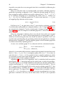
A graphical representation of a small discrete MDP with two states and
two actions is shown in Figure 2.5. The states are shown as nodes and state
transitions as edges. State transitions that correspond to the same action being
performed in the same state but with different possible outcomes, are shown
joined with an arc.
Policies
A decision rule for an MDP is called a policy. A policy is a function π : S 7→ A
where π (s) specifies which action that should be performed in state s. This
means that the policy indirectly specifies action plans that are dependent on
actual action outcomes and can result in an infinite number of actions being
performed. The quality of such a policy can be measured using the total expected discounted reward criterion. The total expected discounted reward of a
policy π is given by a function Vπγ : S 7→ R where γ ∈ [0, 1] is a discount factor
and
Vπγ (s) = r(π (s), s) + γ ∑ p(s0, s, π (s))Vπγ (s0 ).
(2.2)
s0 ∈succ(π (s),s)
30
Chapter 2. Preliminaries
p(s1 , s1 , a1 ) = 0.5
p(s2 , s2 , a1 ) = 1
r( a1 , s2 ) = 1
p(s2 , s1 , a1 ) = 0.5
r( a1 , s1 ) = 5
s1
s2
r( a2 , s2 ) = −1
p(s1 , s2 , a2 ) = 0.5
p(s1 , s1 , a2 ) = 1
r( a2 , s1 ) = −2
p(s2 , s2 , a2 ) = 0.5
Figure 2.5: An example of a small discrete MDP h{s1 , s2 }, { a1 , a2 }, p, ri.
The discount factor γ enables us to value future rewards less than immediate
rewards. When the discount factor is 1.0 then (2.2) is the expectation of the total
accumulated reward gained from using the decision rule over an infinitely long
period of time. This would mean that the reward can be infinite, but if γ < 1
and all rewards are finite, then Vπγ (s) < ∞ for all policies π and all states s.
An optimal policy π ∗ has the maximal expected discounted reward Vπγ∗ in
all states s:
π ∗ (s) = arg max r( a, s) + γ ∑ p(s0, s, a)Vπγ∗ (s0 ) .
(2.3)
a∈A
2.3.2
s0 ∈succ( a,s)
Partial Observability
In troubleshooting, the state of the system can for example be its true diagnosis,
i.e., the status of all components. The true diagnosis is however not known, but
we can get feed-back in the form of observations that can give us information
of which diagnoses are likely to be true. Such a state is said to be partially
observable. An MDP with partially observable states is a Partially Observable
MDP (POMDP) [12].
Definition 2.7 (Partially Observable MDP). A Partially Observable MDP is a
tuple
hS , A, O , r, p, ωi
where S and A are finite, hS , A, r, pi is an MDP, O is a set of possible observations and ω : O × S × A 7→ [0, 1] is a function where ω(o, s, a) is the
probability of making the observation o ∈ O given that action a is performed
in state s.
2.3. Markov Decision Processes
31
Since the true state is not known, our knowledge of this state is represented
as a probability distribution over the state space. In the POMDP framework,
this distribution is called the belief state b.
Definition 2.8 (Belief State). A belief state is a function b : S 7→ [0, 1] where b(s)
denotes the probability that the state s is the true state. The set B is the space
of all possible belief states.
A POMDP policy is then a function from belief states to actions, i.e. a
function π : B 7→ A. When an action a is performed in a belief state b and
an observation o is made, the next belief state b0 is computed for each state s,
as [12]:
.
b0 (s) = ω(o, s, a) ∑ p(s0, s, a)b(s0 ) η(o, b, a)
(2.4)
s0 ∈succ( a,s)
where η is a function that gives the probability of reaching b0 from b:
η(o, b, a) = ∑ ω(o, s, a) ∑ p(s0, s, a)b(s0 )
s∈S
s0 ∈succ( a,s)
This function normalizes b0 ensuring that ∑s∈S b0 (s) = 1.
Let τ : O × B × A 7→ B be a function that computes the next belief state
using (2.4). Then the total expected discounted reward of a POMDP policy π
is a function Vπγ : B 7→ R where γ ∈ [0, 1] is a discount factor and
Vπγ (b) =
∑ b ( s )r ( π ( b ) , s ) + γ ∑
s∈S
η(o, b, a)Vπγ (τ (o, b, a)).
(2.5)
o∈O
An optimal POMDP policy π ∗ has the maximal expected discounted reward
in every belief state b:
Vπγ∗
π ∗ (b) = arg max
a∈A
∑ b ( s )r ( π ( b ) , s ) + γ ∑
s∈S
η(o, b, a)Vπγ (τ (o, b, a)) .
(2.6)
o∈O
Belief-MDP:s
It is possible to convert any POMDP into an ordinary MDP [12]. This allows us
to find policies for the POMDP using algorithms designed for MDP:s which is
something we will do in this thesis. If the current belief state is known and an
action is performed the resulting belief state leads to a unique next belief state.
In other words, a belief state can be seen as a fully observable state in an MDP.
This is called a belief-MDP.
Definition 2.9 (Belief-MDP). Let hS , A, O , r, p, ωi be a POMDP and B be
the belief state space over S . The corresponding belief-MDP is an MDP
32
Chapter 2. Preliminaries
hS 0 , A0 , r0 , p0 i where the state space S 0 = B is the belief state space
of the POMDP, the set of possible actions A0 = A remains the same,
r0 ( a, b) = ∑s∈S b(s)r( a, s) is the expected reward of performing a in b,
and p0 (b0 , b, a) = η(o, b, a) is the probability of reaching the belief state b0
by performing a in the belief state b where o is an observation such that
τ (o, b, a) = b0 .
2.3.3
Stochastic Shortest Path Problems
A stochastic shortest path problem (SSPP) is a problem that can be modeled
with an MDP where we want to reach one of a set of goal states from a given
initial state [6]. Performing an action is associated with a cost and the actions
may have stochastic outcomes. An SSPP can be used to encode many problems
where a plan of actions leading to a goal state is sought. One such problem
is the problem of computer-assisted troubleshooting. SSPP:s correspond to
MDP:s where all rewards are non-positive, and some states are absorbing, i.e.
the reward for performing any action in an absorbing state is zero and we will
end up in the same state with probability 1.0.
The absorbing states are the goal states that we want to reach and the nonpositive reward function encodes the cost of performing actions in each state.
For simplicity, we will model the cost of performing actions directly with a cost
function.
Definition 2.10 (Cost Function). The cost function is a function c : S × A 7→ R+
such that c( a, s) is the cost of performing the action a in the state s.
Definition 2.11 (Stochastic Shortest Path Problem). A Stochastic Shortest Path
Problem is a tuple
hS , A, p, c, s0 , S g i
where hS , A, p, −ci is an MDP, s0 is the initial state, and S g is the set of absorbing goal states. All states s ∈ S g are such that, for all actions a ∈ A,
p(s, s, a) = 1 and c( a, s) = 0. All other states s ∈
/ S g are such that, for all
actions a ∈ A, c( a, s) > 0.
A policy for an SSPP is a policy for the corresponding MDP. Therefore and
because the cost function is the negative reward function of the corresponding
MDP, the expected cost of a policy π of an SSPP is a function defined as Vπ =
−Vπγ where γ = 1. An optimal policy π ∗ has minimal expected cost in all states
s:
Vπ ∗ (s) = min r( a, s) + ∑ p(s0, s, a)Vπ ∗ (s0 ).
(2.7)
a∈A
s0 ∈succ( a,s)
2.3. Markov Decision Processes
33
Since the SSPP has absorbing goal states, it may be possible to find a policy that can reach a goal state from the initial state with a finite expected cost
since in the absorbing states all infinite sequences of actions will have an expected cost that is zero. Such a policy exists if all action costs are finite and
if by following the policy from the initial state, a goal state will eventually be
reached.
2.3.4
Finding the Optimal Policy for an MDP
In this section we will go through some methods for finding optimal or suboptimal policies for the different types of MDP:s described in Sections 2.3.1–2.3.3.
Value Iteration
Value Iteration [3] is a standard method for finding near optimal policies for
ordinary MDP:s with discrete state spaces. When the discount factor γ < 1,
Value Iteration can find a policy π where Vπγ∗ (s) − Vπγ (s) < in all states s for
an arbitrary small ε > 0 . The Value Iteration algorithm is shown below as
Algorithm 1.
A function f : S 7→ R called the value function approximates the expected
reward of the policy π that is returned from the algorithm. The value function
holds a value for each state and each value is initialized with an arbitrary initial
guess as given by the function h : S 7→ R. In each iteration through the lines
5–10, the values in f will converge further toward the optimal expected reward
function Vπγ∗ . The operation in line 7 of updating the value of f for a state s is
called a backup of state s. In line 12 a policy π is created that is greedy in the
value function. Clearly, if f (s) = Vπγ∗ (s) for all s ∈ S , then line 12 is the same
as (2.3) and π is optimal. When the largest change ∆ in the value function for
any state after an iteration is smaller than ε(1 − γ )/2γ, then it can be shown
that Vπγ∗ (s) − Vπγ (s) < ε for all states s [60].
The closer the initial guess is to real optimal expected cost, the faster Value
Iteration will converge. The states are backed up an equal number of times. Depending on the order in which the states are backed up, convergence toward
an optimal policy can be faster or slower. It is possible to construct algorithms
that are similar to Value Iteration and that back up certain states in the value
function more often than other states. To guarantee that the value function
converges toward the optimal expected reward, it is sufficient that the probability that each state will be backed up infinitely often is 1.0 during an infinite
sequence of backups. This means that all states must have a non-zero probability of being backed up.
34
Chapter 2. Preliminaries
Algorithm 1 Value Iteration
1: procedure VALUE I TERATION (MDP,γ,ε,h)
2:
for each s ∈ S do f (s) ← h(s)
3:
∆←∞
4:
while ∆ ≥ ε(1 − γ )/2γ do
5:
∆←0
6:
for each s ∈ S do
7:
p ← max a∈A r( a, s) + ∑s0 ∈succ(a,s) p(s0 , a, s) f (s)
8:
∆ ← max(∆, | f (s) − p|)
9:
f (s) ← p
10:
end for
11:
end while
12:
for each s ∈ S do π (s) ← arg max a∈A r( a, s) + ∑s0 ∈succ(a,s) p(s0 , a, s) f (s)
13:
return π
14: end procedure
Real Time Dynamic Programming
Real Time Dynamic Programming (RTDP) is an algorithm for finding nearoptimal policies for SSPP:s [2].
For SSPP:s convergence can be achieved without backing up all states. The
value function will converge toward the optimal expected cost for all states
reachable from the initial state under the optimal policy if the following conditions holds [2]:
• the value function is initialized to some value strictly lower than the
optimal expected cost, and
• any state, that is reachable from the initial state using the policy that
is greedy on the current value function, is backed up with a non-zero
probability.
Consider an SSPP hS , A, p, c, s0 , S g i. For any action a ∈ A, let Ta be an
operator on functions f : S 7→ R such that for any state s
Ta f (s) = c( a, s) +
∑
p(s0 , s, a) f (s0 ).
s0 ∈succ( a,s)
The RTDP algorithm explores the state space randomly through a series
of trials, depth first random walks starting from the initial state. The RTDP
algorithm is shown below as Algorithm 2. As input it is given an SSPP, a
heuristic function h : S 7→ R+ that gives an estimate of the optimal expected
cost for every state s ∈ S such that h(s) ≤ Vπ ∗ (s), a time limit Tstop that
2.3. Markov Decision Processes
35
specifies when the algorithm should halt, and a time limit Ttrial that specifies
the maximum duration of each trial.
The current policy π is undefined for states that have not been backed
up. The trials (lines 10–16) are run repeatedly until the algorithm times out
when CPU_time − t0 ≥ Tstop starting from the initial state s0 . If a state s is
encountered and s has not been expanded before, then s is expanded at line 11.
That is, all successor states s0 are generated for all actions and s is inserted into
the set G and the value function is set according to the heuristic f (s0 ) = h(s0 ).
Every encountered state s is first backed up, i.e. the current policy for that
state π (s) is selected and value function f (s) is updated. Then a successor state
s0 ∈ succ(π (s), s) is drawn randomly from the distribution p(·, s, π (s)) (line 13)
and the trial continues from s0 through a recursive call to RUN T RIAL (line 14).
If a goal state is reached or the time limit Ttrial is reached, RTDP backtracks and
backs up all the encountered states again in reverse order.
The algorithm stops when the time limit Tstop is reached. RTDP is guaranteed to converge toward an optimal policy as Tstop → ∞. However, when
the algorithm stops we cannot tell how close the expected cost of the obtained
policy will be to the optimal expected cost.
RTDP does not need to explore every state in the state space and will therefore work even if the state space is infinite. It is sufficient that the number of
actions and action outcomes in each state are finite, which is the case in a beliefMDP. Since the trials originate from the initial state s0 , the quality of the policy
will tend to improve faster there. Therefore RTDP can be used as an anytime
algorithm when computation time is limited [2].
LAO*
LAO* [31] is an algorithm for finding solutions in cyclic AND/OR graphs
and it can also be used to find near-optimal policies for SSPP:s. LAO* is an
extension of AO* [50], a search algorithm for acyclic AND/OR graphs. This
algorithm will be the basis for the new algorithm Iterative Bounding LAO*
that is one of the contributions of this thesis (Chapter 4). We will therefore go
through this algorithm in detail.
The search graph for LAO* is an AND/OR graph which can be represented as a directed hypergraph where the nodes are states and the edges
correspond to actions. We can create such a graph G = (N , E ) for an SSPP
hS , A, p, c, s0 , S g i as follows. Let s0 belong to N and for every state s ∈ N \ S g
and every action a ∈ A, let the states in succ( a, s) also belong to N . Also, add
to E one outgoing edge (s, succ(s, a)) that leads from s to the states in succ(s, a).
This results in a graph where all leaves are goal states. Figure 2.6(a) shows an
example of such an AND/OR graph. The hyperedges are shown as arrows
36
Chapter 2. Preliminaries
Algorithm 2 Real Time Dynamic Programming
1: procedure RTDP(SSPP,h,Tstop ,Ttrial )
2:
G←∅
3:
f (s0 ) ← h(s0 )
4:
t0 ← CPU_time
5:
while CPU_time − t0 < Tstop do
6:
RUN T RIAL (s0 , CPU_time)
7:
end while
8:
return π
9: end procedure
10:
11:
12:
13:
14:
15:
16:
17:
18:
19:
20:
21:
22:
23:
24:
procedure RUN T RIAL(s,t)
if s ∈
/ G then EXPAND(s)
DO B ACK U P (s )
s0 ← s0 ∼ p(·, s, π (s))
if s0 ∈
/ S g ∧ CPU_time − t < Ttrial then RUN T RIAL (s0 , t0 )
DO B ACK U P (s )
end procedure
procedure EXPAND(s)
G ← G ∪ {s}
for each a ∈ A, s0 ∈ succ( a, s) do f (s0 ) ← h(s0 )
end procedure
procedure DO B ACK U P(s)
f (s) = min a∈A Ta f (s)
π (s) = arg min a∈A Ta f (s)
end procedure
2.3. Markov Decision Processes
s0
a1
37
s0
a1
a2
s1
a1
a2
s2
s1
s2
a2
a2
a2
a1
s3
s3
(a) The search graph G of a small SSPP.
s0
a1
(b) A solution graph Gπ for G.
a1
s0
a2
s1
s2
s1
a2
a1
s3
(c) A subgraph G 0 ⊂ G.
a1
s3
(d) A solution graph Gπ0 fpor G 0 where all
leaves are also leaves in G thus Gπ0 is also a
solution graph for G.
Figure 2.6: AND/OR graphs for the SSPP h{s0 , . . . , s3 }, { a1 , a2 }, p, c, s0 , {s3 }i
.
joined with a small arc.
A solution graph for a search graph G is a subgraph Gπ = (Nπ , Eπ ) where
Nπ ⊆ N and Eπ ⊆ E satisfying the following constraint. First, the initial state
s0 is part of Gπ . Second, only states that are leaves in G can be leaves in Gπ .
Third, for any non-leaf s in Gπ , there is exactly one outgoing hyperedge corresponding to a chosen action a to be performed in that state, and all possible
successor states succ( a, s) of that action belong to Gπ . Figure 2.6(b) shows an
example of a solution graph for the search graph shown in Figure 2.6(a).
Given a solution graph Gπ , we can directly generate a policy π where
for all non-goal states s ∈ Gπ \ S g , the chosen action π (s) is defined by the
single outgoing hyperedge from s. Such a policy is complete, in the sense that
38
Chapter 2. Preliminaries
it specifies an action for every non-goal state that is reachable by following the
policy within G.
Now we will show how we incrementally can build a solution graph by
gradually expanding a subgraph G 0 of G. From this solution graph we can extract a complete policy without necessarily explore all of G. Let G 0 = (E 0 , N 0 )
be an arbitrary subgraph of G containing the initial state s0 . Further, let
Gπ0 = (Eπ0 , Nπ0 ) be a solution graph for G 0 where each non-leaf s ∈ Gπ0 has
an outgoing edge labeled with an action
π (s) = arg min Ta f (s).
(2.8)
a∈A
If all leaves in Gπ0 are goal states, then Gπ0 must also be a solution graph for
G and therefore corresponds to a complete policy π for G. Figure 2.6(c) shows
an example of a subgraph G 0 to the search graph G shown in Figure 2.6(a) and
Figure 2.6(d) shows an example of a solution graph for G 0 that is also a solution
graph for G.
Since the subgraph is arbitrary, there may also be leaves that are not goal
states. In this case, Gπ0 can be said to correspond to a partial policy π for G,
which can lead to non-goal states for which no action is specified. LAO* can
expand such a partial policy by specifying actions for non-goal leaves, thereby
incrementally expanding G 0 until its solution graph is also a solution graph for
G without necessarily exploring all of G.
A state s in a solution graph Gπ0 is evaluated with the evaluation function
(
f (s) =
h(s)
if s is a leaf state in G 0 ,
Tπ (s) f (s)
otherwise,
(2.9)
where h(s) is an admissible heuristic estimate of the optimal expected cost such
that 0 ≤ h(s) ≤ Vπ ∗ (s). If π is a complete policy then f (s) = Vπ (s) since in
each leaf, h(s) = Vπ (s) = 0. It is possible to have complete policies in which
it is possible to reach states from which a goal state is unreachable. However,
the expected cost of such a policy is infinite.
Algorithm 3 shows the LAO* algorithm. LAO* is initialized with an explicit
search graph G 0 ⊆ G consisting only of the initial state s0 and no hyperedges.
The current policy π is initially undefined, therefore the solution graph of the
explicit search graph Gπ0 = (Nπ0 , Eπ0 ) consists only of the leaf state s0 . The set
Φ( Gπ0 ) consists of all non-goal leaves in the current solution graph of G 0 that
are reachable from s0 . Initially, Φ( Gπ0 ) = {s0 } unless the initial state happens
to be a goal state. The loop in lines 4–11 will ensure that eventually in G 0 , the
set Φ( Gπ0 ) = ∅, i.e. that there is eventually an action to perform for every nongoal state. Until this is the case, one or more states s in Φ( Gπ0 ) are expanded
2.3. Markov Decision Processes
39
(lines 5–9). Then for all actions a ∈ A, the successor states succ(s, a) and the
corresponding hyperedges (s, succ( a, s)) are added to G 0 .
Algorithm 3 LAO*
1: procedure LAO*(SSPP = hS , A, p, c, s0 , S g i,ε,h)
2:
G 0 = (N 0 , E 0 ) ← ({s0 }, ∅)
3:
f (s0 ) ← h(s0 )
4:
while Φ( Gπ0 ) 6= ∅ do
5:
Sexpand ← ∅
6:
for some s ∈ Φ( Gπ0 ) do
7:
Sexpand ← Sexpand ∪ {s}
8:
EXPAND (s )
9:
end for
10:
VALUE I TERATION (hSexpand ∪ ancestors(Sexpand ), A, pi, 1.0, ε, f )
11:
end while
12:
VALUE I TERATION (h{s : s ∈ Gπ0 }, A, pi, 1.0, ε, f )
13:
if Φ( Gπ0 ) 6= ∅ then goto line 4.
14:
return π
15: end procedure
16:
17:
18:
19:
20:
21:
22:
23:
24:
procedure EXPAND(s)
for each a ∈ A do
for each s0 ∈ succ( a, s) \ N 0 do
f (s0 ) = h(s0 )
end for
N 0 ← N 0 ∪ succ( a, s)
E 0 ← E 0 ∪ (s, succ( a, s))
end for
end procedure
After the expansions, (2.9) is evaluated for all the newly expanded states in
Sexpand and their ancestors(Sexpand ) using the Value Iteration algorithm in line
10. Value Iteration updates both the value function f and the current policy π
for these states.
When Φ( Gπ0 ) = ∅, then in line 12 LAO* performs value iteration again, this
time over all states in Nπ0 until either the f -values converge or some non-goal
state appears among the leaf states of Gπ0 in which case LAO* goes back to
line 4. When all leaves in Gπ0 are goal states and the f -values have properly
converged by Value Iteration, Φ( Gπ0 ) = ∅ and Vπ − Vπ ∗ < in line 14.
40
2.3.5
Chapter 2. Preliminaries
Finding the Optimal Policy for a POMDP
Finding an optimal policy for a POMDP is much more difficult than for an
MDP with a finite state space of equal size. However, in certain situations a
POMDP may be solved more efficiently than the corresponding belief-MDP
which has a much larger state space.
If we are interested in finding plans with a fixed depth T, the value function
(2.5) of an optimal policy can be represented by a piecewise linear function.
This is used by several POMDP algorithms. Instead of representing the optimal value function as a vector over states, the optimal T-step policy is represented with a set of linear constraints Υ T on the belief space B . Each constraint
is a pair h a, VT i where a is the first action of some T-step policy and VT is a
vector specifying the expected reward of that policy for each state s ∈ S . The
optimal T-step policy is extracted from Υ T as
π T∗ (b) = arg max
∑ b(s)VT (s).
h a,VT i∈Υ T s∈S
Initially the set of constraints Υ1 consists of one constraint h a, V1 i for every
action a ∈ A where V1 (s) = r( a, s) for every state s ∈ A. We can compute the
next set of constraint Υ T +1 from a previous set of constraints Υ T and thereby
obtain optimal policies of any length. Let VT be a function O 7→ Υ T , and let
ΩVT be the set of all possible such functions. The next set of constraints Υ T +1
can then be obtained from the previous one by adding a constraint h a, VT +1 i
for every a ∈ A and every VT ∈ ΩVT where
VT +1 (s) = r( a, s) + γ
∑
ω(o, s, a)
∑
0
o∈O
p(s0 , s, a)VT (o)(s0 ) .
s ∈succ( a,s)
By letting T → ∞ the expected reward for an optimal infinite horizon
POMDP policy can be approximated with arbitrary precision. If this is done
|O| T −1
naively, the size of Υ T would be |A| |O|−1 . However, not every constraint in
Υ T is needed. Every constraints that is dominated by some other constraint in
each point in b ∈ B can be removed.
State of the art POMDP solvers vary in the way in which they remove constraints from Υ T . For example, Point-Based Value Iteration (PBVI) [59] removes
all constraints that are dominated by some other constraint in a limited set of
belief states in the belief space. This is an approximation because a removed
constraint could be the dominating constraint in belief states outside this limited set of belief states.
Another algorithm, Heuristic Search Value Iteration (HSVI) [75], removes
only those constraints that are point-wise dominated by some other constraint.
2.3. Markov Decision Processes
41
This guarantees that no constraint from the optimal set of constraints is removed.
42
Chapter 2. Preliminaries
Part II
Decision-Theoretic
Troubleshooting of Heavy
Vehicles
43
3
Troubleshooting Framework
This chapter is on the framework for troubleshooting described in Section 1.4.
We will formally define the troubleshooting model and the troubleshooting
problem in Sections 3.2 and 3.3. We will also define a set of assumptions that
can be applied when modeling the troubleshooting process for heavy vehicles
in Section 3.4. When describing the Diagnoser in Section 3.5 we will present a
new way to represent and use the non-stationary Dynamic Bayesian Networks
for troubleshooting. In Section 3.6 we present the Planner. There we will show
how the troubleshooting problem can be modeled and solved as a Stochastic
Shortest Path Problem (SSPP). Many solvers for SSPP:s benefit from using
search heuristics. New heuristics applicable for the troubleshooting problem
are presented in Section 3.6.3. In Section 3.6.4 we will show how certain actions
can grouped together to make the planning process more efficient without
losing optimality. In Section 3.7 we will study what the consequences will
be if we relax some of the assumptions previously made in Section 3.4, thus
creating a more general framework.
3.1
Small Example
Here we will introduce a small sample system that is used to demonstrate some
of the concepts of the modeling, inference and planning in the troubleshooting
framework. The example will be incrementally expanded as more concepts are
45
46
Chapter 3. Troubleshooting Framework
Pressure
Oil Level
Oil
Pump
Leakage
Gasket
Figure 3.1: Schematic of example system.
introduced.
In the sample system (Figure 3.1), oil is pumped through a pipe connected
to a smaller pipe through a gasket. The system includes an oil pressure sensor
and a dipstick to check the oil level. There are four different faults which may
cause the system to fail. In case of a pump failure, nominal pressure cannot be
maintained. This will also happen if the oil level is too low. In case of a leaking
gasket, the oil level will fall. However the oil level can also be low for other
unknown reasons. Leaking oil from a faulty gasket may or may not be visible
on the outside of the pipe. When the pressure is low, a low pressure alarm is
raised. This alarm will also be triggered in case of a fault in the pressure sensor.
A mechanic that is troubleshooting this system may repair the system by refilling the oil, repairing the oil pump, or replacing the gasket or the oil pressure
sensor. Also, the mechanic may gain additional information of the system by
observing the oil level, searching for a visible leakage or inspecting the pump.
To reach the pipe an outer protective casing must be removed. This must be
done before performing any action on the pump or gasket. Also, to replace the
gasket the smaller pipe must be removed. To test the system and see if a low
pressure alarm is triggered the entire system must be assembled.
3.2
The Troubleshooting Model
Parts of the system that may fail, i.e., components such as sensors, actuators,
wiring, and pipes, are modeled with variables called component variables. Parts
of the system that may affect when an action can be performed, such as the
protective casings around components that must be removed before certain
actions can be performed, are modeled with variables called feature variables.
3.2. The Troubleshooting Model
47
The same component can be modeled with both a component variable and a
feature variable since they model different aspects of the component. A component variable models a component’s "health", e.g., whether the component
is faulty or not, while a feature variable models a component’s "position", e.g.,
whether the component is in place or removed. Variables called observation
variables are used to model observable quantities such as the readings from
sensors and alarms from the ECU:s.
The troubleshooting model for any given system consists of these variables
and also the model contains information regarding how the values of the variables depend on each other and which actions that can be performed on the
system.
Definition 3.1 (Troubleshooting model). The troubleshooting model is a tuple
M = hC, O, F, A, MP i
(3.1)
where:
• The set C, the component variables, consists of stochastic variables representing the health of components. Each component variable C ∈ C must
be in one fault mode c. and one of the fault modes is the no fault case NF.
• The set O, the observation variables, consists of stochastic variables representing possible observations that can be made on the system. Each
observation variable O ∈ O must be in one observation mode o.
• The set F, the feature variables, consists of non-stochastic variables representing parts of the system that may constrain which actions can be
performed. Each feature variable F ∈ F must be in one feature mode f .
To be able to perform certain actions, certain feature variables must be in
specific modes.
• The set A consists of the actions that may be performed. The actions are
described further in Section 3.2.1.
• The probabilistic dependency model MP is a diagnostic model that describes the probabilistic dependencies between components, observations and actions over time. This model is described further in Section 3.2.2.
Example 3.1 (Components, Observations, and Features of the Sample System).
From the description of the sample system in Section 3.1, the components,
observations and features can be modeled as follows:
48
Chapter 3. Troubleshooting Framework
Variable
C1 Pump
C2 Gasket
C3 Pressure Sensor
C4 Oil Level
O1 Visible Leakage
O2 Low Oil Pressure
O3 Low Oil Pressure Alarm
F1
Outer Casing
F2
Small Pipe
3.2.1
Type
Component
Component
Component
Component
Observation
Observation
Observation
Feature
Feature
Modes
{NF, failure}
{NF, leaking}
{NF, failure}
{NF, low}
{no, yes}
{normal, low}
{not indicating, indicating}
{fitted, removed}
{fitted, removed}
Actions
We define actions similarly to ground planning operators, with precondition,
effects and cost. For an action a ∈ A, the precondition F a ⊆ ΩF defines a set
of possible assignments of the feature variables such that if F = f and f ∈ F a ,
we are allowed to perform a. An action may have zero or more effects that are
ordered in a sequence. The effects can be:
• to repair a component repair(C ),
• to change the mode of a feature F := f ,
• to observe the mode of an observation obs(O) or a component obs(C ), or
• to operate system for a duration of τ time units operate(τ ).
The cost of an action a is real-valued constant c a .
The action a0 is a special stop action that has no effects and zero cost. It
is used to indicate that the troubleshooting is complete and no more actions
should be performed. All other actions must have at least one effect.
Events
When an action is performed on the system in the real world an event is generated for each effect. A sequence of events represents an outcome of the action
and it is dependent on how the system responds so we cannot always know
in advance which the event will be. Unless stated otherwise, time is assumed
discrete and increases by 1 for each discrete event that occurs. When an action
a ∈ A that has n a effects is performed at time t, an event sequence Eta = et:t+na−1
is generated.
For a repair effect repair(C ), the generated event is C t := NF which means
that the variable C is forced into the mode NF at time t independently of the
3.2. The Troubleshooting Model
49
mode of C at time t − 1. An effect that changes the mode of a feature variable
F := f is treated similarly and the event F t := f is generated. An operation effect
operate(τ ) generates an operation event ωt (τ ). For an observe effect obs(O),
one of |ΩO | different events is generated depending on the response from the
system. The event Ot = o means that the variable O is observed to be in the
mode o at time t, e.g. at time t the effect obs(O2 ) generates one of the events
O2t = normal and O2t = low.
The value of the feature variables will not be affected by any other event
than those of the type F := f . After the occurrence of such an event at time t, we
can trivially infer the values of the feature variables at time t given their value
at time t − 1. We indicate this by writing et ∧ Ft−1 ` Ft where et = { Fit := f i0 }
is the event that results from assigning the value f i0 to the feature Fi at time t,
Ft−1 = [ f 1 , . . . , f n ] is a sequence specifying all feature values at the preceding
time step t − 1, and Ft = [ f 1 , . . . , f i−1 , f i0 , f i+1 , . . . , f n ] is the same sequence
with a new value for the modified feature Fi .
Example 3.2 (Actions of Sample System). Below are the actions for the sample
system introduced in Section 3.1. The costs are values that reflect the time to
execute the action and the costs of resources consumed when performing the
action. When any of the actions that repair components (a1 –a4 ) or change feature modes (a9 –a12 ) are performed, a single event corresponding to the effect
is generated with certainty. When an observing action (a5 –a8 ) is performed,
one of two events may be generated. For example if the action a7 Check Visible
Leakage is performed, the generated event may either be O1 = no or O1 = yes.
Action
a0
Stop
a1
Repair Pump
a2
Replace Gasket
a3
Replace Pres. Sensor
a4
Fill Oil
a5
Inspect Pump
a6
Check Oil Level
a7
Check Visible Leakage
a8
Test System
a9
Remove Casing
a10 Fit Casing
a11 Remove Pipe
a12 Fit Pipe
Precondition
F1 = fit. ∧ F2 = fit.
F1 = rem.
F2 = rem.
F2
F1
F2
F1
F1
F1
F1
F1
F2
= fit.
= rem.
= fit.
= rem. ∧ F2 = fit.
= fit.
= fit.
= rem. ∧ F2 = fit.
= rem. ∧ F2 = fit.
= rem.
Effects
{}
{repair(C1 )}
{repair(C2 )}
{repair(C3 )}
{repair(C4 )}
{obs(C1 )}
{obs(C4 )}
{obs(O1 )}
{obs(O3 )}
{ F1 := rem.}
{ F1 := fit.}
{ F2 := rem.}
{ F2 := fit.}
Cost
0
150
15
100
20
10
10
10
40
25
25
40
40
50
3.2.2
Chapter 3. Troubleshooting Framework
Probabilistic Dependency Model
The probabilistic dependency model provides a model for the distributions
P(C0 , O0 ), P(Ct , Ot |C0 , O0 , E1:t ) and P(Et+1 |C0 , O0 , E1:t ) for all t ∈ N+ . The
distributions of Ct , Ot and Et+1 are only dependent on the prior distribution
P(C0 , O0 ) and all events up to time t, E1:t . The probabilistic dependency
model can, as in this thesis, be realized using non-stationary Dynamic Bayesian
Networks (nsDBN:s) that are described in Section 2.2.3.
Example 3.3 (Probabilistic Model of Sample System). In the sample system,
components do not spontaneously break during troubleshooting and observations are only dependent on the mode of the components. Therefore, in the
nsDBN, all component variables are modeled as persistent variables and and
all observation variables are modeled as non-persistent. The initial nsDBN is
shown in Figure 3.2.
In this BN C1 –C3 have no parents and P(C1 6= NF) = 0.001, P(C2 6= NF) =
0.001, and P(C3 6= NF) = 0.004. This means that the Oil Pressure Sensor fails
four times as often as the pump and the gasket.
The oil level will be drained if the Gasket is leaking, so P(C4 = low|C2 =
leaking) = 1. The oil level may also be low for other unknown reasons and
therefore P(C4 = low|C2 = NF) = 0.002. The dependency between C4 and C2
is modeled as non-instant since changes in the mode of the gasket will not have
an instantaneous effect on the oil level.
If the pump is working and the oil level is normal, the oil pressure should
be normal. However, if either the pump fails or the oil level becomes low, then
pressure will be lost. This is modeled as P(O2 = low|C1 = NF, C4 = NF) = 0
and P(O2 = low|C1 6= NF ∨ C4 6= NF) = 1. Assuming that a pump breakdown
or a loss of oil immediately causes the pressure to drop these dependencies are
modeled as instant.
The low oil pressure alarm will trigger if either the oil pressure is low or the
pressure sensor fails, i.e. P(O3 = indicating|C3 = failure ∨ O2 = low) = 1 and
P(O3 = indicating|C3 = NF, O2 = normal) = 0. These dependencies are also
instant.
Visible leakage is modeled as a non-instant dependency where P(O1 =
yes|C2 = leaking) = 0.9 and P(O1 = yes|C2 = NF) = 0. This means that
the leakage is not always visible from the outside and it is required that the
vehicle is operated for the leakage to appear.
3.3. The Troubleshooting Problem
C10 Pump
51
C20 Gasket
C30 Pressure Sensor
C40 Oil Level
O10 Visible Leakage
O20 Low Oil Pressure
O30 Low Oil Pressure Alarm
Figure 3.2: Initial non-stationary Dynamic Bayesian Network of the sample
system. Persistent variables are shaded and non-instant edges are dashed.
3.3
The Troubleshooting Problem
Definition 3.2 (Troubleshooting problem). A troubleshooting problem is represented by the tuple
I = h M, e1:t , f0 , F g , C g i
(3.2)
where M is the troubleshooting model, e1:t are all events that have happened
up to the current time t, f0 are the feature modes the system initially is in and
F g ⊆ ΩF and C g ⊆ ΩC are the modes all feature and component variables
should be in when troubleshooting is complete.
3.3.1
Troubleshooting Plans
A solution to the troubleshooting problem is a conditional plan of actions that
can be followed to successfully repair any faulty component. The troubleshooting plan is a function that tells what action to do next given the sequence of
events that has occurred.
Definition 3.3 (Troubleshooting Plan). Let I = h M, e1:tc , f0 , F g , C g i be a troubleshooting problem where tc is the current time and let Eπ be a set of sequences of events specific to a troubleshooting plan π that is a a function π :
Eπ 7→ A where all of the following holds:
1)
e1:tc ∈ Eπ , i.e., the plan has an action for the sequence of events that has
occurred up to the current time,
2)
for all e1:t
e1:t ; e
∈ Eπ and all e
t+1:t+nπ (e1:t )
t+1:t+nπ (e1:t )
∈ Etπ+(e11:t ) , the sequence
is also in Eπ , i.e., for all sequences of events e1:t al-
52
Chapter 3. Troubleshooting Framework
ready in Eπ , the plan has an action for every outcome of the action
π (e1:t ),
3)
for all e1:t ∈ Eπ , it is the case that e1:t ∧ {F0 = f0 } ` {Ft = f} for some
f ∈ Fπ (e1:t ) , i.e., if the plan has an action for a sequence of events e1:t ,
then the preconditions of that action Fπ (e1:t ) are satisfied given the status
of the feature variables at time t.
A troubleshooting plan π is said to be a solution to the troubleshooting
problem I = h M, e1:tc , f0 , F g , C g i if for every e1:t ∈ Eπ where π (e1:t ) = a0 ,
it holds that P(Ct ∈ C g |e1:t , M) = 1 and e1:t ∧ {F0 = f0 } ` {Ft = f} for
same f ∈ F g . This means that the stop action will only be executed when the
troubleshooting goals are achieved.
A troubleshooting plan can be seen as a tree where the nodes are actions
and edges are events. The leaves of this tree are stop actions because the stop
action is the only action that has no effects and therefore generates no events.
Example 3.4. Let Mex be the sample system modeled in Section 3.2. Consider
an instance of the troubleshooting problem I where the low oil pressure alarm
has been triggered and it has been observed that the oil level is normal:
Iex = h Mex , (O31 = ind., C42 = NF), (fit., fit.), {(fit., fit.)}, {(NF, NF, NF, NF)}i.
Figure 3.3 shows a graphical representation of a troubleshooting plan πex that
is a solution to the problem Iex . Written out, πex is the following:
Action Sequence of events
a9
(O31 = ind., C42 = NF)
a5
(O31 = ind., C42 = NF, F13 := rem.)
a3
(O31 = ind., C42 = NF, F13 := rem., C14 = NF)
a10
(O31 = ind., C42 = NF, F13 := rem., C14 = NF, C35 := NF)
a0
(O31 = ind., C42 = NF, F13 := rem., C14 = NF, C35 := NF, F16 := fit.)
a1
(O31 = ind., C42 = NF, F13 := rem., C14 = fail.)
a10
(O31 = ind., C42 = NF, F13 := rem., C14 = fail., C15 := NF)
a8
(O31 = ind., C42 = NF, F13 := rem., C14 = fail., C15 := NF, F16 := fit.)
a0
(O31 = ind., C42 = NF, F13 := rem., C14 = fail., C15 := NF, F16 := fit.,
O37 = n.ind.)
a3
(O31 = ind., C42 = NF, F13 := rem., C14 = fail., C15 := NF, F16 := fit.,
O37 = ind.)
a0
(O31 = ind., C42 = NF, F13 := rem., C14 = fail., C15 := NF, F16 := fit.,
O37 = ind., C38 := NF)
3.3. The Troubleshooting Problem
53
a9
Remove Casing
P( F13:=rem.|O31=ind.,C42=NF)=1
a5
P(C14=fail.|e1:3 )=0.2002
a1
P(C14=NF|e1:3 )=0.7998
a3
Repair Pump
Replace Pres. Sensor
P(C15:=NF|e1:4 )=1
P(C35:=NF|e1:4 )=1
a10
a10
Fit Casing
Fit Casing
P( F16:=fit|e1:5 )=1
P( F16:=fit|e1:5 )=1
a8
a0
P(O37=ind.|e1:6 )=0.004
a3
Inspect Pump
Test System
Stop
P(O37=n.ind.|e1:6 )=0.996
Replace Pres. Sensor
a0
Stop
P(C38:=NF|e1:7 )=1
a0
Stop
Figure 3.3: A troubleshooting plan for the sample system. +++ förstora!
54
3.3.2
Chapter 3. Troubleshooting Framework
Troubleshooting Cost
Let π be a troubleshooting plan for a troubleshooting problem where the sequence of events that has occurred is e1:t . The cost of repair CR is the cost
of performing a sequence of actions in π starting with π (e1:t ) until the stop
action is encountered. This yields a possibly infinite sequence of events e1:∞ .
This sequence is not known until after the plan is executed since the events
are stochastic and we cannot for certain know the outcomes of the actions in
advance.
CR(π, e1:∞ , t) =
∞
∑ 1Eπ (e1:i )cπ (e1:i ) .
(3.3)
i =t
where t is the time when the plan starts and 1Eπ is an indicator function for
the set Eπ , i.e. 1Eπ (e) = 1 if e ∈ Eπ and zero otherwise. The indicator
function is needed because actions may generate multiple events, so there may
be multiple time steps between action invocations. For example, if an action a
that has three effects is invoked at time t = 10, the next action after a is invoked
at time t = 13. Then, the plan will not be defined for the sequences of events
e1:11 or e1:12 .
We cannot compute the cost of repair in advance, but we still want to be
able to prioritize between different plans. Therefore, we are interested in the
expected cost of repair.
Let Eπ,e1:t be stochastic variables where the outcome space ΩEπ,e1:t is a subset of Eπ such that for each e0 ∈ ΩEπ,e1:t , e1:t is a prefix of e0 and no e00 ∈ Eπ
exist such that e0 is strict prefix of e00 . I.e., the outcome space of Eπ,e1:t consists
of the sequences of events generated from every possible longest path in π beginning with e1:t . The probability distribution of Eπ ,e1:t given the sequence of
events generated so far e1:t and the probabilistic dependency model MP is
P(Eπ,e1:t = e1:∞ |e1:t , π, MP ) =
∞
∏ P(ei+1 |e1:i , π , MP ).
(3.4)
i =t
The expected cost of repair ECR of a troubleshooting plan π after the events
e1:t have occurred is the expected value of CR(π, Eπ,e1:t , t):
ECR(π , e1:t ) = E(CR(π , Eπ,e1:t , t)|e1:t , MP )
=
∑ P(ē|e1:t , π, MP )CR(π, ē, t)
(3.5)
ē∈Eπ,e1:t
Let E a be the set of events that may be generated when the action a is
performed and let n a be the number of events generated by a. Using (3.3)
and (3.4), the expected cost of repair (3.5) can be reformulated into recursive
3.3. The Troubleshooting Problem
55
form as
ECR(π, e1:t ) =
∑ P(ē|e1:t , π , MP )CR(π, ē, t)
ē∈Eπ,e1:t
=
∑ P(ē|e1:t , π , MP )
ē∈Eπ,e1:t
cπ (e1:t ) + CR(π, ē, t + nπ (e1:t ))
= cπ (e1:t ) +
+∑ P(e0 |e1:t, π (e1:t ), MP )∑P(ē|e1:t;e,0 π , MP )CR(π, ē, t + nπ (e1:t ) )
e0 ∈Eπ (e1:t )
ē∈Eπ,e1:t ;e0
= cπ (e1:t ) + ∑ P(e0 |e1:t , π (e1:t ), MP )ECR(π, e1:t ; e0 )
(3.6)
e0 ∈Eπ (e1:t )
Example
By using (3.6) repeatedly and inserting the values for the action costs from
Example 3.2, the expected cost of repair for the troubleshooting plan πex in
Figure 3.3 can be computed to be approximately 178.1:
ECR(πex , (O31 = ind,C42 := NF)) = c a9 + ECR(πex , (O31 = ind,C42 := NF,F13 := rem))
= c a9 + c a5 + ∑ P(e|(O31 = ind, C42 := NF, F13 := rem), MP )
e∈{C14=NF,C14=F}
ECR(πex , (O31 = ind, C42 := NF, F13 := rem, e))
= . . . ≈ 178.1
Optimal Troubleshooting Plans
The optimal expected cost of repair ECR∗ for a troubleshooting problem I =
h M, e1:t , f0 , F g , C g i is
ECR∗ (e1:t ) = min ECR(π ∗ , e1:t )
π ∗ ∈Π( I )
= min cπ ∗ (e1:t ) +∑ P(ē|e1:t , π ∗ (e1:t ), MP )ECR(π ∗ , e1:t ; ē)
π ∗ ∈Π( I )
ē∈Eπ (e1:t )
= min cπ ∗ (e1:t ) +∑ P(ē|e1:t , π ∗ (e1:t ), MP )ECR∗ (e1:t ; ē)
π ∗ ∈Π( I )
(3.7)
ē∈Eπ (e1:t )
where Π( I ) is the set of all troubleshooting plans that are solutions to I.
An optimal troubleshooting plan π ∗ is a solution to I and ECR(π ∗ , e1:t ) =
ECR∗ (e1:t ). The actions of π ∗ are
π ∗ (e1:t ) = arg min cπ (e1:t ) +∑ P(ē|e1:t , a, MP )ECR∗ (e1:t ; ē)
a∈Ae1:t
ē∈Eπ (e1:t )
(3.8)
56
Chapter 3. Troubleshooting Framework
where the set Ae1:t ⊆ A consists of all actions that have their preconditions
satisfied given e1:t .
3.4
Assumptions
This section contains a list of assumptions that can be made for the troubleshooting problem. The assumptions can be exploited for a faster and more
efficient solution. For many of these assumptions, we will also show how the
troubleshooting problem can be solved when the assumptions do not apply in
Section 3.7.
3.4.1
Assumptions for the Problem
Assumption 1 (Repair Goal). All faulty components must be repaired.
Assumption 1 is reasonable because it states that the troubleshooting task
is the same as stated in the problem formulation in Section 1.2.
3.4.2
Assumptions for the Action Model
Assumption 2 (Repairable Components). For each component C ∈ C there
exists at least one action that generates the event C := NF.
If Assumption 1 is made, but not Assumption 2, then the repair goal may
not be achievable because some components cannot be repaired.
Assumption 3 (Perfect repair). An action that attempts to repair a component
will succeed in doing so with probability 1.
Assumption 3 is valid for systems where the typical repair action is to
replace a faulty component with a brand new one. This assumption is not
applicable for systems where the components are sensitive and there is a risk
that they are damaged upon replacement or where repairs are difficult and
attempted repairs may fail.
Assumption 4 (Satisfiable preconditions). All actions have preconditions that
are such that for every possible mode the feature variables can be in, there exist
some sequence of actions that satisfies those preconditions. Also, every such
sequence is such that no non-faulty component is caused to become faulty with
certainty.
If Assumption 4 is not made, there could be actions that never could be
performed and components that cannot be repaired.
3.4. Assumptions
57
Assumption 5 (Assembly modes). Each feature variable has only two feature
modes, assembled mode A or disassembled mode D.
Assumption 5 is applicable for systems where the feature variables represent parts of the system that may be physically obstructing other parts of
the system so that an action cannot be performed, e.g. a cover or a part that
needs to be disassembled to expose the components of which the part is composed. Note that the modes of a feature variable may have different names, e.g.
the feature variable "Outer Casing" in the example has the assembled mode is
called "fitted" and the disassembled mode is called "removed".
Assumption 6 (Dependencies between feature variables). An action causing
F := D only has preconditions requiring other features to be disassembled and
F to be assembled. An action causing F := A only has preconditions requiring other features to be assembled and F to be disassembled. Furthermore,
the dependencies between features are acyclic in the sense that disassembling
one feature cannot (directly or recursively) require the feature to already be
disassembled, and similarly for assembling a feature.
Assumption 6 can be made for systems where the features depend on each
other like "building blocks". This kind of dependency information can for
example be drawn from some CAD models following the Standard for the
Exchange of Product model data (STEP), ISO-10303 [37, 47].
Assumptions 4–6 hold for the sample system. To remove the pipe, the
casing must already have been removed. In this case, the assembled modes
of the feature variables are "fitted" and the disassembled modes are "removed".
If Assumptions 4–6 are true, finding a necessary sequence of actions to satisfy
the preconditions of any other action can be reduced to a trivial problem. This
is described in more detail in Section 3.6.4.
3.4.3
Assumptions of the Probabilistic Model
Assumption 7 (nsDBN for troubleshooting). A probabilistic model that is an
nsDBN for troubleshooting as described in Section 2.2.3 can correctly model
the dynamics of the system.
Assumption 8 (Persistent components). The mode of a component in one time
slice is dependent on its mode in the previous time slice and its mode may only
change due to an intervention, i.e. a repair or the operation of the system.
Assumption 8 is valid for systems where the components do not break
down or self-heal spontaneously unless the system is operated. This means
that all components can be modeled with persistent variables.
58
Chapter 3. Troubleshooting Framework
Assumption 9 (Non-persistent observations). Observations are only dependent on the state of the components or other observations
Assumption 9 means that all observation variables can be modeled with
non-persistent variables.
Assumption 10 (Persistence during Operation). Operation does not affect the
mode of persistent variables, i.e. for each persistent variable X,
(
t
P( x | x
t−1
, operate(τ )) =
1
if xt = xt−1 ,
0
otherwise.
Assumption 10 is a feasible approximation when Assumptions 8 and 9
hold and the probability of component breakdowns is insignificant unless the
duration of operation is very long, e.g., when the system is operated for only a
couple of minutes during troubleshooting and the mean time between failures
is in the order of months.
Assumption 11 (Function Control). Let O f c ⊆ O be observation variables
where the outcome space ΩO f c can be separated into two disjoint sets ΩNF
and ΩF such that P(C = c|O f c = o) = 1 if o ∈ ΩNF and c ∈ C g and P(C =
c|O f c = o) = 0 if o ∈ ΩF and c ∈ C g . There exists a sequence of actions that
can be performed such that the observation variables O f c are observed.
Assumption 11 is valid for systems where perfect fault detection is possible, i.e. there is some test that can distinguish between the cases when some
component is faulty and no component is faulty.
3.5
Diagnoser
In Figure 1.2 the Diagnoser computes the probabilities of the possible diagnoses and action outcomes. In the current framework, this corresponds to
computing the probability
P(ct |e1:t , MP )
(3.9)
for each c ∈ ΩC and computing the probabilities of action outcomes
P(eta+1:t+na |e1:t , a, MP ).
(3.10)
for each action a and action outcome eta+1:t+na ∈ ΩEt+1:t+na .
a
The probability distribution over possible diagnoses given the current
events is called the belief state as it represents our belief of which components
are faulty.
3.5. Diagnoser
59
Definition 3.4 (Belief state). The belief state for a troubleshooting problem
I = hhC, O, F, A, MP i, e1:t , f0 , F g , C g i is a function bt : ΩC 7→ [0, 1]:
bt (c) = P(ct |e1:t , MP ).
3.5.1
(3.11)
Computing the Probabilities
Let et be an event that can be generated from the effect t at time t. Then the
probability of having et given that t occurs at time t and each ct ∈ ΩC and all
previous events e1:t−1 is:
P(et |ct , e1:t−1 , t MP ).
(3.12)
If we know the transition probabilities,
P(ct+1 |c̄t , e1:t+1 , MP )
(3.13)
for all c, c̄ ∈ ΩC , then when an event et+1 is generated from an effect t+1 ,
the next belief state bt+1 can be can be computed from (3.12), (3.13) and the
previous belief state bt as following:
bt+1 (c) = P(ct+1 |e1:t+1 , MP )
=
∑
P(ct+1 |c̄t , e1:t+1 , MP ) P(c̄t |e1:t+1 , MP )
∑
P(ct+1 |c̄t, e1:t+1, MP )
c̄∈ΩC
=
c̄∈ΩC
=
∑
P(et+1 |c̄t , e1:t , t+1 , MP ) P(c̄t |e1:t , MP )
∑P(et+1 |c̃t , e1:t , t+1 , MP ) P(c̃t |e1:t , MP )
c̃∈ΩC
P(ct+1 |c̄t, e1:t+1, MP )
c̄∈ΩC
P(et+1 |c̄t , e1:t , t+1 , MP )bt (c̄)
∑P(et+1 |c̃t , e1:t , t+1 , MP )bt (c̃)
(3.14)
c̃∈ΩC
Equation (3.14) is the belief state update after event et+1 .
Let a be an action that is performed at time t + 1 and let ta+1:t+n be the
effects of that action. Further, let eta+1:t+n be a sequence of events that can be
generated from ta+1:t+n , i.e. a possible outcome of a. If we know (3.12) for
each effect of a and we know the belief state bt , then the probabilities of action
outcomes (3.10) can be computed as follows. Using standard probability laws
we get
P(eta+1:t+n |e1:t, a, MP ) =
n
∏ P(et+i |e1:t+i−1, ta+i, MP )
i =1
n
=
∏ ∑ P(et+i |ct+,i e1:t+i−1, ta+i, MP )P(ct+i |e1:t+i−1, MP ).
i =1 c∈ΩC
60
Chapter 3. Troubleshooting Framework
Because all components are persistent and using Definition 2.8,
P(ct+1 |e1:t , MP ) = P(ct |e1:t , MP ) = bt (c),
therefore,
P(eta+1:t+n |e1:t, a, MP ) =
n
∏ ∑ P(et+i |ct+,i e1:t+i−1, ta+i, MP )bt+i−1 (c)
(3.15)
i =1 c∈ΩC
where bt+i−1 is computed from bt+i−2 using (3.14).
3.5.2
Static Representation of the nsDBN for Troubleshooting
Let the probabilistic dependency model MP be an nsDBN Bns where Bns (e1:t )
is the resulting BN from the events e1:t . When computing (3.14), finding
P(et+1 |ct+1 , e1:t , Bns (e1:t+1 )) is problematic when et+1 is an observation event
since the observed variable may depend on component variables earlier than
t + 1. In [58] it is proposed to use a smaller static BN B̂t which is equivalent to
the nsDBN at time t for queries of the same type as (3.12), i.e.:
P(et |ct , e1:t−1 , Bns (e1:t )) = P(et |ct , B̂t )
(3.16)
The initial BN B̂0 is the same as the initial nsDBN Bns (∅). As events occur,
the structure of the static BN is updated. After a repair event Cit := NF, B̂t is a
copy of B̂t−1 where all outgoing non-instant edges from Ci are removed. After
an operation event ωt (τ ) all non-instant edges are restored, i.e. B̂t = B̂0 . After
an observation event no change is made to the BN.
In [56] it is proven that (3.16) holds if the structure of Bns (∅) belongs to
a certain family of structures F ∗ and the events in e1:t are such that there is
at least one operation event between two repair events. However, the second
condition is too prohibitive for the purposes of this thesis since we may want to
repair multiple components if we are uncertain of which component is faulty.
Therefore a different static representation of the nsDBNs for troubleshooting is
proposed in this thesis.
A More Efficient Representation
Let tω denote the time for the last operation event. A query in an nsDBN, that
is conditioned on all persistent variables in the current time slice t and those in
time slice tω , d-separate all variables in time slices t and tω from the variables
in all other time slices t0 where t0 < t and t0 6= tω .
If a copy of the persistent variables in time slice tω are kept in every time
slice of the nsDBN, the nsDBN will only be dependent on the current time slice.
This is used to define the static representation of an nsDBN.
3.5. Diagnoser
61
Definition 3.5 (Static Representation of an nsDBN). Let
Bns = hX p , Xnp , Ei , Eni , Θ0 , Θω i
be an nsDBN where X p = ( X p,1 , . . . , X p,n ) and Xnp = ( Xnp,1 , . . . , Xnp,m ). The
static representation of Bns is a BN
B̂ = hX, E, Θi
where:
• the variables X = X p ∪ X̄ p ∪ Xnp , where X̄ p = ( X̄ p,1 , . . . , X̄ p,n ) represents
the variables X p at the time of the last operation event,
• for every instant edge ( X p,i , Xnp, j ) ∈ Ei there is a corresponding edge in
( X p,i , Xnp, j ) ∈ E,
• for every non-instant edge ( X p,i , Xnp, j ) ∈ Eni there is a corresponding
edge in ( X̄ p,i , Xnp, j ) ∈ E,
• for every directed path in Bns from a persistent variable X p,i to a nonpersistent variable Xnp, j passing through at least one other non-persistent
variable such that the outgoing edge from X p,i is non-instant, there is an
edge ( X̄ p,i , Xnp, j ) ∈ E,
• for every directed path in Bns from a persistent variable X p,i to a nonpersistent variable Xnp, j passing through at least one other non-persistent
variable such that the outgoing edge from X p,i is instant, there is an edge
( X p,i , Xnp, j ) ∈ E, and
• the parameters Θ specify the conditional probabilities P( Xnp |X p , X̄ p ) for
each non-persistent variable Xnp ∈ Xnp of B̂ given its parents in X p and
X̄ p . The parameters do not specify any conditional probabilities for the
persistent variable because these will never be used.
The parameters in Θ are created as follows: Let e1 be a "dummy" observation
event at time 1 such that Bns ((e1 )) has made a single nominal transition. Let
Xnp ∈ Xnp be a non-persistent variable in B̂ and let X0p ⊆ X p and X̄0p ⊆ X̄ p be
1
1 and X0 be the corresponding variables to X
its parents in B̂. Further, let Xnp
np
p
0
and X0p in time slice 1 of Bns ((e1 )) and let X̄0 p be the corresponding variables to
X̄0p in time slice 0 of Bns ((e1 )). Then
1
0
1
P( Xnp |X0p , X̄0p , B̂) = P( Xnp
|X0 p , X̄0 p , Bns ((e1 ))).
(3.17)
62
Chapter 3. Troubleshooting Framework
time slice 0
time slice 1
X51 = x5
time slice 2
X22 := x2
X̄1
X̄2
X10
X20
X11
X21
X12
X22
X1
X2
X30
X40
X31
X41
X32
X42
X3
X4
X5
X6
X̄5
X50
X60
X51
X61
X52
X62
Figure 3.4: The first three time slices of the nsDBN in Example 2.5 (left) and its
static representation (right).
1
0
1 |X0 , X̄0 ) can be computed using for example the Variable
Note that P( Xnp
p
p
Elimination algorithm described in Section 2.2.4. Also, note that a BN B̂ defined according to Definition 3.5 will be a two layer BN.
Figure 3.4 shows the first three time slices of the nsDBN in Example 2.5
and its corresponding static representation. In this example, the parents
of the variable X60 are non-persistent. Therefore, we will replace the paths
{( X10 , X30 ), ( X30 , X60 )}, {( X20 , X30 ), ( X30 , X60 )} and {( X20 , X40 ), ( X40 , X60 )} with the
edges ( X̄1 , X6 ), ( X2 , X6 ), and ( X̄2 , X6 ). The conditional probabilities for this
variable are obtained by marginalizing away X3 and X4 :
P( X6=x6 | X2=x2 , X̄1=x̄1 , X̄2=x̄2 ) = P( X61=x6 | X21=x2 , X10=x̄1 , X20=x̄2 )
∑ ∑ P(X61=x6 |X31=x3 , X41=x4 )P(X31=x3 |X10=x̄1 , X21=x2 )P(X41=x4 |X20=x̄2 ).
x3 ∈Ω X3x4 ∈Ω X4
When using Definition 3.5 as a definition for the static representation of the
nsDBN, we can state a theorem similar to (3.16):
Theorem 3.1. Let B̂ be the static representation of an nsDBN Bns defined according to Definition 3.5, let e1:t−1 be an arbitrary sequence of events, and let
et be the event X t = x. Then the two networks B̂ and Bns (e1:t ) are equivalent
3.5. Diagnoser
63
for the query of the probability that X has the value x at time t given e1:t−1 , i.e.
P( X t = x|Xtp = x, Xtpω = x̄, e1:t−1 , Bns (e1:t )) = P( X = x|X p = x, X̄p = x̄, B̂).
(3.18)
Proof. In the case that et is the observation of a persistent variable the equivalence is trivial since X t ∈ Xtp .
Assume now that X t is non-persistent. We have evidence on all persistent
variables in time slices t and tω and all paths from X t to any variable in another
time slice is either serial or diverging at a persistent variable in time slice t or
tω . Therefore, according to Definition 2.2, in Bns (e1:t ), the variables in Xtp ∪ Xtpω
d-separates X t from all variables in all time slices except t. (see Definition 2.2).
There can be no evidence on any other non-persistent variable in time slice t
since the nsDBN has one time slice for each event. Therefore
P( X t = x|Xtp = x, Xtpω = x̄, e1:t−1, Bns (e1:t )) = P( X t = x|Xtp = x, Xtpω = x̄, Bns (e1:t )).
(3.19)
The conditional probabilities of all non-persistent variables are the same in all
time slices, therefore
P( X t = x|Xtp = x, Xtpω = x̄, Bns (e1:t )) = P( X 1 = x|X1p = x, X0p = x̄, Bns ((e1 )))
(3.20)
where e1 is the "dummy event" described in Definition 3.5. Using (3.17) in
Definition 3.5 and (3.20), we get
P( X t = x|Xtp = x, Xtpω = x̄, Bns (e1:t )) = P( X = x|X p = x, X̄p = x̄, B̂),
(3.21)
and by applying (3.19) to (3.21), we get the final result
P( X t = x|Xtp = x, Xtpω = x̄, e1:t−1, Bns (e1:t )) = P( X = x|X p = x, X̄p = x̄, B̂).
This is a stronger result than (3.16) in the way that e1:t may be an arbitrary
sequence of events and that B̂ also is stationary, but is weaker in that we also
have to condition on the persistent variables at time tω . However, if we keep
track only of the probability distribution over the persistent variables at time
tω and the repair events rt that has occurred between time tω and time t, we
can find rules to compute (3.9) and (3.10).
64
Chapter 3. Troubleshooting Framework
3.5.3
Computing the Probabilities using the Static Representation
Definition 3.6 (Belief state after the last operation event). The belief state after
the last operation event is a function bω : ΩC 7→ [0, 1]:
t
bω
(c) = P(Ctω = c|e1:t , Bns )
where tω is the time of the most recent operation event in e1:t .
This represents our belief of the state that the components had at the time
of the last operation event given what we know at time t.
Because of Assumption 3, the values of the components statuses at time t
can be determined by knowing rt and the component statuses at time tω . Let
γ (r, c) : ΩE × ΩC 7→ ΩC be a function that returns a vector that has the same
values as c for all components except those repaired in r which have the value
NF, then
(
1 if γ (rt , ctω ) = ct ,
t tω t
t tω 1:t
P(c |c̄ , r , Bns ) = P(c |c̄ , e , Bns ) =
(3.22)
0 otherwise.
t and the recent repair events
Given the belief state at last operation event bω
rt , the belief state bt can be obtained using (3.22) as
bt (c) = P(ct |e1:t , Bns )
=
∑
P(ct |c̄tω , e1:t , Bns ) P(c̄tω |e1:t , Bns )
∑
t
P(ct |c̄tω , rt , Bns )bω
(c̄).
c̄∈ΩC
=
(3.23)
c̄∈ΩC
Corollary 3.1 (Probability of an event). Let et be an event that is generated by
t−1 and rt−1 are known then if et is an observation
the effect t . Given that bω
t
event X = x
P(et |e1:t−1 , t , Bns ) =
∑
t−1
bω
(c) P( X = x|γ (rt−1 , c), c, B̂),
(3.24)
c∈ΩC
otherwise
P(et |e1:t−1 , t , Bns ) = 1.
(3.25)
Proof. First, we will consider the case where et is an observation event X t = x.
Identify that
P(et |e1:t−1 , t , Bns ) = P( X t = x|e1:t−1 , Bns (e1:t ))
=
∑
P(Ctω = c|e1:t−1 , Bns (e1:t )) P( X t = x|Ctω = c, e1:t−1 , Bns (e1:t ))
c∈ΩC
(3.26)
3.5. Diagnoser
65
where, as before, Bns (e1:t ) is the BN obtained by applying the events e1:t on
the nsDBN Bns . Note that since et is not an operation event, the time tω refers
to the same time as (t − 1)ω . By applying Definition 3.6 on the result of (3.26)
we get
P(et |e1:t−1 , t , Bns ) =
∑
t−1
bω
(c) P( X t = x|Ctω = c, e1:t−1 , Bns (e1:t )).
(3.27)
c∈ΩC
Identify that
P( X t = x|Ctω = c, e1:t−1 , Bns (e1:t ))
= ∑ P(Ct = c̄|Ctω = c, e1:t−1 , Bns (e1:t ))
c̄∈ΩC
P( X t = x|Ct = c̄, Ctω = c, e1:t−1 , Bns (e1:t )) .
(3.28)
Since et is not a repair event then rt = rt−1 and (3.22) can be applied such
that
P(Ct = c̄|Ctω = c, e1:t−1 , Bns (e1:t )) = P(Ct−1 = c̄|Ctω = c, e1:t−1 , Bns (e1:t ))
(
1 if γ (rt−1 , c) = c̄,
=
(3.29)
0 otherwise.
By using (3.29) on (3.28) we get that
P( X t= x|Ctω = c, e1:t−1, Bns (e1:t )) = P( X t= x|Ct= γ (rt−1, c), Ctω = c, e1:t−1, Bns (e1:t ))
(3.30)
By applying Theorem 3.1 on the result of (3.30) and inserting this into (3.27),
we get the final result:
P(et |e1:t−1 , t , Bns ) =
∑
t−1
bω
(c) P( X = x|γ (rt−1 , c), c, B̂).
(3.31)
c∈ΩC
When et+1 is some other type of event, then the effect t+1 that generated
it cannot generate any other event. Therefore, the probability of having et+1
given t+1 must be one.
Updating bω After Events
t+1
As events occur, the belief state at the last operation event is updated and bω
t
t
t
+
1
is computed from bω , r , and the last event e .
66
Chapter 3. Troubleshooting Framework
Corollary 3.2 (Update after observation). Let et+1 be an observation event
t and rt are known then
X t+1 = x. Given that bω
t+1
bω
(c) =
t (c ) P ( X = x |γ (rt , c ), c, B̂ )
bω
t (c̄ ) P ( X = x |γ (rt , c̄ ), c̄, B̂ )
∑ bω
(3.32)
c̄∈ΩC
Proof. Using, Definition 3.6, identify that
t+1
bω
(c) = P(Ctω = c|e1:t , X t+1 = x, Bns )
=
P( X t+1 = x|Ctω = c, e1:t , Bns ) P(Ctω = c|e1:t , Bns )
.
P( X t+1 = x|e1:t, Bns )
(3.33)
Further, identify that
P( X t+1 = x|Ctω = c, e1:t , Bns )
=
∑
P( X t+1 = x|Ct+1 = c̄, Ctω = c, e1:t , Bns ) P(Ct+1 = c̄|Ctω = c, e1:t , Bns ).
c̄∈ΩC
(3.34)
Since et+1 is not an operation event, the time tω refers to the same time as
(t + 1)ω . By applying (3.22) and then Theorem 3.1 on (3.34) we get
P( X t+1 = x|Ctω = c, e1:t , Bns ) = P( X t+1 = x|Ct+1 = γ (rt , c), Ctω = c, e1:t , Bns )
= P( X t+1 = x|γ (rt , c), c, e1:t , B̂).
(3.35)
The final result (3.32) is obtained by inserting (3.35) into (3.33) and applying
Corollary 3.1 and Definition 3.6.
Analogously as for Corollary 3.1, when Assumption 3 applies, (3.32) can be
simplified into:
t+1
bω
(c) =
t (c ) P ( X = x |γ (rt , c ), c, B̂ )
bω
t (c̄ ) P ( X = x |γ (rt , c̄ ), c̄, B̂ )
∑ bω
(3.36)
c̄
If the event at time t + 1 is a repair event, the belief state after the last operation event does not change because it does not give us any new knowledge
of which components were faulty at time tω , i.e.
t+1 = bt
bω
ω
rt+1 = rt ∪ et+1 .
(3.37)
If the event at time t + 1 is an operation event, the next belief state after
operation becomes equal to the belief state bt+1 and the set of recent events
3.5. Diagnoser
67
is cleared rt+1 = ∅. Let P(c|c̄, ω (τ )) be the probability that the component
statuses are c after an operation event of duration τ given that they were c̄
before. Then using (3.23)
t+1
bω
(c) =
∑ P(c|c̄, ω (τ ), Bns ) ∑ P(c̄|c̃, rt , Bns )bωt (c̃).
c̄
(3.38)
c̃
Because of Assumption 3 and Assumption 10, repairs are perfect and components do not break down during operation. Let 1x ( y) be an indicator function, such that if x = y, then 1x ( y) = 1 and otherwise, 1x ( y) = 0. Then (3.38)
can be significantly simplified into:
t+1
bω
(c) =
∑ 1c (γ (rt , c̄))bωt (c̄).
(3.39)
c̄
With the update rules (3.32), (3.37), (3.38), the belief state after operation
can be tracked for all events that may occur. Then using (3.23) and (3.24) we
can fulfill the task of the Diagnoser.
Example 3.5 (Tracking the Belief State for the Sample System). Consider the
sequence of events in the left-most path in Figure 3.3. The events regarding
feature variables are ignored and an operation event is also generated for the
Test System action. The sequence of events is
e1:7 = (O31 = ind., C42 = NF, C13 = fail., C14 := NF, ω5 (τ ), O36 = ind., C37 := NF).
The initial distribution b0 is computed using the initial time slice of the
nsDBN:
b0 (c) = P(c0 | Bns (∅)) = P(c1 | Bns (∅)) P(c2 | Bns (∅)) P(c3 | Bns (∅)) P(c4 |c2 Bns (∅)).
0 = b. The static representation B̂ will be
At t = 0, tω = t, so therefore bω
flattened out to a two layer BN. Therefore the CPT for O3 will be the following:
C1
NF
NF
NF
NF
fail.
fail.
fail.
fail.
C3
NF
NF
fail.
fail.
NF
NF
fail.
fail.
C4
NF
low
NF
low
NF
low
NF
low
P(O3 = ind.|C1 , C2 , C4 )
0
1
1
1
1
1
1
1
68
Chapter 3. Troubleshooting Framework
Table 3.1: Belief states at time of operation in Example 3.5. Entries in the table
t (c ) = 0 are blank.
where bω
rt
∅
∅
∅
∅ (C14 := NF) ∅ (C36 := NF)
0
1
2
3
4
5
6
(c) bω
(c)
c = (c1 , c2 , c3 , c4 ) bω
(c) bω
(c) bω
(c) bω
(c) bω
(c) bω
(NF, NF, NF, NF)
( F, NF, NF, NF)
(NF, F, NF, NF)
( F, F, NF, NF)
(NF, NF, F, NF)
( F, NF, F, NF)
(NF, F, F, NF)
( F, F, F, NF)
(NF, NF, NF, F )
( F, NF, NF, F )
(NF, F, NF, F )
( F, F, NF, F )
(NF, NF, F, F )
( F, NF, F, F )
(NF, F, F, F )
( F, F, F, F )
0.994
0.001
0.996
0.166
0.199
0.996
0.004 0.666 0.800
4 · 10−6 7 · 10−4 8 · 10−4 0.004
0.001
1 · 10−6
4 · 10−6
4 · 10−9
0.996
0.004
0.004
1
3.6. Planner
69
t (c ) for all c = ( c , c , c , c ) ∈ Ω , t ∈ [0, 7 ] are shown in
The values of bω
1 2 3 4
C
Table 3.1. The first three events are observation events so the rule (3.36) is used
t :
to update bω
1
0
bω
(c) ∝ P(O3 = ind.|C1 = c1 , C3 = c3 , C4 = c4 , B̂)bω
(c)
2
1
bω
(c) ∝ P(C4 = NF|C4 = c4 , B̂)bω
(c)
3
2
bω
(c) ∝ P(C1 = fail.|C1 = c1 , B̂)bω
(c).
The probability of the event outcome, P(C3 = fail.|e1:2 ), is obtained during
normalization, i.e.
P(C1 = fail.|e1:2 ) =
2
P(C1 = fail.|C1 = c1 , B̂)bω
(c) ≈ 0.2002.
∑
c∈ΩC
The fourth event is a repair event so the rule (3.37) is used to update bω ,
i.e., no change is made and C14 := NF is added to the list of repairs.
The fifth event is an operation event and now the effect of C14 := NF will be
accounted for when bω is updated using the rule (3.38):
(
5
bω
(c)
= ∑ 1c (γ (r
4
4
, c̄))bω
(c̄)
=
c̄∈ΩC
4 (c )+ b4 ((c ,c ,c ,low)) if c = ( c ,c ,c ,NF),
bω
1 2 3
1 2 3
ω
0
if c = (c1 ,c2 ,c3 ,low).
After the last event, troubleshooting stops because the system is believed
to be repaired, i.e. using (3.23):
b6 ((NF, NF, NF, NF)) =
∑
6
1(NF,NF,NF,NF) (γ (r6 , c̄))bω
(c̄) = 1.
c̄∈ΩC
3.6
Planner
The second component of the troubleshooting framework is the Planner. Its
purpose is to recommend actions to the user so that the expected cost of repair
(3.6) becomes minimal. This may be done by finding an optimal troubleshooting plan as given by (3.8). However, it is not necessary to explicitly know the
entire plan. It is sufficient to know that the next action is part of an optimal
plan. The Planner explores a portion of the space of all possible plans that
is large enough to give an estimate of the optimal expected cost of repair. The
first action in this plan is the decision. While this action is executed by the user,
the Planner has time to come up with the next decision. We will formulate the
decision problem as a Stochastic Shortest Path Problem (SSPP) and thereby be
able to use any solver for SSPP:s to find the plans on which the decisions are
based upon.
70
3.6.1
Chapter 3. Troubleshooting Framework
Modeling the Troubleshooting Problem as a Stochastic
Shortest Path Problem
The SSPP as defined in Definition 2.11 is a tuple hS , A, p, c, s0 , S g i where S is
the state space, A is the set of possible actions, p is the transition probability
function, c is the cost function, s0 is the initial state, and S g is the set of goal
states.
The transition probability function gives the probability of having a certain
action outcome in a certain state. A state s ∈ S of the SSPP must contain sufficient information so that the transition probability function can be computed
efficiently. Using the static representation described in Section 3.5.2, the probability distribution over component statuses (3.9) and the probabilities of action
outcomes (3.10) can be computed from the belief state after the last operation
event bω and a list of recent repair events r. Therefore it is appropriate that the
state contains this information.
The actions have preconditions depending on the values of the feature
variables and effects that can affect the values of feature variables. Therefore a
state in the SSPP for troubleshooting will also specify the values of all feature
variables. A state that contains information of the belief state after the last
operation event, the repair events that have occurred since the last operation
event, and the current status of the feature variables, is called a system state.
Definition 3.7 (System state). Let I = h M, e1:t , f0 , F g , C g i be a troubleshooting
problem where Assumptions 7–9 hold. Then a system state corresponding to
the troubleshooting problem I is a tuple s = hbω , r, fi where bω is a belief state
after the last operation event before the time t as defined in Definition 3.6, r
is an unordered set of all repair events that have occurred since this operation
event, and f specifies the values of all feature variables given the events that
have occurred up to time t. If no operation event has occurred bω = b0 and r
consists of all repair events that have occurred up to time t.
State Transitions
Let I1 = h M, e1:t , f0 , F g , C g i and I2 = h M, e1:t ; e, f0 , F g , C g i be two troubleshooting problems where Assumptions 7–9 hold and let s1 = hbω1 , r1 , f1 i
and s2 = hbω2 , r2 , f2 i be their corresponding system states. If the event e is a
feature event F := f , s2 can be computed from s1 by first letting f2 = f1 and
then setting the element in f2 corresponding to F to f . A feature event will
have no effect on the belief state, therefore bω2 = bω1 and r2 = r1 . In the case
of any other type of event, bω2 and r2 can be computed from bω1 and r1 in the
Diagnoser using the rules described in Section 3.5.3. Only feature events affect
3.6. Planner
71
the feature variables, therefore in this case f2 = f1 . The initial state s0 , corresponding to a troubleshooting problem I0 = h M, ∅, f0 , F g , C g i, is hbω0 , r0 , f0 i
where bω0 (c) = P(C0 = c|∅, MP ) for all c ∈ ΩC and r = ∅.
An action a may have multiple effects which are treated in sequence. Therefore each outcome of an action with k effects is a sequence of events e =
(e1 , . . . , ek ). Let si = hbωi , ri , fi i be the state that is reached when the event
ei occurs in the state si−1 = hbωi−1 , ri−1 , fi−1 i. Further, let s0 = sk be the system
state that is reached from the state s = s0 given e. Then using Corollary 3.1, we
can compute the value returned by the transition probability function p(s0 , s, a)
as
k p(sk , s0 , a) = ∏ ∑ bωi−1 (c̄) ∑ P(c|c̄, ri−1 ) P(ei |c, c̄, B̂) .
i =1
c̄
c
The successor function succ( a, s) defined in Definition 2.6 gives the set of
system states that can be reached with the action a from the system state s with
non-zero probability.
If the precondition of an action a is not fulfilled in a state s, p(s0 , s, a) = 0
for all states s0 6= s. This means that the action will not affect the system state
because it cannot be executed.
Actions
The set of actions for the troubleshooting problem and the SSPP are the same.
Because of the preconditions, some actions will have no effect in certain states
and they may never be part of any optimal troubleshooting plan. Such actions
are said to be not applicable in those states.
Definition 3.8 (Applicable Actions). An action a is said to be applicable in state
s if there exist a state s0 ∈ S such that s0 6= s and p(s0 , s, a) > 0. For any state s,
the set of applicable actions As ⊆ A consist of all actions that are applicable in
s.
In every state s, only the actions in As need to be considered. Definition 3.8
also excludes actions that are inappropriate because they will lead to the same
system state even though they are physically executable, e.g. repairing a component that is already repaired or making an observation where it is already
known what the outcome will be.
The action costs in the cost function c are taken directly from the troubleshooting model, and are independent of the state.
72
Chapter 3. Troubleshooting Framework
Goal States
The set of absorbing goal states of the SSPP is:
S g = {hbω , r, fi : f ∈ F g ,
∑
b(c) = 1}
c∈C g
where b is computed from bω and r using (3.23), and F g ⊆ ΩF and C g ⊆ ΩC
specify the permitted combinations of modes for feature and component variables when troubleshooting is complete. We will assume that F g is a singleton
{f g } where f g is such that all feature variables are in the mode assembled and
following Assumption 1, C g = {c g } where c g is such that all component variables are in a non-faulty mode.
3.6.2
Solving the SSPP
From the Planner’s point of view, all it has to do is to find a partial policy π for
an SSPP and be able to return the first action of that policy π (s0 ) anytime. The
initial state s0 is given and the functions p, succ, and testing for membership
in S g are implemented by the Diagnoser. Therefore the Planner can be implemented by any algorithm for solving SSPP:s that can return an approximate
solution anytime.
A policy π for the SSPP for a troubleshooting problem I = h M,e1:t,f0,F g ,C g i
that has finite cost corresponds to a troubleshooting plan π I that is a solution
to I. For every sequence of events e leading from the initial state to a system
state s, π I (e1:t ; e) = π (s).
Theorem 3.2. Let I = h M, e1:t , f0 , F g , C g i be a troubleshooting problem where
Assumptions 7–9 hold and let hS , A, p, c, s0 , S g i be an SSPP corresponding to
the troubleshooting problem I. Further let π ∗ be an optimal policy for the SSPP
and let π I be the corresponding troubleshooting plan. Then π I is an optimal
troubleshooting plan, i.e. Vπ ∗ (s0 ) = ECR(π I , e1:t ) = ECR∗ (e1:t ).
Proof. For every sequence of events e leading from the initial state to a system
state s, π ∗ (s) is the same action as π I (e1:t ; e). Therefore, c(π ∗ (s), s) in (2.7)
corresponds to cπ I (e1:t ;e) in (3.7). For every sequence of events ē ∈ Eπ I (e1:t ;e) that
can be generated by the action π I (e1:t ; e) we can generate another system state
s0 using the rules in Corollary 3.2, (3.37), and (3.38). Using Corollary 3.1 and
(3.10) we know that p(s0 , s, π ∗ (s)) in (2.7) corresponds to P(ē|e1:t , π ∗ (e1:t ), MP )
in (3.7) and we can identify that (2.7) and (3.7) are the same for all sequences
of events e1:t ; e and their corresponding system states.
3.6. Planner
3.6.3
73
Search Heuristics for the SSPP for Troubleshooting
Many algorithms for solving SSPP:s gain from using search heuristics. A
heuristic is a function h : S 7→ R+ that estimates the expected cost of reaching a
goal state from any given state in the state space. Algorithms such as LAO* and
RTDP require that the heuristic is an admissible lower bound in order to guarantee convergence toward an optimal policy, i.e. they require h(s) ≤ Vπ ∗ (s) for
all s ∈ S . An admissible lower bound can be used by the algorithms to prove
that certain parts of the search space cannot be part of an optimal policy and
can thereby safely be ignored.
Algorithms such as FRTDP [76], BRTDP [46], and VPI-RTDP [67] are helped
by also having a heuristic that can give an upper bound of the optimal expected
cost, i.e. h(s) ≥ Vπ ∗ (s) for all s ∈ S . Such a heuristic said to be an admissible
upper bound.
Apart from that the heuristics are admissible, it is also important that they
can be efficiently computed. Typically we want the heuristic to be computable
in polynomial time. In this section will present some polynomial time search
heuristics that are useful for solving the troubleshooting problem when it is
formulated as an SSPP.
Lower Bound Heuristics
A common way to create lower bound heuristics is to solve a simplified version of the problem. In Bonet [8] a heuristic for SSPP:s, called the hmin -heuristic,
is created through a relaxation where it is assumed that we can choose action
outcomes freely. Then the problem becomes an ordinary shortest path problem
that can be solved optimally with algorithms such as A* [32] or Dijkstras algorithm [23]. However, this relaxed problem cannot in general be solved in polynomial time since the size of the search graph for this shortest path problem
is exponential in the number of possible actions. If we have a troubleshooting problem where Assumption 11 holds, then for any state where there is a
non-zero probability that no component is faulty, the heuristic would at most
return the cost of making a function control that has a positive outcome.
When the SSPP is a belief-MDP, we can create a heuristic where the relaxation is to create a corresponding SSPP under the assumption of full observability and solve that simpler SSPP instead [78]. The cost of solving the relaxed
problem for each underlying state is weighted with the probability of that state
in the belief state. When applied to the troubleshooting problem, this is equivalent to assuming the existence of a single observing action of zero cost that
completely determines the values of all component variables. For each possible outcome of this observing action, we can quickly calculate a short sequen-
74
Chapter 3. Troubleshooting Framework
tial plan repairing all faulty components with optimal cost. The probability of
each outcome of this observing action is the probability of each diagnosis.
Let s = hbω , r, fi and let b be the belief state computed from bω using (3.23).
Further, let c(c, f) be the minimal cost of repairing the faulty components in c
and setting the feature values to some f g ∈ F g given the values of the feature
variables f. Then the full observability heuristic hfo is defined as:
hfo (s) =
∑
b(c)c(c, f).
(3.40)
c∈ΩC
Another way to create a search heuristic is to measure the level of uncertainty in the state. In all goal states, we have full certainty since a goal state is a
system state where the probability that all components are non-faulty is 1. The
uncertainty can be measured using the entropy:
H (s) = −
∑
c∈ΩC
b(c) log2 b(c).
(3.41)
where H (s) = 0 means that we have full certainty of the current diagnosis in
s.
An observing event with n possible outcomes can at most reduce the entropy by log2 n [30] and a repair event of a component with n fault modes may
at most reduce the entropy by log2 (n + 1). An action that may generate multiple events can reduce the entropy by at most an amount corresponding to the
sum of the entropy each individual event may reduce. Let c H ( a) be the minimum cost of reducing the entropy by one through the action a. A heuristic
based on entropy hent can be formed as following:
hent (s) = H (s) min c H ( a).
a∈A
(3.42)
The full observability heuristic hfo gives a measure of what must at least
be spent repairing faulty components while the entropy heuristic hent gives
a measure of what must at least be spent gaining more information of the
true state. In Sun and Weld [79] these two heuristics are combined when
the troubleshooting problem is solved using look-ahead search. However, a
heuristic h = hfo + hent would not be an admissible lower bound because the
heuristics are not completely independent since repair events also reduce the
entropy. For look-ahead search this is not a problem, but for the SSPP for
troubleshooting, we require the heuristics to be admissible.
To create an admissible heuristic combining both hfo and hent we must disregard any entropy that could be removed by the repairs in the calculation of
hent . Let Ĥ (c) be the amount of entropy that is reduced by repairing the faulty
3.6. Planner
75
components in c in a system state with maximal entropy. Then a combined
heuristic hcomb can be defined as:
hcomb (s) = hfo (s) + max 0, H (s) − ∑ b(c) Ĥ (c) min c H ( a)
(3.43)
c∈ΩC
a∈A
Theorem 3.3. Let s be any system state in an SSPP for troubleshooting and let
π ∗ be an optimal policy for the SSPP. Then hcomb (s) ≤ Vπ ∗ (s).
Proof. In any system state s, the faulty components in c must be repaired with
the probability b(s). This will cost at least c(c, f) and reduce the entropy in
the state with at most Ĥ (c). Because the entropy is zero in all goal states,
the remaining entropy must be accounted for. This will cost at least ( H (s) −
∑c∈ΩC b(c) Ĥ (c)) min a∈A c H ( a).
This heuristic can be computed in time linear in the size of the belief state.
In Section 5.4 we shall see that using this heuristic instead of hfo or hent improves the performance of the Planner.
Example 3.6. Consider the sample system that is described in Section 3.1 and
modeled in Section 3.2. After making the action a8 and the observation O3 =
indicating, a system state s = hbω , r, fi is reached where r = ∅, f = [fit, fit] and:
[c1
c2
c3
c4 ]
[NF, NF,
NF, NF,]
[failure, NF,
NF, NF,]
[NF, leakage, NF, NF,]
[failure, leakage, NF, NF,]
[NF, NF,
failure, NF,]
[failure, NF,
failure, NF,]
[NF, leakage, failure, NF,]
[failure, leakage, failure, NF,]
[NF, NF,
NF, low ]
[failure, NF,
NF, low ]
[NF, leakage, NF, low ]
[failure, leakage, NF, low ]
[NF, NF,
failure, low ]
[failure, NF,
failure, low ]
[NF, leakage, failure, low ]
[failure, leakage, failure, low ]
b(c)
0
0.124
0
0
0.500
5.0 · 10−4
0
0
0.249
2.5 · 10−4
1.2 · 10−4
8.0 · 10−5
0.0010
1.0 · 10−6
5.0 · 10−4
5.0 · 10−7
c(c, f)
0
200
145
295
100
300
245
395
20
220
165
315
120
320
265
415
In this state the hmin -heuristic would yield the value 60 corresponding to the
repair of C4 using a2 followed by an observation of O3 using a8 and having the
outcome O3 = not indicating. The entropy in this state H (s) ≈ 2.08. All repair
76
Chapter 3. Troubleshooting Framework
actions and observing actions may reduce the entropy by at most one and the
cheapest action cost is 10 and thereby hent (s) ≈ 17.4. The full observability
heuristic gives a higher value: hfo (s) ≈ 100.9. After the repairs the expected
remaining entropy is approximately 0.65 and thereby hcomb (s) ≈ 107.3.
Upper Bound Heuristics
Heckerman et al. [33] describes a heuristic for troubleshooting using lookahead search. We will use this heuristic as a starting point for creating a search
heuristic that is an admissible upper bound for the troubleshooting problem.
Heckerman et al. made the following assumptions: actions have no preconditions, at most one component can be faulty, and on the onset of troubleshooting
the probability that some component is faulty is 1. The set of possible actions is
restricted to be actions that replace a component, actions that observe the value
of a component variable, and a function control action as specified by Assumption 11. An upper bound heuristic is created by transforming the problem into
a more difficult problem that is easier to solve. Therefore, it is required that the
function control action is performed after each repair action, because then it is
possible to compute the optimal expected cost of repair analytically. A troubleshooting plan π1 , where each component in turn is first observed and then
if necessary is replaced, is guaranteed to reach a goal state. It is proven that if
the components are observed in descending order by the ratio between their
probability of being faulty and the cost of observing them, this troubleshooting
plan will be optimal for this simplified and restricted case.
Let pi be the probability that component Ci is faulty in the system state s,
rep
let ci be the cost of replacing Ci , let cobs
i be the cost of observing the mode of
Ci , and let cfc be the cost of performing the function control. The expected cost
of π1 is
|C| i −1
rep
obs
fc
Vπ1 (s) = ∑
1 − ∑ p j ci + pi ( ci + c ) .
(3.44)
i =1
j=1
i −1
The inner sum 1 − ∑ p j , is the probability that no earlier component C j , j < i,
j=1
is faulty. This is the probability that Ci is observed because it is assumed that no
more than one component can be faulty at the same time. When a component is
found to be faulty, that component is replaced and troubleshooting is complete.
If Ci cannot be observed by any action, it is instead repaired immediately and
a function control is used to verify whether Ci was before the repair or not.
Therefore, if Ci cannot be observed by any action, we set crep and cfc to zero
and substitute cobs
i with the cost of repairing it plus doing the function control.
A heuristic h = Vπ1 is an admissible upper bound for the troubleshooting
3.6. Planner
77
fg
g
Ai
rep
Ai
fi
Aobs
i
fobs
i
rep
fi
Ci 6= NF
Ci = NF
fc
Ai
Ci := NF
∀ j, C j = NF
fc
fi
Ai00
∃ j, C j 6= NF
fi +1
Ai0
Figure 3.5: A troubleshooting plan for repairing an observable component Ci .
problem specified in Heckerman et al. [33], because a policy with equal or
smaller expected cost can always be found if we allow all actions and remove
the requirement of performing the function control.
We will extend this heuristic to create an upper bound heuristic for the troubleshooting problem specified in this thesis where actions have preconditions
and multiple components can be faulty at the same time. Figure 3.5 depicts
a partial plan for observing and repairing a component Ci . The plan begins
in a system state where the feature variables have the values fi and ends in a
goal state or a system state where the feature variables have the values fi+1 .
First, the component is observed. However, it is possible F = fi does not satisfy
the preconditions for the action that observes Ci . Therefore, we must first perform a sequence of actions such that those preconditions can be satisfied, e.g.,
we may have to assemble or disassemble certain features. Let Aobs
i be such a
sequence of actions that also includes the observing action. When the actions
obs
in Aobs
i are performed, a system state where F = fi is reached. If Ci is non0
faulty, a sequence of actions Ai is performed to take the system to a state where
rep
F = fi+1 . If Ci is faulty, then it is repaired by a sequence of actions Ai and then
fc
a function control is made by a sequence of actions Ai . If the function control
g
indicates that no more components are faulty, then the sequence of actions Ai
is performed that takes us to a system state where the feature variables are
that of a goal state f g . Otherwise, a sequence of actions Ai00 is performed to
take the system to a system state where F = fi+1 . Note that this system state
is not necessarily the same as the one reached when Ci = NF. However, they
have in common that the probability that Ci is faulty is zero and that F = fi+1 .
Figure 3.6 depicts a similar plan for repairing a component where there is no
action that observes it.
In any system state s we can start with a sequence of actions A00 (s) that
78
Chapter 3. Troubleshooting Framework
fg
g
Ai ∀ j, C = NF
j
rep
Ai
fi
fc
Ai
Ci := NF
rep
fi
fc
fi
Ai0
f
∃ j, C j 6= NF i+1
Figure 3.6: A troubleshooting plan for repairing an unobservable component
Ci .
takes us from s to a system state where F = f1 and then execute these partial
plans in order until all faults are repaired. We call this type of troubleshooting
plan for a fixed troubleshooting strategy πfixed . If s is such that no components
g
can be faulty, we start instead with a sequence of actions A0 (s) that takes us to
the nearest goal state. If fi = f j for all i, j these partial plans can be executed in
any order.
We will now define two functions S 7→ R+ and six real valued constants
that gives the cost of executing parts of the partial plans in a system state s that
we will use to create the new heuristic:
c00 (s) =
∑a∈A00 (s) c(a)
g
c0 (s) = ∑ a∈Ag (s) c( a)
0
cobs
i =
ci0 =
rep
ci
=

∑
∑
a∈Aobs
i
c( a)
rep
fc
a∈Ai ∪Ai
if Ci is observable,
c( a)
otherwise,
∑a∈Ai0 c(a)

∑
rep
a∈Ai
c( a)
0

∑
fc c ( a )
fc
a∈Ai
ci =
0
if Ci is observable,
otherwise,
if Ci is observable,
otherwise,
g
ci
= ∑ a∈Ag c( a)
i
(
∑ a∈Ai00 c( a) if Ci is observable,
c00 =
∑ a∈A0 c( a) otherwise,
i
Furthermore, let the ordered set I be some permutation of (1, . . . , |C|) such
3.6. Planner
79
that I(i ) determines when in order the partial plan for Ci shall be executed.
Then we can define a heuristic hfixed as:
hfixed (s) =

g

c0 (s)
if P(Ci = NF) = 1 for all Ci ∈ C given s,
rep rep
fc
g g
00 00
obs
0 0

otherwise,
c00 (s) + ∑ pobs
i ci + pi ci + pi ( ci + ci ) + pi ci + pi ci
|C|
i =1
(3.45)
where
pobs
=
i
∑ b(c),
c∈Ciobs
pi0 = ∑ b(c),
rep
pi
g
c∈Ci0
= ∑ b(c),
rep
c∈Ci
Ciobs = {c : c ∈ ΩC , ∃I( j) ≥ I(i) C j 6= NF}
Ci0 = {c : c ∈ ΩC , Ci = NF, ∃I( j) > I(i) C j 6= NF}
rep
Ci
= {c : c ∈ ΩC , Ci 6= NF}
g
pi = ∑ b ( c ) ,
Ci = {c : c ∈ ΩC , Ci 6= NF, ∀I( j) > I(i) C j = NF}
pi00 = ∑ b(c),
Ci00 = {c : c ∈ ΩC , Ci 6= NF, ∃I( j) > I(i) C j 6= NF}
g
c∈Ci
c∈Ci00
Theorem 3.4. Let s be any system state in an SSPP for troubleshooting and let
π ∗ be an optimal policy for the SSPP. Then hfixed (s) ≥ Vπ ∗ (s).
Proof. We begin by proving that hfixed (s) ≥ Vπfixed (s) for any system state s.
Each partial plan i can be exited in two ways. Either all components are repaired in which case we exit in a goal state or component i is repaired but more
components are faulty, in which case we continue with the partial plan i + 1.
This means that πfixed is a solution to the SSPP and that Vπfixed (s) ≥ Vπ ∗ (s).
Assume that none of the action sequences have any collateral repair effects,
i.e. no sequence of actions will make any other repair than the intended one.
Then the probability that a certain path in πfixed (s) is taken can be determined
from s. A partial plan i will only begin if some component C j 6= NF where j ≥
i, i.e. with the probability pobs
i . An observable component will only be repaired
rep
if it is faulty, i.e. with the probability pi and we will thereby be finished if
g
Ci was the only remaining faulty component, i.e. with the probability pi . If
more faulty components exist, we will continue to the next partial plan with
probability pi00 . If an observable component Ci is not faulty but some other
component C j 6= NF where I( j) > I(i ), then with the probability pi00 we will
perform the actions in Ai0 (the lower path in Figure 3.5). For an unobservable
component Ci , instead of observing it, we will perform a sequence of actions
that repairs it and makes a function control with the probability pobs
i . The
probability of exiting to a goal state and the probability of continuing to the
next partial plan will be the same as in the case of an observable component.
80
Chapter 3. Troubleshooting Framework
If there are collateral repair effects, a component may become repaired
prematurely and the expected cost Vπfixed (s) may become lower than hfixed (s),
therefore hfixed (s) ≥ Vπfixed (s) ≥ Vπ ∗ (s) for all states s ∈ S .
rep
fc
g
0
00
All the costs cobs
i , ci , ci , ci , ci , and ci are independent of the system state
and can thereby be computed off-line. For a system state s = hbω , f, ri, the
rep
g
0
00
probabilities pobs
i , pi , pi , pi , and pi can be computed in O(|C ||b |) time. If
rep
the components are ordered in descending order by pi /cobs
the fixed troui
bleshooting strategy heuristic will reduce to the heuristic in Heckerman et al.
[33] for the case when actions have no preconditions and at most one component can be faulty.
The choice of fi may affect the value of the heuristic and it is a good idea
to choose some value that fulfills many of the preconditions of the actions that
observes an observable component or repairs an unobservable one. Since a
function control is not needed when the last component has been repaired, the
cost can further be reduced by setting cfc to zero for the last component with
non-zero probability of being faulty which yields a tighter upper bound.
Example 3.7. Consider the same initial state as in Example 3.6. If we let fi =
g
f g = [fit, fit], then c0 (s) = c00 (s) = 0. The components C1 and C4 are observable
rep
fc
g
rep
rep
0
00
obs
and the values for cobs
i , ci , ci , ci , ci , ci , pi , and pi / ci for all components
are the following:
i
1
2
3
4
ci0
25
0
0
0
cobs
i
35
185
140
10
rep
ci
150
0
0
20
fc
ci
65
0
0
40
g
ci00
0
0
0
0
ci
0
0
0
0
rep
pi
0.125
0.125
0.501
0.376
rep
pi /cobs
i
0.0036
6.7 · 10−4
0.0036
0.038
rep
When the components are ordered descending by the ratios pi /cobs
i , we get
0 , p g , and p00 are:
I = (3, 4, 2, 1). The probabilities pobs
,
p
i
i
i
i
i
1
2
3
4
pobs
i
0.251
0.125
0.751
1.0
pi0
0.125
0.0
0.250
0.624
g
pi
0.125
0.125
0.500
0.249
pi00
1.3 · 10−4
0.0
0.0010
0.127
Using (3.43) we can compute the value for the fixed strategy heuristic to be
199.7.
3.6. Planner
3.6.4
81
Assembly Model
There are many reasons why we may choose to perform a specific action. It
can be to repair a component that is suspected to be faulty, or to make an
observation to learn more of which components may be faulty, but it can also
be to affect the feature variables such that the goal state is reached or to satisfy
the preconditions of another action that we want to perform. If we only needed
to consider which repair or observation we wish to make, solving the planning
problem can become easier. When Assumptions 4–6 hold, this is exactly what
we can do.
Assumptions 4–6 are plausible for a system where the feature variables
correspond to parts of the system that may be obstructing each other such that
they must be removed in a specific order. Figure 3.7(a) illustrates this with a set
of "building blocks" standing on top of each other. Formally these assumptions
can be described like following.
Each feature variable F ∈ F has the value space ( A, D ), i.e. they can either
be assembled A or disassembled D. When a certain feature is assembled, certain other features must also, directly or indirectly, be assembled. Likewise,
when a certain feature is disassembled, certain other features must also, directly or indirectly, be disassembled. Nothing else is relevant to whether a
feature can be assembled or disassembled. This is equivalent to ordering the
feature variables in a partial order such that Fi > Fj if Fi must be disassembled
before Fj and Fi < Fj if Fi must be assembled before Fj . Let pa( F ) ⊂ F be the
only set of features such that for every Fi , Fj ∈ pa( F ), Fi > F, Fj > F, ¬( Fi > Fj ),
and ¬( Fi < Fj ). Similarly, let ch( F ) ⊂ F be the largest set of features such that
for every Fi , Fj ∈ ch( F ), Fi < F, Fj < F, ¬( Fi < Fj ), and ¬( Fi > Fj ).
The partial ordering corresponds to a Directed Acyclic Graph (DAG) where
the nodes are feature variables and each feature F has the parents pa( F ) and the
children ch( F ). This DAG is called the assembly graph. The assembly graph for
the example in Figure 3.7(a) is shown in Figure 3.7(b).
For each F ∈ F, there exists at least one action that has the effect F := D.
Such an action will have no other preconditions than F = A and F 0 = D for
all F 0 ∈ pa( F ). Also, there exists at least one action that has the effect F := A.
Such an action will have no other preconditions than F = D and F 0 = A for all
F 0 ∈ ch( F ).
Composite Actions
The assembly graph can be used to generate an optimal sequence of actions to
fulfill the preconditions of any other action. If we want to perform a certain
action a, but its precondition is not fulfilled in the current system state s, we
82
Chapter 3. Troubleshooting Framework
F1
F1
F5
F4
F6
F7
F3
F2
F3
F2
F8
(a) In Assumption 6 the features depend on each
other like "building blocks"
F4
F5
F6
F7
F8
(b) The assembly graph that describes the
dependencies between the feature variables to the left.
Figure 3.7: The dependencies between feature variables.
can combine a with such a sequence of actions forming a macro action called
the composite action of a. This composite action will then be applicable in s.
Assume that the precondition of an action a can be described by conjunction of expressions F = f . Let P ( a) be a set consisting of all these expressions
that describe the precondition of a. Let the sequence E ( a) consist of the effects
of the action a. Let assemble( F ) be the cheapest action that assembles the feature
F and let disassemble( F ) be the cheapest action that disassembles the feature F.
We are interested in the cheapest actions, because from Assumption 6 it follows that no action may have effects that change the values of multiple feature
variables. Given the state of the feature variables f, a composite action a0 of a
can be created using Algorithm 4.
For every precondition in P ( a) of the type { F = D } and for every ancestor
of F that is not disassembled in f, a disassembling action must be performed.
Likewise, for every precondition in P ( a) of the type { F = A} and for every successor to F that is not assembled in f, an assembling action must be performed.
Algorithm 4 creates a new composite action a0 with a cost c( a0 ) that is the combined cost of these actions. The actions are found in the reverse order in which
they should be executed. Therefore new effects are added to the beginning of
E ( a0 ). The cost c( a0 ) − c( a) is the smallest possible cost of all action sequences
that take us from the system state s to a state where the precondition of a is
satisfied.
3.6. Planner
Algorithm 4 Create Composite Action
1: procedure CREATE C OMPOSITE A CTION (M,a,f)
2:
c( a0 ) ← c( a)
3:
E ( a0 ) ← E ( a)
4:
Fqueue ← ∅
5:
for each { F = f } ∈ P ( a) do
6:
if { F = f } ∈
/ f then ENQUEUE ({ F0 = f }, Fqueue )
7:
end for
8:
while Fqueue 6= ∅ do
9:
{ F = f } ← DEQUEUE(Fqueue )
10:
if f = D then
11:
a00 ← disassemble( F )
12:
for each F 0 ∈ pa( F ) do
13:
if { F = D } ∈
/ f ∧ { F = D} ∈
/ Fqueue ∧ { F := D } ∈
/ E ( a0 ) then
14:
ENQUEUE ({ F 0 = D } , Fqueue )
15:
end if
16:
end for
17:
else
18:
a00 ← assemble( F )
19:
for each F 0 ∈ ch( F ) do
20:
if { F = A} ∈
/ f ∧ { F = A} ∈
/ Fqueue ∧ { F := A} ∈
/ E ( a0 ) then
21:
ENQUEUE ({ F 0 = A}, Fqueue )
22:
end if
23:
end for
24:
end if
25:
c( a0 ) ← c( a0 ) + c( a00 )
26:
E ( a0 ) ← E ( a00 ); E ( a0 )
27:
end while
28: end procedure
83
84
Chapter 3. Troubleshooting Framework
Applicable Actions
When we use composite actions, the set of possible actions will instead of A
be A0 , which is a function of the state. For any state s, A0 (s) will contain
the composite action for all actions in A that have at least one effect that is
either a repair, observation, or operation of the system. An action that has
preconditions that cannot be represented as a conjunction is replaced by one
action for every disjunction that is needed. For example, an action with the
precondition { F1 = D } ∨ { F2 = D } will be replaced by the actions a1 and a2
where P ( a1 ) = {{ F1 = D }} and P ( a2 ) = {{ F2 = D }} respectively. If in a state
s, the probability that no component is faulty is one, A0 (s) will also contain
a composite action corresponding to the stop action a0 that sets the feature
variables to f g ∈ F g .
Definition 3.8 defines an action to be applicable in a state s if that action
has a non-zero probability of reaching any other state s0 ∈ S \ {s} from s. All
actions in A0 (s) have their preconditions satisfied in s and cannot be deemed
inapplicable for that reason. However, we can rule out further actions that will
not be applicable in s. These are actions whose repair effects (if any) repair
components with zero probability of being faulty, whose observation effects (if
any) observe variables that have a known value or have parents in the BN that
all have known values, and whose operation effects (if any) operate the system
when no repair events have occurred since the last operation event.
Any optimal solution that is found using only applicable composite actions
will be equivalent to any optimal solution that can be found when only ordinary actions are used.
Theorem 3.5. Let π be an optimal solution to the SSPP for troubleshooting
SSPP = hS , A, p, c, s0 , S g i and let π 0 be an optimal solution to the SSPP for
troubleshooting SSPP0 = hS , A0 , p0 , c0 , s0 , S g i where composite actions are
used instead. Then Vπ (s) = Vπ 0 (s).
Proof. In any state s, each applicable composite action corresponds to a sequence of applicable ordinary actions. Therefore a version of π 0 where every
composite action is replaced by its constituting actions is a valid solution to
SSPP and Vπ 0 (s) ≥ Vπ (s).
Let S 0 ⊆ S be all states s ∈ S that are either in S g or such that π (s) is an
action that either makes an observation, repairs a component, or operates the
system. In any state s ∈ S , using π must lead to a sequence of actions A f (s, s0 )
that only affects feature variables that reaches a state s0 in S 0 . Assume that
A f (s, s0 ) always has minimal cost. Then A0 (s) will contain a composite action
a0s that also reaches s0 . A policy π 00 where π 00 (s) = a0s for all s ∈ S 0 will be
3.7. Relaxing the Assumptions
85
a solution to SSPP0 such that Vπ = Vπ 00 . The policy π 0 is optimal, therefore
Vπ 0 ≤ Vπ 00 and Vπ 0 = Vπ if A f (s, s0 ) has minimal cost for all s, s0 ∈ S 0 .
Now assume that Vπ < Vπ 0 . Then it must be so that for some state s, s0 ∈ S 0 ,
using π leads to a sequence of actions A f (s, s0 ) that does not have minimal cost.
We shall prove that for each such case we can create an equivalent policy with
the same expected cost where all such sequences are optimal and thereby prove
that the assumption Vπ < Vπ 0 never can be true. When A f (s, s0 ) is suboptimal
at least one feature variable F is set from a mode f to a mode f 0 that is not
necessary to satisfy the precondition of π (s0 ).
Let a be the last action in A f (s, s0 ) that affects a feature variable F that is
not necessary to satisfy the precondition of π (s0 ). If a disassembles F then
it can safely be postponed to after π (s0 ) without preventing any other action
in A f (s, s0 ) from being performed and it will still be applicable because any
action that assembles a variable in pa( F ) requires F to be assembled which
would mean that A f (s, s0 ) contains actions that both assemble and disassemble
F. This is not possible because then either a is necessary to satisfy the precondition of π (s0 ) or a is not the last in A f (s, s0 ) that affects a feature variable F that is
not necessary to satisfy the precondition of π (s0 ). The same reasoning applies
if a is an action that assembles F. This means that we can postpone any action
that is not necessary to satisfy the precondition of π (s0 ) in any state s0 ∈ S 0
until they are needed, and thereby we create a policy where all sequences of
actions affecting only feature variables have minimal cost. Therefore the assumption Vπ < Vπ 0 cannot be true.
3.7
Relaxing the Assumptions
In this section we will see how some of the assumptions made in Section 3.4
can be relaxed and how this can be treated in the troubleshooting framework.
3.7.1
A Different Repair Goal
Assumption 1 states that all faulty components must be repaired in order to
successfully solve the troubleshooting problem. However, in some situations
it can be preferred to accept a certain risk of some component still being faulty
over doing many more actions to make sure that the system really is fault free.
This can be modeled by extending the troubleshooting model with a set of
loss functions li : ΩCi 7→ R+ where li (c) is the penalty on the cost of repair
that is added if it is discovered that the component Ci is in mode c after the
troubleshooting session is ended. A special stop action with the precondition
that the feature variables should be in the mode f g takes us directly to an
86
Chapter 3. Troubleshooting Framework
abstract goal state. The cost of this action cstop will depend on the belief state
of the system state s in which troubleshooting is stopped.
cstop (s) =
∑
b(c)l (c)
(3.46)
c∈ΩC
where l (c) = ∑in=1 li (ci ), c = (c1 , . . . , cn , and n = |C|.
The loss function can be modeled to reflect things such as bad will, performance loss, or the risk of damaging the system further. For example, the loss
function may be high for a fault such as "low engine oil" since this may cause
the engine to seize up, but for a fault such as "broken position light" with less
severe consequences, the loss function may be lower. Typically li (c) is much
larger than the cost of repairing Ci .
Relaxing this assumption does not prevent us from solving the troubleshooting problem as an SSPP. Also, this new stopping criterion simplifies
the relaxation of certain other assumptions. For example, Assumption 2, repairable components, can unproblematically be relaxed since all components
do not necessarily have to be repaired in the goal states.
The assumption that all repairs are perfect, Assumption 3, can also be ref
laxed. A possible model for imperfect repairs is the following. Let pi (c) be the
probability that an attempted repair of a component Ci causes Ci to enter the
mode c. Then after a repair event Cit := NF, the transition probabilities for the
component variable Cit in the nsDBN for troubleshooting will be
f
P(Cit = c|e1:t−1 ; Cit := NF, Bns (e1:t )) = pi (c).
This means that the intervention on Cit still breaks the causal relation between
Cit and Cit−1 and the Diagnoser can still be used as described in Section 3.5.
However, the set of recent repair events r can no longer be deterministically
determined and therefore we must also keep track its distribution. Let Rt be a
stochastic variable with the distribution P(rt |e1:t , Bns ). When Assumption 3 is
relaxed, a system state will contain Rt instead of rt and (3.23) is replaced with
t
bt (c) = ∑ P(rt |e1:t , Bns ) ∑ P(ct |c̄tω , rt , Bns )bω
(c̄),
r∈ΩR
(3.47)
c̄∈ΩC
(3.24) is replaced with
t−1
(c) P( X = x|γ (rt−1 , c), c, B̂),
P(et |e1:t−1 , t , Bns ) = ∑ P(rt−1 |e1:t−1 , Bns ) ∑ bω
r∈ΩR
c∈ΩC
(3.48)
and (3.32) is replaced with
t+1
bω
(c) = ∑ P(rt |e1:t , Bns )
r∈ΩR
t (c ) P ( X = x |γ (rt , c ), c, B̂ )
bω
.
t (c̄ ) P ( X = x |γ (rt , c̄ ), c̄, B̂ )
∑ bω
c̄∈ΩC
(3.49)
3.7. Relaxing the Assumptions
87
The distribution for the set of recent repair events is updated as following:
P(rt+1 |e1:t+1 , Bns ) = ∑ P(rt+1 |rt , e1:t+1 , Bns ) P(rt |e1:t+1 , Bns )
r∈ΩR
where P(rt+1 |rt , e1:t+1 , Bns ) will only be dependent on the latest event et+1 and
P(rt |e1:t+1 , Bns ) =
P(et+1 |rt , e1:t , Bns ) P(rt |e1:t , Bns )
.
P(et+1 |e1:t , Bns )
(3.50)
The equation (3.50) can be computed from (3.24) and (3.48) and the previous
distribution for the set of recent repair events.
The Diagnoser can also handle a model where Assumption 10 is relaxed
and there is chance that components break down during operation. In the area
of reliability engineering, a common model for the failure rate of components
is to model component breakdowns with an exponential distribution [22]. Failures, i.e. transitions from a non-faulty mode NF to a faulty mode F, may occur
continuously and independently of each other during operation. A parameter
λC specifies the failure rate of a component C where 1/λC can be interpreted as
the mean time between failures. The probability that a specific component is
faulty at time t given that the system is operated for τ time units between the
times t − 1 and t is dependent on the mode of C t−1 as:
(
t
P ( C = F| c
t−1
t
, ω (τ )) =
1 − e−λτ
if C t−1 = NF,
1
otherwise.
Operating the system twice with the durations τ1 and τ2 is the same thing as
operating the system once with the duration τ1 + τ2 :
P(C t = F|ct−2 , ωt−1 (τ1 ), ωt (τ2 )) = P(C t = F|ct−1 , ωt (τ1 +τ2 ))
With the new repair goal, Assumption 11 (function control) can also be
relaxed. If we tolerate a certain risks of components being faulty when the
troubleshooting ends, it becomes less important to have a test that can verify
that the system is guaranteed to be free of faults.
3.7.2
Adapting the Heuristics
After relaxing these assumptions we can still find an optimal troubleshooting
plan using the troubleshooting framework. Some of the search heuristics described in Section 3.6.3 are however no longer valid in their current form.
88
Chapter 3. Troubleshooting Framework
Lower Bound Heuristics
The hmin -heuristic is still an admissible lower bound and does not need to be
adapted because it is a general heuristic that can be used for any SSPP.
The heuristic hent , however, is no longer admissible. Taking the penalty
b(c)l (c) instead of finding the faults in c and repairing them is equivalent with
setting b(c) = 0. Therefore, the entropy will be reduced by −b(c) log2 b(c).
The cost of reducing the entropy by one in this way is −l (c)/ log2 b(c) which
is a value that can be arbitrarily smaller than min a∈A c H ( a) which makes the
heuristic non-admissible.
The following new admissible entropy based heuristic ĥent is proposed to
be used instead of hent :
ĥent (s) = −
∑
c∈ΩC
b(c) log2 b(c) min
−l (c)
, min c H ( a) .
log2 b(c) a∈A
(3.51)
The imperfect repairs interfere with the hfo -heuristic. If we assume full
observability, we can repeat a repair action until the component we want to
repair is repaired. This means that the expected cost of repairing a component
is increased by at least a factor (1 − p f )−1 where p f is the probability that the
repair fails. Therefore, during the computations of c(c, f), we will increase the
costs of all repair actions by the associated factor.
It may also be the case that it is better to not repair a component and
instead take the penalty for leaving it unrepaired. This can be considered in
the following way. As before, let c(c, f) be the minimal cost of repairing the
faulty components in c and setting the feature values to some f g ∈ F g given
the values of the feature variables f.
The computation of c(c, f) is as following. Let c = (c1 , . . . , cn and let c¯i be
the same as c except that Ci is in the mode NF. If c(c, f) − c(c¯i , f) > li (ci ) it is
better to not repair Ci . Let
(
ĉi (c, f) =
min li (ci ) + ĉi+1 (c¯i , f), ĉi+1 (c, f)
min li (ci ), f), c(c, f)
if i < |C|,
if i = |C|.
Then the optimal cost of either repairing or taking the penalty for the components in c is ĉ1 (c, f) and the new full observability heuristic is:
ĥfo (s) =
∑
b(c)ĉ(c, f)
(3.52)
c∈ΩC
A new combined heuristic ĥcomb can be formulated using ĥent and ĥfo instead
3.7. Relaxing the Assumptions
89
of hent and hfo :
ĥcomb (s) = ĥfo (s) +
−l (c)
+ max 0, − ∑ b(c) log2 b(c)+ Ĥ (c) min
, min c H ( a)
log2 b(c) a∈A
c∈Ω
(3.53)
C
Upper Bound Heuristics
When all these assumptions are relaxed, even if a function control action is
available, the partial plans of the hfixed heuristic become less efficient since any
repair or operation of the system may insert new faults. Therefore, we propose
another upper bound heuristic based on a fixed troubleshooting strategy that
does not rely on function controls.
Let f0 be the values that the feature variables should be in when each partial
f
plan begins and ends, let pi be the probability that the repair of component Ci
fails, and let pi be the probability that Ci is faulty, i.e.
pi =
∑
b(c),
Ci = {c : c ∈ ΩC , Ci 6= NF},
c∈Ci
Further, let cobs
i be the cost of the composite action that observes Ci given the
rep
previous state, let ci be the cost of the composite action that repairs Ci given
the previous state, and let c f be the cost of a composite action that sets the
feature variables to the values f0 . The last composite action is created from a
dummy action that has the precondition that F = f0 , but it has no cost and no
effects. Without loss of generality, assume that each component may either be
in the mode non-faulty NF or faulty F. An observable component Ci can be
repaired using any of the five following partial plans, P1–P5:
P1 Observe the component and if the component is faulty repair it. Repeat this until
the component is observed to be non-faulty. If Ci is the first component
observed, then the expected cost of the partial plan P1 is
rep
f
f
obs
ciP1 = cobs
i + pi (ci + ci )/(1 − pi ) + c .
P2 Observe the component and if the component is faulty repair it and then accept
the risk that the component still may be faulty. If Ci is the first component
observed, then the expected cost of P2 is
rep
f
f
ciP2 = cobs
i + pi (ci + pi li (F)) + c .
90
Chapter 3. Troubleshooting Framework
P3 Repair the component and then observe it. If the component is still faulty, then
repeat until the component is observed to be non-faulty.. The expected cost of
P3 is
rep
f
f
ciP3 = (ci + cobs
i )/(1 − pi ) + c .
P4 Repair the component and then accept the risk that the component still may be
faulty. The expected cost of P4 is
rep
f
ciP4 = ci + pi li (F) + c f .
P5 Do nothing and accept the risk that the component is faulty. The expected cost
of P5 is
ciP5 = pi li (F) + c f .
For unobservable components, only the last two partial plans, P4 and P5, are
applicable.
The fixed troubleshooting strategy, π̂fixed , is to first observe observable components one by one using either the partial plan P1 or P2. If an observable component is shown to be faulty, we will finish the partial plan for that component
and then stop and take the penalty for any remaining faulty components. If
none of the observable components are faulty, the strategy is to go through the
remaining components using the partial plans P3–P5. The partial plan that is
Pj
used for each component i is arg min j∈[1,5] ci for observable components and
Pj
arg min j∈[4,5] ci for unobservable components. An observable component for
which it is best to use one of the partial plan P3–P5 will be delayed until after
all partial plans P1 and P2 have been performed.
Let the ordered set I be some permutation of [1, . . . , |C|] such that the
ith partial plan that is executed is the one for component CI(i) . Let n be the
number of undelayed observable components that shall be processed with the
partial plans P1 or P2. The undelayed observable components are just as before
ordered in descending order of pi /cobs
i . The remaining components are placed
last in the order arbitrarily since if none of the first n components are faulty, all
the remaining |C| − n partial plans will be executed regardless of any further
observations.
Let I(c) be the first i ∈ I such that Ci = F in c and let ci (c) be the
expected cost of performing the partial plan for the component Ci when the
true diagnosis is c. If the true diagnosis is c, the expected cost of repair using
3.7. Relaxing the Assumptions
91
the fixed strategy π̂fixed will be

I(c)−1
|C|

obs + c


c
∑

I(c) (c ) + ∑ l (CI(i) = c )
I(i)
i =1
i =I(c)+1
cfixed (c) = |C|
n



+ ∑ ci ( c )
 ∑ cobs
I(i)
i =1
if I(c) < n,
(3.54)
otherwise,
i =n+1
The new fixed strategy heuristic ĥfixed is the expected value of (3.54):
ĥfixed (s) =
∑ b(c)cfixed (c)
(3.55)
c
Example 3.8. Consider the system state in Example 3.6 and a loss function
where l (Ci 6= NF) = 1100 for i = 1, 2, 3, 4. The partial plans for each component will be P1, P5, P4, P2 respectively and they will be executed in the order
I = [4, 1, 3, 2]. Then the value of ĥfixed in this state is 271.06 where the values
of cfixed (c) for all c are:
[c1
c2
c3
c4 ]
[NF, NF,
NF, NF,]
[failure, NF,
NF, NF,]
[NF, leakage, NF, NF,]
[failure, leakage, NF, NF,]
[NF, NF,
failure, NF,]
[failure, NF,
failure, NF,]
[NF, leakage, failure, NF,]
[failure, leakage, failure, NF,]
[NF, NF,
NF, low ]
[failure, NF,
NF, low ]
[NF, leakage, NF, low ]
[failure, leakage, NF, low ]
[NF, NF,
failure, low ]
[failure, NF,
failure, low ]
[NF, leakage, failure, low ]
[failure, leakage, failure, low ]
3.7.3
b(c)
0
0.124
0
0
0.500
5.0 · 10−4
0
0
0.249
2.5 · 10−4
1.2 · 10−4
8.0 · 10−5
0.0010
1.0 · 10−6
5.0 · 10−4
5.0 · 10−7
cfixed
181
231
181
181
181
1331
181
2431
30.2
1130.2
1130.2
2230.2
1130.2
2230.2
2230.2
3330.2
General Feature Variables
By relaxing Assumptions 4–6, one could consider features that impose more
general preconditions. Then the composite actions can no longer be used. It
is possible however to create composite actions by solving the preconditions
using an efficient algorithm for classical planning. This is for example done
in [79]. In this case however, we cannot guarantee optimality as with Theorem 3.5.
92
3.7.4
Chapter 3. Troubleshooting Framework
Different Probabilistic Models
It is also possible to consider other types of probabilistic models for the Diagnoser. As long as it is possible to have some efficient state representation and
compute (3.10) the same planner can be used in the troubleshooting framework. If also the probabilities P(ct |e1:t , MP ) can be computed efficiently many
of the search heuristics can be used as they are. However, extending the framework to be able to use other probabilistic models than the nsDBN:s for troubleshooting is not explored further in this thesis.
3.8
Summary
This chapter presented how the troubleshooting problem is modeled in the
troubleshooting framework. The troubleshooting model specifies which components the system is composed of and in which ways they can be faulty, which
observations that can be made, what actions that can be performed, and which
probabilistic model is used. The probabilistic model describes how components, observations, and events depend on each other. We have showed how
an nsDBN for troubleshooting [56] can be used as a probabilistic model for a
system where the assumptions presented in Section 3.4.3 are applicable. By using the method presented in Section 3.5.2, the nsDBN for troubleshooting can
be represented with a two-layer static Bayesian network. Theorem 3.1 shows
that this network can be used instead of the explicit nsDBN to answer queries
of the type that are needed by the Diagnoser in the framework.
In Section 3.6.1, we showed that the troubleshooting problem can be transformed into an SSPP. Once we have formulated the troubleshooting problem as
an SSPP, any general algorithm for solving SSPP:s can be used. Many state-ofthe-art SSPP algorithms such as BRTDP [46], FRTDP [76], and VPI-RTDP [67]
use search heuristics that give both an optimistic and a pessimistic estimate of
the expected cost. The new heuristics hcomb and hfixed are such heuristics for the
troubleshooting problem. By grouping actions together into composite actions
as described in Section 3.6.4, the set of possible actions can be reduced. Theorem 3.5 shows that any optimal solution found using composite actions will
have the same expected cost as the optimal solutions for the general problem
without composite actions.
4
Planning Algorithm
In Section 3.6.1 we showed that the troubleshooting problem can be formulated
as an SSPP where successor states and transition functions are computed by
the Diagnoser. This means that the troubleshooting problem can be solved by
general algorithms for SSPP:s.
Many efficient algorithms for solving SSPP:s use search heuristics that give
both pessimistic and optimistic estimates for of the optimal expected solution cost and as described in Section 3.6.3, we can formulate such heuristics
for the troubleshooting problem. In the literature there exist three such algorithms that are all extensions of the Real Time Dynamic Programming algorithm (RTDP) [2] described in Section 2.3.4. These are Bounded RTDP (BRTDP)
[46], Focussed RTDP (FRTDP) [76], and Value of Perfect Information RTDP
(VPI-RTDP) [67].
A lower bound of the optimal value function is used to define the policy in
each state and an upper bound of the optimal value function is used to help
decide if a state has converged or not. In both BRTDP and FRTDP, states with
large difference in lower and upper bounds are given priority in the RTDP trials. In BRTDP, the trials are randomized processes while in FRTDP they are deterministic. The algorithm VPI-RTDP uses a slightly different approach. Here,
successor states are chosen based on an estimate of the expected improvement
in decision quality when updating the state’s value.
These algorithms have been shown to converge toward an optimal solution fast requiring relatively few backups on several MDP benchmark prob93
94
Chapter 4. Planning Algorithm
lems. However, in certain problems such as the troubleshooting problem, they
explore a larger search space and expand more states than necessary. For the
troubleshooting problem this is troublesome because state expansions require
that the Diagnoser makes inference in a Bayesian network. Compared to state
backups, this is a much more computationally intensive operation.
In this chapter, we present a new algorithm for solving SSPP:s, Iterative
Bounding LAO* (IBLAO*). It is a general algorithm that is suitable for SSPP:s
with characteristics similar to those of the troubleshooting problem.
4.1
Iterative Bounding LAO*
The new algorithm is based on LAO* [31]. IBLAO* maintains two-sided
bounds on the optimal solution cost and uses these to prune search branches
when the error bound on the optimal solution cost is below a certain threshold.
To perform well in an on-line setting this threshold is dynamically changed,
starting with a high value that is successively reduced as better solutions are
found. The most recent bounds on the optimal solution cost are always available and the user may use this information to decide when to stop the search.
Algorithm 5 shows the IBLAO* algorithm. Throughout this algorithm,
whenever a state s is visited for the first time a lower bound f l and an upper
bound f u of the optimal expected cost are calculated such that f l (s) ≤ Vπ ∗ (s) ≤
f u (s) using the heuristic functions hl and hu respectively.
In line 2, an initial search graph G 0 = (N 0 , E 0 ) is created, consisting only
of the initial state s0 . The outer loop in lines 3–15 continues indefinitely until
stopped by the user. In line 4 the error threshold ¯ is initialized to be a factor
α < 1 times the current error bound ˆ(s0 ) in the initial state. The computation
of the error bound is described in Section 4.1.2.
The inner loop in lines 5–14 is similar to the LAO* algorithm (Section 2.3.4,
Algorithm 3) where fringe states are expanded until a partial policy is found
such that the initial state is solved within the current required bound, i.e.
ˆ(s0 ) ≤ .
¯ The solution graph for the lower bound policy πl is Gπ0 l = (Nπ0 l , Eπ0 l ).
The set Φ( Gπ0 l ) consists of each leaf state s in Gπ0 l where ˆ(s) > ¯ and consequently s is not yet solved within the current error bound. If Φ( Gπ0 l ) 6= ∅, we
select a subset Sexpand of Φ( Gπ0 l ) that is expanded as described in Section 4.1.3.
When a state is expanded, all successors to that state are inserted in G 0 and the
lower and upper bounds for the successor states are calculated.
After the expansions on line 6, all ancestors of the newly expanded states,
ancestors(Sexpand ), are backed up (line 13). During backups, the bounds, f l
and f u , and the lower and upper bound policies πl and πu are updated. Instead of performing value iteration until convergence as in LAO*, only a single
4.1. Iterative Bounding LAO*
95
backup is performed over the set of all ancestors of the newly expanded states,
ancestors(Sexpand ). Since we already have bounds on the optimal expected cost,
the convergence is not necessary to have a provable bound. Much of the total
convergence can be obtained with only one backup per state if states far from
the initial state are backed up first. If Φ( Gπ0 l ) is empty at line 14, the states in
Gπ0 l are backed up until either the estimated error of the initial state ˆ(s0 ) ≤ ¯
or Gπ0 l changes so that unsolved nodes appear among the leaves. States are
never backed up twice in the same iteration and again, states far from the initial state are backed up first. The policy that is returned is the upper bound
policy πu where Vπu (s0 ) ≤ (1 + ˆ(s0 ))Vπ ∗ .
4.1.1
Evaluation functions
IBLAO* maintains lower and upper bounds of the optimal expected cost for
each state s in the explicit graph G 0 . The current values of these bounds are
denoted by f l (s) and f u (s), respectively. The lower and upper bound policies
πl and πu corresponding to these evaluation functions are defined as follows:
πl (s) = arg min Ta f l (s),
πu (s) = arg min Ta f u (s).
a∈A
a∈A
Every time a new unvisited state is added to G 0 , its bounds are initialized
using two heuristic functions: f l (s) = hl (s) and f u (s) = hu (s). These heuristics
are assumed given as part of the problem and must satisfy hl (s) ≤ Vπ ∗ (s) and
hu (s) ≥ Vπ ∗ (s) for all states s.
When a state is backed up, new bounds f l0 (s) and f u0 (s) are calculated from
the previous f -values as follows:
f l0 (s) = max f l (s), Tπl (s) f l (s)
(4.1)
0
f u (s) = min f u (s), Tπu (s) f u (s)
(4.2)
The bounds guarantee that there exists a policy π such that f l (s) ≤ Vπ (s) ≤
f u (s). However, they do not tell us how such a policy can be found.
Theorem 4.1. If the upper bound heuristic hu is uniformly improvable, i.e. for all
states s
hu (s) ≥ min Ta hu (s),
(4.3)
a∈A
then the value function of the upper bound policy Vπu is bounded by f l and
f u , so that for all states s f l (s) ≤ Vπu (s) ≤ f u (s).
Proof. Since f l (s) ≤ Vπ ∗ (s), we also have that f l (s) ≤ Vπu (s). Assume that
f u (s) ≥ min Ta f u (s).
a∈A
(4.4)
96
Chapter 4. Planning Algorithm
Algorithm 5 Iterative Bounding LAO*
1:
2:
3:
4:
5:
6:
7:
8:
9:
10:
11:
12:
13:
14:
15:
16:
17:
18:
19:
20:
21:
22:
23:
24:
25:
26:
27:
28:
29:
30:
31:
32:
33:
procedure IBLAO*(SSPP = hS , A, p, c, s0 , S g i ,hl ,hu ,α)
G 0 = (N 0 , E 0 ) ← ({s0 }, ∅)
while ¬stop do
¯ ← α · ˆ(s0 )
while ˆ(s0 ) > ¯ ∧ ¬stop do
if Φ( Gπ0 l ) 6= ∅ then
Sexpand ← subset of Φ( Gπ0 l )
for each s ∈ Sexpand do EXPAND (s)
Sbackup ← ancestors(Sexpand )
else
Sbackup ← Nπ0 l
end if
for each s ∈ Sbackup do DO B ACK U P (s)
end while
end while
return πu
end procedure
procedure EXPAND(s)
for each a ∈ A do
for each s0 ∈ succ( a, s) : s0 ∈
/ N 0 do
f l (s’)←hl (s’)
f u (s’)←hu (s’)
end for
N 0 ← N 0 ∪ {succ( a, s)}
E 0 ← E 0 ∪ {(s, succ( a, s))}
end for
end procedure
procedure DO B ACK U P(s)
f l (s) = min a∈A Ta f l (s)
πl (s) = arg min a∈A Ta f l (s)
f u (s) = min a∈A Ta f u (s)
πu (s) = arg min a∈A Ta f u (s)
end procedure
4.1. Iterative Bounding LAO*
97
Then after applying (4.2) on a state s0 , f u0 (s0 ) = Tπu (s0 ) f u (s0 ) ≥ min a Ta f u0 (s0 )
and for all other states s, f u0 (s) ≥ min a Ta f u (s) ≥ min a Ta f u0 (s). Since f u is
initialized with hu , the condition (4.3) implies that (4.4) holds. Let f 0 , f 1 , . . . be
functions such that
(
Vπ ∗ (s)
if i = 0 or s is a goal state,
f i (s) =
Tπu (s) f i−1 (s) otherwise.
This corresponds to the value function of a policy where actions are chosen
according to πu until i steps into the future when actions are chosen according
to π ∗ . As i → ∞, f i (s) → Vπu (s). If i > 0 and f i−1 (s) ≤ f u (s), then using (4.4)
f i (s) ≤ Tπu (s) f u (s) ≤ f u (s). Because f 0 (s) = Vπ ∗ (s) ≤ f u (s), it follows that
f i (s) ≤ f u (s) for all i.
Theorem 4.1 guarantees that the cost of the upper bound policy is always
less than or equal to f u (s) for all s. No such guarantee exists for the lower
bound policy. Also, since we have bounds on Vπu , the final value iteration step
of LAO* is not needed.
4.1.2
Error Bound
The relative error in a state s is the relative difference between the expected
costs of the upper bound policy and the optimal policy in that state:
(s) =
|Vπu (s) − Vπ ∗ (s)|
.
Vπ ∗ (s)
(4.5)
A state s is considered solved if (s) is smaller than the current error threshold
.
¯ The true relative error is not known since we do not know the exact values
for Vπu (s) and Vπ ∗ (s). The value of Vπ ∗ (s) is bounded by f l (s) and f u (s) and
using Theorem 4.1 we know that f u (s) ≥ Vπu (s) for all states s. Therefore, we
can bound the relative error with an estimate:
ˆ(s) =
f u (s) − f l (s)
Vπu (s) − Vπ ∗ (s)
≥
= (s).
f l (s)
Vπ ∗ (s)
When all successor states of a state s are considered solved, s will also be
considered solved after being backed up.
Theorem 4.2. Let s be a state and let ˆ(s0 ) ≤ ¯ for all s0 ∈ succ(s, πl (s)). Then
backing up s will ensure that ˆ(s) < .
¯
Proof. By (4.1) and (4.2), we have that
f l0 (s) ≥ Tπl (s) f l (s)
98
Chapter 4. Planning Algorithm
and
f u0 (s) ≤ Tπu (s) f u (s) ≤ Tπl (s) f u (s)
for all states s. Since ˆ(s0 ) ≤ ¯ for all s0 ∈ succ(s, πl (s)),
f u (s0 ) ≤ (1 + ¯) f l (s0 )
and thereby
f u0 (s) ≤ (1 + ¯) Tπl (s) f l (s) − c
¯ (πl (s), s).
Finally,
ˆ(s) =
Tπ (s) f l (s) − c(πl (s), s)
f u0 (s) − f l0 (s)
≤ ¯ l
< .
¯
0
f l (s)
Tπl (s) f l (s)
When Φ( Gπ0 l ) = ∅, the estimated error in all leaves of Gπ0 l is less than or
equal to .
¯ In this case, if the error bound has not converged so that ˆ(s0 ) ≤ ,
¯
repeated backups of all the states in Gπ0 l will either cause Φ( Gπ0 l ) 6= ∅ or, by
Theorem 4.2, cause ˆ(s0 ) ≤ .
¯
When ˆ(s0 ) ≤ ¯ the inner loop is exited and the error threshold ¯ is reduced
by a factor α where 0 < α < 1. Then the algorithm restarts on line 5 and
expands states previously considered solved on the fringe of Gπ0 l .
4.1.3
Expanding the Fringe
Since Iterative Bounding LAO* does not use depth first trials like many RTDPbased algorithms, the fringe may become very large. In each iteration of the
inner loop, the algorithm therefore only selects a subset Sexpand of the states in
Φ( Gπ0 l ) for expansion.
Ideally, the algorithm should select those states whose expansions would
have the largest impact on the estimated error of the initial state. Omitting
such states may lead to unnecessarily many backups, while including other
states leads to unnecessary work during expansion. A possible measure of this
impact is the product of the estimated error in a state and the likelihood that
the state will be reached from s0 in the solution graph Gπ0 l .
Since calculating exact state likelihoods is computationally expensive, we
use an approximation p̂(s). The calculation of this approximation is interleaved
with the calculation of the fringe itself as shown in Algorithm 6, and does not
increase the computational complexity of finding the fringe. We then select
those states that have an impact higher than the average:
ˆ(s) p̂(s) ≥ ∑ ˆ(s0 ) p̂(s0 ) | Gπ0 l |
(4.6)
s0 ∈ Gπ0
l
4.1. Iterative Bounding LAO*
99
Algorithm 6 Algorithm for calculating the set Φ( Gπ0 l ) and the likelihoods p̂(s)
for all states s ∈ Φ( Gπ0 l ).
1:
2:
3:
4:
5:
6:
7:
8:
9:
10:
11:
12:
13:
14:
15:
16:
17:
procedure FIND F RINGE(Gπ0 l = (Nπ0 l , Eπ0 l ))
for each s ∈ Nπ0 l do p̂(s) ← 0
p̂(s0 ) ← 1
Φ←∅
queue ← (s0 )
while queue has elements do
s ← first element in queue
for each s0 ∈ succ(s, πl (s)) do
p̂(s0 ) ← p̂(s0 ) + p̂(s) P(s0 |s, πl (s))
if ˆ(s0 ) > ¯ then
if s0 has successors then add s0 to queue
else
add s0 to Φ
end if
end for
end while
end procedure
4.1.4
Weighted Heuristics
Just as with A* and LAO*, weighting the heuristic allows Iterative Bounding
LAO* to make a trade-off between solution quality and the size of the explored search space. A separate evaluation function f w is used for the weighted
heuristic. For unexpanded states s, f w (s) = whl (s), where the weight w > 1.
Using this evaluation function, a third policy πw is defined where
πw (s) = arg min Ta f w (s).
a∈A
When a state s is backed up, f w is updated as f w0 (s) = Tπw (s) f w (s).
During search, instead of expanding states in Gπ0 l , states are expanded from
the solution graph of the weighted policy Gπ0 w . When the weight is high, policies with many fringe states close to the goal where the heuristic estimates of
the expected cost to go are smaller will be chosen before less explored policies.
This reduces the size of the search space, but may cause optimal solutions to be
missed. As with LAO*, in the worst case, the algorithm may converge towards
a solution that is suboptimal by a factor w, and for all states s,
f w (s) ≤ wVπ ∗ (s).
(4.7)
100
Chapter 4. Planning Algorithm
The error bounds in states are estimated with the weighted estimated error
ˆw , where
f u (s) − f w (s)
ˆw (s) =
.
f w (s)
Theorem 4.3. If
ˆw (s) ≤
¯ + 1
−1
w
(4.8)
holds, then the relative error (s) ≤ .
¯
Proof. Using Theorem 4.1 and (4.7),
ˆw (s) =
f u (s) − f w (s)
Vπu
≥
− 1.
f w (s)
wVπ ∗
Then using (4.8) and (4.5),
¯ + 1
(s) + 1
−1 ≤
− 1.
w
w
Theorem 4.3 makes it possible to choose a weight w ≤ ¯ + 1 such that
when a solution is found in Gπw the relative error is still less than or equal to .
¯
There is some freedom in how the weight w may be assigned. If w = ¯ + 1 all
excess error is used for the weight function and a state s will not be considered
solved until ˆw (s) = 0, forcing the algorithm to expand every state in Gπw .
√
We use w√= ¯ + 1, which ensures that search branches can be pruned when
ˆw (s) ≤ ¯ + 1. This choice distributes the amount of acceptable error given
by ¯ evenly between w and ˆw (s).
When the error threshold ¯ is decreased after the inner loop of Iterative
Bounding
LAO* has completed, the value of the weight is updated as w =
√
¯ + 1. In the next iteration, the explicit search graph G 0 = (N 0 , E 0 ) cannot be
reused directly because (4.7) only holds for the previous value of w.
In each state s we store the value w(s), which is the value of w used by
the algorithm the previous time s was visited. Let S w = {s ∈ N 0 : w(s) =
w} where w is the current weight. Any state s0 ∈
/ S w will be considered
unexpanded. However, the information in G 0 is kept. Therefore, if a state
s ∈ Φ( Gπ0 w ) that is to be expanded has already been expanded before, the
old values of f l (s) and f u (s) are reused and the new value of the weighted
evaluation function f w0 (s) is computed as follows:
w
f w (s), f l (s) .
f w0 (s) = max
w(s)
4.2. Evaluation of Iterative Bounding LAO*
4.2
101
Evaluation of Iterative Bounding LAO*
The new algorithm is evaluated against three other state-of-the-art algorithms
for SSPP:s that also use two-sided bounds: FRTDP, BRTDP, and VPI-RTDP. It
is also compared with ILAO*[31] which is a more efficient version of LAO*
that only performs the Value Iteration step when a complete solution is found.
Also, in this evaluation, ILAO* is altered so that it, just as the other algorithms,
maintains an upper bound function that can be used to extract a policy anytime
if needed.
All algorithms have been carefully implemented in Java according to the
authors’ specifications [31, 46, 67, 76]. For a fair comparison as possible they all
use the same data structures for representing states and the same methods for
expanding and evaluating states. The algorithms are run using a 2.40 GHz Intel
Core2 Duo P8600 CPU where the Java Virtual machine is allowed a maximum
heap size of 1600 MB.
For these algorithms, the main contributors to the total computation time
are the number of backups and the number of state expansions. An algorithm
that does many backups between expansions may select the states to expand
more carefully and thereby reduce the search space while an algorithm that
selects states to back up more carefully may explore a larger search space
faster. The algorithms are compared on problems from two sets of benchmarks
publicly available in the literature. In Chapter 5, we will also evaluate IBLAO*
for the troubleshooting problem.
The first set of benchmark problems is from the racetrack domain [2] which
is a common benchmark problem for stochastic shortest path problems. This
domain has been used for empirical evaluations of many algorithms similar to
Iterative Bounding LAO* [31, 46, 67, 76]. Characteristic for problems from this
domain is that their solutions contain many cycles, the actions have unit costs,
the branching factor is low, and that new states can be generated quickly.
The second set of benchmark problems are from the rovers domain [11]
which is a benchmark for probabilistic conditional non-deterministic planning.
Characteristic for problems from this domain is that their solutions contain few
cycles, the actions have heterogeneous costs, and the branching factor is high.
4.2.1
Racetrack
The racetrack domain was first presented in Barto et al. [2]. The task is to drive
a vehicle from a starting position to a goal position. The states are integer
vectors s = ( x, y, ẋ, ẏ) describing the vehicle’s position and velocity in two dimensions. Actions are integer accelerations a = ( ẍ, ÿ) where ẍ, ÿ ∈ {−1, 0, 1}.
The states are fully observable, and uncertainty is introduced when actions are
102
Chapter 4. Planning Algorithm
performed. If a wall is hit, the vehicle is instantly moved back to the starting
position and its velocity is set to zero. A goal state is reached if the vehicle
crosses a goal position. The state resulting from performing an action is easily
computed by adding the velocity to the position, the acceleration to the velocity, and by making simple check whether a straight line between the current
position and the next position is blocked by a wall or a goal position. The
racetrack domain is a domain where the RTDP-based algorithms have been
shown to be especially successful. The deep RTDP-trials in combination with
low branching factor allows them to converge toward an optimal solutions
with few backups. We expect IBLAO* to do fewer expansions, but more backups. In the racetrack domain, state expansions are as easily computed as state
backup and therefore, we expect the RTDP-based algorithms to be faster in this
domain.
We have used two racetrack maps, large-b and block80, that have been published in Barto et al. [2] and Sanner et al. [67] respectively. The action dynamics
are specified as in Smith and Simmons [76] where in large-b actions may fail,
causing the vehicle to skid and have zero acceleration and in block80 a perturbing gust of wind may accelerate the vehicle in a random direction. The
probability with which an action fails is 0.1. The lower bound heuristic used is
the hmin heuristic where for non-goal states s,
hl (s) = hmin (s) = min c( a, s) + min hmin (s0 ) ,
a∈A
s0 ∈succ( a,s)
and for goal states s, hl (s) = 0. This is the optimal cost if action outcomes could
be chosen freely. This heuristic has previously been used for problems from the
racetrack domain [9, 76]. The upper bound heuristic is a constant, 1000, for all
non-goal states. This is a gross overestimate of the optimal expected cost. This
heuristic is in general not uniformly improvable. However, by introducing a
special “plan more” action with a cost of 1000 that takes the vehicle directly to
the goal, Theorem 4.1 will be applicable.
For each algorithm in the experiment, values of the upper and lower
bounds in the initial state are available at any time. When these values have
converged so that their relative difference is less than a threshold the algorithm is halted and the time in seconds and the total number of expansions
and back-ups are registered. Also, the expected cost of the current upper
bound policy Vπu is evaluated since this represents the actual quality of the
policy that is returned from the algorithm.
Two versions of Iterative Bounding LAO* are tested: a weighted version
(wIBLAO*) and an unweighted
version (IBLAO*). Both uses α = 0.5 and
√
wIBLAO* uses w(¯) = 1 + .
¯ BRTDP uses τ = 50, FRTDP uses = 0.001,
D0 = 10, and k D = 1.1, and VPI-RTDP uses α = 0.001 and β = 0.95. These
4.2. Evaluation of Iterative Bounding LAO*
103
Table 4.1: Comparison of algorithms on racetrack large-b.
large-b
Vπu
expansions backups time
wIBLAO*
0.1
23.95
2606
108064 0.53
0.01 23.31
3743
203323 1.00
0.001 23.26
4353
286681 1.39
IBLAO*
0.1
24.86
3381
56766
0.45
0.01 23.45
3995
86356
0.53
0.001 23.27
4706
120142 0.78
ILAO*
0.1
23.28
9133
342745 0.74
0.01 23.25
9884
811285 1.49
0.001 23.25
9909
902720 1.64
BRTDP
0.1
23.48
5527
33800
0.23
0.01 23.27
6416
48270
0.28
0.001 23.25
6800
58586
0.33
FRTDP
0.1
23.61
5354
53242
0.30
0.01 23.27
6565
76546
0.38
0.001 23.25
7246
96844
0.47
VPI-RTDP
0.1
23.63
5357
57528
0.31
0.01 23.29
6053
98088
0.44
0.001 23.25
6768
160680 0.66
are the same values used in the empirical evaluations in [46, 67, 76].
The results are shown in Tables 4.1 and 4.2. The best results in each category are in bold. The best performance is obtained with BRTDP and Iterative
Bounding LAO* requires more back-ups than the other algorithms but fewer
states are expanded. This is an expected result because IBLAO* backs up all
ancestor states to the expanded states while the RTDP algorithms only back up
the states on the trajectory of the last trial. Since the vehicle is moved back after
it hits a wall, the ancestor states to the initial state make up almost the entire
state space. ILAO* will try to expand all states that are reachable given the
current lower bound policy. For block80 almost the entire state space is reachable under the optimal policy. Therefore it is not able to return any solution at
all before it runs out of memory (1600 MB). IBLAO* would have this problem
too if it expanded all states on the fringe instead of using (4.6). The weighted
version of Iterative Bounding LAO* is more restrictive with expansions but
requires more back-ups because of the necessary weight adjustments.
104
Chapter 4. Planning Algorithm
Table 4.2: Comparison of algorithms on racetrack block80.
block80
Vπu
expansions backups time
wIBLAO*
0.1
9.81
10898
157913 3.38
0.01
9.61
18642
321675 6.51
0.001 9.59
24594
481827 9.30
IBLAO*
0.1
10.04
12576
227177 4.55
0.01
9.61
17232
318582 6.31
0.001 9.59
25614
475370 9.42
ILAO*
0.1
BRTDP
0.1
9.66
21270
110288 2.95
0.01
9.59
33423
193632 4.88
0.001 9.59
41830
270170 6.55
FRTDP
0.1
9.65
26985
175120 3.75
0.01
9.59
41795
295436 5.88
0.001 9.59
56126
447364 8.08
VPI-RTDP
0.1
9.69
20490
107640 2.91
0.01
9.59
32553
192490 4.77
0.001 9.59
41058
272936 6.36
4.2.2
Rovers Domain
In the Rovers domain, the surface of the planet Mars is explored with a small
planetary rover, an autonomous ground vehicle. The rover can move around
between different locations on the planet and collect soil and rock samples to
be analyzed. It can also take photos of an objective if that objective is visible
from the rover’s location. If a base station is visible from the rover’s location
it can communicate the results of the rock and soil analysis as well as any
images it has taken back to earth. However, the rover does not always know
which locations are visible from each other and where interesting rock and soil
samples may be. Therefore, the rover may need to perform sensory actions to
detect this.
In Bryce and Kambhampati [11], six different problems from this domain
are specified with increasing difficulty. In all problems except rover1, the rover
does initially not know the exact locations of interesting samples and which
locations are visible from each other. In the problems the goals are one or more
of the following: have communicated data of a soil sample, have communicated data of a rock sample, or have communicated data of an image taken of
objective o using camera mode m.
Compared to the racetrack domain, the number of possible actions to perform is much greater in the rovers domain. The number of fluents, actions,
4.2. Evaluation of Iterative Bounding LAO*
105
and goals, as well as the average plan depth of the optimal solution for each
problem is listed below:
Problem
rover1 rover2 rover3 rover4 rover5 rover6
No. of fluents
68
68
68
68
68
119
No. of actions
100
100
100
100
100
235
No. of goals
1
1
1
1
3
3
Average depth 5
6.5
6.33
7.5
16
18.33
We will evaluate the algorithms in the same way as in the previous section
for six problem instances from the rovers domain with increasing difficulty.
The lower bound heuristic will be the full observability heuristic hfo which is
a better heuristic than the hmin for this domain. The upper bound will be a
constant value of 10000.
The results are shown in Tables 4.3–4.5. For the first four problems we only
show the results for = 0.001 since these problems were easily solved by
all algorithms. For the more difficult problems we show the results when the
algorithms have found solutions with provable error bounds of 0.1, 0.01, and
0.001 respectively.
We see that the weighted variant of IBLAO* is the fastest for all problems and all error thresholds except the tightest error thresholds where the
unweighted variant of IBLAO* is slightly faster. However, for the larger
thresholds, the difference between the unweighted and the weighted variant of
IBLAO* is significant. This is because the upper bound heuristic is a constant
so the upper bound cannot be reduced until a complete path to a goal state
is found. For unweighted IBLAO*, this happens only short before a complete
solution is found, which, consequently, is an optimal solution. Therefore, the
performance for high error thresholds is almost the same as the performance
for the lower thresholds.
Weighted IBLAO* avoids this, by first finding a suboptimal solution using
the weighted heuristic and then gradually improving the solution. However,
the many adjustments of the weight causes the weighted variant of IBLAO*
to perform more backups, but this is counterweighted by the fewer number of
expansions.
A constant upper bound is less problematic for the RTDP-based algorithms,
because the trials are depth-first and therefore many, possibly suboptimal,
paths to a goal state are found early. However, because of the many choices
of actions, the trials become less efficient, since each path becomes less likely
to be part of an optimal solution. Therefore, even though they make few backups, a much larger portion of the search space is explored.
106
Chapter 4. Planning Algorithm
Table 4.3: Comparison of algorithms on the problems from the rovers domain.
rover1
Vπu
expansions backups
time
wIBLAO*
0.001 170.0
5
20
<0.010
IBLAO*
0.001 170.0
5
20
<0.010
ILAO*
0.001 170.0
5
16
<0.010
BRTDP
0.001 170.0
5
10
<0.010
FRTDP
0.001 170.0
5
20
<0.010
VPI-RTDP 0.001 170.0
5
10
<0.010
rover2
Vπu
expansions backups
time
wIBLAO*
0.001 230.0
38
416
0.016
IBLAO*
0.001 230.0
30
156
0.016
ILAO*
0.001 230.0
59
497
0.016
BRTDP
0.001 230.0
64
168
0.016
FRTDP
0.001 230.0
57
208
0.016
VPI-RTDP 0.001 230.0
64
168
0.016
rover3
Vπu
expansions backups
time
wIBLAO*
0.001 211.7
68
959
0.016
IBLAO*
0.001 211.7
59
341
0.016
ILAO*
0.001 211.7
146
1572
0.031
BRTDP
0.0010 211.7
183
500
0.031
FRTDP
0.001 211.7
173
608
0.031
VPI-RTDP 0.001 211.7
190
522
0.031
rover4
Vπu
expansions backups
time
wIBLAO*
0.001 261.3
277
5380
0.078
IBLAO*
0.001 261.3
273
2055
0.047
ILAO*
0.001 261.3
697
10360
0.13
BRTDP
0.001 261.3
1199
3752
0.19
FRTDP
0.001 261.3
1105
3836
0.19
VPI-RTDP 0.001 261.3
1156
3638
0.19
4.2. Evaluation of Iterative Bounding LAO*
Table 4.4: Comparison of algorithms on the problem rover5
domain.
rover5
Vπu
expansions backups
wIBLAO*
0.1
609.4
13785
358106
0.01 597.5
48744
2514690
0.001 597.5
57387
3271515
IBLAO*
0.1
621.3
37362
549328
0.01 599.4
61086
976507
0.001 597.5
66628
1079763
ILAO*
0.1
609.4
40175
502817
0.01 597.5
166227
3142255
0.001 597.5
195892
4489816
BRTDP
0.1
613.8
92274
295412
0.01 597.5
288137
1070994
0.001 597.5
344766
1324538
FRTDP
0.1
615.9
90410
317096
0.01 597.5
286655
1158646
0.001 597.5
338432
1411122
VPI-RTDP
0.1
617.5
96444
317162
0.01 597.5
286928
1080442
0.001 597.5
340103
1322150
107
from the rovers
time
7.0
29.6
36.4
18.0
29.9
32.8
17.2
71.2
83.1
35.3
109.0
121.3
36.3
121.1
135.4
38.5
119.4
135.2
108
Chapter 4. Planning Algorithm
Table 4.5: Comparison of algorithms on the problem rover6
domain.
rover6
Vπu
expansions backups
wIBLAO*
0.1
704.2
11532
313933
0.01 686.7
33027
1672932
0.001 686.7
38112
2225727
IBLAO*
0.1
735.0
33089
455971
0.01 686.7
39773
567859
0.001 686.7
47724
700254
ILAO*
0.1
693.3
23117
331570
0.01 686.7
80666
1990941
0.001 686.7
94863
2566326
BRTDP
0.1
693.3
43140
168840
0.01 686.7
156051
769806
0.001 686.7
177238
900978
FRTDP
0.1
703.3
54505
232704
0.01 686.7
160857
842038
0.001 686.7
180946
974982
VPI-RTDP
0.1
701.7
45111
182136
0.01 686.7
148060
739986
0.001 686.7
168699
868600
from the rovers
time
7.11
21.7
26.1
17.3
20.6
24.7
11.2
37.0
44.4
16.9
62.1
71.3
21.5
65.4
74.7
17.5
59.0
67.7
5
Case Study: Hydraulic Braking
System
5.1
Introduction
This chapter presents a case study of the troubleshooting framework for a hydraulic braking system of a truck. This system is called a retarder and we will
describe the system and how it can be modeled in the framework. The performance of the planning algorithm IBLAO* and the new heuristics is evaluated
through empirical tests on the model.
5.2
The Retarder
The retarder is an auxiliary hydraulic braking system that allows braking of
the truck without applying the conventional brakes. It consists of a mechanical
system and a hydraulic system, and is controlled by an electronic control unit
(ECU). The retarder generates braking torque by letting oil flow through a
rotor driven by the vehicle’s propeller axle causing friction. The kinetic energy
is thereby converted into thermal energy in the oil that is cooled off by the
cooling system of the truck. At full effect and high engine speed, the retarder
can generate as much torque as the engine.
Figure 5.1 shows the retarder and how it is attached to the gearbox and
Figure 5.2 shows a schematic of the retarder. The central component of the
retarder is the torus which consists of two parts, a rotor (1) and a stator (2).
109
110
Chapter 5. Case Study: Hydraulic Braking System
Figure 5.1: The retarder is an auxiliary braking system here shown attached to
the gearbox.
14
4
13
15
8
3:1
7
3
5
2
12
1
10
6
11
303 069
9
Figure 5.2: Schematic of the retarder
5.3. The Model
111
The rotor is connected to the retarder axle (3) and the stator is fixated to the
retarder housing. By injecting oil into the torus, friction is created between the
rotor and stator which is converted to braking torque on the propeller shaft
(4) in the gear box. This friction heats up the oil which is circulated through a
cooler (8) by the pump (5).
The amount of braking torque is proportional to the engine speed and the
amount of oil in the system. When the retarder is engaged, oil is taken from
the oil sump and inserted into the system through the accumulator valve (12).
Smaller adjustments of the amount of oil in the system are made using the
control valve (6). When the retarder is disengaged, the safety valve (10) is
opened.
The valves are controlled by the ECU through a set of magnetic air valves
(7) and a proportional valve (7). To control the system the ECU uses input
from sensors that measure the coolant temperature (13), the oil temperature
(14), and the oil pressure (15).
The retarder is representative for heavy vehicles because it consists of a
combination of mechanical, hydraulic and electronic components.
5.3
The Model
We can create a diagnostic model for the retarder system that is an nsDBN
as described in Section 3.5. The first time slice of the network is shown in
Figure 5.3. The model has 20 persistent variables representing the components
and it has 25 non-persistent variables representing the observations that can be
made. The component variables are shown as filled circles and the observation
variables are shown as white circles. Instant edges are shown as filled lines
while non-instant edges are shown as dashed lines.
Component variables that have no parents may fail independently of each
other. The CPT for such a component variable models the failure rate of that
component. The CPT:s for the remaining variables are modeled with leaky
noisy-or probability distributions [34]. Leaky noisy-or distributions can be used
for causal Bayesian networks and for a variable with n parents, only O(n)
parameters needs to be set to create a noisy-or CPT.
Let X be a two-valued stochastic variable where Ω X = { x0 , x1 } and let
Y1 , . . . , Yn be the parents of X in the BN where ΩYi = { yi,0 , . . . , yi,Mi } and
Mi = |ΩYi | − 1. Then, in the leaky noisy-or distribution
n
P( X = x1 |Y1 = y1,m1 , . . . , Yn = yn,mn ) = 1 − (1 − θ0 ) ∏ qi ,
i =1
(5.1)
112
Chapter 5. Case Study: Hydraulic Braking System
O2
O5
O9
Leakage magnet valve
O10
Leakage Prop. valve
O11
DTC: unplausible oil pres.
O12
Leakage air valves
O15
Response
O16
Braking performance
O17
Oil quality
O18
Gearbox oil level
O19
Ret. Oil level
O20
Oil on noise
shield
O22
Cables broken at Ret.
O23
Cable broken at ECU
O24
p
O14
am
O13
ng
l
Leakage air tube
O21
gi
ne
wa
rn
i
O8
DTC: unplausible
coolant temp.
DTC: unplausible
oil temp.
Leakage Oil Prop. valve
En
O4
Oil on cooler
O26
DTC: ECU internal
O25
DTC: ECU
connectors
g
in
ar
er
il
Be
at
O
er
tw
ol
r
ox
e
C
b
C
an
co
e
r
de
12
15
sid
ol
lv
il
ar
ea
l
l
a
i
i
g
et
e
co
v
es
ox
ro
et
ro
id
tr
ro
te
rb alv nal
or
ve tor
sk t. s
s
so
so
s
ke U
al
fil
v
a
ea
ns
o
a
C
e
s
l
n
n
d
e
d
u
et rti
se
lv
lv
tg
se be
se
ga E
lg tr
oo
o
m
.
u
ge
a
r
g
p.
p
va
gn po
ke
p.
al les
U
es r t
d i sk e
nt ccu
n
og
m
m
ir
as Ma Pro
m
di ab
Pr Ai
A
G
Ra Ga
Cl
EC
Te
Co A
Pu
Iro
Te
Ra C
C2 C3 C4 C5
C9 C10 C11
C6 C7 C8
C13
C14
C16 C17 C18 C19 C20
Early disengagement
C1
O1
O
O
6
7
h.
er
iv
ec
dr
m
e,
e,
qu
qu
or
or
et
et
bl
bl
lla
lla
tro
tro
on
on
nc
nc
U
U
Oil temperature
Figure 5.3: The nsDBN diagnostic model for the retarder.
5.3. The Model
113
where
( 1−θi,m
qi =
1−θ0
1
i
if mi > 0,
otherwise,
and the parameters θ0 , θ1,1 , . . . , θn,Mn are chosen so that θ0 = P( X = x1 |Y1 =
yi,0 , . . . , Yn = yn,0 ) and θi,m = P( X = x1 |Y1 = yi,0 , . . . , Yi = yi,m , . . . , Yn = yn,0 ).
The leaky noisy-or distribution should be interpreted as follows: Each variable
Yi may cause X to have the value xi independently of the other parent variables
when Yi has the value yi,mi where mi > 0. When each parent variable Yi has
the value yi,0 , θ0 is the probability that X = x1 due to some unknown cause
other than Yi .
For the modeling of the retarder, first all the components that are known to
fail were identified and then for each such component, domain experts listed
all observations that may occur because that component fails. Since leaky
noisy-or distributions are used for the CPT:s, only one parameter needed to
be set for each dependency and each fault mode of the components.
There are 68 actions available for the retarder and they are listed in Table 5.1. The effects and preconditions of all actions are obtained from the workshop manual [71]. The cost of each action is set to the sum of the costs of the
resources consumed when the action is performed and the standard mechanic
wage times the standard time for that action, i.e. the amount of time it takes to
perform the action in normal work pace.
Of these 68 actions, 20 have a repair effect, 23 have observe effects, and 26
have effects that assemble or disassemble parts of the vehicle that are modeled
with feature variables.
The features that were necessary to model were obtained from the workshop manual and the assembly graph for the retarder shown in Figure 5.4
shows how the 13 features depend on each other. The feature variables F4 ,
F7 –F13 represent parts of the retarder that can be disassembled or removed.
The other features are not as intuitive. The top node F1 represents whether the
vehicle is inside the workshop or not. The vehicle must be outside when the
vehicle is test driven and when troubleshooting is ended. The feature variable
F2 represents whether the cab of the truck is tilted or not and F3 represents
whether safety supports for the vehicle frame are in place or not which is a
requirement when actions under the vehicle are performed. The feature variables F5 –F8 represents different fluids that can be drained.
There are 10 observation variables that do not have an action that observes them. These are Diagnostic Trouble Codes (DTC:s) and observations
that the driver can make. The values of these observations are given to the
troubleshooter when troubleshooting starts.
114
a0
a1
a2
a3
a4
a5
a6
a7
a8
a9
a10
a11
a12
a13
a14
a15
a16
a17
a18
a19
a20
a21
a22
a23
a24
a25
a26
a27
a28
a29
a30
a31
a32
a33
Chapter 5. Case Study: Hydraulic Braking System
Table 5.1: All available actions for the retarder
Stop
a34 Check for air leakage
Replace oil filter
a35 Check oil quality
Replace temp. sensor, coolant
a36 Check oil level, retarder
Replace temp. sensor, oil
a37 Check oil level, gearbox
Replace gasket, gearbox side
a38 Check ECU cables, retarder side
Replace magnet valves
a39 Check ECU cables, ECU side
Replace proportional valve
a40 Check retarder performance
Replace pressure sensor, oil
a41 Drive in vehicle
Replace air tube
a42 Drive out vehicle
Replace air valves
a43 Tilt cab
Replace control valve
a44 Close cab
Replace accumulator
a45 Fit frame support
Replace bearing
a46 Remove frame support
Replace pump
a47 Remove noise shield
Replace iron goods
a48 Fit noise shield
Replace radial gasket, retarder
a49 Drain retarder oil
Replace gasket, retarder side
a50 Fill retarder oil
Replace radial gasket, gearbox
a51 Drain coolant
Replace cables, ECU
a52 Fill coolant
Replace ECU
a53 Drain gearbox oil
Inspect temp. sensor coolant
a54 Fill gearbox oil
Inspect temp. sensor oil
a55 Remove proportional valve
Inspect gasket, gearbox side
a56 Fit proportional valve
Inspect pressure sensor oil
a57 Remove propeller shaft
Inspect bearing
a58 Fit propeller shaft
Inspect pump
a59 Remove oil cooler
Inspect iron goods
a60 Fit propeller shaft
Inspect radial gasket, retarder
a61 Remove retarder
Inspect gasket, retarder side
a62 Fit retarder
Inspect radial gasket, gearbox
a63 Disassemble retarder housing
Check for oil on cooler
a64 Assemble retarder housing
Check for leakage, magn. valves a65 Remove retarder axle
Check for leakage, prop. valve
a66 Fit retarder axle
Check for leakage, control valve a67 Test drive
5.4. Evaluation
115
F1 Vehicle
F2 Cab
F3 Frame support
F4 Noise shield
F6 Gearbox oil
F7 Coolant
F5 Retarder oil
F8 Valve box
F9 Propeller shaft
F10 Oil cooler
F11 Retarder unit
F12 Retarder housing
F13 Retarder axle
Figure 5.4: The assembly graph for the retarder.
All details and parameters for the retarder model can be seen in the retarder
model file shown in Appendix C.
5.4
5.4.1
Evaluation
The Problem Set
There are 10 initial observations that can be made. All of these observations
are binary which means that a troubleshooting session may start in one of 1024
initial states. However, many of these are either highly improbable or impossible. Given that some component is faulty, the 56 most likely combinations
of initial observations represent 99% of the probability mass. These 56 initial
116
Chapter 5. Case Study: Hydraulic Braking System
Trivial
0,01
Easy
0,1
Intermediate
1
Hard
10
Very hard
100
1000
Computation Time (s)
Figure 5.5: The partition of the problems into classes, trivial, easy, intermediate,
hard, and very hard.
states will be our problem set.
Plans for each of the 56 problems are found using Iterative Bounding LAO*
with the following settings: the lower bound heuristic hcomb , the upper√bound
heuristic hfixed , the parameter α = 0.9, and the weight function w = 1 + .
ˆ
Planning is halted when a troubleshooting plan is found that can be proved to
have a relative error bound smaller than 0.001 or when it runs out of memory.
If the error bound is smaller than 0.001 when the algorithm is halted, the
problem is considered to be solved. The relative error bound, upper bound,
number of state expansions, number of state backups, and total computation
time is recorded for each problem. The problems were sorted by the time it
took to find a plan and grouped into 5 different problem classes of roughly
equal size: 12 trivial problems that were all solved in less than 0.05 seconds,
12 easy problems that were all solved in less than 0.5 second, 11 intermediate
problems that were all solved in less than 8 seconds, 10 hard problems that
were all solved in less than 2 minutes, and 11 very hard problems that required
more than 2 minutes to solve. Two problems in the very hard problem class
were not completely solved because the planner ran out of memory. When
this happened, the error bounds on the expected cost of repair were 0.012
and 0.10 respectively. Figure 5.5 shows how the problems are partitioned by
computation time.
Table 5.2 shows the averages of the relative error bounds, number of expansions, number of backups, and computation time over the problems in each
problem class. This will be used as a baseline for further evaluations. The
troubleshooting framework has been implemented in Java and all experiments
except those in Section 5.4.4 are run on a 2.40 GHz Intel Core2 Duo P8600 CPU
where the Java Virtual machine was allowed a maximum heap size of 1600 MB.
5.4. Evaluation
117
Table 5.2: Average results for troubleshooting with Iterative Bounding LAO*
using optimal settings.
Problem class Error bound Expansions
Backups Comp. time (s)
Trivial
0.0003
18.0
215.2
0.01
Easy
0.0009
166.6
2955.5
0.20
Intermediate
0.0009
1371.5
45414.5
4.04
Hard
0.0009
8211.1
343506.1
33.08
Very hard
0.0116
47849.9 3037271.9
337.42
The comparison in Section 5.4.4 is done on a 2.67 GHz Intel Core2 Quad Q6600
CPU where the Java Virtual machine was allowed a maximum heap size of 5
GB.
5.4.2
Weighted IBLAO* vs. IBLAO*
In this section we study how IBLAO* behaves when a weight function is used
compared to when it is not. The upper and lower bounds are recorded
√ over
time for Iterative Bounding LAO* using the weight function w =
1 + ˆ
(wIBLAO*) and Iterative Bounding LAO* using no weights, w = 0 (IBLAO*).
The algorithms are halted when either the relative error bound becomes
smaller than 0.001 or they run out of memory. Figures 5.6–5.7 shows five
plots of how the average upper and lower bounds converge over time for each
problem class. On the value axis, the bounds at each time point are normalized
with the converged value of the upper bound. This value is our best estimate
of the optimal ECR, so the value axis shows the bounds’ relative difference
from the optimal ECR. The bounds for wIBLAO* are shown with solid lines
and for IBLAO* they are shown with dashed lines.
The upper bound value for wIBLAO* converges significantly faster while
for IBLAO* the convergence of the lower bound is slightly faster. Compared
to IBLAO*, when the weight is high, wIBLAO* commits more to suboptimal
solutions and will explore these further before the weight is reduced and other
potentially optimal solutions are explored. Note that for the harder problems,
the upper bound quickly converges to a value within a few percent of optimal
while the lower bound converges much slower. This means that a high quality
decision can be made long before it can be proven to have that quality, since
Iterative Bounding LAO* uses the upper bound to create the policy that is
returned, while the lower bound is used only to prove how close to optimal
that policy is.
118
Chapter 5. Case Study: Hydraulic Braking System
Trivial
1.1
1.05
1
0.95
0
5
10
15
20
25
Time (ms)
30
35
40
45
50
Easy
1.3
1.2
1.1
1
0.9
0
50
100
150
200
Time (ms)
250
300
350
400
5
6
7
8
Intermediate
1.1
1
0.9
0.8
0
1
2
3
4
Time (s)
Figure 5.6: Convergence of the average upper and lower bounds using
wIBLAO* (solid line) and IBLAO* (dashed line).
5.4. Evaluation
119
Hard
1.15
1.1
1.05
1
0.95
0.9
0
10
20
30
40
50
Time (s)
60
70
80
90
Very hard
1.1
1.05
1
0.95
0.9
0
100
200
300
400
500
Time (s)
600
700
800
900
1000
Figure 5.7: Convergence of the average upper and lower bounds using
wIBLAO* (solid line) and IBLAO* (dashed line).
120
5.4.3
Chapter 5. Case Study: Hydraulic Braking System
Lower Bound Heuristics
The lower bound heuristic affects how many states must be expanded to prove
that a troubleshooting plan has a certain quality. We have compared weighted
Iterative Bounding LAO* using three different lower bound heuristic functions: hcomb , hfo , and hent .
Table 5.3 shows for each heuristic function and for each problem class, how
many percent of the problems that were solved and the average of the error
bounds when the algorithm was halted.
Table 5.4 shows for each heuristic function and for each problem class,
the average number of expansions, the average number of backups, and the
average computation time in seconds. The averages in Table 5.4 are taken
only over the problems that were solved using both hcomb and hfo . No values
are shown for hent for the problem classes intermediate, hard, and very hard
because not all problems, that were solved using hcomb and hfo , were solved
using hent .
The results shows that the hcomb heuristic is a tremendous improvement
over the heuristic hent and that it is only slightly but consistently better than
hfo . This is because many information-gaining actions in the retarder model
have much smaller cost than most repair actions. This causes the contribution
from the entropy in hcomb to become low. This is also the reason why the hent
heuristic becomes so relatively ineffective.
5.4.4
Comparison with Other Algorithms
In this section, IBLAO* is compared to the other algorithms for solving SSPP:s
used in the comparisons in Section 4.2: FRTDP, BRTDP, VPI-RTDP, and ILAO*.
We will expect all of these algorithms to perform worse than Iterative Bounding LAO* because for the troubleshooting problem, state expansions are expensive and not very cyclic.
The algorithms are implemented and parameterized in the same way as for
the comparisons in Section 4.2. As before, the algorithms are halted when the
algorithm runs out of memory or when a problem is solved, i.e. a solution that
is proven to have an error bound lower than 0.001 is found. To obtain, a higher
success rate, the algorithms are allowed 5 GB of memory instead of 1600 MB.
Table 5.5 shows for each algorithm and for each problem class, how many
percent of the problems that were solved and the average of the error bounds
when the algorithms were halted.
Table 5.6 shows for each algorithm and for each problem class, the average number of expansions, the average number of backups, and the average
computation time in seconds. The averages in Table 5.6 are taken only over
5.4. Evaluation
121
Table 5.3: Percentage of the problems that were solved and the average of the
error bounds when the algorithm was halted for weighted Iterative Bounding
LAO* using different lower bound heuristics.
Heuristic
Problem class Solved (%) Error bound
hcomb
Trivial
100.0
0.0003
Easy
100.0
0.0009
Intermediate
100.0
0.0009
Hard
100.0
0.0009
Very hard
81.8
0.0116
hfo
Trivial
100.0
0.0003
Easy
100.0
0.0009
Intermediate
100.0
0.0009
Hard
100.0
0.0010
Very hard
81.8
0.0128
hent
Trivial
100.0
0.0007
Easy
100.0
0.0010
Intermediate
9.1
0.7431
Hard
0.0
4.5195
Very hard
0.0
9.8214
Table 5.4: The average number of expansions, the average number of backups,
and the average computation time in seconds or weighted Iterative Bounding
LAO* using different lower bound heuristics.
Algorithm Problem
ExpanBackups
Comp.
No. of
class
sions
time (s) problems
hcomb
Trivial
18.0
215.2
0.01
12/12
Easy
166.6
2955.5
0.20
12/12
Intermed.
1371.5
45414.5
4.04
11/11
Hard
8211.1
343506.1
33.08
10/10
Very hard
42151.6 2850716.2
238.49
9/11
hfo
Trivial
18.8
229.0
0.02
12/12
Easy
174.4
3191.1
0.23
12/12
Intermed.
1508.5
50377.4
4.82
11/11
Hard
8761.1
367878.8
37.69
10/10
Very hard
44611.2 2916254.4
269.29
9/11
hent
Trivial
1085.0
169837.8
1.56
12/12
Easy
16569.6 3200774.3
37.94
12/12
122
Chapter 5. Case Study: Hydraulic Braking System
the problems that were solved with all algorithms. No values are shown for
the very hard problem class because none of the other algorithms were able to
solve a single problem in that problem class.
The results show a significant difference in performance between Iterative Bounding LAO* and the other algorithms. As for the problems from the
Rovers domain described in Section 4.2.2, the deep trials of the RTDP-based
algorithms are inefficient for the troubleshooting problems. The RTDP-based
algorithms explore deep into areas of the search space that can be proven to be
suboptimal through a more shallow search. ILAO* expands creates a complete
policy before it backs up and therefore it may also search in suboptimal areas
of the search space longer than necessary.
5.4.5
Composite Actions
In this section we will study how much more difficult the planning problem
would be if we did not consider composite actions. When composite actions
are not used the total search space becomes much larger and we can expect the
planner to have difficulties with the harder problems. This is confirmed by the
result shown in Table 5.7.
5.4.6
Relaxing the Assumptions
In Section 3.7 it is discussed how some of the assumptions made in Section 3.4
can be relaxed. When Assumption 1 is relaxed we can use loss functions, but
then we must use different lower bound heuristics. However, the troubleshooting problem becomes easier to solve since components that are suspected to be
faulty with only a very small probability can safely be disregarded. The loss
function that we will use assigns a penalty of 10000 for each faulty component
that is not repaired. Table 5.8 shows the results for the problems when loss
functions are used and when they are not where the upper bound of the expected cost of repair is also recorded. We can see that the problems are solved
faster when loss functions are used and that the expected cost of repair is lower.
When repairs may fail and it is not possible to verify the function of the
system, the problem becomes more difficult. However, using the heuristics ĥfo
and ĥfixed described in Section 3.7 many problems can be solved in reasonable
time. Table 5.9 shows the results for the following cases: repairs never fail
and function control is possible, repairs never fail and function control is not
possible, repairs fail with probability 0.001 and function control is possible,
and repairs fail with probability 0.001 and function control is not possible.
Adding the possibility of failed repairs and removing the possibility of a
function control makes the troubleshooting problem more difficult and the
5.4. Evaluation
123
Table 5.5: Percentage of the problems that were solved and the average of
the error bounds when the algorithms were halted for the different planning
algorithms.
Algorithm Problem class Solved (%) Error bound
wIBLAO*
Trivial
100.0
0.0004
Easy
100.0
0.0009
Intermediate
100.0
0.0009
Hard
100.0
0.0010
Very hard
81.8
0.0124
FRTDP
Trivial
100.0
0.0003
Easy
100.0
0.0008
Intermediate
100.0
0.0009
Hard
50.0
0.0091
Very hard
0.0
0.0680
BRTDP
Trivial
100.0
0.0004
Easy
100.0
0.0008
Intermediate
100.0
0.0010
Hard
40.0
0.0170
Very hard
0.0
0.0782
VPI-RTDP Trivial
100.0
0.0003
Easy
100.0
0.0008
Intermediate
100.0
0.0010
Hard
40.0
0.0178
Very hard
0.0
0.0681
ILAO*
Trivial
100.0
0.0001
Easy
100.0
0.0006
Intermediate
81.8
0.0025
Hard
0.0
0.0538
Very hard
0.0
0.2566
124
Chapter 5. Case Study: Hydraulic Braking System
Table 5.6: The average number of expansions, the
ups, and the average computation time in seconds
algorithms.
Algorithm Problem
ExpanBackups
class
sions
wIBLAO*
Trivial
17.8
217.3
Easy
166.4
3191.9
Intermed.
1291.4
44235.4
Hard
3241.7
123996.3
FRTDP
Trivial
30.9
168.3
Easy
646.7
3089.8
Intermed.
30989.9
103930.9
Hard
83576.7
244798.0
BRTDP
Trivial
421.6
2903.2
Easy
7398.0
43186.8
Intermed.
58501.7
221979.1
Hard
131694.3
478653.3
VPI-RTDP Trivial
608.2
6303.2
Easy
9528.3
55563.5
Intermed.
56332.6
213578.7
Hard
145276.3
582009.3
ILAO*
Trivial
71.6
808.3
Easy
4114.2
57218.3
Intermed.
72496.3 1573655.1
Hard
131622.7 2938452.0
average number of backfor the different planning
Comp.
time (s)
0.02
0.26
5.08
16.06
0.02
0.53
41.63
125.60
0.19
4.18
65.99
161.61
0.21
4.08
64.50
165.08
0.06
4.44
93.95
167.4
No. of
problems
12/12
12/12
9/11
3/10
12/12
12/12
9/11
3/10
12/12
12/12
9/11
3/10
12/12
12/12
9/11
3/10
12/12
12/12
9/11
3/10
5.4. Evaluation
125
Table 5.7: Average results for troubleshooting using wIBLAO* when composite
actions are used and when they are not.
Comp. Problem
Error
ExpanBackups
Comp.
Solvactions class
bound sions
time (s) ed (%)
Yes
Trivial
0.0003
18.0
215.2
0.01
100.0
Easy
0.0009
166.6
2955.5
0.20
100.0
Intermed. 0.0009
1371.5
45414.5
4.04
100.0
Hard
0.0009
8211.1
343506.1
33.08
100.0
Very hard 0.0116
47849.9
3037271.9
337.42
81.8
No
Trivial
0.0004
323.2
14677.9
0.38
100.0
Easy
0.0009
2909.8
203435.7
5.14
100.0
Intermed. 0.0010
30913.5
3908583.4
120.30
100.0
Hard
0.0010 109820.2
13864854.9
541.70
100.0
Very hard 0.0286 226209.9
22341824.3 1620.42
9.1
Table 5.8: Average results for troubleshooting when a loss function is used and
when they are not.
Loss
Problem class Error
ExpanUpper
Comp.
functions
bound
sions
bound
time (s)
No
Trivial
0.0003
18.0
1098.2
0.01
Easy
0.0009
166.6
1147.2
0.20
Intermed.
0.0009
1371.5
1342.9
4.04
Hard
0.0009
8211.1
1559.3
33.08
Very hard
0.0116 47849.9
1848.3
337.42
Yes
Trivial
0.0002
9.8
1058.6
0.01
Easy
0.0008
96.9
1094.3
0.13
Intermediate
0.0009
755.8
1302.5
2.17
Hard
0.0009
3667.0
1522.7
15.62
Very hard
0.0108 19156.3
1806.1
161.10
126
Chapter 5. Case Study: Hydraulic Braking System
Table 5.9: Average results for troubleshooting when repair actions may fail and
function control is not available.
Failing
Function Problem
Error
ExpanUpper
Comp.
repairs
control
class
bound
sions
bound
time (s)
No
Yes
Trivial
0.0002
8.7
1058.6
0.01
Easy
0.0008
99.2
1094.2
0.17
Intermed.
0.0009
771.4
1302.5
2.73
Hard
0.0010
3396.2
1522.7
19.18
Very hard
0.0128 22854.1
1810.5
279.73
No
No
Trivial
0.0002
8.8
1058.6
0.01
Easy
0.0007
104.3
1097.5
0.16
Intermed.
0.0009
942.1
1311.2
3.17
Hard
0.0010
4367.0
1527.8
22.58
Very hard
0.0127 24477.1
1813.2
286.16
Yes
Yes
Trivial
0.0003
21.8
1071.6
0.03
Easy
0.0009
164.8
1105.6
0.44
Intermed.
0.0009
1312.3
1320.2
6.76
Hard
0.0010
7429.3
1542.3
101.58
Very hard
0.0147 36314.9 1826.96
767.34
Yes
No
Trivial
0.0003
23.1
1071.6
0.05
Easy
0.0008
169.1
1110.0
0.65
Intermed.
0.0009
1544.7
1331.3
12.06
Hard
0.0010
8707.7
1548.6
158.23
Very hard
0.0165 38886.5
1833.9
832.97
5.4. Evaluation
127
expected cost of repair becomes higher. The problem becomes only slightly
more difficult to solve when there is no possibility of making a function control,
but when repairs may fail the problem becomes much more difficult to solve.
This is because every repair action introduces may introduce new faults that
have to be treated and the search space becomes larger. For the same model,
the performance of the planner is slightly reduced when the heuristic ĥfixed is
used instead of hfixed .
5.4.7
Troubleshooting Performance with Limited Decision
Time
In this section we will compare troubleshooting using IBLAO* when the time
allowed to make decisions is limited with the greedy look-ahead approaches
used in Sun and Weld [79] and Langseth and Jensen [42], and with the other
planning algorithms.
Comparison with Look-Ahead Search
d Sun (s), is
In Sun and Weld [79], the estimated remaining ECR in a state s, ECR
the sum of the cost of repairing all components if the true diagnosis is known
plus the entropy weighted with the average observe action cost, i.e.
d Sun (s) = hfo (s) + hent (s).
ECR
where for the computation of hent (s), the average cost of the composite actions
with observe effects is used instead of the minimum action cost. The selected
∗ is then
action aSun
∗
d Sun (s)
aSun
(s) = arg min Ta ECR
a∈A0 (s)
where A0 (s) is the set of possible composite actions applicable in s.
In Langseth and Jensen [42] the ECR is estimated using the heuristic given
by (3.44) from Heckerman et al. [33]. This heuristic does not apply when
actions have preconditions and multiple components can be faulty at the same
time. Therefore we will use the heuristic hfixed instead. Let a0 be the first action
in the fixed strategy used to derive hfixed . If
c( a0 , s) +
∑
p(s0 , s, a0 ) min Ta hfixed (s0 ) ≤ arg min Ta hfixed (s)
s0 ∈succ( a0 ,s)
a∈A0 (s0 )
a∈A0 (s)
∗
the selected action aLang
is a0 otherwise
∗
aLang
(s) = arg min Ta hfixed (s)
a∈A0 (s)
128
Chapter 5. Case Study: Hydraulic Braking System
Table 5.10: Average expected cost of repairs for troubleshooting when deci∗
sion time is limited. ECR∗ and ECR shows the best known lower and upper
bounds of the optimal expected cost of repair.
Trivial
Easy
InterHard
Very
mediate
hard
∗
ECR
1098.0
1146.8
1342.5
1559.0
1846.1
ECR∗
1097.9
1146.5
1341.7
1557.8
1822.4
ECRSun
1189.4
1296.2
1734.2
2176.2
2949.8
ECRLang
1125.2
1178.6
1381.9
1626.4
1908.0
ECR1
1098.0
1146.8
1342.7
1561.3
1854.1
ECR10
1098.0
1146.8
1342.5
1559.0
1846.6
where A0 (s) is the set of possible composite actions applicable in s. This means
that search space is explored one step for all actions except a0 where it is explored two steps.
To evaluate these look-ahead methods against the planning based method
presented in this thesis, we will study the expected cost of repair for each
method i and each problem in the problem set, where the expected cost of
repair is computed as:
ECRi (s) = c( ai∗ (s), s) +
∑
0
p(s0 , s, ai∗ )ECRi (s0 ).
s ∈succ( ai∗ ,s)
where the decision ai∗ (s) is computed for all reachable states s using the method
i. The value ECRi (s0 ) is the actual expected cost of repair when the decisions
are made using method i.
By varying the time the planner can use to make a decision, we can evaluate
the advantage of planning. The expected cost of repair is computed when
weighted IBLAO* aborts planning after a fixed time. The expected cost ECR1
is for 1 second of planning time and ECR10 is for 10 seconds of planning time.
The results are shown in Table 5.10.
The greedy selection strategy used in Sun and Weld [79] performs the
worst. This is because their cost function often underestimates the minimal
ECR. Underestimating the minimal ECR when actions are selected greedily
can cause the selected action to be an action with low cost and little effect on
the state and thereby move expensive but inevitable actions beyond the planning horizon. On the other hand, the selection strategy used in Langseth and
Jensen [42] performs remarkably well together with the hfixed heuristic. This
is because the value hfixed is an admissible upper bound that corresponds to
an executable troubleshooting plan. Other actions will only be selected if they
improve the upper bound within the planning horizon.
5.4. Evaluation
129
Table 5.11: A comparison of the average expected cost of repairs for troubleshooting when planning time is limited using different planning algo∗
rithms. ECR∗ and ECR shows the best known lower and upper bounds of
the optimal expected cost of repair.
Trivial
Easy
InterHard
Very
mediate
hard
∗
ECR
1098.0
1146.8
1342.5
1559.0
1846.1
∗
ECR
1097.9
1146.5
1341.7
1557.8
1822.4
wIBLAO* 1 s
1098.0
1146.8
1342.7
1561.3
1854.1
FRTDP 1 s
1098.0
1146.8
1343.5
1564.2
1854.6
BRTDP 1 s
1100.4
1146.9
1353.8
1607.8
1870.8
VPI-RTDP 1 s
1100.4
1148.3
1348.5
1615.4
1874.6
ILAO* 1 s
1098.0
1146.9
1351.9
1623.6
1883.8
wIBLAO* 10 s
1098.0
1146.8
1342.5
1559.0
1846.6
FRTDP 10 s
1098.0
1146.8
1343.4
1561.4
1850.8
BRTDP 10 s
1098.0
1146.8
1342.7
1606.5
1860.6
VPI-RTDP 10 s
1098.0
1146.8
1342.7
1603.8
1874.0
ILAO* 10 s
1098.0
1146.8
1343.0
1604.6
1878.5
Not surprisingly, the selection strategy based on planning performs the
best. However, even with a short time limit of 1 second, the performance is
within 0.5% of the best known upper bound of the optimal ECR. After a time
limit of 10 seconds, performance is at most 0.03% from the upper bound of the
optimal ECR.
When compared with ECRLang , the improvement could seem to be
marginal. However, the improvement is consistent. For all problems in
the problem sets, the selection of actions using planning yielded an ECR equal
to or less than for the greedy selection strategies. Also, a reduction of the ECR
saves money and reducing the ECR with only a few percent can lead to a great
increase in marginal profit for both the workshop and the vehicle owner.
Comparison with Other Planning Algorithms
In Section 5.4.4 we saw that wIBLAO* produced troubleshooting plans with
better quality than when the other state-of-the-art algorithms were used. It
could be the case that some of these algorithms make better decisions than
wIBLAO* even though the error bound of the plan is worse. In this section
we will evaluate this by comparing all algorithms when 1 and 10 seconds of
planning time is allowed.
The results are shown in Table 5.11 and weighted Iterative Bounding LAO*
130
Chapter 5. Case Study: Hydraulic Braking System
still has the best average performance for all problem sets.
Different Upper Bound Heuristic Function
When a constant upper bound heuristic, hconst (s) = 10000 for all non-goal
states s, is used instead of the hfixed heuristic, the performance degrades for
the intermediate, hard, and very hard problems (1346.9, 1565.6, and 1932.7
for hconst versus 1342.7, 1561.3, and 1854.1 for hfixed after 1 second of planning
time). This upper bound grossly overestimates the optimal expected cost and
therefore the algorithm needs to explore every policy deeper to make a better decision than when the heuristic hfixed is used. With only one second of
planning there is not enough time for this on the more difficult problems.
6
Conclusion
This thesis presents a framework for computer-assisted troubleshooting that
can for example be used to help a mechanic find and repair faults on a damaged truck. The framework consists of two major components. The first component is the Planner that tries to find a plan of actions that repairs all faults
on the system. The Planner uses the second component, the Diagnoser, which,
given the knowledge of previously made observations and performed actions,
can compute a probability distribution over possible diagnoses and the probability that the next action will have a certain outcome. The decision that is
recommended to the user of the computer-assisted troubleshooting system is
the first action of the plan created by the Planner. Emphasis is placed on solving the decision problem better than can be done with existing methods so that
a good trade-off between computation time and solution quality can be made.
We have shown how a Diagnoser can be made that uses non-stationary
dynamic Bayesian networks (nsDBN:s) to model the system. The framework
of nsDBN:s for troubleshooting [56] supports many events that are relevant for
troubleshooting heavy vehicles: observations, repairs, and the operation of the
system. In this thesis we show how we can convert the nsDBN into a static
two-layer Bayesian network that can be used instead of the explicit nsDBN to
answer the queries needed by the Diagnoser in the framework.
The main contributions of this thesis are the new planning algorithm Iterative Bounding LAO* (IBLAO*) and the improved search heuristics. IBLAO*
is a new efficient general anytime search algorithm for -optimal solving of
131
132
Chapter 6. Conclusion
problems formulated as Stochastic Shortest Path Problems. In the case study,
we saw that IBLAO* finds troubleshooting plans with higher quality than the
other state-of-the-art planning algorithms in less time. We also saw that the
new heuristics improves the speed with which high quality solutions can be
found.
When compared to previous methods for troubleshooting that are based on
look-ahead search, the expected cost of repair is already consistently improved
when decisions are made after only 1 second of planning time using the troubleshooting framework presented in this thesis. When 10 seconds of planning
time is allowed, the performance is within 0.1% for the tested cases. In the automotive industry it is important to reduce the repair and maintenance costs.
Any improvement in the expected cost of repair can yield great savings for the
service workshops and vehicle owners.
Bibliography
[1] Stefania Bandini, Ettore Colombo, Giuseppe Frisoni, Fabio Sartori, and
Joakim Svensson. Case-Based Troubleshooting in the Automotive Context: The SMMART Project. In Proceedings of the 9th European conference on
Advances in Case-Based Reasoning (ECCBR’08), 2008.
[2] Andrew G. Barto, Steven J. Bradtke, and Satinder P. Singh. Learning to
act using real-time dynamic programming. Artificial Intelligence, 72(1-2):
81–138, 1995.
[3] R. Bellman. A Markovian Decision Process. Journal of Mathematics and
Mechanics, 6(5):679–684, 1957.
[4] E. Benazera and E. Chanthery. The Challenge of Solving POMDPs for
Control, Monitoring and Repair of Complex Systems. In Proceedings of the
19th International Workshop on Principles of Diagnosis (DX’08), 2008.
[5] Emmanuel Benazera and Sriram Narasimhan. An Extension to the
Kalman filter for an Improved Detection of Unknown Behavior. In Proceedings of the American Control Conference (ACC’05), 2005.
[6] Dimitri P. Bertsekas and John N. Tsitsiklis. An analysis of stochastic shortest path problems. Mathematics in Operation Research, 16:580–595, 1991.
[7] Mogens Blanke, Michel Kinnaert, Jan Lunze, Marcel Staroswiecki, and
133
134
Bibliography
J. Schröder. Diagnosis and Fault-Tolerant Control. Springer Verlag, New
York, 2006.
[8] Blai Bonet. Learning Depth-First Search: A Unified Approach to Heuristic
Search in Deterministic and Non-Deterministic Settings, and its application to MDPs. In Proceedings of the 16th International Conference on Automated Planning (ICAPS’06), 2006.
[9] Blai Bonet and Hector Geffner. Labeled RTDP: Improving the convergence of real-time dynamic programming. In Proceedings of the 13th International Conference on Automated Planning (ICAPS’03), 2003.
[10] Blai Bonet and Hector Geffner. Solving POMDPs: RTDP-Bel vs. Pointbased Algorithms. In Proceedings of the 21st International Joint Conference
on Artificial Intelligence (IJCAI’09), 2009.
[11] Daniel Bryce and Subbarao Kambhampati. Sequential Monte Carlo in
probabilistic planning reachability heuristics. In Proceedings of the 16th
International Conference on Automated Planning (ICAPS’06), 2006.
[12] A.R. Cassandra, L.P. Kaelbling, and M.L. Littman. Planning and Acting
in Partially Observable Stochastic Domains. Artificial Intelligence, 101(1-2):
99–134, 1998.
[13] Marie-Odile Cordier, Philippe Dague, François Lévy, Jacky Montmain,
Marcel Staroswiecki, and Louise Travé-Massuyès. Conflicts versus analytical redundancy relations: a comparative analysis of the model based
diagnosis approach from the artificial intelligence and automatic control
perspectives. IEEE Transactions on Systems, Man, and Cybernetics, Part B,
34(5):2163–2177, 2004.
[14] Daimler AG. From hard haul to high-tech: 50 years of truck development
for the sake of the environment, safety, comfort and economy. Press
release, http://www.media.daimler.com, 2010.
[15] R. Davis and W. Hamscher. Model-based reasoning: troubleshooting. In
Exploring Artificial Intelligence, pages 297–346, San Francisco, 1988. Morgan Kaufmann.
[16] Johan de Kleer and Brian C. Williams. Diagnosing Multiple Faults. Artificial Intelligence, 32(1):97–130, 1987.
[17] Johan de Kleer and Brian C. Williams. Diagnosis with Behavioral Modes.
In Readings in Model-based Diagnosis, pages 124–130, San Francisco, 1992.
Morgan Kaufmann.
Bibliography
135
[18] Johan de Kleer, Alan K. Mackworth, and Raymond Reiter. Characterizing
Diagnoses and Systems. Artificial Intelligence, 56(2-3):197–222, 1992.
[19] Thomas Dean and Keiji Kanazawa. A model for reasoning about persistence and causation. Computational Intelligence, 5(3):142–150, 1990.
[20] Rina Dechter. Bucket Elimination: A Unifying Framework for Several
Probabilistic Inference. In Proceedings of the 12th Conference on Uncertainty
in Artificial Intelligence (UAI’96), 1996.
[21] Mark Devaney and William Cheetham. Case-Based Reasoning for Gas
Turbine Diagnostics. In Proceedings of the 18th International Florida Artificial
Intelligence Research Society Conference (FLAIRS’05), 2005.
[22] B.S. Dhillon. Engineering maintenance: a modern approach. CRC Press, 2002.
[23] Edsger W. Dijkstra. A note on two problems in connexion with graphs.
Numerische Mathematik, 1:269–271, 1959.
[24] Richard O. Duda, Peter E. Hart, and David G. Stork. Pattern classification.
Wiley, second edition, 2001.
[25] Gal Elidan. Bayesian Network Repository. Retrieved from http://
www.cs.huji.ac.il/~galel/Repository/, November 2010.
[26] Alexander Feldman, Gregory M. Provan, and Arjan J. C. van Gemund.
Approximate Model-Based Diagnosis Using Greedy Stochastic Search. In
Proceedings of the 7th Symposium on Abstraction, Reformulation, and Approximation (SARA’07), 2007.
[27] Gerhard Friedrich and Wolfgang Nejdl. Choosing Observations and Actions in Model-Based Diagnosis/Repair Systems. In Proceedings of the 3rd
International Conference on Knowledge Representation and Reasoning (KR’92),
1992.
[28] Sahika Genc and Stéphane Lafortune. Distributed diagnosis of discreteevent systems using Petri nets. In Proceedings of the 24th international
conference on Applications and theory of Petri nets (ICATPN’03), 2003.
[29] Eric Georgin, Frederic Bordin, S. Loesel, and Jim R. McDonald. CBR
Applied to Fault Diagnosis on Steam Turbines. In Proceedings of the 1st
United Kingdom Workshop on Progress in Case-Based Reasoning, 1995.
[30] R.M. Gray. Entropy and Information Theory. Springer Verlag, New York,
1990.
136
Bibliography
[31] Eric A. Hansen and Shlomo Zilberstein. LAO* : A heuristic search algorithm that finds solutions with loops. Artificial Intelligence, 129(1-2):35–62,
2001.
[32] Peter Hart, Nils Nilsson, and Bertram Raphael. A Formal Basis for the
Heuristic Determination of Minimum Cost Paths. IEEE Transactions on
Systems Science and Cybernetics, 4(2):100–107, 1968.
[33] David Heckerman, John S. Breese, and Koos Rommelse. DecisionTheoretic Troubleshooting. Communications of the ACM, 38(3):49–57, 1995.
[34] Max Henrion. Some Practical Issues in Constructing Belief Networks.
In Proceedings of the 3rd Conference on Uncertainty in Artificial Intelligence
(UAI’87), 1987.
[35] Inseok Hwang, Sungwan Kim, Youdan Kim, and C.E. Seah. A Survey of
Fault Detection, Isolation, and Reconfiguration Methods. Control Systems
Technology, IEEE Transactions on, 18(3):636 –653, 2010.
[36] Rolf Isermann. Model-based fault detection and diagnosis: status and applications. In Proceedings of the 16th IFAC Symposium on Automatic Control
in Aerospace (ACA’04?), 2004.
[37] ISO 10303-1:1994. Industrial automation systems and integration – Product
data representation and exchange – Part 1: Overview and fundamental principles. ISO, Geneva, Switzerland, 1994.
[38] L.B. Jack and A.K. Nandi. Fault detection using support vector machines
and artificial neural networks augmented by genetic algorithms. Mechanical Systems and Signal Processing, 16(2-3):373–390, 2002.
[39] Finn V. Jensen. Bayesian Networks. Springer Verlag, New York, 2001.
[40] Finn V. Jensen and Thomas D. Nielsen. Bayesian Networks and Decision
Graphs. Springer Verlag, New York, 2007.
[41] Tolga Kurtoglu, Sriram Narasimhan, Scott Poll, David Garcia, Lukas
Kuhn, Johan de Kleer, Arjan van Gemund, and Alexander Feldman. First
International Diagnosis Competition - DXC’09. In Proceedings of the 20th
International Workshop on Principles of Diagnosis (DX’09), 2009.
[42] Helge Langseth and Finn V. Jensen. Decision theoretic troubleshooting
of coherent systems. Reliability Engineering & System Safety, 80(1):49–62,
2002.
Bibliography
137
[43] Mario Lenz, Eric Auriol, and Michel Manago. Diagnosis and decision
support. In Case-Based Reasoning Technology, From Foundations to Applications, pages 51–90, London, UK, 1998. Springer Verlag.
[44] J. Armengol Llobet, A. Bregon, T. Escobet, E. R. Gelso, M. Krysander,
M. Nyberg, X. Olive, B. Pulido, and L. Trave-Massuyes. Minimal Structurally Overdetermined Sets for Residual Generation: A Comparison of
Alternative Approaches. In Proceedings of IFAC Safeprocess’09, Barcelona,
Spain, 2009.
[45] MAN Group. Service contracts. Retrieved from http://www.manmn.com/en/Services/MAN_Service/MAN_Service.jsp, August 2010.
[46] H. Brendan Mcmahan, Maxim Likhachev, and Geoffrey J. Gordon.
Bounded real-time dynamic programming: RTDP with monotone upper
bounds and performance guarantees. In Proceedings of the 22nd International Conference on Machine Learning (ICML’05), 2005.
[47] Swee M. Mok, Kenlip Ong, and Chi haur Wu. Automatic generation of
assembly instructions using step. In Proceedings of the IEEE International
Conference on Robotics and Automation, 2001.
[48] Kevin Murphy. Dynamic Bayesian Networks: Representation, Inference and
Learning. PhD thesis, UC Berkeley, USA, July 2002.
[49] N. Navet, Y. Song, F. Simonot-Lion, and C. Wilwert. Trends in automotive
communication systems. Proceedings of the IEEE, 93(6):1204–1223, 2005.
[50] Nils J. Nilsson. Principles of Artificial Intelligence. Morgan Kaufmann, San
Francisco, 1980.
[51] Judea Pearl. Reverend Bayes on Inference Engines: A Distributed Hierarchical Approach. In Proceedings of The 2nd National Conference on Artificial
Intelligence (AAAI’82), 1982.
[52] Judea Pearl. Fusion, Propagation, and Structuring in Belief Networks.
Artificial Intelligence, 29(3):241–288, 1986.
[53] Judea Pearl. Probabilistic Reasoning in Intelligent Systems: Networks of Plausible Inference. Morgan Kaufmann, San Francisco, 1988.
[54] Judea Pearl. Causality. Cambridge University Press, 2000.
[55] Yannick Pencolé and Marie-Odile Cordier. A formal framework for the
decentralised diagnosis of large scale discrete event systems and its application to telecommunication networks. Artificial Intelligence, 164(1-2):
121–170, 2005.
138
Bibliography
[56] Anna Pernestål. Probabilistic Fault Diagnosis with Automotive Applications.
PhD thesis, Linköping University, Vehicular Systems, The Institute of
Technology, 2009.
[57] Anna Pernestål, Håkan Warnquist, and Mattias Nyberg. Modeling and
Troubleshooting with Interventions Applied to an Auxiliary Truck Braking System. In Proceedings of 2nd IFAC workshop on Dependable Control of
Discrete Systems (DCDS’09), 2009.
[58] Anna Pernestål, Mattias Nyberg, and Håkan Warnquist. Modeling and
inference for troubleshooting with interventions applied to a heavy truck
auxiliary brake. Submitted to Engineering Applications of Artificial Intelligence, 2010.
[59] Joelle Pineau, Geoffrey Gordon, and Sebastian Thrun. Point-based value
iteration: An anytime algorithm for POMDPs. In Proceedings of the 16th
International Joint Conference on Artificial Intelligence (IJCAI’03), 2003.
[60] Martin L. Puterman. Markov Decision Processes – Discrete Stochastic Dynamic Programming. John Wiley & Sons, Inc., 2005.
[61] Raymond Reiter. A Theory of Diagnosis from First Principles. Artificial
Intelligence, 32(1):57–95, 1987.
[62] Jussi Rintanen. Complexity of planning with partial observability. In
Proceedings of the 14th International Conference on Automated Planning
(ICAPS’04), 2004.
[63] Giorgio Rizzoni, Simona Onori, and Matteo Rubagotti. Diagnosis and
Prognosis of Automotive Systems: Motivations, History and Some Results. In Proceedings of the 7th IFAC Symposium on Fault Detection, Supervision and Safety of Technical Processes (SAFEPROCESS’09), 2009.
[64] Joshua W. Robinson and Alexander J. Hartemink. Non-stationary dynamic Bayesian networks. In Proceedings of the 22nd Annual Conference
on Neural Information Processing Systems (NIPS’08), pages 1369–1376, 2008.
[65] Indranil Roychoudhury, Gautam Biswas, and Xenofon Koutsoukos. A
Bayesian approach to efficient diagnosis of incipient faults. In Proceedings
17th International Workshop on the Principles of Diagnosis (DX’06), 2006.
[66] S. J. Russell and Norvig. Artificial Intelligence: A Modern Approach (Second
Edition). Prentice Hall, 2003.
Bibliography
139
[67] Scott Sanner, Robby Goetschalckx, Kurt Driessens, and Guy Shani.
Bayesian Real-Time Dynamic Programming. In Proceedings of the 21st International Joint Conference on Artificial Intelligence (IJCAI’09), pages 1784–
1789, 2009.
[68] U. K. Sarkar, P. P. Chakrabarti, S. Ghose, and S. C. Desarkar. Improving
greedy algorithms by lookahead-search. Journal of Algorithms, 16(1):1–23,
1994.
[69] C. Saunders, A. Gammerman, H. Brown, and G. Donald. Application of
Support Vector Machines to Fault Diagnosis and Automated Repair. In
Proceedings of the 11th International Workshop on the Principles of Diagnosis
(DX’00), 2000.
[70] Scania CV. Scania at INTERMAT 2009: New engine range meets 2011
emission standards. Press release, http://www.scania.com, 2009.
[71] Scania CV. Scania Multi Service. Retrieved from https://
mppv.scania.com/Site/, November 2010.
[72] Scania CV. Scania Repair & Maintenance contract.
http://www.scania.com/products-services/services/
workshop-services/, November 2010.
Retrieved from
[73] Ross D. Shachter, Bruce D’Ambrosio, and Brendan Del Favero. Symbolic
Probabilistic Inference in Belief Networks. In Proceedings of The 8th National Conference on Artificial Intelligence (AAAI’90), 1990.
[74] Tomi Silander and Petri Myllymäki. A Simple Approach for Finding the
Globally Optimal Bayesian Network Structure. In Proceedings of the 22nd
Conference on Uncertainty in Artificial Intelligence (UAI’96), 2006.
[75] Trey Smith and Reid G. Simmons. Heuristic Search Value Iteration for
POMDPs. In Proceedings of the 20th Conference on Uncertainty in Artificial
Intelligence (UAI’04), 2004.
[76] Trey Smith and Reid G. Simmons. Focused Real-Time Dynamic Programming for MDPs: Squeezing More Out of a Heuristic. In Proceedings of the
21st National Conference on Artificial Intelligence (AAAI’06), 2006.
[77] Marcel Staroswiecki and G. Comtet-Varga. Analytical redundancy relations for fault detection and isolation in algebraic dynamic systems. Automatica, 37(5):687–699, 2001.
140
Bibliography
[78] K. J. Åström. Optimal control of markov processes with incomplete state
information. Journal of Mathematical Analysis and Applications, 10(1):174 –
205, 1965.
[79] Ying Sun and Daniel S. Weld. A framework for model-based repair. In
Proceedings of 11th National Conference on Artificial Intelligence (AAAI’93),
1993.
[80] Sebastian Thrun, Wolfram Burgard, and Dieter Fox. Probabilistic Robotics.
MIT Press, 2001.
[81] Vandi Verma, Geoff Gordon, Reid Simmons, and Sebastian Thrun. Particle Filters for Rover Fault Diagnosis. IEEE Robotics & Automation Magazine
Special Issue on Human Centered Robotics and Dependability, 2004.
[82] Volvo Trucks. Volvo adds EGR exhaust gas recirculation to its successful
13-litre engine series . Press release, http://www.volvotrucks.com, 2007.
[83] Volvo Trucks. New Volvo I-Shift saves fuel. Press release, http://
www.volvotrucks.com, 2009.
[84] Volvo Trucks. Service and maintenance agreements. Retrieved from
http://www.volvotrucks.com/trucks/global/en-gb/trucks/services
, November 2010.
[85] Håkan Warnquist, Mattias Nyberg, and Petter Säby. Troubleshooting
when action costs are dependent with application to a truck engine.
In Proceedings of the 10th Scandinavian Conference on Artificial Intelligence
(SCAI’08), 2008.
[86] Håkan Warnquist, Jonas Kvarnström, and Patrick Doherty. Planning as
heuristic search for incremental fault diagnosis and repair. In Proceedings
of the 2nd Scheduling and Planning Applications woRKshop (SPARK’09), 2009.
[87] Håkan Warnquist, Jonas Kvarnström, and Patrick Doherty. Iterative
Bounding LAO*. In Proceedings of the 19th European Conference on Artificial Intelligence (ECAI’10), 2010.
[88] Håkan Warnquist and Mattias Nyberg. A Heuristic for Near-Optimal
Troubleshooting Using AO*. In Proceedings of the 19th International Workshop on the Principles of Diagnosis (DX’08), 2008.
[89] Håkan Warnquist, Anna Pernestål, and Mattias Nyberg. Modeling and
Troubleshooting with Interventions Applied to an Auxiliary Truck Braking System. In Proceedings of the 7th IFAC Symposium on Fault Detection,
Supervision and Safety of Technical Processes (SAFEPROCESS’09), 2009.
Bibliography
141
[90] Jason D. Williams. Applying POMDPs to dialog systems in the troubleshooting domain. In Proceedings of the Workshop on Bridging the Gap
(NAACL-HLT ’07), 2007.
[91] Bo-Suk Yang, Tian Han, and Yong-Su Kim. Integration of ART-Kohonen
neural network and case-based reasoning for intelligent fault diagnosis.
Expert Systems with Applications, 26(3):387–395, 2004.
[92] Wonham W. M. Zad S. H., Kwong R. H. Fault Diagnosis in Discrete
Event Systems: Framework and model reduction. IEEE Transactions On
Automatic Control, 48(7):1199–1212, 2003.
142
Bibliography
A
Notation
1
α
γ
t
ˆ
¯
1:t
η
θ
Θ
π
πl
πu
π∗
τ
Υ
An indicator function.
The decrease factor in Iterative Bounding LAO*.
The discount factor for an MDP policy, or
a function for determining the statuses of the component variables after a
set of repair events.
The relative error, or
An effect that occurred at time t.
Upper bound of the relative error.
The current error threshold in Iterative Bounding LAO*.
A sequence of effects that occurred between time 1 and t.
A normalizing function for probability distributions.
A parameter of a Bayesian network.
A set parameters of a Bayesian network.
A troubleshooting plan, or
an MDP policy.
A lower bound policy.
A upper bound policy.
An optimal troubleshooting plan, or
an optimal MDP policy.
The duration of an operation event, or
a function for computing the next belief state in POMDP:s.
Set of constraints on the belief state space.
143
144
Φ
ω
Ω
a
a∗
A
A
b
bω
B
B
Bns
Bt
B
c
ca
c
C
C
D
e
et
e
e1:t
E
f
fl
fu
f
F
F
F
F∗
G
Appendix A. Notation
The fringe states of a search graph.
An operation event, or
a function for computing observation probabilities in POMDP:s
Outcome space.
An action.
An optimal action.
The assembled mode of a feature variable.
A set of actions.
A belief state.
A belief state describing the state at the time of the last operation event.
A belief state space.
A Bayesian network.
A non-stationary dynamic Bayesian network.
Time slice t of the dynamic Bayesian network B.
A set of belief states.
A fault mode of the component variable C, or
a cost function.
The cost of the action a.
An assignment of the fault modes of the component variables C.
A component variable.
A set of component variables.
The disassembled mode of a feature variable.
An event.
An event that occurred at time t.
A sequence of events.
The sequence of events that occurred between time 1 and t.
A set of sequences of events,
the effects of an action, or
the set of edges of a graph.
A feature mode of the feature variable C, or
an evaluation function.
A lower bound evaluation function.
An upper bound evaluation function.
An assignment of the feature modes of the feature variables C.
A feature variable, or
the fault mode faulty.
A set of feature variables.
A set of assignments of feature variables.
Family of structures.
A graph.
145
Gπ
h
hl
hu
I
I
l
M
MP
N
NF
o
o
O
O
O
p
P
r
r
s
S
t
tc
tω
T
Vπ
w
x
x
X
X
A solution graph.
A heuristic function.
A lower bound heuristic function.
An upper bound heuristic function.
A troubleshooting problem.
Ordering of components when computing the heuristic hfixed .
A loss function.
A troubleshooting model.
A probabilistic model.
The set of nodes of a graph.
The fault mode not faulty of a component variable.
An observation mode of the observation variable C.
An assignment of the observation modes of the observation variables C.
An observation variable.
A set of observation variables.
A set of POMDP observations.
The state transition probability function for MDP:s.
The preconditions of an action.
A repair event, or
the reward function of an MDP.
A set of repair events.
A state.
A set of states.
Time.
The current time.
The time of the last operation event.
The Bellman update operator.
The value function of an MDP policy.
A weight function.
A value of the stochastic variable X.
Values of the stochastic variables X.
A stochastic variable.
A set of stochastic variables.
146
Appendix A. Notation
B
Acronyms
ACC
BN
BRTDP
CBR
CR
CPD
CPT
DAE
DAG
DBN
DES
DTC
ECR
ECU
FRTDP
GDE
HSVI
IBLAO*
ILAO*
LAO*
MDP
nsDBN
Automatic Climate Control system
Bayesian Network
Bounded Real-Time Dynamic Programming
Case-Based Reasoning
Cost of Repair
Conditional Probability Distribution
Conditional Probability Table
Differential Algebraic Equations
Directed Acyclic Graph
Dynamic Bayesian Network
Discrete Event System
Diagnostic Trouble Code
Expected Cost of Repair
Electronic Control Unit
Focussed Real-Time Dynamic Programming
General Diagnostic Engine
Heuristic Search Value Iteration
Iterative Bounding LAO*
Improved LAO*
Algorithm for solving cyclic AND/OR graphs
Markov Decision Process
Non-stationary Dynamic Bayesian Network
147
148
NF
OBD
PBVI
POMDP
RTDP
SSPP
VPI-RTDP
wIBLAO*
Appendix B. Acronyms
Not Faulty
On-Board Diagnosis
Point-Based Value Iteration
Partially Observable Markov Decision Process
Real-Time Dynamic Programming
Stochastic Shortest Path Problem
Value of Perfect Information Real-Time Dynamic Programming
Iterative Bounding LAO* using a weight function
C
The Retarder Model File
The format for the retarder model file is in an adapted form of the MSBN
format for describing Bayesian networks [25].
trouble network "Scania Retarder Auxiliary Braking System"
//Components
node FC {
name: "System status";
category: "nonpersistent";
type: discrete[2] = {"Not faulty", "Faulty"};
}
node C01 {
name: "Filter, oil cooler";
category: "persistent";
type: discrete[2] = {"Not faulty", "clogged"};
}
node C02 {
name: "Temp. sensor, coolant";
category: "persistent";
type: discrete[2] = {"Not faulty", "Faulty"};
}
node C03 {
name: "Temp. sensor, oil";
category: "persistent";
type: discrete[2] = {"Not faulty", "Faulty"};
}
node C04 {
name: "Gasket, gearbox side";
category: "persistent";
type: discrete[2] = {"Not faulty", "Leaking"};
}
node C05 {
name: "Magnet valves";
category: "persistent";
149
150
type: discrete[3] = {"Not faulty",
}
node C06 {
name: "Proportional valve";
category: "persistent";
type: discrete[3] = {"Not faulty",
}
node C07 {
name: "Pres. sensor, oil";
category: "persistent";
type: discrete[2] = {"Not faulty",
}
node C08 {
name: "Air tube";
category: "persistent";
type: discrete[2] = {"Not faulty",
}
node C09 {
name: "Air valves";
category: "persistent";
type: discrete[2] = {"Not faulty",
}
node C10 {
name: "Control valve";
category: "persistent";
type: discrete[2] = {"Not faulty",
}
node C11 {
name: "Accumulator";
category: "persistent";
type: discrete[2] = {"Not faulty",
}
node C12 {
name: "Bearing";
category: "persistent";
type: discrete[2] = {"Not faulty",
}
node C13 {
name: "Pump";
category: "persistent";
type: discrete[2] = {"Not faulty",
}
node C14 {
name: "Iron goods";
category: "persistent";
type: discrete[2] = {"Not faulty",
}
node C15 {
name: "Oil";
category: "persistent";
type: discrete[2] = {"Not faulty",
}
node C16 {
name: "Radial gasket, retarder";
category: "persistent";
type: discrete[2] = {"Not faulty",
}
node C17 {
name: "Gasket, retarder side";
category: "persistent";
Appendix C. The Retarder Model File
"Stuck", "Leakage"};
"Stuck", "Leakage"};
"Faulty"};
"Leakage"};
"Leakage"};
"Faulty"};
"Faulty"};
"Faulty"};
"Faulty"};
"Faulty"};
"Poor quality"};
"Leakage"};
151
type: discrete[2] = {"Not faulty", "Leakage"};
}
node C18 {
name: "Radial gasket, gearbox";
category: "persistent";
type: discrete[2] = {"Not faulty", "Leakage"};
}
node C19 {
name: "Cables ECU";
category: "persistent";
type: discrete[3] = {"Not faulty", "Break, ret side", "Break, ECU side"};
}
node C20 {
name: "ECU";
category: "persistent";
type: discrete[2] = {"Not faulty", "Faulty"};
}
//Observations
node O01 {
name: "Oil temp.";
category: "nonpersistent";
type: discrete[2] = {"Normal", "High"};
}
node O02 {
name: "Retarder disengagement";
category: "nonpersistent";
type: discrete[2] = {"Normal", "Early"};
}
node O03 {
name: "Engine warning lamp";
category: "nonpersistent";
type: discrete[2] = {"Not lit", "Lit"};
}
node O04 {
name: "Cooler";
category: "nonpersistent";
type: discrete[2] = {"Normal", "Oil stained"};
}
node O05 {
name: "Torque";
category: "nonpersistent";
type: discrete[2] = {"Normal", "Uncontrollable"};
}
node O06 {
name: "Torque, driver";
category: "nonpersistent";
type: discrete[2] = {"Normal", "Uncontrollable"};
}
node O07 {
name: "Torque, mech.";
category: "nonpersistent";
type: discrete[2] = {"Normal", "Uncontrollable"};
}
node O08 {
name: "DTC: unplausible coolant temp.";
category: "nonpersistent";
type: discrete[2] = {"Not indicating", "Indicating"};
}
node O09 {
name: "DTC: unplausible oil temp.";
152
Appendix C. The Retarder Model File
category: "nonpersistent";
type: discrete[2] = {"Not indicating", "Indicating"};
}
node O10 {
name: "Vis. leakage, magnet valves";
category: "nonpersistent";
type: discrete[2] = {"Not indicating", "Indicating"};
}
node O11 {
name: "Vis. leakage, prop. valve";
category: "nonpersistent";
type: discrete[2] = {"Not indicating", "Indicating"};
}
node O12 {
name: "DTC: unplausible oil pres.";
category: "nonpersistent";
type: discrete[2] = {"Not indicating", "Indicating"};
}
node O13 {
name: "Vis. leakage, control valve";
category: "nonpersistent";
type: discrete[2] = {"Not indicating", "Indicating"};
}
node O14 {
name: "Leakage, air tube";
category: "nonpersistent";
type: discrete[2] = {"Not indicating", "Indicating"};
}
node O15 {
name: "Leakage, air valves";
category: "nonpersistent";
type: discrete[2] = {"Not indicating", "Indicating"};
}
node O16 {
name: "Retarder engagement";
category: "nonpersistent";
type: discrete[2] = {"Normal", "Late"};
}
node O17 {
name: "Braking force";
category: "nonpersistent";
type: discrete[2] = {"Normal", "Bad"};
}
node O18 {
name: "Oil quality";
category: "nonpersistent";
type: discrete[2] = {"Normal", "Bad"};
}
node O19 {
name: "Oil level, gearbox";
category: "nonpersistent";
type: discrete[2] = {"Normal", "Low"};
}
node O20 {
name: "Oil level, retarder";
category: "nonpersistent";
type: discrete[2] = {"Normal", "Low"};
}
node O22 {
name: "Noise shield";
153
category: "nonpersistent";
type: discrete[2] = {"Normal", "Oil stained"};
}
node O23 {
name: "ECU cables, ret. side";
category: "nonpersistent";
type: discrete[2] = {"Normal", "Visible damage"};
}
node O24 {
name: "ECU cables, ECU side";
category: "nonpersistent";
type: discrete[2] = {"Normal", "Visible damage"};
}
node O25 {
name: "DTC: ECU connectors";
category: "nonpersistent";
type: discrete[2] = {"Not indicating", "Indicating"};
}
node O26 {
name: "DTC: ECU internal";
category: "nonpersistent";
type: discrete[2] = {"Not indicating", "Indicating"};
}
//Feature variables
node F01 {
name: "Vehicle";
category: "feature";
type: discrete[2] = {"In workshop", "Outside workshop"};
}
node F02 {
name: "Cab";
category: "feature";
type: discrete[2] = {"Closed", "Tilted"};
}
node F03 {
name: "Frame support";
category: "feature";
type: discrete[2] = {"Removed", "Fit"};
}
node F04 {
name: "Noise shield";
category: "feature";
type: discrete[2] = {"Fit", "Removed"};
}
node F05 {
name: "Retarder oil";
category: "feature";
type: discrete[2] = {"Filled", "Drained"};
}
node F06 {
name: "Gearbox oil";
category: "feature";
type: discrete[2] = {"Filled", "Drained"};
}
node F07 {
name: "Coolant";
category: "feature";
type: discrete[2] = {"Filled", "Drained"};
}
node F08 {
154
name: "Proportional valve";
category: "feature";
type: discrete[2] = {"Fit", "Removed"};
Appendix C. The Retarder Model File
}
node F09 {
name: "Propeller shaft";
category: "feature";
type: discrete[2] = {"Fit", "Removed"};
}
node F10 {
name: "Oil cooler";
category: "feature";
type: discrete[2] = {"Fit", "Removed"};
}
node F11 {
name: "Retarder unit";
category: "feature";
type: discrete[2] = {"Fit", "Removed"};
}
node F12 {
name: "Retarder housing";
category: "feature";
type: discrete[2] = {"Assembled", "Disassembled"};
}
node F13 {
name: "Retarder axle";
category: "feature";
type: discrete[2] = {"Fit", "Removed"};
}
//Conditional probabilities
probability(C01) {
0.9965, 0.0035;
}
probability(C02) {
0.9925, 0.0075;
}
probability(C03) {
0.998, 0.002;
}
probability(C04) {
0.997, 0.003;
}
probability(C05) {
0.997, 0.002, 0.001;
}
probability(C06) {
0.994, 0.005, 0.001;
}
probability(C07) {
0.9965, 0.0035;
}
probability(C08) {
0.9965, 0.0035;
}
probability(C09) {
0.998, 0.002;
}
probability(C10) {
0.9945, 0.0055;
}
155
probability(C11) {
0.9945, 0.0055;
}
probability(C12) {
0.998, 0.002;
}
probability(C13 | C12) {
(0): 0.999, 0.001;
(1): 0, 1;
}
probability(C14) {
0.999, 0.001;
}
probability(C15) {
0.9995, 0.0005;
}
probability(C16 | C15) {
(0): 0.999, 0.001;
(1): 0.2, 0.8;
}
probability(C17) {
0.999, 0.001;
}
probability(C18) {
0.997, 0.003;
}
probability(C19) {
0.9955, 0.003, 0.0015;
}
probability(C20) {
0.999, 0.001;
}
probability(O01 | C01, C02, C03, C10) {
function: nor;
(0, 0, 0, 0): 1, 0;
(1, 0, 0, 0): 0, 1;
(0, 1, 0, 0): 0.1, 0.9;
(0, 0, 1, 0): 0, 1;
(0, 0, 0, 1): 0, 1;
}
probability(O02 | C04) {
(0): 1, 0;
(1): 0.01, 0.99;
}
probability(O03 | O19, O20) {
function: nor;
(0, 0): 1, 0;
(1, 0): 0, 1;
(0, 1): 0, 1;
}
probability(O04 | C04) {
type: "NI";
(0): 1, 0;
(1): 0.01, 0.99;
}
probability(O05 | C05, C06, C10) {
function: nor;
(0, 0, 0): 1, 0;
(1, 0, 0): 0.001, 0.999;
(2, 0, 0): 0.2, 0.8;
156
(0, 1, 0): 0.001, 0.999;
(0, 2, 0): 0.2, 0.8;
(0, 0, 1): 0.001, 0.999;
Appendix C. The Retarder Model File
}
probability(O06 | O05) {
(0): 0.99, 0.01;
(1): 0.01, 0.99;
}
probability(O07 | O05) {
(0): 1, 0;
(1): 0, 1;
}
probability(O08 | C02, C05, C06, C08, C09) {
type: "I", "NI", "NI", "NI", "NI";
function: nor;
(0, 0, 0, 0, 0): 1, 0;
(1, 0, 0, 0, 0): 0, 1;
(0, 1, 0, 0, 0): 0.05, 0.95;
(0, 2, 0, 0, 0): 0.95, 0.05;
(0, 0, 1, 0, 0): 0.05, 0.95;
(0, 0, 2, 0, 0): 0.95, 0.05;
(0, 0, 0, 1, 0): 0.2, 0.8;
(0, 0, 0, 0, 1): 0.2, 0.8;
}
probability(O09 | C01, C03, C05, C06, C08, C09) {
type: "NI", "I", "NI", "NI", "NI", "NI";
function: nor;
(0, 0, 0, 0, 0, 0): 1, 0;
(1, 0, 0, 0, 0, 0): 0.01, 0.99;
(0, 1, 0, 0, 0, 0): 0, 1;
(0, 0, 1, 0, 0, 0): 0.05, 0.95;
(0, 0, 2, 0, 0, 0): 0.95, 0.05;
(0, 0, 0, 1, 0, 0): 0.05, 0.95;
(0, 0, 0, 2, 0, 0): 0.95, 0.05;
(0, 0, 0, 0, 1, 0): 0.2, 0.8;
(0, 0, 0, 0, 0, 1): 0.2, 0.8;
}
probability(O10 | C05, C06) {
type: "NI", "NI";
function: nor;
(0, 0): 1, 0;
(1, 0): 1, 0;
(2, 0): 0, 1;
(0, 1): 1, 0;
(0, 2): 0.9, 0.1;
}
probability(O11 | C05, C06) {
type: "NI", "NI";
function: nor;
(0, 0): 1, 0;
(1, 0): 1, 0;
(2, 0): 0.9, 0.1;
(0, 1): 1, 0;
(0, 2): 0, 1;
}
probability(O12 | C05, C06, C07, C08, C09) {
type: "NI", "NI", "I", "NI", "NI";
function: nor;
(0, 0, 0, 0, 0): 1, 0;
(1, 0, 0, 0, 0): 0.05, 0.95;
157
(2,
(0,
(0,
(0,
(0,
(0,
0,
1,
2,
0,
0,
0,
0,
0,
0,
1,
0,
0,
0,
0,
0,
0,
1,
0,
0):
0):
0):
0):
0):
1):
0.95, 0.05;
0.05, 0.95;
0.95, 0.05;
0, 1;
0.2, 0.8;
0.2, 0.8;
}
probability(O13 | C06, C10) {
type: "NI", "NI";
function: nor;
(0, 0): 1, 0;
(1, 0): 1, 0;
(2, 0): 0.9, 0.1;
(0, 1): 0, 1;
}
probability(O14 | C08, C09) {
function: nor;
(0, 0): 1, 0;
(1, 0): 0, 1;
(0, 1): 0.9, 0.1;
}
probability(O15 | C08, C09) {
function: nor;
(0, 0): 1, 0;
(1, 0): 0.9, 0.1;
(0, 1): 0, 1;
}
probability(O16 | C11, C13, C20)
function: nor;
(0, 0, 0): 0.99, 0.01;
(1, 0, 0): 0.01, 0.99;
(0, 1, 0): 0.01, 0.99;
(0, 0, 1): 0.1, 0.9;
}
probability(O17 | C10, C11, C13)
function: nor;
(0, 0, 0): 1, 0;
(1, 0, 0): 0.05, 0.05;
(0, 1, 0): 0.01, 0.99;
(0, 0, 1): 0, 1;
}
probability(O18 | C15) {
(0): 1, 0;
(1): 0, 1;
}
probability(O19 | C04, C06, C16,
type: "NI", "NI", "NI", "NI";
function: nor;
(0, 0, 0, 0): 1, 0;
(1, 0, 0, 0): 0, 0;
(0, 1, 0, 0): 1, 0;
(0, 2, 0, 0): 0.1, 0.9;
(0, 0, 1, 0): 0.1, 0.9;
(0, 0, 0, 1): 0.2, 0.8;
}
probability(O20 | C14, C17, C18)
type: "NI", "NI", "NI";
function: nor;
(0, 0, 0): 1, 0;
(1, 0, 0): 0, 1;
{
{
C17) {
{
158
Appendix C. The Retarder Model File
(0, 1, 0): 0.2, 0.8;
(0, 0, 1): 0, 1;
}
probability(O22 | C14, C16) {
type: "NI", "NI";
function: nor;
(0, 0): 1, 0;
(1, 0): 0, 1;
(0, 1): 0.01, 0.99;
}
probability(O23 | C19) {
(0): 1, 0;
(1): 0, 1;
(2): 1, 0;
}
probability(O24 | C19) {
(0): 1, 0;
(1): 1, 0;
(2): 0, 1;
}
probability(O25 | C19, C20) {
function: nor;
(0, 0): 1, 0;
(1, 0): 0, 1;
(2, 0): 0, 1;
(0, 1): 0.1, 0.9;
}
probability(O26 | C20) {
(0): 1, 0;
(1): 0.1, 0.9;
}
probability(FC | C01, C02, C03, C04, C05, C06, C07, C08,
C11, C12, C13, C14, C15, C16, C17, C18, C19, C20) {
function: nor;
(0, 0, 0, 0, 0, 0, 0, 0, 0, 0, 0, 0, 0, 0, 0, 0, 0, 0,
(1, 0, 0, 0, 0, 0, 0, 0, 0, 0, 0, 0, 0, 0, 0, 0, 0, 0,
(0, 1, 0, 0, 0, 0, 0, 0, 0, 0, 0, 0, 0, 0, 0, 0, 0, 0,
(0, 0, 1, 0, 0, 0, 0, 0, 0, 0, 0, 0, 0, 0, 0, 0, 0, 0,
(0, 0, 0, 1, 0, 0, 0, 0, 0, 0, 0, 0, 0, 0, 0, 0, 0, 0,
(0, 0, 0, 0, 1, 0, 0, 0, 0, 0, 0, 0, 0, 0, 0, 0, 0, 0,
(0, 0, 0, 0, 2, 0, 0, 0, 0, 0, 0, 0, 0, 0, 0, 0, 0, 0,
(0, 0, 0, 0, 0, 1, 0, 0, 0, 0, 0, 0, 0, 0, 0, 0, 0, 0,
(0, 0, 0, 0, 0, 2, 0, 0, 0, 0, 0, 0, 0, 0, 0, 0, 0, 0,
(0, 0, 0, 0, 0, 0, 1, 0, 0, 0, 0, 0, 0, 0, 0, 0, 0, 0,
(0, 0, 0, 0, 0, 0, 0, 1, 0, 0, 0, 0, 0, 0, 0, 0, 0, 0,
(0, 0, 0, 0, 0, 0, 0, 0, 1, 0, 0, 0, 0, 0, 0, 0, 0, 0,
(0, 0, 0, 0, 0, 0, 0, 0, 0, 1, 0, 0, 0, 0, 0, 0, 0, 0,
(0, 0, 0, 0, 0, 0, 0, 0, 0, 0, 1, 0, 0, 0, 0, 0, 0, 0,
(0, 0, 0, 0, 0, 0, 0, 0, 0, 0, 0, 1, 0, 0, 0, 0, 0, 0,
(0, 0, 0, 0, 0, 0, 0, 0, 0, 0, 0, 0, 1, 0, 0, 0, 0, 0,
(0, 0, 0, 0, 0, 0, 0, 0, 0, 0, 0, 0, 0, 1, 0, 0, 0, 0,
(0, 0, 0, 0, 0, 0, 0, 0, 0, 0, 0, 0, 0, 0, 1, 0, 0, 0,
(0, 0, 0, 0, 0, 0, 0, 0, 0, 0, 0, 0, 0, 0, 0, 1, 0, 0,
(0, 0, 0, 0, 0, 0, 0, 0, 0, 0, 0, 0, 0, 0, 0, 0, 1, 0,
(0, 0, 0, 0, 0, 0, 0, 0, 0, 0, 0, 0, 0, 0, 0, 0, 0, 1,
(0, 0, 0, 0, 0, 0, 0, 0, 0, 0, 0, 0, 0, 0, 0, 0, 0, 0,
(0, 0, 0, 0, 0, 0, 0, 0, 0, 0, 0, 0, 0, 0, 0, 0, 0, 0,
(0, 0, 0, 0, 0, 0, 0, 0, 0, 0, 0, 0, 0, 0, 0, 0, 0, 0,
}
//Actions
C09, C10,
0,
0,
0,
0,
0,
0,
0,
0,
0,
0,
0,
0,
0,
0,
0,
0,
0,
0,
0,
0,
0,
1,
2,
0,
0):
0):
0):
0):
0):
0):
0):
0):
0):
0):
0):
0):
0):
0):
0):
0):
0):
0):
0):
0):
0):
0):
0):
1):
1,
0,
0,
0,
0,
0,
0,
0,
0,
0,
0,
0,
0,
0,
0,
0,
0,
0,
0,
0,
0,
0,
0,
0,
0;
1;
1;
1;
1;
1;
1;
1;
1;
1;
1;
1;
1;
1;
1;
1;
1;
1;
1;
1;
1;
1;
1;
1;
159
action AFC {
name: Test drive;
preconditions: F01 = 0;
effects: operate 900, observe FC;
cost = 125;
}
action ARC01 {
name: Replace oil filter;
preconditions: F05 = 1;
effects: do C01 = 0;
cost = 45;
}
action ARC02 {
name: Replace temp. sensor, coolant;
preconditions: F06 = 1;
effects: do C02 = 0;
cost = 145;
}
action ARC03 {
name: Replace temp. sensor, oil;
preconditions: F06 = 1;
effects: do C03 = 0;
cost = 150;
}
action ARC04 {
name: Replace gasket, gearbox side;
preconditions: F11 = 1;
effects: do C04 = 0;
cost = 90;
}
action ARC05 {
name: Replace magnet valves;
preconditions: F12 = 1;
effects: do C05 = 0;
cost = 310;
}
action ARC06 {
name: Replace proportional valve;
preconditions: F12 = 1;
effects: do C06 = 0;
cost = 240;
}
action ARC07 {
name: Replace pres. sensor, oil;
preconditions: F06 = 1;
effects: do C07 = 0;
cost = 190;
}
action ARC08 {
name: Replace air tube;
preconditions: F03 = 1, F04 = 1;
effects: do C08 = 0;
cost = 150;
}
action ARC09 {
name: Replace air valves;
preconditions: F03 = 1, F04 = 1;
effects: do C09 = 0;
cost = 150;
}
160
action ARC10 {
name: Replace control valve;
preconditions: F12 = 1;
effects: do C10 = 0;
cost = 390;
}
action ARC11 {
name: Replace accumulator;
preconditions: F12 = 1;
effects: do C11 = 0;
cost = 790;
}
action ARC12 {
name: Replace bearing;
preconditions: F10 = 1;
effects: do C12 = 0;
cost = 130;
}
action ARC13 {
name: Replace pump;
preconditions: F12 = 1;
effects: do C13 = 0;
cost = 120;
}
action ARC14 {
name: Replace iron goods;
preconditions: F12 = 1;
effects: do C14 = 0;
cost = 2000;
}
action ARC16 {
name: Replace radial gasket, retarder;
preconditions: F13 = 1;
effects: do C16 = 0;
cost = 260;
}
action ARC17 {
name: Replace gasket, retarder side;
preconditions: F11 = 1;
effects: do C17 = 0;
cost = 120;
}
action ARC18 {
name: Replace radial gasket, gearbox;
preconditions: F13 = 1;
effects: do C18 = 0;
cost = 265;
}
action ARC19 {
name: Replace cables, ECU;
preconditions: F11 = 1;
effects: do C19 = 0;
cost = 200;
}
action ARC20 {
name: Replace ECU;
preconditions: F02 = 1;
effects: do C20 = 0;
cost = 2200;
}
Appendix C. The Retarder Model File
161
action AOC02 {
name: Inspect temp. sensor coolant;
preconditions: F06 = 1;
effects: observe C02;
cost = 40;
}
action AOC03 {
name: Inspect temp. sensor oil;
preconditions: F06 = 1;
effects: observe C03;
cost = 25;
}
action AOC04 {
name: Inspect gasket, gearbox side;
preconditions: F11 = 1;
effects: observe C04;
cost = 45;
}
action AOC07 {
name: Inspect pres sensor oil;
preconditions: F06 = 1;
effects: observe C07;
cost = 22;
}
action AOC12 {
name: Inspect bearing;
preconditions: F12 = 1;
effects: observe C12;
cost = 34;
}
action AOC13 {
name: Inspect pump;
preconditions: F12 = 1;
effects: observe C13;
cost = 25;
}
action AOC14 {
name: Inspect iron goods;
preconditions: F12 = 1;
effects: observe C14;
cost = 75;
}
action AOC16 {
name: Inspect radial gasket, retarder;
preconditions: F13 = 1;
effects: observe C16;
cost = 16;
}
action AOC17 {
name: Inspect gasket, retarder side;
preconditions: F11 = 1;
effects: observe C17;
cost = 25;
}
action AOC18 {
name: Inspect radial gasket, gearbox;
preconditions: F13 = 1;
effects: observe C18;
cost = 75;
}
162
action AOO04 {
name: Check for oil on cooler;
preconditions: F03 = 1, F04 = 1;
effects: observe O04;
cost = 16;
}
action AOO10 {
name: Check for leakage, magn. valves;
preconditions: F08 = 1;
effects: observe O10;
cost = 50;
}
action AOO11 {
name: Check for leakage, prop. valve;
preconditions: F03 = 1, F04 = 1;
effects: observe O11;
cost = 70;
}
action AOO13 {
name: Check for leakage, control valve;
preconditions: F03 = 1, F04 = 1;
effects: observe O13;
cost = 80;
}
action AOO14 {
name: Check for air leakage;
preconditions: F03 = 1, F04 = 1;
effects: observe O14, observe O15;
cost = 50;
}
action AOO18 {
name: Check oil quality;
preconditions: F05 = 1;
effects: observe O18;
cost = 20;
}
action AOO19 {
name: Check oil level, retarder;
preconditions: F02 = 1;
effects: observe O19;
cost = 10;
}
action AOO20 {
name: Check oil level, gearbox;
preconditions: F02 = 1;
effects: observe O20;
cost = 10;
}
action AOO23 {
name: Check ECU cables, ret. side;
preconditions: F03 = 1, F04 = 1;
effects: observe O23;
cost = 34;
}
action AOO24 {
name: Check ECU cables, ECU side;
preconditions: F02 = 1;
effects: observe O24;
cost = 34;
}
Appendix C. The Retarder Model File
163
action AOO07 {
name: Check retarder performance;
preconditions: F01 = 1;
effects: observe O07, observe O16, observe O17, operate 90;
cost = 100;
}
action ADF01 {
name: Drive in vehicle;
preconditions: F01 = 0;
effects: do F01 = 1, operate 30;
cost = 15;
}
action AAF01 {
name: Drive out vehicle;
preconditions: F01 = 1, F02 = 0, F03 = 0, F04 = 0, F05 = 0;
effects: do F01 = 0, operate 30;
cost = 15;
}
action ADF02 {
name: Tilt cab;
preconditions: F02 = 0, F01 = 1;
effects: do F02 = 1;
cost = 28;
}
action AAF02 {
name: Close cab;
preconditions: F02 = 1;
effects: do F02 = 0;
cost = 30;
}
action ADF03 {
name: Fit frame support;
preconditions: F03 = 0, F01 = 1;
effects: do F03 = 1;
cost = 24;
}
action AAF03 {
name: Remove frame support;
preconditions: F03 = 1, F06 = 0, F07 = 0, F08 = 0;
effects: do F03 = 0;
cost = 3;
}
action ADF04 {
name: Remove noise shield;
preconditions: F04 = 0, F01 = 1;
effects: do F04 = 1, observe O22;
cost = 10;
}
action AAF04 {
name: Fit noise shield;
preconditions: F04 = 1, F07 = 0;
effects: do F04 = 0;
cost = 5;
}
action ADF05 {
name: Drain retarder oil;
preconditions: F05 = 0, F01 = 1;
effects: do F05 = 1;
cost = 5;
}
164
action AAF05 {
name: Fill retarder oil;
preconditions: F05 = 1, F08 = 0,
effects: do F05 = 0, do C15 = 0;
pfail = (C15 | 1, 0);
cost = 64;
}
action ADF06 {
name: Drain coolant;
preconditions: F06 = 0, F03 = 1;
effects: do F06 = 1;
cost = 5;
}
action AAF06 {
name: Fill coolant;
preconditions: F06 = 1, F09 = 0;
effects: do F06 = 0;
cost = 66;
}
action ADF07 {
name: Drain gearbox oil;
preconditions: F07 = 0, F03 = 1,
effects: do F07 = 1;
cost = 18;
}
action AAF07 {
name: Fill gearbox oil;
preconditions: F07 = 1, F09 = 0,
effects: do F07 = 0;
cost = 68;
}
action ADF08 {
name: Remove proportional valve;
preconditions: F08 = 0, F03 = 1,
effects: do F08 = 1;
cost = 47;
}
action AAF08 {
name: Fit proportional valve;
preconditions: F08 = 1, F11 = 0;
effects: do F08 = 0;
cost = 45;
}
action ADF09 {
name: Remove propeller shaft;
preconditions: F09 = 0, F05 = 1,
effects: do F09 = 1;
cost = 20;
}
action AAF09 {
name: Fit propeller shaft;
preconditions: F09 = 1, F11 = 0;
effects: do F09 = 0;
cost = 33;
}
action ADF10 {
name: Remove oil cooler;
preconditions: F10 = 0, F05 = 1,
effects: do F10 = 1;
cost = 94;
Appendix C. The Retarder Model File
F09 = 0, F10 = 0;
F04 = 1;
F10 = 0;
F05 = 1;
F06 = 1, F07 = 1;
F07 = 1;
165
}
action AAF10 {
name: Fit propeller shaft;
preconditions: F10 = 1, F11 = 0;
effects: do F10 = 0;
cost = 86;
}
action ADF11 {
name: Remove retarder;
preconditions: F11 = 0, F09 = 1, F10 = 1;
effects: do F11 = 1;
cost = 76;
}
action AAF11 {
name: Fit retarder;
preconditions: F11 = 1, F12 = 0;
effects: do F11 = 0;
cost = 54;
}
action ADF12 {
name: Disassemble ret. housing;
preconditions: F12 = 0, F11 = 1;
effects: do F12 = 1;
cost = 160;
}
action AAF12 {
name: Assemble ret. housing;
preconditions: F12 = 1, F13 = 0;
effects: do F12 = 0;
cost = 332;
}
action ADF13 {
name: Remove retarder axle;
preconditions: F13 = 0, F12 = 1;
effects: do F13 = 1;
cost = 55;
}
action AAF13 {
name: Fit retarder axle;
preconditions: F13 = 1;
effects: do F13 = 0;
cost = 23;
}
166
Notes
Notes
167
168
Notes
Notes
169
Datum
Date
Avdelning, institution
Division, department
Institutionen för datavetenskap
LINKÖPINGS UNIVERSITET
Språk
Language
Department of Computer
and Information Science
Rapporttyp
Report category
Svenska/Swedish
X Engelska/English
X Licentiatavhandling
Examensarbete
C-uppsats
D-uppsats
ISBN
ISRN
2011-06-09
978-91-7393-151-9
LiU-Tek-Lic-2011:29
Serietitel och serienummer
Title of series, numbering
ISSN
0280-7971
Övrig rapport
Linköping Studies in Science and Technology
URL för elektronisk version
Thesis No. 1490
http://urn.kb.se/resolve?urn=urn:nbn:se:liu:d
iva-67522
Titel
Title
Computer-Assisted Troubleshooting for Efficient Off-board Diagnosis
Författare
Author
Håkan Warnquist
Sammanfattning
Abstract
This licentiate thesis considers computer-assisted troubleshooting of complex products such as heavy trucks. The
troubleshooting task is to find and repair all faulty components in a malfunctioning system. This is done by
performing actions to gather more information regarding which faults there can be or to repair components that are
suspected to be faulty. The expected cost of the performed actions should be as low as possible.
The work described in this thesis contributes to solving the troubleshooting task in such a way that a good trade-off
between computation time and solution quality can be made. A framework for troubleshooting is developed where
the system is diagnosed using non-stationary dynamic Bayesian networks and the decisions of which actions to
perform are made using a new planning algorithm for Stochastic Shortest Path Problems called Iterative Bounding
LAO*.
It is shown how the troubleshooting problem can be converted into a Stochastic Shortest Path problem so that it can
be efficiently solved using general algorithms such as Iterative Bounding LAO*. New and improved search
heuristics for solving the troubleshooting problem by searching are also presented in this thesis.
The methods presented in this thesis are evaluated in a case study of an auxiliary hydraulic braking system of a
modern truck. The evaluation shows that the new algorithm Iterative Bounding LAO* creates troubleshooting plans
with a lower expected cost faster than existing state-of-the-art algorithms in the literature. The case study shows that
the troubleshooting framework can be applied to systems from the heavy vehicles domain.
Nyckelord
Keywords
Automated planning, diagnosis, automotive industry, troubleshooting, Bayesian networks,
Department of Computer and Information Science
Linköpings universitet
Licentiate Theses
Linköpings Studies in Science and Technology
Faculty of Arts and Sciences
No 17
No 28
No 29
No 48
No 52
No 60
No 71
No 72
No 73
No 74
No 104
No 108
No 111
No 113
No 118
No 126
No 127
No 139
No 140
No 146
No 150
No 165
No 166
No 174
No 177
No 181
No 184
No 187
No 189
No 196
No 197
No 203
No 212
No 230
No 237
No 250
No 253
No 260
No 283
No 298
No 318
No 319
No 326
No 328
No 333
No 335
No 348
No 352
No 371
No 378
Vojin Plavsic: Interleaved Processing of Non-Numerical Data Stored on a Cyclic Memory. (Available at: FOA,
Box 1165, S-581 11 Linköping, Sweden. FOA Report B30062E)
Arne Jönsson, Mikael Patel: An Interactive Flowcharting Technique for Communicating and Realizing Algorithms, 1984.
Johnny Eckerland: Retargeting of an Incremental Code Generator, 1984.
Henrik Nordin: On the Use of Typical Cases for Knowledge-Based Consultation and Teaching, 1985.
Zebo Peng: Steps Towards the Formalization of Designing VLSI Systems, 1985.
Johan Fagerström: Simulation and Evaluation of Architecture based on Asynchronous Processes, 1985.
Jalal Maleki: ICONStraint, A Dependency Directed Constraint Maintenance System, 1987.
Tony Larsson: On the Specification and Verification of VLSI Systems, 1986.
Ola Strömfors: A Structure Editor for Documents and Programs, 1986.
Christos Levcopoulos: New Results about the Approximation Behavior of the Greedy Triangulation, 1986.
Shamsul I. Chowdhury: Statistical Expert Systems - a Special Application Area for Knowledge-Based Computer
Methodology, 1987.
Rober Bilos: Incremental Scanning and Token-Based Editing, 1987.
Hans Block: SPORT-SORT Sorting Algorithms and Sport Tournaments, 1987.
Ralph Rönnquist: Network and Lattice Based Approaches to the Representation of Knowledge, 1987.
Mariam Kamkar, Nahid Shahmehri: Affect-Chaining in Program Flow Analysis Applied to Queries of Programs, 1987.
Dan Strömberg: Transfer and Distribution of Application Programs, 1987.
Kristian Sandahl: Case Studies in Knowledge Acquisition, Migration and User Acceptance of Expert Systems,
1987.
Christer Bäckström: Reasoning about Interdependent Actions, 1988.
Mats Wirén: On Control Strategies and Incrementality in Unification-Based Chart Parsing, 1988.
Johan Hultman: A Software System for Defining and Controlling Actions in a Mechanical System, 1988.
Tim Hansen: Diagnosing Faults using Knowledge about Malfunctioning Behavior, 1988.
Jonas Löwgren: Supporting Design and Management of Expert System User Interfaces, 1989.
Ola Petersson: On Adaptive Sorting in Sequential and Parallel Models, 1989.
Yngve Larsson: Dynamic Configuration in a Distributed Environment, 1989.
Peter Åberg: Design of a Multiple View Presentation and Interaction Manager, 1989.
Henrik Eriksson: A Study in Domain-Oriented Tool Support for Knowledge Acquisition, 1989.
Ivan Rankin: The Deep Generation of Text in Expert Critiquing Systems, 1989.
Simin Nadjm-Tehrani: Contributions to the Declarative Approach to Debugging Prolog Programs, 1989.
Magnus Merkel: Temporal Information in Natural Language, 1989.
Ulf Nilsson: A Systematic Approach to Abstract Interpretation of Logic Programs, 1989.
Staffan Bonnier: Horn Clause Logic with External Procedures: Towards a Theoretical Framework, 1989.
Christer Hansson: A Prototype System for Logical Reasoning about Time and Action, 1990.
Björn Fjellborg: An Approach to Extraction of Pipeline Structures for VLSI High-Level Synthesis, 1990.
Patrick Doherty: A Three-Valued Approach to Non-Monotonic Reasoning, 1990.
Tomas Sokolnicki: Coaching Partial Plans: An Approach to Knowledge-Based Tutoring, 1990.
Lars Strömberg: Postmortem Debugging of Distributed Systems, 1990.
Torbjörn Näslund: SLDFA-Resolution - Computing Answers for Negative Queries, 1990.
Peter D. Holmes: Using Connectivity Graphs to Support Map-Related Reasoning, 1991.
Olof Johansson: Improving Implementation of Graphical User Interfaces for Object-Oriented Knowledge- Bases,
1991.
Rolf G Larsson: Aktivitetsbaserad kalkylering i ett nytt ekonomisystem, 1991.
Lena Srömbäck: Studies in Extended Unification-Based Formalism for Linguistic Description: An Algorithm for
Feature Structures with Disjunction and a Proposal for Flexible Systems, 1992.
Mikael Pettersson: DML-A Language and System for the Generation of Efficient Compilers from Denotational
Specification, 1992.
Andreas Kågedal: Logic Programming with External Procedures: an Implementation, 1992.
Patrick Lambrix: Aspects of Version Management of Composite Objects, 1992.
Xinli Gu: Testability Analysis and Improvement in High-Level Synthesis Systems, 1992.
Torbjörn Näslund: On the Role of Evaluations in Iterative Development of Managerial Support Systems, 1992.
Ulf Cederling: Industrial Software Development - a Case Study, 1992.
Magnus Morin: Predictable Cyclic Computations in Autonomous Systems: A Computational Model and Implementation, 1992.
Mehran Noghabai: Evaluation of Strategic Investments in Information Technology, 1993.
Mats Larsson: A Transformational Approach to Formal Digital System Design, 1993.
No 380
No 381
No 383
No 386
No 398
No 402
No 406
No 414
No 417
No 436
No 437
No 440
FHS 3/94
FHS 4/94
No 441
No 446
No 450
No 451
No 452
No 455
FHS 5/94
No 462
No 463
No 464
No 469
No 473
No 475
No 476
No 478
FHS 7/95
No 482
No 488
No 489
No 497
No 498
No 503
FHS 8/95
FHS 9/95
No 513
No 517
No 518
No 522
No 538
No 545
No 546
FiF-a 1/96
No 549
No 550
No 557
No 558
No 561
No 563
Johan Ringström: Compiler Generation for Parallel Languages from Denotational Specifications, 1993.
Michael Jansson: Propagation of Change in an Intelligent Information System, 1993.
Jonni Harrius: An Architecture and a Knowledge Representation Model for Expert Critiquing Systems, 1993.
Per Österling: Symbolic Modelling of the Dynamic Environments of Autonomous Agents, 1993.
Johan Boye: Dependency-based Groudness Analysis of Functional Logic Programs, 1993.
Lars Degerstedt: Tabulated Resolution for Well Founded Semantics, 1993.
Anna Moberg: Satellitkontor - en studie av kommunikationsmönster vid arbete på distans, 1993.
Peter Carlsson: Separation av företagsledning och finansiering - fallstudier av företagsledarutköp ur ett agentteoretiskt perspektiv, 1994.
Camilla Sjöström: Revision och lagreglering - ett historiskt perspektiv, 1994.
Cecilia Sjöberg: Voices in Design: Argumentation in Participatory Development, 1994.
Lars Viklund: Contributions to a High-level Programming Environment for a Scientific Computing, 1994.
Peter Loborg: Error Recovery Support in Manufacturing Control Systems, 1994.
Owen Eriksson: Informationssystem med verksamhetskvalitet - utvärdering baserat på ett verksamhetsinriktat och
samskapande perspektiv, 1994.
Karin Pettersson: Informationssystemstrukturering, ansvarsfördelning och användarinflytande - En komparativ
studie med utgångspunkt i två informationssystemstrategier, 1994.
Lars Poignant: Informationsteknologi och företagsetablering - Effekter på produktivitet och region, 1994.
Gustav Fahl: Object Views of Relational Data in Multidatabase Systems, 1994.
Henrik Nilsson: A Declarative Approach to Debugging for Lazy Functional Languages, 1994.
Jonas Lind: Creditor - Firm Relations: an Interdisciplinary Analysis, 1994.
Martin Sköld: Active Rules based on Object Relational Queries - Efficient Change Monitoring Techniques, 1994.
Pär Carlshamre: A Collaborative Approach to Usability Engineering: Technical Communicators and System
Developers in Usability-Oriented Systems Development, 1994.
Stefan Cronholm: Varför CASE-verktyg i systemutveckling? - En motiv- och konsekvensstudie avseende
arbetssätt och arbetsformer, 1994.
Mikael Lindvall: A Study of Traceability in Object-Oriented Systems Development, 1994.
Fredrik Nilsson: Strategi och ekonomisk styrning - En studie av Sandviks förvärv av Bahco Verktyg, 1994.
Hans Olsén: Collage Induction: Proving Properties of Logic Programs by Program Synthesis, 1994.
Lars Karlsson: Specification and Synthesis of Plans Using the Features and Fluents Framework, 1995.
Ulf Söderman: On Conceptual Modelling of Mode Switching Systems, 1995.
Choong-ho Yi: Reasoning about Concurrent Actions in the Trajectory Semantics, 1995.
Bo Lagerström: Successiv resultatavräkning av pågående arbeten. - Fallstudier i tre byggföretag, 1995.
Peter Jonsson: Complexity of State-Variable Planning under Structural Restrictions, 1995.
Anders Avdic: Arbetsintegrerad systemutveckling med kalkylprogram, 1995.
Eva L Ragnemalm: Towards Student Modelling through Collaborative Dialogue with a Learning Companion,
1995.
Eva Toller: Contributions to Parallel Multiparadigm Languages: Combining Object-Oriented and Rule-Based
Programming, 1995.
Erik Stoy: A Petri Net Based Unified Representation for Hardware/Software Co-Design, 1995.
Johan Herber: Environment Support for Building Structured Mathematical Models, 1995.
Stefan Svenberg: Structure-Driven Derivation of Inter-Lingual Functor-Argument Trees for Multi-Lingual
Generation, 1995.
Hee-Cheol Kim: Prediction and Postdiction under Uncertainty, 1995.
Dan Fristedt: Metoder i användning - mot förbättring av systemutveckling genom situationell metodkunskap och
metodanalys, 1995.
Malin Bergvall: Systemförvaltning i praktiken - en kvalitativ studie avseende centrala begrepp, aktiviteter och
ansvarsroller, 1995.
Joachim Karlsson: Towards a Strategy for Software Requirements Selection, 1995.
Jakob Axelsson: Schedulability-Driven Partitioning of Heterogeneous Real-Time Systems, 1995.
Göran Forslund: Toward Cooperative Advice-Giving Systems: The Expert Systems Experience, 1995.
Jörgen Andersson: Bilder av småföretagares ekonomistyrning, 1995.
Staffan Flodin: Efficient Management of Object-Oriented Queries with Late Binding, 1996.
Vadim Engelson: An Approach to Automatic Construction of Graphical User Interfaces for Applications in
Scientific Computing, 1996.
Magnus Werner : Multidatabase Integration using Polymorphic Queries and Views, 1996.
Mikael Lind: Affärsprocessinriktad förändringsanalys - utveckling och tillämpning av synsätt och metod, 1996.
Jonas Hallberg: High-Level Synthesis under Local Timing Constraints, 1996.
Kristina Larsen: Förutsättningar och begränsningar för arbete på distans - erfarenheter från fyra svenska företag.
1996.
Mikael Johansson: Quality Functions for Requirements Engineering Methods, 1996.
Patrik Nordling: The Simulation of Rolling Bearing Dynamics on Parallel Computers, 1996.
Anders Ekman: Exploration of Polygonal Environments, 1996.
Niclas Andersson: Compilation of Mathematical Models to Parallel Code, 1996.
No 567
No 575
No 576
No 587
No 589
No 591
No 595
No 597
No 598
No 599
No 607
No 609
FiF-a 4
FiF-a 6
No 615
No 623
No 626
No 627
No 629
No 631
No 639
No 640
No 643
No 653
FiF-a 13
No 674
No 676
No 668
No 675
FiF-a 14
No 695
No 700
FiF-a 16
No 712
No 719
No 723
No 725
No 730
No 731
No 733
No 734
FiF-a 21
FiF-a 22
No 737
No 738
FiF-a 25
No 742
No 748
No 751
No 752
No 753
Johan Jenvald: Simulation and Data Collection in Battle Training, 1996.
Niclas Ohlsson: Software Quality Engineering by Early Identification of Fault-Prone Modules, 1996.
Mikael Ericsson: Commenting Systems as Design Support—A Wizard-of-Oz Study, 1996.
Jörgen Lindström: Chefers användning av kommunikationsteknik, 1996.
Esa Falkenroth: Data Management in Control Applications - A Proposal Based on Active Database Systems,
1996.
Niclas Wahllöf: A Default Extension to Description Logics and its Applications, 1996.
Annika Larsson: Ekonomisk Styrning och Organisatorisk Passion - ett interaktivt perspektiv, 1997.
Ling Lin: A Value-based Indexing Technique for Time Sequences, 1997.
Rego Granlund: C3Fire - A Microworld Supporting Emergency Management Training, 1997.
Peter Ingels: A Robust Text Processing Technique Applied to Lexical Error Recovery, 1997.
Per-Arne Persson: Toward a Grounded Theory for Support of Command and Control in Military Coalitions, 1997.
Jonas S Karlsson: A Scalable Data Structure for a Parallel Data Server, 1997.
Carita Åbom: Videomötesteknik i olika affärssituationer - möjligheter och hinder, 1997.
Tommy Wedlund: Att skapa en företagsanpassad systemutvecklingsmodell - genom rekonstruktion, värdering och
vidareutveckling i T50-bolag inom ABB, 1997.
Silvia Coradeschi: A Decision-Mechanism for Reactive and Coordinated Agents, 1997.
Jan Ollinen: Det flexibla kontorets utveckling på Digital - Ett stöd för multiflex? 1997.
David Byers: Towards Estimating Software Testability Using Static Analysis, 1997.
Fredrik Eklund: Declarative Error Diagnosis of GAPLog Programs, 1997.
Gunilla Ivefors: Krigsspel och Informationsteknik inför en oförutsägbar framtid, 1997.
Jens-Olof Lindh: Analysing Traffic Safety from a Case-Based Reasoning Perspective, 1997
Jukka Mäki-Turja:. Smalltalk - a suitable Real-Time Language, 1997.
Juha Takkinen: CAFE: Towards a Conceptual Model for Information Management in Electronic Mail, 1997.
Man Lin: Formal Analysis of Reactive Rule-based Programs, 1997.
Mats Gustafsson: Bringing Role-Based Access Control to Distributed Systems, 1997.
Boris Karlsson: Metodanalys för förståelse och utveckling av systemutvecklingsverksamhet. Analys och värdering
av systemutvecklingsmodeller och dess användning, 1997.
Marcus Bjäreland: Two Aspects of Automating Logics of Action and Change - Regression and Tractability,
1998.
Jan Håkegård: Hierarchical Test Architecture and Board-Level Test Controller Synthesis, 1998.
Per-Ove Zetterlund: Normering av svensk redovisning - En studie av tillkomsten av Redovisningsrådets rekommendation om koncernredovisning (RR01:91), 1998.
Jimmy Tjäder: Projektledaren & planen - en studie av projektledning i tre installations- och systemutvecklingsprojekt, 1998.
Ulf Melin: Informationssystem vid ökad affärs- och processorientering - egenskaper, strategier och utveckling,
1998.
Tim Heyer: COMPASS: Introduction of Formal Methods in Code Development and Inspection, 1998.
Patrik Hägglund: Programming Languages for Computer Algebra, 1998.
Marie-Therese Christiansson: Inter-organisatorisk verksamhetsutveckling - metoder som stöd vid utveckling av
partnerskap och informationssystem, 1998.
Christina Wennestam: Information om immateriella resurser. Investeringar i forskning och utveckling samt i
personal inom skogsindustrin, 1998.
Joakim Gustafsson: Extending Temporal Action Logic for Ramification and Concurrency, 1998.
Henrik André-Jönsson: Indexing time-series data using text indexing methods, 1999.
Erik Larsson: High-Level Testability Analysis and Enhancement Techniques, 1998.
Carl-Johan Westin: Informationsförsörjning: en fråga om ansvar - aktiviteter och uppdrag i fem stora svenska
organisationers operativa informationsförsörjning, 1998.
Åse Jansson: Miljöhänsyn - en del i företags styrning, 1998.
Thomas Padron-McCarthy: Performance-Polymorphic Declarative Queries, 1998.
Anders Bäckström: Värdeskapande kreditgivning - Kreditriskhantering ur ett agentteoretiskt perspektiv, 1998.
Ulf Seigerroth: Integration av förändringsmetoder - en modell för välgrundad metodintegration, 1999.
Fredrik Öberg: Object-Oriented Frameworks - A New Strategy for Case Tool Development, 1998.
Jonas Mellin: Predictable Event Monitoring, 1998.
Joakim Eriksson: Specifying and Managing Rules in an Active Real-Time Database System, 1998.
Bengt E W Andersson: Samverkande informationssystem mellan aktörer i offentliga åtaganden - En teori om
aktörsarenor i samverkan om utbyte av information, 1998.
Pawel Pietrzak: Static Incorrectness Diagnosis of CLP (FD), 1999.
Tobias Ritzau: Real-Time Reference Counting in RT-Java, 1999.
Anders Ferntoft: Elektronisk affärskommunikation - kontaktkostnader och kontaktprocesser mellan kunder och
leverantörer på producentmarknader, 1999.
Jo Skåmedal: Arbete på distans och arbetsformens påverkan på resor och resmönster, 1999.
Johan Alvehus: Mötets metaforer. En studie av berättelser om möten, 1999.
No 754
No 766
No 769
No 775
FiF-a 30
No 787
No 788
No 790
No 791
No 800
No 807
No 809
FiF-a 32
No 808
No 820
No 823
No 832
FiF-a 34
No 842
No 844
FiF-a 37
FiF-a 40
FiF-a 41
No. 854
No 863
No 881
No 882
No 890
FiF-a 47
No 894
No 906
No 917
No 916
FiF-a-49
FiF-a-51
No 919
No 915
No 931
No 933
No 938
No 942
No 956
FiF-a 58
No 964
No 973
No 958
FiF-a 61
No 985
No 982
No 989
No 990
No 991
Magnus Lindahl: Bankens villkor i låneavtal vid kreditgivning till högt belånade företagsförvärv: En studie ur ett
agentteoretiskt perspektiv, 2000.
Martin V. Howard: Designing dynamic visualizations of temporal data, 1999.
Jesper Andersson: Towards Reactive Software Architectures, 1999.
Anders Henriksson: Unique kernel diagnosis, 1999.
Pär J. Ågerfalk: Pragmatization of Information Systems - A Theoretical and Methodological Outline, 1999.
Charlotte Björkegren: Learning for the next project - Bearers and barriers in knowledge transfer within an
organisation, 1999.
Håkan Nilsson: Informationsteknik som drivkraft i granskningsprocessen - En studie av fyra revisionsbyråer,
2000.
Erik Berglund: Use-Oriented Documentation in Software Development, 1999.
Klas Gäre: Verksamhetsförändringar i samband med IS-införande, 1999.
Anders Subotic: Software Quality Inspection, 1999.
Svein Bergum: Managerial communication in telework, 2000.
Flavius Gruian: Energy-Aware Design of Digital Systems, 2000.
Karin Hedström: Kunskapsanvändning och kunskapsutveckling hos verksamhetskonsulter - Erfarenheter från ett
FOU-samarbete, 2000.
Linda Askenäs: Affärssystemet - En studie om teknikens aktiva och passiva roll i en organisation, 2000.
Jean Paul Meynard: Control of industrial robots through high-level task programming, 2000.
Lars Hult: Publika Gränsytor - ett designexempel, 2000.
Paul Pop: Scheduling and Communication Synthesis for Distributed Real-Time Systems, 2000.
Göran Hultgren: Nätverksinriktad Förändringsanalys - perspektiv och metoder som stöd för förståelse och
utveckling av affärsrelationer och informationssystem, 2000.
Magnus Kald: The role of management control systems in strategic business units, 2000.
Mikael Cäker: Vad kostar kunden? Modeller för intern redovisning, 2000.
Ewa Braf: Organisationers kunskapsverksamheter - en kritisk studie av ”knowledge management”, 2000.
Henrik Lindberg: Webbaserade affärsprocesser - Möjligheter och begränsningar, 2000.
Benneth Christiansson: Att komponentbasera informationssystem - Vad säger teori och praktik?, 2000.
Ola Pettersson: Deliberation in a Mobile Robot, 2000.
Dan Lawesson: Towards Behavioral Model Fault Isolation for Object Oriented Control Systems, 2000.
Johan Moe: Execution Tracing of Large Distributed Systems, 2001.
Yuxiao Zhao: XML-based Frameworks for Internet Commerce and an Implementation of B2B
e-procurement,
2001.
Annika Flycht-Eriksson: Domain Knowledge Management in Information-providing Dialogue systems, 2001.
Per-Arne Segerkvist: Webbaserade imaginära organisationers samverkansformer: Informationssystemarkitektur
och aktörssamverkan som förutsättningar för affärsprocesser, 2001.
Stefan Svarén: Styrning av investeringar i divisionaliserade företag - Ett koncernperspektiv, 2001.
Lin Han: Secure and Scalable E-Service Software Delivery, 2001.
Emma Hansson: Optionsprogram för anställda - en studie av svenska börsföretag, 2001.
Susanne Odar: IT som stöd för strategiska beslut, en studie av datorimplementerade modeller av verksamhet som
stöd för beslut om anskaffning av JAS 1982, 2002.
Stefan Holgersson: IT-system och filtrering av verksamhetskunskap - kvalitetsproblem vid analyser och beslutsfattande som bygger på uppgifter hämtade från polisens IT-system, 2001.
Per Oscarsson: Informationssäkerhet i verksamheter - begrepp och modeller som stöd för förståelse av informationssäkerhet och dess hantering, 2001.
Luis Alejandro Cortes: A Petri Net Based Modeling and Verification Technique for Real-Time Embedded
Systems, 2001.
Niklas Sandell: Redovisning i skuggan av en bankkris - Värdering av fastigheter. 2001.
Fredrik Elg: Ett dynamiskt perspektiv på individuella skillnader av heuristisk kompetens, intelligens, mentala
modeller, mål och konfidens i kontroll av mikrovärlden Moro, 2002.
Peter Aronsson: Automatic Parallelization of Simulation Code from Equation Based Simulation Languages, 2002.
Bourhane Kadmiry: Fuzzy Control of Unmanned Helicopter, 2002.
Patrik Haslum: Prediction as a Knowledge Representation Problem: A Case Study in Model Design, 2002.
Robert Sevenius: On the instruments of governance - A law & economics study of capital instruments in limited
liability companies, 2002.
Johan Petersson: Lokala elektroniska marknadsplatser - informationssystem för platsbundna affärer, 2002.
Peter Bunus: Debugging and Structural Analysis of Declarative Equation-Based Languages, 2002.
Gert Jervan: High-Level Test Generation and Built-In Self-Test Techniques for Digital Systems, 2002.
Fredrika Berglund: Management Control and Strategy - a Case Study of Pharmaceutical Drug Development,
2002.
Fredrik Karlsson: Meta-Method for Method Configuration - A Rational Unified Process Case, 2002.
Sorin Manolache: Schedulability Analysis of Real-Time Systems with Stochastic Task Execution Times, 2002.
Diana Szentiványi: Performance and Availability Trade-offs in Fault-Tolerant Middleware, 2002.
Iakov Nakhimovski: Modeling and Simulation of Contacting Flexible Bodies in Multibody Systems, 2002.
Levon Saldamli: PDEModelica - Towards a High-Level Language for Modeling with Partial Differential
Equations, 2002.
Almut Herzog: Secure Execution Environment for Java Electronic Services, 2002.
No 999
No 1000
No 1001
No 988
FiF-a 62
No 1003
No 1005
No 1008
No 1010
No 1015
No 1018
No 1022
FiF-a 65
No 1024
No 1034
No 1033
FiF-a 69
No 1049
No 1052
No 1054
FiF-a 71
No 1055
No 1058
FiF-a 73
No 1079
No 1084
FiF-a 74
No 1094
No 1095
No 1099
No 1110
No 1116
FiF-a 77
No 1126
No 1127
No 1132
No 1130
No 1138
No 1149
No 1156
No 1162
No 1165
FiF-a 84
No 1166
No 1167
No 1168
FiF-a 85
No 1171
FiF-a 86
No 1172
No 1183
No 1184
No 1185
No 1190
Jon Edvardsson: Contributions to Program- and Specification-based Test Data Generation, 2002.
Anders Arpteg: Adaptive Semi-structured Information Extraction, 2002.
Andrzej Bednarski: A Dynamic Programming Approach to Optimal Retargetable Code Generation for Irregular
Architectures, 2002.
Mattias Arvola: Good to use! : Use quality of multi-user applications in the home, 2003.
Lennart Ljung: Utveckling av en projektivitetsmodell - om organisationers förmåga att tillämpa
projektarbetsformen, 2003.
Pernilla Qvarfordt: User experience of spoken feedback in multimodal interaction, 2003.
Alexander Siemers: Visualization of Dynamic Multibody Simulation With Special Reference to Contacts, 2003.
Jens Gustavsson: Towards Unanticipated Runtime Software Evolution, 2003.
Calin Curescu: Adaptive QoS-aware Resource Allocation for Wireless Networks, 2003.
Anna Andersson: Management Information Systems in Process-oriented Healthcare Organisations, 2003.
Björn Johansson: Feedforward Control in Dynamic Situations, 2003.
Traian Pop: Scheduling and Optimisation of Heterogeneous Time/Event-Triggered Distributed Embedded
Systems, 2003.
Britt-Marie Johansson: Kundkommunikation på distans - en studie om kommunikationsmediets betydelse i
affärstransaktioner, 2003.
Aleksandra Tešanovic: Towards Aspectual Component-Based Real-Time System Development, 2003.
Arja Vainio-Larsson: Designing for Use in a Future Context - Five Case Studies in Retrospect, 2003.
Peter Nilsson: Svenska bankers redovisningsval vid reservering för befarade kreditförluster - En studie vid
införandet av nya redovisningsregler, 2003.
Fredrik Ericsson: Information Technology for Learning and Acquiring of Work Knowledge, 2003.
Marcus Comstedt: Towards Fine-Grained Binary Composition through Link Time Weaving, 2003.
Åsa Hedenskog: Increasing the Automation of Radio Network Control, 2003.
Claudiu Duma: Security and Efficiency Tradeoffs in Multicast Group Key Management, 2003.
Emma Eliason: Effektanalys av IT-systems handlingsutrymme, 2003.
Carl Cederberg: Experiments in Indirect Fault Injection with Open Source and Industrial Software, 2003.
Daniel Karlsson: Towards Formal Verification in a Component-based Reuse Methodology, 2003.
Anders Hjalmarsson: Att etablera och vidmakthålla förbättringsverksamhet - behovet av koordination och
interaktion vid förändring av systemutvecklingsverksamheter, 2004.
Pontus Johansson: Design and Development of Recommender Dialogue Systems, 2004.
Charlotte Stoltz: Calling for Call Centres - A Study of Call Centre Locations in a Swedish Rural Region, 2004.
Björn Johansson: Deciding on Using Application Service Provision in SMEs, 2004.
Genevieve Gorrell: Language Modelling and Error Handling in Spoken Dialogue Systems, 2004.
Ulf Johansson: Rule Extraction - the Key to Accurate and Comprehensible Data Mining Models, 2004.
Sonia Sangari: Computational Models of Some Communicative Head Movements, 2004.
Hans Nässla: Intra-Family Information Flow and Prospects for Communication Systems, 2004.
Henrik Sällberg: On the value of customer loyalty programs - A study of point programs and switching costs,
2004.
Ulf Larsson: Designarbete i dialog - karaktärisering av interaktionen mellan användare och utvecklare i en
systemutvecklingsprocess, 2004.
Andreas Borg: Contribution to Management and Validation of Non-Functional Requirements, 2004.
Per-Ola Kristensson: Large Vocabulary Shorthand Writing on Stylus Keyboard, 2004.
Pär-Anders Albinsson: Interacting with Command and Control Systems: Tools for Operators and Designers,
2004.
Ioan Chisalita: Safety-Oriented Communication in Mobile Networks for Vehicles, 2004.
Thomas Gustafsson: Maintaining Data Consistency in Embedded Databases for Vehicular Systems, 2004.
Vaida Jakoniené: A Study in Integrating Multiple Biological Data Sources, 2005.
Abdil Rashid Mohamed: High-Level Techniques for Built-In Self-Test Resources Optimization, 2005.
Adrian Pop: Contributions to Meta-Modeling Tools and Methods, 2005.
Fidel Vascós Palacios: On the information exchange between physicians and social insurance officers in the sick
leave process: an Activity Theoretical perspective, 2005.
Jenny Lagsten: Verksamhetsutvecklande utvärdering i informationssystemprojekt, 2005.
Emma Larsdotter Nilsson: Modeling, Simulation, and Visualization of Metabolic Pathways Using Modelica,
2005.
Christina Keller: Virtual Learning Environments in higher education. A study of students’ acceptance of educational technology, 2005.
Cécile Åberg: Integration of organizational workflows and the Semantic Web, 2005.
Anders Forsman: Standardisering som grund för informationssamverkan och IT-tjänster - En fallstudie baserad på
trafikinformationstjänsten RDS-TMC, 2005.
Yu-Hsing Huang: A systemic traffic accident model, 2005.
Jan Olausson: Att modellera uppdrag - grunder för förståelse av processinriktade informationssystem i
transaktionsintensiva verksamheter, 2005.
Petter Ahlström: Affärsstrategier för seniorbostadsmarknaden, 2005.
Mathias Cöster: Beyond IT and Productivity - How Digitization Transformed the Graphic Industry, 2005.
Åsa Horzella: Beyond IT and Productivity - Effects of Digitized Information Flows in Grocery Distribution, 2005.
Maria Kollberg: Beyond IT and Productivity - Effects of Digitized Information Flows in the Logging Industry,
2005.
David Dinka: Role and Identity - Experience of technology in professional settings, 2005.
No 1191
No 1192
No 1194
No 1204
No 1206
No 1207
No 1209
No 1225
No 1228
No 1229
No 1231
No 1233
No 1244
No 1248
No 1263
FiF-a 90
No 1272
No 1277
No 1283
FiF-a 91
No 1286
No 1293
No 1302
No 1303
No 1305
No 1306
No 1307
No 1309
No 1312
No 1313
No 1317
No 1320
No 1323
No 1329
No 1331
No 1332
No 1333
No 1337
No 1339
No 1351
No 1353
No 1356
No 1359
No 1361
No 1363
No 1371
No 1373
No 1381
No 1386
No 1387
No 1392
No 1393
No 1401
No 1410
No 1421
No 1427
No 1450
No 1459
No 1466
Andreas Hansson: Increasing the Storage Capacity of Recursive Auto-associative Memory by Segmenting Data,
2005.
Nicklas Bergfeldt: Towards Detached Communication for Robot Cooperation, 2005.
Dennis Maciuszek: Towards Dependable Virtual Companions for Later Life, 2005.
Beatrice Alenljung: Decision-making in the Requirements Engineering Process: A Human-centered Approach,
2005.
Anders Larsson: System-on-Chip Test Scheduling and Test Infrastructure Design, 2005.
John Wilander: Policy and Implementation Assurance for Software Security, 2005.
Andreas Käll: Översättningar av en managementmodell - En studie av införandet av Balanced Scorecard i ett
landsting, 2005.
He Tan: Aligning and Merging Biomedical Ontologies, 2006.
Artur Wilk: Descriptive Types for XML Query Language Xcerpt, 2006.
Per Olof Pettersson: Sampling-based Path Planning for an Autonomous Helicopter, 2006.
Kalle Burbeck: Adaptive Real-time Anomaly Detection for Safeguarding Critical Networks, 2006.
Daniela Mihailescu: Implementation Methodology in Action: A Study of an Enterprise Systems Implementation
Methodology, 2006.
Jörgen Skågeby: Public and Non-public gifting on the Internet, 2006.
Karolina Eliasson: The Use of Case-Based Reasoning in a Human-Robot Dialog System, 2006.
Misook Park-Westman: Managing Competence Development Programs in a Cross-Cultural Organisation - What
are the Barriers and Enablers, 2006.
Amra Halilovic: Ett praktikperspektiv på hantering av mjukvarukomponenter, 2006.
Raquel Flodström: A Framework for the Strategic Management of Information Technology, 2006.
Viacheslav Izosimov: Scheduling and Optimization of Fault-Tolerant Embedded Systems, 2006.
Håkan Hasewinkel: A Blueprint for Using Commercial Games off the Shelf in Defence Training, Education and
Research Simulations, 2006.
Hanna Broberg: Verksamhetsanpassade IT-stöd - Designteori och metod, 2006.
Robert Kaminski: Towards an XML Document Restructuring Framework, 2006.
Jiri Trnka: Prerequisites for data sharing in emergency management, 2007.
Björn Hägglund: A Framework for Designing Constraint Stores, 2007.
Daniel Andreasson: Slack-Time Aware Dynamic Routing Schemes for On-Chip Networks, 2007.
Magnus Ingmarsson: Modelling User Tasks and Intentions for Service Discovery in Ubiquitous Computing,
2007.
Gustaf Svedjemo: Ontology as Conceptual Schema when Modelling Historical Maps for Database Storage, 2007.
Gianpaolo Conte: Navigation Functionalities for an Autonomous UAV Helicopter, 2007.
Ola Leifler: User-Centric Critiquing in Command and Control: The DKExpert and ComPlan Approaches, 2007.
Henrik Svensson: Embodied simulation as off-line representation, 2007.
Zhiyuan He: System-on-Chip Test Scheduling with Defect-Probability and Temperature Considerations, 2007.
Jonas Elmqvist: Components, Safety Interfaces and Compositional Analysis, 2007.
Håkan Sundblad: Question Classification in Question Answering Systems, 2007.
Magnus Lundqvist: Information Demand and Use: Improving Information Flow within Small-scale Business
Contexts, 2007.
Martin Magnusson: Deductive Planning and Composite Actions in Temporal Action Logic, 2007.
Mikael Asplund: Restoring Consistency after Network Partitions, 2007.
Martin Fransson: Towards Individualized Drug Dosage - General Methods and Case Studies, 2007.
Karin Camara: A Visual Query Language Served by a Multi-sensor Environment, 2007.
David Broman: Safety, Security, and Semantic Aspects of Equation-Based Object-Oriented Languages and
Environments, 2007.
Mikhail Chalabine: Invasive Interactive Parallelization, 2007.
Susanna Nilsson: A Holistic Approach to Usability Evaluations of Mixed Reality Systems, 2008.
Shanai Ardi: A Model and Implementation of a Security Plug-in for the Software Life Cycle, 2008.
Erik Kuiper: Mobility and Routing in a Delay-tolerant Network of Unmanned Aerial Vehicles, 2008.
Jana Rambusch: Situated Play, 2008.
Martin Karresand: Completing the Picture - Fragments and Back Again, 2008.
Per Nyblom: Dynamic Abstraction for Interleaved Task Planning and Execution, 2008.
Fredrik Lantz:Terrain Object Recognition and Context Fusion for Decision Support, 2008.
Martin Östlund: Assistance Plus: 3D-mediated Advice-giving on Pharmaceutical Products, 2008.
Håkan Lundvall: Automatic Parallelization using Pipelining for Equation-Based Simulation Languages, 2008.
Mirko Thorstensson: Using Observers for Model Based Data Collection in Distributed Tactical Operations, 2008.
Bahlol Rahimi: Implementation of Health Information Systems, 2008.
Maria Holmqvist: Word Alignment by Re-using Parallel Phrases, 2008.
Mattias Eriksson: Integrated Software Pipelining, 2009.
Annika Öhgren: Towards an Ontology Development Methodology for Small and Medium-sized Enterprises,
2009.
Rickard Holsmark: Deadlock Free Routing in Mesh Networks on Chip with Regions, 2009.
Sara Stymne: Compound Processing for Phrase-Based Statistical Machine Translation, 2009.
Tommy Ellqvist: Supporting Scientific Collaboration through Workflows and Provenance, 2009.
Fabian Segelström: Visualisations in Service Design, 2010.
Min Bao: System Level Techniques for Temperature-Aware Energy Optimization, 2010.
Mohammad Saifullah: Exploring Biologically Inspired Interactive Networks for Object Recognition, 2011
No 1468
No 1469
No 1476
No 1481
No 1485
FiF-a 101
No 1490
Qiang Liu: Dealing with Missing Mappings and Structure in a Network of Ontologies, 2011.
Ruxandra Pop: Mapping Concurrent Applications to Multiprocessor Systems with Multithreaded Processors and
Network on Chip-Based Interconnections, 2011
Per-Magnus Olsson: Positioning Algorithms for Surveillance Using Unmanned Aerial Vehicles, 2011
Anna Vapen: Contributions to Web Authentication for Untrusted Computers, 2011
Loove Broms: Sustainable Interactions: Studies in the Design of Energy Awareness Artefacts, 2011
Johan Blomkvist: Conceptualising Prototypes in Service Design, 2011
Håkan Warnquist: Computer-Assisted Troubleshooting for Efficient Off-board Diagnosis, 2011