1
REPORT
Samgods 0.8 User Manual
Projektnummer: TRV 2011/64746
Dokumenttitel: Samgods User Manual
Skapat av: Petter Hill
Dokumentdatum: 2014-03-19
Dokumenttyp: Rapport
DokumentID:
Ärendenummer: [Ärendenummer]
Projektnummer: TRV 2011/64746
Publiceringsdatum: 2014-04-01
Utgivare: Trafikverket
Kontaktperson: Petter Hill
Uppdragsansvarig: Peo Nordlöf
Distributör: Trafikverket, Adress, Post nr Ort, telefon: 0771-921 921
Content
Preface....................................................................................................................................................6
Introduction .......................................................................................................................................... 7
Glossary .................................................................................................................................................9
1.
2.
3.
4.
Installation Instructions ............................................................................................................. 10
1.1.
Minimum system requirements ........................................................................ 10
1.2.
Cube Software ..................................................................................................... 11
1.3.
Cube Installation ................................................................................................. 11
1.4.
Emme Software ................................................................................................... 11
1.5.
Emme installation ............................................................................................... 11
1.6.
Other programs .................................................................................................. 12
1.7.
Samgods GUI installation .................................................................................. 12
Cube Interface components ....................................................................................................... 16
2.1.
Scenarios window .............................................................................................. 16
2.2.
Applications window ...........................................................................................17
2.3.
Data Section window ......................................................................................... 18
2.4.
Keys window ....................................................................................................... 31
2.5.
Application manager window ............................................................................ 33
2.6.
Task Monitor program and the help function .................................................. 34
Description of the applications ..................................................................................................35
3.1.
Model User roles ................................................................................................ 35
3.2.
Installation application ..................................................................................... 35
3.3.
Create the editable files application .................................................................. 37
3.4.
Edit the data (VY) application ........................................................................... 40
3.5.
Edit the data (EM) application .......................................................................... 47
3.6.
Samgods Model (VY) application ...................................................................... 54
3.7.
Samgods Model (EM) application..................................................................... 59
3.8.
Compare scenarios application ......................................................................... 65
3.9.
Handling scenario application .......................................................................... 67
3.10.
PWC_Matrices application ............................................................................... 70
3.11.
Change matrix format application .....................................................................71
General instructions .................................................................................................................. 80
4.1.
Open the model ..................................................................................................80
5.
4.2.
Set the model to applier mode...........................................................................80
4.3.
General guidelines for how to work with the model ........................................ 81
4.4.
Create a new scenario ........................................................................................ 82
4.5.
Visualize and/or edit an existing scenario ........................................................ 84
4.5.1.1.
Editable Scenario .................................................................................................... 84
4.5.1.2.
Locked Scenario ...................................................................................................... 88
4.6.
Run the Samgods model .................................................................................... 88
4.7.
Compare scenarios ............................................................................................. 89
4.8.
Delete a scenario ................................................................................................ 90
4.9.
Compress the geodatabase files ........................................................................ 91
4.10.
Export and import a catalog .............................................................................. 92
4.11.
Export and import a scenario ............................................................................ 93
4.12.
Produce PWC Matrices in Voyager format ....................................................... 94
4.13.
Change matrix format ........................................................................................ 95
4.14.
Visualize the outputs .......................................................................................... 95
4.15.
General information on the GIS Window ......................................................... 95
4.15.1.1.
Tools in the GIS window ........................................................................................ 101
4.15.1.2.
Attributes available in the node and link layers ...................................................102
Scenario setup ........................................................................................................................... 105
5.1.
Introducing a link-based cost .......................................................................... 105
5.1.1.1.
Extra cost on a specific link or set of links ............................................................ 105
5.1.1.2.
Country tax – kilometer-based .............................................................................. 111
5.1.1.3.
Linkclass tax ........................................................................................................... 112
5.1.1.4.
Link tax ................................................................................................................... 113
5.1.1.5.
Toll bridges ............................................................................................................. 114
5.2.
Change the loading costs and times in terminals for different types of cargo114
5.3.
Change the average value (SEK) of the commodities ..................................... 115
5.4.
Change vehicle data .......................................................................................... 115
5.5.
Change capacity in ports ................................................................................... 115
5.6.
Introduce new infrastructure ........................................................................... 116
5.6.1.1.
New roads ................................................................................................................117
5.6.1.2.
New railroad ...........................................................................................................120
5.6.1.3.
New sea, ferry and air links ................................................................................... 123
5.6.1.4.
New terminals ........................................................................................................ 123
5.7.
Change speed on different links ...................................................................... 128
5.7.1.1.
Road Mode ............................................................................................................. 128
5.7.1.2.
Rail Mode ............................................................................................................... 128
6.
5.7.1.3.
Sweden)
Sea Mode – enclosed waterways (CATEGORY=80 in Sweden and 540 outside
129
5.7.1.4.
Sea Mode – All the other categories ..................................................................... 129
5.7.1.5.
Ferry Mode ............................................................................................................. 129
5.7.1.6.
Air Mode ................................................................................................................. 129
Log reports ................................................................................................................................ 131
6.1.
Edit the data application .................................................................................. 131
6.2.
Samgods Model (VY/EM) application ............................................................ 133
6.3.
Handling scenario application ........................................................................ 133
7.
Check-list when errors occur.................................................................................................... 134
8.
References ................................................................................................................................. 135
9.
Appendices ................................................................................................................................ 136
9.1.
Dimensions in the model ................................................................................. 136
9.2.
Tests conducted – Emme vs. Voyager ............................................................. 141
9.3.
Empty vehicles description............................................................................... 141
9.4.
Frequency network .......................................................................................... 143
9.5.
Variable names and their meaning ................................................................. 143
9.5.1.1.
Variables in the output tables................................................................................ 143
9.5.1.2.
Variables in the assigned networks ....................................................................... 146
9.6.
Calibration in version 0.8 ................................................................................ 148
9.6.1.
Parameters used for calibration.................................................................................148
9.6.1.1.
CONSOL and CONSOL<Mode> ...........................................................................148
9.6.1.2.
TONNES ................................................................................................................. 149
9.6.1.3.
Alpha and ProportionalOrderCosts ...................................................................... 150
9.6.1.4.
ALL_LORRY_TYPE_CONSOL ............................................................................. 151
9.6.1.5.
INDIVIDUAL_OD_LEG_OPTIMIZE .................................................................. 151
9.6.1.6.
MINIMUM_ANNUAL_TONNE_DEMAND_4_FREQ_OPTIMIZE ................. 152
9.6.1.7.
CostTechnoFac and TimeTechnoFac .................................................................... 152
9.6.1.8.
Comparisons........................................................................................................... 154
9.7.
Input data used in Nationell Transportplan 2014-2025................................ 156
9.7.1.1.
TONNES ................................................................................................................. 156
9.7.1.2.
CostTechnoFac and TimeTechnoFac .................................................................... 157
9.7.1.3.
Toll fees (SEK) and km-taxes values (SEK/km)................................................... 158
Preface
Preface
The national model for freight transportation in Sweden is called Samgods and is aimed to
provide a tool for forecasting and planning of the transport system in Sweden. Samgods can be
used for forecasting of possible future scenarios, such as the evaluation of the effects of
transport policies. Samgods consists of several parts, where the logistics module is the core of
the model system. In the logistic module, different types of commodities are assigned to different
types of transport chains based on minimization of the total logistics cost.
The Samgods model exists in two official versions, Samgods 0.8 and Samgods 0.9. The
recommendation from the Swedish Transport Administration is that Samgods 0.9 is to be used
only to analysis that either are related to the work on the Swedish transport plan and/or analysis
where capacity restrictions on railway is crucial for the simulation. Samgods 0.9 is simplified
compared to Samgods 0.8 and lacks a graphical user interface. Future development of the
Samgods model will be based on Samgods 0.8.
This document is the manual on how to use the Samgods 0.8 model system. For more
information about the different parts of the Samgods model, please refer to:
Method report of the logistic model
Program documentation of the logistic model.
Representation of the Swedish transport and logistics system
Swedish base matrices report
All reports could be downloaded here: http://www.trafikverket.se/Samgods/
Trafikverket has commissioned Citilabs to incorporate Samgods in Cube and produced the first
version of the manual. Trafikverket and Sweco have carried out a substantial part of testing and
troubleshooting the system.
List of contributors
Jon Bergström
Barret
Code tester of the logistic module
Gabriella Sala
Citilabs
Developer of the graphical user interface and the model
setup, co-author of the manual
Paolo Marotti
Citilabs
Co-developer of the graphical user interface and the
model setup
Gerard de Jong
Significance
Developer and specialist of the logistic module
Jaap Baak
Significance
Developer and programmer of the logistic module
Henrik Edwards
Sweco
Developer, tester and specialist of the logistic module
Linda Ramstedt
Sweco
Model tester
Anders Bornström
The Swedish Transport
Transport analyst, Emme expert and tester of the model
Administration
Petter Hill
The Swedish Transport
Project manager
Administration
Petter Wikström
The Swedish Transport
Transport analyst, railway expert and tester of the model
Administration
Moa Berglund
6
WSP
Co-author of the manual and model tester
Introduction
Introduction
This document is the manual for how to use of the graphical user interface of the Samgods
model in Cube. It describes how to setup input files to run the Logistics Module of the Samgods
model, how to visualize the output (modal split, traffic work, etc.), and how to compare the output
from different scenarios. Moreover, the manual aims to show how to use different tools
developed to facilitate the handling of the large amounts of data produced by the model.
The system consists of a set of main software components:
The Logistic module, which is the core of the system.
Cube Base, where the graphical user interface of Samgods is incorporated.
Cube Voyager, which is a transport modelling software used to implement supply and
assignment models.
Cube GIS, which is the geographical information system where the network of the model
is implemented.
Emme, which is another transport modelling software used to implement supply and
1
assignment models, which can be used instead of Cube Voyager.
For a test between the performances of the applications with Emme vs. Voyager respectively,
please refer to the Appendix 9.2.
Below is the outline of the manual:
Chapter 0: Practical instructions for how to install the Samgods GUI in Cube, together with
system requirements.
Chapter 2: General description of the structure of the GUI, the different windows and how to
work with the applications. It also contains a table showing all the all data that can be accessed
via the Data Section window in the GUI.
Chapter 3: Detailed description of all applications, in terms of input data, possible actions and
choices for how to use the different applications in the system and how to set up the results. This
chapter should be used more as a look-up guide per application, than be read from start to end.
Chapter 4: General instructions for how to use the graphical user interface, listed after the kind
of action the user wants to do. A user new to the system is advised to start reading here, after
having read Chapter 2.
Chapter 5: Instructions for how to make different kinds of scenario setups.
Chapter 6: Log reports from the Samgods GUI.
Chapter 7: Check-list when errors occur.
Chapter 8: References.
Chapter 9: Appendices.
For the reader who is interested in getting started quickly and who already has some knowledge
of the Cube system, it is recommended to make sure that the system is properly installed
1
The reason to enable the usage of two network models is that both Emme and Voyager are
relevant and possible to use with Samgods. The Swedish and the Norwegian national freight
models have been developed in cooperation, but different network models are used. In Sweden
Emme 3 is currently used, while Cube Voyager is used in Norway. In Sweden, Emme is also
used for the national passenger model Sampers. A user which only is interested in freight
transport modelling and wants to use a stable version is recommended to use Cube Voyager. A
user who is interested in transport modelling of both freight and passenger in Sweden (i.e.,
Samgods and Sampers) is recommended to use Emme. Overall, it is recommended that the user
selects the network model that is available to use.
7
Introduction
(Chapter 1) and then jump to Chapter 4 and 5 for the specific analysis that he/she wants to carry
out.
For the reader who has no previous knowledge of the Samgods GUI neither CUbe, it is
recommended to start with Chapter 2 and then read Chapter 4 and 5 from the beginning and
refer to Chapter 3 for more information on the specific applications. The appendix (Chapter 9)
also contains explanations on some parts of the model.
The use of Cube Base and Cube Voyager is described in the reference guides
RG_CubeBase.pdf and RG_CubeVoyager.pdf, which can be found where Cube is installed
(under Citilabs\Cube folder).
8
Glossary
Glossary
Below some important glossaries used in this manual are collected. Observe that for some
glossaries the explanation is specific for this context.
Application – a group of programs
Assignment model – a model where the transport demand is assigned to the network. In this
context, Emme or Voyager is used as assignment models.
Base scenario (or base) – the scenario that is used as reference scenario. See Scenario.
Catalog – the folder where the Samgods model and its set of scenarios are stored. Several
catalogs, with their corresponding base scenarios, can be included in a project.
Demand model – a model of the transport demand in terms of OD matrices. In this context, the
Logistics Module in the Samgods model is a demand model. The Logistics Module has the
purpose to produce the OD matrices (demand for vehicle movements on legs) from the fixed
transport demand provided in the PWC matrices.
Feature class - used in ArcGIS. This is a collection of geographic features with the same
geometric type (such as point, line or polygon), the same attributes and the same spatial
reference. Feature classes can be stored in geodatabases, shapefiles, coverages or other data
formats. Feature classes allow homogeneous features to be grouped into a single unit for data
storage purposes.
Geodatabase (or short: gdb) – a database designed to store and handle geographic
information and spatial data.
Keys – a varying input into an application (i.e., parameter settings). Catalog keys are used to
specify settings for the applications etc.
Layer – used in GIS. This is the visual representation of a geographic dataset in any digital map
environment.
LOS (Level Of Service) matrix (or skim matrix) – a matrix where a particular measure, such as
time, distances, costs, are summarized link-by-link along the minimum cost path for each OD
pair. The distance, domestic distance, fee/toll, and extra cost LOS matrices (defined per vehicle
type) are mandatory input to the Samgods model.
Program – a single task or an instance.
Scenario – refers to a set of input files or values. A scenario can be a base scenario, or it can be
an alternative scenario that is studied in relation to the base scenario, e.g., a child to the base
scenario. An existing scenario means that the scenario-specific tables are included in the main
geodatabase.
Scenario folder – the folder containing all the data for a specific scenario, located in the
Scenario_Tree folder.
Skim matrix – see LOS matrix
Standard outputs/reports – the outputs/reports that the Samgods GUI always produces.
Supply model – In this context, a supply model (or network model) is the model of the network
where the transport infrastructure, such as nodes and links (i.e., ports, railways, roads, etc.), are
implemented. In this context, Emme or Voyager is used as supply models.
TOC – Table Of Content, see Section 4.15
9
Installation Instructions
1. Installation Instructions
This chapter describes the installation requirements, required programs for the Samgods GUI
and their download locations and the installation procedures for each required program. It also
describes how to setup the Samgods model in Cube.
1.1. Minimum system requirements
Cube Base will run on any Intel Pentium 4-compatible personal computer (including Pentium 4,
Centrino, Xeon, AMD, and Cyrix chips) running the Windows XP/7/8 or Windows Server
2003/2008 operating system. The requirements for processor speed, amount of RAM and hard
disk space are directly related to the operating system, the network, and other file sizes. At a
minimum, Citilabs recommends:
Intel Pentium 4, AMD Athlon
1 GB of RAM
10 GB of hard disk space for the application and supporting applications and data (like
GIS) ATAPI IDE, 5,400 rpm
100+ GB for output files
24 bit capable graphics accelerator OpenGL version 2.0 runtime and Shader Model 3.0
or higher is recommended ATI or Nvidia GPU is strongly recommended for any 3D GIS
work or Cube Dynasim micro simulation
17-inch monitor, 1024 x 768 higher at Normal size (96dpi) 24 bit color depth
Mouse or other pointing device
Colour printer or plotter
A system with additional resources may be more appropriate for certain applications of this
software.
Running the Samgods model at an acceptable performance puts a demand on the hardware as
well as on the operating system. The hardware should preferably have several processors
available for parallel executions and several GB of RAM to support the allocation of memory to
each execution. The operating system needs to be able to allocate a certain amount of memory
to the different processors, see the list below.
In tests, the Samgods group has lowered the total execution time from over 24 hours to 1.5 hour
by using a server with 16 processors on a 64-bit Windows Server 2008 R2 Operating System,
instead of a laptop with a single processor in an XP 32-bit environment.
The graphical interface of the Samgods model allows the user to set the number of commodity
groups to run simultaneously, in order to have an optimal performance of the system (note that
this option is available only if Java runtime environment is installed see Section 1.6 below). The
monitoring of the parallel executions is done by a Java program underneath the GUI, but the
actual work of allocating memory and tasks to each processor is done by the operating system
itself.
There is an upper limit on how many processors that may be used:
10
It is strongly recommended never to use more parallel executions than the number of
available processors
Each processor should in average have at least 1.8 GB of RAM available, or the
program may encounter out-of-memory problems
Installation Instructions
Since a 32-bit OS may allocate only 3.5 GB to a program as a maximum, it is strongly
recommended to run the model on a 64-bit system
The model has 34 commodity groups and may therefore never split the execution into
more than 34 parallel executions, given an environment with 34 or more processors
1.2. Cube Software
For the Samgods GUI to function, certain Cube software is required. They are:
Cube Base: 6.1.0 service pack 1
Cube Voyager: 6.1.0 service pack 1
Cube GIS: ArcGIS 10.1 service pack 1
This software is available at ftp://citilabsftp.com/release/cube610SP1setup.exe.
For the above Cube software, Citilabs License 2013 is required (but newer software and license
versions may be available later on). Please contact Citilabs for further information regarding this.
1.3. Cube Installation
To install and run the model full administration rights are required on the PC, or more specifically
on the model folder, the Citilabs program folder and the user folder. Do the following steps to
install Cube (observe that these steps can be slightly different depending on previous
installations, newer software versions, etc.):
1) Attach the dongle to the back of the machine
2) Install Citilabs License 2013 (or later available license versions)
3) Install Cube Base (double-click on the cube610SP1setup.exe file)
4) When requested, install ArcGIS Runtime 10.1 and ArcGIS Runtime 10.1 Service pack 1
5) Restart the computer
1.4. Emme Software
To make use of Emme in the Samgods GUI, the following software is recommended:
Emme Software Release 3 3.4
1.5. Emme installation
Install and setup Emme in a standard manner. Install Emme3 software under C:\{Program
2
folder} \INRO\Emme\Emme3.3\Emme-3.3.4, and install the Inro keyserver program, which
comes with the Emme3 package.
To change the environment variables, administration rights are required on the PC.
The following variables should be set.
EMMEPATH=C:\Program Files\INRO\Emme\Emme 3.3\Emme-3.3.4
Path = ... ;%EMMEPATH%\programs
Note that an interrupted emme3-run will create a emlocki-file4 (empty, with no extension). It is
created in the directory of the emme3-databank which is {disk}\Samgods\01_Programs\EMME\.
If the program shows an error, please delete this emlocki-file and try again.
2
{Program folder} refers to the “Program Files” or “Program” folder on the computer – check
what it is called on your computer
11
Installation Instructions
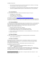
1.6. Other programs
If the user wishes to use the advanced options for the logistics module (please refer to Section
3.6 or 1 for details), it is also required to have:
Java runtime environment (jre). Platform: 1.6. Product: 1.6.0_17 (later program versions
are also possible to use)
Location for the above programs: http://www.java.com/sv/download/
1.7. Samgods GUI installation
Unzip the zipped file Samgods.rar, and select a destination folder. The default folder is C:\,
however, any other folder is working as well. It is recommended to select a folder name without
any blank value. Moreover, an advice is to put the folder rather close to the root (e.g.,
E:\Samgods\Workfolder\Destination-of-folder) since the path to Emme may contain maximum 64
digits.
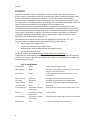
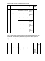
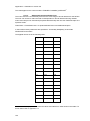
The folder structure for the GUI is displayed in Table 1.
C:\Samgods\
Samgods.cat
Catalog file
01_Programs
Folder
02_Applications
Folder
03_GIS_Data
Folder
04_Media
Folder
05_Input_Data
Folder
06_Reports
Folder
07_Python
Folder
Scenario_Tree
Folder
User_programs
Folder
Table 1 Folder structure.
The scenario folder for a specific scenario is located in the Scenario_Tree folder.
For the complete list of folders and files, see the technical documentation of the Samgods GUI.
To properly install all the programs connected to the model (GIS tools, user programs), do the
following:
1) Open the catalog file (Samgods.cat) in Cube Base (double click on the catalog file or
double click on the Cube icon on the desktop -> welcome screen -> open an existing
catalog -> browse to Samgods.cat)
2) To update the paths for the application, double click on each application (in total 10
applications) under “Applications” window, and click “Yes” to the following question (10
times):
“The base path of this Application has been moved from {Old folder} to {Selected folder}.
Do you wish to update the path for all Application (.APP, .PRJ) and Control (.CTL) files in
the Application structure? (Note the same subdirectory structure as in the original
Applications will be assumed)”
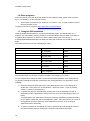
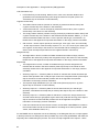
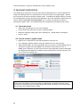
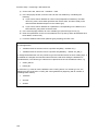
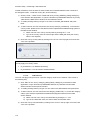
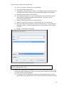
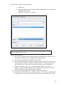
3) To set the properties of the catalog file, start by right-clicking on the Samgods.cat file in
the Cube interface (see the catalog name under the main toolbar) and select
12
Installation Instructions
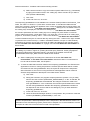
“Properties”. On the Catalog Properties window, select the “Model User” tab, and set the
Model User as “Model Developer”. Then, select the “Data Panel” tab, and set the values
as in Figure 1
Figure 1 Setting of properties of the catalog file.
4) Click “OK” to continue
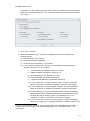
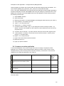
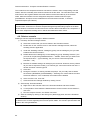
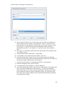
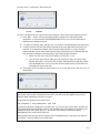
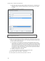
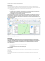
5) Modify the catalog keys (i.e., parameter settings) below from the interface in the
following manner:
a) Select Scenario_Tree scenario
b) Select the Installation application
c) Double-click on the Scenario_Tree scenario
d) For the following catalog keys, change to its corresponding installed version if
3
needed (see Figure 2 for an example):
i)
“Cube Software” (pre-defined: version 6.1.0 Sp1)*
ii)
“EMME Software” (pre-defined: version 3.3.4)
iii) “ArcGIS Software” ( pre-defined: 10.1 Sp1)*
iv) “Python Software” (pre-defined: version 27)
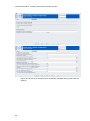
v) “Logistics Model Software” (pre-defined: 20140317)
vi) For the catalog key “Location of Cube Program” change if needed the
folder where Cube is installed (pre-defined: C:\Program Files (x86)\)*
vii) For the catalog key “Location of EMME Program” change if needed the
folder where Emme is installed (pre-defined: C:\Program Files (x86)\)
viii) For the catalog key “Location of ArcGIS Program” change if needed the
folder where ArcGIS is installed (pre-defined: C:\\Program Files (x86)\)*.
Because this path is used by Python, it is important to use “/” or “\\”
instead of “\” in this key, see Figure 2 below for an example
ix) For the catalog key “Location of Python program” change if needed the
folder where Python 26 is installed (pre-defined: C:\Python27\ArcGIS10.1)
3
If you are using Swedish Windows 7/8, the system name of the standard Program folder is
Program Files. So in the keys in the Installation application, use “C:\Program Files\...”, not
“C:\Program\...”.
13
Installation Instructions
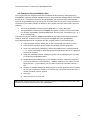
x) For the catalog key “Scenario name for the BASE scenario” point to the
scenario that should be used as base scenario (pre-defined: Base2006)
Figure 2 Example of catalog key values for the Installation application.
e) Run the Installation application by clicking “Run” in the scenario interface, or by
selecting Application -> Run Application -> OK on the main toolbar (If “OK” is clicked
instead of “Run”, the application will not run – the changes in the settings will only be
saved.)
Now the GUI is installed.
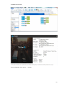
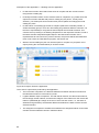
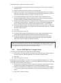
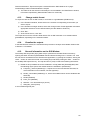
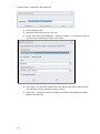
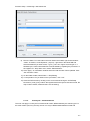
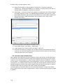
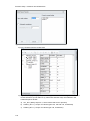
* To properly set the values for the catalog keys indicated with *, see the information under the
Menu Bar Help -> About (see Figure 3 and Figure 4 below for an example).
14
Installation Instructions
Figure 3 How to access the “About ...” information.
Figure 4 Example of the “About ... “ window.
15
Cube Interface components
2. Cube Interface components
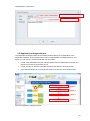
This chapter outlines the main components of the Cube Interface and explains their functions.
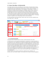
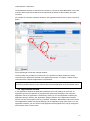
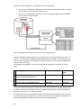
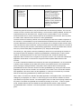
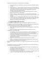
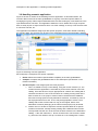
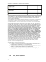
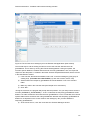
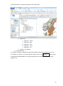
The Cube Interface has five different windows as shown in Figure 5. When opening the model,
two different user types can be selected – model developer or model applier. The model
developer role is mainly used when setting up or installing the system, while the model applier
role typically is used when running the model and for scenario handling. The set of active
windows depends on the user role, and this manual is relevant to both types of model users.
The large area to the right is a workspace where manager windows and messages are shown,
e.g., when the user wants to manage a scenario, the Scenario manager window is shown here.
There are also Application manager windows and Data section manager windows. The manager
windows are opened from the corresponding window on the left hand side.
For more information on the Cube interface, please refer to the Cube Help, accessed from the
main toolbar: Help -> Cube Help.
Scenarios
window
Data
Section
window
Application manager window
Applications
window
Keys
window
Figure 5 Cube Interface and the five windows.
2.1. Scenarios window
The purpose of the Scenarios window is to list the scenarios that exist in the model.
A scenario refers to a set of specific input files/values. An application is a group of programs. In
the Samgods GUI a set of applications are defined with different types of functionalities. Different
scenarios can be set up in the GUI by using the set of available applications. A scenario can be
opened and managed using different applications by double-clicking on the scenario name in the
Scenarios window (in model applier mode). For example, the input data and parameters to the
scenario can be displayed or edited. When the scenario is open in the Scenario manager
window, it is possible to select the application you want to use by the scroll down menu. Another
way to open the application you want to use is to select the application in the Applications
window and then double-click on the scenario in the Scenarios window. The application is then
run by clicking “Run”.
The tree structure of the scenarios included in the Samgods GUI is visualized in the
Scenario_Tree in the Scenarios window. The Scenario_Tree is used for scenario management.
16
Cube Interface components
The default base scenario is included in the Scenario_Tree and is called Base2006. In the base
scenario all the input data is defined and it represents the parent for future sibling and child
scenarios.
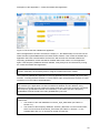
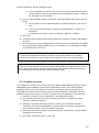
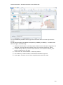
An example of a Scenario manager window for the application Edit the data is given in Figure 6
below.
Key
s
Figure 6 Example of Scenario manager window.
The keys which are possible to set values for in the Scenario manager window are strictly
connected to the application selected in the Applications window. In Chapter 3, tables of keys
connected to the respective applications are presented.
Tip. Open an application (in model applier mode) to set the parameters for a particular
scenario by double-clicking on the scenario and select the application in the scroll down menu.
2.2. Applications window
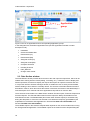
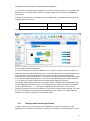
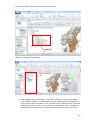
In the Applications window all applications defined in the model catalog can be found. An
application group is the collection of programs and sub-groups belonging to the respective
application. When an application is selected (by clicking on it in the Applications window) the
application group is shown in the Application manager window. In the Application manager
window you can see Program boxes (e.g. MATRIX, HIGHWAY, NETWORK, and PILOT) and/or
other applications (called sub-groups) belonging to the application group (see Figure 7). In the
Applications window, you can see the main application at the highest level, and go through the
tree structure down to lower levels.
17
Cube Interface components
Application
group
Figure 7 View of an application and its corresponding application groups.
In the Samgods GUI, the defined applications are (see the Applications window in model
developer mode):
Installation
Create the editable files
Edit the data (VY)
Edit the data (EM)
Samgods model (VY)
Samgods model (EM)
Compare Scenarios
Handling Scenario
PWC_Matrices
Change matrix format
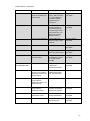
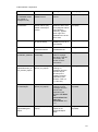
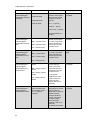
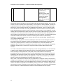
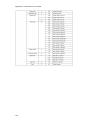
2.3. Data Section window
The Data Section window provides direct access to the main input and output files, which can be
utilized when working with the model (editing, controlling, etc.). It allows the user to display and
edit the input data, as well as to display the outputs and reports for specific scenarios and runs.
In conjunction with the Scenario manager window, it enables the user to easily access all data,
without needing to know where it is actually stored. The structure of the Data Section window is
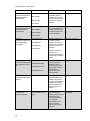
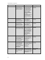
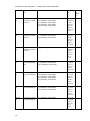
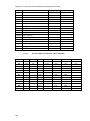
described in Table 2, which also shows the location of the files, the names of the tables/maps, a
short description of its contents and which application that produces or uses the files.
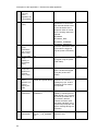
There are three main folders in the Data Section window: Scenario Inputs, Scenario Outputs and
Scenario Reports. The General tables under Scenario Inputs are always accessible from the
Data Section window. The Editable data (also found under Scenario Inputs) is accessible only
during the edit phase or if the user has selected not to delete the temporary geodatabase (see
explanation for the Edit the data applications in Section Fel! Hittar inte referenskälla. and
Section Fel! Hittar inte referenskälla.).
The available output in the Scenario Outputs folder depends on the choices made when running
the Samgods Model application. The available outputs in the folder Scenario Outputs\Samgods
18
Cube Interface components
Report are always listed in the log report Scenario Outputs\Samgods Report\Existing Outputs.
There are two other log reports except Existing Outputs: Report for the import phase and Report
for the edit phase, which state any error messages or other messages from the applications
Handling scenario and Edit the data. For more information on the log reports, see Table 2 and
Chapter 6.
Moreover, the Data Section window includes the 11 standard reports, also called summary
reports, which summarize the output from running the Samgods GUI, in Word format. The
summary reports are found in the Scenario Reports folder and are listed last in Table 2. To
browse to different pages in the reports, use the arrows in the main toolbar. It is possible to
export the tables to Excel, by selecting the table in the Word format report, right-clicking and
selecting “Export” and type in a name with an Excel file format ending. Some of the standard
reports are also available as spread sheet reports in the Scenario Outputs folder, where they are
marked with the same report number as in Scenario Reports (see, e.g., Scenario
Outputs\Samgods Report\Logistic Module\OD Covered).
For some of the data files, the variable names that appear in the headings are explained in
tables in the appendix.
Before using and analyzing any output data regarding empty vehicles/vehicle kilometres or the
total number of vehicles (i.e. loaded + empty vehicles), please read the section about empty
vehicles in the appendix.
The GUI allows producing different aggregations in the results. The model could produce the
total number of loaded, empty and tones for all the commodity groups, or just for a specific
commodity or STAN group. The outputs will be saved with different name files ending with a
number of a suffix. Depending on the user choice the possible values could be:
0 (zero): all the commodities are aggregated, so the volumes and tons are totals
A number among 1 and 35: a single commodity has been ran
A subfix STAN1 to STAN12: an aggregation of results based on STAN group definition
To access at the different aggregations, e.g. different files, it is requested to set the value for
catalog key “Select commodities for the Logistics module (…)” in the Samgods Model application
to the commodity or commodity group number you want to view and clicking “Save” (please refer
to Section 3.6 or 1 for more information).
Folder
Name
Scenario Inputs
Description
Used by application
This folder contains
all the inputs for the
scenarios
All
Scenario
Inputs\Model
Operating instructions
VY
Model Operating
Instructions VY
Rtf file with a short
description on how to
run the Samgods GUI
All (except the EMME
applications)
Scenario
Inputs\Model
Operating instructions
EM
Model Operating
Instructions EM
Rtf file with a short
description on how to
run the Samgods GUI
All (except the
Voyager applications)
19
Cube Interface components
Folder
Name
Description
Used by application
Scenario
Inputs\General tables
Link Categories
Lookup table for the
categories in the
network
All
NodeClass
description
Lookup table for the
numbering system (no
longer required for the
VY part)
All
Transfer Type at
terminals
Lookup table for the
transfer type coded in
the
Nodes_Commodities
data
Samgods Model
(VY) /(EM)
List and codes for
modes (only visible in
developer mode)
Alphanumerical codes
for modes
All
Zoning System
Lookup table for the
ID_Region and
ID_Country codes
All
Modes
Lookup table for
codes used for modes
All
V101 SpeedFlow
Curves
Speed flow table with
parameter values for
defining the delay
functions for vehicle
class 101 (light lorry)
Samgods Model
(VY) /(EM)
V102 SpeedFlow
Curves
Same as previous but
for vehicle classes
102-105
Samgods Model
(VY) /(EM)
Ranges for classes
(only visible in
developer mode)
For node classes from
12 to 19 the range of
allowed values for
node numbers
Edit the data
(VY)/(EM)
Default values for the
frequency matrices
(only visible in
developer mode)
Default frequencies
for different vehicle
classes based on the
terminal type
Edit the data
(VY)/(EM)
Main vehicle class for
BuildChain
The main vehicle
class used in the
BuildChain process
by mode no. (i.e.
vehicle category A-U)
and commodity class
(P1-P35).
Samgods Model
(VY) /(EM)
Scenario
Inputs\General
tables\Logistics
module (only visible in
developer mode)
20
Cube Interface components
Folder
Scenario
Inputs\Editable data
Name
Description
Used by application
Vehicle types by
chain and vessel type
(ChainChoi)
List of vehicle types
(VHCL_NR) by mode
no. and vessel type
(see table Vessel
Type below) for
ChainChoi
Samgods Model
(VY) /(EM)
Direct Access
Whether or not direct
access is active by
commodity type (P1P35) and type of firmto-firm flow (0-9, see
table Type of Flow
MATRIX below)
Samgods Model
(VY)/(EM)
Type of Flow MATRIX
Lookup table with
codes for type of flow
matrices
Samgods Model
(VY)/(EM)
List of Chains
List of Chain types
Samgods Model
(VY) /(EM)
Vessel Type
Lookup table with
codes for vessel types
Samgods Model
(VY) /(EM)
Consolidation factors
by chain (new)
Individual
consolidation bounds
for all sub modes
[LB,HB]
Samgods Model
(VY) /(EM)
Input_Data.mxd
General map to
visualize all
georeferenced data
Edit the data
(VY)/(EM)
EMME Network (211
format) (only visible in
developer mode or for
Emme users)
The Emme transport
network with all link
and node attributes
Samgods Model (EM)
EMME Speed table
(only visible in
developer mode or for
Emme users)
Emme speed tables
Samgods Model (EM)
General parameters
(only visible in
developer mode)
Table with the
scenario parameters
catalog key settings
Edit the data
(VY)/(EM)
Logistics model
parameters (new)
Table with logistics
module parameters
Edit the data
(VY)/(EM)
Cargo Table
General values per
commodity type
Edit the data
(VY)/(EM)
21
Cube Interface components
Folder
22
Name
Description
Used by application
Vehicles Parameters
General values for
each vehicle type.
The attribute
“EMPTY_V” (1 or 0)
regards whether the
number of empty
vehicles will be
calculated (1) or not
(0) (see the appendix
and Section 5.4)
Edit the data
(VY)/(EM)
Scenario Network
Network (links and
nodes) for all modes
(GIS map)
Edit the data
(VY)/(EM)
Nodes Commodities
GIS map with all
terminals and
specifications on
allowed transfer types
and commodities per
terminal
Edit the data
(VY)/(EM)
Nodes
GIS map of zones
and terminals with
values for the logistics
module
Edit the data
(VY)/(EM)
Ports Sweden
GIS map of Swedish
ports with the pilot
fees by vehicle type
(sea mode only)
Edit the data
(VY)/(EM)
Frequency network
GIS map with service
frequencies
(transports per week)
per mode/combination
of modes and origindestination
connection. For more
information on the
frequency network,
see the appendix
Edit the data
(VY)/(EM)
Tax by country
Tax by country and
vehicle type
Edit the data
(VY)/(EM)
Tax by Linkclass
Tax by link type and
vehicle type
Edit the data
(VY)/(EM)
Tax by link
Tax for specific links
by vehicle type
Edit the data
(VY)/(EM)
Toll bridges
Tolls for bridges per
vehicle type
Edit the data
(VY)/(EM)
Cube Interface components
Folder
Name
Description
Used by application
Scenario
Inputs\EMME tables
(only visible in
developer mode)
Default values for the
EMME macros
Labels for Emme
macros
Samgods Model (EM)
Scenario
Inputs\Others
Inzone distances –
default values (only
visible in developer
mode)
Default values of
distances within each
zone (diagonal values
in the distance
matrices). Applied
when origin and
destination are in the
same zone
Samgods Model
(VY) /(EM)
EMME (only visible
for Emme users)
Path to the Emme
databank (not a file, it
is a location)
Samgods Model (EM)
Geodatabase file for
exported matrices
Location of the
geodatabase file
Change matrix format
Scenario
Inputs\PWC_Matrices
PWC matrix for
commodity
Displays the PWC
matrix in Voyager
format for a specific
commodity, see
Section 3.10 for
instructions
PWC_Matrices
Scenario
Outputs\Scenario_Im
port_function_Report
Report for the import
phase (Log report)
Report with any
warnings or
messages from the
Scenario import
function (in the
Handling scenario
application) (see
Sections 3.9/4.10/
4.11 and 6.3)
Handling scenario
Scenario Outputs\Edit
the data Report
Report for the edit
phase (Log report)
Report with any
warnings or error
messages from the
Edit the data
application (see
Sections Fel! Hittar
inte
referenskälla./Fel!
Hittar inte
referenskälla. and
6.1)
Edit the data
(VY)/(EM)
Scenario
Outputs\Samgods
Report
Existing Outputs (Log
report)
List of available
outputs in the
Samgods Report
folder
Samgods Model
(VY)/(EM)
23
Cube Interface components
Folder
Name
Description
Used by application
Scenario
Outputs\Samgods
Report\LOS matrices
generation
LOS Road Mode
Samgods Model
(VY)/(EM)
LOS Sea Mode
LOS matrices
between zones (both
terminals and actual
zones) per vehicle
type for:
LOS Air Mode
time – T [hours],
LOS Rail Mode
distance – D [km],
extra costs – X [SEK],
domestic distances –
DD [km]
Scenario
Outputs\Samgods
Report\Logistics
Module\OD Vehicles
MAT
Road – Vehicle Flows
Rail – Vehicle Flows
Sea – Vehicle Flows
Air – Vehicle Flows
Scenario
Outputs\Samgods
Report\Logistics
Module\OD Tonnes
MAT
Road – Goods Flows
Rail – Goods Flows
Sea – Goods Flows
OD matrices of
loaded vehicle flows
by mode. The sheet
name indicates the
vehicle type and the
scenario name
Samgods Model
(VY)/(EM)
OD matrices in tonnes
by mode. The sheet
name indicates the
vehicle type and the
scenario name
Samgods Model(VY)
/(EM)
OD matrices of empty
vehicle flows by
mode. The sheet
name indicates the
vehicle type and the
scenario name.
Samgods Model
(VY) /(EM)
Air – Goods Flows
Scenario
Outputs\Samgods
Report\Logistics
Module\OD Empty
Vehicles MAT
Road – Empty vehicle
Flows
Rail – Empty vehicle
Flows
Sea – Empty vehicle
Flows
Air – Empty vehicle
Flows
Scenario
Outputs\Samgods
Report\Logistics
Module\OD Covered
24
Output by vehicle
class (spread sheet
for summary report
no. 2: Logistics
module)
For important
explanations of the
output in terms of
empty vehicles,
please refer to the
appendix
Summary table with
information by vehicle
type (number of
shipments, number of
loaded vehicles,
transport distance,
tonnes, tonne kms,
average loading
factor, average
distance), split up on
domestic,
international and total
Samgods Model
(VY)/(EM)
Cube Interface components
Folder
Name
Description
Used by application
Output by chain
(spread sheet for
summary report no. 2:
LM chains)
Summary table with
information by chain
type (total numbers of
shipments, transport
distance, tonnes,
tonne kms, logistic
cost, average cost per
tonne km), split up on
domestic,
international and total
Samgods Model
(VY)/(EM)
Loaded Demand
(spread sheet for
summary report no. 2:
LM Demand) (new)
Summary table of the
tonnes transported
and the tonnes in the
PWC-matrices
together with success
Samgods Model
(VY)/(EM)
Report #5 Logistics
costs at zone level
(Spread sheet for
summary report no. 5)
Logistics costs per
zone per commodity
(P01-P35) and
import/export at zone
level
Samgods Model
(VY/(EM)
Report #6 Goods flow
through terminals
(Spread sheet for
summary report no. 6)
Goods flow (tonnes)
through terminals per
commodity (P01-P35)
and divided by import
(DAIMPORN), export
(DAEXPORN) or
regular (REGULARN).
Regular: goods flow
from and to other
terminals.
Import/export: goods
flow with direct
access from/to a zone
Samgods Model
(VY/(EM)
Report #7 Domestic
tonne kms with
container per mode
(road, rail, sea, air)
(Spread sheet for
summary report no. 7)
Transport work (tonne
kms) in Sweden for
containers per
commodity and mode
Samgods Model
(VY/(EM)
Report #8 Domestic
vehicle kms with
container per mode
(road, rail, sea, air)
(Spread sheet for
summary report no. 8)
Traffic work (vehicle
kms) in Sweden for
containers per
commodity and mode
Samgods Model
(VY/(EM)
25
Cube Interface components
Folder
Name
Description
Used by application
Report #10 Tonnes
km per mode,
commodity, domestic,
tdomestic and
international (Spread
sheet for summary
report no. 10)
Transport work (tonne
kms) per commodity,
mode and
domestic/total
domestic/international
Samgods Model
(VY/(EM)
Report #11 Tonnes
per mode, commodity,
domestic, tdomestic
and international
(Spread sheet for
summary report no.
11)
Tonnes per
commodity, mode and
domestic/total
doemastic/internation
al
Samgods Model
(VY/(EM)
Report#12 node and
link costs per vehicle
and product group
(Spread sheet for
summary report no.
12)(new)
Link and node costs
per vehicle class, per
commodity and total
domestic/
international
Samgods Model
(VY/(EM)
Scenario
Outputs\Samgods
Report\Logistics
Module\Other
TFL road mode
(spread sheet for
summary report no. 3)
Distribution of the
time length of trips for
road mode. For each
time length value
(TIME, increasing by
2 hours in each step),
the no. of vehicles
(SUM), the fraction
and the accumulated
fraction are listed. For
a diagram, see the
corresponding
standard report
(report no. 3 under
Scenario Reports)
Samgods Model
(VY/(EM)
Scenario
Outputs\Samgods
Report\Assignment
Road Assigned
Network
GIS map with the
assignment of the
freight flows to the
transport network per
mode, in tonnes,
loaded and empty
vehicles per vehicle
type. For important
information on the
empty vehicles,
please refer to the
appendix
Samgods Model
(VY)/(EM)
Rail Assigned
Network
Sea Assigned
Network
Air Assigned Network
26
Cube Interface components
Folder
Name
Description
Used by application
Scenario
Outputs\Samgods
Report\Reports
Assigned Network
GIS map with the
assignment of the
freight flows to the
transport network with
all modes in the same
network, in tonnes,
loaded and empty
vehicles per vehicle
type. For important
information on the
empty vehicles,
please refer to the
appendix
Samgods Model
(VY)/(EM)
Report #1 VHL and
VHCLKM (Spread
sheet for summary
report no. 1)
Summary table of
number of vehicles
and vehicle kms per
vehicle class and
mode (split up on
total/domestic and
loaded/empty/all
vehicles). For
important information
on the empty
vehicles, please refer
to the appendix
Samgods Model
(VY)/(EM)
Report #4 TONNES
AND TONNESKM
(Spread sheet for
summary report no. 4)
Summary table of
tonnes and tonne kms
(domestic,
international and total)
per vehicle type and
mode
Samgods Model
(VY)/(EM)
Report #9 Vehicle
kms, tonne kms,
empty vehicle kms
and total vehicle kms
per geographic region
per mode (road, rail)
(Spread sheet for
summary report no. 9)
Summary table of
vehicle kms (split up
on loaded, empty and
all vehicles) and
tonne kms per
geographic region
and mode (road and
rail). For important
information on the
empty vehicles,
please refer to the
appendix
Samgods Model
(VY)/(EM)
LOS Road Dif
Absolute cost
differences between
the current scenario
and the base scenario
for the LOS matrices
Compare Scenarios
Scenario
Outputs\Compare\LO
S Calculation
LOS Rail Dif
LOS Sea Dif
LOS Air Dif
27
Cube Interface components
Folder
Name
Description
Used by application
Scenario
Outputs\Compare\Log
istics Module\OD
vehicles MAT
Road OD Dif
Absolute differences
in loaded vehicles
between the current
scenario and the base
scenario for the OD
matrices
Compare Scenarios
Absolute differences
in tonnes between the
current scenario and
the base scenario for
the OD matrices
Compare Scenarios
Absolute differences
in empty vehicles
between the current
scenario and the base
scenario for the OD
matrices.
Compare Scenarios
Rail OD Dif
Sea OD Dif
Air OD Dif
Scenario
Outputs\Compare\Log
istics Module\OD
Tonnes MAT
Road TON Dif
Rail TON Dif
Sea TON Dif
Air TON Dif
Scenario
Outputs\Compare\Log
istics Module\OD
empty MAT
Road EMP Dif
Rail EMP Dif
Sea EMP Dif
Air EMP Dif
Please refer to the
appendix for
important information
on the empty vehicles
output
Scenario
Outputs\Compare\Log
istics Module\Tot Gen
Att
TRIPEND Road Dif
TRIPEND Rail Dif
TRIPEND Sea Dif
TRIPEND Air Dif
Total generation (sum
of each row) and
attraction (sum of
each column) for the
vehicle OD matrices
and absolute
differences to the
base scenario
Compare Scenarios
Scenario
Outputs\Compare\Ass
ignment
Compared Load Net
GIS map with
absolute differences
between the current
scenario and the base
scenario of loaded
vehicles flows for all
vehicle types and
modes
Compare Scenarios
Scenario Reports
(contains the
summary reports)
Report_1_Tot VHC
and VHCKM by VHC
Type
Number of vehicles
and vehicle kms:
loaded, empty and all,
per vehicle type.
Domestic and total.
For important
information on the
empty vehicles,
please refer to the
appendix
Samgods Model
(VY)/(EM)
28
Cube Interface components
Folder
Name
Description
Used by application
Report_2_Logistics
Module
Summary table of no.
of shipments, no. of
loaded vehicles,
transport distance,
tonnes, tonne kms,
average load factor
and average distance
by vehicle type, split
up on domestic, total
and international
Samgods Model
(VY)/(EM)
Report_2_LM_CHAIN
S
Summary table of no.
of shipments, costs,
kms, tonnes, tonne
kms and average
logistic costs per
tonne km, by
transport chain type
Samgods Model
(VY)/(EM)
Report_2_LM_DEMA
ND (new)
Summary table of the
tonnes transported
and the tonnes in the
PWC-matrices
together with success
rate
Samgods Model
(VY)/(EM)
Report_3_TFL_Distrib
ution
Trip time length
distribution for road
mode. Number of
vehicles making trips
lasting 2, 4, 6, ...
hours
Samgods Model
(VY)/(EM)
Report_4_Tot
TONNES and
TONKM by VHC type
Summary table of
tonnes and tonne kms
(split up on domestic,
international and total)
for each vehicle type
Samgods Model
(VY)/(EM)
Report_5_Total
logistic cost at zonelevel
Total logistics costs
per commodity type
(P01-P35) split by
import and export at
geographical zone
level
Samgods Model
(VY)/(EM)
29
Cube Interface components
Folder
Name
Description
Used by application
Report_6_Goods flow
through terminals
(number of tonnes in
and out per year)
No. of tonnes through
terminals (described
as zones) per P01P35 and whether the
goods flow is import,
export or regular.
Regular refers to
goods flows between
terminals.
Import/export refers to
goods flows with
direct access from/to
a zone
Samgods Model
(VY)/(EM)
Report_7_Domestic
tonne kms with
container per mode
(road, rail, sea, air)
Domestic tonne kms
with container per
mode, split by
commodity and total
Samgods Model
(VY)/(EM)
Report_8_Domestic
vehicle kms with
container per mode
(road, rail, sea, air)
Domestic vehicle kms
with container per
mode, split by
commodity and total
Samgods Model
(VY)/(EM)
Report_9_Vehicle
kms and Tonnes kms
per geographic region
Vehicle kms (for
loaded, empty and all
vehicles) and tonne
kms per geographical
region (road and rail
mode). For important
information on the
empty vehicles,
please refer to the
appendix
Samgods Model
(VY)/(EM)
Report_10_Transport
work (tonne kms) per
mode, total and split
per commodity,
domestic, tdomestic
and international
Transport work (tonne
kms) per mode and
commodity, as well as
domestic, total
domestic or
international
Samgods Model
(VY)/(EM)
Report_11_
Transported goods
volume per mode,
total and split per
commodity, domestic,
tdomestic and
international
Transported goods (in
tonnes) per mode and
commodity, as well as
domestic, total
domestic or
international
Samgods Model
(VY)/(EM)
Report_12_node and
link costs per vehicle
and product group
(new)
Node and link costs
per vehicle type and
product group, divided
in total domestic and
international
Samgods Model
(VY)/(EM)
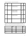
Table 2 List of inputs and outputs accessible from the Data Section window.
30
Cube Interface components
2.4. Keys window
When we look at the GUI, applications present in there represent calculations and formulas we
will apply to the input data. The key window allows to access to all the input data that could vary
in different executions applying the same calculations defined in the application. So a e general
definition of a key is a varying input to an application. For instance using a key it is possible to
specify different values for a parameter, different networks for the LOS calculation and
assignment, different control parameters for the Logistics Module or more.
In general terms the keys may serve different purposes in summary:
To manage input data
To give general settings for the model
To enable different ways to run the model
A key can for example be:
The name of an input data file
A directory
A check box with true or false value
A check list to choose a specific value
A constant
A radio button
Different kinds of keys appear in applications and other places where it is possible to select the
settings.
In Chapter 3, the available catalog keys for each specific application are listed. Catalog keys are
defined as keys for setting up parameters in the applications. The Keys window is available in
developer mode and it is also possible to display from Main toolbar -> Scenario -> View -> Show
Keys.
The following keys in the Cube interface are called system keys:
{CATALOG_DIR} is the directory where the .cat file is located
{SCENARIO_DIR} is the directory where the scenario folder is located
{SCENARIO_CODE}, {SCENARIO_SHORTNAME) are defined in the Scenario
Properties, see Figure 9 below
{SCENARIO_FULLNAME} =
{SCENARIO_SHORTNAME_PARENT}.{SCENARIO_SHORTNAME}, where
{SCENARIO_SHORTNAME_PARENT} is the base scenario to the current scenario
These keys are important components in each scenario. Please refer to the online Cube Voyager
help available from the menu bar for further information (see for instance Scenario Manager >
Working with applications and catalogs > Cube Voyager and TP+ scripts). “Scenario properties”
is accessed by right-clicking on the topical scenario in the Scenarios window and select
“Properties” (see Figure 8).
Each time a scenario is created all catalog keys should be given a value. Some of the keys have
a default value. If the default value is changed by the user, it will become specific for that
scenario. When a scenario is created as the child to another scenario, it will inherit all the catalog
key settings from the parent.
In the Keys window information on the origin of the keys can be found. The keys for a specific
scenario and application can be viewed by selecting the scenario in the Scenarios window by
31
Cube Interface components
clicking on it, and selecting the application in the Applications window in the same way. The keys
marked in black in the Keys window are undefined. The keys are shown in bold font if they have
been explicitly defined by the user and in italics if they have been inherited from the parent
scenario. If the value is in grey font, it is a default value that has not been changed by the user,
neither for the current scenario, nor for its parent.
More information about the keys and the scenarios can be found in the Cube Help, accessed
from the main toolbar (Help -> Cube Help -> Cube Base -> Scenario Manager ->
Keys/Scenarios).
Figure 8 How to open the “Scenario Properties” window.
32
Cube Interface components
{SCENARIO_SHORTNAME}
{SCENARIO_CODE}
Figure 9 Set {SCENARIO_SHORTNAME} and {SCENARIO_CODE} in “Scenario Properties”.
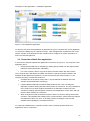
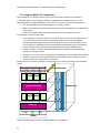
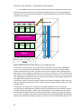
2.5. Application manager window
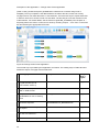
The Application manager window is accessed by double-clicking on an application in the
Applications window, and it provides a flow chart of a transportation modelling process, see
Figure 10. The view is in a hierarchical flow style that offers:
a view of the individual processes, the flow of data from one application to another, the
sequence in which the processes are run
a clear structure of what the input data and the output data are in each process
a convenient interface for running specific parts of the process or the whole model
Execution order
STEP 1
STEP 2
STEP 3
STEP 4
Figure 10 Application manager window.
33
Cube Interface components
2.6. Task Monitor program and the help function
The Task Monitor program is started automatically from the Application manager when the user
runs either a single program or an application. The main purpose of the Task Monitor is to report
the progress of the program/application execution, and to allow control of the run by pausing or
abandoning it. When a run finishes successfully, a message box will indicate that the run is
finished without any problem. If a failure occurred, a dialog box, showing the return code and
error information, will appear.
The return code from the process gives the information on how the run completed. The codes
are shown below.
Return codes:
Return code = 0 – the run completed successfully
Return code = 1 – along the process, a few warning messages were printed but the run was
completed successfully
Return code = 2 – the run ended with a fatal error
Return code = 3 – the process was aborted by the user
There are facilities that allow showing:
The report for the whole run
The report for the step that failed, if the run ended with a fatal error
For more details on the Task Monitor, see reference guide RG_CubeBase.pdf under
Citilabs\Cube folder, Chapter 16.
When the user needs help about the Cube Interface, the help function can be consulted. It is
found on the Menu Bar Help -> Cube Help.
34
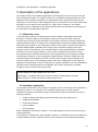
Description of the applications - Installation application
3. Description of the applications
This chapter introduces the different applications in the Samgods GUI, how they are used and
how the settings are made. The chapter is written as a catalog with detailed descriptions of the
applications and should be consulted for the specifications of the applications rather than for
instructions on how to use the entire Samgods model. For instructions on how to get started with
Samgods, how to create and use scenarios etc., please refer to Chapter 4. The chapter
commences with an explanation of the different Model User roles, followed by the description of
the applications in the Samgods model GUI.
3.1. Model User roles
In the Samgods model GUI, two Model User roles are available model applier and model
developer. In general, applier mode should be used by the normal user when setting up
scenarios and running the model. Developer mode should in general be used when advanced
system settings are made, for instance when administrating the system by making installations
and setting up the system. In the catalogue key tables in this chapter, the model user rights are
indicated. Model applier is indicated when the key can be accessed in applier mode (even
though it could be accessed also in the model developer mode). Model developer is indicated
when the key concerns system settings, or when only the developer has access to the key.
As mentioned earlier, the Model User roles are set by right-clicking on the Samgods.cat label
and selecting “Properties”. On the Catalogue Properties window, select the “Model User” tab,
where the settings for the Model User roles are made. More details for when the Model User
roles are used are given in the catalog key tables. Most of the catalog keys for the respective
applications are described however, not all keys are explicitly explained. Two of the applications
(Edit the data and Samgods Model) are available in two versions, depending on whether
Voyager or Emme is used as the supply model.
General guidelines for which Model User role to use:
Model applier – should be used by the normal user when running different scenarios
Model developer – should be used when setting system keys.
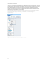
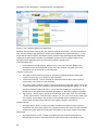
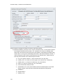
3.2. Installation application
The Installation application is only enabled in developer mode. A screenshot of the application is
displayed in Figure 11. The purpose of the Installation application is to set the general
information to properly run different programs involved in the model. In particular we have the
following programs:
Logistics module (executable programs buildchain.exe and chainchoi.exe)
Citilabs Cube Software
ArcGIS Esri Software
Python software
Emme software
See the installation instructions in Section 1.7 for further details on how to access the keys and
set the right values.
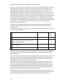
The first group of catalog keys, called “Software versions”, is introduced to avoid inconsistency of
version problems over time. Different versions of the programs can be implemented (typically
35
Description of the applications - Installation application
when a software is updated to a newer version), and it is important to know which software
versions that were used for a particular scenario study to enable proper analysis and consistency
of the outcome. The keys are displayed in Table 3.
Catalog key name
Example of value
Cube Software
6.1.0 Sp1
EMME Software
3.3.4
ArcGIS Software
10.1 Sp1
Python software
27
Samgods Model software
(20140317)
Table 3 “Software versions”.
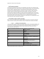
The second group of catalog keys, “Installation parameters”, handles the possible problem of
having different installation folders on different PC’s by setting the path of the programs. Since
the path for the ArcGIS program is used by Python, the “\” signs must be replaced by “/” or “\\” in
this key, see Table 4 for an example.
Catalog key name
Example of value
Location of Cube Program
C:\Program Files\
Location of EMME Program
C:\Program Files\
Location of ArcGIS Program
C:/Program Files/
Location of Python Program
C:\Python27\ArcGIS10.1
Table 4 “Installation parameters”.
The last key in the second group, see Table 5 below, defines the base scenario that is used in
the current model. The base scenario is used as a reference when storing the data for other
scenarios. Only the differences between the base scenario and other scenarios are stored in the
database. The value of this key is related to the Handling scenario application please refer to
Section 3.9 for more information.
Catalog key name
Example of value
Scenario name for the BASE scenario
Base2006
Table 5 Base scenario definition.
36
Description of the applications - Installation application
Figure 11 The Installation application.
To open the overview of the application as illustrated in Figure 11 double-click on the application.
To access the catalog keys of a specific scenario, mark the application, and double-click on the
specific scenario in the Scenario window. Please refer to Chapter 3 for further instructions on
how to use the Samgods GUI.
3.3. Create the editable files application
A view of the Create the editable files application can be seen in Figure 13. The purposes of this
application are to:
Create the essential files for visualizing or editing the input data from the graphical user
interfaces (Cube GIS window, DBI editor)
For a new scenario, allow to copy all the parent scenario data to the new scenario
The concept of this is that all the input data connected to a specific scenario is stored in the
database as the differences between the current scenario and the base scenario (i.e., the
reference scenario). The benefits of this are:
A smaller amount of data is stored, that is, only the differences between the base
scenario and the alternative scenario(s)
It makes different alternative scenarios independent of each other, by letting the
alternative scenarios having only the base scenario as a reference. The only redundancy
of the system occurs when children are added to an alternative scenario since all
scenarios (including child and parent scenarios) are independent of each other and only
have the base scenario as a reference
When changes are made to the base scenario, there is no need to change all the other
scenarios. This facilitates the handling of the overall scenarios. Furthermore the changes
and edits will be done only once, in the base scenario, avoiding the risk of made
mistakes when updating the correlated scenarios
To create the editable files for a specific scenario and the scenario specific tables, two
applications work in conjunction:
37
Description of the applications - Create the editable files application
the Create the editable files application, that merges the base scenario with the scenario
specific tables to view and edit a scenario, and
the Edit the data application, that stores the scenario-specific tables into the database
after any edits have been made.
Figure 12 Database structure and scenario data of the Samgods GUI.
The main database is always present in the model, in the 05_Input_data folder (see Table 1 in
Section 1.7). The temporary database (Scenario_data.mdb) is created in the scenario folder in
each run of this application and is deleted on request by the user. The temporary database can
also be viewed in the GUI.
The catalog keys available in the Create the editable files application are shown in Table 6
below.
Catalog key name
Example of value
Model User’s
rights
1
Which scenario do you want to copy as new
scenario? (Default is Base2006)
Base2006
Applier
2
Location of Python program
C:\Python27\ArcGIS10.1
Developer
3
Scenario name for the BASE scenario
Base2006
Developer
Table 6 Create the editable files catalog keys.
The first key is relevant during the creation of a new scenario. When the scenario already exists,
no action is needed. The last two keys are for installation purposes only. After the Installation
application has been run, no action is required.
To create a new scenario, the application copies the scenario-specific tables from the scenario
(as indicated in the first catalog key in Table 6) and stores them in the temporary database. The
Edit the data application will then store them back to the main database.
38
Description of the applications - Create the editable files application
Figure 13 The Create the editable files application.
When the application has been executed, the output (i.e., the editable files) can be found in the
folder Scenario Inputs\Editable data in the Data Section window. If the Create the editable files
application has been executed before and the user after that has not selected to delete the
temporary geodatabase, all the data will be available without the need to run the application
again. If the temporary database has been deleted, it may always be reconstructed by running
the Create the editable files application.
Please note: This application has to be run at least once for each scenario, including the base
scenario. Otherwise, the necessary files for using the scenario will not be created.
The Create the editable files application is the only application that is necessary to run for each
scenario - including the base scenario. For all scenarios other except the base scenario it is also
necessary to run the Edit the data application.
Tip: The date and time of the last modification in of the temporary and the main geodatabase
are checked by the application to avoid inconsistencies between the two datasets. If any
differences are found, the user is asked to choose whether the execution should be completed
(the temporary geodatabase will then be overwritten) or cancelled, so that the temporary
geodatabase could be saved to the main geodatabase by the user.
Please note:
The location of the main database is in the 05_Input_data folder (see Table 1 in
Section 1.7).
The location of the temporary database, Scenario_data.mdb, is in the scenario folder,
which can be found in the Scenario_Tree folder (see Table 1 in Section 1.7). It is
available after each run. It can also be viewed from the GUI.
39
Description of the applications - Create the editable files application
3.4. Edit the data (VY) application
The Edit the data (VY) application should be used if changes to the input data are made in
Voyager. The Voyager applications are only displayed if the settings in the Catalog Properties
indicate that the user is a Voyager user (please refer to Section 4.2). If you are an Emme user,
please refer to Section Fel! Hittar inte referenskälla..
A view of the application is shown in Figure 14. The purposes of the application are to:
Enable editing of the scenario data by using the Scenario manager window or the Data
Section window. All georeferenced data is visualized using the GIS Cube window and
the other data is displayed in a database window. See the reference guide for Cube
Base (RG_CubeBase.pdf under Citilabs\Cube folder) for further information on these
tools
Store the modified data (the scenario-specific tables) to the main database after editing
The catalog keys are ordered in two steps. The first ones are shown in Table 7 below
1
Catalog key
name
Example of value and
explanation of values
Description
Model
User’s
rights
Do you want to
lock the scenario
from further
editing?
Yes
This key is
introduced due to
data security
reasons, where the
user can choose to
lock the scenario
from further editing.
Applier
Further explanation
is given below
2
General
parameters [Table]
C:\Samgods\Scenario_Tree\
Base2006\Scenario_Data.md
b\General_Base2006
This is the scenario
data for the scenario,
generated by the
system
Developer
3
Attribute name for
extra cost on
specific link [SEK]
EC_V
Please refer to
Section 5.1 for
further explanation
Applier
4
Attribute name for
extra cost on
specific link
[SEK/km]
EC_KM_V
Please refer to
Section 5.1 for
further explanation
Applier
5
Daily factor for all
modes (except for
Rail Mode) [days
per year]
365
This key represents
a value used to
convert the annual
flows into hourly
flows and is
expected to be
changed rarely
Developer
40
Description of the applications - Create the editable files application
6
Daily factor for Rail
Mode [days per
year]
250
This key represents
a value used to
convert the annual
flows into hourly
flows and is
expected to be
changed rarely
Developer
7
Peak Hour Factor
0.12
This key represents
a value used to
convert the annual
flows into hourly
flows and is
expected to be
changed rarely
Developer
8
General
parameters for
Logistic Module
[Table] (new)
C:\SamGods\Scenario_Tree\
Base2006\Scenario_Data.md
b\LogMod_Base2006
This is the Logistic
Module data for the
scenario, generated
by the system
Developer
9
Interest rate used
in cost calculation
[%/year] (new)
0.1
Interest rate used in
cost calculations
[%/year]
Applier
10
Stuffing cost [SEK
per tonne] (new)
18
Stuffing cost [SEK
per tonne]
Applier
11
Number of
transport chain
solutions for the
Logistics module
1: the optimal solution
Please refer to Table
5.2 in “Program
documentation for
the logistics model
for Sweden” (see
References). The
output is found in the
Data Section
window, in Scenario
Inputs/Editable data/
General parameters
table, in the field
DATA. In the current
implementation only
the optimal solution
is implemented
Applier
Please refer to Table
5.2 in the “Program
documentation for
the logistics model
for Sweden” (see
References). The
output files are found
in the scenario folder
(see Table 1), in
LogMod\ChainChoi\
OUTPUT and could
be consulted by the
advanced user
Applier
2: the second best solution
…
5: the fifth best solution
12
Output variables
for the optimal
transport solution
[e.g.1,2,3, max is
8]
1: direct access
2: (un)loading costs
3: wait time costs
4: main utilization rate
5: number of vehicles
6: detailed information (total
cost, total distance, total
times, commodity, etc.) per
chain type
41
Description of the applications - Create the editable files application
7: detailed information
(transport cost share, total
distance, total times, mode,
etc.) per OD-leg
8: Statistics of the avail
function
Max is 8.
13
Initial consolidation
factor in
BuildChain (1
iteration)
0.75
14
ALL_LORRY_TYP
E_CONSOL (new)
Yes
15
INDIVIDUAL_OD_
LEG_OPTIMIZE
(new)
Yes
16
MINIMUM_ANNU
AL_TONNE_DEM
AND_4_FREQ_O
PTIMIZE [tonnes]
(new)
10
42
This key concerns
which consolidation
factor (for all modes)
that should be used
in BuildChain. Please
refer to the Method
Report (see the
References, Chapter
8)
This key will enable
the consolidation of
all lorries if the value
is Yes. With No the
implementation will
be the same as
previous Logistic
module version
If true then each
chain is evaluated
one leg at a time,
and the lowest cost
vehicle is chosen.
The exception is legs
rolling on and off a
RoRo vessel, where
the previous,
recursive
optimization method
is used for the three
legs rolling on – roro
– rolling off.
If (Annual Demand /
Nr Relations) <
MINIMUM_ANNUAL
_TONNE_DEMAND_
4_FREQ_OPTIMIZE
ChainChoi will exit
20 step frequency
optimization loop
Applier
Applier
Applier
Applier
Description of the applications - Create the editable files application
after the first
iteration, where
frequency
corresponds to EOQ.
17
Low bound for
consolidation
factor [Tonnes]
(new) (applied to
all commodities)
0.05
18
Upper bound for
consolidation
factor [Tonnes]
(new) (applied to
all commodities)
0.95
19
TONNES (new)
DYNAMIC_MAX
Lower bound bounds
for the consolidation
factors ranking
output
Upper bound bounds
for the consolidation
factors ranking
output
Parameter to control
how the demand
shall be used in the
calculation of the
shipment sizes on
annual flow.
Following values are
allowed:
Applier
Applier
Applier
DYNAMIC,
DYNAMIC_MAX
DYNAMIC_AVERAG
E,
DYNAMIC_GEOME
AN
20
Do you want to log
parameters from
control files? (new)
Yes
21
Do you want to log
reading of input
data? (new)
Yes
22
Do you want to log
cost values from
vehicles files?
(new)
Yes
23
Do you want to
delete the
temporary
geodatabase?
(Tick=yes)
Tick =yes
If true the
parameters from
control file are
logged in log file
(under LOG folder).
If true the input data
phase is logged in
log file (under LOG
folder).
If true the cost values
read from LOS files
are logged in log file
(under LOG folder).
This key gives the
user the possibility to
save hard disk space
by deleting the
temporary
geodatabase
Applier
Applier
Applier
Applier
43
Description of the applications - Create the editable files application
(Scenario_Data.mdb)
. However, by
keeping the
temporary files, there
is no need to run the
Create the editable
files application
again (for the current
scenario)
Table 7 Scenario parameters and handling keys.
The first key (lock the scenario or not) is introduced due to data security reasons. The user can
choose to lock the scenario from further editing. A new scenario is always editable, because it is
expected that the user needs to change some scenario tables. To lock a scenario means that
after the run, all the scenario data can be visualized in the interface, but if any edits are made,
these edits will not be saved in the main geodatabase. The base scenario is locked by default,
and it should always be locked to enable comparison of the scenarios. In the database, only the
relative differences between the base scenario and the scenarios (alternatives) are stored, why it
is important not to change the base scenario when new scenarios have been introduced. The
other scenarios could be locked or not, depending on the user’s choices. A prompt window gives
information whether the scenario is locked or not during the execution of the following
applications: Create the editable files, Edit the data (VY), Edit the data (EM), Samgods Model
(VY), Samgods Model (EM).
The last key (no. 23) gives the user the possibility to reduce the run time during the creation of
the temporary files. By deleting the temporary geodatabase, hard disk space could be saved.
However, by keeping the files, run time can be saved since the Create the editable files
application does not have to be run again for the specific scenario. The Create the editable files
application needs about 5-10 minutes to merge all scenario specific tables with the base
scenario.
To avoid inconsistencies between the temporary and the main geodatabase, it is recommended
to always control whether the two data sets have the same date and time of last modification,
before running the Samgods Model. If they differ, there could be edits in the temporary
geodatabase that have not been saved to the main geodatabase (by running the Edit the data
application) and will not be included in the execution of the model. For the Create the editable
files application, this check is done by the application, in order not to overwrite any not saved
edits in the temporary geodatabase by mistake (see Section 3.3).
When “Next” is clicked in the Edit the data (VY) application in the applier mode, a second set of
catalog keys is displayed, see Table 8. These keys give access from the interface to all the input
data for the specific scenario. The model applier does not need to do anything to define the key
values. The tables and geodata can be edited by clicking on the “Edit…” button in applier mode.
All these files are also accessible from the Data Section window, under Scenario Inputs\Editable
data. In Section 2.3 a brief explanation of all files in the Data Section window is given.
44
Description of the applications - Create the editable files application
Catalog key
name
Example of value
Model
User’s
rights
Name of file in
Data Section
window
ArcMap GIS
Project File
C:\Samgods\Scenario_Tree\Base2006\Input_
Data.mxd
Applier
Input_Data.mxd
Commodity
data [Table]
C:\Samgods\Scenario_Tree\Base2006\Scen
ario_Data.mdb\Cargo_Base2006
Applier
Cargo Table
General
parameters of
Vehicle
Classes
[Table]
C:\Samgods\Scenario_Tree\Base2006\Scen
ario_Data.mdb\Vehicles_Parameters_Base2
006
Applier
Vehicles
Parameters
Table with tax
by country
(SEK/km)
[Table]
C:\Samgods\Scenario_Tree\Base2006\Scen
ario_Data.mdb\Tax_Country_Base2006
Applier
Tax by country
Table
Tax by
Category
(SEK) [Table]
C:\Samgods\Scenario_Tree\Base2006\Scen
ario_Data.mdb\Tax_Category_Base2006
Applier
Tax by Linkclass
Tax by Link
(SEK) [Table]
C:\Samgods\Scenario_Tree\Base2006\Scen
ario_Data.mdb\Tax_Link_Base2006
Applier
Tax by link
Toll for
bridges (SEK)
[Table]
C:\Samgods\Scenario_Tree\Base2006\Scen
ario_Data.mdb\Toll_Link_Base2006
Applier
Toll bridges
Network
specific of
scenario
[Geodata]
C:\Samgods\Scenario_Tree\Base2006\Scen
ario_Data.mdb\Network
Applier
Scenario Network
Port terminals
(pilot fees
values)
[Geodata]
C:\Samgods\Scenario_Tree\Base2006\Scen
ario_Data.mdb\Ports_Swe
Applier
Ports Sweden
Zones and
terminals
attributes
[Geodata]
C:\Samgods\Scenario_Tree\Base2006\Scen
ario_Data.mdb\Nodes
Applier
Nodes
Nodes
commodities
(interchanges
allow)
[Geodata]
C:\Samgods\Scenario_Tree\Base2006\Scen
ario_Data.mdb\Nodes_commodities
Applier
Nodes
commodities
Frequency
data
[Geodata]
C:\Samgods\Scenario_Tree\Base2006\Scen
ario_Data.mdb\Frequency_network
Applier
Frequency
network
Table 8 Editable data.
45
Description of the applications - Create the editable files application
The last two catalog keys are only accessible in model developer mode. They define the base
scenario and the folder for the Python program, see Table 9.
Catalog key name
Example of value
Model User’s rights
Location of Python Program
C:\Python27\ArcGIS10.1
Developer
Scenario name for the BASE scenario
Base2006
Developer
Table 9 Developer keys.
Figure 14 The Edit the data (VY) application.
The output of the Edit the data (VY) application, a log report containing information on the
execution of the application, can be found in the folder Scenario Outputs\Edit the data Report in
the Data Section window. This file contains a list of numbered messages giving information on,
e.g., whether any data is missing in the input data (e.g. a missing port in the ports_swe table).
For a list of messages, see the Chapter 6.
Please Note! This application has to be run at least once for every scenario as Voyager
user– except the base scenario, if no changes are made.
46
Description of the applications - Edit the data (EM) application
3.5. Edit the data (EM) application
This application should be used instead of the Edit the data (VY) application if changes to the
input data are made in Emme. The Emme applications are only displayed if the settings in the
Catalog Properties indicate that the user is an Emme user (please refer to Section 4.2). If you
are a Voyager user, please refer to Section Fel! Hittar inte referenskälla..
A view of the application can be seen in Figure 15. The purposes of the application are:
Enable editing of the scenario data using the Scenario manager window or the Data
Section window. All georeferenced data is visualized using the GIS Cube window and
the other data is displayed in a database window. See the reference guide for Cube
Base (RG_CubeBase.pdf under Citilabs\Cube folder) for further information on these
tools
Import the changes using ascii files, if the changes in the network data have been made
in Emme
Store the modified data (the scenario specific tables) to the main database after editing
The catalog keys are ordered in two steps. The first ones are shown in Table 10 below.
1
Catalog key
name
Example of value
Description
Model
User’s rights
Do you want
to lock the
scenario
from further
editing?
Yes
This key is introduced due
to data security reasons,
where the user can choose
to lock the scenario from
further editing.
Applier
Further explanation is
given below
2
General
parameters
[Table]
C:\Samgods\Scenario_Tre
e\Base2006\Scenario_Dat
a.mdb\General_Base2006
This is the scenario data
for the base scenario
generated by the system
Developer
3
Attribute
name for
extra cost on
specific link
[SEK]
EC_V
Please refer to Section 5.1
for further explanation
Applier
4
Attribute
name for
extra cost on
specific link
[SEK/km]
EC_KM_V
Please refer to Section 5.1
for further explanation.
Applier
5
Daily factor
for all modes
(except for
Rail Mode)
[days per
year]
365
This key represents a
value used to convert the
annual flows into hourly
flows and is expected to be
changed rarely
Developer
47
Description of the applications - Edit the data (EM) application
6
Daily factor
for Rail Mode
[days per
year]
250
This key represents a
value used to convert the
annual flows into hourly
flows and is expected to be
changed rarely
Developer
7
Peak Hour
Factor
0.12
This key represents a
value used to convert the
annual flows into hourly
flows and is expected to be
changed rarely
Developer
8
General
parameters
for Logistics
Module
[Table] (new)
C:\SamGods\Scenario_Tr
ee\Emme2006\Scenario_
Data.mdb\LogMod_Emme
2006
This is the Logistic Module
data for the scenario,
generated by the system
Developer
9
Interest rate
used in cost
calculations
[%/year](new
)
0.1
Interest rate used in cost
calculations [%/year]
Applier
10
Stuffing cost
[SEK per
tonne](new)
18
Stuffing cost [SEK per
tonne]
Applier
11
Number of
transport
chain
solutions for
the Logistic
Module
1: the optimal solution
Please refer to Table 5.2 in
“Program documentation
for the logistics model for
Sweden” (see the
References). The output is
found in the Data Section
window, in the Scenario
Inputs/Editable data/
General parameters table,
in the field DATA. In the
current implementation
only the optimal solution is
implemented
Applier
Output
variables for
the optimal
transport
solution
[e.g.1,2,3,
max is 8]
1: direct access
Please refer to Table 5.2 in
the “Program
documentation for the
logistics model for
Sweden” (see References).
The output files are found
in the scenario folder (see
Table 1), in
LogMod\ChainChoi\
OUTPUT and could be
consulted by the advanced
user
Applier
12
2: the second best solution
…
5: the fifth best solution
2: (un)loading costs
3: wait time costs
4: main utilization rate
5: number of vehicles
6: detailed information
(total cost, total distance,
total times, commodity,
etc.) per chain type
7: detailed information
(transport cost share, total
distance, total times,
48
Description of the applications - Edit the data (EM) application
mode, etc.) per OD-leg
8: Statistics of the avail
function
Max is 8.
13
Initial
consolidation
factor in
BuildChain (1
iteration)
0.75
14
ALL_LORRY
_TYPE_CON
SOL (new)
Yes
15
INDIVIDUAL
_OD_LEG_O
PTIMIZE
(new)
Yes
16
MINIMUM_A
NNUAL_TO
NNE_DEMA
ND_4_FREQ
_OPTIMIZE
[tonnes]
(new)
10
17
Low bound
for
consolidation
factor
[Tonnes]
(new)
(applied to all
commodities)
0.1
18
Upper bound
for
consolidation
0.95
This key concerns which
consolidation factor (for all
modes) that should be
used in BuildChain. Please
refer to the Method Report
(see References)
This key will enable the
consolidation of all lorries if
the value is Yes. With No
the implementation will be
the same as previous
Logistic module version
If true then each chain is
evaluated one leg at a
time, and the lowest cost
vehicle is chosen. The
exception is legs rolling on
and off a RoRo vessel,
where the previous,
recursive optimization
method is used for the
three legs rolling on – roro
– rolling off.
If (Annual Demand / Nr
Relations) <
MINIMUM_ANNUAL_TON
NE_DEMAND_4_FREQ_O
PTIMIZE ChainChoi will
exit 20 step frequency
optimization loop after the
first iteration, where
frequency corresponds to
EOQ.
Lower bound bounds for
the consolidation factors
ranking output
Upper bound bounds for
the consolidation factors
ranking output
Applier
Applier
Applier
Applier
Applier
Applier
49
Description of the applications - Edit the data (EM) application
factor
[Tonnes]
(new)
(applied to all
commodities)
19
TONNES
(new)
DYNAMIC_MAX
Parameter to control how
the demand shall be used
in the calculation of the
shipment sizes on annual
flow. Following values are
allowed:
Applier
DYNAMIC,
DYNAMIC_MAX
DYNAMIC_AVERAGE,
DYNAMIC_GEOMEAN
20
Do you want
to log
parameters
from control
files? (new)
Yes
21
Do you want
to log
reading of
input data?
(new)
Yes
22
Do you want
to log cost
values from
vehicles
files? (new)
Yes
23
Select from
which
interface you
want to
import your
edits:
Emme option 1 (emme
network and speed tables)
If option “GIS window” is
selected, the next two
catalog keys (no. 24 and
25 below) do not need to
be specified
Applier
24
Use emme
network file:
C:\Temp\EMME_NET_Em
me2006.211
The network data can be
edited by importing Emme
data (format: .211). The file
should be specified here. It
is necessary that the
network file exists under
the folder indicated, or the
system will prompt the user
with a message during the
execution
Applier
25
Use emme
speed table:
C:\EMME\NetworkBase20
11\V101_1_02_SPEEDS.
DAT
See key no. 23, except the
format is .DAT
Applier
50
If true the parameters from
control file are logged in
log file (under LOG folder).
If true the input data phase
is logged in log file (under
LOG folder).
If true the cost values read
from LOS files are logged
in log file (under LOG
folder).
Applier
Applier
Applier
Description of the applications - Edit the data (EM) application
26
Do you want
to delete the
temporary
geodatabase
? (Tick=yes)
Tick
This key gives the user the
possibility to save hard disk
space by deleting the
temporary geodatabase
(Scenario_Data.mdb).
However, by keeping the
temporary files, there is no
need to run the Create the
editable files application
again (for the current
scenario)
Applier
Table 10 Scenario parameters and catalog keys.
The first key (lock the scenario or not) is introduced due to data security reasons. The user can
choose to lock the scenario from further editing. A new scenario is always editable, because it is
expected that the user will make some changes to the scenario tables. To lock a scenario
means that after the run, all the scenario data can be visualized in the interface, but if any edits
are made, these edits will not be saved in the main geodatabase.
The base scenario is locked by default, and it should always be locked to enable comparison of
the scenarios. In the database, only the relative differences between the base scenario and the
scenario alternatives are stored, this is why it is important not to change the base scenario when
new scenarios have been introduced. A prompt window gives information whether the scenario is
locked or not during the execution of the following applications: Create the editable files, Edit the
data (VY), Edit the data (EM), Samgods Model (VY), Samgods Model (EM).
The last key (no. 26) gives the user the possibility to reduce the run time during the creation of
the temporary files. By deleting the temporary geodatabase, hard disk space could be saved.
However, by keeping the files, run time can be saved since the Create the editable files
application does not have to be run again for the specific scenario. The Create the editable files
application needs about 5-10 minutes to merge all scenario specific tables with the base
scenario.
To avoid inconsistencies between the temporary and the main geodatabase, it is recommended
to always control whether the two data sets have the same date and time of last modification,
before running the Samgods Model. If they differ, there could be edits in the temporary
geodatabase that have not been saved to the main geodatabase (by running the Edit the data
application) and will not be included in the execution of the model. For the Create the editable
files application, this check is done by the application, in order not to overwrite any not saved
edits in the temporary geodatabase by mistake (see Section 3.3).
When “Next” is clicked in the Edit the data (EM) application in the applier mode, a second set of
catalog keys is displayed, see Table 11. These keys give access from the interface to all the
input data for the specific scenario. The model applier does not need to do anything to define the
key values. The tables and geodata can be edited by clicking on the “Edit…” button in applier
mode. All these files are also accessible from the Data Section window, under Scenario
Inputs\Editable data. In Section 2.3 a brief explanation of all files in the Data Section window is
given.
51
Description of the applications - Edit the data (EM) application
Catalog
key name
Example of value
Model
User’s
rights
Name of file in
Data Section
window
ArcMap
GIS Project
File
C:\Samgods\Scenario_Tree\Base2006\Inpu
t_Data.mxd
Applier
Input_Data.mxd
Commodity
data
[Table]
C:\Samgods\Scenario_Tree\Base2006\Sce
nario_Data.mdb\Cargo_Base2006
Applier
Cargo Table
General
parameters
of Vehicle
Classes
[Table]
C:\Samgods\Scenario_Tree\Base2006\Sce
nario_Data.mdb\Vehicles_Parameters_Bas
e2006
Applier
Vehicles
Parameters
Table with
tax by
country
(SEK/km)
[Table]
C:\Samgods\Scenario_Tree\Base2006\Sce
nario_Data.mdb\Tax_Country_Base2006
Applier
Tax by country
Table
Tax by
Category
(SEK)
[Table]
C:\Samgods\Scenario_Tree\Base2006\Sce
nario_Data.mdb\Tax_Category_Base2006
Applier
Tax by Linkclass
Tax by Link
(SEK)
[Table]
C:\Samgods\Scenario_Tree\Base2006\Sce
nario_Data.mdb\Tax_Link_Base2006
Applier
Tax by link
Toll for
bridges
(SEK)
[Table]
C:\Samgods\Scenario_Tree\Base2006\Sce
nario_Data.mdb\Toll_Link_Base2006
Applier
Toll bridges
Network
specific of
scenario
[Geodata]
C:\Samgods\Scenario_Tree\Base2006\Sce
nario_Data.mdb\Network
Applier
Scenario Network
Port
terminals
(pilot fees
values)
[Geodata]
C:\Samgods\Scenario_Tree\Base2006\Sce
nario_Data.mdb\Ports_Swe
Applier
Ports Sweden
Zones and
terminals
attributes
[Geodata]
C:\Samgods\Scenario_Tree\Base2006\Sce
nario_Data.mdb\Nodes
Applier
Nodes
Nodes
commoditie
s
(interchang
es allow)
C:\Samgods\Scenario_Tree\Base2006\Sce
nario_Data.mdb\Nodes_commodities
Applier
Nodes commodities
52
Description of the applications - Edit the data (EM) application
[Geodata]
Frequency
data
[Geodata]
C:\Samgods\Scenario_Tree\Base2006\Sce
nario_Data.mdb\Frequency_network
Applier
Frequency network
Table 11 Editable data.
The last two keys are only accessible in developer mode. They define the base scenario and the
folder for the Python program, see Table 12 below.
Catalog key name
Example of value
User’s rights
Location of python program
C:\Python27\ArcGIS10.1
Developer
Scenario name for the BASE scenario
Base2006
Developer
Table 12 Developer keys.
Figure 15 The Edit the data (EM) application.
The output of the Edit the data (EM) application, a log report containing information on the
execution of the application, can be found in the folder Scenario Outputs\Edit the data Report in
the Data Section window. This file contains a list of numbered messages giving information on,
e.g., whether any data is missing in the input data (e.g. a missing port in the ports_swe table).
For a list of messages, see the Chapter 6.
Please Note! This application has to be run at least once for every scenario as an Emme
user – except the base scenario, if no changes are made.
53
Description of the applications - Samgods Model (VY) application
3.6. Samgods Model (VY) application
This application is for Voyager users. If you are an Emme user, please refer to Section 1.
A schematic picture of the Samgods Model (VY) application is outlined in Figure 17. The
Samgods Model (VY)/(EM) application is the core of the system, since it has the purpose to:
Run the Samgods model (using Voyager as the supply model)
Make sure that all required input data exists (in the main geodatabase or created along
the process)
Save all the outputs at the right places (depending on the request of the user)
The application has four main steps:
LOS calculation – the step where the Level Of Service matrices are calculated. There is
one LOS matrix for each vehicle type providing transport time, transport distance,
infrastructure fees/charges and the domestic distance for zone-to-zone relations. The
LOS matrices are mandatory input to the Samgods model (Please refer to the Method
Report and/or the VTI report for further explanation, see Section 8 References)
Logistics module – the step where the freight flows of the different commodities are
assigned to transport chains
Assignment – the step where the freight flows are assigned to the infrastructure network
Reports – the step where all standard reports (also called summary reports) from the
Samgods Model (VY) application are produced
Please refer to the reference material, or the Appendix, for further information of the Samgods
model.
COMMODITIES
LOS Calculation
Logistics Module
EXECUTION
Assignment
Reports
Road
Rail
Air
MODE
Sea
Figure 16 Different ways to run the Samgods Model (VY) application.
54
Description of the applications - Samgods Model (VY) application
The Samgods Model (VY) application has different choice dimensions, depending on the results
that the user wants (see Figure 16). To summarize, all the possibilities are:
The model could be run as an uninterrupted process or step-by-step (illustrated in the
figure by the blue arrows to the right)
It is possible to run all the commodities at once or one commodity at the time (illustrated
by the yellow arrow at the top of the figure)
For the steps LOS Calculation and Assignment is it possible to run all the modes or only
a specific mode (illustrated by the green boxes to the left in the figure)
It is possible to select which specific outputs to save from running the Samgods model.
Not all combinations of these choices are allowed. Details are given in the following paragraph.
During the run, the user will be informed with a prompt window whether the selections made are
coherent with each other.
The option to run the model for one mode at a time is allowed only for the steps highlighted in
green, i.e. LOS Calculation and Assignment. This is due to the fact that the Logistics module
needs LOS matrices for all modes. A reason for running only a specific mode could be that the
differences in the input data are related only to one mode. For instance, if no other changes have
been made in the input data, there is no need to rerun the whole scenario in the LOS Calculation
step. Regarding the Assignment step, the user may be interested in examining the assignment of
the freight to the network for only one mode.
The final step, Reports, produces summary reports from running the Samgods model. Since this
step summarizes the three previous steps, a full run of all four modes needs to be done to obtain
complete reports.
It is allowed to run all steps in the Samgods model (VY) application for only one specific
commodity group (as illustrated by the blue arrows). But when doing this the estimation of flows
of empty vehicles gets flawed – please refer to the appendix for more information.
If changes in the input data are detected after the LOS matrices have been created, the program
will prompt the user with a message in the report file in the folder Scenario Outputs\Samgods
report\Existing Outputs in the Data section window. During the execution, the user is provided
with the option to cancel the run (by ticking the answer “Do you want to check data and skip the
process?”). See Chapter 6 for further information on the log reports.
The first key for the Samgods Model (VY) application is the key to define the base scenario. It is
only available in developer mode.
Catalog key name
Example of value
User’s rights
Scenario name for the BASE scenario
Base2006
Developer
Table 13 Developer key.
The next group of catalog keys, “Run Selections”, refers to the execution order, see Table 14.
Catalog key name
Example of
User’s
value
rights
1
Run only one application, or run all steps
All
Applier
2
Select the mode for the LOS Calculation and the
Assignment steps
Road
Applier
55
Description of the applications - Samgods Model (VY) application
3
Select commodities for the Logistics Module (for all
commodities, select 0)
0
Applier
Table 14 “Run Selections” keys.
Possible input values for the first key listed in Table 14 are:
LOS calculation
Logistics module
Assignment
Reports
All – all fours steps
Output is produced from all steps in the Samgods model application. Together with the Microsoft
Office tools (such as Access and Excel) this output can be analyzed in-depth in various ways.
The purpose of the standard reports produced in the Report step is to give the user a quick
overview of the results from running the Samgods model application.
Possible input values for the second key listed in Table 14 are:
All
Road
Rail
Sea
Air
The last key has a more general function. It is used in all the applications where the output data
is filtered by commodity. It is the most important catalog key of these three keys. If the Samgods
model first is run for commodity type 1 (for instance), then for all the commodity types (key set to
zero), then both the results for commodity type 1 and for all the commodities will be saved. In the
scenario folder (under Scenario_Tree, see Table 1), the name of the specific output database is
OutputX_{SCENARIO_SHORTNAME}.mdb, where X is the commodity group. Switching from
one set of output to another in the interface is easily made by changing the value of this catalog
key and clicking “Save”. The possible values for this key are the numbers representing different
commodities or zero, representing all commodities. The possible commodities are the NSTR
commodity types (1-35) and the STAN commodity types (STAN 1-12). See the Appendix or for
instance the Program Documentation (see References) for more information.
The report “Existing Outputs” (in the folder Scenario Outputs\Samgods Report in the Data
Section window) is updated during each run and it gives information on the output and the
commodity class.
The next set of catalog keys, “Other options”, refers to the optional outputs which can be saved
in the scenario folder, see Table 15 below.
Catalog key name
Example of
value
Model User’s
rights
1
Do you want to save the LOS matrices?
Tick
Applier
2
Do you want to save the temporary data into the scenario
folder? (emme files for the LOS matrices, network and
attribute files)
Yes
Applier
3
Do you want to save the output report files from the Logistics
module?
Tick
Applier
56
Description of the applications - Samgods Model (VY) application
4
Do you want to produce buildchainxx.log files?
No
Developer
Table 15 “Other options” keys.
The LOS matrices produced during the cost calculation step are stored in the scenario folder in
Voyager format (i.e. in MAT format).
Key no. 2 allows the user to select whether the temporary data should be saved into the scenario
folder, e.g., Scenario_Tree/Base2006/LogMod. Examples of how the files are saved are: the
LOS matrices as well as the vehicle/empty/tonnes matrices are saved in .314 format and the
input files to the Logistics Module are saved in .txt format.
Regarding key no. 3, the output report files from the Samgods model are saved in the scenario
folder and also converted into geodatabase tables which are possible to handle via the interface
(in Scenario Outputs\Samgods Report\Logistics Module in the Data Section window). The output
files that are created (except the standard output that is always produced by the Samgods
model) depend on user selections. Please refer to the list of available outputs later in this section
to see which output that is affected by this catalog key.
With the fourth key the user selects whether the Buildchain program will produce log files or not.
The log files (*.log) contain any warnings that can occur during the execution. Please refer to the
Program documentation for the logistics model (see References) for more information.
The next group of keys allows the user to set the advanced options for the logistics module
(heading “Logistics module settings – advanced”) and is made up by three catalog keys, see
Table 16 below.
Catalog key name
Example of
value
Model User’s
rights
1
Do you want to run the Logistics module on several
processors?
Yes
Applier
2
How many processors would you like to run
simultaneously?
4
Applier
3
Scaling factor for outputs
Thousands
Applier
Table 16 “Logistics module settings – advanced” keys.
If the computer has more than one CPU available, it is possible to split up the processes
between the CPU:s to speed up the run time of the model, using the catalog keys above. The
third key enables the user to define the scale of the output that will be presented in the reports. If
the value is thousands, the output value (for instance 2.000.000 vehicle kilometres) will be
presented as the value divided by thousand (i.e., 2.000 vehicle kilometres in the example).
57
Description of the applications - Samgods Model (VY) application
Figure 17 The Samgods Model (VY) application.
Based on the selections made by the user, different outputs are created – one set of outputs for
each specific setting of the catalog key “Select commodities for the Logistics Module (…)”. The
output files and their locations are listed in the file Scenario Outputs\Samgods Report\Existing
Outputs in the Data Section window. The available outputs from the respective steps in the
Samgods model application that can be accessed from the interface are:
LOS Calculation step
LOS matrices by mode showing distance, time, extra cost, domestic distance and
generalized cost summarized link-by-link along the minimum cost path (if the LOS
Calculation step or the whole run was selected)
Logistics module step
The loaded vehicle matrices (number of vehicles) by mode and vehicle class (if the
Logistics module step or the whole run was selected)
Tonnes flow matrices – tonnes of freight by mode and vehicle class (if the Logistics
module step or the whole run was selected)
The empty vehicle matrices (number of empty vehicles) by mode and vehicle class (if the
Logistics module step or the whole run was selected and the attribute “EMPTY_V” in the
Vehicles Parameters table was set to 1 for the specific vehicle type, see Section 5.4).
Please refer to the appendix for important information on the empty vehicles calculation
OD covered – various output reports per vehicle type, chain type, zone, and commodity
– all the output used to create summary reports no. 2, 5-8, 10,11 and 12 (see Table 2) (if
the Logistics module step or the whole run was selected and the catalog key “Do you
want to save the output report files from the Logistics Module?” was ticked)
Assignment step
All freight flows in tonnes, number of loaded vehicles and number of empty vehicles
assigned to the network by mode (if the Assignment step or the whole run was selected).
Please refer to the appendix for important information on the empty vehicles calculation
Report step
58
The freight flows in tonnes, number of loaded and empty vehicles assigned to the
network with all modes in the same network (if the Report step or the whole run was
Description of the applications - Samgods Model (VY) application
selected). Please refer to the appendix for important information on the empty vehicles
calculation
Summary report no. 1. Summary table of number of vehicles and vehicle kilometres per
vehicle class (domestic and in total) and per mode in the assigned network (if the Report
step or the whole run was selected). Please refer to the appendix for important
information on the empty vehicles calculation
The trip time length distribution (TFL) for road mode (summary report no. 3) (if the
Report step or the whole run was selected)
Summary report no. 4. Summary table of tonnes and tonne kms per vehicle type
(domestic, international and total) and per mode (if the Report step or the whole run was
selected)
Summary report no. 9. Summary table of vehicle kms, tonne kms, empty vehicle kms,
and total vehicle kms per geographic region and mode (road and rail only) (if the Report
step or the whole run was selected). Please refer to the appendix for important
information on the empty vehicles calculation
3.7. Samgods Model (EM) application
This application is for Emme users. If you are a Voyager user, please refer to Section 3.6.
A view of the Samgods Model (EM) application can be seen in Figure 19. The Samgods Model
(VY)/(EM) application is the core of the system, since it has the purpose to
Run the Samgods model (using Emme as the supply model)
Make sure that all required input data exists (in the main geodatabase or created along
the process)
Save all the outputs in the right places (depending on the request of the user)
The application has four main steps:
LOS calculation – the step where the Level Of Service matrices are calculated. There is
one LOS matrix for each vehicle type providing transport time, transport distance,
infrastructure fees/charges and the domestic distance for zone-to-zone relations. The
LOS matrices are mandatory input to the Samgods model
Logistics module – the step where the freight flows of the different commodities are
assigned to transport chains
Assignment – the step where the freight flows are assigned to the network
Reports – the step where all standard reports (also called summary reports) from the
Samgods Model (EM) application are produced
Please refer to the reference material, or the appendix, for further information of the Samgods
model.
The application has different choice dimensions, depending on the results wanted by the user.
To summarize, all the possibilities are:
The model could be run as an uninterrupted process or step-by-step (illustrated by the
blue arrows to the right in Figure 18)
It is possible to run all the commodities at once or one commodity at the time (illustrated
by the yellow arrow at the top of the figure)
For the LOS Calculation and Assignment steps, it is possible to run all the modes or only
a specific mode (illustrated by the green boxes to the left in the figure)
59
Description of the applications - Samgods Model (EM) application
It is possible to select which specific outputs to save from the Samgods model execution
Not all combinations of these choices are allowed. Details are given in the following paragraph.
During the run, the user will be informed with a prompt window whether the selections made are
coherent with each other.
COMMODITIES
LOS Calculation
Logistics Module
EXECUTION
Assignment
Reports
Road
Rail
Sea
Air
MODE
Figure 18 Different ways to run the Samgods model (EM) application.
The option to run the model for one mode at a time is allowed only for the steps highlighted in
green, i.e. LOS Calculation and Assignment. This is due to the fact that the Logistics module
needs LOS matrices for all modes. A reason for running only a specific mode could be that the
differences in the input data are related only to one mode. For instance, if no other changes have
been made in the input data, there is no need to rerun the whole scenario in the LOS Calculation
step. Regarding the Assignment step, the user may be interested in examining the assignment of
the freight to the network for only one mode.
The final step, Reports, produces summary reports from running the Samgods model. Since this
step summarizes the three previous steps, a full run of all four modes needs to be done to obtain
complete reports.
It is allowed to run all steps in the Samgods model (EM) application for only one specific
commodity group (as illustrated by the blue arrows). But when doing this the estimation of flows
of empty vehicles gets flawed – please refer to the appendix for more information.If changes in
the input data are detected after the LOS matrices have been created, the program will prompt
the user with a message in the report file in the folder Scenario Outputs\Samgods report\Existing
outputs in the Data section window. During the execution, the user is provided with the option to
60
Description of the applications - Samgods Model (EM) application
cancel the run (by ticking the answer “Do you want to check data and skip the process?”). See
Chapter 6 for further information on the log reports.
The first keys in the application are only visible in developer mode. They define the base
scenario and manage the location of Emme program and databank.
Catalog key name
Example of value
Model User’s
rights
1
Path for emme– databank
C:\SamGods\01_Programs\EMME
Developer
2
Location of EMME Program
C:\Program Files (x86)\
Developer
3
Scenario name for the BASE
Scenario
Base2006
Developer
Table 17 Samgods Model (EM) application developer keys.
The first group of catalog keys visible in applier mode, “Run Selections”, refers to the execution
order, see Table 18.
Catalog key name
Example of
value
Model
User’s
rights
1
Run only one step, or run all steps
All
Applier
2
Select the mode for the LOS Calculation and the Assignment
steps
Road
Applier
3
Select commodities for the Logistics Module (for all commodities,
select 0)
0
Applier
Table 18 “Run Selections” keys.
Possible choices for key no. 1 listed in Table 18 are:
LOS calculation
Logistics module
Assignment
Reports
All – all four steps
Output is produced from all steps in the Samgods model application. Together with the Microsoft
Office tools (such as Access and Excel) this output can be analyzed in-depth in various ways.
The purpose of the standard reports produced in the Report step is to give the user a quick
overview of the results from running the Samgods model application.
The possible choices for key no. 2 listed in Table 18 are:
All
Road
Rail
Sea
Air.
61
Description of the applications - Samgods Model (EM) application
Key no. 3 in Table 18 has a more general function. It is used in all applications where the output
data is filtered by commodity. It is the most important catalog key of these three keys. If the
Samgods model is first run for, for instance, commodity type 1, and then is run again for all the
commodities (key set to zero), then both the results for commodity type 1 and for all the
commodities will be saved. In the scenario folder (under Scenario_Tree, see Table 1), the name
of the specific output database is OutputX_{SCENARIO_SHORTNAME.mdb}, where X is the
commodity group. Switching from one set of outputs to another in the interface is easily made by
changing the value of this catalog key and clicking “Save”. The possible values for the key are
the numbers representing different types of commodities or zero, representing all commodities.
The available commodity types are the NSTR commodity types (1-35) and the STAN commodity
types (STAN 1-12). See the appendix or for instance the Program Documentation (see
References) for more information.
The report “Existing Outputs“ (in the folder Scenario Outputs\Samgods Report in the Data
section window) is updated during each run and gives information on the outputs and the
commodity class.
The next set of catalog keys, “Other Options”, refers to the optional outputs that can be saved in
the scenario folder, see Table 19.
Catalog key name
Example of value
Model
User’s
rights
1
Do you want to save the LOS matrices?
Tick
Applier
2
Do you want to save the temporary data into the
scenario folder? (emme files for LOS matrices,
network and attribute files)
No
Applier
3
Do you want to save the output report files from the
Logistics Module?
Tick
Applier
4
Do you want to produce buildchainxx.log files?
Yes
Developer
Table 19 “Other Options” keys.
The LOS matrices produced during the LOS calculation step are stored in the scenario folder in
Emme format (i.e. free format produced with program .314. In each file the structure is origin,
:destination value).
Key no. 2 allows the user to select whether the temporary data should be saved into the scenario
folder, e.g., Scenario_Tree/Base2006/LogMod. Examples of how the files are saved are: the
LOS matrices as well as the vehicle/empty/tonnes matrices are saved in .314 format and the
input files to the Logistics Module are saved in .txt format.
Regarding key no. 3 in Table 19, the output report files from the Samgods model are saved in
the scenario folder and also converted into a geodatabase table that can be handled in the
interface (in Scenario Outputs\Samgods Report\Logistics Module in the Data Section window).
The output files that are created (except the standard output that is always produced by the
Samgods model) depend on user selections. Please refer to the list of available outputs later in
this section to see which output that is affected by this catalog key.
With the fifth key the user selects whether the Buildchain program will produce log files or not.
The log files (*.log) contain any warnings that can occur during the execution. Please refer to the
Program documentation for the logistics model (see References) for more information.
62
Description of the applications - Samgods Model (EM) application
The last group of keys, called “Logistics model settings - advanced”, is made up by three catalog
keys, see Table 20 and Table 21.
Catalog key name
Example of
value
Model User’s
rights
Do you want to run the logistic program on several
processors?
Yes
Applier
How many processors would you like to run
simultaneously?
4
Applier
Table 20 “Logistics module settings – advanced” keys.
If the computer has more than one CPU available, it is possible split up the processes between
the CPU's using these two catalog keys and thereby shorten the run time of the model. The last
key (shown in Table 21) enables the user to define the scale of the output that will be presented
in the reports. E.g., if the value is thousands, the output value (for instance 2.000.000 vehicle
kilometres) will be presented as the value divided by thousand (i.e., 2.000 vehicle kilometres in
the example).
Catalog key name
Example of value
Model User’s rights
Scaling factor for outputs
Thousands
Applier
Table 21 Last key.
Figure 19 Samgods Model (EM) application.
Based on the selections made by the user, different outputs are created – one set of outputs for
each specific setting of the catalog key “Select commodities for the Logistics Module (…)”. The
output files and their locations are listed in the file Scenario Outputs\Samgods Report\Existing
Outputs in the Data Section window. The available outputs from the respective steps in the
Samgods model application that can be accessed from the interface are:
63
Description of the applications - Samgods Model (EM) application
LOS Calculation step
LOS matrices by mode showing distance, time, extra cost, domestic distance and
generalized cost summarized link-by-link along the minimum cost path (if the LOS
Calculation step or the whole run was selected)
Logistics module step
The loaded vehicle matrices (number of vehicles) by mode and vehicle class (if the
Logistics module step or the whole run was selected)
Tonnes flow matrices – tonnes of freight by mode and vehicle class (if the Logistics
module step or the whole run was selected)
The empty vehicle matrices (number of empty vehicles) by mode and vehicle class (if the
Logistics module step or the whole run was selected and the attribute “EMPTY_V” in the
Vehicles Parameters table was set to 1 for the specific vehicle type, see Section 5.4).
Please refer to the appendix for important information on the empty vehicles calculation
OD covered – various output reports per vehicle type, chain type, zone, and commodity
– all the output used to create summary reports no. 2, 5-8, 10,11 and 12 (see Table 2) (if
the Logistics module step or the whole run was selected and the catalog key “Do you
want to save the output report files from the Logistics Module?” was ticked)
Assignment step
All freight flows in tonnes, number of loaded vehicles and number of empty vehicles
assigned to the network by mode (if the Assignment step or the whole run was selected).
Please refer to the appendix for important information on the empty vehicles calculation
Report step
The freight flows in tonnes, number of loaded and empty vehicles assigned to the
network with all modes in the same network (if the Report step or the whole run was
selected). Please refer to the appendix for important information on the empty vehicles
calculation
Summary report no. 1. Summary table of number of vehicles and vehicle kilometres per
vehicle class (domestic and in total) and per mode in the assigned network (if the Report
step or the whole run was selected). Please refer to the appendix for important
information on the empty vehicles calculation
The trip time length distribution (TFL) for road mode (summary report no. 3) (if the
Report step or the whole run was selected)
Summary report no. 4. Summary table of tonnes and tonne kms per vehicle type
(domestic, international and total) and per mode (if the Report step or the whole run was
selected)
Summary report no. 9. Summary table of vehicle kms, tonne kms, empty vehicle kms,
and total vehicle kms per geographic region and mode (road and rail only) (if the Report
step or the whole run was selected). Please refer to the appendix for important
information on the empty vehicles calculation
If the user selected to save the Emme scenario, a new folder called EMME is created in
the scenario folder with all the relevant data for recreating the scenario (network, speed
values, extra attributes values, etc.)
For the EMME user an important note is the following. In the Samgods GUI, the concept applied
in all the processes is to always leave the input data only in the main geodatabase and delete all
temporary files created along the process. The same concept is applied to the outputs – all the
64
Description of the applications - Samgods Model (EM) application
relevant outputs are saved in the scenario folder and all other temporary files are deleted. The
input network (EMME_NET_{Scenario_short_name}.211) and speed flow table
(V101_102_LINK_SPEEDS.DAT) are produced and saved during the "Edit the data" application.
The Emme outputs are saved under EMME folder using the catalog key described above. If the
EMME user would like to save the EMME network into the databank, he/she needs to perform
the following manual steps:
1) Open EMME3 interface
2) open tool window
3) Browse to the folder 01_Programs\EMME in the Samgods folder structure (see Table 1)
4) At the question “Your initials” type “XX”
5) Type in “1.22” and press Enter
6) Select point “1= create a scenario”
7) At “Enter scenario number=” type ”2” (the Samgods scenario is always number 1, by
default. This has to be created to a new number to not be deleted at the end of the run)
and press Enter
8) At “Enter: Title of scenario x”, give the scenario name (the same as the original name)
9) To the question “Is scenario x to become the new current scenario?”, answer yes by
typing in “y” and press Enter
10) Type in "2.11" and press Enter
11) Type in the Emme network name and folder
12) Select list device =2
13) Type q to quit the interface
3.8. Compare scenarios application
A view of the application can be seen in Figure 20 on the next page. The purpose of this
application is to compare model outputs between different scenarios. Each scenario can be
compared with any other scenario present under the Scenario_Tree structure. There are four
catalog keys to handle this application, see Table 22.
Catalog key name
Example of value
Model
User’s
rights
1
Select commodities for the Logistics
Module (for all commodities, select
0)
0
Applier
2
What do you want to compare?
LOS matrices
Applier
3
Scenario name to use in
comparison:
Base2006
Applier
4
Scenario folder for comparison:
C:\Samgods\Scenario_Tree\Base2006
Applier
Table 22 Compare Scenarios application catalog keys.
The user needs:
65
Description of the applications – Handling scenario application
to select the scenario name that he/she wants to compare with the current scenario
using the third catalog key
to identify the folder location for the scenario used for comparison (e.g. folder where the
outputs for scenario selected with previous catalog key are places., usually under
Scenario_Tree folder plus short scenario name) and to update accordingly the fourth
catalog key value
to select which commodity type results to compare (select the commodity number, a
STAN commodity group or 0 for all in first catalog key) between different scenarios. It is
the user’s responsibility to verify that the same outputs exist for both scenarios. This
could be done by looking in the Existing Outputs file for the respective scenario, found in
the folder Scenario Outputs\Samgods Report in the Data section window. If the
requested files do not exist for any of the scenarios, the process will be terminated with
return code 2 from the Task Monitor program, see Section 2.6
With the second catalog key the user has the option to compare only a specific set of
output (among the ones listed below) or all of the results
Figure 20 Compare Scenarios application.
Three sets of output will be produced by this application:
66
The LOS matrix comparison: the absolute differences between the base scenario and
the selected scenario for each matrix by mode
Logistics Module output comparison: The OD vehicle matrices, the OD tonnes matrices,
the OD empty vehicle matrices, as well as the margins of the matrices for the vehicle OD
matrices (TRIPEND) (the margin is the sum of each row and column, i.e., the totals of
attraction and generation): the absolute differences between the base scenario and the
selected scenario
The Assignment comparison: the differences between the assigned network for the base
scenario and the selected scenario in absolute values
Description of the applications - Handling scenario application
3.9. Handling scenario application
Figure 21 shows an outline of the Handling Scenario application. As described earlier, the
scenario data is stored in the main geodatabase as a group of scenario specific tables, so
managing this group of files requires dedicated tools to avoid creating any inconsistencies in the
input data between scenarios. This application allows the user to delete all no longer required
data, to easily import or export scenarios from or to other catalogs, to set up a new structure with
a new base scenario, etc.
This application has different subgroups with specific purposes, all of them related to handling
the scenario data. The structure can be seen in the applications tree in the Applications window.
Figure 21 Handling scenario application.
Each subgroup corresponds to a specific operation:
Delete: delete the scenario-specific tables completely in the main geodatabase
Compact: compress the geodatabase files to save disk space (see Section 4.9 for
further information)
Scenario Export: This subgroup has two main purposes:
1. One is to enable to set up a new catalog, using the current scenario (i.e., the
scenario that the application is executed for) as the base scenario in the new
catalog. One case where it may be appropriate to create a new catalog with a
new base scenario is if one of the scenarios in a catalog is being used as the
base scenario in a new project. Another reason could be that the database
becomes too large (with too many alternative scenarios, for instance), since it
has a physical limit for its size. Then it may be appropriate to create a new
catalog with a base scenario that is a copy of the original, where more
alternative scenarios (belonging to the same overall project) may be stored
2. Another one is to enable to export the scenario-specific tables for a specific
scenario into another, already existing catalog with a different base scenario.
The exported scenario can never become the base scenario in the destination
catalog – if the user wants this, 1. above must be used. This function is useful
e.g. when the user wants to set up a scenario in a new catalog with a certain
67
Description of the applications - Handling scenario application
base scenario, and already has a similar scenario in another catalog with
another base scenario. Then the old scenario can be exported to the new
catalog and the user only has to change some of the input data, instead of
starting all over again
Scenario Import: When the scenario-specific tables have been exported to another
catalog using the previous subgroup (Scenario Export), the Scenario Import tool is used
to control whether the scenario parameters in the new catalog have the same values as
the imported scenario
The first group of catalog keys, see Table 23, is used only by the Scenario Import subgroup no
editing is required for these keys otherwise. In key no. 1 the scenario number should be
indicated (for Emme users only. The correct value is found in the Report for the import phase,
please see Section 4.10 or 4.11 for an explanation). For further explanation of the keys below,
please refer to Table 7 or Table 10. In Section 4.10 or 4.11 (depending on for which purpose the
application is used), instructions on how to use the catalogue keys are found.
Catalog key name
Example of value
Model
User’s
rights
1
Select the scenario no. for the Emme
scenario
1
Emme
applier
2
Attribute name for extra cost on specific link
[SEK]
EC_V
Applier
3
Attribute name for extra cost on specific link
[SEK/km]
EC_KM_V
Applier
4
Daily factor for all modes (except for Rail
Mode) [days per year]
365
Applier
5
Daily factor for Rail Mode [days per year]
250
Applier
6
Peak Hour Factor
0.12
Applier
7
General parameters for Logistics Module
C:\SamGods\Scenario_Tree\B
ase2006\Scenario_Data.mdb\L
ogMod_Base2006
Developer
8
Interest rate used in cost calculations
0.1
Applier
9
Stuffing cost [SEK per tonne]
18
Applier
10
Number of transport chain solutions for the
Logistics Module
2
Applier
11
Output variables for the optimal transport
solution [e.g.1,2,3, max is 8]
2,3
Applier
12
Initial consolidation factor in BuildChain (1°
iteration)
0.75
Applier
13
ALL_LORRY_TYPE_CONSOL
Yes
Applier
14
INDIVIDUAL_OD_LEG_OPTIMIZE
Yes
Applier
68
Description of the applications - Handling scenario application
15
MINIMUM_ANNUAL_TONNE_DEMAND_4
_FREQ_OPTIMIZE
10
Applier
16
Lower bound for consolidation factor
0.1
Applier
17
Upper bound for consolidation factor
0.95
Applier
18
TONNES
DYNAMIC_MAX
Applier
19
Do you want to log parameters from control
files?
Yes
Applier
20
Do you want to log reading of input data?
Yes
Applier
21
Do you want to log cost values from vehicle
files?
Yes
Applier
Table 23 Catalog keys for the Import subgroup.
The second group of catalog keys is “Installation parameters“, and it is only available in
developer mode, see Table 24. It defines the location of the Python program and the name of the
base scenario.
Catalog key name
Example of value
Model User’s rights
Location of Python program
C:\Python27\ArcGIS10.1
Developer
Scenario name for the BASE Scenario
Base2006
Developer
Table 24 Installation parameter keys.
The next key, “Run Selections”, is for defining the commodity type(s), see Table 25. It is only
used when the user wants to compress the geodatabase files.
Catalog key name
Example of
value
Model User’s
rights
Select commodities for the Logistics Module (for all
commodities, select 0)
STAN1
Applier
Table 25 “Run Selections” key.
The fourth group of keys is related to which subgroup the user wants to use, and how to use it,
see Table 26.
Catalog key name
Example of value
User’s
rights
1
Do you want to delete the current scenario?
(mandatory if you want to delete the scenario)
Tick
Applier
2
Do you want to compact the geodatabase files?
Tick
Applier
3
Select how you want to use the export function
3
Applier
(1) Do you want to export the model into a new
folder using the current scenario as base?
69
Description of the applications - Handling scenario application
(2) Do you want to export the current scenario into
another model?
(3) Do nothing
4
Where do you want to export the model (1) or
scenario (2)?
C:\Samgods_V20130701
Applier
5
Name of the base scenario in the new model (1), (2)
Base2006
Applier
6
Do you want to check the imported scenario?
Yes
Applier
Table 26 Catalog keys for selecting actions.
The first catalog key in Table 26 enables the application to delete the scenario specific tables for
the current scenario. During the execution, a prompt window will ask the user to confirm the
selection made to avoid mistakes.
The second catalog key in Table 26 enables the application to compact all the geodatabase files
for the scenario, for both the input and output data. It is recommended to do this regularly,
especially after tables etc. have been deleted. Please refer to Section 4.9 for more information.
The third catalog key activates the export function. It has a default value, (3) – “Do nothing”. To
export the entire catalog (option (1), catalog = model in the Samgods GUI) (including the current
scenario as the new base scenario), a folder location must be provided in the fourth catalog key
and a new name should be given to the new base scenario in the fifth catalog key. If the user
wants to export only the selected scenario to another catalog (option 2 in the third key), the folder
where .cat file for this catalog is located should be indicated in the fourth key. The name of the
base scenario in the destination catalog should be specified in key no. 5. If the user wants to
delete or compact a scenario (i.e. has selected “(3) Do nothing” for key no. 3), it does not matter
what is typed in for keys no. 4 and 5, but since no keys can be left undefined, something must be
put there because of the construction of the software (just typing in a random character works).
The last catalog key (no. 6) enables the application to control the scenario parameters for an
imported scenario. The scenario parameter values in the new catalog must be identical to the
ones in the imported scenario. The execution of this subgroup produces a report, Report for the
import phase, accessible from the Data Section window in the interface, in the folder Scenario
Outputs\Import function report. The report provides a list of the scenario parameters that need to
be changed. The parameters are changed by editing the catalogue keys for the imported
scenario according to the report, under “Scenario Parameters” in the Handling Scenario
application and then run the application again.
Regarding output or reports from these functions:
No outputs are produced by the Delete and Compact subgroups, because they work on
the tables inside the geodatabase or on the geodatabase itself
The Scenario Export function creates a new catalog with a new base scenario, or a new
scenario in an existing catalog, depending on the selections made
The Import Scenario subgroup will create a report, Report for the import phase, as
described above
3.10.
70
PWC_Matrices application
Description of the applications - Handling scenario application
A screenshot of the PWC_Matrices application is shown in Figure 22 below. The purpose of the
application is to create the PWC matrices in Voyager format in order to enable visualization in
the interface.
In applier mode, there are no catalog keys for this application. In developer mode there is a key
to identify the base scenario.
Catalog key name
Example of value
Model User’s rights
Scenario name for the BASE Scenario
Base2006
Developer
Table 27 Catalog keys for the PWC_Matrices application.
Figure 22 PWC_Matrices application.
It is only necessary to run the PWC_Matrices once in order to create the matrices. It does not
matter for which scenario the application is run since the PWC matrices are the demand input to
the model, which is the same for all scenarios. PWC matrices for all commodities will be
produced when running the application – 35 matrices in Voyager format are created in the folder
01_Programs\LogMod\Input\PWC\VY_F\, found in the Samgods folder (see Table 1 in Section
1.7). In order to access the matrices from the Data Section window (in Scenario
Inputs\PWC_Matrices\PWC matrix for commodity), open the Samgods Model application in the
Scenario Manager window and select a commodity using the catalog key “Select commodities
for the Logistics Module (…)”. In this step, the application should not be run, just save the
settings by clicking “Save” and the matrices can be found in the Data Section window. The value
0 (for all commodities) is not allowed for this application. This is because the PWC_Matrices
application only allows showing one commodity at a time.
3.11.
Change matrix format application
In Figure 23 below, the Change matrix format application is outlined. The purpose of the
application is the following. All the data in a catalog is accessible using Microsoft Office Access
71
Description of the applications - Change matrix format application
(2003 or later) (all data except the geodatabases could also be accessed using Excel or
Notepad). The only exception is the data related to the matrix structure, which has a binary
Voyager format. The matrix files have a .mat extension. There are two ways to export these files
in order to use them in Access, Excel or a text editor. The first way is to use the functions in the
Cube Interface. For further details, see the reference guide RG_CubeBase.pdf in Chapter 10 –
Exporting matrix cell values. In short, this is done by choosing “Export…” from “File” on the menu
bar and selecting the appropriate file format.
Figure 23 Change matrix format application.
The second way is provided by this application, as follows. The catalog keys in Table 28 below
handle the export of Voyager format matrix files.
Catalog key name
Example of value
Model
User’s
rights
1
Select commodities for the
Logistic Module (for all
commodities, select 0)
STAN1
Applier
2
Do you want to export to CSV,
DBF or GDB format?
CSV
Applier
3
Do you want to create a new
geodatabase or use an existing
one?
Existing
Applier
4
Define the GDB where the matrix
should be exported.
C:\Samgods\Scenario_Tree\
Base2006\Matrices_Base2006.mdb
Applier
5
What kind of matrix do you want
to export?
COST
Applier
6
What vehicle class do you want
for the LOS matrices?
317
Applier
7
What is the mode that you want
ROAD
Applier
72
Description of the applications - Change matrix format application
for the matrices?
8
Do you want the distance, time,
domestic distance or extra cost
LOS matrix?
Time
Applier
9
What type of vehicle class (or
total) do you want for the
VEHICLES and TONNES
matrices?
202
Applier
Table 28 Change matrix format application catalog keys.
Regarding key no. 2, CSV format refers to Comma Separated Values, DBF refers to Database
Format and GDB refers to Geodatabase format. If the matrix is exported to a geodatabase, it will
be created as a table inside an existing geodatabase or a new geodatabase containing this table
will be created, depending on the choices made by the user.
To understand the usage of the keys 5-9, and how to export the right values, an explanation on
the size and the structure of the matrices is required.
The following table (Table 29) presents how the LOS matrices are saved in the scenario folder,
how many matrices that are saved in each matrix file and what their names are. For the OD
matrices, see the next table (Table 30).
Folder
Name of matrix file
Name of matrix
Descriptio
n
Total
number
of
matrices
{Scenari
o_Dir}
COST_ROAD_{SCENA
RIO_SHORTNAME}.MA
T
D101_{SCENARIO_SHORTNAME},
D102_{SCENARIO_SHORTNAME},
D103_{SCENARIO_SHORTNAME},
D104_{SCENARIO_SHORTNAME},
D105_{SCENARIO_SHORTNAME}
Distance
(km) for
vehicle type
101-105
25
T101_{SCENARIO_SHORTNAME},
…, T105_{SCENARIO_SHORTNAME}
Time (hours)
for vehicle
type 101105
X101_{SCENARIO_SHORTNAME},
…,
X105_{SCENARIO_SHORTNAME}
Extra costs
for vehicle
type 101105
CG101_{SCENARIO_SHORTNAME},
…,
CG105_{SCENARIO_SHORTNAME}
Generalized
cost for
vehicle type
101-105
DD101_{SCENARIO_SHORTNAME},
…,
DD105_{SCENARIO_SHORTNAME}
Domestic
distance
(km) for
vehicle type
101-105
D201_{SCENARIO_SHORTNAME},
D202_{SCENARIO_SHORTNAME},
Distance
(km) for
{Scenari
COST_RAIL_{SCENARI
40
73
Description of the applications - Change matrix format application
Folder
Name of matrix file
Name of matrix
Descriptio
n
o_Dir}
O_SHORTNAME}.MAT
D204_{SCENARIO_SHORTNAME},
D205_{SCENARIO_SHORTNAME},
D206_{SCENARIO_SHORTNAME},
D207_{SCENARIO_SHORTNAME},
D208_{SCENARIO_SHORTNAME},
D209_{SCENARIO_SHORTNAME}
vehicle type
201, 202,
204-209
T201_{SCENARIO_SHORTNAME},
T202_{SCENARIO_SHORTNAME},
T204_{SCENARIO_SHORTNAME},
…, T209_{SCENARIO_SHORTNAME}
Time (hours)
for vehicle
type 201,
202, 204209
X201_{SCENARIO_SHORTNAME},
X202_{SCENARIO_SHORTNAME},
X204_{SCENARIO_SHORTNAME},
…,
X209_{SCENARIO_SHORTNAME}
Extra costs
for vehicle
type 201,
202, 204209
CG201_{SCENARIO_SHORTNAME},
CG202_{SCENARIO_SHORTNAME},
CG204_{SCENARIO_SHORTNAME},
…,
CG209_{SCENARIO_SHORTNAME}
Generalized
cost for
vehicle type
201, 202,
204-209
DD201_{SCENARIO_SHORTNAME},
DD202_{SCENARIO_SHORTNAME},
DD204_{SCENARIO_SHORTNAME},
…,
DD209_{SCENARIO_SHORTNAME}
Domestic
distance
(km) for
vehicle type
201, 202,
204-209
D301_{SCENARIO_SHORTNAME},
D302_{SCENARIO_SHORTNAME},
…,
D321_{SCENARIO_SHORTNAME}
Distance
(km) for
vehicle type
301-321
T301_{SCENARIO_SHORTNAME},
T302_{SCENARIO_SHORTNAME},
…, T321_{SCENARIO_SHORTNAME}
Time (hours)
for vehicle
type 301321
X301_{SCENARIO_SHORTNAME},
X302_{SCENARIO_SHORTNAME},
…,
X321_{SCENARIO_SHORTNAME}
Extra costs
for vehicle
type 301321
CG301_{SCENARIO_SHORTNAME},
CG302_{SCENARIO_SHORTNAME},
…,
CG321_{SCENARIO_SHORTNAME}
Generalized
cost for
vehicle type
301-321
DD301_{SCENARIO_SHORTNAME},
DD302_{SCENARIO_SHORTNAME},
Domestic
distance
{Scenari
o_Dir}
74
COST_SEA_{SCENARI
O_SHORTNAME}.MAT
Total
number
of
matrices
105
Description of the applications - Change matrix format application
Folder
{Scenari
o_Dir}
Name of matrix file
COST_AIR_{SCENARI
O_SHORTNAME}.MAT
Name of matrix
Descriptio
n
…,
DD321_{SCENARIO_SHORTNAME}
(km) for
vehicle type
301-321
D401_{SCENARIO_SHORTNAME}
Distance
(km) for
vehicle type
401
T401_{SCENARIO_SHORTNAME}
Time (hours)
for vehicle
type 401
X401_{SCENARIO_SHORTNAME}
Extra costs
for vehicle
type 401
CG401_{SCENARIO_SHORTNAME}
Generalized
cost for
vehicle type
401
DD401_{SCENARIO_SHORTNAME}
Domestic
distance
(km) for
vehicle type
401
Total
number
of
matrices
5
Table 29 Matrix table: LOS matrices.
Table 30 presents how the OD Vehicles, Tonnes, and Empty Vehicles matrices are saved in the
scenario folder, how many matrices that are saved in each matrix file and their names. The
matrices in Table 30 have an index (0 in the table) that represents the commodity class number
(e.g., ROAD_VHCLFLOW0_{SCENARIO_SHORTNAME}.MAT). The value 0 refers to all commodities, and
a specific number in the range 1 to 35, or STAN1 to STAN12, represents the respective
commodity class.
Folder
Name of matrix
file
Name of matrix
Descripti
on
Total
of
matric
es
{Scenario_
Dir}
ROAD_VHCLFLOW0_
{SCENARIO_SHORTN
AME}.MAT
101_{SCENARIO_SHORTNAME}, …
105_{SCENARIO_SHORTNAME},
Road_{SCENARIO_SHORTNAME}
OD
vehicles by
vehicle
type 101105 and
total for
road mode
6
75
Description of the applications - Change matrix format application
Folder
Name of matrix
file
Name of matrix
Descripti
on
Total
of
matric
es
{Scenario_
Dir}
RAIL_VHCLFLOW0_{
SCENARIO_SHORTN
AME}.MAT
201_{SCENARIO_SHORTNAME},
202_{SCENARIO_SHORTNAME},
204_{SCENARIO_SHORTNAME}, …
209_{SCENARIO_SHORTNAME},
Rail_{SCENARIO_SHORTNAME}
OD
vehicles by
vehicle
type 201,
202, 204209 and
total for rail
mode
9
{Scenario_
Dir}
SEA_VHCLFLOW0_{S
CENARIO_SHORTNA
ME}.MAT
301_{SCENARIO_SHORTNAME}, …
321_{SCENARIO_SHORTNAME},
Sea_{SCENARIO_SHORTNAME}
OD
vehicles by
vehicle
type 301321 and
total for
sea mode
22
{Scenario_
Dir}
AIR_VHCLFLOW0_{S
CENARIO_SHORTNA
ME}.MAT
AIR_{SCENARIO_SHORTNAME}
OD
vehicles by
vehicle
type 401
and total
for air
mode
1
{Scenario_
Dir}
ROAD_TON0_{SCEN
ARIO_SHORTNAME}.
MAT
101_{SCENARIO_SHORTNAME}, …
105_{SCENARIO_SHORTNAME},
Road_{SCENARIO_SHORTNAME}
OD tonnes
by vehicle
type 101105 and
total for
road mode
6
{Scenario_
Dir}
RAIL_TON0_{SCENA
RIO_SHORTNAME}.M
AT
201_{SCENARIO_SHORTNAME},
202_{SCENARIO_SHORTNAME},
204_{SCENARIO_SHORTNAME}, …
209_{SCENARIO_SHORTNAME},
Rail_{SCENARIO_SHORTNAME}
OD tonnes
by vehicle
type 201,
202, 204209 and
total for
mode rail
10
{Scenario_
Dir}
SEA_TON0_{SCENAR
IO_SHORTNAME}.MA
T
301_{SCENARIO_SHORTNAME}, …
321_{SCENARIO_SHORTNAME},
Sea_{SCENARIO_SHORTNAME}
OD tonnes
by vehicle
type 301321 and
total for
sea mode
22
{Scenario_
Dir}
AIR_TON0_{SCENARI
O_SHORTNAME}.MA
T
AIR_{SCENARIO_SHORTNAME}
OD tonnes
by vehicle
type 401
and total
for air
mode
1
76
Description of the applications - Change matrix format application
Folder
Name of matrix
file
Name of matrix
Descripti
on
Total
of
matric
es
{Scenario_
Dir}
ROAD_EMP0_{SCEN
ARIO_SHORTNAME}.
MAT
101_{SCENARIO_SHORTNAME}, …
105_{SCENARIO_SHORTNAME},
Road_{SCENARIO_SHORTNAME}
OD
vehicles by
vehicle
type 101105 and
total for
road mode
6
{Scenario_
Dir}
RAIL_EMP0_{SCENA
RIO_SHORTNAME}.M
AT
201_{SCENARIO_SHORTNAME},
202_{SCENARIO_SHORTNAME},
204_{SCENARIO_SHORTNAME}, …
209_{SCENARIO_SHORTNAME},
Rail_{SCENARIO_SHORTNAME}
OD
vehicles by
vehicle
type 201,
202, 204209 and
total for
mode rail
10
{Scenario_
Dir}
SEA_EMP0_{SCENAR
IO_SHORTNAME}.MA
T
301_{SCENARIO_SHORTNAME}, …
321_{SCENARIO_SHORTNAME},
Sea_{SCENARIO_SHORTNAME}
OD
vehicles by
vehicle
type 301321 and
total for
sea mode
22
{Scenario_
Dir}
AIR_TON0_{SCENARI
O_SHORTNAME}.MA
T
AIR_{SCENARIO_SHORTNAME}
OD
vehicles by
vehicle
type 401
and total
for air
mode
1
Table 30 Matrix table: OD Vehicles, Tonnes and Empty vehicles structure.
Potentially, as many as 2759 matrices with different level of aggregation could exist in the
scenario folder. See Table 31 below which values to set in the keys in order to print out a specific
matrix.
Catalog key name
Choices
available
Description
Refer to
matrix
table
Select commodities for the Logistics
Module (for all commodities, select 0)
0
All commodities
1-35, STAN 1-12
Single commodity or STAN group
Do you want to export in CSV, DBF or
GDB format?
77
Description of the applications - Change matrix format application
CSV
Comma Separated Values
DBF
Database Format
GBD
Geodatabase table
Do you want to create a new
geodatabase or use an existing one?
Create
Existing
Define the gdb where export matrix:
An existing or new geodatabase,
depending on choice for previous
key
Table 28
COST
LOS matrix
Table 29
VHCLFLOW
OD Vehicles matrix
Table 30
TON
OD Tonnes matrix
Table 30
EMP
OD Empty Vehicles matrix
Table 30
Vehicle type for the LOS matrices
Table 29
What kind of matrix do you want to
export?
Which vehicle class do you want to
select for the LOS matrices?
101-105, 201, 202,
204-209, 301-321,
401
What is the mode that you want for the
matrices?
Vehicle types
Mode for the LOS matrices
Table 29
Specification for the LOS matrix
Table 29
ROAD, RAIL, SEA,
AIR
Do you want the distance, time,
domestic distance or extra cost LOS
matrix?
Distance
D101-D105, D201, …
Time
T101-T105, T201, …
Domestic Distance
DD101-DD105, DD201, …
Extra cost
X101-X105, X201, …
What type of vehicle class (or total) do
you want for the VEHICLES and
TONNES matrices?
Specification for the OD matrix
101-105, 201, 202,
204-209, 301-321
78
Select a specific vehicle type
Table 30
Description of the applications - Change matrix format application
Road, Rail, Sea, Air
Select a mode
Table 31 Choice order.
Based on the choices made in the catalog keys described above, the Change matrix format
application creates a CSV or DBF file, or a table inside an existing or a new geodatabase, with
the structure Origin zone, Destination zone and matrix value. The matrix file is found in the
scenario folder and will have a name that gives the specifications made in the catalog keys, e.g.:
{Scenario_DIR}\COST_RAIL_DD202_VOY.CSV
Where the first part (COST) defines the type of matrix (COST, VHCLFLOW, TONNES or
EMPTYVEHICLEFLOW), the second part (RAIL) the mode (RAIL, ROAD, SEA or AIR), the third
part (DD) the type of matrix for the LOS matrices (DD, D, T or X), the fourth part (202) the vehicle
type and the fifth part gives whether the user is an Emme or a Voyager user.
79
General instructions - Open the model/Set the model to applier mode
4. General instructions
This chapter gives instructions for how to start using the Samgods GUI. In order to illustrate the
usage of the Samgods GUI, it is described how to use the model as a Voyager applier. Most of
the procedure is the same in the Emme applier mode. The differences appear mainly in the Edit
the data application and the Samgods model application, which are described in detail for Emme
users in Sections Fel! Hittar inte referenskälla. and 1. Please note that the procedure is
described for applier mode, the available parameter settings differ if developer mode is used.
4.1. Open the model
Open Cube by clicking on the icon on the desktop
On the Welcome Screen select “Open an existing catalog”
Browse to Samgods catalog (file name: Samgods.cat – default folder C:\Samgods)
Click on “Open”
4.2. Set the model to applier mode
Right-click on “Samgods.cat” and select Properties, see Figure 24
In the Catalog Properties window, select the “Model User” tab, see Figure 25
Select “Model Applier” and the model applier group you want to use (VOYAGER_User is
selected for Voyager users and EMME_User for Emme users) and click “OK”. If
EMME_User is selected, only the Emme versions of the applications (Edit the data (EM)
and Samgods Model (EM)) are available in the proceeding work with the scenarios, and
vice versa for the Voyager user
Figure 24 How to access “Catalog Properties”.
Tip: Each time changes have been made to the catalog, such as creating a new scenario,
creating new output data by running the model or deleting data, the catalog should be saved.
This is done by clicking the save icon (black floppy disk in Figure 25 above). It is recommended
to do this often when working with the model.
80
General instructions - General guidelines for how to work with the model
Figure 25 How to set the model to applier mode, Voyager user.
4.3. General guidelines for how to work with the model
After having opened the model and set it to applier mode, the user can start working with the
model. Instructions for each specific action can be found in the following chapter. However, it is
necessary to also know which actions that should be done and what to look for in the manual.
This section gives some guidelines for the order of doing different things.
Working with the model is done by using the different applications and via the Data Section
window. In order to use an application for a specific scenario:
Double-click on the scenario name in the Scenarios window and select the application in
the window that opens
When using the Data Section window, select the scenario you want to work within the
Scenarios window by clicking on it and then open the file you want to use from the Data
Section window
In order to work with the input data, i.e. to set up a scenario, the input data must be made
editable. This is done by:
Running the Create the editable files application, see Section 4.5 for instructions. This
must be done also if you just want to view the input data and it is mandatory to run the
application at least once for every scenario you want to use in the model
When the editable data has been created, it could be edited according to the instructions
in Chapter 5 (for example). This is done by using the Edit the data application. Via the
application, the editable data can be accessed (see Section 4.5 for instructions). An
alternative to use that application to access the editable data is to use the Data Section
window
81
General instructions - General guidelines for how to work with the model
When all edits to the input data have been made, the edits must be saved before running
the actual Samgods model. This is done by running the Edit the data application (until
this point the application has only been used to access the editable data, but it has not
been run). For a locked scenario, such as the base scenario, no edits can be saved.
However, the application can still be used to view the data
At this point the Samgods model can be executed, by running the Samgods Model application
(see Section 4.6). By doing that, the output data is produced and can be compared or exported
according to the instructions in the following chapters.
Different sets of output could be produced for different runs for the same scenario, for example if
the model is run for two different commodity groups. In order to run the same scenario for
different commodities, first run the Create the editable files application and then Edit the data as
described above (the Edit the data application doesn’t have to be run for a locked scenario as
e.g. the Base2006 scenario). Then select the commodity group and run the Samgods Model
application. After this another commodity can be selected and the Samgods Model can be run
again. The different sets of outputs will be saved separately
In the scenario folder (under Scenario_Tree, see Table 1), the name of the specific output
database is OutputX_{SCENARIO_SHORTNAME}.mdb, where X is the commodity group. In the
interface, just one set of output for one scenario can be accessible at the time. In order to access
a specific set of output, double-click on the specific scenario, select the Samgods Model
application and select the specific commodity group in the catalog key “Select commodities for
the Logistics Module (…)”. Click “Save” (not “Run”). In this way the correct set of output is
activated and can be accessed from the Data Section window. The scenario selected under
scenario window always filter the data shown under data panel. This is a peculiar characteristic
of Cube and catalog file. All the logical relations are maintained in a coherent frame. The
selection of a particular scenario will specify the values of catalog keys, the folder where results
will be saved, the data will be shown under data panel.
Whenever a scenario has been deleted or several runs have been made, the geodatabase files
should be compressed in order to save disk space – see Section 4.9 for instructions. When
working with the model and making changes to the catalog, such as adding a scenario or making
changes to the geodatabase, it is recommended to save the catalog often. This is done by
clicking the save button (the black floppy disk icon above the Scenarios window).
4.4. Create a new scenario
To create a new scenario it is necessary to copy the scenario specific tables from another
scenario, then merge the scenario specific tables with the base tables and finally visualize them
in the graphical interface. To create a new scenario, do the following:
1) In the first step, create the scenario name in the catalog:
a) In the Scenarios window, right-click on “Scenario_Tree” and select “Add Child”
b) Type the scenario name (it is not allowed to use blank entries or to start with a
number) and press Enter
c) In the Scenario Properties window, which then is opened, set a scenario code
(or use the default one) and click “OK”. It is recommended to use a short code
that can be associated with the scenario name
d) The Scenario manager window is opened automatically
2) In the second step, run the Create the editable files application as described below:
a) In the Scenario manager window, select the Create the editable files in the
Application scroll down menu
82
General instructions - Visualize and/or edit an existing scenario
b) Define which scenario to copy the scenario specific tables from (e.g., Base2006)
by typing the scenario name in the catalog key ”Which scenario do you want to
use? (Default is Base2006)”
c) Click “Run”
d) At the end of the run, click “OK”
The temporary geodatabase is now available in the scenario folder (located in the Scenario_Tree
folder, see Table 1 in Section 1.7) with all the scenario data. To visualize the tables and the
layers of the scenario, change the application from Create the editable files to Edit the data in the
Scenario manager window. In Fel! Hittar inte referenskälla. and Figure 27, the default values of
the catalog keys are displayed. The first set of catalog keys (Fel! Hittar inte referenskälla.) lists
the scenario parameters and each catalog key has an editing box (a box where a numerical
value or label is expected), a scroll down menu, or a check box. The second set of catalog keys
(Figure 27, accessed by clicking “”Next…” twice in the window in Fel! Hittar inte referenskälla.)
consists of tables and layers of scenario data. By clicking the “Edit...” button on the right, the data
is opened in the correct format (i.e., a table in a database window or a layer in a GIS window).
Descriptions of the keys and of how to use them for editing and displaying the data are given in
Section Fel! Hittar inte referenskälla. for Voyager users and Fel! Hittar inte referenskälla. for
Emme Users.
Tip: To visualize all the layers in a map, click the “Edit...” button, next to the ArcMap GIS Project
File catalog, key shown in Figure 27, pointing at the file Input_Data.mxd. All the geographical
data will be loaded with a few default legends. The same file is available via Scenario
Inputs\Editable Data\ Input_Data.mxd in the Data Section window.
3) Set the catalog keys according to the instructions in Section Fel! Hittar inte
referenskälla. or Fel! Hittar inte referenskälla. and edit the data. For instructions on
how to edit the scenario data, see Chapter 5
4) To save the edits that have been made in the temporary geodatabase, the Edit the data
application must be run. During this phase the scenario specific tables will be created
and saved into the main geodatabase. Also, the report file “Report for the edit phase”
with information or errors from running the Edit the data application will be created in
Scenario Outputs\Edit the data Report in the Data Section window
a) Click “Run”
b) During the execution, the program will prompt with the question: “Do you really
want to save the scenario {SCENARIO_SHORTNAME}?”. If “No” is selected, the
temporary geodatabase will be deleted. No changes will then be made to the
main geodatabase. If “Yes” is selected, the scenario specific tables will be saved
into the main geodatabase. Whether the temporary geodatabase is deleted or
not depends on the choice made for the catalog key “Do you want delete the
temporary geodatabase?”
c) At the end of the run, click “OK”
d) Close the Scenario Manager window. To the question “Do you want to create the
scenario {SCENARIO_SHORTNAME}?”, click “Yes”
Tip: Information on errors or results from running the Edit the data application is available in
Scenario Outputs\Edit the data Report\Report for the edit phase in the Data Section window. For
information on this and other log reports, please refer to Chapter 6. It is recommended to consult
the reports to make sure no errors have occurred in the input data.
83
General instructions - Visualize and/or edit an existing scenario
When changes have been made to the catalog, such as adding a new scenario, the catalog file
should be saved. This is done by clicking the black floppy disk icon to the left above the catalog
in the interface.
4.5. Visualize and/or edit an existing scenario
In terms of the general structure and terminology of the Samgods GUI, an existing scenario
means that the scenario specific tables are already included in the main geodatabase. To
visualize the data, the scenario-specific tables must be merged with the base scenario tables,
and the appropriate layer (or feature class) for the data that is graphically represented in a map
needs to be created. A layer can be described as the visual representation of a geographic
dataset in any digital map environment. More information on the layers is given in Section 0. We
have already introduced how the applications Create the editable files and Edit the data work
together to guarantee consistence and coherence in the input data (see Sections 3.3 and Fel!
Hittar inte referenskälla./Fel! Hittar inte referenskälla.).
Please note that it is not allowed to rename a scenario, due to the way input and output data are
handled in the model.
There are two possible statuses of a scenario (see Section Fel! Hittar inte referenskälla. or Fel!
Hittar inte referenskälla. for further explanation):
The scenario is still editable (the key “Do you want to lock the scenario from further
editing?” in Edit the data was set to “No” when Edit the data was run and the scenario
was saved, see Fel! Hittar inte referenskälla. below)
The scenario is locked, either because it is the base scenario or because the user has
locked it (the key “Do you want to lock the scenario from further editing?” was set to
“Yes” when the scenario was saved by the Edit the data application)
4.5.1.1.
Editable Scenario
To visualize and edit an existing scenario, two steps must be performed.
First, the Create the editable files application should be run:
1) Double-click on the scenario name in the Scenarios window
2) To the right, the Scenario manager window appears
3) In the Application scroll down menu, select Create the editable files (by default this
application is selected)
4) Click “Run”
5) Click “OK” at the end of the run
84
General instructions - Visualize and/or edit an existing scenario
After the run, the temporary geodatabase is available in the scenario folder (located in
the Scenario_Tree folder, see Table 1 in Section 1.7) containing all scenario data. To
visualize the tables and the layers of the scenario, switch the application from Create the
editable files to Edit the data in the Application scroll down menu in the Scenario
manager window. The Scenario manager window will then look as in Fel! Hittar inte
referenskälla. and Figure 27.The first set of catalog keys lists the scenario parameters
and each catalog key has an editing box (a box where a numerical value or label is
expected), a scroll down menu, or a check box. The second set of catalog keys (Figure
27, accessed by clicking “Next…” twice in the window in Fel! Hittar inte referenskälla.)
consists of tables and layers of scenario data. By clicking the “Edit...” button on the right,
the data is opened in the correct format (i.e., a table in a database window or a layer in a
GIS window). Another way to access the data is to use the Data Section window, where
the scenario data can be found in the folder Scenario Inputs\Editable data.
Tip: To visualize all the layers in a map, use the first catalog key (“ArcMap GIS Project File”)
shown in Figure 27, pointing at the Input_Data.mxd file. Click the “Edit…” button and all the
geographical data will be loaded with only a few default legends. The same file is also available
via the Data Section window, in Scenario Inputs\Editable Data\ Input_Data.mxd.
85
General instructions - Visualize and/or edit an existing scenario
Figure 26 The first set of catalog keys for the Edit the data application.(first and second
window)
86
General instructions - Visualize and/or edit an existing scenario
Figure 27 The second set of catalog keys for the Edit the data application.(third window)
The second step to edit an existing scenario is to save the scenario data into the main
geodatabase. This is done by running the Edit the data application. During this phase, the
scenario specific tables are created and saved into the main geodatabase. Also, the report file
“Report for the edit phase” is created in the folder Scenario Outputs\Edit the data, which is found
in the Data Section window.
1) If the scenario still should be editable, select “No” in the first catalog key (first group of
catalog keys, (Fel! Hittar inte referenskälla.) (to lock the scenario, select “Yes)
2) Select whether the temporary geodatabase should be deleted or not in the scenario
folder
3) Make any edits in the scenario data (see Chapter 5 for instructions)
4) Click “Run”
During the execution, the program will prompt with the question: “Do you really want to save the
scenario {SCENARIO_SHORTNAME}?”. If “No” is selected, the temporary geodatabase will be
deleted. No edits will then be saved into the main geodatabase. If “Yes” is selected, the scenario
specific tables will be saved into the main geodatabase. Whether the temporary geodatabase is
deleted or not depends on the choice made for the catalog key “Do you want delete the
temporary geodatabase?”.
5) At the end of the run, click “OK” and close the Scenario Manager window
87
General instructions - Visualize and/or edit an existing scenario
Tip: In the log report in Scenario Outputs\Edit the data Report\Report for the edit phase in the
Data Section window, information is given on any errors or on the results of the process during
the execution of the Edit the data application. For information on this and other log reports,
please refer to Chapter 6. It is recommended to consult these reports to make sure no input data
errors have occurred.
4.5.1.2.
Locked Scenario
For a locked scenario, the first step (i.e., running the Create the editable files application and
visualizing the data using the Edit the data application) is exactly the same as for an editable
scenario. It is sufficient to run the Create the editable files application once and leave the
temporary geodatabase in the scenario folder so that it is accessible each time the user wants to
display the input data. It is only necessary to run the Edit the data application if the temporary
geodatabase should be deleted.
4.6. Run the Samgods model
The different ways to run the Samgods model are described in Sections 3.6 and 1. The following
paragraph describes the procedure to run the Samgods model as a Voyager user.
Please note: The Samgods model can also be run in Emme, for which the settings for certain
parameters are different than below. However, the main part of the procedure is the same for
both types of users. For the details of running the Samgods model in Emme, see the
instructions in Section 1.
1) Open the scenario that you want to run by double clicking on it in the Scenarios window.
The Create the editable files application as well as the Edit the data application must be
run before running the Samgods model, otherwise the error message ReturnCode=2 will
be shown. Please refer to Section 4.5 for an explanation on how this should be done
2) Select the Samgods Model application in the Application scroll down menu. Under “Run
Selections”, make appropriate selections for the keys below:
a) “Run only one step, or run all steps” choices: All (full run), LOS Calculation,
Logistics Module, Assignment, Reports
b) “Select the mode for the LOS Calculation and Assignment steps” choices: All,
Road, Rail, Sea, Air
c) “Select commodities for the Logistics Module” choices: 0 for all the commodities
or the commodity number for a specific commodity (1-35, or STAN1-STAN12)
3) Under “Other options”, make appropriate selections for the keys below:
a) “Do you want to save the LOS matrices?” tick if you want to save the LOS
matrices
b) “Do you want to save the temporary data into the scenario folder? (Emme files
for LOS matrices, network and attribute files)” tick “Yes” or “No”
c) “Do you want to save the output report files from the Logistics Module?” tick
“Yes” if you want to save the output needed to create the summary reports no.
2, 5, 6, 7, 8, 10 and 11 (i.e., if this key is not ticked, those reports will not be
created, neither will the output in the folder Scenario Outputs\Samgods
Report\Logistics Module\OD Covered)
88
General instructions - Run the Samgods model
d) (only for developer) For the key “Do you want to produce buildchainxx.log files?”,
choose whether to produce the log files from the Buildchain program, containing
any warnings from the execution
4) Under “Logistics Module settings – advanced”, make appropriate selections for the keys
below:
a) “Do you want to run the Logistics Module on several processors?”; tick “Yes” or
“No”
b) “How many processors would you like to run simultaneously?”; indicate 1-16
processors
c) “Scaling factor for outputs”, select “Thousands”, “Millions” or “Billions”
5) Click “Run”
6) A message window appears that informs whether the scenario is locked or still editable –
click “OK”
7) At the end of the run, the message window ”Task Run Result” indicates that “VOYAGER
Run of Application Samgods Model (VY), 01 is complete” (or a corresponding message
for the Emme user). Click “OK”
Tip: The run time for the Samgods model varies depending on the selected options. If a full
run with all commodities and modes is selected, it may be appropriate to use multiple
processors to reduce the run time. Please refer to Section 3.6 or 1 for more information.
Tip: Each time changes have been made to the catalog, such as creating a new scenario,
creating new output data by running the model or deleting data, the catalog should be saved.
This is done by clicking the save icon (the black floppy disk above the Scenarios window). It
is recommended to do this often when working with the model.
4.7. Compare scenarios
The comparison of outputs from running scenarios is always made between the base scenario
(defined during the installation process) and an alternative scenario. The Samgods Model
application must be run for the specific commodity or commodity group (STAN group or all
commodities) for both the base scenario and the scenario selected for comparison before it is
possible to compare the outputs. To run the Compare scenarios application, do the following:
1) Select the Compare Scenarios application in the Applications window
2) In the Scenarios window, open the scenario that you want to compare to the base
scenario by double clicking on it
3) Select the commodity class that you want to compare. It is mandatory to select a
commodity class (0 for all commodities, a STAN number for a specific STAN group or
the commodity number (1-35) for a specific commodity)
4) Select what you want to compare. The alternatives are LOS matrices, Logistics Module,
Assignment or all of them
5) Click “Run”. At the end of the run, click “OK”
89
General instructions - Compare scenarios/Delete a scenario
The results from the comparison between scenarios are saved in their corresponding scenario
folders, with the commodity class number indicated in the file name. The .MAT files for the OD
matrices from the Logistics Module and LOS matrices will be saved directly in the scenario
folder, while the networks from the Assignment step will be saved inside the output
geodatabases. All output can be visualized from the Data section window, in Scenario
Outputs\Compare (see Table 2).
Please note: It is the user’s responsibility to control whether the outputs to compare exist in the
scenario folder. Control this in Scenario Outputs\Samgods Report\Existing Outputs in the Data
Section window, for the base scenario and for the scenario that is selected for the comparison. If
one or more outputs are missing, the run will be terminated with return code 2.
4.8. Delete a scenario
Deleting a scenario requires two steps in different windows.
1) First step: Scenario manager window
a) Select the scenario that you want to delete in the Scenarios window
b) Double click on the scenario name. In the Scenario manager window, select the
Handling scenario application
c) Under the “Handling scenario” catalog key group, tick the catalog key “Do you want
to delete the current scenario?”
d) Disable all the other catalog keys in the catalog key group “Handling Scenario” (“Do
you want to compact the geodatabase files?” – disable, “Select how you want to use
the export function” – (3) Do Nothing, “Do you want to control the imported
scenario?” – No)
e) Because of software settings, all catalog keys must be set. However, the key “Where
do you want to export the model (1) or scenario (2)?” will not be used in this case. A
random character could be typed in
f)
Click “Run”
g) During the execution, a warning window will prompt: ”Do you really want to delete
the scenario {SCENARIO_SHORTNAME}?”. Selecting “No” means that the scenario
will not be deleted. If “Yes” is selected, the scenario will be deleted
h) At the end of the run, click “OK”
i)
Close the Scenario manager window by clicking “Close”
2) Second step: Scenarios window
a) Right-click on the scenario name in the Scenarios window and select ”Delete”
b) To the question “Ok to delete the data directories for this scenario and its children?”,
click “Yes”
c) Run the Compact function, see Section 4.9 below
3) Save the catalog by clicking on the saving icon (black floppy disk, above the Scenarios
window)
Please note: If the scenario is in read-only mode (i.e., the scenario is locked), this step will have
no effects on the scenario regarding the scenario specific tables. The scenario specific tables will
remain in the main geodatabase.
90
General instructions - Compress the geodatabase files
4.9. Compress the geodatabase files
The Compact function compresses the files and deletes all the temporary edits stored in the
geodatabase. Data that has been deleted previously are permanently deleted when the Compact
function is run. This reduces the size of the geodatabase and cleans among the files that are
stored in the geodatabase by only keeping the necessary data. Running the Compact function is
required every time that a scenario is deleted or when several runs have been made, and it will
influence:
The main geodatabase containing all the input data (i.e., Input_data.mdb)
The geodatabase containing all the outputs of a specific scenario in the scenario folder
(i.e. OutputX_{SCENARIO_SHORTNAME}.mdb, where X is the commodity group – 0, 135 or a STAN group)
The choice to compact a specific output geodatabase is only related to the selected scenario.
However, when the Compact function is employed, the input data (main geodatabase,
Input_data.mdb) will also be compacted. Run the Compact function in the following way:
1) In the Scenarios window, double click on the scenario that you want to compact
2) In the Scenario manager window, select the Handling scenario application
3) Under “Run Selections” (catalog key “Select commodities for the Logistics Module
(…)”), set the commodity or commodity group corresponding to the set of output that
you want to compact
4) Under the “Handling scenario” catalog key group, tick the catalog key “Do you want
to compact the geodatabase files?”
5) Disable all the other catalog keys in the “Handling scenario” catalog key group (Do
you want to delete the current scenario? – disable, “Select how you want to use the
export function” – (3) Do Nothing, “Do you want to check the imported scenario?” –
No)
6) Because of software settings, all catalog keys must be set. However, the key “Where
do you want to export the model (1) or scenario (2)?” will not be used in this case. A
random character could be typed in
7) Click “Run”
8) At the end of the run, click “OK”
Tip: Run the Compact function every time a scenario is deleted or several runs have been made,
to reduce the amount of data stored in the geodatabase.
91
General instructions - Export and import a catalog
4.10.
Export and import a catalog
The Scenario Export function can be used to export a catalog into a new catalog, including a
scenario that will be the base scenario in the new catalog. It can also be used to export a single
scenario into an existing catalog – see the next chapter.
To export the entire catalog into a new catalog directory and create a new base scenario, the
following is required:
1) In the Scenarios window, double click on the scenario that you want to use as the
base scenario in the new catalog
2) In the Scenario manager window, select the Handling scenario application
3) For the catalog key “Select how you want to use the export function?”, select “(1) Do
you want to export the model into a new folder using the current scenario as base?”
4) Disable the other catalog keys in the “Handling scenario” catalog key group (“Do you
want to delete the current scenario?” – disable, “Do you want to compact the
geodatabase files?” – disable, “Do you want to control the imported scenario?” – No)
5) To set the value for the catalog key “Where do you want to export the model (1) or
scenario (2)?”, type in the destination folder in the editing box
6) To set the value for the catalog key “Name of the base scenario in the new model
(1), (2)”, type in the new name you want to use for the current scenario, when it has
been exported as the base scenario in the new catalog, in the editing box
7) Click “Run”
8) At the end of the run, click “OK”
Please note: A new folder has to be defined for the Scenario export function. If the destination
catalog already exists, the user will be informed by a prompt saying “The model already exists”
“This might be an error. The process will be terminated. Check the folder”. In the Samgods GUI,
it is never possible to overwrite an existing catalog.
To complete the export of a catalog properly by controlling that the scenario parameters in the
new catalog correspond to the imported ones, the Scenario Import function must be run. The
required actions are:
1) Close the old catalog by clicking on the x
2) Open the new catalog created during the export
3) Update the paths for the applications as described in Section 1.7 and run the Installation
application (type in the new base scenario name according to the name specified in the
Scenario Export function in the corresponding catalog key please refer to Section 1.7
for further instructions)
4) The Scenario_Tree in the Scenarios window in the new catalog only contains one
scenario, which has the name “Rename”. It should be renamed to the name that was
specified when running the Scenario Export function. This is done by right-clicking on the
scenario name and selecting “Rename”. The code should also be updated, which is
done by right-clicking and selecting “Properties”. Define a short code that is similar to the
scenario name
5) In the Applications window, select Handling scenario and then double click on the new
scenario in the Scenarios window. Tick the catalog key “Do you want to check the
imported scenario?” under the “Handling scenario” catalog key group
92
General instructions - Export and import a catalog
6) Disable all other catalog keys in the “Handling scenario” catalog key group (“Do you want
to delete the current scenario?” – disable, “Do you want to compact the geodatabase
files?” – disable, “Select how you want to use the export function” – (3) Do nothing)
7) Because of software settings, all catalog keys must be set. However, the key “Where do
you want to export the model (1) or scenario (2)?” will not be used in this case. A random
character could be typed in
8) Click “Run”
9) At the end of the run, click “OK”
10) Check the report in Scenario Outputs\Scenario_Import_function_Report\Report for the
Import Phase in the Data Section window
11) If any scenario parameters need to be changed according to the report, change those
catalog key values for the imported scenario, under “Scenario Parameters” in the
Handling scenario application and run the application again. Check the report again and
repeat if necessary
Tip: Each time changes have been made to the catalog, such as creating a new scenario,
creating new output data by running the model or deleting data, the catalog should be saved.
This is done by clicking the save icon (the black floppy disk above the Scenarios window). It
is recommended to do this often when working with the model.
4.11.
Export and import a scenario
To export a scenario into an existing catalog already containing a base scenario, the following
actions are required:
1) In the Scenarios window, double click on the scenario that you want to export. In the
Applications scroll down menu in the Scenario manager window, select the Handling
scenario application
2) For the catalog key “Select how you want to use the export function?”, select “(2) Do you
want to export the current scenario into another model?”
3) Disable the other catalog keys in the “Handling scenario” catalog key group (“Do you
want to delete the current scenario?” – disable, “Do you want to compact the
geodatabase files?” – disable, “Do you want control the imported scenario?” – No)
4) To set the value for the catalog key “Where do you want to export the model (1) or
scenario (2)?”, type in the path of the folder where the .cat file for the new catalog is
located, in the editing box
5) In the field for the catalog key “Name of the base scenario in the new model (1), (2)”,
type in the name of the base scenario in the destination catalog
6) Click “Run”
7) At the end of the run, click “OK”
Please note: The exported scenario will have the same scenario name in the new catalog as in
the catalog that it was exported from.
To complete the export of a scenario properly by controlling that the imported catalog key values
correspond to the ones in the new catalog, the Scenario Import function must be run. The
required actions are:
93
General instructions - Export and import a scenario
1) Close the catalog from where the scenario was exported (i.e., the one that is open) by
clicking on the x
2) Open the catalog to where the scenario has been exported
3) Create a new scenario, with the same name as set in the export phase, in the catalog
(right-click on Scenario_Tree in the Scenarios window and select “Add child”, type in the
name and press Enter. Define the scenario code and click “OK”)
4) In the Scenario Manager window, select the Handling scenario application in the
Scenario manager window. Tick the catalog key “Do you want to control the imported
scenario?” under the “Handling scenario” catalog key group
5) Disable all other catalog keys in the “Handling scenario” catalog key group (“Do you want
to delete the current scenario?” – disable, “Do you want to compact the geodatabase
files?” – disable, “Select how you want to use the export function” – (3) Do nothing)
6) Because of software settings, all catalog keys must be set. However, the key “Where do
you want to export the model (1) or scenario (2)?” will not be used in this case. A random
character could be typed in
7) Click “Run”
8) At the end of the run, click “OK”
9) Control the report Scenario Outputs\Scenario_Import_function_Report\Report for the
Import Phase in the Data Section window to see if any edits are necessary
10) Change any catalog key values listed in the report for the imported scenario, under
“Scenario Parameters” in the Handling scenario application and run the application
again, Check the report again and repeat if necessary
Tip: Each time changes have been made to the catalog, such as creating a new scenario,
creating new output data by running the model or deleting data, the catalog should be saved.
This is done by clicking the save icon (the black floppy disk above the Scenarios window). It
is recommended to do this often when working with the model.
4.12.
Produce PWC Matrices in Voyager format
To produce the PWC matrices in Voyager format, do the following:
1) Double click on a scenario (it does not matter which scenario) in the Scenarios window
and select the PWC_Matrices application in the Scenario manager window
2) Click ”Run”
3) At the end of the run, click “OK”
The matrices are now available in the folder 01_Programs\LogMod\Input\PWC\VY_F\, found in
the Samgods folder (see Table 1 in Section 1.7). In order to display the matrices for a commodity
via the Data Section window, do the following:
1) Double click on a scenario (it does not matter which scenario) in the Scenarios window
and select the Samgods Model application in the Scenario manager window
2) Select a commodity using the catalog key “Select commodities for the Logistics Module
(…)”. Only the numbers 1-35 are allowed here (not 0 for all commodities or any STAN
group)
3) Click “Save” to save the settings
94
General instructions - Export and import a scenario/Produce PWC Matrices in Voyager
format/Change matrix format/Visualize the outputs
4) The matrices for the selected commodity are now available in the Data Section window,
in Scenario Inputs\PWC_Matrices\PWC matrix for commodity
4.13.
Change matrix format
To export a matrix in CSV or DBF format, or as a table in a geodatabase (GDB format):
1) In the Scenarios window, double click on the scenario corresponding to the matrix you
want to export
2) In the Scenario manager window, select the Change matrix format application and make
appropriate selections for the desired matrix (see the details in Section 0)
3) Click “Run”
4) At the end of the run, click “OK”
The output is found in the scenario folder with a CSV or DBF extension or as a table inside a
geodatabase, depending on the selections made.
4.14.
Visualize the outputs
In the Data Section window, the results that are produced in all steps are available. Please refer
to Section 2.3 for details.
4.15.
General information on the GIS Window
The ArcMap GIS Project file (Input_data.mxd) is opened from the Data Section window by
opening the folder Scenario Inputs\Editable data and double-clicking on the .mxd file. The .mxd
file can also be visualized from the Edit the data application, by opening the scenario, clicking the
“Next…” button to reach the second set of catalog keys and finally clicking the “Edit…” button for
the ArcMap GIS Project File key. The map document (.mxd) contains the following information:
1) Details of all input data that can be visualized in a map (data with [Geodata] label) with
the following layers (where the default values are indicated in parenthesis):
a) Frequency_network (disabled) (i.e., frequencies of services between terminals, for
more information on this network, see the appendix)
b) Nodes_commodities (disabled) (i.e., which commodities which can be handled at the
terminals)
c) Nodes (disabled)
d) Ports_swe (disabled)
e) Network – Link and Node layer (active)
f) Samgods_zones (active)
A set of default legends (see
95
General instructions - General information on the GIS window
Figure 28 below for an example) for the node and the link attributes for the layers:
a) Nodes_commodities: Type of terminal
b) Nodes: Type of terminal
c) Ports_swe: Swedish Ports
d) Network:
Network_Node: Terminal type (shown in
96
General instructions - General information on the GIS window
a. Figure 28)
i. Node type – Road
ii. Node type – Rail
iii. Node type – Sea
iv. Node type – Ferry
v. Node type – Air
b. Network_Link: Modes
e) Samgods zones
It is possible to enable or disable and edit these legends by selecting the specific layer in the
TOC (Table Of Contents – see Figure 29) and clicking on the icons
(the first ones
for editing and enable/disable the node layer legends and the second ones for the link layer
legends), see
97
General instructions - General information on the GIS window
Figure 28 .
Click here to enable/disable
legends
98
General instructions - General information on the GIS window
Legend
s
Figure 28 Enable the layer and select the set of legends as in the figure. Example of default
legends, for the Network_Node layer.
Table of contents
Figure 29 The Table of contents.
2) For the network node and link layers, a set of filter conditions to switch on/off specific
modes are also available. To enable/disable the filters, right-click on the node/link layer
in the TOC and select “Properties”. In the scroll down menu “Selection Group”, select the
desired group and then tick the “Active” check box to activate the option. The filters are
by default set as in the last session, which means that a filter can be active even if no
99
General instructions - General information on the GIS window
check boxes are ticked. To be sure to turn all filters off, tick and then un-tick an “Active”
check box. The available groups for the network node layer are:
a) Road Network
b) Rail Network
c) Sea Network
d) Ferry Network
e) Air Network
f)
Zones
The same groups are available for the link layer, except the last one. The advantages of
enabling a filter are the possibilities to:
Visualize only the selected entities
Select and edit only the visualized entities (and thereby avoid selecting the wrong
links)
The best way of using these filters is in conjunction with the default legends: First activate the
desired filter(s) for the layer(s) you want to work with and then enable and/or edit the
corresponding set(s) of default legends using the icons shown in
Figure 28.
The layers ticked in the TOC are the ones that are visualized in the GIS window. A layer is
selected by clicking on it in the TOC. By selecting Datasets -> Set Selectable Layers… it is
possible to set which layers that allow selecting elements. E.g., if the Samgods_zones layer is
selected in the TOC but not set as selectable, the zones are shown in the GIS map but cannot
be selected with the Select features tool (see below). The default is that all layers are selectable.
When editing the GIS data, the layer containing the data that is edited must be selected in the
“Layers” drop down menu in the Editor toolbar (see below).
100
General instructions - General information on the GIS window
Each layer has an attribute table, which is accessed by right-clicking on the specific layer in the
TOC. In the attribute table it is possible to view the attributes of each layer, but not to edit any
values. Any edits must be made in the Feature Explorer window (or using the Compute function)
and in Edit mode (see below for explanations).
More information on the GIS window can be found in the help section, accessed from the main
toolbar: Help -> Cube Help -> Cube Base -> GIS Window.
4.15.1.1.
Tools in the GIS window
To select/edit/modify the layers, the following tools are available from the interface:
Select elements, (fixed) zoom in/out in the map, pan, full extent, refresh view, select
features
Select/view elements via SQL queries based on the attributes in the layers: On the menu
bar, select Datasets -> Select by Attributes… and type an SQL syntax, for example all
railway nodes in the Stockholm region, in a node layer
The Editor toolbar, which is used when editing the network
Add/remove attributes in the layer’s table (node or link table) by selecting Node (or Link)
-> Attribute -> Add/Delete on the menu bar
Visualize the attributes for a specific selected element – after an element has been
selected using the “Select Features” tool (see first bullet above), the attributes will be
displayed in the Feature Explorer window, see Figure 30. In the Edit mode, it is also
possible to edit and save the new values directly in the Feature Explorer window. To
change to Edit mode, click on Editor -> Start Editing on the Editor toolbar
Figure 30 Feature Explorer window
101
General instructions - General information on the GIS window
Modify values based on a condition. Under Link or Node (depends on the type of layer)
on the menu bar, the “Compute” option is available when the session is in Edit mode. By
selecting “Compute”, access is given to the Feature Class Attribute Calculation window,
shown in Figure 31. In this window, it is possible to edit the values and apply a condition
(in the example in Figure 31, the capacities for all ports in the Lysekil region are updated,
more details on this specific example can be found in Section 5.5)
Figure 31 The Feature Class Attribute Calculation window.
4.15.1.2.
Attributes available in the node and link layers
It is possible to select an element in a node layer using the following attributes:
ID_COUNTRY
ID_REGION (primary key if used in combination with ID_COUNTRY). A list of the
country and region codes can be found in the Data Section window, under Scenario
Inputs\General tables\Zoning System
MODE_N (1 – Road terminal, 2 – Rail terminal, 3 – Port, 4 – Ferry terminal, 5 – Airport)
For example, to select all the nodes in a region, the user only needs to select the layer in the
TOC and then specify the ID_REGION attribute using Datasets -> Select by attribute… on the
main toolbar:
102
General instructions - General information on the GIS window
To view all attributes possible to select, right-click in the blank field in the Select Specification
window.
For the network link layer the attribute corresponding to MODE_N is MODE_L. To select all the
links in a region, do the following:
1) Select the desired region in the map using the Select Features tool (as a suggestion, the
Samgods_zones layer should be ticked in the TOC so that the regions are visible)
2) Activate the layer where you want to select elements, in this case the “Network_Link”
layer, by clicking on it in the TOC
3) On the menu bar, select Datasets -> Select by Location…
4) In the Select by Location window, set the values indicated in Figure 32
5) Click “Apply”, and then “Cancel” when all specifications have been made
103
General instructions - General information on the GIS window
Figure 32 The Select by Location tool.
104
Scenario setup
5. Scenario setup
As for Chapter 4, this chapter describes how to use the Samgods GUI in Voyager applier mode.
The parameter settings etc. that are described are visible in Voyager applier mode – e.g. in
developer mode not all catalog keys are possible to set. Most of the procedure is the same in the
Emme applier mode. The differences appear mainly in the Edit the data application and the
Samgods model application, which are described in detail for Emme users in Sections Fel! Hittar
inte referenskälla. and 1.
After edits have been made to the scenario according to the instructions below, the changes
must be saved to the main geodatabase before running the model. This should be done
according to the instructions in Section 4.5.
If you are not sure on how to use the GIS window, the layers, filters and legends, please refer to
Section 0 above for a short introduction.
5.1. Introducing a link-based cost
There are different ways to add taxes, tolls and extra costs to one or several links. All of them are
added for each vehicle class separately. 6 attributes with different purposes are defined:
Extra fixed cost per link or set of links (SEK)
Extra kilometres based cost per link or set of links (SEK/km)
Country tax: kilometres based tax per country (SEK/km)
Linkclass tax: fixed tax per link, per link category (SEK)
Link tax: fixed tax per link (SEK)
Toll for bridges, fixed tax per link (SEK).
How to edit each one of them is described in the following paragraphs. The three types of taxes
(country tax, linkclass tax and link tax) work together, so that only one of them can be applied to
a specific link at once. How the different taxes are prioritized is described below, in the section
about the link tax. The toll for bridges is added to any tax on a link. It can also be applied to road
and rail links that are not bridges. All these four attributes (the three taxes together with the toll
for bridges) are edited via tables.
Then there are the two extra cost attributes. They could represent any fee, tax or other cost and
are added to any other taxes or tolls for the links where they are defined. They are edited via a
GIS layer.
5.1.1.1.
Extra cost on a specific link or set of links
In order to add a specific cost to a specific link in the network for a specific vehicle class, do the
following:
1) Open the GIS file (Input_Data.mxd), in one of the two possible ways:
a) Open the Scenario manager window by double clicking on the scenario name in the
Scenarios window. In the Scenario manager window, select the Edit the data
application. Click the “Next…” button and then “Edit…” for the catalog key “ArcMap
GIS Project File”
b) Alternatively, select the scenario by clicking on it in the Scenarios window and open
the file from the Data Section window, under Scenario Inputs\Editable
data\Input_Data.mxd
2) Select the Network_Link Layer in the TOC window
105
Scenario setup - Introducing a link-based cost
3) On the menu bar, select Link -> Attribute -> Add
4) In the first popup window, enter the name for the new attribute by considering the
following:
a) If you want to add an attribute as a fixed cost (independent of distance), the label
name EC_VXXX, where XXX represents the vehicle class, should be used (in the
network all the attributes depend on the vehicle type)
b) If you want to add an attribute as a parametric cost depending on the distance, the
label name EC_KM_VXXX should be used
5) In the second popup window, fill in the variable type (numerical (N) or text (T))
6) Enter the specification for the next new attribute as in 5) and 6). When all attributes have
been added, continue to 8)
7) Leave the attribute name blank (without typing anything) and click “OK”
Please note: The label names for the two attributes are managed by two catalog keys in the Edit
the data application:
“Attribute name for the extra cost to a specific link [SEK]” – default: EC_V
“Attribute name for the extra cost to a specific link [SEK/km]” – default: EC_KM_V.
To change the defaults the user only needs to type the new label names in these catalog keys. If
the defaults are changed, the new label names must be used when setting the attributes as
described above, The vehicle type code has to be placed at the end of the attribute name, e.g.
COST_KM101
FEES_201.
So if the user e.g. wants to use the attribute name “COST_KM101” for vehicle type 101, the
catalogue key should be set to “COST_KM”. Wrong definitions (beginning with an number or
containing blank entries):
106
105COST
204 test
204test.
Scenario setup - Introducing a link-based cost
Each link in the network will now have the structure displayed in
Figure 33 below. The user can see this in the Feature Explorer window by selecting a link using
the “Select Features” tool.
New attributes for
extra costs on
links
107
Scenario setup - Introducing a link-based cost
Figure 33 Feature Explorer window.
8) In the Editor toolbar, select Editor -> Start editing. In the “Layers” drop down menu select
the “Network_Link” layer
To edit a single link, do the following:
1) Use the “Select features” tool
to select the specific link
2) In the Feature Explorer window, type in the value of the tax or cost in the new
attribute cell
3) Save the edit by clicking the green icon on the top left
4) Close the Feature Explorer window
5) In the Editor toolbar select Editor -> Stop Editing
6) To the question “Do you want to save your edits?”, click “Yes”
7) Close the GIS window by clicking on the X icon without saving the ArcGIS Map
Document (*.mxd) (if any edits to the legends and/or the layout have been made, the
map could be saved, otherwise this is not necessary)
To edit a list of links based on attribute conditions, do the following:
1) Under the main toolbar, select Datasets -> Select by Attributes…
2) In the Select Specification window, right click in the blank field to see the attribute list
(note: it only shows attributes from the active layer – to access other attributes,
select another layer in the TOC), select the attribute for applying the condition (in
the example in Figure 34, select all the links on mode 5 – air)
Figure 34 The Select Specification window.
3) Click “Create New Set”
4) Select Link -> Compute... in the menu bar to access the Link Attribute Calculation
window, see Figure 35
108
Scenario setup - Introducing a link-based cost
Figure 35 The Link Attribute Calculation window.
5) Fill in the fields, see Figure 35. To insert edits in the main field in the middle, right
click and select “Insert”. A window, “Insert Equation”, pops up – right-click in the
blank field and select the attribute you want to edit, e.g. EC_KM_V401 as in Figure
35, and type in “=” followed by the value. More attributes could be edited by
repeating the procedure. In the “Applies To:” drop down menu, select “Selected
items”
6) Click ”Apply”. An information window shows the total number of links updated. Click
“OK” and then “Close”
7) Under the Editor toolbar, select Editor -> Stop Editing
8) To the question “Do you want to save your edits?”, click “Yes”
9) Close the GIS window by clicking on the X icon without saving the ArcGIS Map
Document (*.mxd) (if any edits to the legends and/or the layout have been made, the
map could be saved, otherwise this is not necessary)
To edit a list of links based on a geographical selection, do the following:
1) Select the “Samgods_zones” layer in the TOC
2) In the main toolbar, select Datasets -> Select by Attributes…
3) In the Select Specification window, right click in the blank field to see the attribute list
(note: it only shows attributes from the active layer – to access other attributes,
select another layer in the TOC), and select the attribute for applying the condition
(in the example in Figure 36, select the Stockholm region). For a list of the region
and country codes, open the table Scenario Inputs\General tables\Zoning Systems
in the Data Section window
109
Scenario setup - Introducing a link-based cost
Figure 36 The Select Specification window.
4) Click “Create New Set”
5) Select the “Network_link” layer in the TOC
6) On the main toolbar, select Datasets -> Select by Location... to access the window in
Figure 37 where appropriate changes can be done
Figure 37 The Select by Location window.
7) Click “Apply”. An information window shows the total number of links selected. Click
“OK” and then close the window by clicking “Cancel”
8) Select Link -> Compute on the main toolbar to access the Link Attribute Calculation
window, see Figure 38
110
Scenario setup - Introducing a link-based cost
Figure 38 The Link Attribute Calculation window.
9) Fill in the fields. To insert edits in the main field in the middle, right click and select
“Insert”. A window, “Insert Equation”, pops up – right-click in the blank field and
select the attribute you want to edit, e.g. EC_V101 as in Figure 38, and type in “=”
followed by the value. More attributes could be edited by repeating the procedure. In
the “Applies To:” drop down menu, select “Selected items”
10) Click “Apply”. An information window shows the total number of links updated. Click
“OK” and then “Close”
11) On the Editor toolbar, select Editor -> Stop Editing
12) To the question “Do you want to save your edits?”, click “Yes”
13) Close the GIS window by clicking on the X icon without saving the ArcGIS Map
Document (*.mxd) (if any edits to the legends and/or the layout have been made, the
map could be saved, otherwise this is not necessary)
5.1.1.2.
Country tax – kilometer-based
The user can apply a country tax for road and rail modes, differentiated by the vehicle type. For
the other modes (sea, ferry and air), the tax can only be differentiated between inside and
111
Scenario setup - Introducing a link-based cost
outside of Sweden, since the links for these modes are not divided between other countries in
the Samgods model.. To edit the country tax, do the following:
1) Click the “Edit…“ button for the “Table with tax by country (SEK/km) [Table]”catalog key
in the Edit the data application, or open the Scenario Inputs\Editable data\Tax by country
Table from the Data section window, for the selected scenario
2) To modify existing values, just type a new value in the SEK_KM attribute and press
Enter
3) To add a new tax, the user must know the country code (ID_COUNTRY). To access the
country codes, please refer to the table Scenario Inputs\General tables\Zoning system in
the Data section window
a. Add a new row in the Tax by Country table by clicking the “+” icon
b. Type in the country code, the vehicle type and the SEK_KM value (the country
name is not required)
4) Close the Tax by Country table by clicking on the X icon in the top right corner and click
“Yes” to the question:
Please note: For sea, ferry and air modes (vehicles class numbers greater then 209) the user
can only apply two country codes:
ID_COUNTRY=1 for Sweden (as above)
ID_COUNTRY=-1 for all countries outside Sweden.
5.1.1.3.
Linkclass tax
The user can apply a tax per link for a specific category of links in the network. This is done in
the following way:
1) Click “Edit“ for the “Tax by Category (SEK) [Table]” catalog key in the Edit the data
application or open Scenario Inputs\Editable data\Tax by Linkclass from the Data
Section window for the specific scenario
2) To modify existing values, just type in a new value in the SEK attribute and press Enter
3) To add a new tax, the user must know the category (LINKTYPE). To access the category
codes, open Scenario Inputs\General tables\LinkCategories values from the Data
section window
a) Add a new row in the Tax by Linkclass table by clicking the “+” icon
b) Type in the LINKTYPE value, the vehicle class and the SEK value
4) Close the Tax by Linkclass table by clicking on the X icon in the top right corner and click
“Yes” to the question:
112
Scenario setup - Introducing a link-based cost
5.1.1.4.
Link tax
The user can apply a tax for a specific link in the network. This is done in the following manner:
1) Click “Edit…“ for the “Tax by Link (SEK) [Table]” catalog key in the Edit the data
application, or open Scenario Inputs\Editable data\Tax by Link from the Data section
window for the specific scenario
2) To modify an existing value, just type in a new value in the SEK attribute and press Enter
3) To add a new tax, the user must know the start (A) and end (B) node for the link in the
network. To visualize the network, open the Input_Data.mxd file, e.g. from the Data
Section window. The A and B node numbers can be accessed e.g. by selecting the link
with the Select Features tool and looking in the Feature Explorer window
a. Add a new row in the Tax by Link table by clicking the “+” icon
b. Type in the A and B values (start and end node for the link), the vehicle class
and the SEK value. In order to have the tax in both directions of the link, the link
must be added twice, one row for each direction (where the A and B nodes are
exchanged in the second row)
4) Close the Tax by Link table by clicking the X icon in the top right corner and click “Yes” to
the question:
Please note: Introducing a link with a zero tax value for a specific vehicle type has the effect that
all the extra costs (in term of taxes) are set to zero. The same principle applies to the Tax by
Linkclass table regarding the Country tax value.
The general rule applied in the model is that
TAX_COUNTRY <- TAX_LINKCLASS <- TAX_LINK
If several tax values are assigned to a specific link, e.g. one from the country table, another one
from the linkclass table and a third one from the link table, each value will be overwritten by the
subsequent value in the order above, i.e. the smaller scale always overrides the larger
(disregarding of the actual value of the tax).
Please observe that this rule does not apply to the Toll bridges table or the extra cost values in
the network – they are added to any other taxes.
113
Scenario setup - Introducing a link-based cost/Change the loading costs and times in terminals
for different types of cargo/Change the average value (SEK) of the commodities
5.1.1.5.
Toll bridges
In the network, there are a few bridges with fixed tolls. The Toll bridges table contains the values
of the tolls. The user can modify them or add new bridge tolls in the following manner:
1) Click “Edit…“ for the “Toll for bridges (SEK) [Table]” catalog key in the Edit the data
application, or open Scenario Inputs\Editable data\Toll bridges from the Data section
window for the specific scenario
2) To modify an existing value, just type in a new value in SEK attribute and press Enter
3) To add a new toll, the user must know the start (A) and end (B) node for the link in the
network. To visualize the network, open the Input_Data.mxd file, e.g. from the Data
Section window. The A and B node numbers can be accessed e.g. by selecting the link
with the Select Features tool and looking in the Feature Explorer window
a. Add a new row in the Toll bridges table by clicking the “+” icon
b. Type in the A and B values (start and end node for the link), the vehicle class
and the SEK value. In order to have the tax in both directions of the link, the link
must be added twice, one row for each direction (where the A and B nodes are
exchanged in the second row)
4) Close the Toll bridges table by clicking the X icon in the top right corner and click “Yes”
to the question:
5.2. Change the loading costs and times in terminals for different types
of cargo
The costs and times for loading cargo inside the terminals are specified for different types of
cargo – containers, general cargo non containers, dry bulk non containers and liquid bulk non
containers.
1) Open the vehicle parameters table by clicking “Edit…” for the “General parameters of
vehicle classes [Table]” catalog key in the Edit the data application, or open Scenario
Inputs\Editable data\Vehicles Parameters from the Data section window for the specific
scenario
2) For each vehicle class, edit the values for the attributes below by typing in the new value
and the press Enter:
114
load time containers in hours/vehicle (not divided by type of commodity) – attribute
CONT_LTI
load cost containers in SEK/tonne (not divided by type of commodity) – attribute
CONT_LCO
load time general cargo non containers in hours/vehicle – attribute NC_LTI_GC
load time dry bulk non containers in hours/vehicle – attribute NC_LTI_DRY
load time liquid bulk non containers in hours/vehicle – attribute NC_LTI_LIQ
Scenario setup - Introducing a link-based cost
load cost general cargo non containers in SEK/tonne – attribute NC_LCO_GC
load cost dry bulk non containers in SEK/tonne – attribute NC_LCO_DRY
load cost liquid bulk non containers in SEK/tonne – attribute NC_LCO_LIQ.
3) Close the table by clicking the X icon in the top right corner
4) On request, click “Yes” to save the edits
5.3. Change the average value (SEK) of the commodities
1) Open the commodity table by clicking on “Edit” on the “Commodity data [Table]” catalog
key using the Edit the data application, or open Scenario Inputs\Editable data\Cargo
Table from the Data section window, for the specific scenario
2) Edit the values by commodity class for: VALUE_SEKT (SEK/Tonne)
3) Close the table by clicking the X icon in the top right corner
4) On request, click “Yes” to save the edits
5.4. Change vehicle data
Change vehicle parameters (e.g. cost per km and hour, capacity, etc,) in the Vehicles
Parameters table the following way:
1) Open the Vehicles Parameters table by clicking the “Edit” button on the “General
parameters of Vehicle classes [Table]” catalog key using the Edit the data application, or
open Scenario Inputs\Editable data\Vehicles Parameters from the Data section window
for the specific scenario (same table as in Section 5.2)
2) Edit the values for any attribute(s) by vehicle class
3) Close the table by clicking the X icon in the top right corner
4) On request, click “Yes” to save the edits
In the vehicles Parameters table is also the parameter that governs whether the empty vehicle
matrices will be produced or not. For each vehicle class it is possible to set the parameter
“EMPTY_V” to 1 (i.e. produce empty vehicle matrices) or 0 (i.e. not produce empty vehicle
matrices). If the user chooses not to produce the empty vehicle matrices, the matrices will
instead be filled in with zeroes. For more information on the computation of empty vehicles,
please refer to the appendix.
5.5. Change capacity in ports
The user can change the values for the following port parameters:
MaxDwtCont (maximum deadweight tonnage, container vessel)
MaxDwtRoRo (maximum deadweight tonnage, ro/ro vessel)
MaxDwtOthe (maximum deadweight tonnage, other vessels)
This is done in the following way:
1) Click “Edit” on the “ArcMap GIS Project File” catalog key using the Edit the data
application, or open Scenario Inputs\Editable data\Input_Data.mxd from the Data section
window for the specific scenario
2) Select the “Nodes” layer in the TOC window and tick the check box if it is not already
ticked
3) Start an Edit session (select Editor -> Start Editing on the Editor toolbar)
4) Select the “Nodes” layer in the “Layers” scroll down menu on the Editor toolbar
115
Scenario setup - Change capacity in ports
5) Select the terminal(s) by using the Select Features tool, or by setting a selection
condition (e.g., rail terminals: MODE_N=2 in Sweden). For instructions on how make a
selection based on attributes, please refer to Section 0
6) Select Node -> Compute and type in the equations by right-clicking in the largest field (in
the middle) and select “Insert” (e.g., MAXDWTRORO=100 000, see Figure 39. To see
the available parameters, right-click in the blank field in the Insert Equation window) and
select which items the edits should apply to (all or selected). Click “Apply”. When
finished, click “Close”
Figure 39 The Feature Class Attribute Calculation window.
7) On the Editor toolbar, select Editor -> Stop Editing
8) To the question “Do you want to save your edits?”, click “Yes”
9) Close the GIS window by clicking the X icon without saving the ArcGIS Map Document
(*.mxd) (if any edits to the legends and/or the layout have been made, the map could be
saved, otherwise this is not necessary)
5.6. Introduce new infrastructure
When adding new infrastructure it is recommended to use the filter function as described below.
Then only links and nodes with specific modes and/or categories are shown in the GIS window.
However, a new link has category = 0. When having created a new link, the attributes, including
the link category, could be edited directly as described below. However, if the editing of the link is
interrupted, e.g. by selecting another element or closing the Feature Explorer window before the
edits are finished, the new link can become invisible in the map because of the filter. In order to
be able to select it again and continue the edits, the filter must be disabled.
The edits made are not always visible at once in the Feature Explorer. In order to see exactly
which edits that have been made for a selected link, close the Feature Explorer and open it again
to refresh it.
116
Scenario setup - Introduce new infrastructure
5.6.1.1.
New roads
1) Click “Edit” on the “ArcMap GIS Project File” catalog key using the Edit the data
application, or open Scenario Inputs\Editable data\Input_Data.mxd from the Data section
window for the specific scenario
2) Activate the filter for the road mode both in the network node and the link layers by rightclicking on the respective layer in the TOC, selecting “Properties” and tick the “Active”
check box for road mode
3) Select the Network_Link layer in the TOC
4) Select the node default legend “2:Node type – Road” in the menu accessed by clicking
on the left downwards-pointing arrow:
5) Start an edit session (click Editor -> Start editing)
6) Select the Network_Link layer in the “Layers” drop down menu
Tip: Instead of specifying the new link from the beginning, as described in this
paragraph, it is possible to select an existing nearby link, with attributes similar to the
new link, and in the Feature Explorer window use the copy function. Click
, and
then create the new link as described below and change only the attributes that differ
from the other link. In this way it is easier to avoid making mistakes when specifying
the attributes.
7) Select the pencil icon
8) Draw the new link. This is done by clicking where the new link should start and for each
new click on the map, a new vertex is created. At the end of the link, double-click
9) The following window will appear if new a node is added (i.e. if the link does not start and
end in existing nodes):
10) Click “Yes” and then select a node value greater than 2000 (values up to 1999 are only
for terminals and zones), see Figure 40
11) Click “OK”
117
Scenario setup - Introduce new infrastructure
Figure 40 The Add New Node window.
12) In the Feature Explorer window (see
13) Figure 33, on page 105), specify the following values. In order to assign the same values
to both directions (A to B and B to A), make sure that both ways are selected in the
Feature Explorer window
a) ALL_M=1 (always equal to 1, which means that it is an open link)
b) LORRY_40T=1 (1 if open for vehicle types 102, 103 and 104, 0 otherwise)
c) LORRY_60T=1 (1 if open for vehicle type 105, 0 otherwise)
118
Scenario setup - Introduce new infrastructure
d) CAR=1 (1 if open for vehicle type 101, 0 otherwise)
e) Leave all the other modes as zero
f)
CATEGORY: type the category number – see available numbers and descriptions in
the Data Section window, under Scenario Inputs\General tables\Link Categories
g) NLANES: number of lanes in each direction
h) FUNCTION: speed flow curve – see V101/102 tables in the Data Section window
under Scenario Input/General tables (values between 1 and 50, 61 only for
connectors and other modes)
i)
SPEED_1:speed in km per hour for vehicle class 101
j)
SPEED_2: speed in km per hour for vehicle classes 102, 103, 104 and 105
k) DIST_KM: update using the SHAPE_LENGTH value using Link -> Compute tool as
displayed in Figure 41 (note that “Selected items” must be selected in the “Applies
To:” field)
l)
MODE_L=1, because it is a road link
Figure 41 The Link Attribute Calculation window.
Please note: It is recommended to round the distance values to avoid excessive
number of digits after the comma.
14) Select in the Feature Explorer window the node or nodes created (they can be found to
the left of the table of attributes). Answer “Yes” to the question whether the edits should
be saved. Edit the following attributes:
a) ID_COUNTRY and ID_REGION: the values are easily identified using the zoning
system feature class. Select the zone and it will be visualized in the Feature Explorer
119
Scenario setup - Introduce new infrastructure
window with the attributes for the zone (this is preferably done before starting to edit
the new link/node, since selecting the zone will un-select the new link and node). As
an alternative, the table “Zoning System”, found in Scenario Inputs\General tables in
the Data Section window, can be consulted
b) MODE_N=1 because it is a road node
c) All the other attributes will be filled in automatically by the model
15) On the Editor toolbar, select Editor -> Stop Editing
16) To the question “Do you want to save your edits?”, click “Yes”
17) Close the GIS window by clicking the X icon without saving the ArcGIS Map Document
(*.mxd) (if any edits to the legends and/or the layout have been made, the map could be
saved, otherwise this is not necessary)
5.6.1.2.
New railroad
1) Click “Edit” on the “ArcMap GIS Project File” catalog key using the Edit the data
application, or open Scenario Inputs\Editable data\Input_Data.mxd from the Data section
window for the specific scenario
2) Activate the filter for the rail mode, both in the network node and the link layer by rightclicking on the respective layer in the TOC, selecting “Properties” and tick the “Active”
check box for rail mode
3) Select the Network_Link layer in the TOC
4) Select the node default legend “3:Node type-Rail”, in the menu accessed by clicking the
left downwards pointing arrow:
5) Start an edit session (select Editor -> Start Editing)
6) In the “Layers” drop down menu, select the Network_Link layer
Tip: Instead of specifying the new link from the beginning, as described in this
paragraph, it is possible to select an existing nearby link, with attributes similar to the
new link, and in the Feature Explorer window use the copy function. Click
, and
then create the new link as described below and change only the attributes that differ
from the other link. In this way it is easier to avoid making mistakes when specifying
the attributes.
7) Select the pencil icon
8) Draw the new link. This is done by clicking where the new link should start and for each
new click on the map, a new vertex is created. At the end of the link, double-click
9) The following window will appear if a new node is added (i.e. if the link does not start and
end in existing nodes):
120
Scenario setup - Introduce new infrastructure
10) Click on “Yes” and then select a node value greater than 2000 (values between 1173
and 1999 are only for terminals and zones), see Figure 42
Figure 42 The Add New Node window.
11) Click “OK”
12) In the Feature Explorer window, specify the following values. In order to assign the same
values to both directions (A to B and B to A), make sure that both ways are selected in
the Feature Explorer window
a) ALL_M=1 (always equal to 1, which means that it is an open link)
b) COMBI=1 (1 if open for vehicle type 201, 0 otherwise)
c) FEEDER1=1 & FEEDER2=1 (1 if open for vehicle type 202, 0 otherwise)
d) STAX225=1 (1 if open for vehicle type 204, 0 otherwise)
e) STAX25=1 (1 if open for vehicle type 205, 0 otherwise)
f)
STAX30=1 (1 if open for vehicle type 206 , 0 otherwise)
g) WAGONLOAD=1 (1 if open for vehicle type 207,208,209, 0 otherwise)
h) CATEGORY: type the category number – see available numbers and descriptions in
the Data Section window, under Scenario Inputs\General tables\Link Categories
i)
NLANES: number of lanes in each direction
j)
FUNCTION=61 (always this value except for road mode)
k) SPEED1: Speed in km/h
l)
SPEED2=0
121
Scenario setup - Introduce new infrastructure
m) DIST_KM: update using the SHAPE_LENGTH value using Link -> Compute tool as
displayed in Figure 43 (note that “Selected items” must be selected in the “Applies
To:” field)
n) MODE_L=2, because it is a rail link
Figure 43 The Link Attribute Calculation window.
Please note: it is recommended to round the distance values to avoid excessive
number of digits after the comma.
13) Select in the Feature Explorer window the created node or nodes (they can be found to
the left of the table of attributes). Answer “Yes” to the question whether the edits should
be saved. Edit the following attributes:
a) ID_COUNTRY and ID_REGION: the values are easily identified using the zoning
system feature class. Select the zone and it will be visualized in the Feature Explorer
window with the attributes for the zone (this is preferably done before starting to edit
the new link/node, since selecting the zone will un-select the new link and node). As
an alternative, the table “Zoning System”, found in Scenario Inputs\General tables in
the Data Section window, can be consulted
b) MODE_N=2 because it is a rail node
c) All the other attributes will be automatically filled by the model
14) On the Editor toolbar, select Editor -> Stop Editing
15) To the question “Do you want to save your edits?”, click “Yes”
122
Scenario setup - Introduce new infrastructure
16) Close the GIS window by clicking the X icon without saving the ArcGIS Map Document
(*.mxd) (if any edits to the legends and/or the layout have been made, the map could be
saved, otherwise this is not necessary)
5.6.1.3.
New sea, ferry and air links
New links for these modes could also be added, in a similar manner as for the road and rail links.
5.6.1.4.
New terminals
The terminals are represented inside the network as zones. They could be distinguished from the
actual zones by their node number, which does not end with 00 (“actual” zones here means
starting and ending points for trips, whereas terminals are intermediate steps. Actual zones could
also be terminals, in the case of Direct Access. The actual zones have NORIG numbers that end
with 00).
To add a new terminal, different actions are required depending on the mode of the terminal. The
new terminal needs to be added in three layers: the Network layer, the Nodes_commodities
layer, and the Nodes layer.
Road terminal
Network layer:
1) Click “Edit” on the “ArcMap GIS Project File” catalog key using the Edit the data
application, or open Scenario Inputs\Editable data\Input_Data.mxd from the Data section
window for the specific scenario
2) Activate the filter for road mode both in the network node and link layer (please refer to
Section 0 for instruction on how to do this)
3) Select the node default legend “2:Node type – road” (see Section 0)
4) Select the Network_Node layer in the TOC
5) Start an edit session (on the Editor toolbar, select Editor -> Start Editing)
6) In the “Layers” drop down menu, select the Network_Node layer
7) Select the pencil icon
8) Add the new node by clicking on the location and selecting a node number between the
highest zone number and 2000 (select a number less than 2000 in the range specified in
the window “Current Unused Numbers”)
9) Click “OK”
10) In the node table in the Feature Explorer window, type in the following information:
a) ID_COUNTRY and ID_REGION: the values are easily identified using the zoning
system feature class. Select the zone and it will be visualized in the Feature
Explorer window with the attributes for the zone (this is preferably done before
starting to edit the new node, since selecting the zone will un-select the new
node). As an alternative, the table “Zoning System”, found in Scenario
Inputs\General tables in the Data Section window, can be consulted
b) MODE_N=1, because it is a road terminal
11) In order to change the number of zones for the entire network, right-click on the Network
layer in the TOC and select “Properties”. Change the Highest Zone No. to the number of
the just added terminal and click “OK”, see Figure 44
123
Scenario setup - Introduce new infrastructure
Figure 44 How to change the number of zones for the entire network.
12) Select the Network_Link Layer in the “Layers” drop down menu. To the question whether
the changes should be saved, answer “Yes”. Using the new node as a starting node,
draw a link connector from the node to the road network, as described in the New roads
section above. Then type in the following information in the Feature Explorer window. In
order to assign the same values to both directions (A to B and B to A), make sure that
both ways are selected in the Feature Explorer window:
a) ALL_M=1 (always equal to 1, which means that it is an open link)
b) LORRY_40T=1 (1 if open for vehicle types 102, 103 and 104, 0 otherwise)
c) LORRY_60T=1 (1 if open for vehicle type 105, 0 otherwise)
d) CAR=1 (1 if open for vehicle type 101, 0 otherwise)
e) Leave all the other modes as zero
f)
CATEGORY=110 or 201 (see available numbers and descriptions in the Data
Section window, under Scenario Inputs\General tables\Link Categories)
g) NLANES=1
h) FUNCTION=61
i)
124
SPEED_1=50
Scenario setup - Introduce new infrastructure
j)
SPEED_2=0
k) DIST_KM: update using the SHAPE_LENGTH value using Link -> Compute tool
as displayed in Figure 45
l)
MODE_L=1 because it is a road link
Figure 45 The Link Attribute Calculation window.
Please note: it is recommended to round the distance values to avoid excessive
number of digits after the comma
Nodes_commodities layer:
1) In the “Layers” drop down menu, select the Nodes_commodities layer. Answer “Yes” to
the question whether to save the changes to the selected feature
2) Tick and select the Nodes_commodities layer in the TOC
3) Add a new node by clicking in the map and give it exactly the same node number as the
terminal (it doesn’t matter if it is located in another position; it is only the node number
that is important). The node number is specified by assigning it to the attribute “N”
4) Type in the TRANSF_TYPE value – for a terminal with transfer road to road,
TRANSF_TYPE=1 (a list of the transfer types is located in the Data section window in
Scenario Input\General tables\Transfer type of terminal)
5) For each commodity, disable (0) or enable (1) transfer at the terminal
6) If there is another transfer type (e.g., transfer road-train – for road mode, possible values
for transfer type is 1 to 6) to edit, add the same node again in the same way as for the
125
Scenario setup - Introduce new infrastructure
previous transfer type, by setting the same node number and change all the other values
for the specific case
Nodes layer:
1) In the “Layers” drop down menu, select the Nodes layer. On request, answer “Yes” to
save the changes made
2) Tick and select the Nodes layer in the TOC
3) Add a new node with exactly the same node number as the terminal, in the same
manner as in the Nodes_commodities layer
4) Define the following attributes:
If a zone has direct access to the terminal, ZONET=the number of zone. If no zone
has direct access, define ZONET=0
DOMESTIC=1 if the terminal is Swedish, 0 otherwise
C_TECH_FAC and T_TECH_FAC=1
5) On the Editor toolbar, select Editor -> Stop Editing. Answer “Yes” to the question(s)
whether to save the changes made
All the three node layers will now have the new terminal. Figure 46 below shows the Feature
Explorer window for the three layers, displaying some of the attributes of the terminal.
Nodes_commodities
layer
Network node layer
Nodes layer
Figure 46 Feature Explorer windows for the Nodes_commodities layer, the Network_Node layer and
the Nodes layer, all displaying the attributes of the new terminal.
126
Scenario setup - Introduce new infrastructure
Rail terminal
The required actions for adding a rail terminal are similar to the ones for a road terminal. Of
course the attributes specific to the mode should be set for rail and railway vehicles instead of for
road. The attributes that differ from the case with the road terminal are:
MODE_N = 2
Possible values for TRANSF_TYPE (please refer to the table Scenario Inputs\General
tables\Transfer Type at terminals in the Data Section window)
CATEGORY=211 for the rail link connection
The terminal must have a rail link to connect it to the rail network and a road link to connect it to
the road network, see Figure 47 (if there is direct access from a zone to the terminal, the road
connector is not mandatory). Please refer to the instructions for a new road terminal and for how
to add a new railroad.
Figure 47 Nodes layer illustration for rail terminal, connected to the rail network by a rail link and
to the road network by a road link.
Sea terminal
A new sea terminal is added in the same way as a rail terminal (except for the mode specific
attributes), except that the Ports_swe layer also must be edited, by adding the new terminal to it
in a similar way as in the Nodes_commodities layer. The attributes necessary to edit in the
Ports_swe layer are:
N = the same number as in the other three layers
MODE_N = 3
The pilot fees for each one of the vehicle types
Ferry terminal
A new ferry terminal is added in the same way as a rail terminal (except for the mode specific
attributes).
Air terminal
A new air terminal is added in the same way as a rail terminal (except for the mode specific
attributes).
127
Scenario setup - Change speed on different links
5.7. Change speed on different links
1) Click “Edit” on the “ArcMap GIS Project File” catalog key using the Edit the data
application, or open Scenario Inputs\Editable data\Input_Data.mxd from the Data section
window for the specific scenario
2) Select the Network Link Layer in the TOC
3) Start an edit session (Editor -> Start editing)
4) Select the Network Link layer in the “Layers” drop down menu on the Editor toolbar
5) Make a selection (one or several links) and change the speed values in the Feature
Explorer window based on the selection made. For each mode, the speed is managed in
a different way, see below
5.7.1.1.
Road Mode
1) Activate the filter for Road Mode (please refer to Section 0 for instructions)
2) If SPEED_1 and SPEED_2 for a link/links inside Sweden are equal to 0, the default
values in the general tables will be applied. The default values for the base speed are in
the delay tables in the Data Section window, Scenario Inputs\General tables\V101/V102
speed flow curves (V101 – applied to class 101, V102 – applied to classes 102-105)
3) The SPEED_1 field is defined as km per hour for vehicle class 101
4) SPEED_2 defines the speed for all other road vehicle classes (102-105)
5) Select a single link using the Select Features tool or select a group of links using
Datasets -> Select by attributes… or Select by location… (see Section 0 for instructions).
Edit the values directly in the Feature Explorer window or using Link -> Compute
6) When all edits have been made, , select Editor -> Stop Editing on the Editor toolbar
7) On the request “Do you want to save your edits?”, click “Yes”
8) Close the GIS window by clicking on the X icon at the top right corner, without saving the
ArcGIS Map Document (*.mxd) (if any edits to the legends and/or the layout have been
made, the map could be saved, otherwise this is not necessary)
5.7.1.2.
Rail Mode
1) Activate the filter for Rail Mode (please refer to Section 0 for instructions)
2) Select a single link using the Select Features tool or select a group of links using
Datasets -> Select by attributes… or Select by location… (see Section 0 for instructions).
Edit the speed value in the SPEED_1 attribute (in km/h) directly in the Feature Explorer
window or using Link -> Compute (the SPEED_2 attribute is only used for road mode
and should be set to 0 for all other modes)
3) On the Editor toolbar, select Editor -> Stop Editing
4) On the request “Do you want to save your edits?”, click “Yes”
5) Close the GIS window by clicking on the X icon at the top right corner without saving the
ArcGIS Map Document (*.mxd) (if any edits to the legends and/or the layout have been
made, the map could be saved, otherwise this is not necessary)
128
Scenario setup - Change speed on different links
5.7.1.3.
Sea Mode – enclosed waterways (CATEGORY=80 in Sweden and
540 outside Sweden)
1) Activate the filter for Sea Mode (please refer to Section 0 for instructions)
2) Select a link or set of links with CATEGORY=80 or 540, using the Select Features tool or
Datasets -> Select by attributes… or Select by location… (see Section 0 for instructions).
Edit the speed value in the SPEED_1 attribute (in km/h) directly in the Feature Explorer
window or using Link -> Compute (the SPEED_2 attribute is only used for road mode
and should be set to 0 for all other modes)
3) For the other sea categories, the default values in the Vehicles Parameters table are
applied (see the next section)
4) On the Editor toolbar, select Editor -> Stop Editing
5) On the request “Do you want to save your edits?”, click “Yes”
6) Close the GIS window by clicking on the X icon at the top right corner without saving the
ArcGIS Map Document (*.mxd) (if any edits to the legends and/or the layout have been
made, the map could be saved, otherwise this is not necessary)
5.7.1.4.
Sea Mode – All the other categories
1) Open the Vehicles Parameters table by clicking “Edit…” for the “General parameters of
Vehicle Classes [Table]” catalog key using the Edit the data application or open Scenario
Inputs\Editable data\Vehicles Parameters from the Data Section window for the specific
scenario
2) Edit the speed values in the SPEED attribute for the vehicle classes 301-317
3) Close the table by clicking on the X icon at the top right corner
4) On request, click “Yes” to save the edits
5.7.1.5.
Ferry Mode
1) Activate the filter for Ferry Mode (please refer to Section 0 for instructions)
2) Select a single link using the Select Features tool or select a group of links using
Datasets -> Select by attributes… or Select by location… (see Section 0 for instructions).
Edit the speed value in the SPEED_1 attribute (in km/h) directly in the Feature Explorer
window or using Link -> Compute (the SPEED_2 attribute is only used for road mode
and should be set to 0 for all other modes)
3) On the Editor toolbar, select Editor -> Stop Editing
4) On the request “Do you want to save your edits?”, click “Yes”
5) Close the GIS window by clicking on the X icon at the top right corner without saving the
ArcGIS Map Document (*.mxd) (if any edits to the legends and/or the layout have been
made, the map could be saved, otherwise this is not necessary)
5.7.1.6.
Air Mode
1) Activate the filter for Air Mode (please refer to Section 0 for instructions)
2) Select a single link using the Select Features tool or select a group of links using
Datasets -> Select by attributes… or Select by location… (see Section 0 for instructions).
Edit the speed value in the SPEED_1 attribute (in km/h) directly in the Feature Explorer
window or using Link -> Compute (the SPEED_2 attribute is only used for road mode
and should be set to 0 for all other modes)
129
Scenario setup - Change speed on different links
3) On the Editor toolbar, select Editor -> Stop Editing
4) On the request “Do you want to save your edits?”, click “Yes”
5) Close the GIS window by clicking on the X icon without saving the ArcGIS Map
Document (*.mxd) (if any edits to the legends and/or the layout have been made, the
map could be saved, otherwise this is not necessary)
130
Log reports - Edit the data application
6. Log reports
In this chapter, log reports from running some of the applications are presented. The reports
include messages that help the user to better analyze and understand the results.
6.1. Edit the data application
The Edit the data log report is created when the Edit the data (VY)/(EM) application is run.
Possible messages inside the log report file Report_ED_{Scenario_shortname}.txt under the
scenario specific folder, or accessible from the Data section window under Scenario outputs\Edit
the data Report, are listed and explained in Table 32.
Number of
message
inside the
log report
Purpose
Example of messages
Message explanation
#1
Inform whether
the scenario is
editable or not
Report #1 – the scenario
is still editable.
The scenario is in editable mode.
Report #1 – the scenario
is locked.
Changed the scenario into read
only mode. It is not possible to
change it back from the interface.
#2
Verify the
Port_swe table
Report #2: the terminal
N(6.0) TERMINAL N(6.0)
is not a sea terminal!!
Please check the ”Ports
Sweden” layer.
The terminal number that is not a
port is printed out. In the Ports_swe
table there should be only sea
terminals. If the terminal is not a
port, it will not be saved in the
table.
#3
Information on
the number of
zones
Report #3: the number of
zones is MAX
NETWORK(5.0)
Maximum number of zones in the
highway network
#3
Verify the
coherence
between
network and
nodes
Report #3: the number of
zones is not the same in
the network and the
node table.
In this step the application updates
the variable ZONES_M inside the
general tables and gives the report.
In the network there are
MAX NETWORK(5.0)
and in the nodes table
MAX NODES(5.0).
Please check the
Scenario network.
#4
Verify the
coherence
between tables
Report #4: Please add
the node ZONE(6.0) to
the node table.
The zone is in the network but not
in the nodes table.
Report #4: Please add
the node ZONE(6.0) to
the network.
The zone is in the nodes table but
not in the network.
Report #4: Please add
the sea terminal
The sea terminal is in the
Node_Terminals but not in the
131
Log reports – Edit the data application
#5
Verify the
numbering
system
ZONE(6.0) to the
network.
network.
Report #4: Please add
the commodity node
ZONE(6.0) to the
network.
The node is in the
Nodes_commodities table but not
in the network.
Report #4: Please add
the frequency node
ZONE(6.0) to the
network.
The node is in the
Frequency_Data_Node table but
not in the network.
Report #4: Please add
the frequency node
ZONE(6.0) to the
network.
The node is in the
Frequency_Data_Link table but not
in the network.
Report #5 – numbering
system.
Header of the message
Node / Code_error /
Description
#6
#7
View the errors
during the
creation of
NORIG
numbers for the
zones
View the errors
during the
creation of
NORIG
numbers for the
nodes
N / 1 / Missed the mode!
– must be correct!
Missed the mode for node N –
must be correct in the node table
N / 2 / Missed the ID
COUNTRY or the ID
REGION code – must be
correct!
Missed the ID_COUNTRY or the
ID_REGION code in the node table
for node N
List of errors during the
creation of SCBSTANN
for the zones
Header of the message
The node is without
MODE_N. Please check
the data.
The mode for the zone is missing
The node has no values
available. Please check
the data.
There are no node numbers
available for the zone
List of errors during the
creation of NORIG for
the nodes
Header of the message
No more node numbers
are available. Please
check the data
There are no node numbers
available for the node
Table 32 Reports for Edit the data application
132
Log reports - Samgods Model (VY/EM) application/Handling scenario application
6.2. Samgods Model (VY/EM) application
The Existing Outputs log report is created when the Samgods Model (VY) application is run. The
messages inside the log report file Report_SG_{Scenario_shortname}.txt under the scenario
specific folder, or accessible from the Data Section window in Scenario outputs\Samgods
Report\Existing Outputs, are listed and explained in Table 33.
Number of
message
inside the log
report
Purpose
Example of messages
Message explanation
#1
Analyze
inconsistencies
between input data in
different runs
The output OUTPUT for the
commodity ID_COM(2.0) was
created with a different Input
data. Please check the
scenario data.
Warning that the input
data has been
modified between the
last run and the current
run.
The previous run has
DATE_E and the current run
has DATE_L.
List of output files
The results have been made
by Voyager.
List of all available
output files and their
locations.
The output under path is
available.
Table 33 Reports for the Samgods Model (VY) application.
6.3. Handling scenario application
The Report for the import phase is created when the Import function in the Handling Scenario
application is run. The messages inside the log report file Report_HL_{Scenario_shortname}.txt
under the scenario specific folder, or accessible from the Data Section window under Scenario
Outputs\Import function Report\Report for the import phase, are listed in Table 34.
Possible messages
Required actions
All the catalog keys have the
correct value. No actions are
requested.
Nothing
List of catalog keys that have
to be changed and how.
Change the listed catalogue keys for the imported scenario
under “Scenario Parameters” in the Handling Scenario
application and run the application again. Check the report again.
Table 34 Reports for the Handling scenario application.
133
Check-list when errors occur
7. Check-list when errors occur
Do you have the required administrative rights to install and run the Samgods GUI?
Is the python folder properly defined?
Is the model user role correct? Model applier is typically used when running scenarios
etc., while Model developer typically is used during installation and setting up the
system.
What is the ReturnCode no? ReturnCode 2 is a fatal error – view the error report.
Is the name of the scenario correct? Geodatabase format does not allow:
134
o
Begin the name with numbers (i.e., 01_scenario is not allowed, but scenario_01
is OK)
o
Special characters (like space “ “ or -,+, etc. )
o
Too long names
o Spaces, use underscore (“_”) instead.
Some errors (regarding delimiter problems with “.” and “,”) could be solved by setting the
National settings for the PC to British
If the logistics module stops operating, the reason could be that the execution is split up
on too many processors. RAM per processor should be at least 1.8 GB. The number of
processors to use is set in the interface, via a catalog key in the Samgods model
application, see Section 3.6 or 1.
References
8. References
1. de Jong, G., Baak, Method Report - Logistics Model in the Swedish National Freight Model
System (Version 2.1), Deliberable 6B for Trafikverket, March 2014
2. de Bok, M., Baak, J., de Jong, G., Program documentation for the logistics model for
Sweden, March 2014
3. Edwards, H., Swedish Base Matrices Report. Estimates for 2004, estimation methodology,
data, and procedures. March 2008
4. Vierth, I., Lord, N., McDaniel, J., Representation of the Swedish transport and logistics
system (Logistics Model 2.00), VTI 2009
135
Appendices - Dimensions in the model
9. Appendices
9.1. Dimensions in the model
The following tables are copied from the program documentation (reference no.1 on previous
page, Appendix A).
Table A-1: Overview of commodity types:
136
Appendices – Dimensions in the model
Table A-2: Overview of vehicle type numbers, and aggregate modes for container transport and
non-container transport.
137
Appendices - Dimensions in the model
138
Appendices – Dimensions in the model
Table A-3: Transport chains used for Sweden
Number
Potential Chain
Explanation
1
A
Direct transport by heavy lorry, using containers (see Table 3)
2
ADA
Heavy lorry, Kombi train - heavy lorry, with containers
3
ADJA
Etc.
4
ADJDA
5
ADKL
6
AJ
7
AJA
8
AJDA
9
AKL
10
APA
11
B
12
BR
13
BRB
14
BS
15
BSB
16
C
17
CGH
18
CGHC
19
CGHM
20
CH
21
CHG
22
CHGC
23
CM
24
CMC
25
CMI
26
CMT
27
CMU
28
CPC
29
CUM
30
GH
31
GHC
32
GHG
33
GHM
34
GHMI
35
GHMT
36
GHMU
37
GHQH
38
HC
39
HG
40
HGC
41
I
42
IM
139
Appendices - Dimensions in the model
Number
140
Potential Chain
43
IMC
44
IMHG
45
J
46
JA
47
KL
48
LK
49
LKA
50
LKDA
51
M
52
MC
53
MHG
54
MHGC
55
MI
56
MT
57
MU
58
RB
59
SB
60
T
61
TM
62
TMC
63
TMGH
64
U
65
UM
66
UMC
67
UMGH
Explanation
Appendices – Dimensions in the model
9.2. Tests conducted – Emme vs. Voyager
PC performances:
Software:
o
Operative system: Windows Server 2008 R2 Standard SP1 64 bit
Hardware:
o
Processor: Intel® Xenon(R) E5530 CPU 2.40 GHz (2 processors)
o
RAM 18.00 GB
1) Full run of the Samgods Model application using both Voyager and EMME for the
commodities (1-35) and 1 processor for the Logistic Module:
Voyager: 11 hours and 22 minutes
Emme: 12 hours and 3 minutes
2) LOS calculation
Voyager: 20 minutes
Emme: 24 minutes
3) Assignment
Voyager: 8 minutes
Emme: 38 minutes
9.3. Empty vehicles description
The computation of the empty vehicles matrices in the current version of the model is based on a
non-linear, non-separable model. Therefore the output in terms of empty vehicle flows will
depend on the set of commodities included in the logistics model simulations. The flows of empty
vehicles will be correctly estimated only if the model is run for all commodities. To obtain
between scenarios comparable results it is therefore recommended that the model is run for all
commodities. There are two cases:
EMPTY_OK: the catalogue key for selecting the commodity group is set to 0, which
means that all commodities are selected for the logistics model simulation
EMPTY_ERROR: all other cases, i.e. the model is run for one commodity or STAN group
only. In this case the empty vehicle flows will be wrongly estimated
The program originally gives three kinds of output matrices: The number of empty vehicles, the
total number of (loaded and empty) vehicles and the number of tonnes transported. In the
EMPTY_ERROR case, the total number of vehicles will be incorrect as well. This issue is dealt
with in two ways, presented below.
141
Appendices – Empty vehicles description/Fel! Hittar inte referenskälla./Frequency network
1: Compute the number of loaded vehicles.
Instead of producing the total number of vehicles (empty + loaded), the program now produces
the number of loaded vehicles. This is done by default, by computing
the number of loaded vehicles = total number of vehicles – number of empty vehicles
in an intermediate step in Cube, after the logistics model. This operation will always give the
correct result, since the estimated number of empty vehicles (with any errors) is subtracted from
the total number of vehicles in all OD relations (containing the same errors). The output in the
current version is thus made up by the three types of matrices:
Number of loaded vehicles (always correct values)
Number of empty vehicles (comparable and correct only in case EMPTY_OK)
Tonnes (correct values)
Furthermore, the total number of vehicles will be computed (by adding the empty and loaded
vehicles outputs) in the case EMPTY_OK. For the other case – EMPTY_ERROR – the total
number of vehicles will be replaced by zeros in order to reduce the risk of using incorrect values.
This gives the extra output
Total number of vehicles (correct in case EMPTY_OK, set to zero otherwise)
The output in terms of total number of vehicles appears in some of the tables, but not in any of
the networks. Generally, in the outputs, the number of vehicles always refers to the number of
loaded vehicles, if nothing else is said.
2: Skip estimation of the empty vehicles
The user is given the option to not produce the empty vehicle matrices at all. The choice is made
by setting the attribute
EMPTY_V = 1
to produce empty vehicle matrices, or
EMPTY_V = 0
to not produce empty vehicle matrices
The attribute is set for each vehicle class separately, in the table “Vehicle Parameters” (see
Section 5.4). If EMPTY_V=0, the empty vehicle matrices will be filled with zeroes.
Summarizing all the possibilities, we have the following cases and the result in each case:
EMPTY_OK
EMPTY_ERROR
EMPTY_V=0
EMPTY_V=1
Empty vehicles = 0
Empty vehicles ≠ 0
Total vehicles = loaded vehicles
Total vehicles = empty + loaded
Empty vehicles = 0
Empty vehicles ≠ 0
Total vehicles = 0
Total vehicles = 0
Table 35 All different cases for the empty and total vehicles calculation.
The empty vehicles calculation was designed for lorries, but is used for all vehicles as described
above.
142
Appendices- Empty vehicles description
9.4. Frequency network
The frequency networks are saved and can be displayed as GIS maps in the Samgods model
and could be edited as any other GIS layers, using the Compute function or the Feature Explorer
window. However, editing these layers in the GIS window is rather difficult and slow. New
terminals are given default frequencies, so that the user does not have to edit the frequency
networks unless any specific frequencies should be changed. The reason for saving the
frequency data as GIS layers instead of a matrix is that it saves hard disk space. The user just
has to think of the node layer as the diagonal elements of the imagined frequency matrix (giving
the frequencies within zones) and the link layer as the non-diagonal elements, giving the
frequencies between zones. By default, the frequency network layers are initially filtered to show
only the links and nodes connected to Stockholm.
9.5. Variable names and their meaning
Below, some of the variable names in different tables in the interface are listed and explained.
Table 2 in Section 2.3 also gives information to help to understand the contents of the tables.
9.5.1.1.
Variables in the output tables
In the output tables, different variable names appear. Below Table 37 is giving the variables, their
meaning and in which data set (in the Data Section window) they appear. These data sets are
found in Scenario Outputs\Samgods Report\Logistics Module\OD Covered and Scenario
Outputs\Samgods Report\Reports.
Generally, the following abbreviations are used, separated by an underscore sign:
NV
Number of vehicles
KM
Kilometer
TON
Tonne
TKM
Tonne Kilometer
VKM
Vehicle Kilometer
DOM
Domestic
DTOT
Total domestic (domestic + domestic part of
international)
INT
International
TOT
Total (in the sense total domestic +
international)
L
Loaded (vehicle)
E
Empty (unloaded vehicle)
A
All (in the sense loaded + empty vehicles)
Table 36 Abbreviations used for variable names
143
Appendices - Calibration in version 0.8
Data set
Variable
Meaning
Output by vehicle class
NV_DTOT
Number of vehicles, total
domestic
Output by vehicle class
NV_INT
Number of vehicles, international
Output by vehicle class
NV_TOT
Number of vehicles, total
Output by vehicle class,
Output by chain
KM_DTOT
Number of kilometres, total
domestic
Output by vehicle class,
Output by chain
KM_INT
Number of kilometres,
international
Output by vehicle class,
Output by chain
KM_TOT
Number of kilometres, total
Output by vehicle class,
Output by chain
TON_DTOT
Number of tonnes, total
domestic
Output by vehicle class,
Output by chain
TON_INT
Number of tonnes, international
Output by vehicle class,
Output by chain
TON_TOT
Number of tonnes, total
Output by vehicle class,
Output by chain
TKM_DTOT
Number of tonne kilometres,
total domestic
Output by vehicle class,
Output by chain
TKM_INT
Number of tonne kilometres,
international
Output by vehicle class,
Output by chain
TKM_TOT
Number of tonne kilometres,
total
Output by vehicle class
ALF_DOM
Average loading factor, domestic
Output by vehicle class
ALF_INT
Average loading factor,
international
Output by vehicle class
ALF_TOT
Average loading factor, total
Output by vehicle class
AVDIST_DOM
Average distance, domestic
Output by vehicle class
AVDIST_INT
Average distance, international
Output by vehicle class
AVDIST_TOT
Average distance, total
Output by chain
COST_DOM
Logistic cost, domestic
Output by chain
COST_DTOT
Logistic cost, total domestic
Output by chain
COST_INT
Logistic cost, international
Output by chain
COST_TOT
Logistic cost, total
Output by chain
AC_TKM_DOM
Average cost per tonne
kilometre, domestic
Output by chain
AC_TKM_INT
Average cost per tonne
kilometre, international
Output by chain
AC_TKM_TOT
Average cost per tonne
kilometre, total
Report #1
NV_A_TOT
Number of vehicles, loaded +
empty, total domestic +
international
144
Appendices - Calibration in version 0.8
Data set
Variable
Meaning
Report #1
NV_A_DTOT
Number of vehicles, loaded +
empty, total domestic
Report #1
VKM_A_TOT
Number of vehicle kilometres,
loaded + empty, total domestic +
international
Report #1
VKM_A_DTOT
Number of vehicle kilometres,
loaded + empty, total domestic
Report #1
NV_L_TOT
Number of loaded vehicles, total
domestic + international
Report #1
NV_E_TOT
Number of empty vehicles,
domestic + international
Report #1
VKM_L_TOT
Number of loaded vehicle
kilometres, domestic +
international
Report #1
VKM_E_TOT
Number of unloaded vehicle
kilometres, domestic +
international
Report #1
NV_L_DTOT
Number of loaded vehicles, total
domestic
Report #1
NV_E_DTOT
Number of empty vehicles, total
domestic
Report #1
VKM_L_DTOT
Number of loaded vehicle
kilometres, total domestic
Report #1
VKM_E_DTOT
Number of empty vehicle
kilometres, total domestic
Report #4
TON_DTOT
Number of tonnes, total
domestic
Report #4
TON_INT
Number of tonnes, international
Report #4
TON_TOT
Number of tonnes, dom. + int.
Report #4
TKM_DTOT
Number of tonne kilometres,
total domestic
Report #4
TKM_INT
Number of tonne kilometres,
international
Report #4
TKM_TOT
Number of tonne kilometres,
totaldomestic + international
Report #9
VKM_L_ROAD
Number of loaded vehicle
kilometres, road mode
Report #9
VKM_E_ROAD
Number of empty vehicle
kilometres, road mode
Report #9
VKM_A_ROAD
Number of vehicle kilometres,
empty + loaded vehicles on road
Report #9
TKM_ROAD
Number of tonne kilometres on
road
145
Appendices - Calibration in version 0.8
Data set
Variable
Meaning
Report #9
VKM_L_RAIL
Number of loaded vehicle
kilometres, rail mode
Report #9
VKM_E_RAIL
Number of empty vehicle
kilometres, rail mode
Report #9
VKM_A_RAIL
Number of vehicle kilometres,
empty + loaded vehicles on rail
Report #9
TKM_RAIL
Number of tonne kilometres on
rail
Table 37 Variable names used in the output files in the folders Scenario Outputs\Samgods
Report\Logistics Module\OD Covered and Scenario Outputs\Samgods Report\Reports in the
Data Section window
9.5.1.2.
Variables in the assigned networks
Below, some of the variables found in the attribute tables of the assigned networks are listed and
explained. The outputs in terms of assigned networks are found in the folders Scenario Outputs\
Samgods Report\Assignment (assigned networks per mode), Scenario Outputs\Samgods
Report\Reports (assigned network with all modes) and Scenario Outputs\Compare\Assignment
(differences between the current scenario and the base scenario in loaded vehicle flows for all
modes). In the assigned networks (except the compared vehicle flows, see below), the rule for
the variable names is the following:
Each vehicle class has a label (the labels are found in the table Scenario Inputs\Editable
data\Vehicles Parameters in the data Section window). For example, vehicle class 101 has the
label LGV3. For each vehicle class there are three attributes in the network, which for the
example for LGV3 are LGV3 (only the label), LGV3T (label + T) and LGV3E (label + E). LGV3
then gives the number of loaded LGV3 vehicles per year on the link, LGV3T gives the number of
tonnes transported by LGV3 vehicles per year and LGV3E gives the number of empty (unloaded)
LGV3 vehicles per year. There is one exception from this rule and that is the attribute
FS_TRAIN, which cannot be found in the Vehicles Parameters table. FS_TRAIN is the sum of
the attributes FEEDV and FEEDW which are two separated assignments for vehicle class 202
(Feeder/shunt train).
Except the attributes for each vehicle class, there are also aggregated numbers in the networks
(for air mode there are no aggregated numbers, since there is only one vehicle class for air mode
(label FLYG)):
Variable
Meaning
TOT_ROAD
Total number of loaded road vehicles
TOT_RAIL
Total number of loaded rail vehicles
TOT_SEA
Total number of loaded sea vehicles
TOT_ROAD_T
Total numbers of tonnes transported by road vehicles
TOT_RAIL_T
Total numbers of tonnes transported by trains
TOT_SEA_T
Total numbers of tonnes transported by sea vehicles
TOT_ROAD_E
Total number of empty road vehicles
TOT_RAIL_E
Total number of empty rail vehicles
TOT_SEA_E
Total number of empty sea vehicles
VOLTO
Total number of loaded vehicles
146
Appendices - Calibration in version 0.8
TONTO
Total number of tonnes transported
EMPTO
Total number of empty vehicles
Table 38 Variable names in the assigned networks and their meanings.
For the compared assigned network, only the loaded vehicle flows are included and they are
represented by the vehicle class label, with the prefix DIF. For the example used above, the
variable DIF_LGV3 gives the difference in number of loaded LGV3 vehicles, between the current
scenario and the base scenario. Also there are differences in aggregated loaded vehicle flows,
represented by e.g. DIF_ROAD and DIF_VOLTO (the latter gives the compared flows summed
for all vehicle types).
147
Appendices - Calibration in version 0.8
9.6. Calibration in version 0.8
The capabilities introduced with the new logistic module (dated 20140317) were used to calibrate
the model in terms of:
Overall total domestic tonkm per mode
Total tones on port areas
Öresund bridge: number of vehicles for road mode and tones for rail mode
The calibration has involved changes on the following input parameters:
CONSOL and CONSOL<mode>: lower and upper bound total and for main chain.
CONSOL<mode> was introduced in the latest logistic module version
TONNES=”DYNAMIC_AVE”: Typical shipment size will be different for different zones
and calculated as the average mean of the PC matrix.
Alpha and ProportionalOrderCosts: The annual demand dependent order costs are
calculated as: OrderCosts = FixedOrderCosts + ProportionalOrderCosts x
AnnualDemand^Alpha
ALL_LORRY_TYPE_CONSOL, INDIVIDUAL_OD_LEG_OPTIMIZE and
MINIMUM_ANNUAL_TONNE_DEMAND_4_FREQ_OPTIMIZE
CostTechnoFac and TimeTechnoFac on ports
The calibration was carried out in the following manner:
Sensitivity tests for each parameter that allows range of values. For instance for
MINIMUM_ANNUAL_TONNE_DEMAND_4_FREQ_OPTIMIZE were tested 1, 10 and
100
Switch on and off the parameters that call a function. For instance
ALL_LORRY_TYPE_CONSOL=0 or ALL_LORRY_TYPE_CONSOL=1
When identified the parameters that give higher elasticity in the results (mainly
CONSOL<mode> and CostTechnoFac and TimeTechnoFac), they were combined all
together
In the next paragraphs a brief explanation for each parameter and the final values specified in
the calibrated scenario will be presented.
9.6.1.Parameters used for calibration
9.6.1.1.
CONSOL and CONSOL<Mode>
CONSOL is the default consolidation range used when no mode specific range is specified. The
th
th
lower and upper bound values are specified via catalog keys 17 and 18 :
Lower bound for consolidation factor [Tonnes] (new) (applied to all commodities)
Upper bound for consolidation factor [Tonnes] (new) (applied to all commodities)
described in tables 7 and 10.
CONSOL<Mode> is a developer table under Input_data.mdb and contains the lower and upper
bound for consolidation factor by mode.
148
Appendices - Calibration in version 0.8
For an exhaustive description on how those parameters work in the logistic module see "de
Jong, G., Baak, Method Report - Logistics Model in the Swedish National Freight Model System
(Version 2.1), Deliberable 6B for Trafikverket, March 2014" pg. 32.
The combinations of possible legs pairs are ranked according to total potential and allocated
values of load factor uniformly in a certain range between 0 and 1. The CONSOL<Mode> values
will specified the allowed range for choice.
The values applied are:
ID
MODE_C
CONSOL_L
CONSOL_U
1
A
0.1
0.3
2
B
0.02
0.3
3
C
0.02
0.3
4
D
0.6
0.6
5
E
0.6
0.6
6
F
0.6
0.6
7
G
0.6
0.6
8
H
0.6
0.6
9
I
0.7
1
10
T
0.7
1
11
U
0.7
1
12
J
0.01
0.2
13
K
0.01
0.2
14
L
0.01
0.2
15
M
0.01
0.2
16
N
0.01
0.2
17
O
0.01
0.2
18
P
0.15
0.8
19
Q
0.15
0.8
20
R
0.15
0.7
21 S
0.1
Table 39 lower and upper bound for consolidation factors by mode.
0.25
9.6.1.2.
TONNES
TONNES is the typical shipment size for commodity. This parameter is used to set the logistic
cost parameter q and calculate the logistic costs for the chains. If this parameter is a number,
then this number will be used as the typical shipment size for commodity.
If this the parameter is set to DYNAMIC_MAX, DYNAMIC_AVERAGE or DYNAMIC_GEOMEAN
the typical shipment size will be different for different zones and calculated as the maximum,
average or geometric mean of the PC matrix in the start shipmentsize values.
In the interface TONNES could be specified:
In general terms, e.g. for all the commodities using the catalog key 19th described in
Table 7 or 10
Per each commodity under ”Commodity data [table]” in filed ”SHIP_SIZE”
149
Appendices - Calibration in version 0.8
The value applied in the current model is TONNES= DYNAMIC_AVERAGE
4.
9.6.1.3.
Alpha and ProportionalOrderCosts
The order costs are not necessarily fixed over the entire range of annual demand for the f2f flow.
The user can choose to make the order cost dependent on annual demand Q using variable
order costs rate per unit of demand (ProportionalOrderCosts) and user-set coefficient Alpha.The
equation will be:
OrderCosts = FixedOrderCosts + ProportionalOrderCosts x AnnualDemand^Alpha
In the interface those parameters are specified in ”Commodity data[table]” under fields
PRORCOST and ALPHA.
The applied values are in the following table:
4
ID_COM
PRORCOST
ALPHA
1
2.19
0.5
2
6.5
0.5
3
15
0.5
4
0.62
0.5
5
0.5
0.5
6
11.3
0.5
7
0.84
0.5
8
0.69
0.5
9
320
0.5
10
34.9
0.5
11
4.13
0.5
12
1.2
0.5
13
4.31
0.5
14
5.71
0.5
15
0.71
0.5
16
12.8
0.5
17
18.2
0.5
18
3.84
0.5
In Nationell Transportplan 2014-2025 the values used differ from what shown in this table. For
those values refer to Appendix 9.7
150
Appendices - Calibration in version 0.8
ID_COM
PRORCOST
ALPHA
19
0.11
0.5
20
1.89
0.5
21
3.52
0.5
22
2501
0.5
23
30.5
0.5
24
3.62
0.5
25
136
0.5
26
39.1
0.5
27
29.2
0.5
28
8.13
0.5
29
48.5
0.5
30
36
0.5
31
0.54
0.5
32
92.9
0.5
33
30.6
0.5
34
3.95
0.5
35
1126
0.5
Table 40 Proportional order cost and alpha values applied by commodity.
9.6.1.4.
ALL_LORRY_TYPE_CONSOL
The parameter determines whether or not all the lorry flows will be consolidated or not.
th
In the interface this parameter is specified using catalog key 14 under tables 7 and 10.
The value used in the current model is ALL_LORRY_TYPE_CONSOL=1.
Using ALL_LORRY_TYPE_CONSOL=0 will invoke the previous method present in Logistic
Module V2.0., so the consolidation will be applied only for heavy lorries.
9.6.1.5.
INDIVIDUAL_OD_LEG_OPTIMIZE
The OD leg optimization in previous logistic module was performed using:
(number of options per OD-Leg)
ODlegs
In the new model there is the option to optimize the total logistic cost per OD-leg using:
151
Appendices - Calibration in version 0.8
(number of options per OD-Leg)
ODlegs
The parameter INDIVIDUAL_OD_LEG_OPTIMIZE will switch between old and new
implementation (1= new implementation 0 = old implementation).
th
In the interface this parameter is specified using catalog key 15 under tables 7 and 10.
The value used in the current model is INDIVIDUAL_OD_LEG_OPTIMIZE =1.
9.6.1.6.
MINIMUM_ANNUAL_TONNE_DEMAND_4_FREQ_OPTIMIZE
The user can choose to abandon the shipment size optimisation below a specific annual demand
level, to prevent having too many very small flows specifying
MINIMUM_ANNUAL_TONNE_DEMAND_4_FREQ_OPTIMIZE parameter.
th
In the interface this parameter is specified using catalog key 16 under tables 7 and 10.
The value used in the current model is
MINIMUM_ANNUAL_TONNE_DEMAND_4_FREQ_OPTIMIZE =100.
9.6.1.7.
CostTechnoFac and TimeTechnoFac
The two parameters control, in the logistic cost function, the perseption of time and monetary
costs. A reduction of those factor will reduce the overall transport cost between terminals and
conseguently a reduction of the overall logistic costs.
For an exaustive description of logistic cost function refer to pg. 3 and 4 of "de Jong, G., Baak,
Method Report - Logistics Model in the Swedish National Freight Model System (Version 2.1),
Deliberable 6B for Trafikverket, March 2014"
Them were used intensively in the calibration to shift tonnes from rail and road mode to sea
mode. The high level of disaggregation (per terminal) has also allowed a fine calibration of
tonnes trought each port area.
In the interface these parameters are specified in the input table “Zones and terminals attributes
[geodata]” in fields C_TECH_FACT and T_TECH_FACT.
5
The applied values are in the below table :
ZONEID
718021
718121
718221
718821
719221
748121
758121
786121
788021
5
NAME
Sea:_Stockholm
Sea:_Södertälje
Sea:_Nacka
Sea:_Hallstavik
Sea:_Nynäshamn
Sea:_Oxelösund
Sea:_Norrköping
Sea:_Mönsterås
Sea:_Kalmar
C_TECH_FAC
0.3
0.4
0.3
0.3
0.3
0.4
0.4
0.01
0.01
T_TECH_FAC
0.3
0.4
0.3
0.3
0.3
0.4
0.4
0.01
0.01
In Nationell Transportplan 2014-2025 the values used differ from what shown in this table. For
those values refer to Appendix 9.7
152
Appendices - Calibration in version 0.8
ZONEID
788221
798021
798022
808221
808321
828021
828221
828321
828421
828621
828721
829021
838021
838221
838321
841521
841921
844721
848021
848421
848422
848521
848621
848721
848821
849421
876121
878121
928021
928121
928221
928421
928422
940121
948021
963921
964421
964821
965021
965221
968221
968222
968521
969221
NAME
Sea:_Oskarshamn
Sea:_Visby
Sea:_Slite
Sea:_Karlshamn
Sea:_Sölvesborg
Sea:_Malmö
Sea:_Landskrona
Sea:_Helsingborg
Sea:_Höganäs
Sea:_Ystad
Sea:_Trelleborg
Sea:_Åhus
Sea:_Halmstad
Sea:_Falkenberg
Sea:_Varberg
Sea:_Stenungsund
Sea:_Wallhamn
Sea:_Otterbäcken
Sea:_Göteborg
Sea:_Brofjorden
Sea:_Lysekil
Sea:_Uddevalla
Sea:_Strömstad
Sea:_Vänersborg
Sea:_Trollhättan
Sea:_Lidköping
Sea:_Karlstad
Sea:_Kristinehamn
Sea:_Härnösand
Sea:_Sundsvall
Sea:_Utansjö
Sea:_Örnsköldsvik
Sea:_Husum
Sea:_Rundvik
Sea:_Umeå
Sea:_Köpenhamn
Sea:_Rönne
Sea:_Kolding
Sea:_Århus
Sea:_Frederikshavn
Sea:_Ventspils
Sea:_Liepaja
Sea:_Klaipeda
Sea:_Szczecin
C_TECH_FAC
0.01
0.01
0.01
0.01
0.01
0.3
0.3
0.3
0.3
0.01
0.01
0.01
0.8
0.8
0.8
0.05
0.05
0.5
0.8
0.05
0.05
0.05
0.05
0.5
0.5
0.5
0.5
0.5
0.1
0.1
0.1
0.1
0.1
0.1
0.1
0.2
0.2
0.2
0.2
0.2
0.2
0.2
0.2
0.2
T_TECH_FAC
0.01
0.01
0.01
0.01
0.01
0.3
0.3
0.3
0.3
0.01
0.01
0.01
0.8
0.8
0.8
0.05
0.05
0.5
0.8
0.05
0.05
0.05
0.05
0.5
0.5
0.5
0.5
0.5
0.1
0.1
0.1
0.1
0.1
0.1
0.1
0.2
0.2
0.2
0.2
0.2
0.2
0.2
0.2
0.2
153
Appendices - Calibration in version 0.8
ZONEID
969231
969621
972921
972931
974021
974031
NAME
Sea_Ferry:_Swinouscie
Sea:_Gdansk
Sea:_Lubeck
Sea_Ferry:_Travemunde
Sea:_Rostock
Sea_Ferry:_Rostock
C_TECH_FAC
0.2
0.2
0.2
0.2
0.2
0.2
T_TECH_FAC
0.2
0.2
0.2
0.2
0.2
0.2
Table 41 CostTechnoFac and TimeTechnoFac values applied to ports.
9.6.1.8.
Comparisons
The comparison of overall total domestic tonkm per mode is:
Tonkm*10^6
Diff abs
Model
ROAD
RAIL
SEA
ROAD
RAIL
SEA
RMSE
Statistics
39.90
22.30
36.90
-
-
6.02
0.63
14.
06
10.
86
Samgods_V0.8
46.12
22.03
50.49
The comparison of Total tones on port areas:
PortArea
Hamnområde namn
Statistics
Samgods V0.8
11993
15449
1
Haparanda-Skellefteå
2
Umeå-Sundsvall
8829
9011
3
Hudiksvall-Gävle
8365
7285
4
Norrtälje-Nynäshamn
13651
16724
5
Uppsala-Eskilstuna (Mälaren)
3368
6111
6
Södertälje-Norrköping
11630
16147
7
Västervik-Kalmar
4526
4071
8
Visby (Gotland)
5916
3382
9
Karlskrona-Trelleborg
22558
10940
10
Malmö-Helsingborg
16052
15351
11
Halmstad-Varberg
6182
6867
12
Göteborg(nedanför Trollhätte kanal)
36479
37007
13
Stenungsund-Strömstad
25483
24062
14
Trollhättan-Kristinehamn (Vänern)
2578
2086
177610
174493
Total
RMSE
3879
Diff Per
-2%
The comparison on Öresund bridge: number of vehicles for road mode and tones for rail mode:
Type
Statistics
Samgods_V0.8
Road
# of Vehicles
251,589
295,856
Rail
Tonnes
3,692,598
6,386,541
154
Appendices - Calibration in version 0.8
The calibration process could be not considered conclusive since the results are not yet very
close to statistics.
The main points that should be address in further calibration are:
Tonkm are quite high in all the modes, this is an indicator that longer routes are chosen
compared to reality. Further calibration on lower and upper bound values per mode,
vehicle frequency and especially positional costs should be carried out
The level of tons on ports is quite satisfactory. Further analysis for a better distribution
should be focused on port areas 4, 5 and 6 (where the volumes are too high) and port
areas 7, 8 and 9 (where there is the opposite situation)
The Oresund bridge has too high rail tonnes. A different distribution about volumes on
ports and a revision of the Vot and Cost per rail vehicles will reduce or eliminate this
problem
155
Appendices - Input data used in Nationell Transportplan 2014-2025
9.7. Input data used in Nationell Transportplan 2014-2025
In this section are presented the main differences in terms of input definition between Samgods
0.8 and Samgods model used in Nationell Transportplan 2014-2025.
9.7.1.1.
TONNES
Commodity
group
156
Description
Tonnes
1
Cereals
41
2
Potatoes, other vegetables, fresh or frozen, fresh fruit
3.8
3
Live animals
3.8
4
Sugar beet
0.3
5
Timber for paper industry (pulpwood)
41.2
6
Wood roughly squared or sawn lengthwise, sliced or peeled
9.2
7
Wood chips and wood waste
122.8
8
Other wood or cork
43.4
9
Textiles, textile articles and manmade fibres, other raw animal and vegetable materials
0.2
10
Foodstuff and animal fodder
1.8
11
Oil seeds and oleaginous fruits and fats
14.1
12
Solid mineral fuels
164.5
13
Crude petroleum
19739.1
14
Petroleum products
103.1
15
Iron ore, iron and steel waste and blast-furnace dust
4212.2
16
Non-ferrous ores and waste
139.5
17
Metal products
12.9
18
Cement, lime, manufactured building materials
7.2
19
Earth, sand and gravel
20.5
20
Other crude and manufactured minerals
29.1
21
Natural and chemical fertilizers
56.6
22
Coal chemicals
3.2
23
Chemicals other than coal chemicals and tar
3.1
24
Paper pulp and waste paper
173.9
25
Transport equipment, whether or not assembled, and parts thereof
1.7
26
Manufactures of metal
0.9
27
Glass, glassware, ceramic products
1.1
28
Paper, paperboard not manufactures
23.3
29
Leather textile, clothing, other manufactured articles than paper, paperboard and manufactures
there
0.6
30
Mixed and part loads, miscellaneous articles
0
31
Timber for sawmill
40.9
32
Machinery, apparatus, engines, whether or not assembled, and parts thereof
18.2
33
Paper, paperboard and manufactures thereof
0.3
34
Wrapping material, used
0.6
35
Air freight (2006 model)
2.9
Appendices - Input data used in Nationell Transportplan 2014-2025
9.7.1.2.
ZONEID
718021
718121
718221
718821
719221
748121
758121
786121
788021
788221
798021
798022
808221
808321
828021
828221
828321
828421
828621
828721
829021
838021
838221
838321
841521
841921
844721
848021
848421
848422
848521
848621
848721
848821
849421
876121
878121
928021
928121
928221
928421
928422
CostTechnoFac and TimeTechnoFac
NAME
Sea:_Stockholm
Sea:_Södertälje
Sea:_Nacka
Sea:_Hallstavik
Sea:_Nynäshamn
Sea:_Oxelösund
Sea:_Norrköping
Sea:_Mönsterås
Sea:_Kalmar
Sea:_Oskarshamn
Sea:_Visby
Sea:_Slite
Sea:_Karlshamn
Sea:_Sölvesborg
Sea:_Malmö
Sea:_Landskrona
Sea:_Helsingborg
Sea:_Höganäs
Sea:_Ystad
Sea:_Trelleborg
Sea:_Åhus
Sea:_Halmstad
Sea:_Falkenberg
Sea:_Varberg
Sea:_Stenungsund
Sea:_Wallhamn
Sea:_Otterbäcken
Sea:_Göteborg
Sea:_Brofjorden
Sea:_Lysekil
Sea:_Uddevalla
Sea:_Strömstad
Sea:_Vänersborg
Sea:_Trollhättan
Sea:_Lidköping
Sea:_Karlstad
Sea:_Kristinehamn
Sea:_Härnösand
Sea:_Sundsvall
Sea:_Utansjö
Sea:_Örnsköldsvik
Sea:_Husum
C_TECH_FAC
1
1
1
1
1
1
1
1
1
1
1
1
1
1
1
1
1
1
1
1
1
1
1
1
1
1
1
1
1
1
1
1
1
1
1
1
1
1
1
1
1
1
T_TECH_FAC
1
1
1
1
1
1
1
1
1
1
1
1
1
1
1
1
1
1
1
1
1
1
1
1
1
1
1
1
1
1
1
1
1
1
1
1
1
1
1
1
1
1
157
Appendices - Input data used in Nationell Transportplan 2014-2025
ZONEID
940121
948021
963921
964421
964821
965021
965221
968221
968222
968521
969221
969231
969621
972921
972931
974021
974031
NAME
Sea:_Rundvik
Sea:_Umeå
Sea:_Köpenhamn
Sea:_Rönne
Sea:_Kolding
Sea:_Århus
Sea:_Frederikshavn
Sea:_Ventspils
Sea:_Liepaja
Sea:_Klaipeda
Sea:_Szczecin
Sea_Ferry:_Swinouscie
Sea:_Gdansk
Sea:_Lubeck
Sea_Ferry:_Travemunde
Sea:_Rostock
Sea_Ferry:_Rostock
9.7.1.3.
Vehicle Class
Austria
101
1.395
102
1.953
103
158
C_TECH_FAC
1
1
1
1
1
1
1
1
1
1
1
1
1
1
1
1
1
T_TECH_FAC
1
1
1
1
1
1
1
1
1
1
1
1
1
1
1
1
1
Toll fees (SEK) and km-taxes values (SEK/km)
Germany
Sweden
Switzerland
Toll Oresund
Toll Stora Belt
Toll Svinesund
3.692
650
620
20
1.08
3.692
960
985
100
2.9295
1.17
3.692
960
985
100
104
2.9295
1.17
6.039
960
985
100
105
2.9295
1.17
6.039
960
985
100
201
4.47
5388
6584
202
2.68
5388
6584
204
4.47
5388
6584
205
5.2
5388
6584
206
24.39
5388
6584
207
3.26
5388
6584
208
4.47
5388
6584
209
5.63
5388
6584