Download The NCTUns 1.0 Network Simulator GUI User Manual

1
The NCTUns 1.0
Network
Simulator GUI
User Manual
Last revision date (12/10/2002)
Authors: Shie-Yuan Wang, AoJan Su, Kuo-Chiang Liao, HsiYun Chen, and Meng-Chen Yu
(Note: Because the GUI is still
under constant changes, the information contained in this
document may be out-of-date. It
is thus provided as a reference
only.)
Produced and maintained by Network
and System Laboratory, Department of
Computer Science and Information
Engineering, National Chiao Tung
University, Taiwan
2
Introduction
elcome to the user manual of NCTUns
1.0 - a high fidelity and extensible
network simulator. In this introduction,
we will briefly introduce the capabilities and features of NCTUns 1.0. Also, to help
users understand how NCTUns 1.0 works, the
high-level structure of NCTUns 1.0 will be
presented in detail. Some screenshots will be
presented at the end of this chapter.
It can simulate various protocols such as IEEE
802.3 CSMA/CD MAC, IEEE 802.11 (b)
CSMA/CA MAC, learning bridge, spanning tree,
IP, RIP, OSPF, UDP, TCP, HTTP, FTP, Telnet,
etc.
Capabilities and Features
2 All real-life existing UNIX network configu-
W
NCTUns 1.0 uses a novel kernel-reentering
simulation methodology [1]. As such, it provides
many unique advantages that cannot be achieved
by traditional network simulators.
Application Compatibility
1 All real-life existing or to-be-developed UNIX
application programs can be run on a simulated
network to generate network traffic.
ration tools (e.g., route, ifconfig, netstat) or
performance monitoring tools (e.g., tcpdump,
traceroute) can be run on a simulated network to
configure or monitor the simulated network.
User Friendliness
Support for Various Networks
It can simulate wired networks with fixed nodes
and point-to-point links. It can also simulate
wireless networks with mobile nodes and IEEE
802.11 (b) wireless network interfaces.
Support for Various Networking Devices
It can simulate various networking devices such as
Ethernet hubs, switches, routers, hosts, IEEE
802.11 wireless access points and interfaces, etc.
Support for Various Network Protocols
It provides an integrated and professional GUI
environment in which users can easily conduct
network simulations. As a powerful tool, the GUI
is capable of
• drawing network topologies
• configuring the protocol modules used inside a
node
• specifying the moving path of mobile nodes
• plotting network performance graphs
• playing back the animation of a logged packet
transfer trace
• more...
Open System Architecture
3
By using a set of module APIs that are provided by
the simulation engine, a protocol module
developer can easily implement his or her own
protocol and integrate it into the simulation
engine. Details about adding a new protocol
module to the simulation engine is presented in the
“NCTUns 1.0 module write manual.”
High-Level Structure
NCTUns 1.0 adopts a distributed architecture. It
can be viewed as a package consisting of eight
components.
1 The first component is the GUI program by
which a user can edit a network topology,
configure the protocol modules used inside a
network node, specify mobile nodes’ moving
paths, plot performance graphs, play back the
animation packet transfer trace, etc.
2 The second component is the simulation engine,
which provides basic but useful simulation
services (e.g., event scheduling, timer
management, and packet manipulation, etc.) to
protocol modules.
3 The third component is the set of various
protocol modules each of which implements a
specific protocol or function (e.g., packet scheduling or buffer management).
4 The fourth component is the simulation job
dispatcher that can manage and use multiple
simulation servers at the same time to increase
aggregate simulation throughput.
5 The fifth component is the coordinator. On
every machine where a simulation server
program resides, a process called the “coordi-
nator” exists. The coordinator process is alive as
long as the simulation machine is alive. When a
simulation machine is powered on and brought
up, the coordinator running on that machine will
register itself with the dispatcher to join the
dispatcher’s simulation machine farm. Later on,
when its status (idle or busy) changes, it will
notify the dispatcher of its new status. This
enables the dispatcher to choose an available
machine from its simulation machine farm to
service a job.
When the coordinator receives a job from the
dispatcher, it forks a simulation server process
to simulate the specified network and protocols.
It may also fork several real-life application
program processes specified in the job. These
processes are used to generate traffic in the
simulated network.
When the simulation server process is alive, the
coordinator will communicate with the
dispatcher and the GUI program on behalf of the
simulation server process. For example, periodically the simulation server process needs to
send the current virtual clock of the simulated
network to the GUI program. The is done by
sending the value to the coordinator then the
coordinator forwards this information to the
GUI program. This enables the GUI user to
know the progress of the simulation.
During a simulation, the GUI user can also online set or get an object’s value (e.g., to query or
set a switch’s current switch table). Message
exchanges that happen between the simulation
server process and the GUI program are all done
via the coordinator.
4
6 The sixth component is the kernel source
patches that need to be made to the kernel source
codes so that a simulation server process can run
on a UNIX machine correctly.
7 The seventh component is the various user-level
application programs. Due the novel kernelreentering simulation methodology, any real-life
existing or to-be-developed application program
can directly run on a simulated network to
generate network traffic.
Screen Shots
To give users a quick idea about what the multipurpose GUI environment may look like, some
screen shots are presented below.
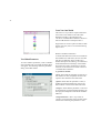
Starting Screen
Every time when you launch the GUI program,
you will see this screen popped up.
8 The eighth component is the various user-level
daemons that are run for the whole simulation
system. For example, the NCTUns 1.0 provide
RIP and OSPF routing daemons. By running
these daemons, the routing entries needed for a
simulated network can be constructed automatically.
Due to this distributed design, a remote user can
submit his or her simulation job to a specified
dispatcher, and the dispatcher will then forward
the job to an available simulation server for
execution. The server running the simulation
engine will process (simulate) the job and later
return the results back to the remote GUI program
for further analyses. This scheme can easily
support the server farm model in which multiple
simulation jobs are performed in parallel on
different server machines.
Compared to the above described “multiple
machine mode”, there is also a “single machine
mode.” In such a mode, all of these components
are installed on a single machine. Although in this
mode simulations cannot be run concurrently,
since most users have only one machine to use,
this mode may be the best mode for them.
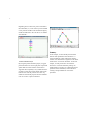
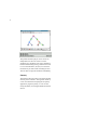
Fig. 1. The starting screen of the NCTUNS 1.0.
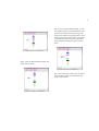
Topology Editor
The topology editor provides a convenient and
intuitive way to graphically construct a network
topology. A constructed network can be a fixed
wired network or a mobile wireless network. Due
to a user-friendly design, all GUI operations can
be done easily and intuitively.
5
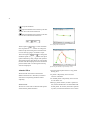
The performance monitor can easily and graphically generate and display the plots of some
monitored performance metrics over time.
Examples include a link’s utilization or a TCP
connection’s achieved throughput. Because the
format of its input data file uses the general twocolumn (x, y) format and the data is in plain-text,
the performance monitor can be used as an
independent tool; that is, it can be used to plot
graphs from data generated by other application
programs.
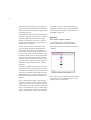
Fig. 2. The topology editor of the NCTUns 1.0.
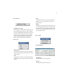
Attribute Dialog Box
A network device (node) may have many
attributes. Setting and modifying the attributes of
a network node can be easily done. Just doubleclicking the icon of the network node. An attribute
dialog box will pop up. You then can set the
device’s attributes in the dialog box.
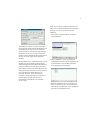
Fig. 4. The performance monitor of the NCTUns 1.0.
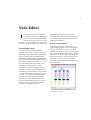
Node Editor
The node editor provides a convenient
environment in which a user can flexibly
configure the protocol modules used inside a
network node. By using this tool, a user can easily
add, delete or replace a module with his/her own
module. This capability enables a user to easily
test the performance of a new protocol.
Fig. 3. A popped-up attribute dialog box in the NCTUns 1.0.
Performance Monitor
6
Regarding how to add a new protocol module to
the node editor (i.e., to let it know you have added
a new protocol module to the simulation engine),
readers should refer to the “NCTUns 1.0 module
write manual.”
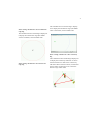
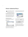
Fig. 6. The packet animation player of the NCTUns 1.0.
Summary
Fig. 5. The node editor of the NCTUns 1.0.
Packet Animation Player
By using the packet animation player, a logged
packet transfer trace can be replayed at a specified
speed. Both wired and wireless networks are
supported. This capability is very useful because it
can help a researcher visually debug and test the
behavior of a network protocol. It is also very
useful for educational purposes because students
now can see how a protocol behaves.
In this chapter, we have briefly discussed the
features and capabilities of the NCTUns 1.0
network simulator. After reading this chapter,
readers now should have a high-level view about
the NCTUns 1.0 network simulator. In the next
chapter, we will present how to install the
NCTUns 1.0 network simulator package. To
enable readers to quickly get a feeling about the
operation of the simulator, a short tour about
running a simple simulation case will be
presented.
7
Getting Started
his chapter presents a simple tour to help
readers quickly learn how to us the
NCTUns 1.0 network simulator. First, we
give instructions on how to install the
NCTUns 1.0 network simulator package on a
single machine. Next, we use step-by-step instructions to show that a user can immediately run a
simple simulation case.
T
Installation and Configuration
In the following, we assume that when installing
the package, the user uses the default settings.
A user first extracts the package from the CD or
downloads it from the web site at
http://NSL.csie.nctu.edu.tw/nctuns.html. After
reading the installation explanation and running
the installation script, a sub-directory named
“nctuns” will be created in the /usr/local/
directory, which in turn has several sub-directories. The name of these sub-directories are
“bin,” “etc,” “tools,” “BMP”, and “lib,” respectively. In the following, we will explain each of
these subdirectories.
1. /usr/local/nctuns/bin
This directory stores executable programs of the
GUI program, dispatcher, coordinator, and the
simulation engine. Their names are “nctunsclient”, “dispatcher”, “coordinator”, and
“nctunsse,” respectively.
2. /usr/local/nctuns/tools
This directory stores executable programs of
various applications and tools pre-installed by the
NCTUns 1.0 network simulator. For example,
currently “stcp,” “rtcp,” “ttcp,” “tcpdump,”
“ripd,” “ospfd,” “nctunsTcsh,” “script,” “stg,”
“rtg,” “tsetenv,” ”ifconfig,” are supported.
Due to the use of a novel kernel-reentering
simulation methodology [1], one unique
advantage provided by the NCTUns 1.0 is that any
real-life application program can run on a
simulated network to generate traffic.
During simulation, in order to run up an application program that is not pre-installed in this
directory, the user must first copy that program
into this subdirectory (i.e., /usr/local/nctuns/tools)
so that the NCTUns 1.0 can find it during
simulation. Detailed information on how to
specify which application programs should be run
on which nodes in the GUI program is presented
in the “Topology Editor” Chapter.
3. /usr/local/nctuns/etc
This directory stores the configuration files
needed by the GUI program, dispatcher, and
coordinator. Their names are “mdf.cfg,”
“dispatcher.cfg,” and “coordinator.cfg,” respectively.
4. /usr/local/nctuns/BMP
8
This directory stores the icon bmp files used by the
GUI program. These icon files are used for
displaying various devices’ icons and control
buttons.
5. /usr/local/nctuns/lib
This directory stores the libraries needed by the
GUI program and simulation engine. For example,
Qt 3.0.5 library and TCL 8.3 library need to be
installed for the GUI program and the simulation
engine, respectively.
Installation Procedure
Before starting the installation, a user should
carefully read the “README” and “INSTALL”
files first. Both of these two files contain
important installation information.
A user then runs the “install.sh” shell script. This
script will make changes to the kernel source code
of the simulation machine and then re-build the
kernel. It will also build all executable programs
and copy them to their default directories. In
addition, it will create 4,096 tunnel special files
(tunnel interfaces) in /dev. These steps may take
some time.
After these tasks are done, the machine must be
rebooted to use the new kernel. Next time when
the machine is boot up again, the whole installation is finished and can be viewed as successful.
After the installation, before using the GUI
program the first time, the user should create two
directories in his or her home directory The first
directory is .nctuns, in which several GUI
temporary files will be stored. The second is
.nctuns/etc, in which the GUI program’s
preference setting file will be stored. Note that the
creation of these two directories should be done
only once.
More detailed and up-to-date installation and
usage information can be found in the package of
the NCTUns 1.0 network simulator.
A Quick Tour
Setting up the environment
Suppose that a user uses the single-machine mode
of the NCTUns 1.0, before he (she) starts the GUI
program, he (she) needs to do three things. The
first is setting environment variables. The second
is starting up the dispatcher, and the last is starting
up the coordinator.
1. Set up environment variables:
Before a user can run up the dispatcher, coordinator, or nctuns GUI program, he (she) must first
set up the NCTUNSHOME envronment variable.
To do this, a user can type in and execute the
“setenv NCTUNSHOME /usr/local/nctuns/” shell
command in his (her) terminal window (i.e.,
xterm).
For the GUI program, an additional environment
variable LD_LIBRARY_PATH must be set. The
following shell command “setenv
LD_LIBRARY_PATH /usr/local/nctuns/lib” can
be executed to do this job.
2. Start up the dispatcher:
Now a user can run up the dispatcher, which is
located in /usr/local/nctuns/bin.
9
The default port number used by the dispatcher to
receive messages sent from coordinator
program(s) is 9,810. It is 9,800 for the dispatcher
to receive messages sent from GUI program(s).
These default settings can be found and changed
in the dispatcher.cfg file, which is located in
/usr/local/nctuns/etc/.
3. Start up the coordinator:
Now a user can run up the coordinator, which is
located in /usr/local/nctuns/bin.
After all of the above steps are successfully done,
now the user should be able to launch the NCTUns
1.0 GUI program (called nctunsclient) successfully. This program is also located in
/usr/local/nctuns/bin.
Draw a Topology
After the starting screen of the NCTUns 1.0 disappears, a user will be presented a working window
as shown below.
Since the coordinator needs to register itself with
the dispatcher, we must let the coordinator know
the port used by the dispatcher to receive registration messages. (It is 9,810 in the above
example.) This port information is specified and
can be changed in the coordinator.cfg file located
in /usr/local/nctuns/etc/.
The second important information for the coordinator to know is the IP address used by the
dispatcher. If the user is using the single-machine
mode, since the dispatcher and the coordinator are
running on the same machine, the IP address can
be specified as 127.0.0.1, which is the IP address
of the look-back network interface. On the other
hand, if a user is using the multiple-machine mode
and the dispatcher is running on a remote
machcine, the IP address specified should be the
IP address of that remote machine.
If the settings specified in the coordinator.cfg file
are all correct, then the user can start up the
coordinator now.
4. Start up the nctunsclient:
The initial working window.
To edit a new network topology, a user can
perform the following steps.
1. Choose File > Operating Mode and make sure
the “Draw Topology” mode is checked.
Actually, this is the default mode which the
NCTUns 1.0 will be in when it is launched.
10
It is important to note that only in this mode, can
a user draw a new network topology (structure)
or change an existing simulation case’s
topology. When a user switches the mode to the
next mode “Edit Property”, the simulation
case’s network topology can no longer be
changed. Instead, only devices’ properties
(attributes) can be changed at this time.
The GUI program enforces this rule because
when the mode is switched to the “Edit
Property” mode, for the user’s convenience, it
will automatically generate many settings (e.g.,
an layer-3 interface’s IP and MAC addresses).
Since the correctness of these settings depends
on the current network topology, if the network
topology gets changed, these settings will
become wrong.
If after editing some devices’ properties, the
user would like to change the network topology,
he or she will need to explicitly switch the mode
back to the “Draw Topology” mode. However,
when the mode is switched back to the “Edit
Property” mode, many settings that were
automatically generated and assigned by the
GUI program will be re-generated automatically by the GUI program. These new settings
may be different from the old settings!
For example, the IP and MAC addresses
automatically assigned to a layer-3 network
interface may have been changed. The user thus
better re-checks the settings for application
programs (traffic generator) that he (she) has
specified while he (she) was in the “Edit
Property” mode. The is because these application programs now may use wrong IP
addresses to communicate with their intended
partners.
2. Move the cursor to the toolbar.
3. Left-Click the router icon (
) on the toolbar.
4. Left-Click somewhere in the blank working
area to add a router to the current network
topology (which is empty now).
5. Left-Click the host icon (
) on the toolbar.
Like step 4, let’s add three hosts to the current
topology. The result is shown below.
11
6. Now we want to add links between the hosts and
the router. Left-Click the link icon (
) from
the toolbar to select it.
7. Left -Click some host and hold the mouse
button. Drag this link to the router. Then release
the mouse left button on top of the router.
It is not necessary to save the network topology
into a file in this mode. A user can also save it
in the “Edit Property” mode. Depending on in
which mode a network topology file was saved,
when the file is opened again, its current mode
will be automatically set to the mode when it
was saved.
8. Add the other two links in the same way. Now
our simple topology is done.
Editing Nodes’ Properties
A network node (device) may have many parameters to set. For example, we may want to set the
maximum queue length of a FIFO queue used
inside a network interface. For another example,
we may want to specify that some application
programs (traffic generators) run on some hosts or
routers to generate network traffic.
9. Remember to save this network topology by
choosing File > Save. For this simple case, we
will save the topology file as “test.tpl”.
Before a user can start editing the properties of
network nodes, he or she should switch the mode
from the “Draw Topology” to “Edit Property”
mode. In this mode, topology changes can no
longer be made. That is, a user cannot add or
delete network nodes or links at this time. If the
user has not given a name to this simulation case,
the GUI program will pop up a dialog at this time
asking the user to specify one.
As explained before, to greatly save the user’s
configuration time, the IP and MAC addresses
used by layer-3 network interfaces are automatically generated and assigned by the GUI program.
In addition, the MAC addresses used by layer-2
network interfaces are automatically generated.
Layer-3 interfaces are used by layer-3 devices
such as hosts, routers, and mobile nodes. Layer-2
interfaces are used by layer-2 devices such as
switches and wireless LAN access points.
12
The generated IP addresses use the
1.0.subnetID.hostNumOnThisSubnet format,
where subnetID and hostNumOnThisSubnet are
automatically assigned. As such, the NCTUns 1.0
network simulator can allow a simulation case to
have up to 254 subnets (subnet ID 0 and 255 are
excluded for broadcast purposes), each of which
can have up to 254 nodes (hostNum 0 and 255 are
excluded for broadcast purposes). That is, in total,
254 * 254 = 64,516 nodes can be supported in a
simulation case.
Although in theory the NCTUns 1.0 can support
this large number of nodes in a simulation case, in
practice, this is rarely done. This is because each
layer-3 interface needs to be simulated by a tunnel
interface and currently we create only 4,096
tunnel interfaces in a UNIX machine. So,
precisely speaking, currently the NCTUns 1.0 can
support any simulation case using up to 4,096
layer-3 interfaces. This means that currently the
maximum number of mobile nodes in a mobile ad
hoc network simulation case cannot excced 4,096.
(This is because each mobile node uses a layer-3
interface.)
The used subnet number starts from 1 and
automatically grows upward. The used host
number on a subnet also starts from 1 and
automatically grows upward. If there are ad-hoc
mobile nodes in the network, the subnet ID 1 is
reserved and used for the ad-hoc subnet formed by
these ad-hoc mobile nodes. In such a case, the
subnet number used for fixed subnets will start
from 2. On the other hand, if there is no ad hoc
mobile nodes in the network, the subnet number
used for fixed subnets will start from 1.
Note that the GUI program only automatically
generate and assign IP addresses to ad-hoc mobile
nodes (
),and hosts and routers on the fixed
network. For infrastructure mobile nodes (
),
the GUI program does not automatically generate
and assign IP addresses to them.
The reason is that an infrastructure mobile node
needs to use an access point to connect itself to the
fixed network. To be able to successfully send and
receive packets to and from the fixed network, the
infrastructure mobile node needs to use an IP
address whose subnet ID is the ID of the subnet
that the access point belongs to. However, during
the automatic IP generation process, the GUI
program does not know which subnet the user
would like an infrastructure mobile node to belong
to. As such, the GUI program cannot intelligently
generate and assign an appropriate IP address to
an infrastructure mobile node.
Due to the reason, this task thus must be left to the
user as his or her responsibility. Beside configuring the IP address manually, the user also needs
to manually configure the gateway IP address for
the infrastructure mobile node. Otherwise, its
packets cannot get forwarded beyond the subnet
that it is attached to. Configuring the gateway IP
address can be done in the mobile node’s dialog
box under the “Wireless Interface” tab.
A user should be aware that if he (she) switches
the mode back to the “Draw Topology” mode,
when he again switches the mode back to the “Edit
Property” mode, nodes’ IP and MAC addresses
will be re-generated and assigned to layer-3 inter-
13
faces. Therefore the application programs (traffic
generator) now may use wrong IP addresses to
communicate with their partner.
In this mode, since the IP and MAC addresses and
the port ID of an interface are already automatically generated and assigned, the GUI will
automatically show these information when a user
moves the mouse cursor and place it over the blue
interface box on the screen for a while. This can
conveniently let the user see the results of the
automatic IP and MAC address and the port ID
assignments.
Beside automatically generating IP and MAC
addresses (to save a user’s time), the GUI program
also automatically and silently perform many
tasks for the user. Many of these tasks are
performed underground to automatically correct a
user’s configuration mistakes. This is to avoid
generating wrong simulation results or even
causing simulation crashes.
For example, the GUI program will automatically
set the promiscuous mode of the 802.3 MAC
modules that are used inside a switch to ON, no
matter how the user set them. (The promiscuous
mode is default to OFF because the 802.3 MAC
modules used inside hosts and routers need to
filter out unwanted frames.) This ensures that
frames can be forwarded by the switch without
any problem. Otherwise, if the promiscuous mode
is not turned ON, frames will be discarded by the
switch’s 802.3 MAC modules.
Another task that the GUI program does for the
user is to ensure that all interfaces that connect to
a hub uses the hub’s bandwidth as their interface
bandwidth and the operating mode of these inter-
faces’ 802.3 MAC modules all be set to “halfduplex.” In the GUI program, a user can independently set different bandwidths for different interfaces and set a 802.3 MAC module’s mode to
either “full-duplex” or “half-duplex” without
considering whether these interfaces are
connected to a hub. These wrong configurations
surely will generate wrong simulation results and
may even cause crashes. This kind of misconfiguration bug is difficult to detect for a careless user.
As such, the GUI program does several underground tasks to save the user’s time and increase
his (her) productivity.
Yet another task that is automatically done by the
GUI program is that the GUI program will force
the switch module used inside an access point
(
) to use the “Run_Learning_Bridge” mode,
despite that the user may configure it to use the
“Build in Advance.” These two modes affect how
the switch forwarding table used inside the switch
module is built. The first method is a dynamic
method while the second is a static method. The
second method works very well for fixed
networks. However, in mobile networks where
mobile nodes move around and change their
associated access points constantly, the static
method will no longer work correctly. To avoid
the user to suffer from unexpected (wrong)
simulation behavior and results, the GUI program
thus automatically forces the switch module inside
all access points to use the dynamic
“Run_Learning_Bridge” method to dynamically
build their switch forwarding tables.
14
So, in the future when you see that the GUI
program does not honor your settings for some
devices or protocol modules, do not be surprised.
You know that the GUI program is doing this for
your good.
Editing network nodes’ properties can be done in
two ways. In the first way, a user can use the
mouse to double-click a network node’s icon. A
dialog box will soon appear in which a user can set
parameter values or option values. The following
shows the results of double-clicking the router
icon.
One important task in the “Edit Property” mode is
to specify which application programs (traffic
generators) will run on which nodes during
simulation to generate network traffic.
In the second way, a user can use the node editor
to specify the protocol module parameters used
inside a network node. To enter the node editor,
first a user double-clicks the node’s icon to pop up
its dialog box. Then the user double-clicks the
“node editor” button in the dialog box. The
following shows the popped node editor and the
protocol modules used by the router.
Application programs are allowed to run on hosts,
routers and mobile nodes (including both the adhoc and infra-structure modes). Therefore, in
these devices’ dialog boxes, there is an “Application” tab for a user to specify the commands for
launching the user’s desired application programs.
The following shows the Application tab.
15
uration file (.tfc). The format of a .tfc file is the
same as the .tfc file exported by the GUI program
for a simulation case when it switches its mode to
“Run Simulation.”
Normally, a .tfc file used in such a case is
generated by a script or a program written by the
user. Each traffic generator (i.e., application
program) command string specified in the .tfc file
will be put to the Applications tab of the specified
node. This operation can greatly save a lot time
because now the user need not invoke each node’s
dialog box individually. The following shows
where this command is located.
For example, suppose that a user wants to sets up
a greedy TCP connection between two nodes. He
can specify the invocation command “rtcp -p
8000” on the receiving node’s Application tab and
specify the command “stcp -p 8000 1.0.1.2” on the
sending node’ Application tab. In this case, rtcp
and stcp are the pre-installed application programs
that greedily send and greedily receive TCP data,
respectively. Also, we assume that the receiving
node has an assigned IP address of 1.0.1.2 and the
rtcp program binds its receiving socket on port
8000.
From the above example, we see that the specified
invocation commands are exactly the same as a
user would type in a UNIX terminal to invoke (run
up) these application programs by himself/herself.
For a large network that has hundreds or
thousands of nodes (hosts, routers, or mobile
nodes), the user can use the GUI’s /Tools/Insert
Applications/ command to read in a traffic config-
Running the simulation
When a user finishes editing the properties of
network nodes and setting up application
programs, he or she can start to run the simulation.
In order to do so, the user must switch the mode
explicitly from “Edit Property” to “Run
Simulation.” Entering this mode indicates that no
more changes can (should) be made to the
simulation case, which is reasonable. The
simulation is about to be started. At this moment,
of course any of its settings should be fixed.
16
Whenever the mode is switched into the “Run
Simulation” mode, the simulation files that
describe the simulation case will be exported.
These simulation files will be transferred to the
(remote or local) simulation server for it to
execute the simulation. These files are stored in
the “mainFileName.sim” directory, where
mainFileName is the name of this simulation case
chosen in the “Draw Topology” mode.
For example, if the topology file is named
“test.tpl,” these exported simulation files are
stored in a directory named “test.sim.” Among
these exported files, the test.tcl file stores the
configuration of every node’s protocol stack. This
file is very important and should always goes with
the test.tpl file. For example, if a user wants to
move (or copy) a simulation case from one place
to another place in a file system, he (she) must
move (or copy) the .tpl and .tcl files at the same
time. Otherwise, the moved (or copied) simulation
case cannot be successfully reloaded. For this
particular example, he (she) must move test.tpl
and test.sim/test.tcl at the same time.
Beside the “.sim” directory, a directory named
“mainFileName.results” is also created. This
directory will store the generated simulation
results when they are transferred back to the GUI
program after the simulation is done.
It is important to note that before a user runs a
simulation case, he or she can still switch the
mode back to the “Edit Topology” or even the
“Draw Topology” mode to change any setting of
the simulation case. However, when the mode is
switched back into the “Run Simulation” mode,
all simulation files will be re-exported to reflect
the most recent settings.
Before a user runs a simulation, he or she must
make sure that the dispatcher and coordinator are
already running. Suppose that the user uses the
single-machine mode of the NCTUns 1.0, he (she)
will have to run up the dispatcher and coordinator
programs first. The following procedure assumes
that the user uses the “single-machine” mode. If
the user uses the multiple-machine mode to use a
simulation service center that is already set up by
some person or institute, he (she) can skip the
following two steps.
1. Run the “dispatcher” program located in
/usr/local/nctuns/nctuns/bin
2. Run the “coordinator” program located in
/usr/local/nctuns/bin. The default values of the
parameters needed by this program is stored in
/usr/local/nctuns/etc/coordinator.cfg.
Now we need to let the GUI program know the IP
address and port number used by the dispatcher.
The user should configure these settings by
invoking the Setting > Dispatcher command. The
following shows the popped-up dialog box.
17
Since we have made a complete simulation case
and we are sure that the dispatcher and coordinator
are ready, we can now proceed to run the
simulation.
1 Choose File > Operation Mode. And check
“Run Simulation”.
The default port number is 9,800. If the user is
using the single-machine mode, the IP address can
be specified as 127.0.0.1. The user name and
password must be valid. For the single-machine
mode, they are the user’s account on this local
machine. For the multiple-machine mode, they are
the user’s account on the remote dispatcher
machine.
During simulation (i.e., when the simulation is not
finished yet), the result files generated by the
simulation engine are stored in the home directory
of the provided user account. Hence, this information must be correct and valid. Otherwise, the
GUI program will crash due to access permission
error. Specifying the email address is not
necessary. However, if this information is
provided, a remote dispatcher will send back a
notice email to the user when the user’s
background job is finished in its simulation
service center.
2 Choose Simulation > Run. Executing this
command will cause the current simulation job
to be submitted to one available simulation
server managed by the dispatcher.
3 When the simulation server is executing, the
user can see the time bar at the bottom moves.
The time bar will reflect the current virtual time
(progress) of the simulation case.
18
Playing Back the Packet Transfers
After the simulation is finished, the simulation
server will send back the simulation result files to
the GUI program. After receiving these files, the
GUI program will store these files in the “.results”
directory. It then automatically switches to the
“Play Back” mode.
To save the network bandwidth required for transferring these huge file across a network
(especially across the slow Internet), these result
files are tarred (using the tar command) and
gzipped (using the gzip command) into a tar ball
before being sent to the GUI program. This can
effectively reduce the bandwidth usage by a factor
of 10 or above. After receiving the tar ball, the
GUI program needs to untar and ungzip the tar ball
before using these files. As such, a user may
experience some delay of up to a few seconds
(depending on the machine’s speed) without any
progress update on the screen. At this moment, the
user needs to be patient.
These files include a packet animation trace file
and all log files that the user specified to generate
while in the “Edit Property” mode. The packet
animation trace file can be replayed later by the
packet animation player while the performance
curve of these log files can be plotted by the
performance monitor. Details about the animation
player and the performance monitor will be
explained in later chapters.
For this simple case, the packet animation trace
file is named “test.ptr,” which uses the main file
name of our topology file -- “test.tpl.” The .ptr is a
logged packet transfer trace file. Its animation can
be played by the animation player at any specified
speed.
When the GUI program has untarred and
ungzipped the ptr animation log file, it automatically switches to the “Play Back” mode. In this
mode, the control buttons of the time bar located
at the bottom of the screen can be used to
play/stop/pause/continue/jump forward/jump
backward/intelligently jump forward the
animation. The user can also directly move the
time knot to his/her desired time to see the packet
transfers occurring at that time.
For example, the user can left-click the start icon
(
) of the time bar located at the bottom. The
animation player then will start playing the
recorded packet animation.
The following shows these control buttons.
The following shows the animation player when it
is playing an animation log file.
19
At this stage, the whole process of using the
NCTUns 1.0 network simulator to perform a
simulation case study is over. The user may quit
the GUI program at this time while leaving the
dispatcher and coordinator program running in the
background.
Post Analyses
While the packet animation player is running, the
user can also launch the performance monitor to
plot performance curves of logged performance
metrics over time. For example, a TCP
connection’s achieved throughput or a link’s utilization. The time used by the performance monitor
and the packet animation player are synchronized
with each other. The following shows the performance monitor while it is plotting a performance
curve.
Later on when the user wants to review the
simulation results of a simulation case that has
been finished before, he can run up the GUI
program and then open the case’s topology file.
The user then can switch the mode directly to the
“Play Back” mode. The GUI program then will
automatically reload the simulation results (the
animation file and performance plotting log files.).
Because the animation file size is usually very
large, this loading process may take a while.
After the loading is finished, the user can use the
control buttons located at the bottom of the screen
to view the animation, just like what he/she would
do when a simulation job is done.
20
Simulation commands
After running up a simulation and before it is
finished, a user can have control over its
execution. Job control commands are grouped in
Menu > Simulation. The following will explain
the meaning of each job control command.
• Run: Start to run the simulation
• Pause: Pause the currently-running simulation
• Continue: Continue the simulation that was just
paused
• Stop: Stop the currently-running simulation
• Abort: Abort the currently-running simulation.
The difference between “Stop” and “Abort” is
that a stopped simulation job’s results will be
transferred back to the GUI program. However,
an aborted simulation job’s results will not be
transferred back. They will be immediately
deleted on the simulation server to save disk
space.
• Reconnect: the Reconnect command can be
executed to reconnect to a simulation job that
was previously disconnected. All disconnected
jobs that have not finished their simulations or
have finished their simulations but their results
have not been retrieved back to the GUI program
by the user will appear in a session table. When
executing the “Reconnect” command, a user can
choose a disconnected job to reconnect from this
session table.
• Disconnect: Disconnect the GUI from the
currently-running simulation job.The GUI now
can be used to service another simulation job. A
disconnected simulation job will be given a
session name and stored in a session table.
• Submit: Submit a job to the dispatcher without
first running it in the GUI then immediately
disconnecting it. Its net effect is the same as first
running a simulation job and then immediately
disconnect the GUI program from it. A job
submitted in this way is called a “background”
job. It does not need the GUI’s support (or
occupy the GUI) while its simulation is ongoing.
A background job may wait in the dispatcher’s
job queue if currently there is no available
simulation server to service this job. Whenever
a simulation server becomes available, on behalf
of the GUI program that submitted this
background job, the dispatcher will automatically start the background job’s execution on
that simulation server.
Remote File Management
If the GUI user uses the NCTUns 1.0 network
simulator’s multiple-machine mode (e.g.,
submitting his or her jobs to the simulation service
center located at NCTU), since the machine on
which the GUI program runs is different from the
machine on which the simulation server running
this simulation runs, the generated simulation
results will temporarily be stored on the remote
simulation server.
By default, the files generated on a simulation
server will be automatically deleted after they are
automatically transferred back to the GUI
program. Such a design is to save disk space.
However, in some normal cases result files may be
generated and temporarily left on the remote
simulation machine. For example, the results of a
background job that is finished are left on the
21
remote machine. In some abnormal cases , result
files can also be left on the remote machine. For
example, the GUI machine is accidentally
powered off. Due to these reasons, the GUI
program provides the File > Remote File
Management command command for a user to
clean up unused files stored on a remote server.
If the user is using the single-machine mode, the
user can also do the clean-up without executing
this command. He (she) can directly process the
files stored in the .nctuns/coordinator/workdir
located in his (her) home directory.
Background Job Management
As explained before, a background job is a job
submitted by executing the “Submit” command.
After being submitted, a background job may wait
in the dispatcher’s job queue waiting for an
available simulation server to service it, being
currently executed by a simulation server , or may
have finished its simulation. Depending on which
state a background job is currently in, a user can
use appropriate commands to either cancel it,
reconnect to it, or retrieve its simulation results.
This function is provided by the File >
Background Job Management command.
Summary
In this chapter, we present how to use the NCTUns
1.0 network simulator to quickly build a
simulation case. The package installation process
and initial environment configuration are covered
in detail. We also provide a quick tour to help
users learn how to run up his or her simulation
case right away.
In later chapters, the functions and capabilities of
the GUI program will be explained in more detail.
In the next chapter, we will begin with the
topology editor.
22
Topology Editor
uilding a new network topology is the
first step toward running a simulation.
It’s an easy job through the use of the
topology editor of NCTUns 1.0. The
topology editor not only provides friendly GUI
but also provides various attribute dialogs. The
following steps will show you how to build a
network topology quickly.
B
Four Modes in Topology Editor
Menu->File->Operating Mode->Draw Topology,
Edit Property, Run simulation, Play Back)
nodes during simulation. However, in this mode, a
user can no longer change the topology of the
network fixed in mode 1.
Mode 3: Run simulation. In this mode, a user can
run/pause/continue/stop/abort/disconnect/reconne
ct a simulation in this mode. No simulation
settings can be changed in this mode.
Mode 4: Play Back. After a simulation is finished,
the *.ptr packet animation trace file will be
automatically sent back to the GUI program. The
GUI program will then automatically enter into
mode 4.
Adding Nodes with Tool Bar
Four modes exist in the NCTUns 1.0 network
simulator. A user must switch the mode at proper
times to make the topology editor work correctly.
Mode 1: Draw Topology. In this mode, a user can
add new nodes or links. He (she) can also delete
nodes or links.
Mode 2: Edit Property. In this mode, a user can
edit the property of any node and specify the application programs that will run on some particular
There are several types of network device icons on
the tool bar, including host
, hub
, router
, switch
, access point
, mobile
node (ad hoc mode)
, and mobile node (infrastructure mode)
. A user could choose a
device for insertion by clicking the mouse left
button on it. He (she) then can move the mouse
cursor to a location in the working area and then
click again to place the chosen device on the
current position of the cursor. The following
shows the topology after a user has put some node
in the working area.
23
When nodes and links are added or deleted to form
a network topology, a node’s ID and the ID of its
ports (interfaces) will be automatically assigned
and adjusted by the GUI program. The GUI
program will re-number each node’s ID when any
node is deleted from the topology to make sure
that node IDs are continuously numbered. For a
node, when one of its link is deleted, the GUI
program will also re-number the ID of all of its
ports (interface) to make sure that port IDs start at
1 and are continuously numbered inside a node.
Of course, a network topology consists of not only
nodes but also links between them. Links also can
be added to the network topology very easily. A
user can click the link icon
, move the cursor
to one device node, click the device node to fix
one end of the link, drag the link to another device
node, then click the selected node to fix the other
end of the link. The user can see that a straight line
between the two selected nodes is established. The
following shows the topology after the user has
placed several links in the working area to connect
these nodes together.
To clearly see where a mobile node has moved to,
a node’s ID is displayed next to its icon on the
screen at all time. A port (interface) of a node is
represented by a blue box. When the user switches
the mode to the “Edit Property” mode, a layer-3
port’s IP and MAC addresses will be automatically generated and assigned. In this mode, if the
user moves the mouse cursor and place it over the
blue box for a while, the port’s information (port
ID and IP address) will be shown on the screen.
Note that the information shown for a layer-1 port
(e.g., a hub port) or layer-2 port (e.g., a switch
port) contains only the port ID information. This
because these ports do not have IP addresses
assigned to them. The above picture shows that
each interface is represented by a blue box.
In a real network environment, a mobile node has
its own moving path. To specify a mobile node’s
moving path, a user can first click the icon
on
the tool bar. He (she) then clicks the mobile node
and start dragging and dropping repeatedly to
construct its whole moving path. This operation
continues until the user clicks the mouse right
button.
24
A moving path is composed of a sequence of
turning points and segments. After a moving path
is constructed, any of its turning points can be
moved to any place to adjust the shape of the path.
Each turning point is represented by a grey dashed
square box and contains the (X-loc, Y-loc, arrival
time, pause time, speed to the next point) information. This information can be changed by
double-clicking the box. When a mobile node is
moving from one point to the next point (i.e.,
moving on a segment), its moving speed is fixed.
There are some other useful tools on the tool bar.
They are select
, delete
, ruler
,
zoom in and zoom out
. The operation of
the ruler is the same as setting up a link between
two device nodes. A message box will show up
telling the distance (in meter) between the selected
two nodes. It is primarily used to place mobile
nodes and access points at proper locations so that
their wireless signals can or cannot reach each
other as planned.
Editing the attributes of Nodes
After nodes are added, a user can enter mode 2 to
set the detailed attributes of any node by doubleclicking its icon.
Here are some common attribute tabs shared by
many kinds of devices.
Under the [Application] tab, a user can specify
which application program to run on this node. He
(she) can put the command string into the
“command” field. In addition to the command
string, the start, stop time, and argument of the
specified command program can also be set.
About the [Down time] tab, a user can set the
durations during which the node is down (cannot
send or receive any packet). The down time
periods configured here will be propagated and set
25
in the Phy (or WPhy) module of each of the node’s
interface. This is because the Phy (or Wphy)
modules are the right place to disable or enable the
transmission or reception of packets.
To turn down only an interface but not all interfaces of a node, a user can open the node’s node
editor, double click that interface’s Phy (or Wphy)
module, and then enable its “Link Failure” option
to set the down times for that particular interface.
The link property setting dialog
The down time period information will be propagated to and be set in the Phy (or Wphy) module
of the two nodes that connect to this link.
Therefore, the down time periods set in an
interface’s Phy (or Wphy) module actually is the
union of the down time of the node to which this
interface belongs and the down time of the link to
which this interface connects.
the Phy module in the node editor.
Note that a user can also set the down time periods
of a link. By double-clicking a link, a link attribute
dialog will show up. In the dialog, a user can set
the link’s bandwidth, signal propagation delay,
bit-error-rate (BER) and down time periods for
each direction of the link. The picture below
shows the link property editing dialog box.
Beside the down time information, other attributes
of a link are also propagated to the appropriate
modules of the two nodes that connect to this link.
For example, the bandwidth, signal propagation
delay, and BER are all propagated and set in these
Phy (or Wphy) modules. It is worth noting that
this automatic link parameter propagation process
will override the settings specified by the user in
the node editor for these Phy (or Wphy) modules.
The GUI program adopts this design because it is
more intuitive and natural to set a link’s attributes
by double-clicking it. Individually invoking the
node editors of the two nodes that are at the ends
of a link to set the link parameters is less intuitive
and natural.
26
[Command console] is equipped by Host, Router,
and Mobile Nodes. This function is enabled only
when a simulation is currently running. A user can
use this console to log into the current node (the
node whose dialog box is shown right now). A
xterm terminal window will appear. In this
terminal window, a user can run the tcpdump
program to capture packets passing through one of
this node’s interface.
For a router, suppose that the user wants to capture
the packets flowing through one of its interfaces.
Further assume that this particular interface is
configured with 1.0.2.3 IP address. The user can
first type in “ifconfig -a” command to find out the
information about all of the router’s interfaces.
From the output, the user can find the name of the
desired interface which is configured with 1.0.2.3.
In the NCTUns 1.0 network simulator, an
interface’s name is in the fxpXXX format, where
XXX is the interface’s port ID. After finding the
name of the desired interface, the user now can
type in the following command “tcpdump -i
fxpXXX” to launch the tcpdump program.
command console login screen
The command console is a very useful feature. A
user can also use this console to launch application
programs at run-time to generate traffic. For
example, while the simulation is running, the user
can open a sending node’s command console to
launch the “stcp -p 8000 1.0.1.2” program and
open a receiving node’s command console to
launch the “rtcp -p 8000” program, assuming here
that the receiving node has an interface configured
with 1.0.1.2.
In addition, executing the ping command in a
command console is also very useful. This is
because doing this can help a user find whether the
routing path between two nodes is correctly set up
during simulation.
Beside the above shared tabs, each device has its
own ones that will be presented below.
• Host
27
• Hub
can also be performed by clicking the “Show
routing table” button when a simulation is
running.
• Switch
Because every port of a hub must use the same
bandwidth. A field is provided here to set up the
hub’s bandwidth.
• Access Point
• Router
Under the [wireless interface] tab, a user can
examine the interface attributes (e.g., the used
frequency channel and the wireless signal transmission range).
In this dialog, a user can specify whether routers
should run routing daemons (e.g., RIP, OSPF) to
construct their routing tables or their routing
tables should be calculated in advance by the GUI
program. Run-time routing table content lookup
28
• Mobile Node (Ad hoc and Infrastructure mode)
current and next points. On the other hand, “Keep
arrival time” will calculate the needed speed based
on the arrival time of the next point and the
distance between the current and next points.
To generate random waypoint paths, two methods
are provided. A user can ask the GUI program to
generate random waypoints on the fly. He or she
can also import the path from a file. The user can
also export the mobile node’s current moving path
to a file for later uses.
Under [Single-hop connectivity] tab, the GUI
program will calculate and list when a mobile
node other than the current one can and cannot be
reached by the current mobile node in its singlehop transmission range. On the other hand, under
[Multi-hop connectivity] tab, the GUI will
calculate and list when a mobile node other than
the current one can and cannot be reached by the
current mobile node in multiple hops, through the
help of the ad doc mode forwarding. These two
functions are provided for research results
comparison purposes. This is because their results
represents the most accurate and most optimal
routing paths that only “God” can achieve at any
time.
A powerful and flexible configuration dialog box
is provided for mobile nodes.
Under [Path] tab, the moving speed, position (X,
Y) of each turning waypoint, pause time during
which mobile node stays at the current turning
waypoint can be configured.
Note that two methods of adding new waypoints
are provided here. “Keep moving speed” will
calculate the arrival time of the next point by the
current default speed and the distance between the
Advanced method to add Mobile Nodes
Beside the simple way to click the mouse to add
one mobile node at one time, there are several
other methods that can be used to add multiple
mobile nodes at one time.
Insert Mobile Nodes
29
Multiple mobile nodes that use the same protocol
stack and parameter settings could be added by a
user at the same time. This is very convenient and
efficient for a user. The following is an effective
way to add a large number of mobile nodes. The
generated mobile nodes can be placed at random
positions or can be placed in an m*n mobile node
array.
Import/Export all moving paths from/to file
It is worth reminding that before generating a
large number of mobile nodes that use a protocol
stack other than the default one, the user better
first invokes the node editor in this dialog to
specify the protocol stack used by them. If this
operation is not done before generating a large
number of nodes, the user later will suffer from
invoking all mobile nodes’ node editors to
configure their protocol stacks. This would be a
pain!
Generate Random Waypoints
This operation saves/loads mobile nodes’ moving
paths into/from a *.mdt file. It’s convenient for a
user to save mobile nodes’ current moving paths
to a file and later reload and reuse them.
There are two ways to help a user generate random
waypoints. The first one is to generate the next
waypoint randomly for each mobile node. When
the user clicks the button, one more random
waypoint will be generated for every mobile node.
The user can press the button continuously to
continuously generate more random waypoints.
The other way is to automatically generate
random waypoints until the specified time in
virtual time (e.g., 10 sec) has elapsed.
Generate Infrastructure Node IP and Mac
Addresses
This command can automatically generate IP and
MAC addresses for a large number of infrastructure mode mobile nodes. In the “Getting
30
Started” Chapter, we mentioned that the GUI
program will not automatically generate and
assign IP addresses to an infrastructure mode
mobile node because it does not know to which
subnet that infrastructure mode mobile node
should belong.
However, to save the user a lot time spent on
manually assigning IP addresses to a large number
of infrastructure mode mobile nodes, the GUI
program still provides this function here. If the
user knows to which subnet a group of infrastructure mode mobile nodes should belong (i.e.,
the subnet ID), he or she can use this function to
insert a group of infrastructure mode mobile
nodes, with their IP addresses automatically
assigned.
Note that when you want to automatically
generate IP addresses for infrastructure mode
mobile nodes, the total number of these nodes
must not exceed 255. Otherwise, the 255 IP
addresses on the specified subnet will be used up
and will not be sufficient for all of these nodes.
Remove All Moving Paths
Executing this command can delete all mobile
nodes’ moving paths. This will give the user a
clean working area to start with.
their wireless signals can reach or cannot reach
each other at particular times or at particular
locations.
To help a user do this tedious job, the ruler tool is
provided by which a user can measure the distance
between two nodes.
To further help the user, the GUI program
provides the “See Mobile Node Movement”
mode. In this mode, mobile nodes will move along
their moving paths over time and a red line
(connectivity indication) will show up between
two mobile nodes whenever their wireless signals
can reach each other. This way, the user can easily
see whether his or her mobile path configurations
really match his or her expectations.
To enter this mode, a user can simple check this
mode. Then the user can use the control buttons of
the time bar located at the bottom of the screen to
control the progress. To leave this mode, the user
can simply check this mode again.
When a mobile node starts moving in this mode, a
green box will appear on the screen to indicate its
current location. To have a clear view of the field,
the user can choose not to display these mobile
nodes’ moving paths and their icons. How to
change these settings are explained below.
Change View of the Mobile Node
Enter See Movement Mode
When studying a mobile wireless network
problem, a user usually needs to specify many
mobile nodes’ moving paths in such a way that
Menu->Setting->Mobile node->show-moving-path
flag
This command can turn on/off a flag to display/not
to display the moving path of each mobile node.
31
Menu->Setting->Mobile node->show-transmissionrange flag
This command can turn on/off a flag to display/
not to display the interference range (the default
value is 550 meters) of each mobile node.
This command can turn on/off a flag to display/not
to display the transmission range (the default
value is 250 meters) of each mobile node.
Menu->Setting->Mobile node->show connectivity
flag
Menu->Setting->Mobile node->show interference
range flag
This command can turn on/off a flag to display/not
to display the connectivity indication. A shown
red line between two nodes is the connectivity
indication. When a red line is shown, it means that
the two nodes connected by it are in the transmission range of each other.
32
Menu->Setting->Mobile node->show mobile-node
flag
Files generated at remote simulation servers can
be retrieved or deleted by this function.
This command can turn on/off a flag to display/not
to display the mobile node’s icon. Doing this can
clean the working area.
Menu->File->Background Job Management
Menu->Setting->connectivity color
This command sets the color used by the connectivity indication line. Each different frequency
channel can use a different color. During a
simulation, different mobile nodes may be
configured to use different frequency channels.
Using different colors for different frequency
channels enables a user to easily distinguish them.
Any background job submitted to the dispatcher
can be manipulated here. They can be deleted,
stopped, aborted, or retrieved.
Setting the simulation
Menu->Setting->Dispatcher
Menu->Setting->wireless Frame color
This command sets the colors used by various
wireless frames. Each different frequency channel
can have a different color scheme. This is useful
when the packet animation player is running.
File manipulation
the dispatcher setting dialog
Menu->File->New
Close the current simulation case and clear the
working area for a new case.
Menu->File->Open(, Save, Save as)
Save the current simulation case’s topology and
node configurations into the .tpl and .tcl file,
respectively. This case can later be reloaded.
Menu->File->Print to File
The graph shown on the screen can be saved to a
*.bmp file for printing purposes.
Menu->File->Remote File Management
This dialog sets up the IP address and port number
used by the dispatcher. The GUI user’s login
account and password for using the remote
simulation server should also be entered here. It is
VERY important that the account name of the
GUI user used on the local GUI machine and that
used on the remote simulation server should be
exactly the same. Otherwise, the network
simulator cannot work correctly. For the singlemachine mode, the user name specified here
MUST be the same user account name by which
the user logs into this local machine. Otherwise,
the simulation cannot run correctly.
33
If the user is using the single-machine mode, the
IP address entered here can be 127.0.0.1 (the IP
address of the loopback interface) and the port
number must be the same as the CLIENT_PORT
specified in the dispatcher.cfg
Menu->Setting->Simulation
the simulation setting dialog
Under [Simulation] tab, the total simulation time
in virtual time and the maximum of X,Y,Z coordinates should be specified.
Under [GUI] tab, the ratio of meter/pixel can be
specified.
Under [Speed] tab, the tick time and simulation
speed can be specified. Note: The GUI user is
discouraged to change these settings. Right now,
for the beta version, only the “As Fast As
Possible” mode is supported.
34
Under [System command] tab, to-be-executed
system commands and their output file names can
be specified here. A system command is a
command that, when executed, will get or set an
object’s value at a specified time. The output of
the command will be saved to the specified output
file, which will later be transfered back to the GUI
program when the simulation is finished.
In addition to getting/setting a single object’s
value, the values of all objects of the same kind
can be get or set at the same time to take a global
snapshot of the network. For example, this
function can be used to take the snapshot of the
current routing tables of all routers. This global
snapshot information can help a researcher study
the convergence of a routing protocol.
Time: the starting time for triggering this
command
Command: the system command string
Output file name: the name of the output file
The system commands provided by the NCTUns
1.0 network simulator are listed below. Their
syntax and meanings are also presented below.
Set: set a value to a variable in a module
Set {node} {port} {module} {tag} {value}
Get: get the value of a variable from a module
Get {node} {port} {module} {tag}
GetAll: like Get, but get the requested variable’s
value from the same modules used in all ports of
all nodes
GetAll {module} {tag}
Note that a tag is a string associated with a
particular variable declared and used in a protocol
module. A variable here can be a single-value
variable (e.g., a FIFO queue’s maximum queue
length) or a multi-column multi-row table (e.g., a
switch table that has multiple [IP address, MAC
address] mapping entries). It is the protocol
module developer’s job to write a command()
function in his (her) module to recognize a tag and
get/set the value of its corresponding variable.
More information about the get/set command can
be found in the “Module Developer Manual.”
35
Running the simulation
A user can directly submit a simulation job to the
dispatcher for execution. Its effect is the same as
first running up the simulation and then immediately disconnecting the GUI from the just
launched simulation job.
Playing back the Packet Animation
Handle animation by Tool Bar at the bottom
the simulation command list
Menu->Simulation->Run(, Pause, Continue, Stop,
Abort)
After a user switches to mode 3, the user can start
running the simulation by executing commands in
this group.
NCTUns 1.0 has a convenient way to handle the
progress of a simulation. These job control
commands are “Pause“, “Continue”, ”Stop”,
”Abort.”
Menu->Simulation->Reconnect(, Disconnect)
A user can disconnect the GUI from a currentlyrunning simulation job. Doing this allows him
(her) to quit the GUI program to do other things.
He (she) can come back later, restart the GUI
program, and then reconnect to the disconnected
simulation job.
Menu->Simulation->Submit
When a simulation is completed, the GUI system
automatically enters mode 4. In this mode, the
toolbar at the bottom can control the progress of
the play of a packet animation trace.
The 20fps (frames-per-sec) selection box can
control the displayed animation quality. The
100% selection box can control the display speed
of the animation. To speed up the animation, a
user can set it to 1000% or a larger value.
The knot of the time bar can be dragged to any
location to jump directly to a desired time. When
the time bar is moving, all the control buttons have
their own functions.
36
The packet animation player can be used as an
independent tool. If a user wants to see the
animation of a simulation case whose simulation
had been finished long time ago and does not want
to re-run the simulation, he (she) can switch the
mode directly to mode 4 after reloading the case.
The user then can play the animation immediately.
Summary
The topology editor provides a user with a friendly
and easy-to-use interface. Through this interface,
a user can build network topologies and specify
application programs quickly. A user can also
easily add, delete, and configure different network
devices.
37
Node Editor
he node editor provides a convenient
environment for flexibly configuring the
protocol modules used inside a network
node. By using this tool, a user can easily
add, delete or replace a module with his/her own
module to test the performance of a new protocol.
T
Protocol Module Concept
A protocol module usually implements a
particular protocol such as ARP or a particular
function such as the FIFO packet scheduling discipline. In the node editor, all modules that are
grouped in the same module group (displayed at
the top of the node editor) share similar properties.
For example, in the 802.11 MAC group, we may
have one module called “802.11MAC” while
another may be called “my802.11MAC.”
Detailed information on how to add a new
protocol module to both the simulation engine and
the node editor is documented in the “NCTUns 1.0
Moduel Writer Manual.”
Screen Layout Explanation
The following will briefly explain the screen
layout of the node editor. To see the node editor,
in the topology editor a user first switches the
mode to the “Edit Property” mode by checking the
File > Operation Mode > Edit Property command.
Then he (she) can double-click a node that he (she)
wants to edit. After the node’s dialog box shows
up, the user can then press the “Node editor”
button to invoke the node editor to edit that node’s
protocol modules.
The NCTUns 1.0 network simulator provides
several pre-developed protocol modules. Users
can add new protocol modules to the node editor
or replace some existing modules with his or her
own ones. For example, in the PSBM (packet
scheduling and buffer management) module
group, three modules (FIFO, Random-EarlyDetection, Deficit-Round-Robin) are currently
supported. A user may add one new PSBM
module such as the RIO module to it.
The node editor screen shot
38
At the top of the node editor are various module
groups. The protocol modules that share the same
role in a protocol stack are grouped together under
the same group name.
In the middle working area, the protocol modules
used by this node will be shown. Here, a chain of
protocol modules represent the protocol stack
used by a port (interface). The user can use the
mouse to easily add, delete, or replace protocol
modules in the working area.
At the bottom are several control buttons. The
“Cancel” button discards all changes that have
been made to this node’s protocol modules. The
“OK” button accepts all of the changes made so
far. The “Undo” button removes the effect of the
last delete operation. (Note: only the LAST delete
operation can be undone.) The “Redraw” button
re-layouts the protocol modules so that they look
nice when shown on the screen. (This is particular
useful after a user performs the insert or delete
operation.)
The Copy-To-All-Port (CTAP) button copies the
values of the currently selected module’s parameters to the same modules in all ports of this node
The Copy-To-All-Node (CTAN) button does the
similar job. However, it copies the values to the
same modules in all ports of all nodes in the whole
network.
The “X” button means “delete.” After pressing
this button, now the node editor’s mode enters the
“delete” mode. From now on, whenever the user
uses the mouse to left-click a module or a link, that
object will be deleted. The “Arrow” button means
“select.” After pressing this button, now the node
editor’s mode enters the “select” mode. From now
on, the user can move a protocol module to any
desired place. The user can also choose a module
from the top module groups, insert and place it in
the middle working area.
Operations
Insert / Delete / Replace a module
As an example, here we demonstrate how to
replace a FIFO module with a RED module.
Step 0: The initial protocol module chain is shown
as follows.
Step 1: Then we choose the RED module from the
top and place it in the middle working area. The
resulting screen is shown below.
39
Step 4: Then we link modules together. To link
two modules together, a user performs the same
operation as he (she) does when placing a link
between two nodes in the topology editor. At the
top and bottom of a module, there is a small box.
A link must start and end on these small boxes.
After linking up modules, the result is shown
below.
Step 2: Then we delete the FIFO module. The
result is shown below.
Step 5. Since the job is finished, now we redraw
the node editor to make it look beautiful. The
result is shown below.
40
Create Your Own Module
The NCTUns 1.0 provides a simple method for a
user to add a new module to the node editor.
Detailed procedure is documented in the
“NCTUns 1.0 Module Writer Manual.” Here let’s
take the ARP module to briefly describe it.
Suppose that we want to replace the built-in ARP
module with ours, then we can use the following
steps to do it.
Define a module’s Parameters
View Module Parameters
To view a module’s parameters, a user can doubleclick a module. Then, its module parameter dialog
will appear. The following shows the parameter
dialog of the ARP module.
To let the node editor know that a new module has
been added to the node editor, the user must add
and place the definition of the module into a
module description file (mdf.cfg). To understand
the detailed format and meanings of the module
description file, readers should refer to that file
stored in /usr/local/nctuns/etc and the “NCTUns
1.0 Module Writer Manual.”
(1) parameter attribute
“local”: means that this parameter is used only in
this module. Its value, if updated, should not be
copied to other modules of the same kind.
“global”: means that this parameter’s value, if
updated, should be automatically copied to all
other modules in the network of the same kind.
“autogen”: means that the parameter’s value will
be automatically generated and determined by the
GUI program. Examples include the IP and MAC
addresses.
“autogendonotsave”: this is very similar to
“autogen” except that there will be variable substitutions when evaluating the parameter’s value.
41
Beside, since its value is automatically generated
based on a formula, any change made by the user
will not be saved.
(2) $CASE$ , $NID$ , $PID$ variable substitution
Normally, an autogendonotsave parameter’s value
is a formula consisting of the following variables.
$CASE$: will be replaced with the main file
name. For example, if a simulation case’s
topology file is saved as “test.tpl”, then $CASE$
will be replace with “test.”
$NID$: will be replaced with the ID of the node to
which this module is attached.
$PID$: will be replaced with the ID of the port to
which this module is attached.
When the parameter’s value is evaluated, variable
substitutions will occur.
Example:
Suppose that the saved topology file name is
testArp.tpl. Further suppose that an ARP module
is in a node with ID being 5 and in a port with ID
being 1. Suppose that a user sets the ArpTableFileName to “$CASE$.N$NID$_P$PID$.arp
autogendonotsave”. Then when this parameter is
evaluated, its value will become
“testArp.N5_P1.arp.” The value of a parameter of
this kind will always be automatically regenerated by the GUI program. A user cannot
change its value and save it.
Summary
In this chapter, we present the concept of protocol
modules and the node editor. The node editor is an
environment in which a user can flexibly
configure the protocol stack and parameter values
used inside a node. The NCTUns 1.0 network
simulator provides some pre-built protocol
modules. A user can add his or her own protocol
module to the node editor to test its performance.
42
Packet Animation Player
fer a user’s simulation job is finished, the
generated simulation results will be
automatically transferred back to the GUI
program and then saved in the user’s
local hard disk. Suppose that the simulation case’s
topology file is named “test.tpl.” Then the name of
the resulting packet animation trace file will be
“test.ptr.” Later, when the user wants to do post
analyses about the simulation results, he or she
can use the “Packet Animation player” to play
back the animation. This is a very useful feature
for both educations and research purposes.
A
usually very large, this process may take a while.
To give the user an idea of the progress, a progress
bar will be shown during the loading process.
status window for loading a packet
animation trace file
Reloading Simulation Results
To watch a previously generated packet animation
trace, a user should open its corresponding
topology file first.
After the animation trace file is loaded, the user
then left-clicks the start icon (
) of the time bar
located at the bottom. The player will then start
playing back the logged packet transfer animation.
menu > file > open
Some control button icons of the time bar.
General Options for Packet Animation
The user then switches to the “Play Back” mode.
The GUI program then will automatically reload
the simulation results (including the packet
animation trace file). Since the animation file is
During the play of a packet animation trace, a user
can change some options of the GUI program to
suit their needs. These options are described
below.
43
Time Bar
The time bar contains icons and buttons related to
packet animation. Now we will examine every
function from left to right.
Current simulation time timer
This timer icon shows the current simulation time.
By double-clicking the icon, a user can set the
timer to any desired simulation time. This feature
is very useful when the traffic is sparse. This is
because the user does not need to wait a long time
before seeing packet transfers. Instead, the timer
can go directly to any interesting time. Of course,
to know at what time there is a packet transfer in
the log file, the user needs to peek into the trace
file. There is a utility program (printptr) that can
convert a binary packet animation trace file into a
text trace file for this purpose. This program is
located in /usr/local/nctuns/tools.
Simulation time-bar
The time bar shows the packet animation progress
in a period between two times, called a time
window. Users can drag the time bar knot to any
desired time. Two icons are provided here to
change the size of the time window by a factor of
10. That is, the time window size can be either
increased 10 times larger or decreased 10 times
smaller. A user can conveniently perform this job
by left-clicking the time-plus icon (
) or the
time-minus (
icon).
Right at the bottom of the time bar, a red vertical
line (
) indicates that a wired packet transmission starts at this time. In a similar way, a
green vertical line (
) indicates that a wireless
packet transmission starts at this time. Note that
the ending times of packet transmissions are not
depicted here. Therefore. it may cause difficulty if
a user wants to move the time knot to the time
when a packet transmission exactly ends. Thus,
these vertical lines are depicted here for reference
purposes only.
To know exactly when a packet transmission
starts and ends, a user can use the printptr utility
program to convert the binary animation trace file
into a text file and then search it in the file.
Animation playing buttons
Animation playing buttons are provided to alter
playing sequences. They can be executed by leftclicking their corresponding icons.
(
) plays the animation. If a user clicks it while
the animation player is idle, the player will start to
play the simulation trace. If a user clicks it while
the animation player is already running, the time
bar knot will jump directly to the nearest time
where there is a packet transmission. This feature
is very useful when the traffic is sparse.
(
) pauses the animation.
44
(
) stops the animation.
(
) skip the animation time window by one time
window size in the forward direction.
(
) skip the animation time window by one time
window size in the backward direction.
successful packet transmissions
The first option (
) is to alter the frame
rates of packet animation. Users can change the
frame rate by left-clicking the increase/decrease
icons or directly typing in a number as input.
The second option (
) is to change the
animation speed. Using a larger value will speed
up the animation by using a larger time quantum
when advancing the time. However, more packet
transfers will not be displayed. This is because the
packet transfers that occur during the time leap
will not be displayed.
packet drop & collision (represented by cross)
Animation Effects
1 A link is painted yellow if there is any packet
Wired network and wireless network have
different characteristics. Therefore, we demonstrate their corresponding animation effects
separately.
2 A packet is depicted by an arrow with a
flowing on it.
“DATA” annotation.
3 A collided packet is depicted by an arrow with
an cross mark on it.
4 During a packet transfer, If a link is painted in
Wired Network
We use two screen shots to illustrate and explain
wired network packet animation.
red, it means that this link is an intermediate link
for this packet. In contrast, if this link is painted
in yellow, it means that either the source of this
45
link is the real source/destination of the packet,
or the destination of this link is the real
source/destination of the packet.
5 The arrow length is determined by the packet’s
packet length. Therefore, a user can expect that
the arrow length is proportional to the packet
length. In fact, a packet’s arrow length on a
particular link is determined by the transmission
time of that packet on that link relative to the
signal propagation delay of the link.
Wireless Network
Similarly, two screen shots are given as
illustrations.
Wireless transmission (IEEE 802.11 ACK frame)
1 Two concentric circles are centered around a
transmitting node. The smaller circle stands for
the “transmission range” while the larger one
stands for the “interference range.” Within the
interference range, a station can sense the
existence of other nodes’signals. However, only
when the receiving station is within the transmission range of the sending node, will the
packets be guaranteed to reach the receiving
station successfully.
2 A data packet is depicted by an arrow with a
“DATA” annotation.
3 An acknowledgement packet is depicted by an
wireless packet transmissions (IEEE 802.11 DATA frame)
arrow with a “ACK” annotation.
46
Summary
This chapter presents the “Packet Animation
Player” capability of the GUI program. Relevant
options are covered and some animation effects
are illustrated and explained in detail.
47
Performance Monitor
erformance monitor is a useful tool that
graphically generates and displays graphs
of some performance metrics. It can help
users monitor a links’ utilization or a
TCP connection’s throughput. This chapter gives
an overview of the functions that the performance
monitor provides.
P
corresponding performance curves over time.
Note that the performance monitor can be used as
an independent tool without the animation player
running up. That is, it can read a log file generated
by any other application program as long as the
log file uses the common (X, Y) format.
Operations for Performance Monitor
Running Performance Monitor
Choose Tool > Plot Graph. This will launch the
performance monitor’s window.
Many operations are provided in the menu of the
performance monitor window. Here we will give
a full description.
Menu -> File
• New
performance plot window
From the performance monitor window, choose
File > Open. Then a user can select a desired log
file to open.
The user then can left-click the start icon (
) of
the time bar. As the packet animation proceeds,
the performance monitor window will display the
Open a new graph window. Up to six graph
windows can be shown on the screen at the same
time.
48
This option is to pop up the snapshot window for
capturing the content that is currently displayed
in the window.
• Open
This option is to open a desired log file as a
graph source. A graph source will then be
associated with a graph window.
This window will show the captured snapshot.
Pressing “Re-snapshot” button will re-capture
the performance curve that is being displayed.
Pressing “Save” button will save the snapshot as
an image file of the “bmp” type. Pressing
“Cancel” will quit the window.
• Snapshot All
• Snapshot
This option will take snapshots of all existing
graph windows. The feature is very useful for
comparing different performance metrics’
results.
• Quit
This option will quit the current graph window.
49
Menu->Window
• Grid
This option is to select a color from the palette
and set it as the color of grids of the current
graph window.
• Graph
• Add/Remove Graph
This option is a sub-menu from which a user can
choose different graph sources. Selected graph
sources are headed with check marks. Users can
use this option to display more than one graph
sources in the same window. It is particularly
useful for comparing different performance
metrics that are collected at the same time.
This option is a sub-menu from which users can
choose a different graph source to display. Then
the user can select a color from the palette and
set it as the color of the performance curve in the
current graph window.
Menu->Option
Menu->Color
• General Setting
• Background
This option is to select a color from the palette
and set it as the background color of the current
graph window.
• Axis
This option is to select a color from the palette
and set it as the color of axes of the current graph
window.
Graph Title:
This field sets the title of the graph.
Y label:
This field sets the label of the y axis.
50
• Global Setting
X label:
This field sets the label of the x axis.
(Note that a performance curve’s label and color
can be easily set by double-clicking the curve’s
label located at the upper right corner. For
example, a user can double-click the “graph X”
default curve label.)
This option associates a graph source with a log
file. Up to six associations can be specified in
this dialog. To select a log file from the local
host, a user can press the “Browse” button.
Y tics:
This field sets the interval of the y axis.
X tics:
This field sets the interval of the x axis.
Y min:
This field sets the minimum value of the y axis.
Y max:
This field sets the maximum value of the y axis.
Show grid:
This field sets whether the grids should be
visible.
Line-Points:
Specify that the performance curve should be
drawn using straight lines to connect adjacent
points.
State-Transition:
Specify that the performance curve should be
drawn using horizontal lines to connect adjacent
points.
X-axis width
Specify how many seconds’ data should be
displayed in this graph window.
• Graph Mode
This option controls how to display a performance curve. Currently there are two modes.
The first mode is line-points while the second
51
mode is “state transition.” The following two
screenshots clarify the differences between
these two modes.
Summary
This chapter is about “Performance Monitor.” The
functions and relevant settings of the performance
monitor are discussed. Users can make good use
of this tool to help them analyze performance
results. Users can also easily take interesting
snapshots of some performance curves to make
reports.
52
Inter-Process Communications
nter-process communication enables the
NCTUns GUI to connect to both the
dispatcher and the simulation engine. We
detail how to use the facilities provided
by inter-process communication in this chapter.
I
Preparation
• Connect to the Dispatcher
Before submitting a job to the simulation enigne,
a user should check whether he (she) has correctly
set the information about the dispatcher. A user
can do this job by executing the Setting>Dispatcher command. The configuration dialog
box is shown in Fig 1.
has an IP address (say 140.113.1.1) assigned to
one of its interfaces, that IP address can be typed
in here. The user name and password should be the
same ones as those that the user uses to log in to
the local machine. If the user would like to use the
simulation service center located at the Network
and System Lab (NSL), NCTU, he (she) needs to
obtain his (her) username/password by registering
with the NCTUns web site at
http://NSL.csie.nctu.edu.tw/nctuns.html.
The default port number is 9800. A user can
modify this number by editing the configuration
file at “$NCTUNSHOME/etc/dispatcher.cfg” and
restarting the dispatcher.
Currently, the email field in the dialog box is
optional. In the future version of the NCTUns, this
information will be used by the dispatcher to send
back a job-finished notification email to the user.
• Switch to Run Simulation Mode
Fig 1. The dispatcher dialog box
If the user is running a simulation engine on the
local machine, the IP address can be 127.0.0.1,
which normally is the IP address assigned to the
loopback interface (lo0). Of course, if the machine
When the network topology and the properties of
the network are set, a user can choose to run the
simulation on-line or submit it as a background
job. Before he (she) can do that, he (she) needs to
switch the GUI mode to the “Run Simulation”
mode. The user can do this by executing File>Operating Mode->Run Simulation as shown
in Fig 2.
53
• Run a Simulation
Fig 2. Switch to the “Run Simulation” mode
Basic Simulation Operation
With the friendly GUI design, it is very easy to run
a network simulation. Most of the commands
needed are located in the “Simulation” menu ( see
Fig 3.). We will explain the usage of each of these
commands in the following sections.
After switching to the “Run Simulation” mode, a
user can submit his (her) job to a simulation server
by executing the Simulation->Run command.
Three different outcomes may be possible after
the command is executed. In the first outcome, the
simulation is submitted successfully. In this case,
the user will see the time bar located on the bottom
left start ticking. In the second outcome, a “Log in
Failed” message box will be shown up ( see Fig
4.), which means that the provided user name and
password are wrong and thus do not allow the user
to log in to the local machine. In the third
outcome, a “No idle server” message box shows
up ( see Fig 5.). This means that, currenly all of the
simulation servers are all busy executing
simulation cases. The user can try to re-run this
simulation case at a later time. He (she) can also
choose to submit it as a background job, which
will then be queued at the dispacther waiting for
its turn.
Fig 4. The “Login Failed” message dialog.
Fig 3. the Simulation menu
54
immediately. The current results will be transferred back to the GUI program for further
analyses.
• Abort a Simulation
Fig 5. The “No Idle Server” message dialog
box.
• Pause a Simulation
When a simulation is running, a user can pause it
by executing the Simulation->Pause command.
The simulation engine process and all traffic
generator processes will then be paused immediately.
When a user aborts the simulation by executing
the Simulation->Abort command, the simulation
engine and all traffic generator processes will be
killed immediately. The current results will be
completely deleted without being transferred back
to the GUI program. It is recommended that a user
either aborts or stops a running simulation before
quiting the GUI program. Otherwise, the currently
running simulation will keep running and full
results will be generated on the disk. This will
only unnecessarily waste CPU cycle and disk
space resources.
• Resume a Simulation
Session Management
A user can resume a paused simulation job by
executing the Simulation->Continue command.
The simulation engine process and all traffic
generator processes will be waked up and
continue the job from the point where you paused
it.
Most modern GUI program uses the MDI
(multiple document interfaces) design.
However, the NCTUns GUI program uses the
SDI (single document interface) design. To run
multiple simulations concurrently using a
single NCTUns GUI program, the GUI
program uses a session management
mechanism, which is discussed below.
• Stop a Simulation
Sometimes, a simulation run may take too long
and a user may thus want to retrieve the current
results before the simulation is finished. To do so,
the user can execute the Simulation->Stop
command. The simulation engine and traffic
generator processes will be stopped and killed
• Disconnect
After a simulation is run, a user can make it as a
session by executing the Simulation>Disconnect command. A session is defined to be
a simulation job that currently does not own the
55
GUI program. As such, the user can no longer use
the GUI program to control the execution of the
simulation. For a session to re-own the GUI
program, the user must execute the Simulation>Reconnect command.
After the Simulation->Disconnect command is
executed, an input session name dialog will show
up and prompt the user to input a session name
(see Fig 6.) After the session name is entered, all
information about this session is automatically
recorded by both the dispatcher and the GUI
programs. The simulation currently running on the
server side will continue its execution. However,
the user now is free to use the GUI program to
handle another simulation case. Due to this
feature, a user can run as many simulations as he
(she) wants at the same time, provided that there
are enough simulation servers in the server farm.
To avoid session name conflicts, a user should
give each session a unique name.
Fig 6. The “Disconnect” dialog box.
• Reconnect
A user can reconnect a disconnected session by
executing the Simulation -> Reconnect ->
“Session Name” command (see Fig 7.). The
session name chosen here is the name that the user
entered when he (she) disconnected the session
(Fig 6.). After the user reconnects a session, one of
two different cases may happen. In the first case,
the simulation is still running. Every soon, the user
will see the time bar resumes ticking as if the user
have never disconnected the simulation. In the
second case, the simulation is already finished
before the user reconnects it. In this case, file
transfers will automatically be started to transfer
the result and log files back to the GUI program.
Fig 7. The “Reconnect” session dialog box.
56
Background Job Management
Background job management is a useful facility
that allows a user to submit several simulation
jobs almost at the same time. A background job is
a simulation job that does not intend to use the
GUI program. After a simulation is submitted as a
background job, it will be sent to the dispatcher
program immediately and the GUI can be immediately used by other simulation cases. Thus, a user
can submit a background job without waiting for
the job to finish. It is very useful when running a
time-consuming network simulation.
Fig 8. Submit a background job
• Submit a Background Job
• Background Job Management
It takes three easy steps o submit a simulation as a
background job. First, a user needs to open/edit a
network topology and switch to the “Run
Simulation” mode (see Fig. 2). Second, the user
then executes the Simulation->Submit
command. Third, when the submit dialog box
shows up, the user then enters a desired job name
and press the “Submit” button (see Fig. 8). The job
will then be sent to the dispatcher and stored in the
dispatcher’s job queue. Immediately when any
simulation server in the server farm is available,
the first background job in the job queue will be
dispatched by the dispatcher to that server to run
the simulation.
After several background jobs are submitted, a
user can manage these background jobs through
the background job management window (see Fig
9). To pop up the window, a user can execute the
File-> Background Job Management command.
In the window, a user can easily check the current
status of his (her) background jobs. To get the
most updated information, a user can press the
Refresh button on the upper left. To close the
window, a user can press the Cancel button on the
upper right.
A background job may be in one of three different
possible statuses. First, the simulation job is
finished. In this case, the user can click on the job
name and then press the Retrieve button at the
button of the window to transfer the log files back
to the GUI program. Second, the job is currently
running on a simulation server. In this case, the
user can reconnect, abort or stop the simulation
by pressing the corresponding buttons. These
57
operations do the same thing as those described in
previous sections. Note that internally a
backgound job is processed like a disconnected
session. As such, it is possible for the GUI
program to reconnect to a background job. Third,
the job is still in the job queue waiting for
execution. The user can delete it from the job
queue if he (she) no longer wants the job to be run.
This operation can be done by pressing the Delete
button. Note that a user has to select a background
job from the table before he (she) can perform any
management operation on it. The command
buttons that are allowed for the selected job will be
enabled.
Fig 9. The “Background Job Management”
window.
Remote File Management
• Remote File Management
The remote file management utility is a convenient tool for a user to manage his (her) files that
are generated and stored on a remote server. Note
that when a user is using the “single-machine”
mode of the simulator, generated files actually are
stored on the local machine’s disk. However, the
remote file management utility can still be used
correctly.
To pop up the remote file management window, a
user can execute the File->Remote File
Management (see Fig. 10) command. The file
management window is like a file browser on
Windows operating systems. A user can change to
a directory by “double clicking” on the desired
directory name. To transfer a file from the remote
machine to the local machine, a user can simply
click on the file and press the Get button. A user
should specify the local directory to store
downloaded files. This can be done by editing the
Dir Name text field. To delete a file on the remote
server, a user can click on the file and press the
Delete button. Finally, a user can close the
window by pressing the Cancel button.
58
Fig 10. The “Remote File Management”
window.
Summary
This chapter is about “Inter-Process Communication.” The NCTUns 1.0 network simulator uses
a distributed architecture to support remote and
concurrent simulations. As such, an “InterProcess Communication” mechanism is needed to
connect all components together. In the chapter,
many commands that are related to controling the
execution of simulations are presented.
59
References:
[1] S.Y. Wang and H.T. Kung, “A Simple
Methodology for Constructing Extensible
and High-Fidelity TCP/IP Network
Simulator,” IEEE INFOCOM’99, March
21-25, 1999, New York, USA.
60