Download USER MANUAL - University of Melbourne

MPNet
Program for the Simulation and Estimation of
(p*) Exponential Random Graph Models for
Multilevel Networks
USER MANUAL
Peng Wang
Garry Robins
Philippa Pattison
Johan Koskinen
Melbourne School of Psychological Sciences
The University of Melbourne
Australia
June, 2014
Table of Content
Introduction __________________________________________________________________ 4
Acknowledgements__________________________________________________________ 4
System Requirements _______________________________________________________ 5
Setup MPNet _________________________________________________________________ 5
MPNet sessions _______________________________________________________________ 5
Start MPNet __________________________________________________________________ 6
MPNet main user interface ______________________________________________________ 7
Simulating one-mode networks ___________________________________________________ 8
Simulation Options ________________________________________________________ 12
Simulation Output _________________________________________________________ 13
Simulating two-mode networks __________________________________________________ 14
Simulating two level networks ___________________________________________________ 15
Estimation __________________________________________________________________ 17
Estimating ERGMs for one-mode networks ____________________________________ 17
Estimating ERGMs for two mode networks ____________________________________ 18
Estimating ERGMs for combined one- and two- mode networks ___________________ 19
Estimating ERGMs for two-level networks _____________________________________ 19
Estimating ERGMs with nodal attributes as covariates___________________________ 19
Estimating conditional ERGMs ______________________________________________ 20
Options for the estimation algorithm: _________________________________________ 20
Estimation Output _________________________________________________________ 21
Goodness of Fit ____________________________________________________________ 22
Goodness of Fit Setup ____________________________________________________________ 23
Goodness of Fit Output ___________________________________________________________ 24
Bayesian estimation ___________________________________________________________ 25
Bayesian estimation settings _________________________________________________ 25
Bayesian estimation outputs _________________________________________________ 27
Bayesian estimations with missing network data ____________________________________ 28
References __________________________________________________________________ 30
Appendix A – Sample Files _____________________________________________________ 32
Sample Input Files _________________________________________________________ 32
Appendix B – Model Configurations _____________________________________________ 34
Non-directed one-mode networks (A & B) _____________________________________ 34
Bipartite networks (X) ______________________________________________________ 34
Directed one-mode networks (A & B) _________________________________________ 35
Non-directed one- and two-mode interactions (A & X, or B & X) __________________ 37
Directed one- and two-mode interactions (A & X, or B & X) ______________________ 38
Non-directed cross-level interactions (A, B & X) ________________________________ 39
Directed cross-level interactions (A, B & X) ____________________________________ 40
Non-directed one-mode social selection models with binary attributes ______________ 41
Two-mode social selection models with binary attributes _________________________ 41
Non-directed one-mode social selection models with continuous attributes ___________ 42
Two-mode Social selection models with continuous attributes _____________________ 42
One- and two-mode social selection models with categorical attributes ______________ 43
Directed one-mode social selection models with binary attributes __________________ 44
Directed cross level social selection models with binary attributes __________________ 44
Directed one-mode social selection models with continuous attributes_______________ 45
Directed cross level social selection models with continuous attributes ______________ 46
Directed cross level social selection models with categorical attributes ______________ 48
Appendix C – R utility functions for mpnet ________________________________________ 50
reading in simulated networks _______________________________________________ 50
reading in simulated statistics ________________________________________________ 50
INTRODUCTION
MPNet is a program for statistical analysis of exponential random graph models (ERGMs)
for multilevel networks. It has three major functionalities:
Simulation:
Simulating network distributions with specified model parameter values.
Estimation:
Estimating specified ERGM parameters for a given network using Markov Chain
Mote Carlo Maximum likelihood estimation (Snijders, 2002), or Bayesian
approximation algorithms with and without missing data (Caimo and Friel, 2011;
Koskinen et al, 2011; 2013).
Goodness of Fit:
Testing the goodness of fit of a specified model to a given network with a particular
set of parameters.
MPNet is capable of modelling one-mode and bipartite networks. This documentation will
illustrate how to model one-mode networks, bipartite networks, then two-level networks
which are combinations of one- and two-mode networks. The model specifications largely
follow Wang et al (2013). The whole list of ERGM specifications implemented in MPNet is
summarized in the Appendices.
For a description of ERGMs and their applications, see:
Lusher, D., Koskinen, J., & Robins, G. (2013). Exponential random graph models for social
networks: Theory, methods and applications. Cambridge University Press.
ACKNOWLEDGEMENTS
MPNet contains code and ideas from many contributors. We would like to thank the
following people for contributing to this program.
Emmanuel Lazega, Galina Daraganova, Dean Lusher, Tom A.B. Snijders, Lei Xing, and Yu
Zhao.
-4-
SYSTEM REQUIREMENTS
Operating system
Microsoft® Windows or Macintosh with Windows parallels
Software
Microsoft .NET Framework Version 4.0+
The Software required is freely available from Microsoft web site.
http://www.microsoft.com/en-au/download/details.aspx?id=17851
MPNet can be made to run native in Macintosh environment either by following James
Hollways instructions on http://www.jameshollway.com/mpnet-for- mac/ or by
downloading his bottled version from http://www.jameshollway.com/mpnet-formac/mpnet/.
SETUP MPNET
MPNet.exe is an Windows executable program available from PNet website at
www.sna.unimelb.edu.au/pnet/pnet.html
New versions of MPNet will be available from the PNet website. To update MPNet, simply
download the most recent version, and discard the early versions
MPNET SESSIONS
Simulations and Estimations of ERGMs under MPNet are organized by sessions. A session
typically consists of the following steps:
1. network data specifications
2. ERGM specifications
3. simulation or estimation runs,
4. analyzing and interpreting the simulation/estimation outputs
MPNet keeps track of session setting in a PNet session file, e.g. “session.pnet” which
contains all settings, such as network data and model specifications in the most recent
MPNet session. Users can start a new session or load a previous session when start up
MPNet.
-5-
START MPNET
Double click on the MPNet.exe program to start the program with the option of beginning a
new session or load a previous session.
To start a new session, click on the “Start a new session” button. A file saving dialog will
appear and ask for a MPNet session file name. Specify a session name (e.g. MySession) and
click on “Save”, the MySession.pnet file will be created by MPNet in the user specified folder,
and all MPNet output for this session will appear in this folder.
All MPNet output files will have file names that end with the session file name you provided
here (e.g. if you have a session name MySession under simulation, you will have an output
file named “simulation_MySession.txt.”)
The MySession.pnet file records all session settings in the most recent session and allows
the user to reload the session after closing the program. The MPNet main user interface will
appear once we saved the session file.
To load a previouse session, click on “Load a previous session” button when start up
MPNet. A open file dialog will apperar, and ask for an MPNet session file.
-6-
Select a session file and click on Open will load the previouse session settings into the
MPNet main user interface.
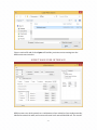
MPNET MAIN USER INTERFACE
MPNet treats a two-level network as a combination of two within level one-mode networks,
labelled as network A and B, and a two-mode meso-level network labelled as X. The overall
-7-
two-level network is labelled as network M in the MPNet output files. This means that you
may have two distinct node-sets, NA and NB, in which case A is the network (directed or
undirected) among the nodes in NA; B is the network (directed or undirected) among the
nodes in NB; and M is the bipartite network of ties between nodes in NA and nodes in NB.
The top left section of the user interface specifies the number of nodes involved in the levels
A and B , i.e. the number of nodes in NA and NB, respectively.
The top middle section specifies the functions the current session is performing, i.e. ERGM
simulation, ERGM estimation, test ERGM goodness of fit (GOF), or Bayesian estimation.
The tabbed panel on the right specifies function specific settings, such as setting for a
simulation section, including the number of simulation burn-ins, number of simulation
iterations and number of sample networks, etc.
The bottom left tabbed panels are interfaces designed for specifying network data involved
in an MPNet session.
The following section uses an example to demonstrate how to use MPNet to simulate onemode networks.
SIMULATING ONE-MODE NETWORKS
Simulating one-mode networks in MPNet will only involve network A, i.e. all data settings
are under the network A tab. The following settings or information are required for
simulations
Number of nodes: Type in the number of actors in the one mode network A.
Select “Simulation” radio button to perform model simulation.
-8-
Under the Model specification tabs, select network A, and click on the “Include” check box to
include the one-mode network A in this simulation session.
Network A can be directed or non-directed. Tick the “Directed” check box if we are
simulating a directed network. (Network A can also be treated as a fixed covariate in twolevel network models. Click the “Fixed” check box, if we want to treat network A as fixed
covariate.)
We can also simulate or estimate conditional models by ticking the “Fix density” check box
which will force the network density to be fixed, i.e. addition or deletion of network ties are
not possible under such condition. This option is useful in investigating properties of ERGM
parameters (and for estimation – below - when unconditional model convergence is hard to
reach.)
The starting density (between 0 and 1) is the density of a random network generated by
MPNet as the starting graph in the simulation. With fixed density, this will be the density of
all simulated graphs. If the density of the graph is not fixed, the value here will not affect the
longer term result of the simulation.
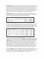
Click on the “Select parameters…” button to specify the model effects (parameters) and
graph statistics to be collected during the simulation. A parameter selection dialog will
show up with a list of implemented ERGM configurations for user selection.

The “include” column is a list of check boxes where if ticked, the corresponding
graph statistics will be included in the simulation.

The “Fixed” column is not implemented yet (which is designed for explore model
properties when certain effect is fixed). Please ignore for now.

The “λ” column provides the weighting parameter for the alternating statistics
introduced by Snijders et al. (2006). They are not in use for other statistics.

The “Value” column specifies parameter values for included effects. Here a Markov
model is specified with (EdgeA = -2; Star2A = 0.5; Star3A = -0.3; and TriangleA = 1.0).
We may include other graph statistics but leave the parameter values at 0 for MPNet
to generate the corresponding graph statistic distributions.
There are several buttons at the bottom of the parameter selection dialog:
-9-

“Clear All” will unselect all included configurations and set their parameter values to
0.

“Select All” will select all available parameters implemented under the current
dialog.

“Reset to 0s” will set all parameter values to 0.

“Exclude θ=0s” will unselect all statistics with parameter values as 0s.
The “Select All” and “Exclude θ=0” buttons become particularly useful for model GOF testing.
Click on “OK” to finalize the parameter selection.
- 10 -
Structural zero files: Part of a network can be treated as exogenous especially in the cases
of ERGM estimations where in some observed networks it makes empirical sense to fix part
of the network and estimate the structural features of the rest of the network given the
fixed part. To fix (or forbid the creation or deletion of) some of the network ties, one can
apply structural zero files in MPNet. For network of size n, the structural zero file contains
an n by n adjacency matrix of “1/0” indicators where 1 indicates the network tie is NOT
fixed, and 0 otherwise. Please check Appendix A for structural-zero file format.
Missing indicators: MPNet can estimate ERGM with missing network data following
Koskinen et al (2013). It is only used under Bayesian estimations. More detailed description
can be found in the Bayesian estimation section of this user manual.
Attribute/Dyadic covariates: Nodal attributes such as gender, age, performance, etc. can
be used as covariates in ERGMs to form social selection models (SSMs) (Robins et al, 2001).
Attributes or measurements on the tie variables or dyads (e.g. distance, strength) can be
treated as covariate under ERGMs. MPNet can handle binary, continuous, categorical nodal
attributes, as well as dyadic attributes for network ties as covariates for ERGMs.
Tick the corresponding types of attribute check boxes to enable attribute covariates.
Following the check boxes enter the number of attributes to be included in the simulation or
estimation. The covariate values are stored in Attribute files for binary, continuous and
categorical attribute: tab delimited text files where the first row of the file contains the
names of the attributes (e.g. gender, age, etc.), and each column contains the attribute
values in the same order as the nodes listed in the network matrices. The number of
columns must be the same as the number of attributes specified on the MPNet interface, or
MPNet will provide an error message. Attribute files for dyadic attribute are valued
adjacency matrices start with the attribute name; then stack one upon another depending
on the number of such attributes. See example attribute file formats in the Appendices.
Click on the “Browse…” button to specify the attribute file, and click on the “Select…” button
to select corresponding attribute configurations. The attribute names specified in the
attribute files will be loaded into the parameter selection dialog. The parameter selection
dialog follows the same format as the ERGM parameter selection dialog.
- 11 -
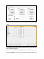
SIMULATION OPTIONS
The output files options enable us to pick sample graph matrices and sample degree
distributions as tab delimited files for further analysis using other software such as SPSS or
R.
Tick the “Sample networks” option will let the program generate each sample graph in
adjacency matrix format together with some graph statistics such as degree distributions
and global clustering coefficient, etc. The sample files are readable by the Pajek program for
the ease of visualizing the simulated samples. Be careful about the size of the sample
- 12 -
(‘Samples’) if you check this box because it can take a long time for the computer to write
out, for instance, 1000 files.
Tick the “Sample degree distribution” option to allow MPNet generating degree
distributions of simulated samples in tab delimited output together with the standard
deviations and skewness of the degree distributions.
The “Generate GCD” option will be implemented in a future release. It is only used in model
estimation or GOF testing with generalized Cook’s distances (GCDs) for each node as a
measure of how extreme or important each node is in contributing towards the network
structure (see Koskinen et al 2013 for more details)
Burn in is the first period of a simulation during which the simulation move towards the
desired graph distribution implied by the specified parameter values. Depending on the size
of the network and number of parameter values, the required burn-in can vary a lot. The
larger the network, or the more parameters, the longer burn-in is needed. Examination of
the output files can indicate whether the simulation has reached a consistent state and the
burn-in is sufficient. For instance, the number of edges in a stationary graph distribution
should vary consistently around a mean and not be consistently increasing or decreasing.
The Iterations box contains the number of proposed simulation updates after burn-in.
Samples expresses the number of graphs sampled from the simulation. Note that the
number of iterations between graph samples is calculated as the division between the
number of iterations and the number of samples to pick up.
Clicking on the Start button will start the simulation. Once the simulation finished, MPNet
will open the simulated graph statistics output file using your default text editor. You can
find all the output files in the session folder, i.e. where the MPNet session setting file is
allocated. More detailed descriptions of the output files are in the next section.
SIMULATION OUTPUT
MPNet will generate several output files upon finishing simulating the specified model.
Some of the output files are optional depending on the simulation settings described above.
Here is a list of possible output files and their content information. Note that depending on
the simulation settings, not all output file listed below would appear.
“MySession_Network_A_0.txt” is the initial or starting (Level A) graph for the simulation.
In a simulation session, it will be a random graph with the user specified density, i.e. the
starting density. It contains the adjacency matrix for the network and graph statistics such
as: density, mean degree, standard deviation and skewness of the degree distribution and
global clustering coefficient. For directed graphs, the output file will list statistics for in- and
out- degree distributions separately. This file can be read by Pajek for visualization. The
nodes will be plotted as blue squares.
- 13 -
“MySession_Network_A_1001000.txt” is the 1,001,000th simulated graph in the simulation.
The output file name depends on the number of interactions and samples, and it ends with
the last simulated network id. It has the same format as MySession_Network_A_0.txt.
“MySession_Network_B_0.txt” is the initial or starting (Level B) graph which follows the
same format as MySession_Network_A_0.txt. The nodes will be plotted as red circles in Pajek.
When only a unipartite graph distribution is simulated (i.e. the “Include” box is not ticked
for network B), this output will not appear.
“MySession_Network_X_0.txt” is the initial or starting meso-level two-mode graph which
list the two-mode network in edge-list format followed by some two-mode graph statistics.
Level A nodes will be plotted as blue squares, and level B nodes as red circles. When the
“Include” box is not ticked for network X, this output will not appear.
“MySession_Network_M_0.txt” contains the overall multilevel network in edge list format.
If the “Sample networks” option is selected under the Simulation/GOF tab, sample
network files following the same format as described above will be generated by MPNet.
“MySession.clu” is a Pajek cluster or partition file where the partitions are defined based
on the levels. Nodes in level A are in partition 0, and level B nodes are in partition 1. One
may use the cluster file to plot the meso or the overall two-level network in layers under
Pajek. Again, this requires the “Include” box to be ticked for network B.
“MySession_sim.txt” is the file opened by MPNet at the end of simulation which contains
the selected graph statistics. The statistics are listed in columns separated by tabs.
“MySession_spss.sps” is an SPSS script to plot the scatter-plot and histogram of the
simulated graph statistics using SPSS version 12.0 and above. It will read in the statistics in
MySession_sim.txt.
If the “Sample degree distributions” option is ticked under the Simulation/GOF tab, the
degrees of each node will be listed as tab delimited columns in the output files
“MySession_degreeA.txt”, “MySession_degreeB.txt” and “MySession_degreeX.txt”.
“MySession_model.txt” lists the parameter/statistic names, the lambda values, and the
parameter values used in the simulation.
SIMULATING TWO-MODE NETWORKS
To simulate two-mode networks, we need to specify the number of nodes in each modes (A
and B), e.g. to simulate a 16 by 12 bipartite network
- 14 -
The under “Model specifications”, click on “X (two-mode)” tab, and tick the Include check
box (make sure only network X is included. Inclusion of A or B networks will simulate the
corresponding one-mode networks together with the two-mode network.).
Most of the model specification settings are the same as in one mode networks (A or B),
except there is one more option as “No isolates”. Ticking such option in simulations or
estimations will ensure all nodes in the bipartite network to have a degree at least 1.
Similar to one-mode attribute files, the bipartite attribute covariate files contains attribute
values in tab delimited columns with attribute headers in the first row. However, as two
sets of nodes are involved, attribute values should be listed for A nodes first followed by B
nodes. For attribute that are only applicable to one set of nodes, 0s should be used for the
other set of nodes, and only relevant graph statistics or parameters should be selected
during simulation or estimation. For example, a 16 people (A) by 12 club (B) bipartite graph
with the gender as binary attribute for people, the binary attribute file should start with
“gender” as header followed by a column of 28 attribute values where the first 16 is defined
by the gender of people, the rest 12 should be listed as 0s.
Other simulation settings and output files are very similar to the setting and outputs in
simulations for one-mode networks as described in the previous section.
SIMULATING TWO LEVEL NETWORKS
Simulating two-level networks will require the number of nodes in both levels (A and B),
and the inclusion of all three networks (A, B and X) by ticking the “Include” check boxes
under each of the tabs (A, B and X) under model specifications. The within- (A and B) and
meso-level (X) model parameters/statistics can be selected under the corresponding tabs.
The statistics involving network ties from different networks can be selected under the “A X
B” tab:
- 15 -
Click on the “Structure” buttons to open the corresponding parameter selection dialogs with
configurations representing interactions among ties across the levels. Using “A and X” as an
example
The dialog shares the same format as parameter selection dialogues for one or two-mode
network simulations/estimations.
For multilevel social selection models, MPNet require attribute files before the user can
select attribute parameters. The attribute file format follows the format as described in the
section for simulating two-mode networks, i.e. tab delimited columns with headers in the
- 16 -
first row, and attribute values from nodes of type A followed by nodes of type B; using 0 as
values for attributes that do not apply to either types of nodes.
Other simulation settings and simulation output files are similar to simulations for one- or
two-mode networks as described in previous sections.
ESTIMATION
Estimating ERGM parameters under MPNet require the user to specify the network data to
be modelled, the ERGM specification and some estimation options. MPNet implements
Markov Chain Monte Carlo Maximum Likelihood estimation algorithm as proposed by
Snijders (2002) based on the Robbins-Monro procedure (1951). MPNet can model one- (A)
or two-mode (X) networks, a combination of one and two-mode networks (A and X), and
two-level networks (A, B and X).
To estimate a model, start MPNet and provide a session name for a new session. Select the
“Estimation” radio button. You may also continue from a previous session. Note that in
contrast to PNet, you may change data set and specifications in an active or saved session.
Upon selecting the “Estimation” option, the “Network File” text box is enabled under the
“Model specification” tabs for user to specify the network data. Click on the “Browse…”
button to specify the network file which has the format of a raw adjacency matrix. The
number of rows and columns of the matrix must be the same as the number of nodes
specified. Please refer to the Appendices for an example network file.
ESTIMATING ERGMS FOR ONE-MODE NETWORKS
To estimate models for one-mode networks, only inclusion of network A is required. Tick
the “Directed” option if the network is directed. For estimations of models conditioning on
the density of the network, tick the “Fix density” option. Click on “Select parameters…” to
open the parameter selection dialog.
- 17 -
Select the effects to be included in the model under estimation by ticking the check boxes
under the “Include” column. The “Value” column contains the starting parameter values. If
we leave all parameters at 0s, MPNet will start estimation with an Edge or Arc parameter
calculated based on the density of the network. Note that if we are estimating a model
conditioning on the density of the network, please do not select Edge or Arc parameter. The
model specificantion implemented in MPNet follows the Markov (Frank and Strauss, 1986)
and the social circuit (Snijders et al, 2006; Robins et al,2009) assumptions. Some higher
order configurations are also implemented based on Pattision and Snijders (2013). Please
refer to the Appendices for a list of implemented model configurations.
ESTIMATING ERGMS FOR TWO MODE NETWORKS
To estimate ERGMs for two mode networks, we need to specify the number of nodes in set A
and set B. Then, only include network X under the Model specification tabs. The network file
is a n by m rectangular matrix if we have n nodes in set A and m nodes in set B. Possible
conditional ERGMs including fixing the density of the network (the “Fix density” option), or
enforce nodes to have degrees at least 1 (the “No isolates” option). Click on the “Select
parameters…” button to open the parameter selection dialog. The implemented two-mode
configurations follows the model specifications proposed in (Wang et al, 2009; 2013) as
shown in the Appendices.
- 18 -
ESTIMATING ERGMS FOR COMBINED ONE- AND TWO- MODE NETWORKS
Estimating ERGMs for a combined one- and two-model networks require inclusion of
network A, X and their corresponding network files. The within one- or two-mode network
effects are the same as in separate models for network A or B. The interaction effects
between network A and X can be selected under the “A X B” tab by ticking the check box
next to the “Structure” button under “A and X”. The interaction configurations can be
selected by click on the “Structure” button, and they follow the specifications proposed in
Wang et al (2013). See the appendices for a list of configurations.
ESTIMATING ERGMS FOR TWO-LEVEL NETWORKS
ERGMs for two-level networks require network files for all networks A, B and X. The
possible within- and meso-level model configurations follow the same specifications as in
models for individual one- or two-mode networks. The interaction effects among the
networks A, B and X can be selected by the “Structure” buttons for the corresponding
interactions under the “A X B” tab. The implemented model configurations follow Wang et al
(2013), and they are listed in the Appendices.
ESTIMATING ERGMS WITH NODAL ATTRIBUTES AS COVARIATES
- 19 -
MPNet can model network structures with nodal attributes as covariates. The attribute file
inputs are the same as described in the Simulation section. Note that separate attribute files
are required for each of the networks under the Model specification tabs. The attribute file
format for the interactions among networks A, B and X are the same as attribute file for
bipartite network (X), i.e. columns of attribute values starting with attribute names, then
attribute values for A nodes then B nodes, with 0s represent attribute values that do not
apply to either set of nodes.
ESTIMATING CONDITIONAL ERGMS
Besides using nodal attributes as covariates, we may also treat one or more of the three
networks involved in the two-level network as fixed and exogenous. The research question
is then about how one given network affects the structures of the other networks. For
example, how club membership (fixed two-mode network X) may affect friendship (onemode network A), or vice versa. Snijders and Van Duijn (2002) has a detailed discussions on
conditional estimations for ERGMs with covariates. To fix one or more networks as
covariates, tick the “Fixed” option under the tabs for the corresponding networks; and make
sure no parameters are selected for fixed networks.
OPTIONS FOR THE ESTIMATION ALGORITHM:
The MCMCMLE algorithm has several customizable settings or options modifying which
may help model convergence.
- 20 -
Subphases: Each sub-phase refines the parameter values, but more sub-phases do not
guarantee convergence. The default value is 5. If a good set of starting parameter values is
available, a smaller number of sub-phases may help reduce time required for the estimation.
Gaining Factor is a multiplier that affects the sizes of parameter updates. It is halved after
each sub-phase to refine the parameter values as the model converges. The default a-value
is 0.01. Smaller a-values may be used, if a good set of starting parameter values is available.
Multiplication Factor is a multiplier that determines the number of simulation iterations
between network samples during estimations (other factors including the size and the
density of the network). The larger the multiplication factor, the greater the distances
between network samples, and hence the smaller the auto-correlations between samples
which may yield a more reliable model. Networks with greater number of nodes may
require greater multiplication factors to achieve model convergence. However, greater
multiplication factor will also result in longer estimation time. The default value is 10 but
for directed networks and larger networks a larger multiplication factor is generally needed.
It is rare that estimation requires a larger multiplication factor than 100. If the SACF (see
OUTPUT below) is greater than 0.4 you will need to increase the multiplication factor.
Iterations in phase 3: In phase 3, MPNet simulates network graphs using estimated
parameters obtained from phase 2, and produces t-statistics based on comparisons
between the simulated graph distribution and the observed graph statistics. The default
value is 500 samples. Note that the number of simulation updates between samples is the
same as in the estimation which is determined by the network size, network density, and
the multiplication factor.
Max. estimation runs: As default, the program will perform one estimation and stop.
Multiple estimations runs in sequence can be performed such that each new run uses the
parameter values obtained from the end of the previous run. An improved parameter
estimate may be obtained as the new estimation may start with a set of parameter values
closer to convergence. MPNet will stop and ignore the subsequent estimation runs as soon
as the model is converged; otherwise the maximum number of estimation runs will be
performed.
Do GOF at convergence: PNet can perform a goodness of fit (GOF) examination once the
model under estimation has converged. The GOF output file will be located in the session
folder. See detailed description of the GOF test in the next section.
Click on Start button to start the estimation. Upon completion of the estimation, MPNet will
show you whether the model has converged or not, and open the estimated model with the
default text editor.
After first estimation run, the Update button will be enabled. It is used when you want to
start the next estimation run with previous estimated parameters so that you may start the
new estimation from a better set of parameter values.
ESTIMATION OUTPUT
- 21 -
For a MPNet estimation session with session name “MySession”, MPNet will generate the
following output:
“MySession_Network_A_0.txt”, “MySession_Network_B_0.txt”,
“MySession_Network_X_0.txt”, and “MySession_Network_M_0.txt” are the networks that
have been modelled in adjacency matrix format for networks A and B, and edge list format
for networks X and the overall two-level network M. The content of the files are the same as
output from a simulation session as described previously.
“MySession__model.txt” contains the model specification during the estimation session,
and the starting parameter values.
“MySession_update.txt” contains the model specification during the estimation session,
and the most recent parameter estimates. MPNet uses this file for updating parameter
values when the Update button is clicked.
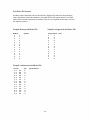
“MySession_est.txt” contains all parameter estimates throughout the entire estimation
session, i.e. any estimation runs under this session name will be appended towards the
bottom of this file. The most recent estimates are listed at the end of the file. The
“Estimation results” section of the output lists the effect names, parameter estimates,
estimated standard errors, t-ratio for convergence test, and sample autocorrelation
functions (SACF) for a reliability check. They are listed in tab delimited columns which you
may copy and paste into table format (e g. In Excel). Here is an example output:
Effects
EdgeA
ASA
ATA
A2PA
Lambda Parameter Stderr
t-ratio
SACF
2
-3.3993
1.421
-0.092
0.065 *
2
1.028
0.505
-0.078
0.064 *
2
-0.06
0.249
-0.069
0.077
2
-0.2094
0.251
-0.071
0.061
When all t-ratios in the estimated model have absolute values smaller than 0.1, we consider
the model is well converged. SACFs smaller than 0.4 indicates there are sufficient distances
between simulated samples during the estimation, hence the model is more reliable. We
consider the absolute value of a parameter estimate greater than twice the size of the
estimated standard errors as significant, and they are indicated by “*”.
The variance covariance matrix of the estimated parameters is listed at the end of the
estimation output. This may be useful for Bayesian estimations described below.
GOODNESS OF FIT
Once a converged ERGM is obtained, the model goodness of fit (GOF) can be tested by
comparing simulated graph statistics of the estimated model against the network that has
been modelled. The graph statistics are not limited to the ones that are already included in
- 22 -
the model, but also a greater range of configurations representing the network structure.
Click on the GOF radio button to specify a model GOF session.
GOODNESS OF FIT SETUP
Most settings for Goodness of Fit are the same as in Simulation, except the observed
network and parameter values are required. The observed network file can be specified the
same as in Estimation. The parameter values can be typed under the corresponding model
parameter selection dialog; or by using the “Update” button if the GOF session is for the
most recently converged model under Estimation.
During model parameter selection, click on the “Select All” button will include all
implemented statistics in the GOF simulation.
Other GOF settings are the same as in Simulations. At the end of the GOF simulation, MPNet
will calculate t-ratios for all included graph statistics. For configurations that are already
included in the model, t-ratios smaller than 0.1 in absolute value reconfirm the model is
converged (if there is a discrepancy between the estimation convergence statistics and the
GOF t-ratios, you may have to increase the ratio of the number of iterations to the number of
- 23 -
samples (See more detailed discussions in Koskinen and Snijders (2012) Chapter 12 of the
book on ERGMs). For other statistics, t-ratios smaller than 2.0 in absolute values suggest
adequate fit to that particular graph feature. T-ratios greater than 2.0 standard deviation
units from the mean indicate poor fit to the data on that particular graph feature.
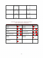
GOODNESS OF FIT OUTPUT
Besides the same sets of output files as in Simulation session, MPNet will generate a GOF
result file namely “MySession_gof.txt”. It contains a tab delimited table where the first
column lists the configurations included in the GOF simulation; the second column contains
the counts of the configurations in the observed network; the third column contains the
means of the simulated graph statistic distribution; the third column has the standard
deviations; the fourth column shows the t-ratios; and the last column shows “#” signs for tratios that are greater than 2.0 in absolute values indicating poor fit to the corresponding
statistics. Below is an example output for a GOF test of a one-mode network A.
Besides the user selected configurations, MPNet also includes some global network
measurements as part of the output, including the standard deviation and skewness of the
degree distributions and the global clustering coefficient. The Mahalanobis distance shown
at the end of the file is an overall heuristic measure of model GOF, taking into account the
covariance of the included statistics. Smaller Mahalanobis distances indicate better fit to the
dat. (Wang et al 2009). Mahalanobis distance should not be tested with standard chisquared statistics: in this context, it is an indicative measure. If two models have the same
configurations in the GOF output, then the one with the lower Mahalanobis distance is a
better fit.
Configuration
Observed Mean
StdDev t-ratio
EdgeA
22
22.39
3.98
-0.09
Star2A
71
65.84
24.58
0.21
Star3A
62
59.14
36.77
0.07
Star4A
30
36.16
35.31
-0.17
Star5A
8
15.68
24.14
-0.31
TriangleA
7
5.33
3.65
0.45
Cycle4A
16
10.78
9.47
0.55
IsolatesA
2
0.32
0.59
2.84 #
IsolateEdgesA
0
0.02
0.15
-0.15
ASA
46.56
43.62
12.82
0.22
ATA
17.75
13.64
8.13
0.50
A2PA
57.12
56.06
17.34
0.06
AETA
33.62
24.39
19.15
0.48
stddev_degreeA
2.51
2.22
0.33
0.87
skew_degreeA
1.06
1.30
0.15
-1.60
clusteringA
0.29
0.22
0.09
0.77
Mahalanobis distance = 193
- 24 -
BAYESIAN ESTIMATION
MPNet implements a version of the Bayesian estimation algorithm proposed by Camio and
Friel (2009) as specified in Koskinen et al (2013). Instead of obtaining the point estimates
as in MCMCMLE, the Bayesian estimation generates the posterior distributions of the model
parameters. In lieu of MLEs and standard errors, point estimates and measures of
uncertainty are calculated as averages and standards errors of this distribution respectively.
The approximations of Phase 3 are thus not necessary. However, as the posterior is
generated using an iterative MCMC algorithm it is important to assess ‘mixing’, i.e., how well
the algorithm samples from the posterior..
Select “Bayesian estimation” from the main user interface, the Bayesian estimation options
will be enabled. The same as in Estimation, network data input file and model parameter
selections can be specified under the “Model specification” tabs. The setting options for
Bayesian estimations are different from Estimations as shown on the right side of the user
interface.
BAYESIAN ESTIMATION SETTINGS
- 25 -
Parameter burn-in: similar to burn-in for simulations, the starting parameters may be
considered extreme from the posterior parameter distribution. The burn-in will discard the
specified number of parameter updates at the beginning of the estimation.
Proposal scaling: similar to a-values in maximum likelihood estimations (MLEs), the
proposal scaling (or ‘step-size constant’; Tierney, 1994) is a multiplier for the sizes of
parameter updates. Greater scaling will cover greater range for parameter proposals;
however, greater scaling may also reduce the number of accepted parameter proposals as
part of the posterior. The proposal distribution in the Metropolis algorithm is Np(,S), where
 is the current value, S=c/(1+p) , and  is some estimate of the variance-covariance
matrix of the posterior distribution. In this expression c is the ‘proposal scaling’.
Multiplication factor: is the same as in MLEs, and determines the number of iterations to
be simulated in order to generate a network given a proposed parameter. The
multiplication factor generally speaking should be about three times as large as for the nonBayesian algorithm.
MCMC Sample size: is the number of parameter proposals. If all parameter proposals are
accepted, the posterior will contain this number of parameter sets. (Note that achieving
100% acceptance of proposed parameter values are not the goal of the estimation.
Acceptance of all proposals suggesting the resulting posterior may only cover part of the
actual posterior, and a greater proposal scaling may be required.) The larger the MCMC
Sample size, the better the precision of the posterior mean and standard deviation (given a
fixed acceptance rate).
Max. estimation runs, Do GOF at convergence and Generate GCD at convergence: they
are not applicable in Bayesian estimations.
Maximum lag (SACF): determines the largest lag (distance) for which the sample
autocorrelation function for the estimated posterior is. In order for the effective sample
size (ESS) to be reliable, the autocorrelation at the Maximum lag has to be sufficiently close
to zero (as a rule of thumb, smaller than 0.05 in absolute value). The lag at which the SACF
value is approximately zero is gives the number of parameter draws you need to discard inbetween every successive parameter value that you base your posterior inference on. For
example, if the SACF at lag 100 is approximately zero, then you need an MCNC sample size
of 100,000 to get 1000 independent draws from the posterior distribution. If the SACF at lag
100 is greater than, say, 0.4 you need to modify the parameter proposals by increasing the
‘proposal scaling’.
There are several possible matrices we may apply to Bayesian estimation which is used for
determining the ‘direction’ of parameter updates. There are four options approximating ,
which is used to set the proposal variance-covariance matrix through S=c/(1+p) .
Scaled identity matrix: An identity matrix that implies no preferred direction of updates.
The directions of updates are solely based on the difference statistics between the observed
graph and the simulated samples.
Combined simulation: only applicable for Bayesian estimations with missing data as in
Koskinen et al (2013). See more detailed instructions in the next section.
- 26 -
Nonconditional simulation: the differences between the observed graph and the
simulated samples are refined by a covariance matrix generated based on a simulation with
the starting parameters. (This is an analogous procedure to the one employed in Phase 1 of
the non-Bayesian estimation)
Covariance file: A user defined covariance matrices of the parameters are used to refine
the direction of parameter updates. The covariance file is a p by p matrix if there are p
parameters in the model. Such covariance file may be obtained based on previous
estimations of the same model. MPNet generates such files at the end of estimations with
file name e.g. “MySession_varcov.txt”. If this estimate of  is close to the true posterior
variance-covariance matrix, the proposal scaling c should be in the range of 0.5 to 4.
BAYESIAN ESTIMATION OUTPUTS
Bayesian estimation summarize the estimation results in two file
“MySession_posterior_bayesian.txt” contains the estimated posterior. It has p tab
delimited columns for models with p parameters; each column contains the accepted
parameter values in the posterior with parameter names on the first row. The posterior can
be plotted by software such as R, Excel, etc. Plotting the parameter draws across iterations
gives a quick indication of whether the algorithm performs well. If there is ‘drift’, better
initial values and a longer burn-in may be needed. If the parameters move slowly (there is
great autocorrelation) between different values, a larger proposal scaling is needed.
“MySession_est_bayesian.txt”: As shown in the example below, the output summarizes the
parameter posterior distributions in terms of means and standard deviation, followed by
the covariance matrix of the parameters. Since there is no convergence test for Bayesian
estimation, the reliability of the generated posterior is indicated by the sample
autocorrelation functions (SACFs) for different lags up to the user defined maximum lag.
The maximum lag should be set to the lag for which SACF is approximately zero, then the
effective sample size (ESS) can be trusted (the calculation of ESS here is based only on lags
up to and including the max lag). Increasing the proposal scaling will decrease the SACF. If
you use ‘scaled identity’ and the SACF differs a lot between parameters, change to option
‘Covariance file’.
Acceptance rate: 0.38
Estimation results
Effects Lambda
PostMean Stddev
EdgeA
2
-2.513
1.173 *
ASA
2
0.4911
0.492
ATA
2
0.0097
0.25
A2PA
2
-0.0568
0.317
Covariance matrix
1.3752
-0.3789
0.0932
-0.1083
- 27 -
-0.3789
0.0932
-0.1083
SACF
Effect
EdgeA
ASA
ATA
A2PA
0.2423
-0.0467
-0.0736
-0.0467
0.0624
-0.0139
-0.0736
-0.0139
0.1004
10
0.993
0.976
0.888
0.953
30
0.98
0.935
0.711
0.882
50
0.969
0.895
0.572
0.824
70
0.96
0.86
0.466
0.779
90 ESS(100)
0.951
51
0.825
55
0.378
82
0.73
60
BAYESIAN ESTIMATIONS WITH MISSING NETWORK DATA
Following Koskinen et al (2013), MPNet implements Bayesian estimations with missing
network ties. The assumption is that we have the information about which network ties are
missing, and the missing ties follow the same social processes as the observed part of the
network. The current implementation of MPNet can only estimate models for one-mode
networks (A). Future release will extend the method to two-mode and two-level networks.
The estimation settings mostly follows settings under Bayesian estimation, except it
requires a missing indicator file, and the use of the “Combined simulation” estimation
option.
The missing indicator file has the same format as the network file, i.e. an adjacency matrix of
1s and 0s, where 1s indicate ties that are part of the missing data and 0s indicate nonmissing ties. The missing indicator file can be specified under Model specification tabs by
ticking the “Missing indicators” check box, and clicking on the “Browse…” button.
It is advisable to start estimation with ‘Scaled identity matrix’ but if a short estimation
round yields reasonable preliminary estimates, better performance of the algorithm may be
had from using ‘Combined simulation’ in the options under Bayesian estimation.
- 28 -
The output of Bayesian missing data estimation is the same as in Bayesian estimations
without missing data.
- 29 -
REFERENCES
Caimo, A., & Friel, N. (2011). Bayesian inference for exponential random graph models. Social
Networks, 33(1), 41-55.
Daraganova, G., Robins, G. Auto-logistic actor-attribute models. (2013) In Lusher, D., Koskinen,
J., & Robins, G. (eds). Exponential Random Graph Models for Social Networks: Theories,
Methods and Applications. New York: Cambridge University Press.
Erdős, P., & Rényi, A. (1976). On the evolution of random graphs. Selected Papers of Alfréd
Rényi, vol, 2, 482-525.
Frank, O., & Strauss, D. (1986). Markov graphs. Journal of the American Statistical
association, 81(395), 832-842.
Handcock, M. S., Robins, G., Snijders, T. A., Moody, J., & Besag, J. (2003).Assessing
degeneracy in statistical models of social networks (Vol. 39). Working paper.
Handcock, M. S., Hunter, D., Butts, C. T., Goodreau, S. M., & Morris, M. (2003). statnet: An R
package for the Statistical Modeling of Social Networks.Web page http://www. csde. washington.
edu/statnet.
Holland, P. W., & Leinhardt, S. (1981). An exponential family of probability distributions for
directed graphs. Journal of the american Statistical association,76(373), 33-50.
Hunter, D. R. (2007). Curved exponential family models for social networks.Social
networks, 29(2), 216-230.
Koskinen, J. H., Robins, G. L., & Pattison, P. E. (2010). Analysing exponential random graph (pstar) models with missing data using Bayesian data augmentation. Statistical Methodology, 7(3),
366-384.
Koskinen, J. H., Robins, G. L., Wang, P., and Pattison, P. E. (2013). Bayesian analysis for
partially observed network data, missing ties, attributes and actors. Social Networks, vol. 35(4),
514-527.
Koskinen, J. H., & Snijders, T. A. (2012) Simulation, Estimation, and Goodness of Fit. In Lusher,
D., Koskinen, J., & Robins, G. (Eds.). Exponential Random Graph Models for Social Networks:
Theory, Methods, and Applications. Cambridge University Press.
Lusher, D., Koskinen, J., & Robins, G. (Eds.). (2012). Exponential Random Graph Models for
Social Networks: Theory, Methods, and Applications. Cambridge University Press.
Pattison, P., & Robins, G. (2002). Neighborhood–based models for social networks. Sociological
Methodology, 32(1), 301-337.
Pattison, P., & Robins, G. (2004). Building models for social space: neighourhood-based models
for social networks and affiliation structures.Mathématiques et sciences humaines. Mathematics
and social sciences, (168).
Pattison, P., & Wasserman, S. (1999). Logit models and logistic regressions for social networks:
II. Multivariate relations. British Journal of Mathematical and Statistical Psychology, 52(2), 169193.
- 30 -
Robbins, H., & Monro, S. (1951). A stochastic approximation method. The annals of mathematical
statistics, 400-407.
Robins, G., Pattison, P., Kalish, Y., & Lusher, D. (2007). An introduction to exponential random
graph ( p*) models for social networks. Social networks, 29(2), 173-191.
Robins, G., Snijders, T., Wang, P., Handcock, M., & Pattison, P. (2007). Recent developments in
exponential random graph (< i> p</i>*) models for social networks. Social networks, 29(2), 192215.
Robins, G., Elliott, P., & Pattison, P. (2001). Network models for social selection
processes. Social Networks, 23(1), 1-30.
Robins, G.L., Pattison, P, & Elliott, P. (2001b). Network models for social influence processes.
Psychometrika, 66, 161-190.
Robins, G., Pattison, P., & Wang, P. (2009). Closure, connectivity and degree distributions:
exponential random graph (p*) models for directed social networks. Social Networks, 31, 105117.
Snijders, T. A. (2002). Markov chain Monte Carlo estimation of exponential random graph
models. Journal of Social Structure, 3(2), 1-40.
Snijders, T. A., Pattison, P. E., Robins, G. L., & Handcock, M. S. (2006). New specifications for
exponential random graph models. Sociological methodology,36(1), 99-153.
Snijders, T. A., Van de Bunt, G. G., & Steglich, C. E. (2010). Introduction to stochastic actorbased models for network dynamics. Social networks, 32(1), 44-60.
Tierney, L. (1994) Markov Chains for Exploring Posterior Distributions. The Annals of Statistics 22
(4), 1701--1728.
Wang, P., Robins, G., Pattison, P., & Lazega, E. (2013). Exponential random graph models for
multilevel networks. Social Networks 35(1), 96-115.
Wang, P., Robins, G., Pattison, P., & Lazega, E. (under review). Social selection models for
multilevel networks.
Wang, P., Sharpe, K., Robins, G. L., & Pattison, P. E. (2009). Exponential random graph (p*)
models for affiliation networks. Social Networks, 31(1), 12-25.
Wasserman, S. and Pattison, P. (1996). Logit models and logistic regressions for social networks:
I. an introduction to Markov graphs and p*. Psychometrika, 61(3):401–425.
- 31 -
APPENDIX A – SAMPLE FILES
SAMPLE INPUT FILES
Sample network file:
……
0 0 8 0 4
0 0 0 9 0
Strength
0 1 5 0 7
0 0 0 0 0
……
……
0 3 0 0 0
0 6 0 0 0
0 0 7 0 0
Network files contain the observed
network in the adjacency matrix format.
0
0
0
0
0
0
0
0
0
0
0
0
0
0
0
0
0
0
0
0
0
0
0
0
0
0
0
0
0
0
0
0
0
1
0
0
0
0
0
0
0
0
0
0
0
0
1
0
0
0
0
0
0
0
0
0
0
0
1
1
0
1
1
1
0
0
0
0
0
0
0
0
0
1
0
0
0
0
0
0
0
0
0
1
0
0
0
0
0
0
0
0
0
0
0
0
0
0
0
0
0
0
0
1
0
0
0
1
0
0
1
0
0
0
0
0
0
0
0
1
0
1
0
1
0
0
0
0
0
0
0
0
0
1
0
0
0
0
0
1
0
0
1
0
0
0
0
1
0
1
0
0
0
0
0
0
1
1
0
0
0
0
0
0
0
0
0
0
0
0
0
0
0
0
0
0
0
0
0
0
0
0
0
0
0
0
0
0
0
0
1
0
1
0
0
0
3 0 1 0 0 0 0 0 0
1 4 0 2 1 0 0 0 0
0 4 0 0 5 0 0 9 0
0 0 0 3 0 0 0 0 0
0 0 5 1 0 0 0 0 0
0 0 1 0 0 0 7 0 0
1 0 0 7 1 0 0 8 0
Sample structural zero file:
The file contains a binary matrix where ‘1’
indicates changeable ties, and ‘0’ indicates
fixed ties. Applying this structural zero
file example will fix all the tie variables
related to node 2 and 5. Ties between
node 1 and 13, node 1 and 14, are also
fixed.
Sample dyadic attribute file
Dyadic attribute files contain the values of
network ties as covariate in the adjacency
matrix format with headers as attribute
names. Multiple dyadic attributes are
listed in the same file each with separate
headers.
0
0
1
1
0
1
1
1
1
1
1
1
1
1
Note: Examples here omitted some values
in the matrices.
Distance
0 1 5 0 7 0 4 0 0 5 0 0 9 0
0 0 0 0 0 0 0 0 0 0 0 0 0 0
……
- 32 -
0
0
0
0
0
0
0
0
0
0
0
0
0
0
1
0
0
1
0
1
1
1
1
1
1
1
1
1
1
0
1
0
0
1
1
1
1
1
1
1
1
1
0
0
0
0
0
0
0
0
0
0
0
0
0
0
1
0
1
1
0
0
1
1
1
1
1
1
1
1
1
0
1
1
0
1
0
1
1
1
1
1
1
1
1
0
1
1
0
1
1
0
1
1
1
1
1
1
1
0
1
1
0
1
1
1
0
1
1
1
1
1
1
0
1
1
0
1
1
1
1
0
1
1
1
1
1
0
1
1
0
1
1
1
1
1
0
1
1
1
1
0
1
1
0
1
1
1
1
1
1
0
1
1
0
0
1
1
0
1
1
1
1
1
1
1
0
1
0
0
1
1
0
1
1
1
1
1
1
1
1
0
Attribute file format
Attribute names should be listed in the first line, delimited by tabs. Note that attribute
names should not start with numbers to meet the SPSS script requirements for variable
names. Each column represents an attribute. Each row corresponds to the same row as in
the adjacency matrix
Sample binary attribute file:
Member
1
1
0
1
1
0
1
0
1
1
0
0
0
1
Sample categorical attribute file:
gender
Department club
1
1
3
2
2
3
3
2
1
3
2
1
1
2
2
3
3
1
3
3
2
2
3
2
1
1
1
2
1
1
1
0
1
0
0
0
1
0
1
0
1
0
Sample continuous attribute file:
Income
1.0
1.1
1.1
0.5
0.3
1.1
1.5
0.2
0.1
0.2
1.0
0.2
0.1
0.5
23
34
42
23
24
19
38
49
58
47
24
36
19
20
age
2
6
5
4
1
1
2
1
1
2
3
2
4
3
performance
- 33 -
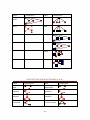
APPENDIX B – MODEL CONFIGURATIONS
NON-DIRECTED ONE-MODE
NETWORKS (A & B)
Label
EdgeA
EdgeB
Star2A
Star2B
Configuration
BIPARTITE NETWORKS (X)
Label
XEdge
XStar2A
Star3A
Star3B
XStar2B
Star4A
Star4B
XStar3A
Star5A
Star5B
XStar3B
TriangleA
TriangleB
X3Path
Cycle4A
Cycle4B
X4Cycle
IsolatesA
IsolatesB
XECA
IsolateEdgesA
IsolateEdgesB
XECB
ASA
ASA2
ASB
ASB2
ATA
ATB
IsolatesXA
…
…
IsolatesXB
- 34 -
Configuration
Label
A2PA
A2PB
Configuration
…
AETA
Label
XASA
Configuration
…
XASB
…
XACA
…
XACB
…
…
XAECA
…
XAECB
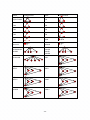
DIRECTED ONE-MODE NETWORKS (A & B)
Label
ArcA
ArcB
In2StarA
In2StarB
Configuration
Label
ReciprocityA
ReciprocityB
Out2StarA
Out2StarB
In3StarA
In3StarB
Out3StarA
Out3StarB
TwoPathA
TwoPathB
Transitive-TriadA
Transitive-TriadB
- 35 -
Configuration
Label
Cyclic-TriadA
Cyclic-TriadB
Configuration
Label
T1A
T1B
T2A
T2B
T3A
T3B
T4A
T4B
T5A
T5B
T6A
T6B
T7A
T7B
T8A
T8B
SinkA
SinkB
SourceA
SourceB
IsolateA
IsolateB
AinSA
AinSA2AinSB
AinSB2
AoutSA
AoutSA2
AoutSB
AoutSB2
ATA-T
ATB-T
AinAoutSA
AinAoutSB
ATA-C
ATB-C
ATA-U
ATB-U
A2PA-D
A2PB-D
…
…
…
…
…
…
ATA-D
ATB-D
A2PA-T
A2PB-T
A2PA-U
A2PB-U
- 36 -
Configuration
…
…
…
…
…
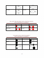
NON-DIRECTED ONE- AND TWO-MODE INTERACTIONS (A & X, OR B & X)
Label
Star2AX
Configuration
Label
Star2BX
StarAB1X
…
StarAA1X
Configuration
…
StarAX1A
StarAX1B
…
…
…
StarAXAB
…
StarAXAA
TriangleXBX
L3XAX
L3XBX
ATXAX
ATXBX
…
TriangleXAX
…
EXTA
EXTB
- 37 -
DIRECTED ONE- AND TWO-MODE INTERACTIONS (A & X, OR B & X)
Label
In2StarAX
Configuration
Label
In2StarBX
Out2StarAX
Out2StarBX
AXS1Ain
AXS1Bin
…
…
AXS1Aout
Configuration
AXS1Bout
…
…
ABinS1X
…
AAinS1X
…
ABoutS1X
…
TXAXarc
TXBXarc
TXAXreciprocity
TXBXreciprocity
- 38 -
…
AAoutS1X
ATXBXarc
…
ATXAXarc
…
ATXBXreciprocity
…
ATXAXreciprocity
…
L3XAX
L3XBX
L3XAXreciprocity
L3XBXreciprocity
NON-DIRECTED CROSS-LEVEL INTERACTIONS (A, B & X)
Label
L3AXB
ASAXASB
Configuration
Label
C4AXB
AC4AXB
- 39 -
Configuration
DIRECTED CROSS-LEVEL INTERACTIONS (A, B & X)
Label
L3AXBin
Configuration
Label
L3AXBout
L3AXBpath
L3BXApath
C4AXBentrainment
C4AXBexchange
C4AXBexchangeAreciprocity
C4AXBexchangeBreciprocity
C4AXBreciprocity
C4AXBexchangeBreciprocity
AinASXAinBS
AoutASXAoutBS
AinASXAoutBS
AoutASXAinBS
- 40 -
Configuration
NON-DIRECTED ONE-MODE SOCIAL SELECTION MODELS
WITH BINARY ATTRIBUTES
Label
ActivityA
ActivityB
TwoPath100A
TwoPath100B
Configuration
Label
InteractionA
InteractionB
TwoPath010A
TwoPath010B
TwoPath110A
TwoPath110B
TwoPath101A
TwoPath101B
TwoPath111A
TwoPath111B
Triangle1A
Triangle1B
Triangle2A
Triangle2B
Triangle3A
Triangle3B
Configuration
TWO-MODE SOCIAL SELECTION MODELS
WITH BINARY ATTRIBUTES
Label
XEdgeA
Configuration
Label
XEdgeB
X2StarA010
X2StarB010
X2StarA100
X2StarB100
X2StarA101
X2StarB101
- 41 -
Configuration
X4CycleA1
X4CycleB1
X4CycleA2
X4CycleB2
NON-DIRECTED ONE-MODE SOCIAL SELECTION MODELS
WITH CONTINUOUS ATTRIBUTES
Label
ActivityA
ActivityB
Configuration Label
SumA
SumB
DifferenceA
DifferenceB
Configuration
ProductA
ProductB
TWO-MODE SOCIAL SELECTION MODELS
WITH CONTINUOUS ATTRIBUTES
Label
XEdgeA
Configuration
Label
XEdgeB
X2StarA
X2StarB
X2StarASum
X2StarBSum
- 42 -
Configuration
X2StarADifference
X2StarBDifference
X4CycleASum
X4CycleBSum
X4CycleADifference
X4CycleBDifference
XEdgeABSum
XEdgeABDifference
ONE- AND TWO-MODE SOCIAL SELECTION MODELS
WITH CATEGORICAL ATTRIBUTES
Label
MatchA
MatchB
MismatchA
MismatchB
X2StarAMatch
Configuration
Label
MismatchA
MismatchB
X2StarBMatch
X2StarAMismatch
X2StarBMismatch
X4CycleAMatch
X4CycleBMatch
- 43 -
Configuration
X4CycleAMismatch
X4CycleBMismatch
XEdgeMatchAB
XEdgeMismatchAB
DIRECTED ONE-MODE SOCIAL SELECTION MODELS
WITH BINARY ATTRIBUTES
Label
SenderA
SenderB
InteractionA
InteractionB
InteractionReciprocityA
InteractionReciprocityB
Out2Star010A
Out2Star010B
Configuration Label
ReceiverA
ReceiverB
ActivityReciprocityA
ActivityReciprocityB
In2Star010A
In2Star010B
Configuration
Mix2Star010A
Mixed2Star010B
DIRECTED CROSS LEVEL SOCIAL SELECTION MODELS
WITH BINARY ATTRIBUTES
Label
L3AXBSenderAB
L3ASXBRpath
Configuration Label
L3AXBReceiverAB
L3ARXBSpath
- 44 -
Configuration
C4AXBentrainmentA
C4AXBentrainmentB
C4AXBexchangeA
C4AXBexchangeB
C4AXBAReciprocityA
C4AXBAReciprocityB
DIRECTED ONE-MODE SOCIAL SELECTION MODELS
WITH CONTINUOUS ATTRIBUTES
Label
SenderA
SenderB
SumA
SumB
Configuration Label
ReceiverA
ReceiverB
DifferenceA
DifferenceB
ProductA
ProductB
SumReciprocityA
SumReciprocityB
DifferenceReciprocityA
DifferenceReciprocityB
ProductReciprocityA
ProductReciprocityB
In2StarA
In2StarB
Out2StarA
Out2StarB
Mixed2StarA
Mixed2StarB
- 45 -
Configuration
DIRECTED CROSS LEVEL SOCIAL SELECTION MODELS
WITH CONTINUOUS ATTRIBUTES
Label
Star2AXSender
Configuration Label
Star2BXSender
Star2AXReceiver
Star2BXReceiver
TXAXSumArc
TXBXSumArc
TXAXDiffArc
TXBXDiffArc
TXAXSumReciprocity
TXBXSumReciprocity
TXAXDiffReciprocity
TXBXDiffReciprocity
L3XAXSumArc
L3XBXSumArc
L3XAXDiffArc
L3XBXDiffArc
L3XAXSumReciprocity
L3XBXSumReciprocity
- 46 -
Configuration
L3XAXDiffReciprocity
L3XBXDiffReciprocity
C4AXBSumEntrainmentA
C4AXBSumEntrainmentB
C4AXBSumExchangeA
C4AXBSumexchangeB
C4AXBSumReciprocityA
C4AXBSumReciprocityB
C4AXBDiffEntrainmentA
C4AXBDiffEntrainmentB
C4AXBDiffExchangeA
C4AXBDiffexchangeB
C4AXBDiffReciprocityA
C4AXBDiffReciprocityB
- 47 -
DIRECTED CROSS LEVEL SOCIAL SELECTION MODELS
WITH CATEGORICAL ATTRIBUTES
MatchA
MatchB
MatchReciprocityA
MatchReciprocityB
TXAXMatchArc
MismatchA
MismatchB
MismatchReciprocityA
MismatchReciprocityB
TXBXMatchArc
TXAXMismatchArc
TXBXMismatchArc
TXAXMatchReciprocity
TXBXMatchReciprocity
TXAXMismatchReciprocity
TXBXMismatchReciprocity
L3XAXMatchArc
L3XBXMatchArc
L3XAXMismatchArc
L3XBXMismatchArc
L3XAXMatchReciprocity
L3XBXMatchReciprocity
L3XAXMismatchReciprocity
L3XBXMismatchReciprocity
- 48 -
C4AXBMatchEntrainmentA
C4AXBMatchEntrainmentB
C4AXBMatchExchangeA
C4AXBMatchexchangeB
C4AXBMatchReciprocityA
C4AXBMatchReciprocityB
C4AXBMismatchEntrainmentA
C4AXBMismatchEntrainmentB
C4AXBMismatchExchangeA
C4AXBMismatchexchangeB
C4AXBMismatchReciprocityA
C4AXBMismatchReciprocityB
- 49 -
APPENDIX C – R UTILITY FUNCTIONS FOR MPNET
READING IN SIMULATED NETWORKS
The function readPNetStatistics() lets you read in a simulated network in R
readPNetStatistics <- function(filename)
{
impordata <- scan(filename,what='character',quiet= TRUE)
n <- as.numeric(impordata[(grep("*vertices",impordata)+1)])
impordata <impordata[(grep("*matrix",impordata)+1):(grep("*matrix",impordata)+n[1]
*n[1])]
AdjMatrix <- matrix(as.numeric(impordata),n,n,byrow=T)
return(AdjMatrix)
}
If your session is called ‘mytest’ and you have a file with ‘_Network_A_[iteration].txt’
appended - for iteration=1001000 it would be called ‘mytest_Network_A_1001000.txt’ - in
your R current directory (check it using dir()) read it into R using
SimADJ <- readPNetStatistics('mytest_Network_A_1001000.txt')
You can wrap this function to read in all (or part) of the simulated networks (simply done
by using the command paste() ). The resulting variable is of the ‘matrix’ class and sna or
network can be used to plot the network or calculate summary statistics.
READING IN SIMULATED STATISTICS
If your session is called ‘mytest’ the output from MPNet appended as ‘_sim.txt’, i.e.
‘mytest_sim.txt’, will be a normal text file that you can read into R using read.table():
output <- read.table( 'mytest_sim.txt',header = TRUE )
Each row of the data frame will contain the statistics count for a sample point in the
estimation. If you are simulating the unimodal A-network and are saving the number of
edges, the number of edges across simulations can be plotted using
plot(output$EdgeA)
- 50 -
- 51 -