Download PIPES++ USER MANUAL

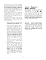
PIPES++
USER MANUAL
Watercom Pty Ltd
15 Little River Close
Wooli NSW 2462
Australia
Phone 612 6649 8005
[email protected]
TABLE OF CONTENTS
TABLE OF CONTENTS
1 OVERVIEW
1
2 HARDWARE
1
3 GETTING STARTED
1
4 USING THE MOUSE
2
5 MENU COMMANDS
2
File Menu
2
Edit Menu
4
Draw Menu
Rules for Drawing a Pipe Network
Nodes
Reservoirs
Pipes
Kinked Pipes
Minor Head Loss
Pumping Station
Check Valve
Reservoir Inlet Control Valve
Pressure Reducing Valve
Pressure Sustaining Valve
Specialised Control Valve
Combined Inlet Control and PSV
Rate of Flow Control Valve
Valve with % Open vs Time Specified
Valve Opened/Closed by Remote Signal(s)
Sprinkler
View Menu
Drawing Area
Pipe and Node Text and Colors
5
5
5
6
6
7
7
7
8
8
8
8
8
8
9
9
9
9
9
9
10
Options Menu
10
Run Menu
11
Help Menu
11
6 RESULTS
12
Results At a Particular Time
12
Trace Graphs
12
HGL Graphs
12
APPENDIX A
13
WATER QUALITY MODELLING
APPENDIX B
15
CONVERTING WATSYS DATA FILES
Step 1 - Check the Watsys Data File
16
Step 2 - Prepare the Network Diagram
16
Step 3 - Merge the Watsys Data File
17
Step 4 - Enter Other Data
17
APPENDIX C
TECHNIQUES FOR LARGE NETWORKS
18
Fluoride or some other chemical varies with time.
Chemical injection points can be specified with the
chemical concentration specified as data for the
duration of the analysis. Trace graphs are available
for these results also.
1 Overview
PIPES++ is a program that does Single Balance or
Extended Period Simulations of flow and water
quality in a town water supply system.
Components that can be modelled include:
The various graphs can be sent to a printer or plotter
or file or copied via the Clipboard directly to a word
processor (eg Word for Windows) for inclusion in a
report.
 Reservoirs
 Pipes

Pumping Stations
 Minor Head Losses
 Check Valves
2 Hardware
 Reservoir Inlet Control Valves
 Various specialised control valves
You will need a machine with Windows 95, 98, NT,
2000 or XP. You will also need the dongle
supplied with PIPES++.
 Pressure Reducing Valves
 Pressure Sustaining Valves
 Flow Control Valves
 Sprinklers
Pipe flows may be calculated using either the
Colebrook White equation or the Hazen Williams
equation. You draw the network on screen using
lines to represent pipes and pre defined symbols to
represent pumps, valves, reservoirs etc.
If you
already have the pipes drawn in a CAD system (eg
Autocad) you can create a DXF file directly from
that.
3 Getting Started
A CD containing the software and a software lock
are provided. The software lock should be attached
to a USB port on your computer. You should start
Windows Explorer, select the drive containing the
PIPES++ CD, go to the PIPES++ subdirectory and
double click SETUP.EXE. This will install the
software on your hard disk.
Data is entered via dialog boxes, which are
accessed by right clicking on the pipe or symbol,
and selecting Edit Data from the pop up menu.
PIPES++ incorporates an extensive online help
system and we encourage you to use it. You can
access the help system from the Help menu, or by
pressing F1, or using the Toolbar help button.
Clicking the Toolbar help button puts PIPES++ into
help mode. You can then click on any object (eg a
menu item, another symbol in the toolbar, a pipe, a
node etc) to get specific help on that object.
Extended Period simulations (typically for 24
hours) can be carried out and during the simulation
pumps can be started and stopped and valves
opened and closed based on control rules which you
specify (eg when a reservoir fills, stop a pump;
when it falls 2 metres start the pump). Results can
be displayed in several ways including
 Detailed results shown on a network
diagram at any time during the simulation
You might like to experiment with the sample data
file SMALL.DAT which is supplied with
PIPES++.
 Trace graphs showing how a value varies
with time (eg flow in a pipe, HGL at a
node, Water Level in a reservoir).
 Minimum and maximum pressure occurring
at each node at any time during the
simulation.
Water quality analyses can also be carried out to
simulate how the concentration of Chlorine,
1
from another PIPES++ file to the current diagram.
The merging file must have two nodes in common
with the current diagram so that PIPES++ can
determine the correct orientation and scaling for the
file to be merged.
4 Using the Mouse
Clicking on a shape, such as a node or pipe, will
highlight it. You can perform various operations on
a highlighted shape such as deleting it or moving it
around the screen. To move a highlighted shape
you drag it using the mouse.
Import DXF or DWG file allows you to read
information stored on a DXF or DWG file. These
files can be created by most CAD packages. If you
already have pipes shown on a CAD drawing this
feature will save you some time in drawing a
network and entering pipe data. You will be
prompted to select the Pipe layer name and the
Node layer name. PIPES++ will interpret all
straight lines and circles on these layers of the DXF
file as pipes and nodes respectively. This means
that no other straight lines or circles can be drawn
on these layers. It is not necessary to draw all pipes
and nodes on the DXF file. You can add pipes and
nodes later from within PIPES++.
To open a dialog box relating to a shape right click
on the shape and select Edit Data from the pop up
menu. For example, in the dialog box for a pipe
you can enter the pipe length, diameter, roughness
etc. and view results of the analysis.
5 Menu Commands
You will also have the option of specifying a
background layer. This would normally contain
street and property boundaries, street names etc.
This layer can be shown or hidden from within
PIPES++. Its colour can also be changed. The
default colour of light grey allows it to be seen
while keeping the pipes and nodes visually
dominant. If you have previously imported a DXF
file without a background layer, you can import the
background layer only at a later time. This
operation requires that the drawing area has not
been extended or cropped since the DXF file was
imported. If it has been, you will need to
temporarily crop or extend it to return to the
original borders while you import the background
layer. You can then extend or crop it without losing
pipes and nodes.
All of the Menu Commands can be accessed from
the menu bar shown in the figure below. In
addition many of the Commands can be accessed
from the tool bar below the menu bar. The
Commands behave in the same manner regardless
of how they are accessed.
File Menu
You will be asked if the DXF drawing is drawn to
scale. If you answer yes, PIPES++ will assign a
length to all pipes based on the length you enter for
one pipe.
Nodes can be represented in the DXF file by a
simple circle drawn on the node layer, or by a block
inserted on the node layer. If you want PIPES++ to
read node labels from the DXF file the node must
be represented by a block. The block should be set
up as follows:
Many of the choices available from the File menu
are common to most Windows Applications
 the block should contain a circle and a text
attribute only
Open allows you to open a new file.
 the centre of the circle should be at (0,0)
If you insert a block to represent a node in the DXF
file you will be prompted for a text value. You
should enter the node label here.
The file
NODE_SYM.DXF, provided with PIPES++, can be
Close allows you to close the current drawing,
ready to start a new network.
Merge Another File allows you to add the details
2
field blank. If you are working on a job previously
exported from PIPES++ there will be numbers in
this field. You should not change or delete these
numbers.
used to define the block.
Pipes are represented by lines drawn on the pipe
layer of the DXF file. If you draw a series of lines,
with their ends touching, PIPES++ will interpret
them as a kinked pipe. A circle (or circle in a
block) at the end of a line will fix the end point of
the pipe.
Merge Watsys Data File allows you to extract pipe
and node data from an existing Watsys data file and
merge it with the current diagram. See Appendix B
for more details.
If you are working with a file where pipes and
nodes are present, this menu item will appear
instead as Import / DXF or DWG background
file. As from June 2003 you will have the option of
either adding this background to an existing
background or replacing it.
Export / DXF allows you to create a new DXF file
of the pipes and nodes or to update an existing file.
You might wish to update an existing drawing if
you have changed the number or location of pipes
while working in PIPES++. If you update an
existing DXF file, the information on other layers
will be retained unchanged.
Import / Mapinfo files allows you to import data
from Mapinfo MID/MIF files. This capability is
part of the GIS Interface Module that is sold
separately from the main PIPES++ software. Two
sets of MID/MIF files are required; one for nodes
the other for pipes. A DXF file containing the
background layer can be imported at the same time.
There are file naming conventions and field name
conventions that you must follow. The easiest way
to see these is to export a set of Mapinfo files from
a small example and inspect the files generated.
There will be 4 files called eg MyJob_Nodes.mid,
MyJob_Nodes.mif,
MyJob_Pipes.mid
and
MyJob_Pipes.mif. If a background layer is present
there will be a 5th file called MyJob.dxf. Most of
the fields in the MID/MIF files are self explanatory.
You should not edit or change the PIPESid field. If
you are starting a new job you should leave this
field blank. If you are working on a job previously
exported from PIPES++ there will be numbers in
this field. You should not change or delete these
numbers.
DXF files produced by PIPES++ do not contain
blocks. In these files pipes are represented by lines
and nodes are represented by circles. These can be
on different layers if you wish. One text value can
be written for pipes (diameter or length or flow etc),
and one text value can be written for nodes (label or
HGL or pressure etc). If you need more than one
text value you can write a second DXF file and later
merge them in your CAD program.
Export / Mapinfo files allows you to export data
and results to Mapinfo MID/MIF files. This
capability is part of the GIS Interface Module that is
sold separately from the main PIPES++ software.
The procedure is straightforward. A set of 4 files
will be created; 2 files for pipe data and 2 files for
node data. If a background layer is present a DXF
file will also be created. If results are available in
the PIPES++ model these will be included in the
files and you will be asked for a brief title (eg you
might use 20 to indicate results are for the year
2020). This allows you to build up sets of results
(minimum pressure and HGL, maximum pipe
flows) for various years in your GIS. You can do
several runs in PIPES++ and export them to the
same MID/MIF files. Depending on the title you
supply, PIPES++ will either add new fields or
update existing fields.
Import ESRI Shapefiles allows you to import data
from sets of SHP/SHX/DBF files. This capability is
part of the GIS Interface Module that is sold
separately from the main PIPES++ software. Two
sets of shapefiles are required; one for nodes the
other for pipes. A DXF file containing the
background layer can be imported at the same time.
There are file naming conventions and field name
conventions that you must follow. The easiest way
to see these is to export a set of shapefiles from a
small example and inspect the files generated.
There will be 6 files called eg MyJob_Nodes.shp,
MyJob_Nodes.shx,
MyJob_Nodes.dbf,
MyJob_Pipes.shp,
MyJob_Pipes.shx
and
MyJob_Pipes.dbf. If a background layer is present
there will be a 5th file called MyJob.dxf. Most of
the fields in the DBF files are self explanatory.
You should not edit or change the PIPESid field. If
you are starting a new job you should leave this
Export ESRI Shapefiles allows you to export data
and results to ESRI shapefiles. This capability is
part of the GIS Interface Module that is sold
separately from the main PIPES++ software. The
procedure is straightforward. A set of 6 files will
be created; 3 files for pipe data and 3 files for node
data. If a background layer is present a DXF file
will also be created. If results are available in the
PIPES++ model these will be included in the files
and you will be asked for a brief title (eg you might
use 20 to indicate results are for the year 2020).
3
This allows you to build up sets of results
(minimum pressure and HGL, maximum pipe
flows) for various years in your GIS. You can do
several runs in PIPES++ and export them to the
same MID/MIF files. Depending on the title you
supply, PIPES++ will either add new fields or
update existing fields.
change to indicate the type of action to be affected
(eg Undo might change to Undo Edit Data).
Find a Node allows you to easily locate a node in
the network. This is useful on large drawings,
especially if you are not very familiar with the
network.
Find ????? allows you to find a shape for which
data is incomplete. This is useful on large drawings
if PIPES++ cannot calculate results because there is
some shape for which data is incomplete, but you
don’t know which shape it is.
Print allows you to print:
 the network diagram showing node labels
and pipe diameters
 the current diagram as shown on screen.
You can adjust the information shown on
screen (eg pipe flow or velocity or diameter
or length etc, node label or HGL or pressure
etc) from the View / Pipe Text and Colours
menu.
Copy Data to Spreadsheet will copy the current
pipe and node data to the clipboard. You can then
paste this data into a spreadsheet by placing the
cursor in cell A1 of the spreadsheet and selecting
Edit / Paste. You can then format the data to make
it more readable. You might make the headings
bold, center the text in cells containing numbers etc.
 a summary of the current data. This,
together with a current network diagram, is
useful for documenting your work.
Copy Results to Spreadsheet will copy the current
pipe and node results to the clipboard. You can
then paste these results into a spreadsheet. This is
useful for large networks where it can be difficult to
identify nodes with low pressures, pipes with high
friction losses or velocities. With the results shown
in a spreadsheet you can use the spreadsheet’s
capabilities to quickly identify problem areas. For
example, you can sort the node results based on
pressure to see all the problem pressures. You can
also sort the results based on pipe friction slope to
identify the best candidates for augmentation to
overcome low pressure problems.
 a summary of results at the current time (as
shown in the box at top left of network
diagram).
 a network diagram showing the minimum
HGL which occurred at each node at any
time during the simulation.
 a network diagram showing the minimum
pressure which occurred at each node at any
time during the simulation.
 a network diagram showing the maximum
pressure which occurred at each node at any
time during the simulation.
Before printing, you will have the opportunity to
change printer settings (eg Landscape or Portrait
mode, which printer to use etc).
Paste Data from Spreadsheet can be used to edit
the data in a spreadsheet, add new pipes and nodes,
or even to create a new network directly from data
entered into a spreadsheet. It is recommended that
you first paste data into a spreadsheet. You can
then edit the data. For example you might change
some pipe diameters and add levels and demands to
nodes. When you are satisfied with the changes
you select (highlight) all the rows from row 1 to the
last row of pipe data. Then you select Edit / Copy
to copy the data to the clipboard, then use Alt-tab to
switch to PIPES and select Edit / Paste Data from
Spreadsheet. Any changes that you have made in
the spreadsheet will then be made within PIPES and
any new pipes or nodes that you added in the
spreadsheet will be created in PIPES.
Exit will close PIPES++. If you have made
changes to the current network you will be asked
whether you wish to save them.
Below Exit is a list of up to 4 of the most recently
opened files. Clicking on one of these files is the
easiest way to open a file you were recently using.
Edit Menu
If you add a new node in the spreadsheet you will
need to provide an x,y coordinate for it. If you
change a pipe type the text must exactly match a
pipe type in PIPES data base. The safest way to do
this is to copy a pipe type from another cell and
paste it into the cell to be changed.
Undo and Redo can be used to change recent
actions such as drawing new shapes, moving
shapes, deleting shapes and editing data for a shape.
When these menu items become active the text will
4
Copy Current Diagram will copy the network
diagram to the Clipboard. You can then paste it
into your Windows Word Processor or Windows
Drawing Program for inclusion in a report.
well as various specialised control valves in your
network.
Alternatively, you can draw the more common
components (nodes, pipes, reservoirs, pumps and
check valves) using the Toolbar.
Delete allows you to delete a pipe, pump valve etc.
First you click on the item to highlight it. You can
then press the Del key or select this menu item to
delete it.
Before discussing these items in detail, there are
some rules which you must follow in drawing a
pipe network. These are:
Job Description allows you to document this job in
detail. You can enter notes such as new pipes
included in this analysis, the fact that this analysis
uses Peak Day Demands for Year 2000 etc.
 reservoirs and sprinklers are located at a
node. That is, the base or corner of these
items should just touch one node. If there
is too big a space between the item and its
node, PIPES++ will not associate the item
with that node.
Title Block allows you to edit the text which
appears in the bottom right of the drawing. This
text may not always be visible on the screen. If you
pan to the bottom right of the drawing (using the
arrows or sliders on the bottom and right of the
drawing) you will see the text. If you do not want
to show a title block you can simply delete all three
lines of text.
 pipes are located between two nodes. That
is, each end of a pipe should just touch one
node. If there is too big a space between
the end of a pipe and its node PIPES++ will
not associate the pipe with that node.
 minor head losses, pumping stations and all
types of valves are located between two
nodes. That is, you should draw two nodes,
one on each side of these items. The space
between the item and its nodes is not
important, but about 5 mm is recommended
for appearances sake.
You will be
prompted to supply the name of the
upstream and downstream node in a dialog
box.
Pipe Data Base allows you to edit the pipe data
base. The data base contains internal diameters for
a range of common pipe materials and classes. You
can add or remove pipe types and pipes. The pipe
data base was introduced with Version 95.20. If
you are using data files prepared with an earlier
version of PIPES the data base feature will be
temporarily disabled.
Draw Menu
Rules for Drawing a
Pipe Network
Nodes
A node is shown as a small circle on the network
diagram. It is an essential part of the network
diagram and is used as follows:
The Draw menu is used to enter the details of your
pipe network. A glance at this menu will show that
you can include nodes, reservoirs, pipes, minor
head losses, pumping stations, check valves,
reservoir inlet control valves, pressure reducing
valves, pressure sustaining valves and sprinklers as
 pipes are drawn from one node to another
node
5
 valves, pumping stations and minor head
losses are drawn between two nodes
reservoirs and sprinklers are drawn touching one
node To draw a node:
You can click on the Quality Details button to edit
data for a water quality analysis. Water quality
modeling is discussed in more detail in Appendix
A.
 select Node from the Draw Menu, or click
on the node button in the Toolbar
Hint: You can keep your drawing looking tidy by
moving the node label (simply drag it with the
mouse). When results have been calculated the
label will be replaced by the HGL value which may
require a little more space. If necessary you can
drag the HGL value to suit.
 place the mouse cursor where you want the
node
 press and hold down the left mouse button
 you can move the mouse to place the node
precisely. When the node is correctly
located release the mouse button
Hint: To draw several nodes hold down the Shift
key as you release the mouse button. You will then
be ready to draw another node immediately.
Reservoirs
Selecting Reservoir, or clicking the Reservoir
button in the Toolbar, allows you to draw a
reservoir. When you do this you will notice ?????
appears beside the reservoir. This indicates that
some data is required for the reservoir. Right click
on the reservoir and select Edit Data to display a
dialog box showing the required data. You can now
enter this data.
The procedures described here for drawing a node,
apply to the various other network components.
The use of the Shift key applies to nodes and pipes
only.
Reservoirs can have a constant area (eg cylindrical
tanks) or the area can vary with depth (eg a
spherical tank). A constant level reservoir is a
special type of reservoir.
Data for a node is optional. You can specify the
elevation at the node and you can specify details
about demand from the node. To enter data for the
node, point to it, right click and select Edit Data
from the pop up menu. A dialog box will appear
and you can enter data for elevation, and demand
details.
If you have drawn the reservoir at a node (as you
should) PIPES++ will show the node label in the
title bar of the dialog box (eg Reservoir at Node
N1). If the reservoir is not drawn at a node, the title
bar will show Reservoir at Node ????.
Demands from a node are allocated to one of ten
areas. Each area can have a different:
When PIPES++ is satisfied that all essential data
has been specified for the reservoir, and that the
reservoir is drawn close to a node, the ????? will
disappear from the drawing. If you have specified a
name for the reservoir, this name will appear in
place of the ?????.
 multiplying factor which is applied to all
demands in that area
 day to day variation in demand. The day to
day demand pattern is a set of numbers.
There is one number for each day for up to
32 days. The first number is applied as
multiplying factor to demands for day 1 in
the simulation, the 2nd to day 2 etc.
Pipes
Selecting Pipe, or clicking the pipe button in the
Toolbar, allows you to draw a pipe. Point to the
pipe starting point and depress the left button (don’t
release it yet). Now move the mouse and you will
see the pipe follow the mouse movement. When
you are satisfied with the pipe location release the
left button.
 diurnal demand variation pattern. This is a
set of 48 numbers giving the ratio of
demand to average demand at half hourly
intervals over a full day. The total of all the
numbers should be 48.0.
 fire demand. For a residential area, you
might specify a fire demand of 11L/s. For
an industrial area you might specify 22 L/s.
The fire demand is used only when you
choose Fire Flow Analysis from the Run
menu. The fire flow analysis is described
in more detail in that section.
In the main data dialog box for a node you can
press the Area details button to edit these values.
Not satisfied with the location? Highlight the pipe
(simply click on it). You can now drag the entire
pipe or drag only one end. To drag the entire pipe,
point near the centre of the pipe and drag from
there. To drag one end, point to that end and drag
it.
Hint: To draw many pipes hold down the Shift key
as you release the mouse button. You will then be
6
Minor Head Loss
ready to draw another pipe immediately.
A minor head loss should be drawn between two
nodes. Minor head losses can be used to model
anything which has a head loss proportional to flow
squared.
You can enter data for pipes by right clicking on the
pipe, and selecting Edit Data, to bring up the dialog
box. When all data is specified, and both ends of
the pipe are touching a node, the ????? will be
replaced by the diameter (unless you have requested
some other item of data from the View/Pipe Details
menu). If the text associated with a pipe (????? or
diameter etc) is badly located you can simply drag
it elsewhere.
Headloss = a.Q2
The data required is the nominal diameter and K
where
Headloss = KV2 / 2g
The dialog box will allow you to enter:
You can draw a minor head loss, enter data for it
and inspect the results of an analysis as you would
for any network component.
 Length
 Pipe type (eg uPVC class 9)
 Diameter
Pumping Station
 Whether to use the default value of
roughness or some other value
A pumping station should be drawn between two
nodes. A pumping station can contain several
different pumps and these pumps can be started and
stopped by signals from pressure sensors and level
indicators located anywhere in the system. You
assign a priority from 1 (highest) to 5 (lowest) to
each signal. If a pump receives two conflicting
signals (one telling it to start, the other telling it to
stop) it will obey the higher priority signal. If both
signals have the same priority, it will stop.
 Details of minor head losses (valves and
fittings) to be included with the pipe
 Water Quality Data. Press the Quality Data
button to open a dialog box in which you
can specify these data
Hint: It is simpler to lump valve and fitting losses
in with a pipe rather than to model them as a
separate minor head loss.
Pumps can also be instructed to stop during
specified time periods. You can specify a period
such as 1800 to 2200 (6 pm to 10 pm every day), or
2:1800 to 2:2200 (6 pm to 10 pm on day 2 of the
simulation only).
When you first open the dialog box for a new pipe
you will see a value suggested for diameter. You
can change this value if necessary. The suggested
value is the same as for the most recently entered
pipe.
A set point controller can also be specified for a
variable speed pump.
This controller will
automatically adjust the pump speed (from 1% to
100% of full speed) to maintain the HGL at a
specified node at a set value. If a speed greater than
100% would be required to maintain the HGL at the
set level, it will not be maintained.
If the pipe type and size you wish to use are not
available in the pipe data base you can edit the data
base and add the pipe details. Click on Edit / Pipe
Data Base to add more pipes.
Kinked Pipes
You may wish to draw a pipe as a series of straight
lines (eg when drawing a second pipe between two
nodes). Selecting Pipe with Kinks allows you to
do this. You draw the first segment as you would a
normal pipe. Then move the mouse to draw the
second segment and click once to lock it in place.
Repeat this process for additional segments. Click
with the RIGHT mouse button to lock the last
segment in place.
Variable speed pump control is the highest priority
signal. In other words all other signals will be
ignored. This is why the other pump controls will
be greyed out when you check the Speed Control
box for a pump.
A variable speed pump cannot be controlled from a
node with a reservoir. This is because, at any time
during the simulation, PIPES++ calculations will
vary the pump speed until the correct HGL at the
control node is achieved. If there was a reservoir at
the control node, the HGL would be fixed at the
current water level regardless of the pump speed,
and PIPES++ would be unable to determine a
suitable pump speed.
After you have drawn it, a kinked pipe is very
similar to a normal pipe. The only difference is that
you can drag the kinks as well as the ends.
7
If you wish to control a variable speed pump from a
node which has a reservoir, simply leave out the
reservoir. With a fixed level in a reservoir, there is
clearly no inflow to or outflow from the reservoir.
This means that the reservoir storage is not used
during the simulation and it might as well not be
there. By leaving it out you allow PIPES++ to
assess the effect of varying speeds on the HGL and
hence determine the correct pump speed.
Pressure Reducing Valve
A pressure reducing valve should be drawn between
two nodes
A pressure reducing valve will
automatically throttle flow to limit the maximum
downstream pressure to a preset value. The data
required is the downstream HGL setting, the
nominal diameter and K where
Headloss = KV2 / 2g
The variable speed pump controller will not work
well if the control node is very close to a reservoir.
The pump is likely to hunt between full speed and
zero speed because variations in reservoir water
level (eg from 6am to 6.30am) have a more
significant effect on HGL at the control node than
variation in the pump speed can exert at one instant
(eg 6.30am). In this case you might consider
controlling from the reservoir node, and leaving the
reservoir out of the network model.
You can draw a pressure reducing valve, enter data
for it and inspect the results of an analysis as you
would for any network component.
Pressure Sustaining Valve
A pressure sustaining valve should be drawn
between two nodes A pressure sustaining valve
will automatically throttle flow to sustain the
upstream pressure at a preset minimum value. The
data required is the upstream HGL setting, the
nominal diameter and K where
Electricity tariffs can be specified for a pumping
station. The cost of energy and KVA charges will
then be calculated during a simulation.
Headloss = KV2 / 2g
You can draw a pressure sustaining valve, enter
data for it and inspect the results of an analysis as
you would for any network component.
You can draw a pumping station, enter data for it
and inspect the results of an analysis as you would
for any network component.
Specialised Control Valve
Check Valve
Various specialised control valves are supported by
PIPES++. These valves are occasionally used in
modelling of water supply distribution systems.
They include:
A check valve should be drawn between two nodes
Check valves will allow flow in the forward
direction only. They will close to prevent reverse
flow if necessary. The data required is the nominal
diameter and K where
 Combined Inlet Control and Pressure
Sustaining Valve
Headloss = KV2 / 2g
 Valve which restricts the flow to a preset
maximum value
You can draw a check valve, enter data for it and
inspect the results of an analysis as you would for
any network component.
 Valve with position specified as a function
of time
Reservoir Inlet Control Valve
 Valve which is opened / closed by remote
signal(s). The valve can be opened and or
closed by signals from flow meters,
pressure sensors and level indicators
located anywhere in the system.
A reservoir inlet control valve should be drawn
between two nodes A reservoir inlet control valve
is used to prevent a reservoir overflowing during an
Extended Period Simulation (EPS). The data
required is the nominal diameter and K where
Combined Inlet Control and
PSV
Headloss = KV2 / 2g
You must also provide details for controls. (ie the
location of the controlling reservoir and reservoir
levels which cause the valve to open and close).
A combined Inlet Control and Pressure Sustaining
Valve combines the functionality of a Reservoir
Inlet Control Valve and a Pressure Sustaining Valve
in the one valve.
You can draw a reservoir inlet control valve, enter
data for it and inspect the results of an analysis as
you would for any network component.
8
Rate of Flow Control Valve
Sprinkler
A rate of flow control valve should be drawn
between two nodes This valve will automatically
throttle flow to limit the maximum flow to a preset
value. The data required is flow setting, the
nominal diameter and K for a fully open valve
where
A sprinkler should be drawn touching one node.
The data required is the elevation (RL) of the
nozzle and the flow at some pressure.
You can draw a sprinkler, enter data for it and
inspect the results of an analysis as you would for
any network component.
Headloss = KV2 / 2g
View Menu
You can draw a Rate of Flow Control valve, enter
data for it and inspect the results of an analysis as
you would for any network component.
Valve with % Open vs Time
Specified
This valve should be drawn between two nodes
The data required is the nominal diameter and K for
the valve in the fully open position where
Headloss = KV2 / 2g
You must also provide details for controls. (ie a
table showing the valve % open for various times
during the day).
You can draw this valve, enter data for it and
inspect the results of an analysis as you would for
any network component.
Drawing Area
You have probably realised by now that you cannot
hope to fit a large pipe network on a single screen.
When you start a new drawing PIPES++ allocates a
drawing area the size of 4 screens (2 vertically by 2
horizontally). In other words, when you start
PIPES++ you are looking at the top left hand
quarter of the available drawing area.
Valve Opened/Closed by
Remote Signal(s)
This is a general purpose valve which can be used
to model many different situations. The valve is
either fully open or fully closed. It can receive
signals from pressure sensors and water level
indicators located anywhere in the system. You
assign a priority of 1 (highest) to 5 (lowest) to each
signal. If the valve receives conflicting signals
from two sensors (one telling it to open, the other
telling it close) it will obey the higher priority
signal. If both signals have the same priority, it will
close.
Selecting Index Sheet allows you to quickly locate
the viewing window precisely where you want it. If
you find yourself getting lost looking at a small part
of a large drawing this will be helpful. When you
select Index Sheet, you will see the entire drawing
on one screen and a dashed rectangular box. This
box indicates the position of the normal view
window. You can drag this box wherever you want
to position the normal view window. Releasing the
left mouse button will return you to the normal
view window.
This valve should be drawn between two nodes
The data required is the nominal diameter and K for
the valve in the fully open position where
HGL Graph will show a graph of HGL along one
or more pipes at the current time (1:0500 - ie 5am
on day 1 in the figure). You can nominate the
nodes along each pipe route.
Headloss = KV2 / 2g
You must also provide details for controls. These
vary depending on which control signals you use.
The data entry dialog boxes are self explanatory.
Zoom is useful if you find your drawing is too
cluttered or too spread out. This can happen when
you read a DXF file or if you are inexperienced in
drawing a network diagram in PIPES++. You will
be prompted for a magnification factor.
You can draw this valve, enter data for it and
inspect the results of an analysis as you would for
any network component.
9
Extend Drawing Area. This is like sticking more
paper to your drawing. The size of your entire
drawing area increases, but you can see no more on
one screen (ie the size of the view window does not
change). If you work with large networks, sooner or
later you will find that the 4 screens of drawing area
are insufficient and you will need to extend the
drawing area.
draw a network this text shows the node labels and
the pipe diameters. After you calculate results, the
text shows the node HGLs and the pipe flows.
Using Node Text and Colors and Pipe Text and
Colors you can change this text to show other data
or results.
You can also use these menu items to colour code
the results. For example, selecting Node Text and
Colors shows the dialog box in the figure below.
The user has then specified that the HGL should be
displayed at each node and that the nodes should be
colour coded based on the value of pressure. In this
example, the user has specified pressures up to 12m
should be red, 12 to 20 should be cyan, 20 to 125
should be yellow, and greater than 1250 should be
green.
Crop Drawing Area allows you to trim the edges
of the drawing area. You can crop right down to
the size of one screen full.
Extending or Cropping the drawing area adds or
subtracts one half a screen width and height each
time you do it. If you inadvertently lose some of
your network when you Crop the drawing it will
reappear if you Extend the drawing.
Trim Drawing Edges is useful if you find there is
too much white space around a network when you
print it.
Snap Pipes to Nodes causes the pipe ends to be
moved to the centre of the node.
Node Text and Colours allows you to change the
text displayed beside each node. You can show
labels, HGL, pressure, etc. You can also colour
code the nodes to show different pressure ranges in
different colours.
Pipe Text and Colours allows you to change the
text displayed beside each node and to colour code
the pipes. You might choose to colour code the
pipes based on their diameters. This will give a
good indication of the location of major pipes in the
network.
Background can be selected or deselected to show
or hide the background layer. A check mark
indicates when the background is selected.
Background Colour allows you to change the
colour of the background layer.
Options Menu
Toolbar can be used to show or hide the Toolbar.
The check mark indicates that the Toolbar is
currently visible.
Flow Units allows you to choose between various
units. You should select your preferred option
before entering data for pumps, valves, demands
etc.
Status Bar can be used to show or hide the Status
Bar. The check mark indicates that the Status Bar
is currently visible.
Headloss Formula allows you to choose between
the Hazen Williams and Colebrook White formulae
for headloss in pipes. The data entry dialog box for
pipes will ask for either C or k depending on which
equation you have specified. You should choose
the formula you prefer before entering data for
pipes.
Pipe and Node Text and
Colors
When you draw a network there is some text
associated with each node and pipe. When you first
10
The Hazen Williams equation is described in most
standard hydraulic texts. The Colebrook White
equation is:
Fire Flow Analysis starts a fire flow analysis. The
non-fire demands are those appropriate for the
starting time specified under the Options /
Simulation Period menu item. Reservoir levels and
pump and valve status are the initial values
specified in the data or those appropriate at the
simulation starting time. In a network with 1000
nodes there will be 1000 separate analyses done,
with a fire at a each node in turn. In each node data
dialog box, the default radio button under For Fire
Flows is Use dominant area. Consider a node with
some residential demand (area 1) and some
industrial demand (area 2), and let us assume we
have specified a fire demand of 11L/s for area and
22L/s for area 2. In this case the dominant area will
be area 2 (because 22 > 11L/s) and the fire demand
will be 22L/s when PIPES++ simulates a fire at this
node. Consider another node that has residential
demand only (area 1). In this case the dominant
area will be area 1 and the fire demand will be
11L/s when PIPES++ simulates a fire at this node.
If this logic does not suit you, then you can specify
which are to use for the fire demand. For example,
if a node had both residential and industrial demand
but you wanted to simulate a fire in the residential
area with 11L/s you would click on You specify
area and choose 1 (for area 1) in the drop down box
that appears.
 k
2.51v 
V  2 2 gDS log 


 3.7 D D 2 gDS 
where V = velocity of flow
g = acceleration due to gravity (m/s2)
D = pipe internal diameter (m)
S = slope of Hydraulic Grade Line
k = pipe wall roughness (m)
v = kinematic viscosity of fluid (m2/s)
The Colebrook White equation is considered to be
more accurate than the Hazen Williams equation
and has the added advantage that roughness values
(k) do not vary with pipe diameter. In the days of
slide rules the Hazen Williams equation was
preferred because it was easier to use. Computers
have no problem using the Colebrook White
equation and it is recommended over the Hazen
Williams equation.
Simulation Period allows you to specify either a
single balance run or an Extended Period
Simulation (EPS). If you select a single balance run
you need to specify only the staring time (eg 0500
for 5am). The starting time is significant because
demands can be different at different times of the
day. If you select EPS you will also need to specify
the duration of the simulation (eg 1 day).
When the analysis is complete the HGL (or
pressure) will be the minimum due to a fire
anywhere in the network. This may be due to a fire
at another node. For example the minimum HGL at
a node in a residential area may not be due to a fire
there, but due to a fire in a nearby industrial area.
You can get more information on the worst fire
locations by copying the results to a spreadsheet
(and then choose Edit/Paste in the spreadsheet).
Hint: Sort the spreadsheet based on the minimum
pressure column to quickly check for unsatisfactory
results.
Water Quality Analysis allows you to select either
Chlorine, Fluoride or some other substance to be
modelled. A dialog box appears in which you can
also specify the default initial concentrations for all
nodes and reservoirs and the default bulk and pipe
wall decay rates. Water quality modeling is
discussed in more detail in Appendix A.
There will be no results shown for pipes, pumps or
valves for a fire flow analysis because these vary
depending on the fire location.
Run Menu
Hydraulic Analysis starts an hydraulic analysis.
This menu item will be grey until all data is
complete and only then will you be able to select it
to start an analysis. If ????? appears beside any
network component it indicates that the data for that
component is incomplete. It could also indicate that
a reservoir or sprinkler is not located at a node, or
that one or both ends of a pipe are not touching a
node.
Quality Analysis starts a water quality analysis. If
you have not already carried out an hydraulic
analysis, this will be done automatically before the
quality analysis commences.
A detailed description of how to inspect the results
of an analysis is given in Section 6.
Index is like the index at the back of a book. It
shows a dialog box in which you can search for key
Help Menu
Table of Contents is like the Table of Contents of
a book. It shows topics covered by the help system.
11
words, which are listed in alphabetical order.
Using Help is an introduction to the help system.
Trace Graphs
About PIPES++ shows copyright information and
the version number of PIPES++.
Trace graphs provide a very powerful tool to assist
you in rapidly gaining a good understanding of how
a water supply distribution system performs.
When the analysis is completed you can view trace
graphs. You can display the trace graph for a
network component by right clicking on the
component (eg point to a reservoir and click the
right mouse button) and select the desired graph
from the pop up menu.
6 Results
After calculating results for a simulation, you will
be able to inspect the results at any time during the
simulation. You will also be able to view trace
graphs.
Results At a Particular
Time
To inspect detailed results at a particular time select
the time in the Time Window at the top left of the
drawing area. Results will be displayed on the
network diagram for every pipe and every node. By
default, the flow in each pipe and the HGL at each
node will be shown. You can control what results
are shown by selecting Pipe Text and Colors or
Node Text and Colors from the View menu.
You can show several graph windows on screen at
the same time. You can move these windows
around the screen and re-size them to compare the
behaviour of different trace values.
You can print graphs or copy them to the Clipboard
from the File and Edit menus in the graph window.
HGL Graphs
You can plot the HGL along one or more pipes by
selecting HGL Graphs from the View menu.
You can specify any pipe route for plotting an HGL
graph. If you have specified a level for every node
along the route the ground level will also be plotted.
You can right click on any network component,
and select Edit Data, to see the complete results for
that component at the selected time.
12
Appendix A
WATER QUALITY MODELLING
13
The water quality model in PIPES++ tracks a
dissolved chemical as it flows through the network.
It uses the conservation of mass equation to
calculate the concentration of dissolved chemical at
each node and at internal points along pipes. Initial
concentrations must be specified for each node. In
addition nodes and reservoirs can be nominated as
injection points. For these points, the chemical
concentration versus time must be specified.
taken as an indication of the amount of water
coming from the source where Fluoride was
injected. For example a Fluoride concentration of
40 mg/L at node X would indicate that 40% of the
water at node X came from S1. For this analysis a
non decaying chemical is required, and Fluoride is
convenient.
It is stressed that Water Quality modeling is not an
exact science. The process of chlorine decay and
TTHM (total trihalomethanes) growth in water
distribution systems is not well understood and
much research in this area is taking place around
the world. We expect that the water quality model
described above will be modified as this research
proceeds.
PIPES++ can model decaying chemicals (eg
Chlorine), growth chemicals and conservative
chemicals (eg Fluoride). Growth chemicals are
treated as negative decay chemicals and
conservative chemicals are treated as zero decay
chemicals. The rate of decay is determined by a
first order reaction rate model which allows for
different decay rates close to the pipe wall and in
the bulk flow further away from the pipe wall. For
each pipe a Bulk Decay Rate (per day) and a Wall
Decay Rate (m/day) must be specified. Normally
you would specify the same rate for many of the
pipes in a network and you need then only specify
the default value to be used for these pipes.
At present there are no guidelines available for
selecting reasonable values of bulk and wall decay
parameters for a particular water distribution system
and field testing is generally required. However, as
a starting point, values around 0.03 to 0.5 day-1 and
0.3 to 1.5 m/day for Chlorine bulk and wall decay
rates respectively have been mentioned in the
literature in relation to treated water distribution
systems.
Chemical transfer between the two regions is
calculated by PIPES++ using theory described in
“Transfer Processes”, Edwards, Denny and Mills,
McGraw-Hill, New York, 1976.
In PIPES++ you can select the chemical to be
modelled and specify default values for bulk decay
rate and pipe wall decay rate by selecting Water
Quality Analysis under the Options menu item.
You can also specify the default initial
concentration for all nodes from here. If you wish
to use different values for a particular pipe or node
you can double click on that pipe or node and then
click on the Quality Data button.
The rate of change of concentration at a point is
calculated as:
dc/dt = -Kc
where
c = concentration (mg/L)
t = time (days)
K = an overall constant at this location as follows
K = kb + kw.kf/ (Rh(kw + kf))
where
kb = bulk decay rate (supplied by you)
kw = wall decay rate (supplied by you)
Rh = pipe hydraulic radius (calculated as Pipe
Diameter / 4)
kf = mass transfer coefficient (calculated by
PIPES++)
PIPES++ can also be used to trace the source of
water in multi source systems. You can specify an
initial Fluoride concentration of zero at all nodes
except for one source node (say S1) where Fluoride
will be injected to maintain the Fluoride
concentration at 100 mg/L. After allowing time for
the system to come to equilibrium, which may be
some days depending on the size of network and the
demand level, the Fluoride concentration can be
14
Appendix B
CONVERTING WATSYS DATA FILES
15
its own Daily Demand Factor Sequence Number.
For example, Area No.3:
Introduction
If you wish to convert a WATSYS data file you will
need to prepare a network diagram having the same
node labels as the Watsys data file. You can then
merge the WATSYS data file into the current
network diagram and the data for pipes and nodes
will be automatically converted. You will need to
re-enter the data for reservoirs, pumps, valves etc
from within PIPES++.
 can use any (one) Demand
Multiplying Factor (eg 0.15)
 must use Daily Curve Sequence
Number 3 (and no other)
 must use Daily Demand Factor
Sequence Number 3 (and no other)
You will likely need to renumber Demand Areas
and/or Daily Curve Sequence Numbers and/or
Daily Demand Factor Sequence Numbers to comply
with these requirements before you attempt to
merge a WATSYS data file in PIPES++.
Step 1 - Check the
Watsys Data File
The data for pipes should convert without any
problems. However, there are some things you
should know about the data for nodes and demands
at nodes.
Beware of the default behaviour of WATSYS! If
the Daily Curve Sequence Number and the Daily
Demand Factor Sequence Number are not explicitly
defined, they default to 1. This is correct for Area
1, but incorrect for all other Areas. You must
explicitly define them for any Areas Nos. other than
1, which are used.
PIPES++ does not support Systems in the same
manner as Watsys for DOS. If you have only one
system in your old Watsys data file you should
ensure the data file does not contain the line:
**SY etc
If the Demand Multiplying Factor is not explicitly
defined for an area, it defaults to a value of 1.0.
This is acceptable in PIPES++, but you should be
careful that it is not redefined as a value other than
1.0 elsewhere in the data file.
If you have more than one system in your Watsys
for DOS data file, you will need to label the nodes
in the network diagram to suit the following
convention for merging node labels:
We suggest that you explicitly define the Demand
Multiplying Factor, the Daily Curve Sequence
Number and the Daily Demand Factor Sequence
Number for every area in the WATSYS data file
before you attempt to merge it into PIPES++.
 all node labels in the main system (ie **SY
MAIN) are merged without alteration (ie
node 101 is merged with node 101 on the
network diagram).
 all node labels in other subsystems are
merged with a letter prefixed to the label.
The letter is the first letter of the sub system
name (eg G for **SY ‘GRAVITATION
ZONE’). So node 101 in the Gravitation
Zone would be merged with node G101 on
the network diagram. (ie you need to label
the node on the network diagram as G101).
If you have been using WATSYS, you should be
familiar with the terms Demand Area, and Demand
Multiplying Factor, and Daily Curve Sequence, and
Daily Demand Factor Sequence and Demand
Variation Curve.
If you use two or more sub systems, and the same
Demand Area Number is used in each, check that
the same Demand Multiplying Factor is used for
that Area.
Examples:
The following is correct:
FACTRS 3 0.15 3 :3
4 1.0 4 :4
The following are all incorrect:
FACTRS 3 0.15 2 :3
4 1.0 4 :4
In PIPES++, the term Diurnal Pattern is used
instead of Demand Variation Curve. The terms
Daily Curve Sequence and Daily Demand Factor
Sequence are not normally used. They are used
here only to explain how to convert old data for use
by PIPES++.
FACTRS 3 0.15 3 :3
4 1.0 4 :1
FACTRS 3 0.15 3
4 1.0 4 :4
PIPES++ allows up to 10 demand areas. Each
demand area has its own Demand Multiplying
Factor, its own Daily Curve Sequence Number and
If you are converting a large data file you should
think about the most efficient way to prepare the
Step 2 - Prepare the
Network Diagram
16
network diagram. You can, of course, simply draw
the diagram within PIPES++. If you wish to keep
the network diagram in perspective you will need to
draw the network using a digitiser. If your digitiser
has a Windows driver you can do this directly. If
you have an older digitiser with no Windows driver,
you can digitise the network into a CAD system and
then create a DXF file which can be read into
PIPES++ using File/Read DXF.
Step 3 - Merge the
Watsys Data File
When the network diagram is on screen, with
correct node labels, you can select File / Merge
Watsys data file. If each node and pipe in the
Watsys data file match a node and pipe in the
network diagram (as they should) this should
proceed smoothly. If there are discrepancies (eg a
pipe in the Watsys data file and no matching pipe in
the network diagram) error messages will be
displayed. You should make a note of these error
messages, and adjust either the network diagram or
the Watsys data file until they match.
If you already have a Watsys “map” of the network,
or if you have the pipes drawn in a CAD system, we
recommend that you create a DXF file of the
network diagram and import that into PIPES++
using File/Read DXF.
Before you can merge a Watsys data file, you must
ensure that the node labels on your network
diagram match those in the Watsys data file. There
are several possibilities:
 If you are drawing the network diagram
within PIPES++ you can simply type in the
correct label as you create each node.
Step 4 - Enter Other Data
At this stage the data for pipes, nodes and demands
should be correct. This represents the vast majority
of data in a typical network. To complete the data
you now need to manually enter (ie within
PIPES++) data for pumps, valves, reservoirs,
sprinklers, electricity tariffs and water quality if you
are using these features.
 If you are creating a DXF file within a
CAD program, you can draw each node as a
block with an associated text value for
which you enter the node label (ref page 6).
 If you have a DXF file where the nodes are
drawn as circles and you have (or can
create from a data base) an XY file defining
the label and x,y coordinates for each node,
PIPES++ can read both files and assign the
correct label to each node. When PIPES++
reads a DXF file it checks for the existence
of an XY file of the same name and if it
finds one, it reads node labels from the XY
file. The XY file format must be: Label
xCoord
yCoord
where xCoord and yCoord must match the
values in the DXF file. The XY file must
be an ASCII file.
 If you have a DXF file where the nodes are
drawn as circles and you have no XY file
you can simply read the DXF file.
PIPES++ will automatically create node
labels, but these will not match those in the
Watsys data file and you will need to
manually change each node label within
PIPES++
or
in
a
spreadsheet.
Unfortunately, the node labels in a Watsys
“map” file are floating text and are not tied
in any way to their node. This means they
cannot be used to define node labels in
PIPES++.
17
Appendix C
TECHNIQUES FOR LARGE NETWORKS
18
While using PIPES++ to with large networks we
have developed certain methods of setting up and
checking a model. There are other ways of doing
the same thing, but these are the methods we prefer.
are also shown.
You can select the node results and sort the data in
ascending order of minimum pressure. This will
quickly show all those nodes with substandard
pressures.
Using DXF Files
You can also select the pipe results and sort the data
in descending order of friction slope (m/km).
Excessive values of friction slope indicate that this
pipe is a good candidate for augmentation. They
can also mean that there is an error in the network
diagram forcing this pipe to carry flow which
should be carried by another (possibly larger) pipe.
Another reason for excessive flow in a pipe could
be that reservoir zone valves are incorrectly
modelled.
The first step in setting up a model is to prepare the
network diagram. While this can be done within
PIPES++, for large networks we prefer to import a
DXF file which is produced from a CAD package.
If the DXF file is drawn to scale PIPES++ can
determine the lengths for all pipes after you specify
the length for one pipe. Often the pipes are already
included in a CAD drawing. While this appears to
save some time there are hidden traps in using such
a file. Because every line on a certain layer will be
interpreted as a pipe (or part of a kinked pipe) it is
important that each line is drawn once and only
once, and that there are no stray short lines
accidentally drawn. These errors are easily made
and difficult to detect.
Unless the original
draftsperson was aware of these requirements we
have found it safer and often faster in the long run
to redraw (trace over) all the pipes on a new layer.
Nodes are added on a separate layer to define the
extents of kinked pipes and the interconnection
details. We prefer to let PIPES++ number the
nodes automatically.
Using a Spreadsheet for Editing Data
The next step is to set up demands at nodes. For
large networks we prefer to do this in a spreadsheet
such as Excel. You should copy the data to the
Windows clipboard and then paste it into cell A1 of
a spreadsheet. You can then add demands and
ground levels in the spreadsheet. You can also
change the node labels here if you wish to use a
particular labelling system. When the data is
finalised select all rows from row 1 to the last row
of pipe data and choose Edit / Copy. Then use Alttab to switch back to PIPES++ and choose Edit /
Paste.
Checking Results
In very large models (eg 3000 nodes, 4000 pipes) it
can be a daunting task to look for substandard
pressures and high head loss pipes on the screen or
on a printed diagram of results. To help in
checking results you can select Edit / Copy Results
to spreadsheet, then switch to an empty spreadsheet
and select Paste. The results for the current time
are shown for nodes on the upper part of the
spreadsheet and for pipes on the lower part of
spreadsheet. The minimum pressures and HGLs
which occurred at any time during the simulation
19