Download InSpector 1000 User's Manual

InSpector™ 1000
Digital Hand-Held MCA
User’s Manual
9236111C V1.1
Body: 9236119C
Copyright 2004, Canberra Industries, Inc. All rights reserved.
The material in this document, including all information, pictures,
graphics and text, is the property of Canberra Industries, Inc. and
is protected by U.S. copyright laws and international copyright
conventions.
Canberra expressly grants the purchaser of this product the right
to copy any material in this document for the purchaser’s own use,
including as part of a submission to regulatory or legal authorities
pursuant to the purchaser’s legitimate business needs.
No material in this document may be copied by any third party, or
used for any commercial purpose, or for any use other than that
granted to the purchaser, without the written permission of
Canberra Industries, Inc.
Canberra Industries, 800 Research Parkway, Meriden, CT 06450
Tel: 203-238-2351 FAX: 203-235-1347 http://www.canberra.com
The information in this document describes the product as
accurately as possible, but is subject to change without notice.
Printed in the United States of America.
InSpector and Genie are trademarks of Canberra Industries, Inc.
Adobe and Acrobat are registered trademarks of Adobe Systems in the United States and/or other countries.
Microsoft, Windows and ActiveSync are registered trademarks of Microsoft Corporation in the United States and/or
other countries.
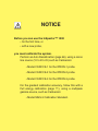
NOTICE
Before you can use the InSpector™ 1000
• for the first time, or
• with a new probe,
you must calibrate the system.
Perform an Auto Recalibration (page 66), using a mono
line source (10 to 20 nCi) such as Canberra’s:
• Model CSRCCS-1 for the IPRON-1 probe.
• Model CSRCCS-2 for the IPRON-2 probe.
• Model CSRCCS-3 for the IPRON-3 probe.
For the greatest calibration accuracy, follow this with a
Full energy calibration (page 71), using a multipeak
gamma source, such as Canberra’s:
• Model MGS-3 Calibration Standard.
Notes
Table of Contents
Preface . . . . . . . . . . . . . . . . . . . . . . . . . . . . . . . . . x
1. Introduction . . . . . . . . . . . . . . . . . . . . . . . . . . . . . 1
2. Quick Start . . . . . . . . . . . . . . . . . . . . . . . . . . . . . 2
Preparing the InSpector . . . . . . . . . . . . . . . . . . . . . . . . . . . . . . . . . . . . . 2
Turning on the InSpector™ . . . . . . . . . . . . . . . . . . . . . . . . . . . . . . . . . . . . 2
The Dose Mode . . . . . . . . . . . . . . . . . . . . . . . . . . . . . . . . . . . . . . . . . . 2
Displaying the Dose Mode’s Data . . . . . . . . . . . . . . . . . . . . . . . . . . . . . . . 2
The Status Line . . . . . . . . . . . . . . . . . . . . . . . . . . . . . . . . . . . . . . . . . . 3
Error Messages. . . . . . . . . . . . . . . . . . . . . . . . . . . . . . . . . . . . . . . . . . . 4
Navigating the InSpector’s Menus . . . . . . . . . . . . . . . . . . . . . . . . . . . . . . . . . 5
Hard Keys . . . . . . . . . . . . . . . . . . . . . . . . . . . . . . . . . . . . . . . . . . . . 5
Soft Buttons . . . . . . . . . . . . . . . . . . . . . . . . . . . . . . . . . . . . . . . . . . . 5
The Home Mode . . . . . . . . . . . . . . . . . . . . . . . . . . . . . . . . . . . . . . . . 5
Accessing the Menus . . . . . . . . . . . . . . . . . . . . . . . . . . . . . . . . . . . . . . 6
The Backlight . . . . . . . . . . . . . . . . . . . . . . . . . . . . . . . . . . . . . . . . . . . 7
3. Easy Mode of Operation . . . . . . . . . . . . . . . . . . . . . . 8
Locator Mode . . . . . . . . . . . . . . . . . . . . . . . . . . . . . . . . . . . . . . . . . . . 8
Changing to the NID Mode . . . . . . . . . . . . . . . . . . . . . . . . . . . . . . . . . . . 9
The Locate Mode Bargraph . . . . . . . . . . . . . . . . . . . . . . . . . . . . . . . . . . 10
Alerts. . . . . . . . . . . . . . . . . . . . . . . . . . . . . . . . . . . . . . . . . . . . . . 10
Nuclide ID Mode . . . . . . . . . . . . . . . . . . . . . . . . . . . . . . . . . . . . . . . . . 11
The NID Display. . . . . . . . . . . . . . . . . . . . . . . . . . . . . . . . . . . . . . . . 11
Changing to the Locator Mode . . . . . . . . . . . . . . . . . . . . . . . . . . . . . . . . 12
Calibrating the InSpector . . . . . . . . . . . . . . . . . . . . . . . . . . . . . . . . . . . 12
Starting Data Acquisition . . . . . . . . . . . . . . . . . . . . . . . . . . . . . . . . . . . 12
Selecting Which NID Data to Display . . . . . . . . . . . . . . . . . . . . . . . . . . . . . 12
Saving the Data . . . . . . . . . . . . . . . . . . . . . . . . . . . . . . . . . . . . . . . . 12
Isotope-Specific Alerts. . . . . . . . . . . . . . . . . . . . . . . . . . . . . . . . . . . . . 13
General Alerts . . . . . . . . . . . . . . . . . . . . . . . . . . . . . . . . . . . . . . . . . 13
Using a Stabilized Probe . . . . . . . . . . . . . . . . . . . . . . . . . . . . . . . . . . . . . 14
4. Dose Mode . . . . . . . . . . . . . . . . . . . . . . . . . . . . . 16
Dose Rate Equivalent . . . . . . . . . . . . . . . . . . . . . . . . . . . . . . . . . . . . . . . 16
How Dose Information is Displayed . . . . . . . . . . . . . . . . . . . . . . . . . . . . . . . 16
Dose Alerts . . . . . . . . . . . . . . . . . . . . . . . . . . . . . . . . . . . . . . . . . . . . 18
Neutron Count Rate Alert . . . . . . . . . . . . . . . . . . . . . . . . . . . . . . . . . . . . 19
The Annunciator . . . . . . . . . . . . . . . . . . . . . . . . . . . . . . . . . . . . . . . . . 19
Clearing the Cumulative Dose . . . . . . . . . . . . . . . . . . . . . . . . . . . . . . . . . . 20
Changing to the NID Mode . . . . . . . . . . . . . . . . . . . . . . . . . . . . . . . . . . . . 20
5. Locator Mode . . . . . . . . . . . . . . . . . . . . . . . . . . . 21
The Locate Mode Bargraph. . . . . . . . . . . . . . . . . . . . . . . . . . . . . . . . . . . . 22
Alerts . . . . . . . . . . . . . . . . . . . . . . . . . . . . . . . . . . . . . . . . . . . . . . . 23
6. Nuclide ID Mode . . . . . . . . . . . . . . . . . . . . . . . . . . 24
How Nuclide Information is Displayed. . . . . . . . . . . . . . . . . . . . . . . . . . . . . . 24
Simple NID Display . . . . . . . . . . . . . . . . . . . . . . . . . . . . . . . . . . . . . . 25
Composite NID Displays . . . . . . . . . . . . . . . . . . . . . . . . . . . . . . . . . . . 25
Gamma Dose Rate Bargraph . . . . . . . . . . . . . . . . . . . . . . . . . . . . . . . 26
Library Used. . . . . . . . . . . . . . . . . . . . . . . . . . . . . . . . . . . . . . . . 26
Sorting the NID Data . . . . . . . . . . . . . . . . . . . . . . . . . . . . . . . . . . . 26
Isotope-Specific Alerts. . . . . . . . . . . . . . . . . . . . . . . . . . . . . . . . . . . . . 27
General Alerts . . . . . . . . . . . . . . . . . . . . . . . . . . . . . . . . . . . . . . . . . 27
7. Spectroscopy Tutorials . . . . . . . . . . . . . . . . . . . . . . 29
Screen Layout. . . . . . . . . . . . . . . . . . . . . . . . . . . . . . . . . . . . . . . . . . . 30
The Data Line. . . . . . . . . . . . . . . . . . . . . . . . . . . . . . . . . . . . . . . . . . . 30
The Spectral Display. . . . . . . . . . . . . . . . . . . . . . . . . . . . . . . . . . . . . . 31
The Information Pages . . . . . . . . . . . . . . . . . . . . . . . . . . . . . . . . . . . . . 31
The Status Line . . . . . . . . . . . . . . . . . . . . . . . . . . . . . . . . . . . . . . . . 31
Error Messages. . . . . . . . . . . . . . . . . . . . . . . . . . . . . . . . . . . . . . . . . 32
Navigation . . . . . . . . . . . . . . . . . . . . . . . . . . . . . . . . . . . . . . . . . . . . 33
ii
Hard Keys . . . . . . . . . . . . . . . . . . . . . . . . . . . . . . . . . . . . . . . . . . . 33
Soft Buttons . . . . . . . . . . . . . . . . . . . . . . . . . . . . . . . . . . . . . . . . . . 34
Moving the Spectrum’s Cursor . . . . . . . . . . . . . . . . . . . . . . . . . . . . . . . . 34
Accessing the Menus . . . . . . . . . . . . . . . . . . . . . . . . . . . . . . . . . . . . . 34
How to Acquire Data . . . . . . . . . . . . . . . . . . . . . . . . . . . . . . . . . . . . . . . 36
Starting Acquisition . . . . . . . . . . . . . . . . . . . . . . . . . . . . . . . . . . . . . . 36
Stopping Acquisition . . . . . . . . . . . . . . . . . . . . . . . . . . . . . . . . . . . . . 37
How to Navigate a Parameters Dialog . . . . . . . . . . . . . . . . . . . . . . . . . . . . . . 37
Changing a Numeric Parameter . . . . . . . . . . . . . . . . . . . . . . . . . . . . . . . . 37
The Virtual Keyboard . . . . . . . . . . . . . . . . . . . . . . . . . . . . . . . . . . . . . 38
Changing a List Parameter. . . . . . . . . . . . . . . . . . . . . . . . . . . . . . . . . . . 38
How to Verify Spectroscopy Parameters . . . . . . . . . . . . . . . . . . . . . . . . . . . . . 39
How to Collect a Spectrum . . . . . . . . . . . . . . . . . . . . . . . . . . . . . . . . . . . . 40
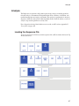
How to Load a Calibration File. . . . . . . . . . . . . . . . . . . . . . . . . . . . . . . . . . 41
Working With ROIs . . . . . . . . . . . . . . . . . . . . . . . . . . . . . . . . . . . . . . . 42
Creating ROIs With an Analysis Routine . . . . . . . . . . . . . . . . . . . . . . . . . . . 43
Loading ROIs From an ROI File . . . . . . . . . . . . . . . . . . . . . . . . . . . . . . . 45
Deleting One ROI . . . . . . . . . . . . . . . . . . . . . . . . . . . . . . . . . . . . . . . 46
Clearing All ROIs . . . . . . . . . . . . . . . . . . . . . . . . . . . . . . . . . . . . . . . 46
How to Analyze a Spectrum . . . . . . . . . . . . . . . . . . . . . . . . . . . . . . . . . . . 47
How to Select a Different Sequence File . . . . . . . . . . . . . . . . . . . . . . . . . . . 47
How to Start the Analysis . . . . . . . . . . . . . . . . . . . . . . . . . . . . . . . . . . . 48
How to Stop the Analysis . . . . . . . . . . . . . . . . . . . . . . . . . . . . . . . . . . . 49
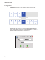
How to Use Sample Info . . . . . . . . . . . . . . . . . . . . . . . . . . . . . . . . . . . . . 50
Entering Sample Information . . . . . . . . . . . . . . . . . . . . . . . . . . . . . . . . . 50
Transferring the Spectrum . . . . . . . . . . . . . . . . . . . . . . . . . . . . . . . . . . . 51
Creating the Report in Genie 2000 . . . . . . . . . . . . . . . . . . . . . . . . . . . . . . 51
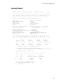
Example Report . . . . . . . . . . . . . . . . . . . . . . . . . . . . . . . . . . . . . . . . 53
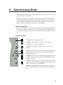
8. Spectroscopy Mode . . . . . . . . . . . . . . . . . . . . . . . . 55
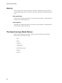
Alarms . . . . . . . . . . . . . . . . . . . . . . . . . . . . . . . . . . . . . . . . . . . . . . 56
The Spectroscopy Mode Menus . . . . . . . . . . . . . . . . . . . . . . . . . . . . . . . . . 56
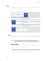
File . . . . . . . . . . . . . . . . . . . . . . . . . . . . . . . . . . . . . . . . . . . . . . . . 57
Save . . . . . . . . . . . . . . . . . . . . . . . . . . . . . . . . . . . . . . . . . . . . . . 57
iii
Open . . . . . . . . . . . . . . . . . . . . . . . . . . . . . . . . . . . . . . . . . . . . . . 58
Close . . . . . . . . . . . . . . . . . . . . . . . . . . . . . . . . . . . . . . . . . . . . . . 59
Delete . . . . . . . . . . . . . . . . . . . . . . . . . . . . . . . . . . . . . . . . . . . . . 59
MCA . . . . . . . . . . . . . . . . . . . . . . . . . . . . . . . . . . . . . . . . . . . . . . . 59
Preset Time . . . . . . . . . . . . . . . . . . . . . . . . . . . . . . . . . . . . . . . . . . 60
Preset Values . . . . . . . . . . . . . . . . . . . . . . . . . . . . . . . . . . . . . . . 60
Preset Mode . . . . . . . . . . . . . . . . . . . . . . . . . . . . . . . . . . . . . . . . 60
Hardware Settings . . . . . . . . . . . . . . . . . . . . . . . . . . . . . . . . . . . . . . . 60
Clear All . . . . . . . . . . . . . . . . . . . . . . . . . . . . . . . . . . . . . . . . . . . . 61
Stabilize . . . . . . . . . . . . . . . . . . . . . . . . . . . . . . . . . . . . . . . . . . . . 61
Using a Stabilized Probe . . . . . . . . . . . . . . . . . . . . . . . . . . . . . . . . . 62
Using the Stabilize Function . . . . . . . . . . . . . . . . . . . . . . . . . . . . . . . 63
Calibrate . . . . . . . . . . . . . . . . . . . . . . . . . . . . . . . . . . . . . . . . . . . . . 65
Energy . . . . . . . . . . . . . . . . . . . . . . . . . . . . . . . . . . . . . . . . . . . . . 65
Load . . . . . . . . . . . . . . . . . . . . . . . . . . . . . . . . . . . . . . . . . . . . 66
Recalibrating the InSpector . . . . . . . . . . . . . . . . . . . . . . . . . . . . . . . . 66
Auto Recal. . . . . . . . . . . . . . . . . . . . . . . . . . . . . . . . . . . . . . . . . 66
Manual Recal . . . . . . . . . . . . . . . . . . . . . . . . . . . . . . . . . . . . . . . 68
Show. . . . . . . . . . . . . . . . . . . . . . . . . . . . . . . . . . . . . . . . . . . . 70
Coeff. . . . . . . . . . . . . . . . . . . . . . . . . . . . . . . . . . . . . . . . . . . . 71
Full . . . . . . . . . . . . . . . . . . . . . . . . . . . . . . . . . . . . . . . . . . . . 71
Efficiency . . . . . . . . . . . . . . . . . . . . . . . . . . . . . . . . . . . . . . . . . . . 74
Load . . . . . . . . . . . . . . . . . . . . . . . . . . . . . . . . . . . . . . . . . . . . 74
Show. . . . . . . . . . . . . . . . . . . . . . . . . . . . . . . . . . . . . . . . . . . . 75
Sample Info . . . . . . . . . . . . . . . . . . . . . . . . . . . . . . . . . . . . . . . . . . . . 76
Info . . . . . . . . . . . . . . . . . . . . . . . . . . . . . . . . . . . . . . . . . . . . . . . . 77
Display . . . . . . . . . . . . . . . . . . . . . . . . . . . . . . . . . . . . . . . . . . . . . . 80
Zoom. . . . . . . . . . . . . . . . . . . . . . . . . . . . . . . . . . . . . . . . . . . . . . 80
Zoom None . . . . . . . . . . . . . . . . . . . . . . . . . . . . . . . . . . . . . . . . 81
Zoom In . . . . . . . . . . . . . . . . . . . . . . . . . . . . . . . . . . . . . . . . . . 81
Zoom Out . . . . . . . . . . . . . . . . . . . . . . . . . . . . . . . . . . . . . . . . . 81
Settings. . . . . . . . . . . . . . . . . . . . . . . . . . . . . . . . . . . . . . . . . . . . . 81
Scale . . . . . . . . . . . . . . . . . . . . . . . . . . . . . . . . . . . . . . . . . . . . 82
Borders . . . . . . . . . . . . . . . . . . . . . . . . . . . . . . . . . . . . . . . . . . 82
iv
Plot Type . . . . . . . . . . . . . . . . . . . . . . . . . . . . . . . . . . . . . . . . . 82
Gridlines . . . . . . . . . . . . . . . . . . . . . . . . . . . . . . . . . . . . . . . . . . 84
X-Units . . . . . . . . . . . . . . . . . . . . . . . . . . . . . . . . . . . . . . . . . . 84
Autoscale . . . . . . . . . . . . . . . . . . . . . . . . . . . . . . . . . . . . . . . . . 84
Max-Y . . . . . . . . . . . . . . . . . . . . . . . . . . . . . . . . . . . . . . . . . . . 84
ROI. . . . . . . . . . . . . . . . . . . . . . . . . . . . . . . . . . . . . . . . . . . . . . . 85
Delete . . . . . . . . . . . . . . . . . . . . . . . . . . . . . . . . . . . . . . . . . . . 85
Clear . . . . . . . . . . . . . . . . . . . . . . . . . . . . . . . . . . . . . . . . . . . . 86
Load . . . . . . . . . . . . . . . . . . . . . . . . . . . . . . . . . . . . . . . . . . . . 86
Analyze . . . . . . . . . . . . . . . . . . . . . . . . . . . . . . . . . . . . . . . . . . . . . . 87
Loading the Sequence File. . . . . . . . . . . . . . . . . . . . . . . . . . . . . . . . . . . 87
Starting an Analysis . . . . . . . . . . . . . . . . . . . . . . . . . . . . . . . . . . . . . . 89
Stopping an Analysis . . . . . . . . . . . . . . . . . . . . . . . . . . . . . . . . . . . . . 89
9. Setup Mode . . . . . . . . . . . . . . . . . . . . . . . . . . . . 90
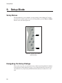
Setup Menus . . . . . . . . . . . . . . . . . . . . . . . . . . . . . . . . . . . . . . . . . . . 90
Navigating the Setup Dialogs. . . . . . . . . . . . . . . . . . . . . . . . . . . . . . . . . . . 90
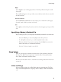
Specifying a Memory-Resident File . . . . . . . . . . . . . . . . . . . . . . . . . . . . . . 91
Dose Setup . . . . . . . . . . . . . . . . . . . . . . . . . . . . . . . . . . . . . . . . . . . . 91
Units and Range . . . . . . . . . . . . . . . . . . . . . . . . . . . . . . . . . . . . . . . . 91
Dose Rate Warning . . . . . . . . . . . . . . . . . . . . . . . . . . . . . . . . . . . . . . 92
Dose Rate Alarm. . . . . . . . . . . . . . . . . . . . . . . . . . . . . . . . . . . . . . . . 92
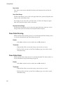
Annunciator . . . . . . . . . . . . . . . . . . . . . . . . . . . . . . . . . . . . . . . . . . 93
Cumulative Dose Warning. . . . . . . . . . . . . . . . . . . . . . . . . . . . . . . . . . . 93
Cumulative Dose Alarm . . . . . . . . . . . . . . . . . . . . . . . . . . . . . . . . . . . . 93
Neutron Count Rate Alarm . . . . . . . . . . . . . . . . . . . . . . . . . . . . . . . . . . 94
Locator Setup . . . . . . . . . . . . . . . . . . . . . . . . . . . . . . . . . . . . . . . . . . . 94
Locator . . . . . . . . . . . . . . . . . . . . . . . . . . . . . . . . . . . . . . . . . . . . . 94
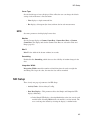
MCS . . . . . . . . . . . . . . . . . . . . . . . . . . . . . . . . . . . . . . . . . . . . . . 95
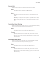
NID Setup. . . . . . . . . . . . . . . . . . . . . . . . . . . . . . . . . . . . . . . . . . . . . 95
Spec Setup . . . . . . . . . . . . . . . . . . . . . . . . . . . . . . . . . . . . . . . . . . . . 96
Peak Analysis . . . . . . . . . . . . . . . . . . . . . . . . . . . . . . . . . . . . . . . . . 96
NID Analysis . . . . . . . . . . . . . . . . . . . . . . . . . . . . . . . . . . . . . . . . . 97
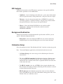
Background Subtraction . . . . . . . . . . . . . . . . . . . . . . . . . . . . . . . . . . . . 97
v
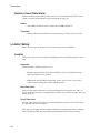
Calibration Setup . . . . . . . . . . . . . . . . . . . . . . . . . . . . . . . . . . . . . . . 97
MCA Setup . . . . . . . . . . . . . . . . . . . . . . . . . . . . . . . . . . . . . . . . . . . . 98
Instrument Setup . . . . . . . . . . . . . . . . . . . . . . . . . . . . . . . . . . . . . . . . . 98
Instrument Setup . . . . . . . . . . . . . . . . . . . . . . . . . . . . . . . . . . . . . . . . 98
Sound Setup . . . . . . . . . . . . . . . . . . . . . . . . . . . . . . . . . . . . . . . . . . 99
Date/Time Setup . . . . . . . . . . . . . . . . . . . . . . . . . . . . . . . . . . . . . . . . . 99
System Date/Time . . . . . . . . . . . . . . . . . . . . . . . . . . . . . . . . . . . . . . . 99
Time Zone . . . . . . . . . . . . . . . . . . . . . . . . . . . . . . . . . . . . . . . . . . . 99
Touchpad Calibrate . . . . . . . . . . . . . . . . . . . . . . . . . . . . . . . . . . . . . . . 100
Allow Remote Setup . . . . . . . . . . . . . . . . . . . . . . . . . . . . . . . . . . . . . . 100
Clear Cumulative Dose . . . . . . . . . . . . . . . . . . . . . . . . . . . . . . . . . . . . . 100
Reset Defaults . . . . . . . . . . . . . . . . . . . . . . . . . . . . . . . . . . . . . . . . . . 101
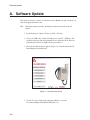
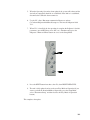
A. Software Update . . . . . . . . . . . . . . . . . . . . . . . . . 102
B. The Maintenance Utility . . . . . . . . . . . . . . . . . . . . . 104
Starting the Utility. . . . . . . . . . . . . . . . . . . . . . . . . . . . . . . . . . . . . . . . 104
The Utility’s Menu Bar . . . . . . . . . . . . . . . . . . . . . . . . . . . . . . . . . . . . . 105
File – Delete remote files . . . . . . . . . . . . . . . . . . . . . . . . . . . . . . . . . . . 105
File – Open local preference file . . . . . . . . . . . . . . . . . . . . . . . . . . . . . . . 105
Send . . . . . . . . . . . . . . . . . . . . . . . . . . . . . . . . . . . . . . . . . . . . . 105
Get . . . . . . . . . . . . . . . . . . . . . . . . . . . . . . . . . . . . . . . . . . . . . . 105
Edit . . . . . . . . . . . . . . . . . . . . . . . . . . . . . . . . . . . . . . . . . . . . . . 105
View . . . . . . . . . . . . . . . . . . . . . . . . . . . . . . . . . . . . . . . . . . . . . 106
Connect Function . . . . . . . . . . . . . . . . . . . . . . . . . . . . . . . . . . . . . . . . 106
Suppressing the ActiveSync Connection Wizard . . . . . . . . . . . . . . . . . . . . . . 107
Edit Function . . . . . . . . . . . . . . . . . . . . . . . . . . . . . . . . . . . . . . . . . . 107
Get Function. . . . . . . . . . . . . . . . . . . . . . . . . . . . . . . . . . . . . . . . . . . 107
Send Function . . . . . . . . . . . . . . . . . . . . . . . . . . . . . . . . . . . . . . . . . . 108
Viewing an InSpector Spectrum . . . . . . . . . . . . . . . . . . . . . . . . . . . . . . . 109
Sending ROI Sets . . . . . . . . . . . . . . . . . . . . . . . . . . . . . . . . . . . . . . . . 110
Defining Spectrum ROIs . . . . . . . . . . . . . . . . . . . . . . . . . . . . . . . . . . . 111
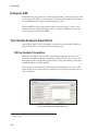
Configuration Editor . . . . . . . . . . . . . . . . . . . . . . . . . . . . . . . . . . . . . . 112
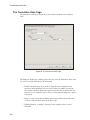
Saving the Configuration . . . . . . . . . . . . . . . . . . . . . . . . . . . . . . . . . . . 112
vi
Editing a Configuration File on Your PC . . . . . . . . . . . . . . . . . . . . . . . . . . 112
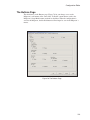
The Buttons Page . . . . . . . . . . . . . . . . . . . . . . . . . . . . . . . . . . . . . . . 113
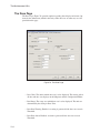
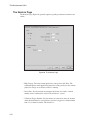
The Dose Page . . . . . . . . . . . . . . . . . . . . . . . . . . . . . . . . . . . . . . . . 114
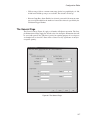
The Neutron Page . . . . . . . . . . . . . . . . . . . . . . . . . . . . . . . . . . . . . . 116
The General Page. . . . . . . . . . . . . . . . . . . . . . . . . . . . . . . . . . . . . . . 117
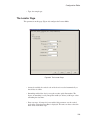
The Locator Page . . . . . . . . . . . . . . . . . . . . . . . . . . . . . . . . . . . . . . . 119
The MCA Page . . . . . . . . . . . . . . . . . . . . . . . . . . . . . . . . . . . . . . . . 121
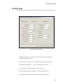
The NID Page . . . . . . . . . . . . . . . . . . . . . . . . . . . . . . . . . . . . . . . . 123
The Sound Page . . . . . . . . . . . . . . . . . . . . . . . . . . . . . . . . . . . . . . . 124
The Cumulative Dose Page. . . . . . . . . . . . . . . . . . . . . . . . . . . . . . . . . . 128
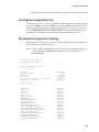
Printing the Configuration File . . . . . . . . . . . . . . . . . . . . . . . . . . . . . . . . 129
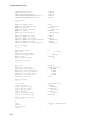
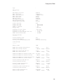
The Default Configuration Settings . . . . . . . . . . . . . . . . . . . . . . . . . . . . . 129
C. Technical Reference . . . . . . . . . . . . . . . . . . . . . . . 132
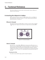
Connecting the InSpector’s Cables . . . . . . . . . . . . . . . . . . . . . . . . . . . . . . . 132
Where to Connect . . . . . . . . . . . . . . . . . . . . . . . . . . . . . . . . . . . . . . 132
How to Connect . . . . . . . . . . . . . . . . . . . . . . . . . . . . . . . . . . . . . . . 132
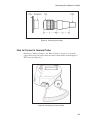
How to Connect a Gamma Probe. . . . . . . . . . . . . . . . . . . . . . . . . . . . . . . 133
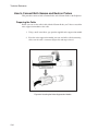
How to Connect Both Gamma and Neutron Probes . . . . . . . . . . . . . . . . . . . . . 134
Preparing the Cable . . . . . . . . . . . . . . . . . . . . . . . . . . . . . . . . . . . 134
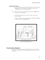
Attaching the Probes . . . . . . . . . . . . . . . . . . . . . . . . . . . . . . . . . . . 135
Cleaning the InSpector . . . . . . . . . . . . . . . . . . . . . . . . . . . . . . . . . . . . . 135
LCD Screen Protector . . . . . . . . . . . . . . . . . . . . . . . . . . . . . . . . . . . . . . 136
Setting the Hardware Gain . . . . . . . . . . . . . . . . . . . . . . . . . . . . . . . . . . . 136
Location of the GM Tube . . . . . . . . . . . . . . . . . . . . . . . . . . . . . . . . . . . . 136
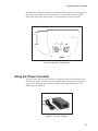
Using the Power Converter . . . . . . . . . . . . . . . . . . . . . . . . . . . . . . . . . . . 137
Intelligent Probes . . . . . . . . . . . . . . . . . . . . . . . . . . . . . . . . . . . . . . . . 138
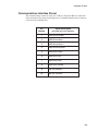
Communications Interface Pinout . . . . . . . . . . . . . . . . . . . . . . . . . . . . . . 139
Probe Connector Pinout . . . . . . . . . . . . . . . . . . . . . . . . . . . . . . . . . . . 140
Probe Format Data File . . . . . . . . . . . . . . . . . . . . . . . . . . . . . . . . . . . . . 141
Probe HV Cutoff Level Adjustment. . . . . . . . . . . . . . . . . . . . . . . . . . . . . . . 142
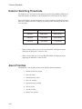
Detector Switching Thresholds . . . . . . . . . . . . . . . . . . . . . . . . . . . . . . . . . 144
Alarm Priorities . . . . . . . . . . . . . . . . . . . . . . . . . . . . . . . . . . . . . . . . . 144
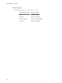
Efficiency Calibration Models . . . . . . . . . . . . . . . . . . . . . . . . . . . . . . . . . 145
vii
Default InSpector Files . . . . . . . . . . . . . . . . . . . . . . . . . . . . . . . . . . . . . 145
Input Power Requirements . . . . . . . . . . . . . . . . . . . . . . . . . . . . . . . . . . . 146
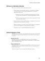
The Internal Battery . . . . . . . . . . . . . . . . . . . . . . . . . . . . . . . . . . . . . 146
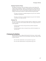
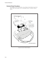
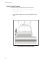
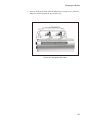
Changing the Battery . . . . . . . . . . . . . . . . . . . . . . . . . . . . . . . . . . . . . . 147
Gamma Probe Procedure . . . . . . . . . . . . . . . . . . . . . . . . . . . . . . . . . . . 148
Neutron Probe Procedure . . . . . . . . . . . . . . . . . . . . . . . . . . . . . . . . . . . 150
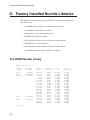
D. Factory Installed Nuclide Libraries . . . . . . . . . . . . . . . 154
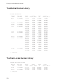
The NORM Nuclear Library . . . . . . . . . . . . . . . . . . . . . . . . . . . . . . . . . . 154
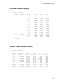
The SNM Nuclear Library . . . . . . . . . . . . . . . . . . . . . . . . . . . . . . . . . . . 155
The NaI Demo Nuclear Library . . . . . . . . . . . . . . . . . . . . . . . . . . . . . . . . . 155
The Medical Nuclear Library . . . . . . . . . . . . . . . . . . . . . . . . . . . . . . . . . . 156
The Peak Locate Nuclear Library . . . . . . . . . . . . . . . . . . . . . . . . . . . . . . . . 156
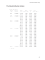
The Industrial Nuclear Library . . . . . . . . . . . . . . . . . . . . . . . . . . . . . . . . . 157
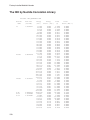
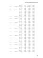
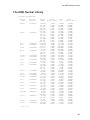
The NID by Nuclide Correlation Library . . . . . . . . . . . . . . . . . . . . . . . . . . . . 158
The ANSI Nuclear Library . . . . . . . . . . . . . . . . . . . . . . . . . . . . . . . . . . . 161
E. Using ASFs . . . . . . . . . . . . . . . . . . . . . . . . . . . . 162
Creating or Editing an ASF . . . . . . . . . . . . . . . . . . . . . . . . . . . . . . . . . . . 162
Using an ASF . . . . . . . . . . . . . . . . . . . . . . . . . . . . . . . . . . . . . . . . . . 164
Two Useful Analysis Algorithms . . . . . . . . . . . . . . . . . . . . . . . . . . . . . . . . 164
NID by Nuclide Correlation . . . . . . . . . . . . . . . . . . . . . . . . . . . . . . . . . 164
Dose by Isotope . . . . . . . . . . . . . . . . . . . . . . . . . . . . . . . . . . . . . . . 165
F. Specifications . . . . . . . . . . . . . . . . . . . . . . . . . . 166
Physical . . . . . . . . . . . . . . . . . . . . . . . . . . . . . . . . . . . . . . . . . . . . . 166
Environmental . . . . . . . . . . . . . . . . . . . . . . . . . . . . . . . . . . . . . . . . . . 166
Inputs . . . . . . . . . . . . . . . . . . . . . . . . . . . . . . . . . . . . . . . . . . . . . . 166
Outputs . . . . . . . . . . . . . . . . . . . . . . . . . . . . . . . . . . . . . . . . . . . . . 166
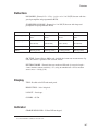
Detectors . . . . . . . . . . . . . . . . . . . . . . . . . . . . . . . . . . . . . . . . . . . . 167
Display . . . . . . . . . . . . . . . . . . . . . . . . . . . . . . . . . . . . . . . . . . . . . 167
Indicator . . . . . . . . . . . . . . . . . . . . . . . . . . . . . . . . . . . . . . . . . . . . . 167
Beeper . . . . . . . . . . . . . . . . . . . . . . . . . . . . . . . . . . . . . . . . . . . . . . 168
Count/Dose Rate Display . . . . . . . . . . . . . . . . . . . . . . . . . . . . . . . . . . . . 168
viii
Battery . . . . . . . . . . . . . . . . . . . . . . . . . . . . . . . . . . . . . . . . . . . . . . 168
Performance . . . . . . . . . . . . . . . . . . . . . . . . . . . . . . . . . . . . . . . . . . . 168
Index . . . . . . . . . . . . . . . . . . . . . . . . . . . . . . . . . 171
ix
Preface
The InSpector™ 1000 is an easy-to-use digital handheld multichannel analyzer, ideally suited
for:
• Homeland Security and First
Responder Applications (fire fighters,
law enforcement, Coast Guard,
hospital emergency personnel).
• Customs and Border Controls.
• Waste (scrap) Applications.
• Health Physics Applications which
need isotope specific results.
• In Situ Environmental Screening.
• Treaty and Non-proliferation
Compliance.
• Monitoring of Nuclear
Transportation.
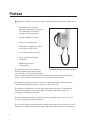
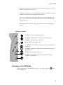
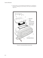
The InSpector 1000 and Attached Probe
The InSpector 1000 can be used for any
field measurement application requiring
dose and count rate measurements, locating
sources, nuclide identification with activity measurements, and spectrum acquisition and
analysis. All these modes of operations are easily selectable with one touch.
The InSpector 1000 gives results not just data! It continuously updates information about
radiation hazards: identified nuclides, nuclide activities or dose rate.
The InSpector 1000 provides a flexible application-specific response by accommodating
different detector/probe sizes and technologies. The high voltage power supply and
preamplifier are built into each probe.
The instrument automatically recognizes each of these intelligent probes and it selects the
associated calibrations and other parameters.
The crisp color display and well-organized six hard buttons allow the user quick access to all
modes and to switch from one mode to another with one push of a button! Even with gloved
x
hands, the user can also use the touch screen instead of these hard keys. The intuitive user
interface provides the ultimate flexibility in field operations.
InSpector 1000 is readily usable without the need of extensive training and also offers
high-level spectrometry analysis capabilities for expert use.
One-click simplicity masks the powerful spectral processing built within this instrument. This
instrument provides a level of performance previously available only in sophisticated
computer-based laboratory systems. It offers the full power of Canberra’s time-tested spectrum
processing algorithms – minimizing false positive identifications while improving sensitivity
for low level shielded and mixed sources, or sources “hidden” by natural or legitimate
radioactive materials.
Moreover, the use of Digital Signal Processing technology improves the overall signal
acquisition performance; this results in increased stability, accuracy, consistency and
reproducibility in a Smart probe instrument.
xi
Notes
xii
1. Introduction
The InSpector™ 1000’s software runs under the Windows® CE operating system.
Though it may seem that other Windows CE applications could be run on the InSpector, doing so will cause undesirable results and may void your warranty.
CAUTION • Do not use the InSpector as a PDA.
• Do not use the InSpector to run other Windows CE
applications.
Doing so will cause the InSpector to malfunction and may
cause data to be corrupted or irretrievably lost.
About This Manual
The InSpector 1000 User’s Manual is designed for users of all levels of sophistication.
Each chapter is a tutorial, addresses an operating mode or explains how to set up the
instrument for daily operation.
Chapter 2, Quick Start, uses the Dose Mode as a brief introduction to working with
the InSpector’s Dose, Locator and Nuclide ID operating modes.
Chapter 4, Dose Mode, presents a quick view of both the Instantaneous Dose Rate and
the Cumulative Dose in one of several different display modes in your choice of
sievert, roentgen or rem units.
Chapter 5, Locator Mode, charts the moment by moment radiation intensity seen by
the InSpector, helping you locate lost, hidden or contraband sources of radiation.
Chapter 6, Nuclide ID Mode, provides continuous real-time identification of individual isotopes with their activity calculation, in either Bq or µCi.
Chapter 7, Spectroscopy Tutorials, is based on Genie 2000’s gamma analysis functions. This chapter explains how the InSpector implements those functions.
Chapter 8, Spectroscopy Mode, lets you collect and analyze radionuclide spectra with
the spectroscopy tools normally found only in a high-end MCA.
Chapter 9, Setup Mode, lets you set the system-wide parameters and the parameters
for each of the four data modes.
Quick Start
2. Quick Start
The Quick Start chapter uses the Dose Mode as a brief introduction to working with
the InSpector’s Dose, Locator and Nuclide ID operating modes. The Spectroscopy
mode has its own tutorial, starting on page 29.
Preparing the InSpector
If you haven’t already connected the probe(s) to your InSpector, refer to “Connecting
the InSpector’s Cables” on page 132 for instructions.
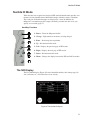
Turning on the InSpector™
To turn on the InSpector,
select the Power key
(Figure 1).
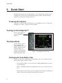
The Dose Mode
The Dose Mode, which is
always running in the
background, measures and
displays both the instantaneous Dose Rate, the
amount of radiation being
measured at this moment,
and the Cumulative Dose.
Figure 1 The InSpector's Front Panel
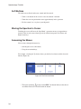
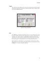
Displaying the Dose Mode’s Data
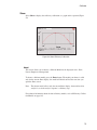
There are several ways of displaying the Dose Mode’s data. As an example, the Simple Dose Rate display in Figure 2 shows:
• The current Dose Rate as a value and unit, 1.8 mR/h (milliRoentgens per hour)
as a histogram bar.
• The bar’s highlighted length is the proportion of the value, 1.8, to the full scale,
10.0.
• The histogram’s first (yellow) vertical bar indicates the Dose Rate warning level
and the second (red) bar indicates the Dose Rate alarm level.
2
The Status Line
Figure 2 The Simple Dose Display
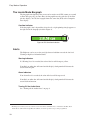
The Status Line
The Status Line at the bottom of the screen (Figure 3) displays several status indicators:
Figure 3 The Status Bar
• The current instrument status: Idle, Acquiring, High Field, Stabilized, Hold,
No Probe or ERROR.
• The current analysis status: Analyzing or ERROR.
• The audio icons disable/enable an active Annunciator or Alarm/Warning audio
output.
u
The Annunciator output is active only if the Annunciator (page 19) has
been enabled. Selecting the audio icons
will turn the
Annunciator audio off and put a red X through the Annunciator icon.
3
Quick Start
u
If any enabled Warning or Alarm threshold is exceeded (page 91), its
audio alert will be heard.
Turning Off the Audio Alerts
u Selecting the audio icons a second time will turn the Alarms audio off
and put a red X through the Alarms icon.
u
Select the icons again to re-enable the first audio output, and a second
time to re-enable the second audio output.
u
If the Annunciator has not been enabled, its icon will always be disabled.
In this case, only the Alarms icon can be toggled between on and off.
shows that the InSpector is using an
• There are two power icons: One
external power source; the other shows that the internal battery
is
powering the unit, and shows the battery charge remaining.
• A Help icon.
Select this button to display the help screen for the current
Mode or dialog screen.
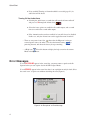
Error Messages
If a red NO PROBE appears in the status line, you must connect a probe to the InSpector before you can acquire data in the NID or Spec Modes.
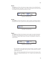
If a red ERROR appears in the status line, there is an acquisition or analysis fault. Select
the word “error” to open a text window describing the error (Figure 4).
Figure 4 An Example of an Error Message
4
Navigating the InSpector’s Menus
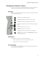
Navigating the InSpector’s Menus
There are two ways to navigate around the InSpector 1000’s menus and functions: by
the hard keys to the left of the display or by the soft buttons on the display.
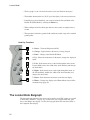
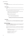
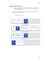
Hard Keys
These are general descriptions of the hard keys’ functions. The function of most keys
depends on which mode is active.
1. Power: Cycles the InSpector On/Off.
2. Charge: Light whenever the battery is being charged.
3. Enter: Function varies, depending on the active mode.
4. Up: Enters the main menu; in the menu, changes the displayed
mode.
5. Left: In the menu, moves to the left.
6. Right: In the menu, moves to the right.
7. Down: Exits the menu and returns to the current display.
8. Home: Changes the display to the Home Mode selected in Instrument Setup (page 98).
Soft Buttons
The touchscreen allows both coarse control and fine control.
• Touch a soft button on the screen to select that button’s function.
• For fine control, use a stylus or your fingernail.
The Home Mode
You can always select the Home button to go back to the default operating mode, as
defined in Instrument Setup (page 98).
5
Quick Start
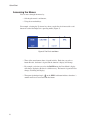
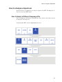
Accessing the Menus
You can move through the menus by:
• Selecting the menu’s soft buttons,
• Using the arrow hardkeys.
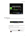
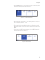
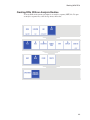
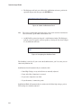
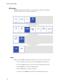
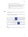
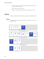
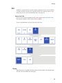
For example, selecting the Up Arrow key shows you the first level menu with a soft
button for each of the InSpector’s operating modes (Figure 5).
Figure 5 The First Level Menu
• Three of the menu buttons show a legend in italics. Each time you select a
button like this, the button’s legend and the function’s display will change.
• For example, each time you select the DOSE button, the Dose Mode’s display
will change, displaying the data in a different way. The button’s legend will also
change, describing that display.
• The upward pointing triangle
on the SPEC soft button indicates that there’s
another menu level associated with that button.
6
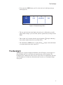
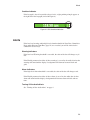
The Backlight
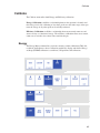
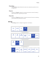
• If you select the SPEC button, you’ll see the next level of the Spectroscopy
menu (Figure 6).
Figure 6 The Spectroscopy Menu
• The area just below the menu displays the path you’ve followed to get to this
point. In this example, you can see that you have gotten here by having selected
SPEC.
• Three of this level’s buttons show the upward-pointing
that each has another menu level associated with it.
• The fourth button, NEXT, shows a right-pointing
to see more menu items at the same level.
triangle, indicating
triangle. Select this button
The Backlight
The InSpector’s display backlight will illuminate the LCD display in low light or no
light conditions but its use will reduce the operating time of the instrument. The
backlight can be configured to always be On, always Off, or to automatically turn off a
specified number of seconds after the unit becomes inactive (see “Instrument Setup”
on page 98).
7
Easy Mode of Operation
3. Easy Mode of Operation
The InSpector is normally set for this mode of operation. If your unit is set to the Standard Mode, you’ll find the information you need in the chapters on Dose Mode, Locator Mode, NID Mode and Spectroscopy Mode.
There are two main functions in the Easy Mode:
• The Locator (LOC) function, which lets you locate the source of radioactivity,
making it easy to locate lost, hidden or contraband sources (this page).
• The Nuclide Identifier (NID) function, which identifies individual isotopes and
their activity (page 11).
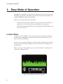
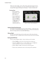
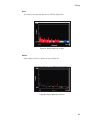
Locator Mode
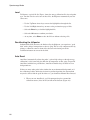
As soon as the Locator Mode is selected, it begins operating, displaying a histogram.
The Dose Rate is continuously evaluated and the warning and alarm levels are constantly tracked by the InSpector.
As you scan an area with the InSpector’s probe, the change in intensity lets you locate
the source of the radioactivity, making it easy to precisely locate lost, hidden or contraband sources.
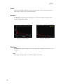
When you select the Locator Mode, you’ll see a bar chart (Figure 7) showing the instantaneous radiation intensity.
Figure 7 Locator Mode, in Counts per Second
8
Locator Mode
• The most current data (i.e., time now) is the right end of the display. As time
advances, data will move to the left.
• In Figure 7, the display’s x-axis is calibrated in counts. The width of the graph,
in time, is the figure below the right end of the graph.
• The y-axis is calibrated in CPS or Dose Rate units (selected in Monitor, page
95); its range can be changed and Autoscale can be enabled (both selected in
Locator, page 94).
• When configured for Dose Rate operation, the dose results are updated once a
second.
Hard Key Functions
1. Power – Turns the InSpector On/Off.
2. Charge – Light whenever the battery is being charged.
3. Enter – Starts/stops data acquisition.
4. Up – No function in this mode.
5. Left – Halves the width of the dwell window (and changes the
dwell time).
6. Right – Doubles the width of the dwell window (and changes
the dwell time).
7. Down – No function in this mode.
8. Home – Changes the display back and forth between the
LOCate and NID modes.
Changing to the NID Mode
To change the display to the NID Mode (page 11), select the isotope icon
keypad’s Home key.
or the
9
Easy Mode of Operation
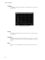
The Locate Mode Bargraph
The bargraph at the bottom of the screen can be made to read CPS (counts per second)
or Dose Rate (page 95). As Dose Rate, the bargraph shows the same data as the Simple dose display. As CPS, the bargraph shows the same data (ICR) as the Composite
dose display.
Overflow Indicator
If the bargraph’s data is beyond the selected scale, a right-pointing triangle appears at
the right end of the bargraph (circled in Figure 8).
Figure 8 CPS Overflow Indication
Alerts
The InSpector can be set to alert you if the detected radiation exceeds the low level
Warning or high level Alarm threshold. *
Warning Indicators
If a Warning Level is exceeded, the color of the bar will change to yellow.
If enabled, an audio alert will sound and the display's background will alternate between black and gold.
Alarm Indicators
If an Alarm Level is exceeded, the color of the bar will change to red.
If enabled, an audio alert will sound and the display's background will alternate between black and maroon.
Turning Off the Audio Alerts
See “Turning off the Audio Alerts” on page 4.
*The InSpector can alert you to any or all of excessive Dose Rate, Cumulative Dose or Neutron Count Rate. Their
thresholds are defined in the Setup Mode. In addition, an alert for specific isotopes can be programmed.
10
Nuclide ID Mode
Nuclide ID Mode
When data has been acquired and analyzed, NID (nuclide identification) provides continuous real-time identification of individual isotopes with their activity calculation.
The results for all identified isotopes are displayed as a chart. In addition, the
InSpector™ can monitor specific isotopes and notify you when the alert levels you
specify are exceeded (page 27).
Hard Key Functions
1. Power – Turns the InSpector On/Off.
2. Charge – Light whenever the battery is being charged.
3. Enter – Starts/stops data acquisition.
4. Up – No function in this mode.
5. Left – Displays the previous page of NID results.
6. Right – Displays the next page of NID results.
7. Down – No function in this mode.
8. Home – Changes the display between the NID and LOCate modes.
The NID Display
The Easy Mode display (Figure 9) lists the identified nuclides, their isotope type (fission, activation, etc.), and either dose rate or activity.
Figure 9 The Nuclide ID Display
11
Easy Mode of Operation
Changing to the Locator Mode
To change the display to the Locator Mode (page 8), select the onscreen Locate button
or the keypad’s Home key.
Calibrating the InSpector
Select the onscreen Calibrate button
to access the InSpector’s standard Auto Recal
function, which is covered in detail starting on page 66.
Note: The CAL button will be not be seen when data acquisition is in process.
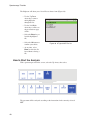
Starting Data Acquisition
To acquire nuclide data, select the Enter key.
• If there already is a list of nuclide data, you’ll be asked if you want to start a
New acquisition or Resume the old one.
• When data acquisition terminates, the identified nuclides will be listed in the
nuclide table.
• If more nuclides have been found than can be listed on the page, use the
right/left arrow keys to move between pages.
Selecting Which NID Data to Display
• Selecting the first column’s heading orders the column by atomic mass.
• Selecting the last column’s heading toggles the data between activity and dose
rate.
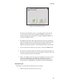
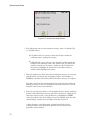
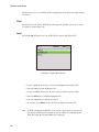
Saving the Data
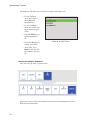
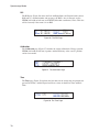
When acquisition is off, select the keyboard’s Enter key to start a New data acquisition, with or without Saving the current data (Figure 10).
Note: Data cannot be saved when data acquisition is in process.
12
Nuclide ID Mode
Figure 10 Saving the Data
• New clears the data and starts a new acquisition.
• Save/New saves the current data before starting a new acquisition.
Isotope-Specific Alerts
The InSpector can announce warnings and alerts for specific nuclides. This feature is
set up in the Standard Operating Mode (page 27).
If the Nuclide’s Warning Level is Exceeded
• The General Alert Warning Indicator (described below) is triggered.
• The nuclide’s line will blink yellow.
If the Nuclide’s Alarm Level is Exceeded
• The General Alert Alarm Indicator (described below) is triggered.
• The nuclide’s line will blink red.
General Alerts
The InSpector can be set to alert you if the detected radiation exceeds the low level
Warning or high level Alarm threshold. *
Warning Indicators
If a Warning Level is exceeded, the color of the bar will change to yellow.
If enabled, an audio alert will sound and the display's background will alternate between black and gold.
*In addition to the alert for specific isotopes, the InSpector can alert you to any or all of excessive Dose Rate,
Cumulative Dose or Neutron Count Rate. Their Warning and Alarm thresholds are defined in the Setup Mode.
13
Easy Mode of Operation
Alarm Indicators
If an Alarm Level is exceeded, the color of the bar will change to red.
If enabled, an audio alert will sound and the display's background will alternate between black and maroon.
Turning Off the Audio Alerts
See “Turning off the Audio Alerts” on page 4.
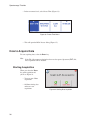
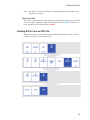
Using a Stabilized Probe
The Stabilized Probe is very easy to use. When the InSpector finds a Stabilized Probe
connected to its DET connector, it will display a message for about 30 seconds, advising you that the probe is stabilizing (Figure 11).
Figure 11 The Probe is Stabilizing
• The blue LED on the probe will blink while stabilization is in process. When
stabilization is complete, the LED will glow steadily.
• If stabilization is lost, perhaps due to moving the unit from a warm environment
to a cold one (indoors to outdoors), data acquisition will stop and the instrument
will restabilize itself (the blue LED will start blinking). When the LED glows
steadily, stabilization is complete and acquisition can be restarted.
14
Using a Stabilized Probe
• If you enter a high radiation area, High Field will be displayed at the bottom of
the screen, data acquisition will stop, the probe’s high voltage and its blue LED
will be turned off. When you leave the High Field area, the high voltage will be
turned on again and the LED will start blinking as the probe begins stabilizing.
When the LED glows steadily, stabilization is complete and acquisition can be
restarted.
15
Dose Mode
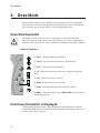
4. Dose Mode
The Dose Mode, which is always running in the background, measures and displays
the instantaneous Dose Rate, the amount of radiation being measured at this moment.
You can choose any of several displays, each providing different data.
Dose Rate Equivalent
The InSpector 1000 reports the dose rate equivalent on 10 mm of human tissue
[H*(10)]. It does not report surface tissue dose. Therefore, the values reported by the
InSpector will not be the same as those reported by instruments using surface methods.
Hard Key Functions
1. Power – Turns the InSpector™ On/Off.
2. Charge – Light whenever the battery is being charged.
3. Enter – Change to the Locator Mode.
4. Up – Enters the main menu; in the menu, changes the displayed
mode.
5. Left – In the menu, moves to the left.
6. Right – In the menu, moves to the right.
7. Down – Exits the menu and returns to the Dose display.
8. Home – Changes the display to the Home Mode selected in Instrument Setup (page 98).
How Dose Information is Displayed
All Dose Mode displays include a digital readout and visual indicators for both the
warning threshold and the alarm threshold. The thresholds and the display units are selected in “Dose Setup” (page 91).
16
How Dose Information is Displayed
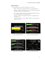
NaI Probe Displays
If a Gamma (NaI) Probe is connected to the InSpector, you can choose:
• Simple – Displays the current Gamma Dose Rate as a bargraph (Figure 12).
• Composite – Displays the Gamma Dose Rate, the Cumulative Gamma Dose and
the Gamma Count Rate as bargraphs (Figure 13).
• Ebar – Displays the Gamma Dose Rate, the Cumulative Gamma Dose and the
Average Spectrum Energy as bargraphs (Figure 14).
• Log Dial – Displays the current Gamma Dose Rate on a logarithmic analog
scale (Figure 15).
• Linear Dial – Displays the current Gamma Dose Rate on a linear analog scale
(similar to Figure 15).
Figure 12 Simple Dose Display
Figure 13 Composite Dose Display
Figure 14 Ebar Dose Display
Figure 15 Log Dial Dose Display
17
Dose Mode
Neutron Probe Displays
If a Neutron Probe is connected to the InSpector, two more displays are available.
• Dose Neutron – Displays the current Gamma Dose Rate and the Neutron Count
Rate as bargraphs (Figure 16).
• Composite Neutron – Displays the current Gamma Dose Rate, the Cumulative
Gamma Dose and the Neutron Count Rate as bargraphs (Figure 17).
Figure 16 Dose Neutron Display
Figure 17 Composite Neutron Display
Dose Alerts
If the low-level warning and/or high-level alarm thresholds for Dose Rate, Cumulative
Dose and/or Neutron Count Rate (page 91) are exceeded, you will be alerted to the
condition in several ways.
Warning Indicators
If the Warning threshold is exceeded, the color of the bar will change to yellow.
If the Enable parameter for either of these warnings is set to On, the audio alert for that
warning will sound and the display's background will alternate between black and
gold.
Alarm Indicators
If the Alarm threshold is exceeded, the color of the bar will change to red.
If the Enable parameter for either of these alarms is set to On, the audio alert for that
alarm will sound and the display's background will alternate between black and maroon.
18
Neutron Count Rate Alert
Turning Off the Audio Alerts
See “Turning off the Audio Alerts” on page 4.
Overflow Indicator
If the bargraph’s data is beyond the selected scale, a right-pointing triangle appears at
the right end of the bargraph (circled in Figure 18).
Figure 18 Dose Rate Overflow Indication
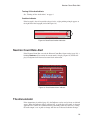
Neutron Count Rate Alert
If the Neutron Count Rate exceeds the Neutron Count Rate Alarm setting (page 94), a
blinking Neutron will overwrite the current mode’s display (Figure 19) and the display's background will alternate between black and maroon.
Figure 19 Dose Neutron Alarm Indicator
The Annunciator
If the Annunciator is enabled (page 93), the InSpector can be used to locate an isolated
source. When the InSpector detects radioactivity, an audio alert will sound. As the unit
approaches the source, the radiation intensity (incoming count rate) increases, causing
the audio output’s rate or pitch to change with the rate of detected radiation changes.
19
Dose Mode
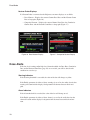
Clearing the Cumulative Dose
The Cumulative Dose is the total radiation dose received by the unit since the InSpector was turned on or since the dose memory was cleared using the Setup Mode’s Clear
Cumulative Dose command (page 100).
Changing to the NID Mode
If NID results are available (page 24), you’ll see an isotope icon
in the upper right
corner of the Dial displays. You can change from a Dial display to the NID Mode display by selecting this icon.
The Isotope Icon
If isotope-specific alerts have been enabled in the NID Mode (page 27), the isotope
icon will change to yellow if any specified isotope’s warning threshold has been exceeded or red if its alarm threshold has been exceeded.
20
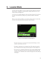
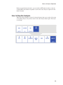
5. Locator Mode
As soon as the Locator Mode is selected, it begins operating, displaying a histogram.
The Dose Rate is continuously evaluated and the warning and alarm levels are constantly tracked by the InSpector™.
As you scan an area with the InSpector’s probe, the change in intensity lets you locate
the source of the radioactivity, making it easy to find lost, hidden or contraband
sources.
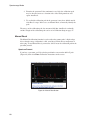
When you select the Locator Mode, you can choose to display either a bar chart (Figure 20) or a line chart showing the instantaneous radiation intensity.
Figure 20 Locator Mode with the Dose Rate Bar
• The most current data (i.e., time now) is the right end of the display. As time
advances, data will move to the left.
• The display’s horizontal axis is calibrated in time. The width of the graph, in
time, is the figure below the right end of the graph (10 seconds in Figure 20).
• The vertical axis is calibrated in CPS or Dose units (selected in Monitor Setup).
Its range can be changed or Autoscale can be enabled (in Locator Setup). The
vertical axis scale’s maximum value is shown in the upper left corner (1000 cps
in the figure).
21
Locator Mode
• The bar graph’s scale is shown below the bar (0.0 and 100.0 in the figure).
• The number shown on the bar (76.87 cps in the figure) is the current count rate.
• If nuclides have been identified, you can move from the Locator Mode to the
Nuclide ID (NID) Mode by selecting the Enter key.
• When configured for Dose Rate operation, the dose results are updated once a
second.
• The operation is limited to gamma fields within the usable range of the attached
gamma probe.
Hard Key Functions
1. Power – Turns the InSpector On/Off.
2. Charge – Light whenever the battery is being charged.
3. Enter – Change to the Nuclide ID Mode.
4. Up – Enters the main menu; in the menu, changes the displayed
mode.
5. Left – In the menu, moves to the left through the menu; in the
Locator Mode, halves the width of the dwell window (and changes
the dwell time).
6. Right – In the menu, moves to the right through the menu; in
the Locator Mode, doubles the width of the dwell window (and
changes the dwell time).
7. Down – Exits the menu and returns to the Locator display.
8. Home – Changes the display to the Home Mode selected in Instrument Setup (page 98).
The Locate Mode Bargraph
The bargraph at the bottom of the screen can be made to read CPS (counts per second)
or Dose Rate (“Monitor”, on page 95). As Dose Rate, the bargraph shows the same
data as the Simple dose display. As CPS, the bargraph shows the same data (ICR) as
the Composite dose display.
22
Alerts
Overflow Indicator
If the bargraph’s data is beyond the selected scale, a right-pointing triangle appears at
the right end of the bargraph (circled in Figure 8).
Figure 21 CPS Overflow Indication
Alerts
If the low-level warning and/or high-level alarm thresholds for Dose Rate, Cumulative
Dose and/or Neutron Count Rate (page 91) are exceeded, you will be alerted to the
condition in several ways.
Warning Indicators
If the low-level Warning threshold is exceeded, the color of the bar will change to yellow.
If the Enable parameter for either of these warnings is set to On, the audio alert for that
warning will sound and the display's background will alternate between black and
gold.
Alarm Indicators
If the high-level Alarm threshold is exceeded, the color of the bar will change to red.
If the Enable parameter for either of these alarms is set to On, the audio alert for that
alarm will sound and the display's background will alternate between black and maroon.
Turning Off the Audio Alerts
See “Turning off the Audio Alerts” on page 4.
23
Nuclide ID Mode
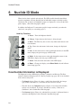
6. Nuclide ID Mode
When data has been acquired and analyzed, The NID (nuclide identification) Mode
provides continuous real-time identification of individual isotopes with their activity
calculation. The results for all identified isotopes are displayed as a chart. In the Composite display, a Dose Rate bargraph is added.
In addition, the InSpector™ can monitor specific isotopes and notify you when the
alert levels you specify are exceeded (page 27).
Hard Key Functions
1. Power – Turns the InSpector On/Off.
2. Charge – Light whenever the battery is being charged.
3. Enter – The Enter key has several easily understood context-sensitive functions.
4. Up – Enters the main menu; in the menu, changes the displayed
mode.
5. Left – In the menu, moves to the left through the menu; in the NID
mode, displays the previous page of NID results.
6. Right – In the menu, moves to the right through the menu; in the
NID mode, displays the next page of NID results.
7. Down – Exits the menu and returns to the NID display.
8. Home – Changes the display to the Home Mode selected in Instrument Setup (page 98).
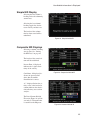
How Nuclide Information is Displayed
The InSpector has three NID displays, Simple, Composite and Neutron. The Dose
(units/h) column will display zeros if a Dose by Isotope step (page 165) is not included
in the current analysis file.
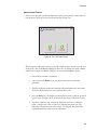
• The Simple display (Figure 22) shows a table listing the nuclide, the isotope
type (fission, activation, etc.), and either its dose rate or its activity.
• The table in the two Composite displays (Figures 23 and 24) list the Nuclide,
its dose rate (if enabled), its activity, and either its activity % Error or its
Confidence, and a Gamma Dose Rate bargraph.
• The Neutron display (Figure 24), which will be seen only if a Neutron Probe is
attached to the InSpector, adds a Neutron Count Rate bargraph.
24
How Nuclide Information is Displayed
Simple NID Display
Selecting the first column’s
heading orders the column by
atomic mass.
Selecting the last column’s
heading toggles the data between activity and dose rate.
The header of the column
that has been sorted will be
underlined.
Figure 22 Simple Nuclide ID
Composite NID Displays
Selecting a column’s heading
sorts its data. See “Sorting
the NID Data” on page 26.
The header of the sorted column will be underlined.
Percent Error, if displayed,
indicates the 1 sigma uncertainty of the activity.
Confidence, if displayed, indicates the percent confidence that the nuclide
identification is correct.
Figure 23 Composite Nuclide ID
A '*' displayed before the activity value at the head of its
column indicates that the default efficiency was used for
analysis.
The Dose Neutron Nuclide
ID screen (Figure 24) will be
seen only if a Neutron Probe
is attached to the InSpector.
Figure 24 Neutron Nuclide ID
25
Nuclide ID Mode
When two or more nuclides, such as 85Kr and 85Sr, produce their single peak at the
same energy level, the InSpector is not able to determine which nuclide to assign to
that peak. If this happens, the InSpector will display a '?' before the nuclide name.
Pressing Enter
• If data acquisition is
not in progress, “Press
Enter to start a new
NID” (Figure 22).
• If data acquisition is in
progress, “Press Enter
to Save the Spectrum”,
then select “NEW” to
acquire a new spectrum
or “RESUME” to
continue the current
acquisition (Figure 25).
Figure 25 New or Resumed Spectrum
Gamma Dose Rate Bargraph
The Gamma Dose Rate bargraph below the Composite Display’s nuclide table shows
the same data as the Simple Dose Mode display (page 17). Click on the Gamma Dose
Rate bar to change to the last selected Dose Mode display.
Library Used
The name of the nuclide library used for nuclide analysis will be shown below the
bargraph only if there is an NID step in the analysis file and a library has been defined.
Sorting the NID Data
You can sort the Composite display’s data by selecting any of its columns.
• Click on Nuclide to sort the rows in increasing order of atomic mass.
• Click on the unit/h (Dose Rate, if enabled), unit (activity) or Conf(%) (if
enabled) column title to sort the rows in decreasing order.
• Click on % Err, if enabled, to sort the rows in increasing order.
• The title of the column that has been used for sorting will be underlined.
26
How Nuclide Information is Displayed
Isotope-Specific Alerts
Genie 2000’s Nuclide Library Editor, described in its own chapter in the Genie 2000
Operations Manual, is used to set isotope-specific alerts (Action Levels) for specific
nuclides in a nuclide library (NLB) file.
• Set Action Level 1 for a nuclide to enable its warning level.
• Set Action Level 2 for a nuclide to enable its alarm level.
After modifying the nuclide library…
• Use the Maintenance Utility’s Send function (page 108) to transfer the library to
the InSpector.
• Then load it in the NID Analysis Setup (page 97).
• This library will be used for the NID Analysis step of the currently loaded
analysis sequence file.
• How to Analyze a Spectrum on page 47 tells you how to Load and Start an
analysis sequence.
After each execution of the analysis sequence, the InSpector evaluates the NID results
data, comparing the mean activity for each nuclide to the Action Level 1 and Action
Level 2 settings for that nuclide.
If the Nuclide’s Warning Level is Exceeded
• The nuclide activity Warning Indicator (described in General Alerts, below) is
triggered.
• Its line will blink yellow.
• The isotope icon
in the upper right corner the Dose Mode’s Linear Dial or
Log Dial display (page 17) will change to yellow.
If the Nuclide’s Alarm Level is Exceeded
• The nuclide activity Alarm Indicator (described in General Alerts, below) is
triggered.
• Its line will blink red.
• The isotope icon
in the upper right corner the Dose Mode’s Linear Dial or
Log Dial display (page 17) will change to red.
General Alerts
If, in addition to the Isotope-Specific Alerts, the low-level warning and/or high-level
alarm thresholds for Dose Rate, Cumulative Dose and/or Neutron Count Rate (page
91) are exceeded, you will be alerted to the condition in several ways.
27
Nuclide ID Mode
Warning Indicators
If the low-level Warning threshold is exceeded, the color of the bar will change to yellow.
If the Enable parameter for either of these warnings is set to On, the audio alert for that
warning will sound and the display's background will alternate between black and
gold.
Alarm Indicators
If the high-level Alarm threshold is exceeded, the color of the bar will change to red.
If the Enable parameter for either of these alarms is set to On, the audio alert for that
alarm will sound and the display's background will alternate between black and maroon.
Turning Off the Audio Alerts
See “Turning off the Audio Alerts” on page 4.
28
7. Spectroscopy Tutorials
This chapter describes the Spectroscopy Mode display and is a quick overview of
some of the Mode’s functions. See Chapter 8, Spectroscopy Mode, for more information.
Relationship of the InSpector™ to Genie 2000
The Spectroscopy Mode’s functions parallel the same functions in the Genie 2000
Spectroscopy Software. For detailed information, please refer to the Genie 2000 Operations Manual and the Genie 2000 Customization Tools Manual. Both are included as
PDF files on your Genie 2000 CD-ROM.
Spectral Data Conventions
Canberra’s MCAs manage two types of spectra: data currently being acquired (a “live”
spectrum) and data loaded from a file (a saved spectrum acquired at an earlier time).
Any spectroscopy function affecting the data of one type will not affect the data of the
other type.
Memory Resident Files
Several of the Spectroscopy Mode’s functions require choosing a file resident in the
InSpector’s memory as the current file, the one to be used for that function. The Maintenance Utility’s Send command (page 105) transfers files from your PC to the
InSpector.
29
Spectroscopy Tutorials
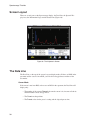
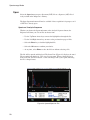
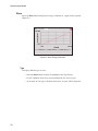
Screen Layout
There are several parts to the Spectroscopy display: the Data Line, the Spectral Display Area, the Information Pages and the Status Line (Figure 26).
Figure 26 The InSpector's Screen
The Data Line
The Data Line, at the top of the screen, has two display modes. If there are ROIs in the
spectrum and the cursor is in an ROI, you’ll be able to toggle between either of the
two modes.
Cursor Mode
If the cursor is not in an ROI, or there are no ROIs in the spectrum, the Data Line will
display only:
• The number of the current Channel, the one the cursor is in, in terms of both its
channel number and its energy in keV.
• The Counts at that position.
• The Preset values for the preset’s setting and the elapsed preset time.
30
The Data Line
ROI Mode (Shown in Figure 26)
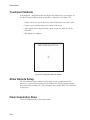
If the cursor is in an ROI, select the Down Arrow key to see:
• The Integral and Area of the current ROI, the one the cursor is in.
• The Preset values for the preset’s setting and the actual elapsed preset.
Selecting the Down Arrow key again will change back to the Cursor Mode.
Indexing the ROIs
When the Data Line is in the ROI Mode, you can Index (jump) from one ROI to another:
• Select the Right Arrow key to move to the next ROI to the right.
• Select the Left Arrow key to move to the next ROI to the left.
The Spectral Display
This area, in the middle of the display, shows the spectral data. Optional display
configurations are covered in Settings (page 81).
Frequently, there are ROIs (regions of interest) in a spectrum, as seen in Figure 26.
ROIs that have been associated with a nuclide are blue; ROIs that contain an unidentified peak are red.
The Information Pages
User selectable data about the current spectrum can be displayed below the spectrum
in an information page (page 77).
The Status Line
The Status Line at the bottom of the screen (Figure 27) displays several status indicators:
Figure 27 The Status Bar
• The current instrument status: Idle, Acquiring, High Field, Stabilized, Hold,
No Probe or ERROR.
31
Spectroscopy Tutorials
• The current analysis status: Analyzing or ERROR.
• The audio icons disable/enable an active Annunciator or Alarm/Warning audio
output.
u
The Annunciator output is active only if the Annunciator (page 19) has
been enabled. Selecting the audio icons
will turn the
Annunciator audio off and put a red X through the Annunciator icon.
u
If any enabled Warning or Alarm threshold is exceeded (page 91), its
programmed sound (page 99) will be heard.
Turning Off the Audio Alerts
u Selecting the audio icons a second time will turn the Alarms audio off
and put a red X through the Alarms icon.
u
Select the icons again to re-enable the first audio output, and a second
time to re-enable the second audio output.
u
If the Annunciator has not been enabled, its icon will always be disabled.
Only the Alarms icon can be toggled between on and off.
• There are two power icons: One
shows that the InSpector is using an
external power source; the other shows that the internal battery
is
powering the unit, and shows the battery charge remaining.
• A Help icon.
Select this button to display the help screen for the current
Mode or dialog screen.
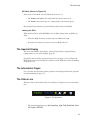
Error Messages
If a red NO PROBE appears in the status line, you must connect a probe to the InSpector before you can acquire data in the NID or Spec Modes.
If a red ERROR appears in the status line, there is an acquisition or analysis fault. Select the word “error” to open a text window describing the error (Figure 28)
32
Navigation
.
Figure 28 An Example of an Error Message
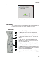
Navigation
There are two ways to navigate around the InSpector 1000’s menus and functions: by
the hard keys to the left of the display or by the soft buttons on the display.
Hard Keys
1. Power – Turns the InSpector On/Off.
2. Charge – Light whenever the battery is being charged.
3. Enter: – In a menu, executes the current soft key’s function;
when not in a menu, Starts or Stops data acquisition.
4. Up – Enters the main menu; in the menu, goes to the next
submenu.
5. Left – In the menu, moves left through the menu; in the
Cursor Mode (page 30), moves the plot cursor left; in the ROI
Mode, jumps one ROI to the left.
6. Right – In the menu, moves right through the menu; in the
Cursor Mode, moves the plot cursor right; in the ROI Mode,
jumps one ROI to the right.
7. Down – In the menu, goes to the previous menu level; if no
previous level, exits the menu. In the spectrum, toggles the data
line between Cursor Mode and ROI Mode.
8. Home – In the menu, exits the menu; otherwise, changes the
display to the “Home Mode” selected in Instrument Setup (page
98).
33
Spectroscopy Tutorials
Soft Buttons
The touchscreen allows both coarse control and fine control.
• Touch a soft button on the screen to select that button’s function.
• Touch the screen to position the cursor approximately in the spectrum.
• For fine control, use a stylus or your fingernail.
Moving the Spectrum’s Cursor
Touching the screen will move the Spec Mode’s spectrum cursor to an approximate
location. Then it can be moved more precisely with the front panel Left Arrow and
Right Arrow keys.
Accessing the Menus
You can move through the menus by:
• Selecting the screen soft buttons,
• Using the arrow hardkeys.
For example, selecting the Up Arrow shows you the first level menu with its four soft
buttons (Figure 29).
Figure 29 The First Level Menu
• The upward-pointing
triangle on the SPEC soft button indicates that there is
an another menu level associated with the button.
34
Navigation
• Select the SPEC button to see its next menu level. Figure 31 shows that each of
the first three menu buttons has another menu level.
Figure 31 The Spectroscopy Menu
• The last button has a right-pointing
more set of buttons at this level.
arrow, showing that there is at least one
• The area just below the menu displays the path you’ve followed to get to this
point. In this example, you can see that you have gotten here by having selected
SPEC.
• If you want to set the MCA’s preset parameters, select the MCA button in the
first spectroscopy menu level (Figure 30.)
Figure 30 The MCA Menu
35
Spectroscopy Tutorials
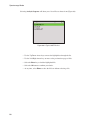
• In the next menu level, select Preset Time (Figure 33).
Figure 33 Preset Time Menu
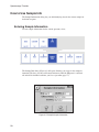
• This will open the MCA Presets dialog (Figure 35).
How to Acquire Data
To start acquiring data, select the Enter key.
Note: If the File | Open menu selection has been used to open a Spectrum (CNF) file,
data acquisition will be disabled.
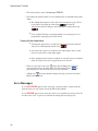
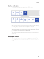
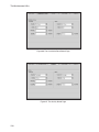
Starting Acquisition
When you select the Enter
key with acquisition off,
you’ll see Figure 32.
• You can start a New
acquisition.
• Or Save existing data
and start a new
acquisition.
36
Figure 32 Starting Data Aquisition
How to Navigate a Parameters Dialog
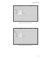
Stopping Acquisition
When you select the Enter
key with acquisition on,
you’ll see Figure 34.
• You can stop
acquisition and Clear
data.
• You can Stop
acquisition without
clearing data.
Figure 34 Stopping Data Acquisition
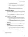
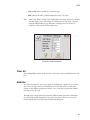
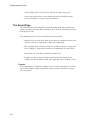
How to Navigate a Parameters Dialog
To navigate a Parameters Dialog, such as MCA Presets (Figure 35):
• Select the Enter key to
move the highlight to
the first text box,
Time.
• Each time you select
the key, the highlight
will move down one
text box at a time, then
to the soft buttons,
then back to the top of
the dialog.
• To cancel a dialog box
without savings any
changes, select the
Home key, the Cancel
button, or the
red
in the upper
right corner of the dialog.
Figure 35 A Typical Parameters Dialog
Changing a Numeric Parameter
• Move the highlight to a numeric text box (for instance, Time). Only the first
digit is highlighted, showing that this is a numeric parameter.
• Use the Up/Down Arrow keys to increase/decrease the value of the highlighted
digit.
37
Spectroscopy Tutorials
• Use the Left/Right Arrow keys to move forward/back through the digits.
• Repeatedly select the Enter key until the Ok and Cancel buttons are
highlighted, then select the Up Arrow (Ok) to apply the change.
Note: If you enter an invalid value, the system will change it to the closest valid
value when you select Enter.
The Virtual Keyboard
Numeric parameters can also be changed by selecting the virtual keyboard icon
the upper right corner of the screen. Using a stylus (or a fingernail):
in
• Select the left or right arrow key in the lower right corner of the keyboard to
position the highlight.
• Select a digit, 0–9, to change the digit’s value.
• Select an arrow key to move to the next position to be changed.
• To correct an error, use the backspace key to delete the character to the left of
the cursor.
• When done, select the keyboard icon to close the keyboard.
Changing a List Parameter
• Move the highlight to a serial selection text box, such as Mode. The entire
parameter is highlighted, showing that this is a list parameter.
• Select the Up or Down Arrow key to move through the parameter list. For
Mode, for instance, the selections are Real, Live and Continuous.
• When the parameter has been selected, repeatedly select the Enter key until the
Ok and Cancel buttons are highlighted, then select the Up Arrow (Ok) to apply
the change.
38
How to Verify Spectroscopy Parameters
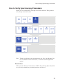
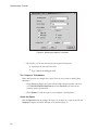
How to Verify Spectroscopy Parameters
Before you start acquiring data, you might want to check the Preset Time parameter.
Select the Up Arrow, then select:
Note: To show you all items at the same menu level, the “Next” and “Previous” buttons are omitted from these illustrations, a convention used throughout this
manual.
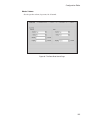
Preset Values
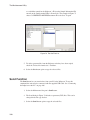
When you select the Preset Values button, the MCA Presets dialog (Figure 36), which
lets you verify or modify the preset time parameters, will be seen.
39
Spectroscopy Tutorials
• Time – The amount of
time in the selected
Units to pass before
acquisition ends.
• Units – The preset’s
time units.
• Mode – Live time,
Real time or
Continuous
acquisition.
Figure 36 Preset Values
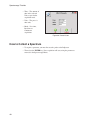
How to Collect a Spectrum
• To acquire a spectrum, you must first attach a probe to the InSpector.
• Then select the ENTER key. Data acquisition will start, using the parameters
entered via the Spectroscopy Menu.
40
How to Load a Calibration File
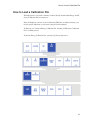
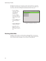
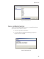
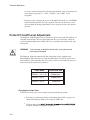
How to Load a Calibration File
The InSpector lets you Load a memory-resident (already downloaded) Energy or Efficiency Calibration file for current use.
Since the InSpector can have several calibration (CAL) files resident in memory, you
need to specify which one is to be used, using the Load command.
To illustrate, we’ll load an Energy Calibration file. Loading an Efficiency Calibration
file is a similar process.
To load an Energy Calibration file, select the Up Arrow, then select:
41
Spectroscopy Tutorials
The InSpector will show you a list of files to choose from. To illustrate a typical file
list, Figure 37 shows the energy calibration files for each probe type. You don’t need
to select one of these files; the InSpector automatically uses the correct one.
• Use the Up/Down
Arrow keys to move
the highlight bar
through the list.
• Use the Left/Right
Arrow keys to move to
the previous/next page
of files.
• Select the Enter key to
load the highlighted
file.
• Select the Ok button to
confirm your choice.
Figure 37 Illustration of a File List
• At any time, select
Home to close the file
box without selecting a
file.
Working With ROIs
An ROI is a region of interest, usually marking a photopeak. There are two ways to
enter ROIs in your spectrum: you can run an analysis (ASF) routine containing Peak
Locate and Peak Analysis algorithms or you can load an existing ROI file.
42
Working With ROIs
Creating ROIs With an Analysis Routine
To create ROIs in the current spectrum via an analysis sequence (ASF) file. To open
an analysis sequence file, select the Up Arrow, then select:
43
Spectroscopy Tutorials
The InSpector will show you a list of files to choose from (Figure 38).
• Use the Up/Down
Arrow keys to move
the highlight bar
through the list.
• Use the Left/Right
Arrow keys to move to
the previous/next page
of files.
• Select the Enter key to
load the highlighted
file.
• Select the Ok button to
confirm your choice.
Figure 38 An ASF File List
• At any time, select
Home to close the file
box without selecting a
file.
Starting the Analysis Sequence
Now select the Up Arrow again and select:
The analysis sequence file you loaded will be executed and all found peaks will have
ROIs entered around them.
44
Working With ROIs
Note: The analysis may take some time to complete, depending on the number and
complexity of its steps.
Color of the ROIs
The analysis routine will mark each found peak with an ROI (region of interest). Peaks
associated with an identified nuclide will be marked with a blue ROI. Peaks that cannot be identified will be marked with a red ROI.
Loading ROIs From an ROI File
ROIs can be added to a spectrum by loading an ROI (region of interest) file. To load
the ROIs, select the Up Arrow, then select:
45
Spectroscopy Tutorials
The InSpector will show you a list of files to choose from (Figure 39).
• Use the Up/Down
Arrow keys to move
the highlight through
the list.
• Use the Left/Right
Arrow keys to move to
the previous/next page
of files.
• Select the Enter key to
load the highlighted
file.
• Select the Ok button to
confirm your choice.
Figure 39 An ROI File List
• At any time, select
Home to close the file box without selecting a file.
Note: If ROIs loaded from a file are present in a spectrum, they will prevent the display of ROIs generated from an analysis routine. Clearing the loaded ROIs will
allow the generated ROIs to be displayed.
Deleting One ROI
Select Delete to remove the current ROI, the one with the cursor in it, from the display. The ROI’s data will not be changed.
Clearing All ROIs
Select Clear to remove all ROIs from the spectrum. The ROIs’ data will not be
changed.
46
How to Analyze a Spectrum
How to Analyze a Spectrum
Spectrum analysis is performed by an analysis sequence file (ASF). The InSpector always has at least one ASF loaded
How to Select a Different Sequence File
Since the InSpector can include several ASF files, there may be a time when you need
to change the one being used.
To load another ASF, select the Up Arrow, then select:
47
Spectroscopy Tutorials
The InSpector will show you a list of files to choose from (Figure 40).
• Use the Up/Down
Arrow keys to move
the highlight bar
through the list.
• Use the Left/Right
Arrow keys to move to
the previous/next page
of files.
• Select the Enter key to
load the highlighted
file.
• Select the Ok button to
confirm your choice.
Figure 40 A Typical ASF File List
• At any time, select
Home to close the file
box without selecting a
file.
How to Start the Analysis
With a spectrum present on the screen, select the Up Arrow, then select:
The spectrum will be analyzed according to the instructions in the currently selected
ASF.
48
How to Analyze a Spectrum
During an acquisition and analysis, you can switch to NID mode in order to view the
existing NID results which are updated as soon as the latest analysis sequence has finished execution.
How to Stop the Analysis
When the Analyze button is selected, its legend changes from start to abort. So to stop
an executing analysis, all you have to do is select the Analyze button again. The analysis will stop.
49
Spectroscopy Tutorials
How to Use Sample Info
The Sample Information dialog lets you add identifying data for the current sample for
inclusion in reports.
Entering Sample Information
To enter sample information for the current spectrum, select:
The Sample Info dialog (Figure 41) will open, allowing you to type in the sample information. The data you enter will remain in memory until the InSpector is switched
off and will be included each time you Save a spectrum (page 57).
Figure 41 Example Sample Information
50
How to Use Sample Info
• ID is a sample identification of your choice.
• Quantity lets you enter the sample’s quantity. Calculated activities are divided
by this value, so that if the quantity is set to 1 (the default), total activity is
reported. If any other value is entered, concentration is reported.
• Collector Name lets you enter the name of the person who collected the
sample.
• Location is a description of the place where the sample was collected.
Transferring the Spectrum
Use the Maintenance Utility’s Get function (page 107) to copy the current spectrum to
the In1kname folder on your PC*, where name is the Instrument ID assigned on the
General page of the Configuration Editor (page 117) or during a software update.
The file’s name will be filename.cnf, where filename is the date and time of the file’s
creation: YYYYMMDDHHMMSS.cnf (Year, Month, Day, Hour, Minute, Second).
Creating the Report in Genie 2000
To create the Example Report shown on page 53 from the transferred spectrum file:
• In Genie 2000, select File | Open, then select filename.cnf to open the file you
transferred.
• Select Analyze | Report | Standard (Figure 42) to open the Standard Report
Setup dialog and select the parameters for generating the report.
Template Name
Scroll down the Template Name list to find and select the 1page.tpl report template.
Section Name
Scroll down the Section Name list to find and select the 1page report section.
The Activity Units
• Activity is reported in microcuries by default. (The Activity Units field is uCi
and the Multiplier is 1).
• If you want to use another Activity Unit, you’ll have to supply a Multiplier to
convert the activity from microcuries to your unit.
*The standard path for this folder is in C:\Genie2k\Camfiles. If you didn’t select the Standard installation for
Genie 2000, your path will be different.
51
Spectroscopy Tutorials
Figure 42 Selecting the Report's Parameters
• For instance, if you want the activity to be reported in bequerels:
u
Type Bq in the Activity Units field.
u
Type 37000 in the Multiplier field.
The “Output to” Checkboxes
Genie 2000 provides two outputs for a report. You can select either or both of their
checkboxes.
• Check Screen to display the report in Genie 2000’s Report window and file it
as C:\Genie2k\Repfiles\filename.rpt, where filename is the name of the
currently opened spectrum file.
• Check Printer to send the report to your computer’s default printer.
Create the Report
Click the Execute button to generate the report. An example of a report created by the
1page.tpl Template you chose in Figure 42 is shown on page 53.
52
How to Use Sample Info
Example Report
Interference Corrected Activity Report
3/09/2004
11:46:04
Page
1
*************************************************************************
*****
N U C L I D E
I D E N T I F I C A T I O N
R E P O R T
*****
*************************************************************************
Filename: C:\GENIE2K\CAMFILES\02047924\20040903114041.cnf
Sample Title
Sample Identification
Sample Size
Operator Name
Location
:
:
:
:
:
InSpector 1000 spectrum
Enter ID
1.2300E+02
Collector’s name
Collected at
Acquisition Started, detector
Live Time, Dead time
: 3/09/2004 10:53:50
:
192.5 seconds,
Analysis Sequence Title
Identification Energy Tolerance
Env. Background File
Nuclide ID Library Used
Efficiency ID
: NaI Analysis
:
0.250 FWHM
:
<not performed>
: \GENIECE\CAMFILES\NaI_ANSI_4.NLB
: POINT_@1M_1G/CC
,
Scionix2x2
0.41 %
*************************************************************************
*****
I N T E R F E R E N C E
C O R R E C T E D
R E P O R T
*****
*************************************************************************
Nuclide
Name
K-40
Cs-137
Nuclide
Id
Confidence
0.982
0.990
Wt mean
Activity
(Bq /S. Size)
2.206E+04
2.442E+05
Wt mean
Activity
Uncertainty
Wt mean
Activity
Uncertainty%
2.933E+03
7.025E+03
13.30
2.88
? = nuclide is part of an undetermined solution
X = nuclide rejected by the interference analysis
@ = nuclide contains energy lines not used in Weighted Mean Activity
Uncertainty quoted at
**********
Peak
No.
F
F
1
2
1.000 sigma
U N I D E N T I F I E D
Energy
(keV)
73.97
435.76
P E A K S
Peak Size in
Counts per Second
3.692E+00
1.128E+01
**********
Peak CPS
% Uncertainty
16.28
5.36
M = First peak in a multiplet region
m = Other peak in a multiplet region
F = Fitted singlet
53
Spectroscopy Tutorials
CAM Parameters
For reporting purposes, these CAM variables are used:
54
Inspector Data Field
CAM Parameter
ID:
CAM_T_SIDENT
Quantity:
CAM_F_SQUANT
Collector Name:
CAM_T_SCOLLNAME
Location:
CAM_T_SLOCTN
8. Spectroscopy Mode
The Spectroscopy Mode lets you acquire and display data and analyze either the current spectrum or a spectrum file.
The Spectroscopy Mode functions of the InSpector™ parallel the same functions in
the Genie 2000 Spectroscopy Software. For detailed information, please refer to the
Genie 2000 Operations Manual and the Genie 2000 Customization Tools Manual.
Both are included as PDF files on your Genie 2000 CD-ROM.
Memory Resident Files
Several of the InSpector’s functions require choosing a file resident in the InSpector’s
memory as the current file, the one to be used for that function. The Maintenance Utility’s Send command (page 105) transfers files from your PC to the InSpector’s memory.
Hard Key Functions
1. Power: Turns the InSpector On/Off.
2. Charge: Light whenever the battery is being charged.
3. Enter: Starts or Stops an acquisition.
4. Up: Enters the main menu; in the menu, goes to the next
submenu.
5. Left: In the menu, moves left through the menu; in the Cursor
Mode (page 30), moves the plot cursor left; in the ROI Mode,
jumps one ROI to the left.
6. Right: In the menu, moves right through the menu; in the Cursor Mode, moves the plot cursor right; in the ROI Mode, jumps
one ROI to the right.
7. Down: In the menu, goes to the previous menu level; if no previous level, exits the menu. In the spectrum, toggles the data line
between Cursor Mode and the ROI Mode.
8. Home: In the menu, exits the menu; otherwise, changes the
display to the “Home Mode” selected in Instrument Setup (page
98).
55
Spectroscopy Mode
Alarms
If the warning and/or alarm thresholds for Dose Rate, Cumulative Dose and/or Neutron Count Rate (page 91) are exceeded, you will be alerted to the condition in several
ways.
Warning Indicator
If the low-level Warning threshold is exceeded,the spectral display’s background will
alternate between black and gold.
Alarm Indicator
If the high-level Alarm threshold is exceeded, the spectral display’s background will
alternate between black and maroon.
The Spectroscopy Mode Menus
Each of the remaining sections in this chapter describes the Spectroscopy Mode’s
menus and the use of their selections.
• File
• MCA
• Calibrate
• Sample Info
• Info (display pages)
• Display
• Analyze
56
File
File
The File menu is used to Open or Close a file, Save the current file, or Delete it from
memory.
Save
Select Save to save the current spectrum to Genie 2000’s C:\Genie2K\Camfiles directory.
Note: This is the directory created by a Standard Genie 2000 installation. If you
chose Custom installation, your path for storing spectrum files may be different.
Spectrum File Name
The file name is created from the file’s date/time stamp: YYYYMMDDHHMMSS.cnf
(Year, Month, Day, Hour, Minute, Second).
The file will contain the spectrum’s raw data, the results, all the current context parameters, based on the current Analysis file, any parameters changed in Setup | Spec Setup
(page 96), and the data entered in Sample Info (page 76).
57
Spectroscopy Mode
Open
Select the Open button to open a Spectrum (CNF) file or a Sequence (ASF) file already resident in the InSpector’s memory.
The Open Spectrum button will not be available if data acquisition is in progress or if
a CNF file is already open.
Spectrum / Analysis Sequence
Whether you choose the Spectrum button or the Analysis Sequence button, the
InSpector will show you a list of files to choose from.
• Use the Up/Down Arrow keys to move the highlight bar through the list.
• Use the Left/Right Arrow keys to move to the previous/next page of files.
• Select the Enter key to load the highlighted file.
• Select the Ok button to confirm your choice.
• At any time, select Home to close the file box without selecting a file.
The file will be opened and displayed. The Status Line (Figure 43) displays the word
File to remind you that this is a file, not a live spectrum. When a change has been
made to the file, the File indicator’s color will change from cyan to gold, indicating
the file’s changed status.
Figure 43 Opened Spectrum File
58
MCA
Close
Select Close to close the spectrum most recently opened from a file. This command is
available only if a file has been opened.
Note: An acquired spectrum cannot be closed; you can only Save it.
Delete
When you choose to Delete a file, the InSpector will show you a list of spectrum files
to choose from.
• Use the Up/Down Arrow keys to move the highlight bar through the list.
• Use the Left/Right Arrow keys to move to the previous/next page of files.
• Select the Enter key to delete the highlighted file.
• Select the Ok button to confirm your choice.
• At any time, select Home to close the file box without deleting a file.
MCA
The MCA Menu lets you select the Preset Time, change some of the InSpector’s settings, clear the display, and use the instrument’s Stabilizer.
59
Spectroscopy Mode
Preset Time
The Preset Time command lets you define the period of time allowed for data collection.
Preset Values
The Preset Values command defines the absolute time, the time units and the preset
mode.
If you enter the preset using units other than seconds, the time will be converted to and
stored as the equivalent number of seconds when you select Ok.
• Time – Selects the value of preset time. The combination of Time and Units
determines how long data acquisition will continue.
• Units – Selects the preset’s units of time.
• Mode – Selects the mode of operation:
u
Real – Counts to the specified elapsed real time.
u
Live – Counts to the specified elapsed live time.
u
Continuous – Counts until the Enter key is pressed to stop acquisition.
When this Mode is selected, the values for Time and Units are ignored.
Preset Mode
This button gives quick access to the Mode command in MCA Presets. It toggles the
preset type between real, live and continuous (defined in the previous paragraphs).
Hardware Settings
The initial Hardware Settings shown in Figure 44 are based on the current probe and
on the energy range and memory size (number of channels) set in the MCA Page of
the InSpector’s Configuration Editor (page 121).
Though you can change the parameters here, it’s generally best to leave the high voltage at its default setting for the attached probe and to leave the Coarse and Fine Gain
set at 1.
• High Voltage: Sets the detector’s high voltage. (Not available if a Stabilized
Probe is attached to the InSpector.)
• Coarse Gain: Sets the amplifier’s coarse gain.
• Fine Gain: Sets the amplifier’s fine gain.
• ADC Gain: Sets the ADC’s gain.
60
MCA
• Conv. Gain: Selects the MCA’s conversion gain.
• LLD: Adjusts the ADC’s LLD threshold; the range is 0–100%.
Note: If the Conv. Gain is adjusted, the relationship between the spectrum’s channels
and their energy levels will change. To compensate for this effect, you must
perform a Manual Recal (page 68) before acquiring new data. Failure to
recalibrate will result in invalid sample data.
Figure 44 Hardware Settings
Clear All
Select Clear All to remove all spectral data and analysis-generated ROIs from the display.
Stabilize
In certain circumstances, the energy output of the InSpector’s probe can vary (drift),
such as in very high count rate environments or if the probe warms or cools with
changes in the ambient temperature. In these cases, some type of spectrum stabilization may need to be used.
The InSpector’s integrated digital spectrum stabilizer allows for probe stabilization
over the full operating temperature range of the instrument. This is an easy-to-use
method which allows selection of the stabilization photopeak.
61
Spectroscopy Mode
The InSpector achieves stabilization by continuously monitoring an energy “window”
set around the selected stabilization peak and adjusting the probe’s high voltage to
maintain the peak in the proper position. The optimal width of the energy window is
determined automatically by the software.
Using a Stabilized Probe
The Stabilized Probe is very easy to use. When the InSpector finds a Stabilized Probe
connected to its DET connector, it will display a message for about 30 seconds, advising you that the probe is stabilizing (Figure 45).
Figure 45 The Probe is Stabilizing
• The blue LED on the probe will blink while stabilization is in process. When
stabilization is complete, the LED will glow steadily.
• If stabilization is lost, perhaps due to moving the unit from a warm environment
to a cold one (indoors to outdoors), data acquisition will stop and the instrument
will restabilize itself (the blue LED will start blinking). When the LED glows
steadily, stabilization is complete and acquisition can be restarted.
• If you enter a high radiation area, High Field will be displayed at the bottom of
the screen, data acquisition will stop, the probe’s high voltage and its blue LED
will be turned off. When you leave the High Field area, the high voltage will be
turned on again and the LED will start blinking as the probe begins stabilizing.
When the LED glows steadily, stabilization is complete and acquisition can be
restarted.
62
MCA
Using the Stabilize Function
Note: The Stabilize function is available only when one of the standard Gamma
Probes is being used. The function is disabled when a Stabilized Probe is attached to the InSpector.
In order to turn on stabilization, you must acquire a spectrum and choose the peak
whose position is to be held constant
1. To start the process, select:
63
Spectroscopy Mode
2. The InSpector will ask you to Select the stabilization reference peak in the
spectrum (Figure 46), then press the ENTER key.
Figure 46 Select the Reference Peak
Note: The selected stabilization peak must always be present and free from interference from nearby peaks while stabilization is on.
3. An ROI will be painted on the peak’s stabilization window. The InSpector
will ask you to Accept the reference peak by selecting the Up Arrow (Figure
47). Stabilization will start.
Figure 47 Accepting the Stabilizer Peak
The Stabilizer is now On. If you re-enter the Stabilize menu, you’ll see that you can
choose only Hold or Off.
Stabilization On will automatically be switched to Off:
• If the High Voltage or any of the Gains are manually adjusted.
• If one of the Recal functions is executed.
• If you enter a high dose rate field.
• If you disconnect / connect the probe.
Stabilization Hold will automatically be switched to Off if the high voltage, gain or
LLD settings are manually adjusted.
64
Calibrate
Calibrate
The Calibrate menu offers both Energy and Efficiency calibration.
Energy Calibration establishes a relationship between the spectrum’s channels and
their energy levels. By calibrating at least three peaks over the entire range of the spectrum, the energy of any other peak can be reliably estimated.
Efficiency Calibration establishes a relationship between measured count rate and
source activity as a function of energy. The efficiency calibration allows us to convert
count rates to activities for various source nuclide energies.
Energy
The Energy Menu command lets you load a memory-resident calibration (CAL) file,
recalibrate the InSpector, show a calibration graphically, display and edit the Energy
or Shape (FWHM) calibration’s coefficients, and perform a full calibration.
65
Spectroscopy Mode
Load
To illustrate a typical file list, Figure shows the energy calibration files for each probe
type. You don’t need to select one of these files; the InSpector automatically uses the
correct one.
• Use the Up/Down Arrow keys to move the highlight bar through the list.
• Use the Left/Right Arrow keys to move to the previous/next page of files.
• Select the Enter key to load the highlighted file.
• Select the Ok button to confirm your choice.
• At any time, select Home to close the file box without selecting a file.
Recalibrating the InSpector
Sodium iodide (NaI) detectors, the kind used by the InSpector, can experience “peak
drift” with a change in temperature or due to aging. This is easily compensated for by
placing a calibration source in front of the detector and selecting one of the
recalibration buttons to correct for the drift.
Auto Recal
Auto Recal automatically adjusts the probe’s gain or high voltage so that the energy
calibration is valid, correcting for shifts due to temperature or tube aging. To provide
Auto Recal with the best possible data, Auto Recal should always be done in a low
background area.
If there are many other peaks in the window due to environmental background, or if
the calibration peak has drifted too far from its predicted position, the Auto method
may not be able to find the peak. In either case, you should use Manual Recal instead.
1. When you start Auto Recal, you’ll be prompted to place a mono-line
calibration source (10 to 20 nCi) in front of the detector (Figure 48).
66
Calibrate
Figure 48 The Calibration Prompt
The most useful calibration source is a cap with a built-in source that fits
over the end of the probe, such as the Model CSRCSS-n, where the ‘n’
matches the Probe’s model number. For example, the Model CSRCSS-1 is
used with the IPRON-1 probe.
2. The InSpector will make a brief measurement, then analyze the spectrum for
peaks and attempt to locate the calibration peak. If the peak cannot be found, a
longer measurement will be made. If the peak still cannot be found, the
InSpector will report the problem; see Peak Not Found, below, for what to do.
3. You can abort this measurement at any time by selecting the Home button.
4. The detector gain and/or voltage are adjusted so that the peak will appear in
the correct spot in the spectrum. If the voltage had to be adjusted, steps 2 and
3 will be repeated to fine tune the adjustment.
5. If there are multiple peaks in the spectrum, the InSpector may not be able to
pick out the calibration peak. The InSpector will indicate that this has
occurred. Check the calibration to see if other peaks appear at the correct
energies. If not, use Manual Recal to manually select the calibration peak.
Peak Not Found
If the InSpector cannot find the calibration peak, you should:
1. Make sure that the calibration source is present.
67
Spectroscopy Mode
2. Examine the spectrum. If the continuum is very high, the calibration peak
may be obscured; move to a location with a lower background rate and
repeat Auto Recal.
3. Try to find the calibration peak in the spectrum; it may have shifted outside
Auto Recal’s range. In this case, use Manual Recal, to manually identify the
peak.
The energy of the calibration peak, the amount of shift that Auto Recal can handle,
and the strength of the calibration peak can be set in Calibration Setup on page 97.
Manual Recal
The Manual Recalibration function is used to adjust the gamma probe’s high voltage
bias so that the energy calibration is valid, correcting for shifts due to temperature or
tube aging. To use Manual Recal, you must be able to locate the calibration peak in the
spectrum yourself.
Spectrum Present
If you have a spectrum, you’ll be asked to position the cursor on the 662 keV peak
(Figure 49), then select Enter. Follow the instructions on the screen.
Figure 49 Manual Recalibation
68
Calibrate
Spectrum Not Present
If there is no spectrum, you’ll be prompted to acquire one by placing a mono-line calibration source (10 to 20 nCi) in front of the detector (Figure 50).
Figure 50 The Calibration Prompt
The most useful calibration source is a cap with a built-in source that fits over the end
of the probe, such as the Model CSRCSS-n, where the ‘n’ matches the Probe’s model
number. For example, the Model CSRCSS-1 is used with the IPRON-1 probe.
1. Select OK to start Data Acquisition.
2. You can press the Home key at any point in this process to abort the
operation.
3. Find the calibration peak in the spectrum and position the cursor on it using
the Left or Right Arrow keys or by touching the screen.
4. Press the Enter key. The InSpector will adjust the probe so that the peak will
appear in the right place in the spectrum and the energy calibration is valid.
5. If peak has shifted a large amount, the InSpector may have to adjust the
probe’s voltage; this is not as accurate as adjusting the probe gain. The
InSpector will inform you that the voltage was changed, and you should
repeat Manual Recal to fine tune the adjustment.
69
Spectroscopy Mode
Show
Select the Show button to display the energy calibration as a graph and its equation
(Figure 51).
Figure 51 Show Energy Calibration
Type
To display different type of curve:
• Select the Enter button to move the highlight to the Type list box.
• Use the Up/Down Arrow keys to move through the list of curve types.
• As the name of each type is shown in the list box, its curve will be displayed.
70
Calibrate
Coeff
The Coefficients screen (Figure 52) lets you view or manually enter the Offset, Slope
and Quadratic coefficients for the Energy Calibration and the Offset and Slope coefficients for the FWHM calibration.
Figure 52 Energy Coefficients
Full
Select Full energy calibration to fine-tune the detector’s energy calibration. It can also
be used on a stored spectrum file. The calibration process requires a multi-photopeak
calibration source, such as Canberra’s Model MGS-3 Calibration Standard, and assumes that the existing calibration parameters are not too far off; that is, that the calibration source peaks can be found relatively close to their predicted positions.
The function uses a wizard (Figure 53) to step through the calibration process. The
Right and Left Arrow keys will step to the next or previous step of the process. Select
the Home key at any time to abort the calibration.
71
Spectroscopy Mode
Figure 53 Full Calibration Setup Wizard
1. First indicate the source of the calibration energies: either a Certificate File,
or a Nuclide Library.
u
If Certificate File was selected, choose the file that contains the
calibration source’s photopeak energies.
u
If Nuclide Library was selected, select the library which contains the
nuclides in the calibration source. The wizard's next step will list the
nuclides in the library. To choose a nuclide, use the Up and Down
Arrow keys to highlight the nuclide, then select Enter. Selected
nuclides will be highlighted in yellow.
2. When all nuclides have been selected, their photopeak energies are extracted
from the library and sorted. Any overlapping energies (those within 1.5
FWHM of each other) will be discarded. At least three energies are required.
Note that a certificate file will automatically be created; the file contains the
photopeak energies of the selected nuclides. The name of the file is created
using the names of the selected nuclides.
3. Select the “peak match tolerance”; this determines how far from its predicted
position each calibration peak can be and still be considered a valid peak. To
change the tolerance value, select the Enter key to highlight the FWHM
value, then edit the value. Select Enter to move the highlight to the Previous
and Ok buttons, and then select the Right Arrow key to proceed.
A larger tolerance value allows more variation between the current
calibration and the actual position of the peaks, but also increases the
possibility of false matches.
72
Calibrate
If “Do FWHM Calibration?” is set to Yes, a FWHM calibration will be
performed at the same time. Set this parameter to No to perform only the
energy calibration.
4. To calibrate the probe, place the calibration source on the detector when
prompted, then select Ok to start acquisition. When you judge that sufficient
data has been collected, press Enter to stop the acquisition.
5. The peaks found in the spectrum will be matched against the photopeak
energies specified in the certificate or nuclide library, new calibration
coefficients calculated, and the resulting plot of channel vs. energy
displayed. If the results are acceptable, press the Up Arrow to save the
calibration and the calibration spectrum file; otherwise, press the Down
Arrow to discard it.
If fewer than three calibration peaks are sufficiently close to their predicted
positions, the calibration wizard will report an error. You can try again, using
a larger tolerance (see step 3) or use one of the RECAL functions to shift the
entire spectrum closer to the current calibration.
73
Spectroscopy Mode
Efficiency
The Efficiency Menu command lets you load a memory-resident (already downloaded) CAL file or show a calibration graphically.
Load
When you select Load, the InSpector will show you a list of files to choose from.
• Use the Up/Down Arrow keys to move the highlight bar through the list.
• Use the Left/Right Arrow keys to move to the previous/next page of files.
• Select the Enter key to load the highlighted file.
• Select the Ok button to confirm your choice.
• At any time, select Home to close the file box without selecting a file.
74
Calibrate
Show
Select Show to display the efficiency calibration as a graph and its equation (Figure
54).
Figure 54 Show Efficiency Calibration
Model
This screen allows you to choose a different Model for the displayed curve: Dual,
Linear, Empirical or Interpolated.
To choose a different model, press the Enter button. The model you choose is valid
only for the current Show display; the model will default to Dual the next time you
open the Show screen.
Note: The chosen model affects only the current Show display; the model used for
analysis is set in the analysis sequence’s efficiency step.
For technical information about the four efficiency models, refer to Efficiency Calibration Models on page 145.
75
Spectroscopy Mode
Sample Info
The Sample Info dialog lets you enter information about the current spectrum.
The Sample Info dialog (Figure 55) lets you to enter information about the current
sample. The data you enter will remain in memory until the InSpector is switched off
and will be included each time you Save a spectrum (page 57).
Figure 55 Sample Information
76
Info
• ID is a textual sample identification of your choice.
• Quantity lets you enter the sample’s quantity. Calculated activities are divided
by this value, so that if the quantity is set to 1 (the default), total activity is
reported. If any other value is entered, concentration is reported.
• Collector Name lets you enter the name of the person who collected the
sample.
• Location is a description of the place where the sample was collected.
Info
Detailed information about the current datasource can be seen in the Info page you
choose to display.
Each press of the Info button toggles which Info page is displayed below the spectrum.
Each page is described in the following sections.
None
Select None to remove the Info pages from the display; this makes the spectral display
larger.
77
Spectroscopy Mode
ROI
The ROI page (Figure 56) shows the Left and Right limits and Centroid of the current
ROI, both as a channel number and an energy, the ROI’s Area, its Integral, and its
FWHM (full width at half max) and FWTM (full width at tenth max) values. This data
will be seen only if the cursor is in an ROI.
Figure 56 The ROI Page
Calibration
The Calibration page (Figure 57) includes the current calibration’s Energy equation,
FWHM (full width at half max) equation, and the Efficiency at the cursor’s position
and its curve model.
Figure 57 The Calibration Page
Time
The Time page (Figure 58) includes the Start time for the current data Acquisition, the
percent Dead Time, and the Elapsed and Preset values for both Live Time and Real
Time.
Figure 58 The Time Page
78
Info
Display
The Display page (Figure 59) includes the display window’s Start and End Channels
by number and energy, the display’s current VFS (vertical full scale) and, if the cursor
is in an ROI, its Net and Total CPS (counts per second).
Figure 59 The Display Page
Nuclide
The Nuclide page (Figure 60) includes the Analysis Sequence description, the Identified nuclide at the cursor’s position and any other potential nuclides found In Library.
Figure 60 The Nuclide Page
Sample
The Sample page (Figure 61) describes the current sample’s descriptive information
that will be saved with spectral data. This data is used in reports when saved spectra
are uploaded to a host PC. None of these values have any significance in analysis except the quantity.
Figure 61 The Sample Page
• ID, an identifier for the sample being measured, Quantity, the amount of sample
being measured, and Quantity Units if specified, are taken from data entered in
Sample Info (page 76).
• Type is taken from Sample Information data entered on the General page of the
InSpector’s Configuration Editor (page 117); it cannot be entered directly in the
InSpector.
79
Spectroscopy Mode
• Geometry displays the data entered in the Eff Geom ID field in Genie 2000’s
Calibrate | Store menu command.
• Time is the time the sample was taken.
• Efficiency is the name of the file used to efficiency calibrate the sample.
Display
The Display menu includes Zoom commands, display Settings and ROI commands.
Zoom
The Zoom command reformats the spectral display, centered on the cursor, to show
more or less detail.
80
Display
Zoom None
The Zoom None command disables the zoom ratio, returning the spectrum to its normal appearance.
Zoom In
Each time the Zoom In command is selected, the zoom ratio is increased, showing a
smaller amount of the spectrum in greater detail.
Zoom Out
Each time the Zoom Out command is selected, the zoom ratio is decreased, showing a
greater amount of the spectrum in less detail.
Settings
The Settings parameters configure the appearance of the display.
81
Display
Scale
Each time the Scale command is selected, the spectrum’s XY-scales toggle between:
linlin, linlog, loglin, loglog, sqrtlin and sqrtlog.
Borders
The Borders command toggles the display’s X- and Y-axis borders between visible
and none (Figures 62 and 63).
Figure 62 Visible Borders
Figure 63 No Borders
Plot Type
The Plot Type command toggles the way the spectrum is displayed between line, area
and points.
Line
Line displays the spectrum as a solid line (Figures 62 and 63).
82
Display
Area
Area displays the spectrum with the area filled in (Figure 64).
Figure 64 Display Spectrum as Area
Points
Points displays the data as points on a plot (Figure 65).
Figure 65 Display Spectrum as Points
83
Spectroscopy Mode
Gridlines
The Gridlines command toggles the display’s X-Y gridlines between enable and disable (Figure 66).
Figure 66 Gridlines Enabled
X-Units
The X-Units command toggles the X-axis’ label between channels (Figure 66) and energy (Figure 65).
Autoscale
The Autoscale command lets the program automatically set the display’s vertical full
scale (VFS) As the spectral data increases, the VFS is automatically reset to show all
of the data.
Max-Y
If Autoscale is not enabled, Max-Y lets you specify the absolute value of the Y-axis
scale.
84
Display
ROI
An ROI is a region of interest, usually marking a photopeak. You can create ROIs by
executing an analysis sequence file containing Peak Locate and Peak Analysis algorithms (page 43) or you can load the ROIs from a file (page 45).
Color of the ROIs
Peaks associated with an identified nuclide will be marked with a blue ROI. Peaks
that cannot be identified will be marked with a red ROI.
To access the ROI menu, select the Up Arrow, then select:
Delete
When the cursor is in an ROI, the Delete button will be enabled; selecting the button
will delete the current ROI from the display.
85
Spectroscopy Mode
When the cursor is not in an ROI, the Delete button will be disabled; the button cannot
be selected.
Clear
Selecting Clear will remove all ROIs from the spectrum, whether entered by an analysis routine or loaded from a file.
Load
Selecting Load will show you a list of ROI files to choose from (Figure 67):
Figure 67 A Typical ROI File List
• Use the Up/Down Arrow keys to move the highlight bar through the list.
• Select the Ok to load the highlighted file.
• Use the Left/Right Arrow keys to move to the previous/next page of files.
• Select the Enter key to load the highlighted file.
• Select the Ok button to confirm your choice.
• At any time, select Home to close the file box without selecting a file.
Note: If ROIs loaded from an ROI file are present in a spectrum, they will prevent
the display of ROIs generated from an analysis routine. Clearing the loaded
ROIs will allow the generated ROIs to be displayed.
86
Analyze
Analyze
The InSpector can perform a full gamma spectroscopy analysis, including peak location and analysis, environmental background subtraction, efficiency calculation, and
nuclide identification and activity calculation. This analysis is performed via Analysis
Sequence (ASF) files using Genie 2000 algorithms Genie. Each file defines a series of
analysis steps and the parameters used by each.
For a discussion of using Genie 2000 to create or edit an ASF, refer to Appendix E,
Using ASFs, on page 162.
Loading the Sequence File
Analysis requires that a memory-resident sequence file (ASF) be loaded. Select the Up
Arrow, then select:
87
Spectroscopy Mode
Selecting Analysis Sequence will show you a list of files to choose from (Figure 68).
Figure 68 A Typical ASF File List
• Use the Up/Down Arrow keys to move the highlight bar through the list.
• Use the Left/Right Arrow keys to move to the previous/next page of files.
• Select the Enter key to load the highlighted file.
• Select the Ok button to confirm your choice.
• At any time, select Home to close the file box without selecting a file.
88
Analyze
Starting an Analysis
To start analysis on the spectrum using the loaded ASF file, select:
When the Analyze button is selected, its legend changes from start to abort. So to stop
an executing analysis, all you have to do is select Spec | Analyze again.
Although you’d usually analyze a spectrum with parameters defined in the ASF, some
of the parameters can be changed in Spec Setup (page 96).
When you Save the analyzed spectrum, the changed parameters will be written to the
spectrum file.
Stopping an Analysis
When the Analyze button is selected, its legend changes from start to abort. To stop
an executing analysis, select the Analyze button again. The analysis file will stop executing.
89
Setup Mode
9. Setup Mode
Setup Menus
The Setup Mode lets you set both the system parameters for the InSpector™ and the
parameters for each data mode. To access the Setup Mode, press the Enter and Home
buttons at the same time (Figure 69).
Figure 69 Location of the Home
and Enter Keys
Navigating the Setup Dialogs
This section covers the extra navigation tools available in the Setup Mode. In addition
to the Parameter Dialog functions on page 37, the Setup Dialogs have four extra keys
and a different way of specifying which downloaded (memory-resident) file is to be
used.
90
Dose Setup
Apply
Select Apply to save the changed parameters in memory without leaving the current
dialog page.
The word Saved appears at the top of the screen to indicate that the data was stored in
the unit’s memory.
Previous and Next
Selecting Previous or Next will save any changes you’ve made on the current page,
then move to the dialog’s previous or next page.
Quit
Select Quit to exit the dialog. If you have not first selected Apply, any changes will be
lost.
Specifying a Memory-Resident File
In Spec Setup (page 96), you can specify which memory-resident file you want to use.
• Select the Enter key to move the highlight to the Library list box.
• Use the Up/Down Arrow keys to scroll through the list in the box.
• When you find the file you want to specify, select the Enter key to move the
focus to the soft keys at the bottom of the dialog.
• Select the Up Arrow (Apply) to use the file.
Dose Setup
There are several pages of parameters for Dose Setup: Units and Range, Dose Rate
Warning, Dose Rate Alarm, Annunciator, Cumulative Dose Warning, Cumulative
Dose Alarm and Neutron Count Rate Alarm.
How the visual and audio alerts are issued for these warnings and alarms is discussed
on page 18.
Units and Range
Selects the displayed units for the Dose Mode and their maximum range. The Dose
Units are used throughout these setup pages and in all displays for the Dose Mode itself.
91
Setup Mode
Dose Units
Dose Units are the units in which the Dose Rate and Cumulative Dose will be displayed.
Dose Rate Range
The Dose Rate Range sets the value of the upper limit of the gamma (NaI probe) dose
display in the selected Dose Units.
For example, if you select mSv as the Dose Units, and 100 as the Range, the upper
limit of the Dose Rate display will be 100 mSv/h.
Neutron Count Range
The Neutron Count Range sets the value of the upper limit of the counts per second
histogram bar in the Dose Neutron and Composite Neutron displays.
Dose Rate Warning
Enables the Dose Rate Warning and sets its activation threshold. The Warning sound
is selected in Instrument Setup | Sound Setup on page 99.
Enable
• Select On to enable the selected audio alert or Off to disable it.
Threshold
• When the Dose Rate exceeds this setting, selected alerts are issued.
• The Dose Units you chose on the Units and Range page are used here for the
Threshold setting.
Dose Rate Alarm
Enables the Dose Rate Alarm and sets its activation threshold. The Alarm sound is selected in Instrument Setup | Sound Setup on page 99.
Enable
• Select On to enable the selected audio alert or Off to disable it.
Threshold
• When the Dose Rate exceeds this setting, selected alerts are issued.
• The Dose Units you chose on the Units and Range page are used here for the
Threshold setting.
92
Dose Setup
Annunciator
Enables the function and sets the sound generated by detected radiation.
Enable
• Select On to enable the Annunciator or Off to disable it.
Sound
• Tone Lin is a frequency that varies in pitch as a direct function of the rate
change.
• Tone Log is a frequency that varies in pitch as a logarithm of the rate change.
• Beep is a clicking noise that occurs as a direct function of the dose or count
rate.
Cumulative Dose Warning
Enables the Cumulative Dose Warning and sets its activation threshold. The Warning
sound is selected in Instrument Setup | Sound Setup on page 99.
Enable
• Select On to enable the selected audio alert or Off to disable it.
Threshold
• When the Cumulative Dose exceeds this setting, selected alerts are issued.
• The Dose Units you chose on the Units and Range page are used here for the
Threshold setting.
Cumulative Dose Alarm
Enables the Cumulative Dose Alarm and sets its activation threshold. The Alarm
sound is selected in Instrument Setup | Sound Setup on page 99.
Enable
• Select On to enable the selected audio alert or Off to disable it.
Threshold
• When the Cumulative Dose exceeds this setting, selected alerts are issued.
• The Dose Units you chose in Units and Range (page 91) are used here for the
Threshold setting.
93
Setup Mode
Neutron Count Rate Alarm
Enables the Neutron Count Rate Alarm and sets its activation threshold. The Alarm
sound is selected in Instrument Setup | Sound Setup on page 99.
Enable
• Select On to enable the selected audio alert or Off to disable it.
Threshold
• When the Neutron Count Rate exceeds this setting, selected alerts are issued.
Locator Setup
There are two pages of parameters for Locator Setup: Locator and MCS.
Locator
This page sets the vertical scaling and graphing parameters for displaying the Locator
data.
Autoscale
Enables/disables automatic vertical scale.
• On turns autoscaling on for the Locator Mode; values set for the Dose Rate
Scale and CPS Scale are ignored.
• Off turns the Locator Mode autoscaling off; the vertical scale is fixed at the
values set in Dose Rate Scale and Count Rate Scale.
Dose Rate Scale
Sets the upper limit of the vertical scale when displaying locator dose data. This setting is ignored if Autoscale is enabled. The dose units are set in Dose Setup | Units and
Range (page 91).
Count Rate Scale
Sets the upper limit of the vertical scale when displaying count rate data. This setting
is ignored if Autoscale is enabled.
This also sets the upper limit of the Input Count Rate bargraph in the Dose Composite
mode. The Input Count Rate bargraph is not dependent on the Autoscale setting.
94
NID Setup
Curve Type
Sets the default type of curve displayed, Line or Bar; the user can change the default
setting via the main menu’s Locator button.
• Line displays a single connected line.
• Bar displays a histogram (bar chart) with one bar for each measurement.
MCS
Sets more parameters for displaying Locator data.
Monitor
Sets the Locator display to Gamma Count Rate, Gamma Dose Rate or Neutron
Count Rate. The display units for the Gamma Dose Rate are selected in Units and
Range (page 91).
Max X
Max X is the width of the locator window, in seconds.
Smoothing
Enables/disables Smoothing, which decreases the visibility of random changes in the
data.
Integration Width
Integration Width controls the number of dwell time intervals used to weight the
smoothing. The larger the value, the more the data will be smoothed.
NID Setup
There is only one page of parameters for NID Setup.
• Activity Units – Select either µCi or Bq.
• Dose Rate Display – This parameter affects the Simple and Composite NID
displays differently.
u
In the Simple NID display, selecting On defaults to the dose rate for each
nuclide listed. Selecting Off defaults each nuclide’s activity instead. The
user can change the default by selecting the display’s column header.
95
Setup Mode
u
In the Composite NID display, selecting On enables a column displaying
the dose rate for each nuclide listed. Selecting Off disables the column
displaying the dose rate.
u
Note: This parameter does not affect the Dose Rate bargraph below the
table in the Composite view.
• Display – Composite NID display only. You can display either Error (activity
uncertainty in percent) or Confidence (percent confidence that the nuclide
identification is correct) for each nuclide listed.
Spec Setup
There are four pages of parameters for Spectroscopy Setup: Peak Analysis, NID Analysis, Background Subtraction and Calibration Setup.
Notes: If an analysis sequence file is loaded, the current settings for these parameters
will be overwritten; the loaded parameters will become the current parameters.
If you change any of these parameters after loading a sequence file, your
changes will become the current parameters.
Parameter changes made here have an effect only if the specified analysis step
is present in the analysis file.
When you Save an analyzed spectrum, the changed parameters will be written
to the spectrum file.
Peak Analysis
Though you’d normally use the Peak Analysis parameters in the specified ASF file,
three of those parameters can be modified here.
• Start Channel – the starting channel for the peak search.
• Significance – The significance threshold is used to eliminate insignificant
peaks from the search. Peaks with a significance value less than threshold value
are ignored. This parameter must be greater than 0 and typically ranges from 3
to 5.
• Library – The Nuclide Library (NLB) to be used for the peak locate. All library
files listed by this control are stored in \GENIECE\CAMFILES.
96
Spec Setup
NID Analysis
Though you’d normally use the NID Analysis parameters in the specified ASF file,
three of those parameters can be modified here.
• Confidence – Sets the Confidence threshold value – peaks above this threshold
will be accepted for analysis. This parameter has a range of 0 (low) to 1 (high).
• Tolerance – Sets the tolerance threshold value, in FHWM. For a peak to be
considered a match to a nuclide in the library, the peak energy must be within
the specified Tolerance of the energy in the specified library.
• Library – Selects the Nuclide ID (NLB) file to be used for nuclide
identification. All library files listed by this control are stored in
\GENIECE\CAMFILES.
Background Subtraction
Though you’d normally use the Background file specified in the ASF file, you can
specify a different background file here.
• Background – Select the background (CNF) file to be used for subtracting
background peak areas from matching peak areas in the current datasource.
Calibration Setup
Selects the parameters for the “Recalibrating the Probe” functions, starting on page 66.
Note: For normal InSpector applications, this function should rarely be used.
• Cal. Source Energy refers to the energy of the calibration peak. It must be
entered in keV.
• The value in RECAL count time field defines how long the calibration source
is to be counted by the Auto Recal function. If the calibration peak cannot be
found in this time, Auto Recal will resume acquisition until the total count time
is three times this value.
• The RECAL window is the size, in FWHM, of the region in which the Auto
Recal function will attempt to find the calibration peak. The window is centered
on the predicted position of the peak.
• RECAL min rate is the minimum expected net count rate in the calibration
peak. AUTO RECAL uses this value to discriminate among peaks in the search
window. If the rate is unknown, enter 0.
97
Setup Mode
MCA Setup
The MCA Setup screen lets you change the MCA’s energy range and number of channels. Changing either of these parameters will reset the probe’s high voltage to the recommended value for that probe.
If you change any of these parameters, you’ll have to use Auto Recal (page 66) to adjust the probe’s energy calibration, moving the source peak to its default location. If
desired, you can then enable Full calibration (page 71) to fine tune the energy calibration parameters.
• Energy Range lets you set the energy of the highest channel in the spectrum.
Note: The actual energy achieved may be vary from the setting by up to 10%.
• Channels lets you specify the number of channels in memory used to store a
spectrum. The lower the Energy Range, the lower the maximum number of
channels you can specify.
Instrument Setup
There are two pages of system parameters for setting up the InSpector: Instrument
Setup and Sound Setup.
Instrument Setup
Sets the language used, the screen’s backlight timeout, the menu’s timeout and the
mode selected by pressing the Home key.
• Language Lets you select the language used for the InSpector’s menus and
messages.
• The Backlight can be always on, always off, or on for a selected number of
seconds after the unit becomes inactive. Since it takes about 20 seconds after the
user’s last action (i.e., a keypress) for the unit to time out to inactive status, the
backlight will turn off {Backlight Value + 20} seconds after the last user action.
• Menu Timeout defines how long the menus are displayed, in seconds.
• Home Mode selects which main menu function is displayed when the Home
button is pressed: Spec, NID Composite, NID Simple, Dose EBar, Dose
Composite Dose Simple, Dose Linear Dial, Dose Log Dial, or Locator.
• Easy Mode of Operation sets the InSpector for the Easy Mode of Operation
(defaults to LOCATOR screen).
98
Date/Time Setup
Sound Setup
Selects the sound emitted to signal various alarms and warnings. Every alarm and
warning has a factory-set default which you can redefine here, including turning it off.
• The Volume, which applies to all sounds, can be set for 20 to 100, in
increments of 10.
• The selection box lets you choose the alarm or warning to be redefined.
• Sound Type – There are a number of sounds to choose from, including “None”,
which disables the audible alarm or warning specified in the selection box.
• Play Sound – Select the Play Sound button to hear the sound for, and verify the
parameters of, the selected alarm or warning. Press the button again to turn the
audio off.
• Note – Selects the pitch of the sound.
• Interval – Selects the amount of time between instances of the sound. For
instance, selecting 4 means that the sound will be produced every four seconds,
with each instance being “Length” in duration.
• Length – Selects the duration of the sound. The sound’s Length must be
smaller than its Interval. Applicable only to continuous sounds.
Date/Time Setup
This page lets you set and read the system clock and calendar. There are two parameter pages: System Date/Time and Time Zone.
System Date/Time
• Day, Month, Year – Sets the calendar.
• Seconds, Minutes, Hours – Sets the clock.
Time Zone
• Time Zone – Use the Up/Down Arrow keys to select your local time zone.
• Automatically adjust clock for daylight saving – Select this radio button to
cause the clock to automatically account for daylight savings.
99
Setup Mode
Touchpad Calibrate
If the InSpector’s touchpad becomes misaligned, this function lets you realign it. Select the Touchpad Calibrate button to launch the calibration screen (Figure 70).
• Tap the cross-hairs target in the center of the Calibration screen with a stylus.
• Tap the target each time it moves to a corner of the screen.
• After tapping all five target positions, tap the screen once more to save the
calibration.
• The alignment is complete.
Figure 70 Touchpad Calibration Screen
Allow Remote Setup
The Allow Remote Setup command, which allows remote customization of the
InSpector, is not usually needed because the Maintenance Utility program performs
the same function automatically. The command is not available while data acquisition
is in progress.
Clear Cumulative Dose
Clears the Cumulative Dose data from memory.
100
Reset Defaults
Reset Defaults
Select Reset Defaults to restore the InSpector’s operating parameters to their factory
default settings. See “Default Configuration Settings” on page 129 for a complete list
of the default parameters.
101
Software Update
A. Software Update
For technical assistance, contact our Customer Service Hotline at1-800- 255-6370. Or
email [email protected].
Note: During this update procedure, the InSpector must be powered by the AC
adapter.
1. Put the InSpector’s Update CD into your PC’s CD drive.
2. Using your USB cable, connect the InSpector to your PC’s USB port. The
required ActiveSync link will automatically be established. If the link isn’t
established, disconnect the USB cable then reconnect it.
3. When the Installation Screen appears (Figure 71), click the button labeled
Install InSpector 1000 Software.
Figure 71 The Installation Screen
4. Use the PC’s Start | Run menu command to Browse to and run
C:\Canberra\InSpector1000\Install\OSUpdate.exe.
102
5. When the Operating System has been updated, the system will reboot and the
ActiveSync connection should be re-established. If the link isn’t established,
disconnect the USB cable then reconnect it.
6. Use the PC’s Start | Run menu command to Browse to and run
C:\Canberra\InSpector1000\Install\setup.exe. This installs InSpector 1000
V1.1.
7. When V1.1 is installed, the last operation is to update the InSpector’s default
parameters (new ANSI library, new ASF, etc.). Simultaneously press the
InSpector’s Home and Enter buttons to access to the Setup Mode.
8. Press the NEXT button four times, then Yes, then RESET DEFAULTS.
9. The unit is fully updated and set to the new Easy Mode of Operation (if you
want to go back the Standard Mode of Operation, go to the Setup Mode,
select “Instrument Setup” and then deselect the Easy Mode of Operation
button).
This completes the update.
103
The Maintenance Utility
B. The Maintenance Utility
The InSpector™ 1000 Maintenance Utility connects the InSpector to your PC, transfers files between the InSpector and your PC, deletes files from the InSpector 1000,
views spectra stored on the InSpector 1000, and allows you to create or modify the
InSpector configuration file.
If you need to install the program, go to “Installing the Maintenance Utility” on page .
Starting the Utility
To start the Maintenance Utility program on your PC, select:
Start | Programs | GENIE-2000 | InSpector 1000 | Maintenance.
Figure 72 The Maintenance Utility
104
The Utility’s Menu Bar
The Utility’s Menu Bar
Most of the utility’s menu items duplicate the four large icons: Connect/Disconnect,
Edit, Get and Send. Some, however need an explanation.
File – Delete remote files
This command lets you delete files from the InSpector. You can change the list of displayed files by selecting a different file type.
File – Open local preference file
This command lets you select a PC-resident configuration file for editing in the Configuration Editor. The Editor is covered in detail in “Configuration Editor” on page
112.
To open the InSpector-resident configuration file, use the Edit button or the
Edit | Settings menu command.
Send
The several Send commands let you choose a specific file type to transfer from the PC
to the InSpector. You can do the same thing by selecting the Send button and choosing
the file type.
Get
The Get | Spectrum menu command only transfers spectrum files from the InSpector
to the PC. To transfer other file types, use the Get button.
Edit
This menu item includes commands for editing several different kinds of files for use
with the InSpector.
• The Edit | Current Analysis command opens the InSpector’s current Analysis
Sequence file for editing.
• The Edit | Settings command opens the InSpector-resident configuration file in
the Configuration Editor. The Editor is covered in detail in “Configuration
Editor” on page 112. This function does not open a PC-resident configuration
file. To do that, use the File | Open local preference file menu command.
105
The Maintenance Utility
• The Edit | Load ROI command lets you choose a PC-resident ROI file for
transfer to the InSpector. The file’s ROIs will be loaded directly into the current
spectrum.
• The Edit | Load ASF command lets you choose an ASF (Analysis Sequence
File) resident on your PC for transfer to the InSpector.
View
The View command lets you review a spectrum file still resident in the InSpector’s
memory.
Connect Function
The Connect button connects the InSpector to your PC through the supplied USB
cable. Microsoft ActiveSync must be installed before the Maintenance Utility can
communicate with the InSpector. See “Installing ActiveSync” on page for installation
instructions.
1. Referring to “Connecting a Probe or Communications Cable” on page 132,
connect the supplied InSpector USB cable between the InSpector and any
USB port on your PC. Only one InSpector may be connected at a time.
2. The first time you connect an InSpector to your PC, ActiveSync will ask you
to establish a partnership.
3. Select No, then Next. It is not necessary to synchronize information.
4. You’ll be connected as a Guest.
Note: A partnership is unique to and valid only for the InSpector that established it.
Connecting a different InSpector requires another partnership.
5. If you connect the InSpector to the PC while the Maintenance Utility is
running, you may have to select the Maintenance Utility Connect button to
notify the program that the InSpector is now connected.
6. You can disconnect the InSpector from the PC at any time unless you have a
setup information file open in the Maintenance Utility or are transferring
data.
106
Edit Function
Note: Due to the way ActiveSync works, you may sometimes experience a connection failure when reconnecting to an already established partnership. If this
happens, disconnect the InSpector, then reconnect it. This should re-establish
the partnership.
Suppressing the ActiveSync Connection Wizard
The following registry value can be used to suppress the ActiveSync Connection Wizard each time the connection is established:
[HKEY_LOCAL_MACHINE\SOFTWARE\Microsoft\Windows CE Services]
"GuestOnly"=dword:00000001
If the GuestOnly value is missing or set to zero, the dialog requesting you to set up a
partnership will appear. When set to 1, the connection is established without the dialog
appearing.
Edit Function
The Edit button, like the Edit | Settings menu command, opens the local (InSpector-resident) configuration (settings) file in the Configuration Editor. The Editor is
covered in detail in “Configuration Editor” on page 112.
This function cannot open a PC-resident configuration file. To do that, use the
File | Open local preference file menu command.
Get Function
The Get button lets you transfer data from the InSpector to your PC. To use this command, the units must be connected with the supplied USB cable. See “Connecting the
InSpector to the PC” on page 106.
1. Select the Maintenance Program’s Get button.
2. By default, spectrum (CNF) files are copied to the PC. This can be changed
in the file type list box.
3. Select the file or files to be copied from the "InSpector 1000 Files" list box
on the left.
4. The destination folder on the host PC is shown in the center and the files in
that directory are displayed on the right. By default, spectrum files are copied
107
The Maintenance Utility
to a subfolder named for the InSpector’s ID (not the Sample Information ID)
entered on the Configuration Editor’s General tab. The example in Figure 73
shows C:\GENIE2K\CAMFILES\Instrument ID as the Save To path.
Figure 73 The Get Files List
5. To delete spectrum files from the InSpector after they have been copied,
check the “Delete file from device” checkbox.
6. Select the Get button again to copy the selected files.
Send Function
The Send button lets you transfer data from your PC to the InSpector. To use this
command, the units must be connected with the supplied USB cable. See “Connecting
the InSpector to the PC” on page 106.
1, Select the Maintenance Program’s Send button.
2. The Send dialog in Figure 74 defaults to spectrum (CNF) files. This can be
changed in the file type list box.
3. Select the Send button again to copy the selected files.
108
Send Function
Figure 74 The Send Files List
Viewing an InSpector Spectrum
You can use the View Spectrum function to preview a spectrum file located on the
InSpector, and optionally, upload it to your PC.
1. Select View | Spectrum from the menu bar
2. A list of the InSpector’s spectrum files will be displayed (Figure 75).
Highlight a file then select Open.
Figure 75 The View Files List
109
The Maintenance Utility
3. The spectrum file will be retrieved from the InSpector and displayed (Figure
76).
4. If you’d like to copy the spectrum to your PC, select Save. The Utility will
offer to copy the spectrum to the Genie 2000 spectrum files directory:
C:\GENIE2K\CAMFILES.
5. Enter a file name and select Save.
6. To close the spectrum display, select OK.
Figure 76 Viewing a Spectrum
Sending ROI Sets
ROI sets can be transferred in two ways:
• Use the Send function to transfer one or more ROI files to the InSpector. Then
use the InSpector’s Spec | Display | ROI | Load function to load one of the files.
• Use the Edit | Load ROI function to select a local (on your PC) ROI file from
which a set of ROIs will be loaded directly (Figure 77).
110
Sending ROI Sets
Figure 77 Selecting an ROI File
Defining Spectrum ROIs
To create a ROI (Regions of Interest) file, follow these five steps:
1. Allow the spectrum analysis to define them automatically either…
u
On the InSpector, or
u
In Genie 2000’s Gamma Acquisition and Analysis program. If you
choose this method, you’ll first have to use the Maintenance Utility’s Get
function to download a spectrum file to your PC.
An ROI will be created for each peak found in the spectrum. Note that a peak
region may contain more than one peak. On the InSpector, a blue ROI has
been associated with a nuclide. A red ROI contains an unidentified peak.
2. Use the Display | ROI menu and the internal markers in Gamma Acquisition
and Analysis.
3. Use the Gamma Acquisition and Analysis program’s Display | ROIs | Store
function to create an ROI file in a spectrum on your PC.
4. Use the Maintenance Utility’s Send function to upload the ROI file to the
InSpector.
5. On the InSpector, use Spec | Display | ROI | Load to load the ROI file into
the spectrum. These ROIs will replace the analysis-generated ROIs, if any.
111
The Maintenance Utility
Configuration Editor
In addition to changing the InSpector’s configuration in the Setup Mode, you can also
change it via the Maintenance Utility’s Configuration Editor. The Editor is opened by
selecting the Edit icon on the Maintenance Utility’s main screen.
Saving the Configuration
When editing is complete, select OK. The edited configuration file will immediately
be downloaded to the InSpector and replace the existing file.
Editing a Configuration File on Your PC
If you have many InSpector 1000 units, and plan to configure them identically, it may
be useful to have a single configuration file available on your PC, copying it manually
to each InSpector.
1. Connect one of the InSpector 1000s to your PC.
2. Use the Maintenance Utility to configure the InSpector according to your
needs. Be sure to close the utility’s Configuration File editor when finished.
3. Select Setup | Allow Remote Configuration on the InSpector.
4. Use Windows CE Explorer on the PC to find the InSpector’s configuration
file: select My Computer, then browse to GenieCE\Ctlfiles\In1kprefs.cnf
and copy it to your PC.
5. Press the InSpector’s Enter key to cancel the remote setup mode.
6. If desired, more changes can be made to the file using File | Open Local
Preference File.
7. To copy the preference file to another InSpector:
a. Connect that InSpector to the PC
b. Enable the InSpector’s Setup | Allow Remote Setup function (page
100) to allow access to the InSpector file.
c. Use Windows CE Explorer to copy the In1kprefs.cnf file from the PC
to Mobile Device\GenieCE\Ctlfiles.
d. Disable the Allow Remote Setup function to return the InSpector to the
normal operating mode.
112
Configuration Editor
The Buttons Page
The checkboxes on the Buttons page (Figure 78) let you change access to the
InSpector’s soft buttons of the same name. To disable a menu button, such as the
InSpector’s Setup Mode button, uncheck its checkbox. When the configuration is
saved to the InSpector, the disabled buttons will no longer be seen in the InSpector’s
menus.
Figure 78 The Buttons Page
113
The Maintenance Utility
The Dose Page
The Dose Page (Figure 79) provides options regarding dose display and alarms. Options for the annunciator (which is driven by either dose rate or count rate) are also
provided on this page.
Figure 79 The Dose Page
• Dose Units: The unit in which dose rate is to be displayed. This setting affects
all dose and dose rate displays on the InSpector and the Configuration Editor.
• Rate Range: The range over which dose rate is to be displayed. The units are
determined by the setting in Dose Units.
• Dose Rate Warning: Enabled: a warning is generated if the dose rate exceeds
Threshold.
• Dose Rate Alarm: Enabled: an alarm is generated if the dose rate exceeds
Threshold.
114
Configuration Editor
Annunciator Mode:
• Off: the annunciator is turned off.
• Gamma Dose Rate: the annunciator is driven by the gamma dose rate.
• Gamma Count Rate: the annunciator is driven by the gamma count rate.
• Neutron Count Rate: the annunciator is driven by the neutron count rate.
Annunciator Tone:
• Beep: the annunciator makes a discrete clicking sound at a rate dependent on
the dose or count rate. No sound is made when the dose rate or count rate is
below the Beep threshold (see below).
• FM Linear: the annunciator makes a continuous tone, whose frequency depends
on the dose rate or count rate.
• FM Log: the annunciator makes a continuous tone, whose frequency depends
on the dose rate or count rate.
Tone alpha factor: used in FMLinear mode; see above.
Tone beta factor: used in FMLog mode; see above.
Beep scaling factor: used to convert the dose rate or count rate to beep frequency; see
above.
Beep threshold: the dose rate or count rate below which no sound will be made in
Beep mode.
115
The Maintenance Utility
The Neutron Page
The Neutron Page (Figure 80) provides options regarding neutron measurement and
alarms.
Figure 80 The Neutron Page
• High Voltage: Turns the neutron probes bias voltage On or Off. Note: The
standard InSpector 1000 application ignores this setting and leaves the neutron
probe bias voltage on at all times while it is running.
• Dwell-time: Sets the neutron measurement dwell-time in seconds. A whole
number from 1 to 60 must be entered. The default is 1 second.
• Validation Trigger Number: Sets the number of consecutive times the neutron
alarm threshold must be crossed before an alarm is triggered. A whole number
from 1 to 32 must be entered. The default is 2.
116
Configuration Editor
• CPS rate range: Selects a neutron count range for the bar graph displays. 0-100,
0-1000 and 0-10000 cps ranges are available. The default is 0-100 cps.
• Neutron Count Rate Alarm Enabled: an alarm is generated if the neutron count
rate exceeds Threshold for the number of consecutive intervals specified by the
Validation Trigger Number.
The General Page
The General settings (Figure 81) apply to all modes of InSpector operation. The Sample Information settings supply the default values for descriptive information that will
be saved with spectral data. This data is purely for reporting purposes if saved spectra
are brought back to a host PC. None of these values have any significance in analysis
except the quantity.
Figure 81 The General Page
117
The Maintenance Utility
General
• Force RECAL when instrument started: forces an automatic energy calibration
(via the AUTO RECAL function) each time the InSpector is started.
Note: An IPRON-1, -2 or -3 probe must be allowed to warm up for at least 5 minutes
to achieve the gain stability required for successful calibration. Because of this,
the “Force RECAL when instrument started” feature should not be used with
these probes.
• Easy Mode of Operation: sets the InSpector for the Easy Mode (defaults to
LOCATOR screen).
• Language: the language to be used. If the selected language is not installed on
the InSpector, English will be used.
• Backlight Timeout: how long the screen backlight stays on after the InSpector
becomes inactive (about 20 seconds after the last time the screen or keypad was
touched).
• Menu Timeout: how long the menu stays visible.
• Home Mode: the mode in which the InSpector starts, and which the Home
button activates.
• Instrument ID: the name or identifying code for this InSpector. This field is not
available when editing in off-line mode (see Editing the Configuration Off-Line
(page 112).
Sample Information
Note: ID, Quantity and Collector Name can also be entered through the InSpector’s
Sample Info dialog (page 76).
• ID: A single-word identification of the sample being measured.
• Quantity: the amount of sample being measured. Calculated activities are
divided by this value. If the quantity is set to 1 (the default), total activity is
reported. If any other value is entered, concentration is reported. The quantity
units (e.g., grams) can be entered in the field to the right of the quantity.
• Title: a free-form description of the sample.
• Collector Name: the name of the person who collected or measured the sample.
• Location: where the sample was collected.
118
Configuration Editor
• Type: the sample type.
The Locator Page
This parameters on this page (Figure 82) configure the Locator Mode.
Figure 82 The Locator Page
• Autoscale enabled: the vertical scale of the chart is rescaled automatically so
that all data is visible.
• Smoothing enabled: the data is averaged to reduce quick fluctuations. The
degree of smoothing is set by Integration width (see below), with larger values
smoothing the data more.
• Dose rate range: if Autoscale is not enabled, this parameter sets the vertical
scale of the chart when Dose Rate is displayed. The units are those selected in
Dose Units on the Dose Page.
119
The Maintenance Utility
• CPS rate range: if Autoscale is not enabled, this parameter sets the vertical scale
of the chart when CPS (count rate) is displayed. Regardless of the Autoscale
setting, this parameter also sets the upper limit of the Input Count Rate
bargraph.
• Mode: indicates if Gamma Count Rate, Gamma Dose Rate or Neutron Count
Rate is to be displayed.
• Display width: the amount of data displayed, in seconds.
• Integration width: the number of data points to be averaged (see Smoothing,
above).
• Curve display type: how the chart is drawn.
120
Configuration Editor
The MCA Page
The MCA Page (Figure 83) provides options specific to the display of spectrum data.
Figure 83 The MCA Page
• MCA display autoscale: sets the vertical scale of the spectrum display to
automatically display all data.
• MCA Axis labels: removes axes, tick marks and labels from the display.
• MCA display gridlines: an x-y grid is overlaid on the spectrum.
• Y scale mode: the mode of display for the Counts axis.
• X scale mode: the mode of display for the Channels/Energy axis.
• Spectrum draw mode: how the spectrum is displayed; choices are:
121
The Maintenance Utility
• Points: a single dot is shown for each channel value.
• Line: a connected line is drawn between the highest channel values.
• Fill: same as Line, but the area below the curve is filled in.
• Y scale max value: if Autoscale is not enabled, sets the vertical scale of the
spectrum display in counts.
• X axis units: if Axis labels are enabled, determines whether the X axis is shown
as Channels or Energy.
• Status page: sets the default Info page displayed below the spectrum.
The following settings are used when a new probe (detector) is connected.
• Energy Range: the approximate energy range desired.
• Number of Channels: the number of channels used in the spectrum. The
possible choices depend on Energy Range:
u
Range is 384 keV: 256 or 512 channels.
u
Range is 768 keV: 256, 512 or 1024 channels.
u
Range is 1536 keV: 256, 512, 1024 or 2048 channels.
u
Range is 3072 keV: 256, 512, 1024, 2048, or 4096 channels.
The following settings are used in energy recalibration functions (AUTO RECAL and
MANUAL RECAL):
Calibration Source Energy: the energy, in keV, of the calibration source peak. The
RECAL functions will change the gain of the MCA so that this peak appears in the
proper channel.
Calibration count time: used in automatic recalibration (AUTO RECAL), the initial
count time for which the calibration source is collected. If the calibration peak cannot
be found on the first pass, collection will be resumed for a second try, for a total count
time of three times this value.
RECAL window width: used in automatic recalibration (AUTO RECAL), the size of
the region, in FWHM, in which the function will attempt to find the calibration source
peak. If a Source Minimum Rate is specified for the calibration peak (see below) and
the peak is not found on the first try, the size of the region will be expanded by 50%.
122
Configuration Editor
Source minimum rate: used in automatic recalibration (AUTO RECAL), the minimum
expected net count rate of the calibration peak.
The following setting controls the length of data acquisition:
• Preset Live or Real time: indicates whether counting is to be done for live time
or real time. The default preset times, in seconds, for each mode are entered
below. A value of zero indicates an infinite count time.
The NID Page
The parameters on this page (Figure 84) determine how the NID Mode data is displayed:
Figure 84 The NID Page
• Activity dose display enabled: allows the display of dose for each isotope in
Dose Composite mode and allows the NID Simple mode’s activity column to be
toggled between activity and dose rate.
123
The Maintenance Utility
• Activity display units: sets the activity units for the display, Bq or µCi.
• Activity uncertainty mode: sets the default uncertainty in Composite mode,
percent uncertainty at 1 sigma or percent confidence.
The Sound Page
The tabbed sections of the Sound Page control the sounds made when warnings and
alarms are generated for Dose Rate, Cumulative Dose, Activity, Low Battery and Neutron (Figures 85–89).
The sound made for each event is determined by four parameters:
• Sound: the type of noise made. Some of selections are continuous sounds (such
as Siren); some are a single discrete sound, such as Handclap.
• Note: the pitch of the sound made. There are a number of choices, ranging from
Low C to High G. Some of the selections are combinations of C and G notes.
• Interval: the rate, in seconds, at which the sound is made.
• Length: how long, in seconds, that the sound is made. The Length field is
available only for continuous sounds. (Not applicable to the Low Battery alert.)
Example
If the sound chosen is Telephone, with Interval of 3 seconds and Length of 1 second, a
one second telephone ringing sound will be made every three seconds for as long as
the event persists.
124
Configuration Editor
Master Volume
Sets the speaker volume, in percent, for all sounds.
Figure 85 The Dose Rate Sound Page
125
The Maintenance Utility
Figure 86 The Cumulative Dose Sound Page
Figure 87 The Activity Sound Page
126
Configuration Editor
Figure 88 The Low Battery Sound Page
Figure 89 The Neutron Alarm Sound Page
127
The Maintenance Utility
The Cumulative Dose Page
The parameters on this page (Figure 90) set the default conditions for Cumulative
Dose.
Figure 90 The Cumulative Dose Page
The InSpector 1000 keeps a running total of the dose since the Cumulative Dose memory was last cleared and displays it in Dose mode.
• Enable Cumulative dose clear: check to allow the Clear Cumulative Dose
function in the Setup Mode to be accessed. Uncheck to prohibit clearing the
dose memory while the InSpector is powered up. Note that no matter how this
parameter is set, cumulative dose is always cleared when the InSpector’s power
is turned on.
• Range: sets the scale of the cumulative dose display in Dose mode. The units
are those selected in Dose Units on the Dose page.
• Warning Enabled: a warning is generated if the cumulative dose exceeds
Threshold.
128
Configuration Editor
• Alarm Enabled: an alarm is generated if the cumulative dose exceeds Threshold.
Printing the Configuration File
To both create and save a text file and produce a printout of the current configuration
file, click on Report, then click on Print. If you click on OK instead of Print, the file
will not be printed. The text file will be created and will be saved to the default save
path, C:\GENIE2K\REPFILES\IN1KPREFS.RPT. Editing the RPT file has no effect; changes can be made only through the Configuration Editor (page 112).
The Default Configuration Settings
The following default parameters are restored to the InSpector when the Setup | Reset
Defaults function is invoked (page 101).
Note: If the Easy Mode of Operation parameter, under General Instrument Settings,
is set to Disabled, the Home Mode parameter above it is initially set to
DOSELOGDIAL.
Instrument serial number
Instrument identification
:
: ??
General Instrument Settings
—————————————Language
Backlight timeout
Menu timeout
Home Mode
Do calibration adjustment at startup
Easy Mode of Operation
:
:
:
:
:
:
English
30 seconds
10 seconds
NIDSIMPLE
Disabled
Enabled
:
:
:
:
:
:
:
:
:
:
:
:
:
:
:
:
:
:
:
Enabled
Enabled
Enabled
Enabled
Enabled
Enabled
Enabled
Enabled
Enabled
Enabled
Enabled
Enabled
Enabled
Enabled
Enabled
Enabled
Enabled
Enabled
Enabled
Button Enables
———————
DOSE button
SPEC button
LOC button
NID button
SETUP button
SPEC>File button
SPEC>MCA button
SPEC>CALIBRATE button
SPEC>DISPLAY button
SPEC>ANALYZE button
SPEC>FILE>SAVE button
SPEC>FILE>OPEN/CLOSE button
SPEC>FILE>OPEN>SPECTRUM button
SPEC>FILE>OPEN>ANALYSIS button
SPEC>FILE>DELETE button
SPEC>MCA>TIME PRESET button
SPEC>MCA>CLEAR button
SPEC>MCA>STABILIZE button
SPEC>MCA>HARDWARE button
129
The Maintenance Utility
SPEC>DISPLAY>ZOOM button
SPEC>DISPLAY>ROI button
SPEC>DISPLAY>SETTINGS button
SPEC>CALIBRATE>EFFICIENCY>LOAD button
SPEC>CALIBRATE>ENERGY/SHAPE button
:
:
:
:
:
Enabled
Enabled
Enabled
Enabled
Enabled
Dose Settings
——————Gamma
Gamma
Gamma
Gamma
Gamma
Gamma
Dose
Dose
Dose
Dose
Dose
Dose
: mrem
:
100 mrem/h
: Enabled
:
20.00 µSv/h
: Enabled
: 1000.00 µSv/h
Gamma
Gamma
Gamma
Gamma
Gamma
Gamma
: Enabled
: 1000
: Enabled
: 1000.00 µSv
: Enabled
: 5000.00 µSv
Cumulative
Cumulative
Cumulative
Cumulative
Cumulative
Cumulative
display units
rate display range
warning
warning threshold
alarm
alarm threshold
Dose
Dose
Dose
Dose
Dose
Dose
clear
range
warning
warning threshold
alarm
alarm threshold
Neutron Settings
————————
Neutron High Voltage
Dwell-time
Validation Trigger Number
Neutron rate display range
Neutron alarm
Neutron alarm threshold
: On
:
1 seconds
:
2
:
100 cps
: Enabled
:
30
Annunciator Settings
——————————
Annunciator
Annunciator
Annunciator
Annunciator
Annunciator
Annunciator
Annunciator
Annunciator
sound type
beep threshold
beep scaling factor
tone ref frequency
tone alpha factor
tone beta factor
tone mode
: Enabled
: Gamma Count Rate
:
100.0000
:
0.0340
:
27.5000
:
0.0127
:
24.0000
: Beep
Locator Settings
————————
Locator
Locator
Locator
Locator
Locator
Locator
Locator
Locator
mode
autoscale
dose rate range
CPS rate range
display width
smoothing
integration width
curve display type
:
:
:
:
:
:
:
:
Gamma Count Rate
Enabled
100 mrem/h
0-1000 cps
10 seconds
Disabled
4 points
BarGraph
Default Sample Information
—————————————
ID
Title
Quantity
Collector Name
Location
130
:
: InSpector 1000 spectrum
:
1.0
:
:
Configuration Editor
Type
:
MCA Settings
——————
MCA display autoscale
MCA Y scale mode
MCA Y scale max value
MCA X scale mode
MCA X axis units
MCA axis labels
MCA display gridlines
MCA spectrum draw mode
Default MCA status page
:
:
:
:
:
:
:
:
:
Preset
Preset
Preset
Number
Energy
: Real
:
300 seconds
:
300 seconds
:
512
: 1536 keV
time mode
real time
live time
of channels
range
Calibration source energy
Calibration count time
Calibration source minimum count rate
RECAL search window width
:
:
:
:
Enabled
Square Root
100000 counts
Linear
Energy
Enabled
Disabled
Fill
Nuclide
661.65 keV
30 seconds
0 cps
10 FWHM
NID Mode Settings
————————Activity display units
Activity dose display
Activity uncertainty display mode
: µCi
: Enabled
: Activity Uncertainty
Sound Settings
———————
Master volume
: 100%
Gamma Dose warning sound and note
Gamma Dose warning interval
: Siren
: 3000 ms
length:
Hi C
1000 ms
Gamma Dose alarm sound and note
Gamma Dose alarm interval
: Siren
: 3000 ms
length:
Hi C
0 ms
Cumulative Gamma Dose warning sound & note : Sin Wave
Cumulative Gamma Dose warning interval
: 3000 ms
length:
Hi C
1000 ms
Cumulative Gamma Dose alarm sound and note : Sin Wave
Cumulative Gamma Dose alarm interval
: 3000 ms
length:
Hi C
0 ms
Activity warning sound and note
Activity warning interval
: Whistle
: 3000 ms
length:
Low C+G
1000 ms
Activity alarm sound and note
Activity alarm interval
: Whistle
: 3000 ms
length:
Low C+G
0 ms
Low battery alarm sound and note
Low battery alarm interval
: Cowbell
: 2000 ms
length:
Mid C
2000 ms
Neutron alarm sound and note
Neutron alarm interval
: Rectangle
: 3000 ms length:
Mid G
0 ms
131
Technical Reference
C. Technical Reference
This Technical Reference includes much useful information about the InSpector™
1000 not covered elsewhere.
Connecting the InSpector’s Cables
This section tells you how to connect the USB and Probe cables to your InSpector.
The Gamma Probe connection is on page 133 and the Gamma Probe plus Neutron
Probe connections are on page 134.
Where to Connect
The communications cable (USB or RS-232) connects to the left connector (marked
in Figure 91). The probe cable connects to the right connector (marked DET).
Figure 91 The Cable Connectors
How to Connect
Both cables use a circular Hirose HR10B series microconnector. The proper way to
mate the connector with the InSpector is illustrated in Figure 92. To connect the cable,
hold the plug at point B, align the guides on the plug and the receptacle, then push
straight in. The receptacles’ locations are shown in Figure 91. The plug and receptacle
should mate easily; if resistance is felt, stop pushing and realign the guides before trying again.
Removing the Cable
To remove the cable, hold the plug at point A and pull straight out.
132
Connecting the InSpector’s Cables
Figure 92 Connecting the Cables
How to Connect a Gamma Probe
Referring to “Where to Connect” and “How to Connect” on page 132, attach the
coiled cable between the single connector on the Gamma Probe and the InSpector’s
DET connector (Figure 93).
Figure 93 Connecting a Gamma Probe
133
Technical Reference
How to Connect Both Gamma and Neutron Probes
This procedure connects both a Gamma Probe and a Neutron Probe to the InSpector.
Preparing the Cable
Before you can use the coiled cable with the Neutron Probe, you’ll have to attach the
noise-suppression module to the cable.
1. Using a small screwdriver, pry open the supplied noise-suppression module.
2. Place the noise-suppression module over one end of the coiled connecting
cable, near the cable’s connector (Figure 94) and snap it closed.
Figure 94 Attaching the Noise-Suppression Module
134
Cleaning the InSpector
Attaching the Probes
1. Referring to “Where to Connect” and “How to Connect” on page 132, attach
the end of the coiled cable bearing the noise-suppression module to the
γ PROBE connector on the Neutron Probe q.
Note: Failure to place the noise-suppression module close to the γ PROBE connector may lead to false neutron counts.
2. Connect the other end of the coiled cable to the single connector on the
Gamma Probe q.
3. Connect the short cable between the Neutron Probe’s INST connector w and
the InSpector’s DET connector w (Figure 95).
Figure 95 Cabling for Both Probes
Cleaning the InSpector
In applications or environments where there might be exposure to hazardous chemicals Canberra recommends that you protect the InSpector by putting it in a clear wrap
or clear bag.
135
Technical Reference
The InSpector is water resistant, so its exterior can be cleaned with a soft cloth moistened with mild detergent and water, rinsed carefully, then dried thoroughly.
WARNING
The chemicals listed below must not be used to clean the
InSpector. They will react with the unit’s case and will
cause crazing or stress cracking.
Amines
Esters
Aromatic hydrocarbons
Halogenated hydrocarbons
Ketones
Strong bases, such as ammonia
LCD Screen Protector
To protect the InSpector’s LCD screen from scratches and to reduce screen glare,
Canberra recommends you use replaceable LCD screen protectors, such as Fellowes
part number 98033, or equivalent.
Setting the Hardware Gain
The Coarse Gain and Fine Gain controls in the Hardware Setting dialog are factory-set
to 1.000. If these values are changed, gamma events over 3 MeV will be lost, resulting
in possible underestimation of the dose rate calculated using probe data.
Location of the GM Tube
In addition to the external gamma probe, the InSpector has an internal Geiger-Müller
(GM) tube that is used to extend the dose rate capability well beyond the range of the
external probe. It is wrapped with a foil shield to allow for the energy response required to deliver a proper H*(10) dose measurement.
136
Using the Power Converter
The GM tube is mounted inside the case behind its bottom wall. It’s located above the
three connectors in Figure 96 and 13 mm (0.5 in.) back from the bottom wall. The
dashed line in the figure shows the tube’s location and the + shows its center.
Figure 96 InSpector – Bottom View
Using the Power Converter
You can use the ac/dc converter (Figure 97) to provide power to the InSpector and simultaneously charge its battery. Plug the supplied power cord into the receptacle on
the converter, then plug the converter’s connecting cable into the InSpector’s DC
PWR receptacle (Figure 91).
Figure 97 The ac/dc Converter
137
Technical Reference
Intelligent Probes
The InSpector 1000 has been designed for use with an intelligent gamma or neutron
probe (IProbe), which allows automatic reconfiguration and recalibration whenever
the probe is changed. When a new IProbe is first connected to the instrument, it will be
interrogated for its serial number and operating parameters, such as probe type (e.g.,
IPRON-2), operating high voltage, typical resolution, etc.
Probe Calibration
When an IProbe is connected to an InSpector for the first time, the InSpector will use
the probe’s default parameters until new ones are entered either in the InSpector’s
Setup Mode or via the Maintenance Utility.
When energy and efficiency calibrations have been performed for a specific IProbe,
the InSpector will retain a permanent record of the calibration information associated
with that IProbe.
Before you can use a new IProbe, you must calibrate the system by performing an
Auto Recalibration (page 66), using a mono-line source, such as the Model
CSRCCS-x (a 137Cs calibration source).
For the greatest calibration accuracy, follow this with a Full energy calibration (page
71), using a multipeak gamma source, such as Canberra’s Model MGS-3 Calibration
Standard.
The Probe’s High Voltage
If the high voltage is changed for a particular IProbe, the new value will be stored in
the InSpector; the probe itself does not remember the change. Therefore, this probe’s
default high voltage setting, stored in the probe, will be used when connecting this
probe to another InSpector.
Using a Different Probe
If a different IProbe is attached to this InSpector, the new IProbe’s calibration information will be used if it’s available in the InSpector’s memory. If the new IProbe has
not been calibrated with this InSpector, the probe’s defaut calibration will be used.
The Generic Geometry
The geometry for the generic efficiency calibration assumes a point source 25 cm from
the probe.
138
Intelligent Probes
Communications Interface Pinout
The communications connector allows for a USB or a diagnostic RS-232 connection
to the instrument. The pinout for the InSpector’s Communication Interface Connector
is shown in the following table.
Pin
Number
Signal Description
(In/Out Relative to the InSpector)
1
USB Device Power
2
USB Device Data –
3
USB Device Data +
4
USB Device Ground
5
USB Host Power
6
USB Host Data –
7
USB Host Data +
8
USB Host Ground
9
RS-232 Receive
10
RS-232 Transmit
139
Technical Reference
Probe Connector Pinout
The following table lists the pinout used on the InSpector’s DET connector and the
IPRON-N Neutron Probe’s INST and G-PROBE connectors.
Pin
Number
(In/Out Relative to the InSpector)
1
HV Control output
2
Probe Clock output
3
Probe Data in/out
4
+5 V dc output
5
–5 V dc output
6
Ground
7
Raw Battery/Adapter power output (Future use)
8
Probe spare 1 (Future use)
9
Probe Transmit Data (Future use)
10
Probe Receive Data (Future use)
Center coax
140
Signal Description
Energy output from probe
Probe Format Data File
Probe Format Data File
The following PFD file example, for the scionix3x3.pfd file, shows the data stored in
the intelligent probe, Model IPRON-3, a 3x3 NaI detector.
<?xml version="1.0" ?>
<Probe Type="NaI" Version="1.0">
<Name>Scionix3x3</Name>
<SerialNumber>1234</SerialNumber>
<HV>1000</HV>
<Resolution>12.34</Resolution>
</Probe>
The components of the file are:
• In accordance with the XML standard, the data must always start with the ?xml
tag.
• ProbeFamily must always be the outermost tag. This tag has two possible
attributes:
u
Type is the type of probe. The only value allowed is “NaI”; this is the
default if Type is not explicitly specified.
u
Version is optional; it indicates the tag version.
• Name must be specified and indicates the class of probe and is intended to
indicate to the InSpector which set of characterization data is to be used. The
names of the current standard probes are:
u
“Scionix1R5x1R5”: The Scionix1.5x1.5 NaI detector (Model IPRON-1)
u
“Scionix2x2”: The Scionix 2x2 NaI detector (Model IPRON-2)
u
“Scionix3x3”: The Scionix 3x3 NaI detector (Model IPRON-3)
Names for new probes may be added at any time.
• SerialNumber must be specified and is the serial number of the probe. The
SerialNumber must be from 1 to 16 alphanumeric characters (dash and
underscore are allowed).
• HV must be specified and is the HVPS setting that will place the 137Cs 661.65
keV peak at 22% of full scale (assuming a 3072 keV range). The value of HV
141
Technical Reference
can be any standard fixed point or floating point numeric value, using the period
as the decimal separator (i.e., “1000”, “1000.00”, and “1.0E03” are all
acceptable).
• Resolution is the resolution, in percent, of the 661.65 keV peak (i.e., the FWHM
in keV divided by 661.65); this tag is optional. The value of Resolution can be
any fixed point of floating point numeric value, using the period as the decimal
separator.
Probe HV Cutoff Level Adjustment
The InSpector 1000 NaI probes may be damaged if operated in a high dose field for an
extended period of time: the large light output from the crystal will cause a high current in the photomultiplier tube, which will cause a permanent degradation in the gain
of the probe.
WARNING
If you increase or delete the cutoff value, your probe can be
permanently damaged.
The InSpector 1000 will automatically turn off the high voltage supplied to the
Photomultiplier Tube if the dose rate from the GM detector exceeds the cutoff value
listed column 1 of the following table. The voltage will be restored when the dose rate
falls to one half the cutoff value (column 2).
Probe Model
Cutoff Dose Rate
IPRON-1 (1.5 x 1.5)
20 000 µSv/h
IPRON-2 (2 x 2)
10 000 µSv/h
IPRON-3 (3 x 3)
4250 µSv/h
Changing the Cutoff Value
If desired, the cutoff value can be changed using the following procedure.
1. Referring to “Connecting a Probe or Communications Cable” on page 132,
connect the InSpector 1000 to a PC using the USB cable.
2. Navigate to the folder
using the Windows CE Explorer (Figure 98).
142
Probe HV Cutoff Level Adjustment
Figure 98 Directory Tree on the InSpector
3. Find the PFD file corresponding to your probe type and copy it to the PC
using Copy and Paste. The file name is a combination of the probe
manufacturer and size; for example, for the Model IPRON-1, the 1.5 x 1.5
inch probe, the file is scionix1r5x1r5.pfd.
4. Use Notepad or Wordpad to edit the PFD, an XML file, which consists of
keywords delimited by angle brackets, and values associated with the
keywords.
5. Find the line containing the phrase “<DoseCutoff>”; for example, for the 2
inch probe, the line will look like this:
<DoseCutoff>10000</DoseCutoff>
6. To change the cutoff value, edit the value between <DoseCutoff> and
</DoseCutoff> coding, which is in µSv/h.
Note: Do not change or delete any part of the XML coding: the angle brackets and
the text inside the brackets. Doing so will make the file unuseable.
7. To eliminate the cutoff completely, delete the line.
8. Save the file and use Windows Explorer to copy it back to the InSpector,
replacing the original file. Cycle the power on the InSpector to enable use of
the new cutoff value.
Reinstalling the software on the InSpector will replace the PFD files, so this procedure
must be repeated if an update is installed.
143
Technical Reference
Detector Switching Thresholds
The InSpector uses the count rate data from the internal Geiger-Müller (GM) tube to
determine whether the GM data or the NaI probe data will be used for data display.
For each NaI probe, two threshold points are used to implement switching hysteresis.
Hysteresis stabilizes the dose reading by preventing erratic switching from one detector to the other.
Probe Model
Low Threshold
High Threshold
IPRON-1
19.8 µSv/hr
39.6 µSv/hr
IPRON-2
17.0 µSv/hr
34.0 µSv/hr
IPRON-3
8.5 µSv/hr
17.0 µSv/hr
• When a falling count rate passes the Low Threshold, the InSpector begins
displaying the NaI probe’s count rate data.
• When a rising count rate passes the High Threshold, the InSpector begins
displaying the GM tube’s count rate data.
Alarm Priorities
The InSpector’s alarms and warnings occur with the following priorities:
1. Neutron Count Rate Alarm
2. Dose rate alarm
3. Cumulative dose alarm
4. Dose rate warning
5. Cumulative dose warning
6. Activity alarm
7. Activity warning
8. Battery low warning
144
Efficiency Calibration Models
Efficiency Calibration Models
There are several efficiency models stored in the datasource.
• Dual Polynomial, the default model, using ln() of energies for low and high
curve on each side of a crossover point. A minimum of 2 nd order (ln-ln)
polynomial is allowed and:
u
For Dual in the single-curve mode and for the high energy curve in the
two-curve mode, a maximum of 9th order (ln-ln) polynomial is allowed.
u
For the low energy curve in the two-curve mode, a maximum of 5 th order
(ln-ln) polynomial is allowed.
• Linear Polynomial, using linear 1/E coefficients. A minimum of 2 nd order and a
maximum of 9th order polynomial are allowed.
• Empirical Polynomial, using ln()of scaling-factor/E coefficients. A minimum of
2nd order and a maximum of 5th order polynomial are allowed
• Interpolated, using a straight-line interpolation in ln-ln domain.
Default InSpector Files
The InSpector uses several types of operational files. For most of these, the default file
for each of these types, the one used when the unit is first turned on, can be changed
by the user.
Nuclide Library File
The InSpector includes several Nuclide Library files (page 154), defaulting to
ANSI_GammaGuru.nlb, the NID by Nuclide Correlation library. A different library
can be selected in Spec Setup.
Analysis Sequence File
The InSpector includes several Analysis Sequence Files: nai_analysis.asf, nai_ecal.asf,
nai_peakanal.asf, nai_analysis-full.asf, nai_analysis-library.asf, and gammaguru.asf,
the default sequence file.
A different sequence file can be selected with the File Open command.
145
Technical Reference
Energy Calibration File
The InSpector includes a default calibration file for each probe type. When a new
probe is attached to the InSpector, the appropriate energy calibration file for that probe
will automatically be used.
A new calibration file can be created by performing an Auto Recalibration, using a
mono-line calibration source. This file can be saved with the File Save command.
• An Auto Recalibration should be performed when using a different probe.
• For greater accuracy, Auto Recalibration should be followed by a Full energy
calibration, using a multipeak gamma source.
Efficiency Calibration File
The InSpector includes several efficiency calibration files, one for each probe type.
This file cannot be changed by the user. When a new probe is attached to the InSpector, the appropriate efficiency file for that probe will automatically be used.
Input Power Requirements
The InSpector operates from a dc power source between 11 V dc and 14 V dc. The
power can be supplied by a universal ac/dc converter with a minimum output capability of 2 A. The dc power connector is an MCX connector.
The Internal Battery
The InSpector’s long operating times are obtained through the use of state-of-the-art
lithium ion battery technology, using an internal two-cell lithium ion battery with
built-in protection circuits to prevent over-temperature, over-current and over-voltage
conditions.
When the battery is below a charging voltage threshold and dc power is available, the
InSpector’s integrated smart charging circuit will apply 1/10 of the fast charge current
to pre-qualify the battery before charging and to monitor the battery’s voltage. Once
the voltage is above the charging voltage threshold, the battery will be fast-charged
with a constant current.
When the battery reaches a preset voltage, the charger enters a constant voltage (full
charge) mode which is exited when the battery charging current drops below 150 mA.
At that point, charging will continue in constant voltage mode for another 45 minutes
(top-off mode).
The charge indicator LED is illuminated during the pre-qualification, fast and full
charge modes. The LED is not illuminated while the battery is the top-off mode since
it is essentially completely charged at this point.
146
Changing the Battery
Charging Temperature Range
The lithium ion technology allows for the highest capacity per unit volume of the
available battery technologies at the time of design but there are some limitations to
charging the lithium ion battery. The instrument will operate off the battery over the
temperature range of –10 to 50 °C but the battery will only be charged by the smart
charging circuit when the instrument is within the following temperature limits:
• The battery will charge in an ambient temperature range of 0–40 °C while the
instrument is operating (On).
• The battery will charge in an ambient temperature range of 0–50 °C while the
instrument is not in operation (Off),
Charging Time
The smart battery charger circuit will also charge the battery at different rates, depending on the operating state of the instrument. This allows faster charging when the unit
is not in operation.
• It will take about six hours to charge the battery while the instrument is
operating (On).
• It will take about three hours to charge the battery while the instrument is not
operating (Off).
Changing the Battery
Though the InSpector uses a highly reliable long life Li-ion battery, it will eventually
come to the end of its useful life. This section includes two procedures telling you how
to replace the battery.
• For a unit with a Gamma Probe, use the procedure on page 148.
• For a unit with a Neutron Probe, use the procedure on page 150.
147
Technical Reference
Gamma Probe Procedure
For an InSpector with a Gamma Probe, refer to Figure 99 and follow the steps listed
below. (This is the procedure to use if your InSpector does not include a Neutron
Probe.)
Figure 99 Gamma Probe Procedure
148
Changing the Battery
1. Turn off the InSpector’s power and remove all connecting cables.
2. Loosen the hand strap.
3. Loosen the three screws under the hand strap.
4. Pull the side piece, the one with the loosened screws, about 1/8 inch (3 mm)
away from the unit.
5. Remove the back cover’s six screws.
6. Remove the back cover.
7. Carefully remove the battery from its compartment.
8. Gently pull the battery’s connecting wires and connector block out of the
square opening at the back of the battery compartment.
9. Carefully separate the connector block.
10. Connect the power connector to the new battery and carefully feed the
connector block and wires back through the square hole.
11. Seat the battery in its compartment.
12. Before replacing the cover, verify that the cover’s gasket is fully seated in its
mounting slot. If the gasket is not seated correctly, the unit’s resistance to
water and dirt will fail, which can cause the unit to malfunction.
13. Replace the rear cover and its six screws.
14. Push the side piece, the one with the hand strap, back into place on the unit.
15. Tighten the three screws under the hand strap.
16. Reconnect all cables.
17. Resume normal operation.
149
Technical Reference
Neutron Probe Procedure
If your InSpector includes a Neutron Probe, follow the steps listed below.
1. Turn off the InSpector’s power and remove all connecting cables.
2. Place the InSpector on its face.
3. Remove the three mounting screws that secure the Neutron Probe (Figure
100).
Figure 100 Removing the Probe's Mounting Screws
150
Changing the Battery
4. Remove the Neutron Probe from the InSpector by rotating it away from the
InSpector and disengaging the lugs (Figure 101).
Figure 101 Disengaging the Probe
151
Technical Reference
5. Loosen the three screws that hold the probe mounting piece to the InSpector
and pull the mounting piece about 1/8 inch (3 mm) away from the InSpector
(Figure 102).
Figure 102 Accessing the Battery Compartment
152
Changing the Battery
6. Remove the back cover’s six screws.
7. Remove the back cover.
8. Carefully remove the battery from its compartment.
9. Gently pull the battery’s connecting wires and connector block out of the
square opening at the back of the battery compartment.
10. Carefully separate the connector block.
11. Connect the power connector to the new battery and carefully feed the
connector block and wires back through the square hole.
12. Seat the battery in its compartment.
13. Before replacing the cover, verify that the cover’s gasket is fully seated in its
mounting slot. If the gasket is not seated correctly, the unit’s resistance to
water and dirt will fail, which can cause the unit to malfunction.
14. Replace the rear cover and its six screws.
15. Push the probe mounting piece back into place on the InSpector.
16. Tighten the three screws the three screws that hold the probe mounting piece
to the InSpector.
17. Align the IPRON-N probe’s alignment lugs with the InSpector’s lug cutouts.
18. Rotate the probe so that the alignment lugs on the probe can mate with the
lug cutouts on the InSpector.
19. Insert the lugs in the cutouts and rotate the probe firmly until the lugs are
fully engaged in the cutouts
20. Reattach the probe to the InSpector by replacing the three screws removed in
step 3.
21. Reconnect all cables.
22. Resume normal operation.
153
Factory Installed Nuclide Libraries
D. Factory Installed Nuclide Libraries
This appendix lists the contents of the nuclide libraries installed in the InSpector™
1000 at the factory.
• NaI-NORM.nlb for naturally occurring radioactive materials.
• NaI-SNM.nlb for special nuclear materials.
• Naidemo.nlb, a typical mixed gamma source.
• NaI-MED.nlb for medical nuclides.
• NaI_PeakLocate.nlb limits peak search to the specified nuclides.
• NaI-INDU.nlb for industrial nuclides.
• ANSI_GammaGuru.nlb, the NID by nuclide correlation library
• NaI_ANSI.nlb complies with the ANSI 42.34 standard.
The NORM Nuclear Library
Filename: NaI-norm.nlb
Nuclide
Name
Half-Life
(Seconds)
K-40
Ra-226
Th-232
3.992E+016
5.049E+010
4.434E+017
U-235
2.221E+016
U-238
1.410E+017
* = key line
154
Energy
(keV n)
1460.822*
186.211*
74.810
77.110
87.300
238.632
240.986
328.000
338.320
583.191
911.204*
964.766
968.971
1588.200
1620.500
2614.533
143.760
185.715*
63.290*
92.590
1001.030
Energy
Yield
Uncert. (keV )
(%)
0.006
0.013
0.002
0.002
0.002
0.002
0.006
0.006
0.003
0.002
0.004
0.010
0.017
0.030
0.100
0.013
0.020
0.005
0.020
0.250
0.030
10.6600
3.5900
10.4000
17.5000
7.8100
43.3000
4.1000
2.9500
11.2700
30.4000
25.8000
4.9900
15.8000
3.2200
1.4900
34.6380
10.9600
57.2000
4.8000
5.6000
0.8370
Yield
Uncert.(Abs.+-)
0.1900
0.0600
0.3000
0.5000
0.2500
0.4000
0.0500
0.1200
0.1900
0.3000
0.4000
0.0900
0.3000
0.0800
0.0400
0.0040
0.1400
0.8000
0.7000
0.4000
0.0100
The SNM Nuclear Library
The SNM Nuclear Library
Filename: NaI-snm.nlb
Nuclide
Name
Half-Life
(Seconds)
Energy
(keV )
U-233
5.024E+012
U-235
2.221E+016
U-238
Pu-239
1.410E+017
7.608E+011
71.890
117.159
118.968
120.816
145.337
146.345
148.156
245.345
248.726
288.033
291.354
317.160*
320.541
143.760
185.715*
113.500*
129.296
375.054
413.713*
Energy
Uncert. (keV )
Yield
(%)
Yield
Uncert.(Abs.+-)
0.002
0.002
0.002
0.001
0.004
0.002
0.008
0.002
0.006
0.005
0.004
0.010
0.005
0.020
0.005
0.100
0.001
0.003
0.005
0.0024
0.0023
0.0041
0.0033
0.0015
0.0066
0.0003
0.0036
0.0014
0.0010
0.0054
0.0078
0.0029
10.9600
57.2000
0.0102
0.0063
0.0016
0.0015
0.0004
0.0004
0.0000
0.0000
0.0003
0.0001
0.0000
0.0000
0.0002
0.0002
0.0000
0.0001
0.0000
0.1400
0.8000
0.0015
0.0001
0.0000
0.0000
* = key line
The NaI Demo Nuclear Library
Filename: Naidemo.nlb
Nuclide
Name
Half-Life
(Seconds)
CO-57
2.341E+007
CO-60
1.663E+008
SR-85
Y-88
5.602E+006
9.210E+006
CD-109
SN-113
CS-137
CE-139
HG-203
4.009E+007
9.945E+006
9.521E+008
1.189E+007
4.026E+006
Energy
Energy
(keV )
Uncert. (keV )
122.063*
136.476
1173.216
1332.486*
513.990*
898.021
1836.010*
88.032*
391.688*
661.650*
165.850*
279.190*
0.000
0.000
0.000
0.000
0.000
0.000
0.000
0.000
0.000
0.000
0.000
0.000
Yield
(%)
Yield
Uncert.(Abs.+-)
85.5100
10.6000
100.0000
100.0000
99.2700
93.4000
99.3800
3.7200
64.9000
85.1200
80.3500
77.3000
0.1800
0.1800
0.0000
0.0000
0.0220
0.4000
0.0200
0.1100
0.7000
0.2300
0.0800
0.8000
* = key line
155
Factory Installed Nuclide Libraries
The Medical Nuclear Library
Filename: NaI-med.nlb
Nuclide
Name
Half-Life
(Seconds)
Energy
(keV )
Ga-67
2.792E+005
Tc-99m
Pd-103
In-111
I-123
2.163E+004
1.468E+006
2.423E+005
4.760E+004
I-125
I-131
5.140E+006
6.929E+005
Xe-133
Ir-192
4.534E+005
6.377E+006
Tl-201
2.631E+005
93.311
184.577*
300.219
393.529
140.511*
357.450*
537.000*
346.350
440.020
505.330
528.960*
538.540
35.492*
284.305
364.489*
636.989
722.911
80.997*
201.311
205.794
295.956
308.455
316.506*
468.069
484.575
588.581
604.411
612.462
135.340
165.880
167.430*
Energy
Uncert. (keV )
Yield
(%)
0.005
0.010
0.010
0.010
0.001
0.080
1.000
0.050
0.050
0.050
0.050
0.050
0.001
0.005
0.005
0.004
0.005
0.003
0.007
0.000
0.000
0.000
0.000
0.000
0.000
0.001
0.000
0.000
0.040
0.070
0.070
39.2000
21.2000
16.8000
4.6800
89.0600
0.0221
87.2000
0.1260
0.4280
0.3160
1.3900
0.3820
6.6800
6.1400
81.7000
7.1700
1.7700
38.0000
0.4730
3.3400
28.7200
29.6800
82.7100
47.8100
3.1870
4.5170
8.2000
5.3400
2.5650
0.1550
10.0000
Yield
Uncert.(Abs.+-)
1.0000
0.3000
0.2200
0.0600
0.2400
0.0008
0.3000
0.0050
0.0150
0.0110
0.0500
0.0130
0.1300
0.0700
0.8000
0.1000
0.0300
0.7000
0.0080
0.0400
0.1400
0.1500
0.2100
0.2400
0.0240
0.0220
0.0400
0.0800
0.0240
0.0050
0.0600
* = key line
The Peak Locate Nuclear Library
Filename: NaI_PeakLocate.NLB
Nuclide
Name
Half-Life
(Seconds)
CO-60
1.663E+008
CS-137
9.521E+008
* = key line
156
Energy
(&keV)
Energy
Uncert. (&keV)
1173.216
1332.486*
661.650*
0.000
0.000
0.000
Yield
(%)
100.0000
100.0000
85.1200
Yield
Uncert.(Abs.+-)
0.0000
0.0000
0.2300
The Industrial Nuclear Library
The Industrial Nuclear Library
Filename: NaI-indu.nlb
Nuclide
Name
Half-Life
(Seconds)
Na-22
Co-57
8.216E+007
2.348E+007
Co-60
1.663E+008
Ba-133
3.330E+008
Cs-137
Eu-152
9.517E+008
4.273E+008
Ir-192
6.377E+006
Ra-226
Th-232
5.049E+010
4.434E+017
Am-241
1.364E+010
Energy
(keV )
Energy
Uncert. (keV )
Yield
(%)
1274.530*
122.061*
136.474
1173.228
1332.492*
80.997
276.400
302.851
356.013*
383.848
661.657*
121.782
244.697
344.279
778.904
867.373
964.079
1085.869
1112.069
1408.006*
201.311
205.794
295.956
308.455
316.506*
468.069
484.575
588.581
604.411
612.462
186.211*
74.810
77.110
87.300
238.632
240.986
328.000
338.320
583.191
911.204*
964.766
968.971
1588.200
1620.500
2614.533
59.541*
0.020
0.000
0.000
0.003
0.004
0.001
0.001
0.001
0.001
0.001
0.003
0.000
0.001
0.001
0.002
0.003
0.018
0.024
0.003
0.003
0.007
0.000
0.000
0.000
0.000
0.000
0.000
0.001
0.000
0.000
0.013
0.002
0.002
0.002
0.002
0.006
0.006
0.003
0.002
0.004
0.010
0.017
0.030
0.100
0.013
0.000
99.9440
85.6000
10.6800
99.8500
99.9826
34.1000
7.1640
18.3300
62.0500
8.9400
85.1000
28.6700
7.6100
26.6000
12.9600
4.2600
14.6500
10.2400
13.6900
21.0700
0.4730
3.3400
28.7200
29.6800
82.7100
47.8100
3.1870
4.5170
8.2000
5.3400
3.5900
10.4000
17.5000
7.8100
43.3000
4.1000
2.9500
11.2700
30.4000
25.8000
4.9900
15.8000
3.2200
1.4900
34.6380
35.9000
Yield
Uncert.(Abs.+-)
0.0140
0.1700
0.0800
0.0300
0.0006
0.3000
0.0220
0.0600
0.1900
0.0300
0.2000
0.1500
0.0400
0.6000
0.1500
0.0300
0.0800
0.0600
0.0700
0.1100
0.0080
0.0400
0.1400
0.1500
0.2100
0.2400
0.0240
0.0220
0.0400
0.0800
0.0600
0.3000
0.5000
0.2500
0.4000
0.0500
0.1200
0.1900
0.3000
0.4000
0.0900
0.3000
0.0800
0.0400
0.0040
0.6000
* = key line
157
Factory Installed Nuclide Libraries
The NID by Nuclide Correlation Library
Filename: ANSI_GammaGuru.NLB
158
Nuclide
Name
Half-Life
(Seconds)
Pu
7.615E+011
Ra+dau
5.049E+010
Th+dau
4.433E+017
K-40
Cr-51
Co-57
4.030E+016
2.393E+006
2.341E+007
Energy
(keV )
Energy
Uncert. (keV )
Yield
(%)
33.200
45.200
51.630
94.700
98.800
100.900
103.500
111.300
114.500
117.000
125.300
129.300
203.500
208.000
332.000
335.000
345.000
375.000
413.700
74.810
77.110
87.200
185.990
241.920
295.220
351.990
609.312*
768.360
934.050
1120.287
1238.110
1377.650
1407.980
1729.600
1764.494
77.110
87.300
238.630
338.322
583.190
727.180
911.070*
966.600
2614.500
1460.810*
320.082
92.000
122.063*
136.474
230.400
339.690
352.330
366.800
570.090
692.410
0.000
0.000
0.000
0.000
0.000
0.000
0.000
0.000
0.000
0.000
0.000
0.000
0.000
0.000
0.000
0.000
0.000
0.000
0.000
0.000
0.000
0.000
0.100
0.000
0.000
0.000
0.007
0.000
0.000
0.010
0.000
0.000
0.000
0.000
0.014
0.002
0.002
0.002
0.002
0.002
0.002
0.004
0.000
0.000
0.000
0.000
0.000
0.000
0.000
0.400
0.210
0.210
0.300
0.200
0.070
8.1600
18.7180
6.5300
0.0109
0.0273
0.0354
0.0285
0.0326
0.0270
0.0180
0.0225
0.0260
0.0010
0.0040
0.0040
0.0160
0.0210
0.0360
0.0290
6.0572
10.2385
3.5405
3.1386
7.1480
18.4000
35.5000
44.1000
4.6743
3.0286
14.4000
5.6611
3.8464
2.3703
2.9157
15.2000
16.8000
6.0500
41.4000
11.7000
29.7000
11.3000
28.2000
27.1000
34.5128
10.6700
9.9200
8.5000
85.5100
10.6800
0.0004
0.0037
0.0030
0.0012
0.0161
0.1490
Yield
Uncert.(Abs.+-)
0.0000
0.0000
0.0000
0.0000
0.0000
0.0000
0.0000
0.0000
0.0000
0.0000
0.0000
0.0000
0.0000
0.0000
0.0000
0.0000
0.0000
0.0000
0.0000
0.0000
0.0000
0.0000
0.0500
0.0000
0.0000
0.0000
0.5000
0.0000
0.0000
0.2000
0.0000
0.0000
0.0000
0.0000
0.2000
0.3000
0.3000
0.3000
0.3000
0.3000
0.3000
0.7000
0.0000
0.0000
0.1100
0.0500
0.0000
0.1800
0.0800
0.0000
0.0000
0.0000
0.0000
0.0000
0.0100
The NID by Nuclide Correlation Library
Co-60
1.663E+008
Ga-67
2.818E+005
Se-75
1.035E+007
Tc-99M
2.167E+004
Pd-103
1.468E+006
In-111
2.423E+005
I-123
4.777E+004
I-125
5.133E+006
I-131
6.947E+005
Ba-133
3.320E+008
Ba-133u
3.313E+008
Xe-133
4.530E+005
Cs-137
9.521E+008
Ir-192
6.377E+006
Tl-201
2.625E+005
706.540
1173.216
1332.486*
93.100
184.577*
300.219
66.052
96.734
121.116
136.000
198.606
264.658
279.542
303.924
400.657
140.508*
142.680
322.300
39.748
62.410
294.980
357.450
497.080
171.280
245.400*
159.100*
346.600
440.400
505.600
529.000
538.500
27.200
27.470
31.000*
35.492
30.300
80.180
284.305
364.480*
636.973
722.911
80.997
276.400
302.851
356.013
383.848
80.997
276.290
302.710
356.005*
383.848
30.800
35.000
80.997
31.817
32.194
36.400
185.700
661.650*
295.956
308.455
316.506*
468.069
69.000
81.300
0.220
0.000
0.000
0.000
0.010
0.010
0.000
0.000
0.000
0.000
0.000
0.000
0.000
0.000
0.000
0.000
0.000
0.000
0.008
0.030
0.150
0.080
0.013
0.030
0.020
0.050
0.000
0.000
0.000
0.000
0.000
0.001
0.001
0.001
0.001
0.000
0.000
0.005
0.000
0.000
0.005
0.000
0.000
0.000
0.000
0.000
0.003
0.100
0.100
0.000
0.000
0.000
0.000
0.003
0.000
0.000
0.000
0.000
0.000
0.000
0.000
0.000
0.000
0.000
0.000
0.0050
100.0000
100.0000
41.3700
21.2000
16.8000
1.1120
3.4200
17.2000
58.3000
1.4800
58.9000
24.9900
1.3160
11.4700
89.0700
0.0210
0.0010
0.0683
0.0010
0.0028
0.0221
0.0040
90.2000
94.0000
83.0000
0.1000
0.3500
0.2600
1.0500
0.2700
39.8000
74.3000
25.8000
6.6800
4.6800
2.6210
6.1400
81.2000
7.2600
1.7700
23.8200
7.1640
18.3300
62.0500
8.9400
36.7200
7.1640
18.3300
62.0500
8.9400
34.0000
7.2000
4.2000
2.0000
3.6000
1.3000
3.8500
85.1200
28.7200
29.6800
82.7100
47.8100
77.9000
21.7000
0.0000
0.0000
0.0000
0.0000
0.3000
0.2200
0.0120
0.0300
0.4000
0.8000
0.0500
0.4000
0.1400
0.0090
0.0900
0.2400
0.0000
0.0000
0.0000
0.0000
0.0000
0.0000
0.0000
1.0000
1.0000
0.4000
0.0000
0.0000
0.0000
0.0000
0.0000
0.1300
0.1300
0.1300
0.1300
0.0000
0.0000
0.0700
1.1000
0.1000
0.0300
0.3000
0.0220
0.0600
0.1900
0.0300
0.2700
0.1000
0.1000
3.0000
0.0300
1.1000
0.8000
0.7000
1.4000
2.5000
0.9000
0.0000
0.2300
0.1400
0.1500
0.2100
0.2400
0.7000
0.7000
159
Factory Installed Nuclide Libraries
Tl-204
1.193E+008
U-233
5.024E+012
U-235
2.221E+016
Np-237
6.766E+013
U-238
1.410E+017
U238+dau
1.410E+017
Am-241
3.156E+007
* = key line
160
135.340
167.430
68.895
70.819
80.300
42.400
54.690
97.210
146.380
164.600
245.340
291.354
317.160*
143.760
163.330
185.715*
202.110
205.311
86.490
300.340
312.170*
340.810
92.600
766.600
1001.030
63.290
92.600
766.600
1001.030
33.196
43.420
47.000
55.540
59.541
70.000
98.930
102.930
122.990
125.260
208.000
335.430
662.420
721.960
0.040
0.070
0.000
0.000
0.000
0.000
0.000
0.000
0.000
0.000
0.000
0.004
0.010
0.020
0.000
0.005
0.020
0.010
0.000
0.020
0.020
0.030
0.000
0.000
0.000
0.000
0.100
0.000
0.000
0.000
0.000
0.000
0.000
0.000
0.000
0.000
0.000
0.000
0.000
0.000
0.000
0.000
0.000
3.7000
12.0900
0.4770
0.8100
0.3570
0.1890
0.0414
0.0601
0.0184
0.0177
0.1070
0.0160
0.0231
10.9600
5.0800
57.2000
1.0800
5.0100
13.1000
6.6200
38.6000
4.4700
3.5700
0.2070
0.5900
3.9000
5.5700
0.2070
0.5900
0.1260
0.5720
2.9300
0.1170
35.9000
0.0230
0.0290
0.0320
0.2222
0.0159
0.0016
0.0011
0.0008
0.0004
0.0240
0.0600
0.0200
0.0400
0.0160
0.0000
0.0000
0.0000
0.0000
0.0000
0.0000
0.0000
0.0000
0.1400
0.0000
0.8000
0.0230
0.0700
0.0000
0.0600
0.0400
0.0400
0.0000
0.0000
0.0000
0.0000
0.0000
0.0000
0.0000
0.0040
0.0040
0.0000
0.0040
0.6000
0.0040
0.0000
0.0000
0.0000
0.0000
0.0000
0.0000
0.0000
0.0000
The ANSI Nuclear Library
The ANSI Nuclear Library
Filename: NaI_ANSI.NLB
Nuclide
Name
Half-Life
(Seconds)
Ra+dau
3.156E+011
Th+dau
4.433E+017
K-40
Co-57
4.030E+016
2.341E+007
Co-60
1.663E+008
Ga-67
2.818E+005
Tc-99M
In-111
2.167E+004
2.423E+005
I-123
4.777E+004
I-125
I-131
5.133E+006
6.947E+005
Ba-133
3.313E+008
Xe-133
Cs-137
Tl-201
4.532E+005
9.521E+008
2.625E+005
U-233
5.024E+012
U-235
2.221E+016
Np-237
6.766E+013
U-238
1.409E+017
U238+dau
1.409E+017
Pu-239
7.605E+011
Am-241
Pu-241
1.366E+010
4.528E+008
Energy
(&keV)
Energy
Uncert. (&keV)
186.100
295.220
351.990
609.312*
1120.287
1764.494
238.630
338.322
583.190
727.180
911.070*
968.971
2614.530
1460.810*
122.063*
136.476
1173.216
1332.486*
93.311
184.577*
300.219
140.508*
171.280
245.400*
158.970*
528.960
35.492*
284.305
364.480*
636.973
722.911
80.997
356.005*
80.997*
661.650*
135.340
167.430*
291.354
317.160*
143.760
185.715*
86.477*
143.249
49.550
113.500*
63.290
92.600
1001.030*
98.780
129.294*
413.712
59.540*
164.610
208.000*
0.100
0.000
0.000
0.007
0.010
0.014
0.002
0.002
0.002
0.002
0.004
0.010
0.013
0.000
0.000
0.000
0.000
0.000
0.005
0.010
0.010
0.000
0.030
0.020
0.050
0.050
0.001
0.005
0.000
0.000
0.005
0.003
0.000
0.000
0.000
0.040
0.070
0.004
0.010
0.020
0.005
0.010
0.020
0.060
0.100
0.020
0.250
0.000
0.300
0.000
0.000
0.000
0.020
0.010
Yield
(%)
3.5000
18.4000
35.5000
44.1000
14.4000
15.2000
41.4000
11.7000
29.7000
11.3000
28.2000
17.0000
34.5000
10.6700
85.5100
10.6000
100.0000
100.0000
39.2000
21.2000
16.8000
89.0700
90.2000
94.0000
83.3000
1.3911
6.6800
6.1400
81.2000
7.2600
1.7700
34.0600
60.0000
36.7200
85.1200
2.5650
10.0000
0.0054
0.0078
10.9600
57.2000
12.4000
0.4300
0.0640
0.0102
4.8400
5.5700
0.8500
0.0012
0.0063
0.0015
36.3000
1.8520
21.1400
Yield
Uncert.(Abs.+-)
0.0500
0.0000
0.0000
0.5000
0.2000
0.2000
0.3000
0.3000
0.3000
0.3000
0.7000
0.4000
0.3000
0.1100
0.1800
0.1800
0.0000
0.0000
0.1000
0.3000
0.2200
0.2400
1.0000
1.0000
0.4000
0.0500
0.1300
0.0700
1.1000
0.1000
0.0300
0.2700
3.0000
0.7000
0.2300
0.0240
0.0600
0.0000
0.0000
0.1400
0.8000
0.4000
0.0200
0.0080
0.0014
0.4900
0.9000
0.0000
0.0000
0.0000
0.0000
0.0000
0.0180
0.2300
* = key line
161
Using ASFs
E. Using ASFs
An Analysis Sequence File (ASF) can be created or edited in Genie™ 2000, then the
Maintenance Utility can be used to copy it to the InSpector™.
In addition to the editing example on this page, this appendix describes two Genie
2000 analysis algorithms of interest to the InSpector user:
• The NID by Nuclide Correlation algorithm (page 164).
• The Dose by Isotope algorithm (page 165).
Creating or Editing an ASF
As an example of the ASF creation / editing process, use the following procedure to
copy an ASF from the InSpector to the PC, edit it, then copy it back to the InSpector.
1. Use the Maintenance Utility’s Get function (page 107) to copy an analysis
sequence from the InSpector to your PC. The NAI_Analysis.asf file is a
good starting point, as it does a complete spectrum analysis.
2. In the Genie 2000 Gamma Acquisition and Analysis program, open a
representative spectrum file
3. Still in Genie 2000, load the ASF file obtained in step 1. In the Genie 2000
Menu, select Edit | Analysis Sequence | Load, then select the file from the
sequence descriptions list box.
4. In Genie 2000’s Analysis Sequence Editor, make any modifications desired.
• If a new nuclide or peak library is specified in the analysis, ensure that
the library is present on the InSpector; use the Maintenance Utility’s
Send function (page 108) to make the library memory resident on the
InSpector.
• The standard analysis sequences on the InSpector do not contain
reporting steps; however, these are very helpful in easily determining
the results of the analysis on the PC.
• The InSpector does not support some analysis steps provided by Genie,
specifically: Acquisition, Parent-Daughter Correction, LACE, Action
162
Creating or Editing an ASF
Level Calculation, QA Analysis, Save Datasource and Post-NID
Processing other than Dose by Isotope.
• Genie 2000’s Analysis.tpl and DataDmp.tpl report templates are
supported by the InSpector.
• If the “New File” setting is turned off in the Report step setup, the
InSpector’s I1k.rpt file may quickly grow very large, reducing the
amount of available memory.
• If you’re including a Peak Area step in your ASF, you might want to
omit residual peak search; its completion time can be very long.
CAUTION
If your ASF file contains any S501 Gamma Analysis steps,
S501 must be installed on your Genie 2000 system. If S501
is not installed, editing the file on the Genie 2000 system will
cause all S501 Gamma Analysis steps to be deleted from
the file.
5. Test the updated analysis sequence by pressing the editor’s Execute button.
6. Repeat steps 3 through 5 until the desired results are achieved, except that in
Step 3 you must select the sequence editor’s Current button to reopen the
sequence you’re working on.
7. Save the completed analysis sequence with the editor’s Store button.
8. Use the Maintenance Utility’s Send function (page 108) to send the sequence
file to the InSpector.
9. With the file resident in the InSpector’s memory, use the InSpector’s
Spec | File | Open | Analysis Sequence function to Load the sequence; it will
be used in all new analyses.
Note: When analysis sequences are transferred between the PC and the InSpector,
file paths are automatically adjusted for the destination device. This assumes
that a file specified on the PC will be found in the default directory for that
type of file on the InSpector.
163
Using ASFs
Using an ASF
For the InSpector to be able to use a Genie 2000 algorithm , it must be part of an Analysis Sequence File (ASF) created in Genie™ 2000, then made resident on the InSpector via the Maintenance Utility’s Send Function (page 108).
When the ASF has been made resident, it must be Loaded (page 87) for use. Once
loaded, invoke the main menu’s Spec ⇒ Next ⇒ Analyze command to analyze the
current spectrum with the loaded ASF.
Two Useful Analysis Algorithms
Among Genie 2000’s analysis algorithms are Nuclide Correlation NID and Dose by
Isotope. Both of these are discussed on the following pages.
NID by Nuclide Correlation
Though Genie 2000 has several nuclide identification algorithms, only one is discussed here, the NID by Nuclide Correlation algorithm * (Figure 103). It uses a standard spectrum with corresponding standard energy, shape and efficiency calibrations
and nuclide library to identify nuclides.
If the spectral area is statistically significant and the distribution of the area is sufficiently similar to the expected shape as defined by user-specified parameters, the nuclide is identified.
Figure 103 Nuclide Correlation NID Setup
*Patent pending.
164
Two Useful Analysis Algorithms
For a discussion of the details and use of each of the algorithm’s parameters, please refer to the help file, which can be reviewed by pressing the Help button on the algorithm’s Setup screen. The figure shows the recommended values for each of the
parameters, as discussed in the help file.
Dose by Isotope
Invoking Analyze using an ASF which includes a Dose by Isotope step will cause the
rate of the dose received from each identified nuclide to be displayed in the Dose Rate
(units/h) column of the Composite Dose Nuclide ID views.
Note: If the Dose by Isotope step is not included in the current ASF, the Dose column will display zeros.
165
Specifications
F. Specifications
Physical
SIZE – InSpector alone: 19.0 x 16.5 x 6.4 cm (7.5 x 6.5 x 2.5 in.); with an IPRON-N
probe: 25.4 x 24.1 x 14.0 cm (10 x 9.5 x 5.5 in.).
MASS – With batteries and an IPRON-2 probe: <2.4 kg (5.4 lb); with batteries, and
both an IPRON-2 probe and an IPRON-N probe: 7.65 kg (16.9 lb).
Environmental
OPERATING TEMPERATURE – Range: –10 to +55 °C, ambient.
HUMIDITY – Up to 80%, non-condensing.
SHOCK – Shock proof design (not including the detector). Can withstand a drop from
1 m onto concrete.
PROTECTION RATING – Meets IP 54 specifications (dust and splash/spray protection).
DIRECTIVES – Meets all relevant EU safety, RFI and EMI directives (CE compliance).
Inputs
DC POWER/CHARGER – 12 V, 2 A dc output; universal ac/dc adapter input with
IEC 320 power connector.
Outputs
USB HOST – USB interface for future expansion, Connector type bulkhead (combined with USB device connections).
USB DEVICE – USB device interface for connection to host computer for spectrum
upload and library/efficiency download.
166
Detectors
Detectors
NaI PROBES – External 1.5 x 1.5 in., 2 x 2 in. or 3 x 3 in. NaI(Tl) detector with integrated preamplifier and programmable HVPS.
STABILIZED NaI PROBE – External 2 x 2 in. NaI(Tl) detector with integrated
preamplifier and programmable HVPS.
NaI Probes
IPRON-1
137
IPRON-2
IPRON-3
IPROS-2 Stabilized
Sensitivity ( Cs)
6000 cps/mrem/hr
±3.5%
13 000 cps/mrem/hr
±3.5%
32 000 cps/mrem/hr
±3.5%
13 000 cps/mrem/hr
±3.5%
NaI(Tl) Crystal
1.5 x 1.5 in.
(38 x 38 mm)
2 x 2 in.
(50 x 50 mm)
3 x 3 in.
(76 x 76 mm)
2 x 2 in.
(50 x 50 mm)
Case Size (L x D)
230 mm x 45 mm
258 mm x 58 mm
300 mm x 83.2 mm
260 mm x 58 mm
Mass
≤0.54 kg (1.2 lb)
≤0.82 kg (1.8 lb)
≤1.95 kg (4.3 lb)
≤0.82 kg (1.8 lb)
GM TUBE – Internal Geiger-Müller tube for high dose/count rate measurements. Operates in Canberra’s patented “time to count” mode.*
NEUTRON PROBE – External detector; moderated 3He tube (8 cm active length –
2 atm); intrinsic neutron sensitivity ≈1%, using an unmoderated 252Cf fast neutron
source; mass = 1.36 kg (3 lb).
Display
TYPE – Backlit color LCD and touch panel.
RESOLUTION – 320 x 240 pixels.
LAYOUT – Landscape.
COLORS – 65 536.
Indicator
CHARGE INDICATOR – Yellow LED on keypad.
*U.S. Patent Numbers 4,605,859 and 4,631,411.
167
Specifications
Beeper
AUDIO ANNUNCIATOR – Microspeaker driven from main processor.
AUDIBLE COUNT RATE INDICATOR – Off or one beep for every 100, 1000 or
10 000 counts; user selectable.
AUDIBLE ALARM/WARNING INDICATOR – Alarms/warnings using tones; user
configurable.
Count/Dose Rate Display
COUNT RATE DISPLAY UNITS – Counts per second or counts per minute; user
selectable.
DOSE RATE BARGRAPH FULL SCALE – 0.1, 1.0, 10, 100, 1000, 10 000, Auto;
user selectable.
DOSE RATE UNITS – µR/h, mR/h, R/h; µSv/h, mSv/h; µrem/h, mrem/h, rem/h; user
selectable.
Battery
TYPE – Two-cell Li-ion battery; rechargeable.
CAPACITY – 2.3 AH.
OPERATING TIME – Approximately 12 hours while acquiring with battery at full
charge.
CHARGE TIME – Approximately 3 hours.
Performance
ENERGY RANGE –
For 1.5, 2 and 3 in. NaI detectors – 25 keV to 3 MeV.
For GM detector – 30 keV to 1.4 MeV.
INTEGRAL – 0.1% over top 99% of conversion range.
168
Performance
THROUGHPUT – >50 kcps.
INPUT COUNT RATE – >500 kcps total ICR if not limited by detector/probe.
LIVE TIME CORRECTION – Live Time Correction (LTC) of spectral data.
PRESETS – Live time preset: 1–1 000 000 s; Real time preset: 1–1 000 000 s.
SPECTRAL DATA STORAGE – More than 512 spectra of 1024 channels each
(CAM file format).
CHANNEL STORAGE – 32 bits.
169
Notes
Index
A
Collecting a Spectrum . . . . . . . . . . . . . . 40
Configuration editor
buttons page. . . . . . . . . . . . . . . . . 113
cumulative dose page . . . . . . . . . . . . 128
dose page . . . . . . . . . . . . . . . . . . 114
editing a configuration off line . . . . . . . 112
general page. . . . . . . . . . . . . . . . . 117
locator page . . . . . . . . . . . . . . . . . 119
MCA page . . . . . . . . . . . . . . . . . 121
NID page . . . . . . . . . . . . . . . . . . 123
saving a configuration . . . . . . . . . . . 112
sound page . . . . . . . . . . . . . . . . . 124
Configuration file, printing. . . . . . . . . . . 129
Connecting
the InSpector to the PC . . . . . . . . . . . 106
the probe to the InSpector. . . . . . . . . . 132
Creating
an ASF for the InSpector . . . . . . . . . . 162
ROI sets . . . . . . . . . . . . . . . . . . . 111
Cumulative dose
alarm threshold, setting. . . . . . . . . . . . 93
alerts . . . . . . . . . . . . . . . . . . . 18, 23
clearing . . . . . . . . . . . . . . . . . . . . 20
warning threshold, setting . . . . . . . . . . 93
Accessing the menus . . . . . . . . . . . . . . . 6
Adjusting the probe's HV cutoff . . . . . . . . 142
Alarm priorities . . . . . . . . . . . . . . . . 144
Alert
audio, silencing . . . . . . . . . . . . . . . . 4
dose. . . . . . . . . . . . . . . . . . . . 18, 23
isotope-specific. . . . . . . . . . . . . . . . 27
neutron count rate . . . . . . . . . . . . . . 19
Allow remote setup . . . . . . . . . . . . . . 100
Analysis sequence
editing in Genie 2000 . . . . . . . . . . . . 162
files included . . . . . . . . . . . . . . . . 145
starting an . . . . . . . . . . . . . . . . 48, 89
stopping an . . . . . . . . . . . . . . . . 49, 89
Annunciator function . . . . . . . . . . . . . . 19
Annunciator setup . . . . . . . . . . . . . . . . 93
Audio alerts, silencing . . . . . . . . . . . . . . 4
Auto recal . . . . . . . . . . . . . . . . . . . . 66
B
Background subtraction setup . . . . . . . . . . 97
Backlight, screen . . . . . . . . . . . . . . . . . 7
Battery
changing . . . . . . . . . . . . . . . . . . 147
charging . . . . . . . . . . . . . . . . . . . 146
C
Cables, connecting . . . . . . . . . . . . . . . 132
Calibrating the touchpad . . . . . . . . . . . . 100
Calibration
efficiency . . . . . . . . . . . . . . . . . . . 74
full . . . . . . . . . . . . . . . . . . . . . . 71
loading a file . . . . . . . . . . . . . . . . . 41
models described . . . . . . . . . . . . . . 145
Calibration setup. . . . . . . . . . . . . . . . . 97
Changing
a list parameter . . . . . . . . . . . . . . . . 38
a numeric parameter . . . . . . . . . . . . . 37
the battery . . . . . . . . . . . . . . . . . . 147
Charging the battery . . . . . . . . . . . . . . 146
Cleaning the InSpector . . . . . . . . . . . . . 135
Clear
all data . . . . . . . . . . . . . . . . . . . . 61
cumulative dose . . . . . . . . . . . . . . . 20
Closing a file . . . . . . . . . . . . . . . . . . 59
D
Data acquisition
starting . . . . . . . . . . . . . . . . . . . . 36
stopping . . . . . . . . . . . . . . . . . . . 37
Data line display modes . . . . . . . . . . . . . 30
Data, clearing . . . . . . . . . . . . . . . . . . 61
Date/time setup
system date/time . . . . . . . . . . . . . . . 99
time zone . . . . . . . . . . . . . . . . . . . 99
Default files . . . . . . . . . . . . . . . . . . 145
Defaults, system, restoring . . . . . . . . . . . 101
Defining spectrum ROIs . . . . . . . . . . . . 111
Deleting a file . . . . . . . . . . . . . . . . . . 59
Display settings
autoscale . . . . . . . . . . . . . . . . . . . 84
borders . . . . . . . . . . . . . . . . . . . . 82
gridlines . . . . . . . . . . . . . . . . . . . 84
maximum-y. . . . . . . . . . . . . . . . . . 84
plot type . . . . . . . . . . . . . . . . . . . 82
scale . . . . . . . . . . . . . . . . . . . . . 82
x-units . . . . . . . . . . . . . . . . . . . . 84
Displaying
171
NID mode data . . . . . . . . . . . . . . 11, 24
Dose by isotope . . . . . . . . . . . . . . . . 165
Dose mode
definition . . . . . . . . . . . . . . . . . . . 16
function keys . . . . . . . . . . . . . . . . . 16
Dose rate
alarm threshold, setting. . . . . . . . . . . . 92
alerts . . . . . . . . . . . . . . . . . . . 18, 23
bargraph . . . . . . . . . . . . . . . . . . . 26
equivalent . . . . . . . . . . . . . . . . . . 16
warning threshold, setting . . . . . . . . . . 92
Dose setup
annunciator . . . . . . . . . . . . . . . . . . 93
cumulative dose alarm . . . . . . . . . . . . 93
cumulative dose warning threshold . . . . . 93
dose rate alarm threshold . . . . . . . . . . . 92
dose rate warning threshold . . . . . . . . . 92
units and range . . . . . . . . . . . . . . . . 91
H
Hardware gain, setting . . . . . . . . . . . . . 136
Hardware settings . . . . . . . . . . . . . . . . 60
Home mode, accessing . . . . . . . . . . . . . . 5
How to
analyze a spectrum . . . . . . . . . . . . . . 47
clear all ROIs . . . . . . . . . . . . . . . . . 46
collect a spectrum . . . . . . . . . . . . . . 40
delete one ROI . . . . . . . . . . . . . . . . 46
load a calibration file . . . . . . . . . . . . . 41
select an analysis sequence. . . . . . . . . . 47
start an analysis sequence . . . . . . . . 48, 89
stop an analysis sequence . . . . . . . . 49, 89
I
Indexing to the next ROI . . . . . . . . . . . . 31
Information pages . . . . . . . . . . . . . . . . 77
InSpector
cleaning . . . . . . . . . . . . . . . . . . . 135
connecting to the PC . . . . . . . . . . . . 106
creating an ASF for . . . . . . . . . . . . . 162
recalibrating . . . . . . . . . . . . . . . . . 66
turning on the . . . . . . . . . . . . . . . . . 2
Instrument setup . . . . . . . . . . . . . . . . . 98
instrument . . . . . . . . . . . . . . . . . . 98
sound . . . . . . . . . . . . . . . . . . . . . 99
Isotope icon, NID mode . . . . . . . . . . . . . 20
Isotope-specific alerts . . . . . . . . . . . . . . 27
E
Editing a configuration off-line . . . . . . . . 112
Efficiency calibration
files included . . . . . . . . . . . . . . 42, 146
loading . . . . . . . . . . . . . . . . . . . . 74
models, described . . . . . . . . . . . . . . 145
show . . . . . . . . . . . . . . . . . . . . . 75
Enabling remote setup . . . . . . . . . . . . . 100
Energy calibration
coefficients . . . . . . . . . . . . . . . . . . 71
files included . . . . . . . . . . . . . . . . 146
loading . . . . . . . . . . . . . . . . . . . . 66
show . . . . . . . . . . . . . . . . . . . . . 70
Error messages . . . . . . . . . . . . . . . . 4, 32
J
Jumping to the next ROI . . . . . . . . . . . . 31
K
F
Keyboard, virtual . . . . . . . . . . . . . . . . 38
File
closing a . . . . . . . . . . . . . . . . . . . 59
deleting a . . . . . . . . . . . . . . . . . . . 59
opening a . . . . . . . . . . . . . . . . . . . 58
transferring to the InSpector . . . . . . . . 108
transferring to the PC . . . . . . . . . . . . 107
Full calibration . . . . . . . . . . . . . . . . . 71
Function keys
Dose mode . . . . . . . . . . . . . . . . . . 16
Locate mode . . . . . . . . . . . . . . . . 9, 22
NID mode . . . . . . . . . . . . . . . . 11, 24
Spectroscopy mode. . . . . . . . . . . . 33, 55
G
Getting a file . . . . . . . . . . . . . . . . . . 107
GM tube, location of . . . . . . . . . . . . . . 136
172
L
LCD screen protector . . . . . . . . . . . . . 136
List parameter, changing . . . . . . . . . . . . 38
Loading
a calibration file . . . . . . . . . . . . . . . 41
an analysis sequence file . . . . . . . . . . . 87
an efficiency calibration file . . . . . . . . . 74
an energy calibration file . . . . . . . . . . . 66
ROIs from a file . . . . . . . . . . . . . . . 45
Locate mode
bargraph . . . . . . . . . . . . . . . . . 10, 22
function keys . . . . . . . . . . . . . . . 9, 22
Location of the GM tube . . . . . . . . . . . . 136
Locator setup
locator . . . . . . . . . . . . . . . . . . . . 94
MCS . . . . . . . . . . . . . . . . . . . . . 95
R
Recal
auto . . . . . . . . . . . . . . . . . . . . . . 66
Recalibrating the InSpector . . . . . . . . . . . 66
Relationship to Genie 2000 . . . . . . . . . . . 29
Remote setup, enabling . . . . . . . . . . . . 100
Resident files . . . . . . . . . . . . . . . . . . 29
Restore system defaults . . . . . . . . . . . . 101
ROIs
blue . . . . . . . . . . . . . . . . . . . . . 111
clearing all . . . . . . . . . . . . . . . . 46, 86
colors, meaning of . . . . . . . . . . . . . 111
creating a set to transfer. . . . . . . . . . . 111
creating with an analysis routine . . . . . . . 43
deleting one . . . . . . . . . . . . . . . 46, 85
displaying loaded vs. analysis-generated. . . 46
indexing (jumping to) . . . . . . . . . . . . 31
loading from a file . . . . . . . . . . . . 45, 86
red . . . . . . . . . . . . . . . . . . . . . . 111
M
Maintenance utility
starting . . . . . . . . . . . . . . . . . . . 104
transferring a file to the InSpector . . . 107, 108
transferring ROI sets . . . . . . . . . . . . 110
viewing an InSpector spectrum . . . . . . . 109
MCA setup . . . . . . . . . . . . . . . . . . . 98
MCS setup . . . . . . . . . . . . . . . . . . . . 95
Memory resident files . . . . . . . . . . . . . . 29
Menus, accessing the . . . . . . . . . . . . . . . 6
Models for efficiency calibration described . . 145
Moving the spectrum’s cursor . . . . . . . . . . 34
N
Navigating a parameters dialog . . . . . . . . . 37
Neutron count rate alarm
enabling . . . . . . . . . . . . . . . . . . . 94
Neutron count rate alert . . . . . . . . . . . . . 19
NID analysis setup . . . . . . . . . . . . . . . 97
NID by nuclide correlation. . . . . . . . . . . 164
NID mode
display types . . . . . . . . . . . . . . . 11, 24
function keys . . . . . . . . . . . . . . . 11, 24
NID setup . . . . . . . . . . . . . . . . . . . . 95
Nuclide library files included . . . . . . . . . 145
Numeric parameter, changing . . . . . . . . . . 37
O
Opening a file . . . . . . . . . . . . . . . . . . 58
Overflow indicator
dose. . . . . . . . . . . . . . . . . . . . . . 19
locator . . . . . . . . . . . . . . . . . . 10, 23
P
Parameters dialog, navigating . . . . . . . . . . 37
PDF file format. . . . . . . . . . . . . . . . . 141
Peak analysis setup . . . . . . . . . . . . . . . 96
Peak not found during recal . . . . . . . . . . . 67
Power requirements . . . . . . . . . . . . . . 146
Preset time, setting . . . . . . . . . . . . . . . 60
Printing a configuration file . . . . . . . . . . 129
Priorities, alarm . . . . . . . . . . . . . . . . 144
Probe
connecting. . . . . . . . . . . . . . . . . . 132
data format file . . . . . . . . . . . . . . . 141
efficiency files for. . . . . . . . . . . . 42, 146
energy calibration files for . . . . . . . . . 146
HV cutoff adjustment . . . . . . . . . . . . 142
S
Sample information, entering . . . . . . . . . . 76
Saving a configuration . . . . . . . . . . . . . 112
Screen layout . . . . . . . . . . . . . . . . . . 30
Screen protector . . . . . . . . . . . . . . . . 136
Sequence file, selecting . . . . . . . . . . . . . 47
Setting
preset time . . . . . . . . . . . . . . . . . . 60
the hardware gain . . . . . . . . . . . . . . 136
Show
efficiency calibration . . . . . . . . . . . . . 75
energy calibration . . . . . . . . . . . . . . 70
Silencing the audio alerts . . . . . . . . . . . . . 4
Sorting the NID data tables . . . . . . . . . . . 26
Sound setup . . . . . . . . . . . . . . . . . . . 99
Spec setup
background subtraction . . . . . . . . . . . 97
calibration . . . . . . . . . . . . . . . . . . 97
NID analysis . . . . . . . . . . . . . . . . . 97
peak analysis . . . . . . . . . . . . . . . . . 96
Spectral data conventions . . . . . . . . . . . . 29
Spectroscopy mode
function keys . . . . . . . . . . . . . . . 33, 55
Spectrum
collecting a . . . . . . . . . . . . . . . . . . 40
cursor, moving . . . . . . . . . . . . . . . . 34
Stabilize function, using . . . . . . . . . . . . . 63
Stabilized probe, using . . . . . . . . . . . 14, 62
Starting an analysis sequence . . . . . . . . 48, 89
Starting data acquisition . . . . . . . . . . . . . 36
Status line . . . . . . . . . . . . . . . . . . . . 31
Stopping an analysis sequence . . . . . . . 49, 89
Stopping data acquisition . . . . . . . . . . . . 37
173
Using the stabilized probe . . . . . . . . . . 14, 62
System date/time setup . . . . . . . . . . . . . 99
T
V
Time zone setup . . . . . . . . . . . . . . . . . 99
Touchpad calibration . . . . . . . . . . . . . . 100
Transferring
a file to the InSpector . . . . . . . . . . . . 108
a file to the PC . . . . . . . . . . . . . . . 107
ROI sets to the InSpector . . . . . . . . . . 110
Turning on the InSpector . . . . . . . . . . . . . 2
U
USB cable, connecting . . . . . . . . . . . . . 132
174
Viewing an InSpector spectrum . . . . . . . . 109
Virtual keyboard. . . . . . . . . . . . . . . . . 38
Z
Zoom
in . . . . . . . . . . . . . . . . . . . . . . . 81
none (turning off) . . . . . . . . . . . . . . 81
out . . . . . . . . . . . . . . . . . . . . . . 81
Canberra (we, us, our) warrants to the customer (you, your) that for a period of ninety (90) days from the date of
shipment, software provided by us in connection with equipment manufactured by us shall operate in accordance
with applicable specifications when used with equipment manufactured by us and that the media on which the
software is provided shall be free from defects. We also warrant that (A) equipment manufactured by us shall be
free from defects in materials and workmanship for a period of one (1) year from the date of shipment of such
equipment, and (B) services performed by us in connection with such equipment, such as site supervision and
installation services relating to the equipment, shall be free from defects for a period of one (1) year from the date of
performance of such services.
If defects in materials or workmanship are discovered within the applicable warranty period as set forth above, we
shall, at our option and cost, (A) in the case of defective software or equipment, either repair or replace the
software or equipment, or (B) in the case of defective services, reperform such services.
LIMITATIONS
EXCEPT AS SET FORTH HEREIN, NO OTHER WARRANTIES OR REMEDIES, WHETHER STATUTORY,
WRITTEN, ORAL, EXPRESSED, IMPLIED (INCLUDING WITHOUT LIMITATION, THE WARRANTIES OF
MERCHANTABILITY OR FITNESS FOR A PARTICULAR PURPOSE) OR OTHERWISE, SHALL APPLY. IN NO
EVENT SHALL CANBERRA HAVE ANY LIABILITY FOR ANY SPECIAL, EXEMPLARY, PUNITIVE, INDIRECT
OR CONSEQUENTIAL LOSSES OR DAMAGES OF ANY NATURE WHATSOEVER, WHETHER AS A RESULT
OF BREACH OF CONTRACT, TORT LIABILITY (INCLUDING NEGLIGENCE), STRICT LIABILITY OR
OTHERWISE. REPAIR OR REPLACEMENT OF THE SOFTWARE OR EQUIPMENT DURING THE
APPLICABLE WARRANTY PERIOD AT CANBERRA'S COST, OR, IN THE CASE OF DEFECTIVE SERVICES,
REPERFORMANCE AT CnANBERRA'S COST, IS YOUR SOLE AND EXCLUSIVE REMEDY UNDER THIS
WARRANTY.
EXCLUSIONS
Our warranty does not cover damage to equipment which has been altered or modified without our written
permission or damage which has been caused by abuse, misuse, accident, neglect or unusual physical or
electrical stress, as determined by our Service Personnel.
We are under no obligation to provide warranty service if adjustment or repair is required because of damage
caused by other than ordinary use or if the equipment is serviced or repaired, or if an attempt is made to service or
repair the equipment, by other than our Service Personnel without our prior approval.
Our warranty does not cover detector damage due to neutrons or heavy charged particles. Failure of beryllium,
carbon composite, or polymer windows, or of windowless detectors caused by physical or chemical damage from
the environment is not covered by warranty.
We are not responsible for damage sustained in transit. You should examine shipments upon receipt for evidence
of damage caused in transit. If damage is found, notify us and the carrier immediately. Keep all packages,
materials and documents, including the freight bill, invoice and packing list.
When purchasing our software, you have purchased a license to use the software, not the software itself. Because
title to the software remains with us, you may not sell, distribute or otherwise transfer the software. This license
allows you to use the software on only one computer at a time. You must get our written permission for any
exception to this limited license.
BACKUP COPIES
Our software is protected by United States Copyright Law and by International Copyright Treaties. You have our
express permission to make one archival copy of the software for backup protection. You may not copy our
software or any part of it for any other purpose.
Revised 1 Apr 03