Download WAHSP End-user Manual

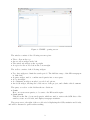
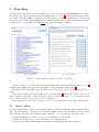
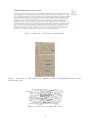
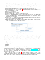
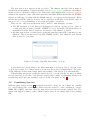
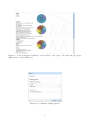
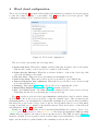
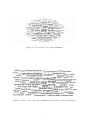
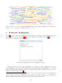
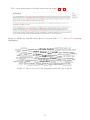
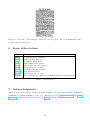
WAHSP
End-user Manual
Fons Laan
Informatics Institute
University of Amsterdam
Science Park 904
1098 XH Amsterdam
version 0·2·2
8 Jun 2012
Contents
1 Introduction
1
2 User interface
1
3 Searching
3.1 Query editor . . . . . . . . . . . . . . . . . . . . . . . . . . . . . . . . . . . . . .
3.2 Combining Queries . . . . . . . . . . . . . . . . . . . . . . . . . . . . . . . . . .
3
3
6
4 Word cloud configuration
8
5 Sentiment highlighting
10
6 Some abbreviations
12
7 Acknowledgments
12
1
Introduction
In this document we will describe how to use the web application of the Clarin WAHSP project.
With your browser 1 you can find the application at http://dev.wahsp.nl.
WAHSP is a research tools for historians that uses the newspaper data of the Koninklijke
Bibliotheek as input material. One can search with single query terms or with combinations
thereof. Apart from showing the articles that match the query, the results can be visualized by
word clouds of single articles together with sentiment words highlighted, or by a word cloud of
the whole result set together with newspaper statistics derived from their metadata.
Additional information about the project can be obtained from the Biland CMS site
http://biland.nl, which is the successor of WAHSP.
2
User interface
In this section we will give an overview of the components of the user interface. After accessing
the WAHSP URL you will see the login window, see fig. 1. Just clicking the Login button makes
you a guest user, but WAHSP collaborators will use their own credentials. Notice that there is
only one guest account, so other guests can delete the queries that you —as a guest— saved.
Figure 1: Login window.
The WAHSP opening window is shown in fig. 2.
1
Internet Explorer may not work with WAHSP. Please use Google Chrome, a recent Firefox, Opera, ...
1
Figure 2: WAHSP opening screen.
The window consists of the following screen regions:
•
•
•
•
The toolbar at the top
An accordion widget at the left
The article tab widget at the top-right
A region for the word cloud at the bottom-right
The toolbar consists of the following widgets:
• Two date widgets to limit the search period. The full date range of the KB newspapers
is 1900–1945.
• A query widget, used to combine saved queries into a new query.
• A logout widget.
• A configuration widget, mostly for word cloud options.
• An about widget, showing the collaborators of the project, and a link to this document.
The query accordion on the left has the two divisions:
• Search
Here one creates new queries, to be sent to the KB search engine.
• Saved queries
This shows the list of your saved queries, which are used to retrieve the OCR data of the
articles, create word clouds, and display newspaper statistics.
The screen area to the right of the accordion is for displaying the OCR, statistics and clouds,
and will be discussed together with searching.
2
3
Searching
A trivial way to search is by using a single query word. Say, we type vliegenzwam in the textline
area in the accordion, and then click the Seach button; see fig. 3a. It shows that 141 articles
are found. The first chunk is displayed with their titles in blue and underlined. Underneath
the title is some additional information: the newspaper title, article date, and newspaper ‘type’
(country-wide, or regional). Clicking next gives the next chunk of articles.
(a) Search panel
(b) Saved queries
Figure 3: Search and Saved queries in the accordion.
When you click one of the article titles, its OCR text is shown in the Text tab, see fig. 4.
Clicking the Original tab shows the scan image of the newspaper article (fig. 5).
The third tab View at KB opens the KB search engine page in a new browser window (or
tab).
The corresponding word cloud of the article is shown in fig. 6. The used font size of the words
is the graphical equivalent of their frequency in the document. Words of too low frequency may
not be shown, and in general ‘noise’ is also suppressed.
Inspecting the words in the cloud may lead one to make adaptations to the original query.
3.1
Query editor
Creating queries that consist of more than a single word is done with the built-in query editor.
The editor is easiest to explain by creating an example query. Let say that we create a new
query that we will later save with the name ‘luminal’. Proceed with the following steps:
• In the Search panel of the accordion, type luminal as search term.
• Click on the tiny arrow on the right half of the Search button.
• Click on the button Start search that appeared underneath the Search button.
3
Figure 4: OCR text of a KB article in the Text tab.
Figure 5: Scan image of a KB article in the Original tab. The word vliegenzwam is blue because
that was the query.
Figure 6: Word cloud of a single KB article.
4
• Below the text widget (that now contains (cql.serverChoice exact ”luminal”)) there is a
new button with text luminal. Click on its arrow at the right side.
• You will see a new frame with several buttons and other widgets. Click on the button
Make word list.
• Next to Word list: luminal there is a tiny icon of the inline editbox, click on it.
• Type chloral in the text region (see fig. 7) en then press Enter. Next to luminal we now
also see chloral in the word list.
• Once more press the icon.
• Type wekaminen and press Enter.
• Click the Search button, which shows the found records.
• Then go to Saved queries in the accordion and at Type query title here. type luminal, and
click the Save query button. Then luminal is displayed as the new saved query (unless
that name is already taken).
• Click its first icon (with hover text Create basis lexicon: luminal). This loads the OCR
data of all the luminal articles from the KB.
• When the loading is done, click the second icon Apply query: luminal. That creates the
cloud of the luminal articles, plus some statistics.
Figure 7: Query editor.
The Saved queries panel shows the query titles, their article count, and the creation date of
the queries that you have saved. If the article count is zero, either you have not loaded the KB
data, or there just is no loadable data, because your query did not yield a single hit. To the
right of each query are four small icons. When you move your mouse over them, you will see
their hover text:
•
•
•
•
Create basis lexicon
Apply query
Modify
Delete
After you saved a new query, it is important to realize that you cannot show the word cloud
of those articles together yet, because the OCR text of all articles has to be fetched from the
KB, and be pre-processed by our xTAS (Text Analysis Service), see http://xtas.net. That
will be accomplished by clicking the first of the four icons. When the query yielded many
articles it is time for coffee.
After a while the loading is done (fig. 8), and the number of articles is shown. Please
remember this number for moment. What is actually done, is that WAHSP finished delegating
all the hard work to a bunch of helper processes. And they may need a bit more time.
5
The new lexicon now appears in the accordion. The number after the lexicon name in
brackets shows the number of articles available. If it is a single number identical to the number
mentioned before, then the loading is done. But it may easily happen that you see two numbers
which are the separate counts of the article metadata and ORC. It likely means that the WAHSP
helpers are still busy. You may click the Refresh button to see if progress is being made. When
the metada and OCR counts are non-zero the second tiny icon will have been enabled, and you
can proceed to look at preliminary word clouds and graphs of statistics.
There are two other reasons that may lead to article counts changing over time.
• The KB digitization of the historical newspapers is still an ongoing process. Once in
a while new data is made available. WAHSP does not check this, but when when you
manually reload the data you may see an increase of the number of articles.
• Another issue is that over time (days, weeks) the metadata and OCR count may become
different. This is an unresolved bug (like WAHSP itself?). Reloading the data will fix
this, at least for some time.
Figure 8: Loading of the KB data seems to be done.
So the article set corresponding to the query must first be loaded in order to view the cloud
of all words together. For a single article you can view the word cloud immediately. The cause
of this difference is that with a single article the fetching of the data is done automatically.
When fetching and pre-processing the articles is done, you can click the second icon, which
now produces the word cloud of all articles together (after a while, accumulating all the word
frequencies), and some basic statistics of the lot in the text panel, see fig. 9.
3.2
Combining Queries
With the query widget (see fig. 10, reachable from the toolbar) one can combine two existing
(i.e. saved) queries into a new query. First select the desired boolean combination operator
(AND, OR or NOT), and then select the first and second query from the available list. The
widget will suggest a name for the combined query, but you can change that before clicking
OK.
6
Figure 9: Some newspaper statistics corresponding to the query. Hovering the pie pieces
displays the corresponding text.
Figure 10: Combining existing queries.
7
4
Word cloud configuration
The word cloud in fig. 6 was made with default cloud parameters, but there are several options
to tune the result according to your wishes. Fig. 11 shows the word cloud options. This
configuration widget can be opened from the toolbar.
Figure 11: Word cloud configuration.
The word cloud options have the following effect:
• Require fresh cloud. This adds a dummy variable with random value to the cloud request.
This should convince your browser not to return a cached result.
• Reduce font size differences. When the word sizes decline too fast at the cloud edge, this
option should improve the result.
• Font scale factor. This scale factor determines the maximum font size.
• Remove stop words. This removes short words, as specified by a pre-defined list.
• Remove words shorter that 3 characters. When the stop word list does not block enough
noise, this will filter more.
• Stemming. This applies stemming to the words before computing the cloud.
• Named-Entity Recognition. This applies NER, currently a bit slow.
• Max. # of words in cloud. The number of words returned by the server can be very big.
Truncating the list before generating the cloud speeds it up.
Fig. 12 shows the word cloud of the query wekaminen, which yields (only) 11 articles. Often,
as in this case, the cloud does not properly occupy the available space. One can increase the
maximum number of words displayed to remedy this, assuming more words are indeed available.
But when the words at the border of the cloud are already small, that does not help much,
because words that are too small become invisible anyway. Then it is better to reduce the font
size differences, see fig. 13 for the result.
Finally, fig. 14 shows the same word cloud with Named-Entity Recognition. Used colors:
locations, persons, organizations, and miscellaneous. The latter means that the NER algorithm
‘thinks’ these are entities, but cannot be more specific about it. The NER we used is Stanford,
trained for Dutch. It is not perfect, but it is better than several alternatives. Notice that the
figure only shows the recognized entities, the remaining words are left out.
8
Figure 12: Word cloud of the query wekaminen.
Figure 13: Word cloud of the query wekaminen with reduced font size differences.
9
Figure 14: Word cloud of the query wekaminen with Stanford Named-Entity Recognition. Used
colors: locations, persons, organizations and miscellaneous.
5
Sentiment highlighting
In fig. 4 we showed the plain OCR text of an article. After turning on the sentiment option in
the configuration widget (see fig. 15), the article OCR looks as depicted in fig. 16, with positive
and negative sentiment words highlighted.
Figure 15: Sentiment option in configuration widget.
This is an article from the query monstrum. (Now that we speak of sentiment, should we
add monstrum to the red list?) The figure also shows that what is highlighted are not whole
words, but substrings, which may lead to curious mistakes. And the OCR will never be perfect,
which clearly affects the results2 .
2
Apart from OCR mistakes, there is a second shortcoming in the data. The semi-automatic segmentation
of the newspaper scans into individual articles is not perfect either, leading to numerous ‘oversegmentation’:
‘articles’ consisting of just their title, their body text having been delegated to the next article. The current
settings of the KB search engine imply that short articles come first in the result list.
10
The corresponding article cloud and scan are shown in figs. 17 and 18.
Figure 16: OCR text of the KB article Een kat in kapok! with positive and negative sentiment
highlighting.
Figure 17: The word cloud of the newspaper article Een kat in kapok!.
11
Figure 18: The scan of the newspaper article Een kat in kapok!. The word monstrum is blue,
because that was the query.
6
Some abbreviations
Abbr.
Meaning
CQL
GUI
KB
NER
OCR
SRU
XML
xTAS
URL
WAHSP
Contextual Query Language
Graphical User Interface
Koninklijke Bibliotheek
Named-Entity Recognition
Optical Character Recognition
Search/Retrieval via URL
eXtensible Markup Language
Text Analysis Service
Uniform Resource Locator
Web Application for Historical Sentiment mining in Public media
Table 1: Abbreviations.
7
Acknowledgments
Apart from having received comments from my WAHSP colleagues (Daan Odijk, Stephen
Snelders & Toine Pieters), I also got contributions from José de Kruijf and Jaap
Verheul of Utrecht University, and my new Biland colleague Pim Huijnen.
12