Download Report - Image Group

Automation of measurements of pH levels
in cancer cells
Casper Petersen
Exam Number 8
011183-1629
Supervisors
Associate Professor
Ph.D Student
Jon Sporring
Melanie Ganz
Submitted in partial fulfilment of the requirements
of the degree of Master of Computer Science
April 16, 2010
Department of Computer Science
University of Copenhagen
Abstract
Measurements of pH levels in acidic cellular compartments of cancer cells as a function of time,
is relevant in relation to the development of new drug delivery systems. The measurements are
calculated from images taken by nanoparticle sensors by performing a series of steps using the
popular open-source ImageJ Fiji software. In this report we present a simple application based
on this software. In contrast to Fiji the application encapsulates only essential functionality as
specified by a researcher at RISØ National Laboratory for Sustainable Energy. Through a series
of meetings with the researcher and by using an iterative design cycle coupled with participatory
design and discount usability testing an interface was designed, developed and tested. The result is
a functioning application which allows the researcher to carry out the same tasks as in ImageJ Fiji
faster as a number of steps have been automated while also being able of performing user-specific
pH calculations.
Contents
1 Introduction
1
Problem description . . . . . . . . . . . . . . . . . . . . . . . . . . . . . . . . . . .
1
1
2 Mathematical Morphology
1
Introduction and Background Subtraction . . . . . . . . . . . . . . . . . . . . . . .
2
Segmentation Algorithms . . . . . . . . . . . . . . . . . . . . . . . . . . . . . . . .
2.1
Morphologic Watershed . . . . . . . . . . . . . . . . . . . . . . . . . . . . .
3
3
5
8
3 Application outline
1
ImageJ Fiji . . . . . . . . . . . . . . . . . . . . . . . . . . . . . . . . . . . . . . . .
2
The Application . . . . . . . . . . . . . . . . . . . . . . . . . . . . . . . . . . . . . .
11
11
11
4 User-Interface Development and Testing
1
Designing the User Interface . . . . .
2
Usability Testing and Results . . . . .
2.1
Usability Testing . . . . . . .
2.2
Carrying Out Usability Testing
2.3
Result of User Testing . . . .
.
.
.
.
.
13
13
15
15
17
17
5 Discussion, Conclusion and Future Work
1
Discussion . . . . . . . . . . . . . . . . . . . . . . . . . . . . . . . . . . . . . . . . .
2
Conclusion and Future Work . . . . . . . . . . . . . . . . . . . . . . . . . . . . . . .
19
19
20
6 User manual
A
User guide to BIO-GUI v.1A . . . . . . . . . . . . . . . . . . . . . . . . . . . . . . .
22
22
.
.
.
.
.
.
.
.
.
.
.
.
.
.
.
.
.
.
.
.
.
.
.
.
.
.
.
.
.
.
.
.
.
.
.
.
.
.
.
.
.
.
.
.
.
.
.
.
.
.
.
.
.
.
.
.
.
.
.
.
.
.
.
.
.
.
.
.
.
.
.
.
.
.
.
.
.
.
.
.
.
.
.
.
.
.
.
.
.
.
.
.
.
.
.
.
.
.
.
.
.
.
.
.
.
.
.
.
.
.
.
.
.
.
.
.
.
.
.
.
.
.
.
.
.
i
List of Figures
1.1 Steps required to be carried out by the researcher to get intermediate results from
ImageJ Fiji. . . . . . . . . . . . . . . . . . . . . . . . . . . . . . . . . . . . . . . . .
1.2 Example of applying the steps from table 1.1 in ImageJ Fiji to find and calculate
intermediate values to be used in pH calculations. From top to bottom, left to
right: ImageJ Fiji toolbar, red flourophores image, green flourophores image, R1,
intermediate values, ROI manager. The many spots seen on the R1 image are the
ROIs plotted on the image. The intermediate values are calculated on basis of ROI
attributed such as area, mean and standard deviation. . . . . . . . . . . . . . . . .
1
2
2.1 Dilation (middle) and erosion (right) of A by B (left). The structure element B is
shown with its origin as a black dot. The dashed line outlines the original object. .
2.2 Image (left) the opening of the image with a disk of size 5 (middle) and the opening
subtracted from the original image (right). . . . . . . . . . . . . . . . . . . . . . . .
2.3 Derivatives of an image. Original image (left), the (skewed) edge separating the
light and dark side (mid-left), first-order derivatives (mid-right) and second-order
derivatives (right). . . . . . . . . . . . . . . . . . . . . . . . . . . . . . . . . . . . .
2.4 Original image (left), region-growing from the center pixel (middle), and the impact
noise has on the image and the resulting region-growing (right). Image is taken
from http://read.pudn.com/ . . . . . . . . . . . . . . . . . . . . . . . . . . . . .
2.5 Left: Active contours. A region is specified around the target object and the snake
shrink-wraps around it. Right: Level set method. Top row shows the surface we
are interested in. In the bottom row the red structure is the graph of the level set
function and the blue square is the x-y plane moving up and down the z-axis of the
structure. Images are taken from Kass et al. [7] and http://en.wikipedia.org/
wiki/Level_set_method . . . . . . . . . . . . . . . . . . . . . . . . . . . . . . . .
2.6 Preliminaries of the watershed algorithm. A topological map with its contours
shown on the x-y plane. Red colors indicates higher points and peaks, where blue
colors identify lower points and valleys. . . . . . . . . . . . . . . . . . . . . . . . .
2.7 Two catchment basins at time t = n − 1 shown in white (left). Result of dilating
each basin (right) with a 3 × 3 structure element (not shown) with overlap shown
in gray at time t = n. . . . . . . . . . . . . . . . . . . . . . . . . . . . . . . . . . . .
9
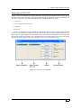
3.1 Screenshot of developed application after carrying out the steps from figure 1.1. The
ROI’s are shown on a high-precision (32-bit) image as requested by the user. The
calculations table contain the area of each ROI, mean and standard deviation of the
green and red fluorophores image, the ratio of the green mean to the red, and the
pH for each ROI. The ROI manager is intentionally not included. . . . . . . . . . .
12
4
5
5
7
8
9
4.1 The iterative design paradigm. Image is taken from http://www.naviscent.com/
en/i/ . . . . . . . . . . . . . . . . . . . . . . . . . . . . . . . . . . . . . . . . . . .
4.2 Learning curve for a novice and expert user in terms of efficiency as a function of
time. Image is taken from Nielsen [12]. . . . . . . . . . . . . . . . . . . . . . . . .
1
13
17
A screenshot of the BIO-GUI . . . . . . . . . . . . . . . . . . . . . . . . . . . . . . .
28
ii
List of Tables
3.1 Summarized overview of the most important objects in the application. . . . . . . .
12
4.1
4.2
4.3
4.4
.
.
.
.
14
16
18
18
5.1 User suggestions to the next version of the application . . . . . . . . . . . . . . . .
20
1
27
Problems using ImageJ Fiji. . . . . . . . . . . . . . . . . . . . . .
MoSCoW list of user requirements . . . . . . . . . . . . . . . . .
Usability problems identified during usability testing. . . . . . . .
User-specified positive and negative comments of the application
.
.
.
.
.
.
.
.
.
.
.
.
.
.
.
.
.
.
.
.
.
.
.
.
.
.
.
.
.
.
.
.
.
.
.
.
Common mistakes and their solution . . . . . . . . . . . . . . . . . . . . . . . . . .
iii
1
Introduction
1 Problem description
At RISØ National laboratory a researcher, as part of her work, is using fluorophores images obtained from two nanoparticle sensors in order to calculate pH levels of acidic cellular compartments
in cancer cells. Fluorophores images are the molecule components in a cell that emits light with
a specific wavelength when excited with light of a shorter wavelength. One of the flourophores
images (green) is sensitive to the pH of its surroundings and the intensity of the emitted light
changes with the pH. The other image (red) is pH insensitive and is used as a reference. A pair of
these flourophores images are called an image-slice, and it is on the basis of each such image-slice
the researcher is measuring the pH level.
Until the start of this project the pH measurement were not calculated using ImageJ Fiji. Rather
the researcher would obtain intermediate results using ImageJ Fiji, and calculation of the actual
pH measurements was done in a post-processing step. These intermediate results comes from a
table corresponding to a number of regions-of-interest (ROIs) calculated using ImageJ Fiji, with
each ROI having certain associated attributes such as area, mean and standard deviation, and it is
the value of these attributes which are then used to calculate pH levels in the post-processing step
using third-party software. In order to get these intermediate results the researcher is manually
required to perform the steps shown in figure 1.1, with a typical result of performing these steps
shown in figure 1.2.
Add the two
flourophores images
creating image R1
Subtract
background on R1
Adjust brightness
and/or contrast on
R1
Set threshold on
R1
Analyze particles
on R1
Run watershed on
R1
Invert R1
Figure 1.1: Steps required to be carried out by the researcher to get intermediate results from ImageJ Fiji.
Although figure 1.1 looks simple the components which is used to access this functionality is
scattered throughout the ImageJ Fiji toolbar making navigation slow and time-consuming. On top
of that these steps must be carried out for each image-slice, and as there can be arbitrarily many
of them this quickly begins to have an impact on number of image-slices the researcher can hope
to analyze, which is commonly referred to as throughput.
Throughput is classic problem in computer science originating in communication networks,
but is a term widely used to describe any problem dealing with a performance bottleneck. The
obvious solution to such a problem is to remove the components constraining the throughput, and
this is most easily done by designing and developing a new application which does exactly that.
1
1. PROBLEM DESCRIPTION
Figure 1.2: Example of applying the steps from table 1.1 in ImageJ Fiji to find and calculate intermediate
values to be used in pH calculations. From top to bottom, left to right: ImageJ Fiji toolbar, red
flourophores image, green flourophores image, R1, intermediate values, ROI manager. The many
spots seen on the R1 image are the ROIs plotted on the image. The intermediate values are
calculated on basis of ROI attributed such as area, mean and standard deviation.
First of all the application should remove the third-party software dependency for carrying out the
pH calculations by simply including the calculations in the code. Secondly the application should
provide the same functionality as underlying the steps in table 1.1 which can be done by using
ImageJ Fiji as the engine. Thirdly the navigation issues can be solved by designing an interface
which provides the user with instant access to the steps from table 1.1, and finally throughput can
be further improved by automating steps which does not explicitly require user interaction.
The proposed application will hence become a shell encapsulating only the necessary functionality in a simple easy-navigational design which automates steps considered non-essential. The
project is ideally suited for computer science students as a thorough understanding of programming and software designing are required to solve the problem.
The following report will describe the proposed application by dealing with the theory behind
some of the functionality described in the steps from table 1.1, before moving on to the application
itself and finally the design, development and testing of the application.
2
2
Mathematical Morphology
1 Introduction and Background Subtraction
The main idea behind mathematical morphology is to analyze the shape of an object in an image by probing the image with a geometric structure, typically called the structuring element,
such as a disc, a square, a line segment and the likes. The basic building block of morphology is set theory. The combination of fundamental set-operators like union, intersection, complement lead to powerful morphological operators that allow for object detection. The purpose of this section is to shed light on the morphological operations used in the implementation of our application. The reader can find an introduction to set-theory and the notation at
http://en.wikibooks.org/wiki/Set_Theory/Sets.
The two most fundamental primitive operators used in morphology are dilation and erosion.
Despite most other morphological procedures have their offset in these two operators, two additional operators not typically found in set theory must first be defined before dilation and erosion
are introduced. The two operators required are reflection and translation, and following the notation of [4] the reflection of a set B is given as
B̂ = {w|w = −b ∀b ∈ B}
2.1 and the translation of a set B by a point z = (z1 , z2 ) is given as
(B)z = {c|c = b + z ∀b ∈ B}
2.2 With these two operators the dilation of A with a structuring element B in a Euclidian 2D space
is given as
A ⊕ B = {z|(B̂)z ∩ A ⊆ A}
2.3 That is to say that the dilation is the result of reflecting around the origin of the structuring
element followed by translating the element around the object where the intersection of the element with the object is non-empty (similar to Minkowski-addition, see [3]). In a similar manner
the erosion of A by B is
A B = {z|(B)z ⊆ A}
2.4 which is to say that a point is contained in the erosion if and only if following translation by a point
z, B is still a subset of A. The structuring element B is often chosen to be a disc of size 3 × 3, but
many shapes exist for different purposes.
3
1. INTRODUCTION AND BACKGROUND SUBTRACTION
B
A
A B
A B
Figure 2.1: Dilation (middle) and erosion (right) of A by B (left). The structure element B is shown with
its origin as a black dot. The dashed line outlines the original object.
Although figure 2.1 shows these concepts, it may be difficult to understand how to use the
operators. To that end consider the dilation operator as an example. As long as the intersection
with the structuring element B is non-empty we ”grow” the object A by the structuring element
(with respect to its origin). Hence applying the dilation operator will close gaps between objects
with an intra-distance smaller than the structuring element.
The erosion operator can be thought of as the some-what opposite of dilation. If one thinks
of A in figure 2.1 as an object in an image, the erosion of an object with a structuring element
removes objects smaller than the size of the structuring element. As an example erosion is often
used as a pre-processing step in image analysis to remove gaussian, salt-and-pepper and speckle
noise.
The example given in figure 2.1 is the very basic application of two such fundamental operators. However as stated initially the power of set-theory allows new operators to emerge from
existing ones. In the case of dilation and erosion two new operators are called the opening
A ◦ B = (A B) ⊕ B
2.5 and closing
A • B = (A ⊕ B) B
2.6 and are simply combinations of the primitive operators introduced above. The aim for introducing
these operators is to develop an understanding of ImageJ Fijis subtract background routine.
The purpose of an opening is to correct the crude behavior of an erosion treating all foreground
pixels indiscriminately by applying dilation. The effect of an opening is to preserve foreground objects that have a similar shape to the structuring element, or that can completely contain the
structuring element, while eliminating all other regions of foreground pixels. The result of an
opening is thus dependent on the size and type of structure element. Choosing a structure element
that is different than the structures in the image will cause blurring, and choosing its size to be
larger than the largest object will remove the entire foreground.
The subtlety of this is that the subtraction of the opening from the original image will attenuate
the background intensities to a uniform level, from which subtleties can be enhanced using brightness and contrast settings. Background subtraction is illustrated in figure 2.2 on a typical image.
In the original image on the left in figure 2.2 the upper half has a bright background illumination whereas the lower half does not. In the opening of the image the shape of the structure
element can vaguely be detected, whereas the outlines of the objects in the image can be seen
quite clearly. Notice also how the choice of structure element has caused heavy blurring.
Finally the subtraction of the opening shows the attenuating background, but an artifact is
also present as many of the rice grains have become darker. With the relatively small structure
element the shape of the grains are traced as the structure element is matched, and the intensity
is changed depending on how well the structure matches (i.e. less blurring occurs). Therefore the
4
2. SEGMENTATION ALGORITHMS
Image
Opening
Image - opening
Figure 2.2: Image (left) the opening of the image with a disk of size 5 (middle) and the opening subtracted
from the original image (right).
brighter the grains are in the opening, the more they suffer from artifacts in the subtraction. These
effects can be greatly reduced by using a structure element (a) of larger size or (b) with a better
object-matching shape.
2 Segmentation Algorithms
The purpose of a segmentation algorithm is to find connected regions within an image with a specific property such as color or intensity, or a relationship between pixels, that is, a pattern. Such
algorithms are usually an intermediate step of image analysis and simplifies the representation of
the image often with the intention of making further processing easier. The purpose of this section
is to present an overview over the various segmentation algorithms available highlighting their
strengths and weaknesses, and ending with an in-depth look at the Watershed algorithm used in
the implementation and the reasoning behind choosing it.
Some of the earliest segmentation algorithms were based on edge detection. A number of edge
detectors exists such as f.x. Canny[1] and Sobel. An edge can be defined as a connected set of
pixels that lie on the boundary between two regions [4]. Thus to be able to distinguish between an
edge and its regions some property capable of being measured must be available. For the purpose
of gray-tone images, the intensities are the most frequent property, and the use of edge detection
in gray-scale images often relies on identifying sharp discontinuities in these intensity values. For
that purpose first- and second-order derivatives are the mathematical tools most commonly used,
and figure 2.3 will serve as the basis for explaining their use.
Original image
∂f
∂x
Edge in f (x, y)
∂f
∂x2
of f (x, y)
1.2
1.2
1.2
1
1
1
0.8
0.8
0.8
0.6
0.6
0.6
0.4
0.4
0.4
0.2
0.2
0.2
0
0
0
−0.2
0
20
40
−0.2
0
20
40
−0.2
0
of f (x, y)
20
40
Figure 2.3: Derivatives of an image. Original image (left), the (skewed) edge separating the light and dark
side (mid-left), first-order derivatives (mid-right) and second-order derivatives (right).
5
2. SEGMENTATION ALGORITHMS
First-order derivatives on a 2D image f (x, y) are defined as
∂f ∂f
∇f (x, y) =
,
∂x ∂y
2.7 Referring to figure 2.3 a detected edge in the original image (figure 2.3 mid-left) will in the firstorder derivatives manifest itself as positive at the point of transition in and out of the ramp [4],
whose size is directly related to the size of the derivative kernel. Looking at the points of transition
the line-segment connecting them has the same length as the slope in the original image. Using
this information the magnitude of the first-order derivative can therefore be used to determines
whether a given point is on a ramp or not.
Second-order derivatives on a 2D image f (x, y) are defined as
2
∂ f ∂2f
,
∇2 f (x, y) =
∂x2 ∂y 2
2.8 To detect edges one looks for zero-crossings i.e. places where the a transition goes from negative
to positive or positive to negative. The order of the transitions can reveal whether the edge is
going from dark to bright or vice-versa, and the line connecting the local minimum and maximum
will cross zero around its midpoint. As it was the case with the first-order derivatives the length
of the segment equals the length of the ramp in the original image with respect to the x-axis. In
figure 2.3 (right) the second-order derivative is shown for the original image. Notice that the segment connecting the local maximum and minimum is not completely straight as the ramp in the
original image has a non-binary transition.
Although the example given is purely 1D extending to 2D is only a matter of defining an edge
perpendicular to the edge direction at any given point and interpreting the results from the explanation above [4]. For the ideal discontinuity-example in figure 2.3 the derivative-based edgedetectors work very well. Unfortunately when noise is introduced the methods fall apart. An
illustrative example can be found in [4]. The main point to be made is that noise makes detecting
an edge, using the approach outlined above, very difficult in either derivative. The problem with
the noise could be fixed by applying an appropriate smoothing filter f.x. a gaussian kernel. However for the purpose of the application smearing the particles is not an option as it would render
the pH-calculations useless.
Another approach to segmentation are the region-based algorithms. The objectives for these
algorithms are to
• Produce regions that are as large as possible (that is produce as few regions as possible).
• Produce coherent regions, but allow some flexibility for variation within the region.
Here the inherent trade-off becomes visible. If we want large regions we must allow more flexibility which could cross multiple object boundaries and ”leak” across what should have a boundary.
This can be corrected by allowing less flexibility but in turns we risk over-segmentation i.e. locating objects much smaller than than actual objects.
The region-based techniques can be further divided into a number of subclasses, and of these
the most commonly used are the region-growing algorithms. For such an algorithm suppose you
start with a single pixel p as a seed point and we wish to grow, from that pixel, a connected region
based on some property. Define a binary similarity function f (p, q) → x that returns a 1 if the
value of the image at point q is similar to the value at point q within a certain threshold T , and 0
otherwise. Starting from p the neighboring pixels can now be examined. If f (p, q) > T then q can
be added to p’s region and q’s neighbors can now also be examined. Continuing recursively in this
manner inevitably yields a region.
6
2. SEGMENTATION ALGORITHMS
There are however several issues to address. First, selecting a seed point is non-trivial as different seed points yields different results as the method is localized. Likewise using a non-adaptive
threshold could result in regions where the objects in the image are not entirely captured or grossly
over-represented. Finally choosing a similarity function could be anything from individual pixel
intensities, gradient information or even geometric properties.
These issues makes region-growing a difficult technique to apply and similar to the edge detection algorithms there is an inherent sensitivity to noise. An example is given in figure 2.4.
Comparing the middle image with the left the number of gray tones have been reduced as pixels
have been clumped together by their intensity as outlined above. However the image on the right
shows the over-segmentation occurring when noise is present in the image as there is a lot of regions no more than a few pixels wide with intensities below the threshold used.
Region growing
Original image
Region growing on noisy image
Figure 2.4: Original image (left), region-growing from the center pixel (middle), and the impact noise has
on the image and the resulting region-growing (right). Image is taken from http://read.pudn.
com/
The process outlined above will only detect one object and will only work if the image is not
too corrupted. One could select several seed points and carry out the procedure simultaneously,
but the problems described above would persist regardless. Also without a priori knowledge on
the amount of objects in the image it is impossible to detect all objects.
Introduced in 1987 active contour models [7], or snakes, represent object boundaries (or other
salient features) as parametric curves with an associated energy-function that is sought to be minimized. The main idea is that positioning a snake near an object will cause the snake to deform
(shrink-wrap) to match local minima on the parametric curve. Thus to find the best fit we must
minimize the snakes energy. Mathematically the snakes energy function is written as
Esnake =
Z
0
1
(Einternal + Eimage + Eexternal v (i))
2.9 where the snake is parametrically defined as v(i) = (x(i), y(i)), Einternal is internal energy caused
by bending and stretching, Eimage is a measure of the attraction of image features and Eexternal
is a measure of external constrains either from higher level shape information or user applied energy [7]. The energy functions are defined cleverly such that the snakes final position will be at
an energy minimum. For example the external energy function makes use of the negative image
gradient which takes on smaller values at the features of interest such as boundaries. The remaining energy functions have characteristics which also serve to minimize the snakes complete energy
function at object boundaries. An example of active contours is shown on the left in figure 2.5.
Although resistent to noise there are weaknesses in the active contour model. Convergence
relies heavily on the initial position of the snake(s), and the number of parameters in the energy
function makes the result extremely sensitive to small perturbations in the user-controlled variables. Also as the external force does not affect points far away from the boundary this makes
detecting concave boundaries difficult. Thirdly, as it was the case with the region-growing, a priori
knowledge of the number of objects we want to detect must be known, as snakes cannot be dis7
2. SEGMENTATION ALGORITHMS
Figure 2.5: Left: Active contours. A region is specified around the target object and the snake shrink-wraps
around it. Right: Level set method. Top row shows the surface we are interested in. In the
bottom row the red structure is the graph of the level set function and the blue square is the x-y
plane moving up and down the z-axis of the structure. Images are taken from Kass et al. [7] and
http://en.wikipedia.org/wiki/Level_set_method
continuous.
As the snake-approach is explicit in its parametric form it does not handle deformation very
well if it involves splitting or merging of parts/objects. To circumvent these problem the Eulerian
approach also called level-sets are introduced which handle topological changes naturally. The
level set method works by implicit tracking a surface that intersects the x-y plane which is called
the zero level set. The level set function can be visualized as a graph in 3D with the x-y plane
moving up and down the z-axis. Tracking the surface in this manner simply becomes a matter of
defining a function that given any point in the plane returns its height as this will only be positive
above the zero level set. The right part of figure 2.5 illustrates the above description. For the
purpose of segmentation the level set method would segment an image correctly. However the
method is not robust against gaps and suffers from various other deficiencies [19]. For example
it is very difficult to implement the method, and it requires finding an energy function which is
non-trivial.
2.1
Morphologic Watershed
The segmentation algorithms discussed so far have been based on (a) line detection, (b) regiongrowing and (c) implicit and explicit contour-tracking. Each of the methods suffers from various
drawbacks and no single method would segment a typical image properly. The purpose of this section is to analyze the morphological watershed algorithm, which embodies many of the strengths
of the algorithms discussed until now and typically results in a better segmentation [4].
In gray-scale mathematical morphology the watershed transform can be classified as a regionbased segmentation approach. The intuitive idea underlying this method comes from geography:
it is that of a landscape or topographic relief which is flooded by water, watersheds being the dividing lines of the domains of attraction of rain falling over the region. To better visualize this
consider the image shown in figure 2.7 which illustrates a topographic map of a terrain with the
x-y plane showing the contours.
The basic idea behind the watershed transformation is simple: After piercing holes in the
minima their basins (also called catchment basins) will fill up with water starting at these local
minima, and, at points where water coming from different basins would meet, dams are built.
When the water level has reached the highest peak in the landscape, the process is stopped.
The result is a landscape partitioned into regions or basins separated by dams, called watershed lines or simply watersheds. A nice animation of this conceptual idea can be found at http:
//cmm.ensmp.fr/~beucher/wtshed.html.
8
2. SEGMENTATION ALGORITHMS
Topographic map of a terrain
Peaks and valleys
5
0
−5
−10
3
2
1
2
0
0
−1
−2
y−axis
−3
−2
x−axis
Figure 2.6: Preliminaries of the watershed algorithm. A topological map with its contours shown on the x-y
plane. Red colors indicates higher points and peaks, where blue colors identify lower points and
valleys.
To understand the Watershed transformation the preliminary concept of a connected component, which has its origin in graph theory, is introduced. In graph theory a graph is called connected
if every pair of vertices are connected by a path. The connected components of the graph are the
equivalence classes of vertices under the transitive relation.
With that definition the flooded content of a catchment basin can be seen as a connected component as all points are connected to each other. Using this conceptualization two catchment
basins in the x-y plane are shown on the left in figure 2.7.
Two catchment basins (white) at time t = n − 1
Flooding at time t = n
Figure 2.7: Two catchment basins at time t = n − 1 shown in white (left). Result of dilating each basin
(right) with a 3 × 3 structure element (not shown) with overlap shown in gray at time t = n.
Flooding is modeled as region-growing from a local minima Mi , but the essential part of the
watershed algorithm is knowing when to build the dams. Dams should be build whenever an overflow is detected i.e. when water from different basins spill over into one another. The definition of
overflow follows immediately from the connected components. If an overflow is detected a merging of two, or more, connected components takes place and the cardinality of the set of minima
9
2. SEGMENTATION ALGORITHMS
in the topographic surface reduces. The spilling can only be a result of the water level rising in
adjacent local regions, and to that end the dilation introduced earlier is used to simulate the rising
water in a region by dilating the connected components. Figure 2.7 illustrates this concept. On the
left two connected components are shown at time t = n − 1. The dilation operation that caused
these components to appear did not trigger an overflow and as such no merging took place. At
time t = n, shown on the right in figure 2.7, the water has risen due to another dilation and caused
the two components to become a single connected component. Thus at time t = n it becomes necessary to construct a dam.
A few conditions on the structure element used in the dilation is necessary. From [4] we know
that the dilation by a structure element (a) must be constrained to the outline of the boundary of
the component resulting from the flooding and (b) dilation cannot be performed on points that
would cause a merge. Thus from condition (b) the gray line in figure 2.7 indicates the points
where the dam must be build. The dams are built higher than highest point in the surface to prevent spilling as the flooding continues. As dams are built on all sides to isolate different regions
around the local minima they form connected components themselves, thus no discontinued watershed lines can occur.
Recursively executing the approach outlined above i.e. increasing the water level and building
dams constructs the unbroken segmentation lines, and all local minima eventually become walled
in on all sides.
So is the Watershed segmentation algorithm better? The result of the Watershed segmentation
is not locally dependant (using region-growing terminology), the seed points or local minima are
uniquely determined by the topographic nature. It is not discontinuous as each minima eventually gets walled in, it does not require complex energy functions and the inherent difficulties that
comes with them, and by introducing a pre-processing step involving markers one obtains a priori
knowledge which is what humans use every day to aid visual segmentation i.e. context. These
advantages means the Watershed segmentation is generally favored over the other algorithms discussed, but it is not perfect.
A severe drawback to the of watershed algorithm is oversegmentation i.e. relevant object contours are lost in a sea of irrelevant ones. This is partly caused by random noise, which gives rise to
additional local minima, such that many catchment basins are further subdivided, but irregularities
in the morphological gradient is also a cause of this phenomenon. An example of oversegmentation can be seen on the right in figure 2.4. To counter this one can use a variation of the watershed
algorithm which uses two kind of markers that limits the allowable number of regions in the image. Typically the image is smoothed to avoid the effects of noise and internal markers, which are
connected components associated with objects, are identified and used as local minima. The watershed algorithm is then run using only these minima as input. The watershedlines resulting are,
in this context, known as the external markers which segments the image into regions containing
only one internal marker. It is worth noting that the applying the Watershed algorithm globally
is the same as doing it locally for each minima as the watershedlines, and hence the result, will
remain unchanged.
10
3
Application outline
While the previous chapter dealt with a very specific aspect of some of the methods used in the
application, the purpose of this chapter is to briefly outline the application by introducing the
computational core of the application itself ImageJ Fiji and afterwards introducing the application
itself.
1 ImageJ Fiji
ImageJ Fiji is an open-source application distributed under the GNU license and is developed and
maintained exclusively for the purpose of medical imaging. Fiji (Fiji Is Just ImageJ) is a distribution based on the popular ImageJ which is a public domain Java image processing program
inspired by NIH Image for Macintosh. ImageJ was designed with an open architecture that provides extensibility via Java plugins. Custom acquisition, analysis and processing plugins can be
developed using ImageJ’s built in editor and Java compiler. More extensive customization can be
accomplished by user-written plugins which then augments the program and makes it possible to
solve many image processing and/or analysis problem.
Choosing Fiji as an engine for the application was convenient as the researcher already used
the program and was therefore familiar with the functions included in the developed interface.
This choice somewhat restricts the application to be written in Java as well though any software
capable of using the Java virtual machine could be made to work.
2 The Application
The application was developed using Java 1.6. Java is an object-oriented language meaning that
by using the language the world is perceived as containing objects and these objects can be interacted with through the use of functions inside the object. For example one can think of a drawer
as an object with functions such as open and close.
The object-view allows you to create modular programs and reusable code through inheritance
so emphasis is on data rather than procedure. The natural partitioning means the architecture
is straight-forward as an entire system can be build in smaller pieces. A more generalized look
on this natural partitioning results in a high-level architecture often used with graphical applications [15][14] called the Model-View-Control (abbreviated MVC). The purpose of the architecture
is to to group the objects according to their specific domain, with the model consists of a set of
classes which support the underlying problem, the viewer is the applications appearance to the
user on screen and the controller acts on input through the view. The most important objects
in each major component are referenced in table 3.1, and their UML diagrams can be found in
UML.rar at http://www.nonplayercharacter.dk/Project/B3/appendices.rar.
The application allows the user to manually carry out the steps from table 1.1 with the exception of subtract background (this was found to be an error and have since been fixed), image
11
2. THE APPLICATION
Object name
Model.java
Membership
Model
Viewer.java
Viewer
Control.java
Control
Calculations.java
Control
Summary
Contains the setters and getters required for
interaction between the the main objects.
Constructs the graphic user interface, and
adds listeners.
Acts on input from the graphical user interface, and reflect changes based on these in the
viewer. Contains majority of the control logic
extracted from the model.
Controls all calls to ImageJ Fiji as well as loading data, and all processing.
Table 3.1: Summarized overview of the most important objects in the application.
invert and watershed. After carrying out the final step from table 1.1 the user will be presented
with a 32-bit image where identified regions-of-interest (ROIs) are displayed. The ROIs will be
accompanied by a spreadsheet which contains the area, ratio, mean, standard deviation and pH
level for each such ROI calculated on the red and green fluorophores image associated with the
selected image-slice. pH calculations were done based on user-provided formulas. Furthermore
the application allows for batch-processing and has the user-manual built into it for easy reference.
A screenshot of the developed application can be seen in figure 3.1.
Figure 3.1: Screenshot of developed application after carrying out the steps from figure 1.1. The ROI’s are
shown on a high-precision (32-bit) image as requested by the user. The calculations table contain
the area of each ROI, mean and standard deviation of the green and red fluorophores image, the
ratio of the green mean to the red, and the pH for each ROI. The ROI manager is intentionally
not included.
Internal testing was carried out during development and a list of known bugs can be found at
http://www.nonplayercharacter.dk/Project/B3/appendices.rar where the source-code and
user-manual is also found.
12
4
User-Interface Development and Testing
The previous chapters have dealt with the more mathematical and technical aspects of the project,
all transparent to the user. In this section we turn to the focus point of the assignment: the
development and testing of a user interface capable of supporting the researcher in her everyday
work whilst improving efficiency through automation. First the theoretical foundation of the design
will be discussed, specifically the design paradigm and the techniques used. The second part will
center around how the testing of the user-interface was planned, how it was carried out and what
the results were.
1 Designing the User Interface
Following Nielsen [10] the iterative development
paradigm was chosen (depicted in figure 4.1) for two
main reasons. Firstly it is a well-established and recognized method as it is impossible to design a user-interface
which does not have any usability problems the first time.
The purpose of the paradigm is to identify usability problems and refine them iteratively. A completely iteration
in the paradigm allows the designer to (a) draft a design,
(b) create a prototype and (c) evaluate the prototype.
Ideally this is repeated until no further usability problems are found, though this is rarely, if ever, the case in
practice. Secondly the paradigm explicitly involves eval- Figure 4.1: The iterative design paradigm.
Image is taken from http://
uation which requires an assessment of a product in this
www.naviscent.com/en/i/
case the application developed. In this project the evaluation will be carried out by the researcher who is the
intended end-user of the application. As time constrains the number of iterations which can be
carried out, the evaluation will result in an acceptance or rejection of the entire application, and
since the application cannot be evaluated without a user-interface this forces the user-interface to
be a pivoting element in the project.
The purpose of a user interface is to support a user in communicating with a system for the
purpose of accomplishing certain goals [2]. In order to accomplish said goals with the user interface it becomes crucial to understand the user. This is referred to as taking a human-centered
approach [2] and is about
• Understanding what the user would want to do, rather than what technology can do and
• Involving people in the design process
These points fit well into the iterative paradigm as understanding and involving the user should
reduce the number of usability-problems.
Understanding the user is typically carried out through requirements analysis [2]. This type of
analysis is centered around understanding what people do, or might want to do, and about any
13
1. DESIGNING THE USER INTERFACE
problems they have with the current system. Obtaining this information and encapsulating it in
the design is therefore the first step in reducing possible usability problems.
A requirement is something a product must do, or a quality the product must have [16], and
these requirements were obtained through user-stories and interviews in order to understand the
problem. To this end one out of total three meetings was scheduled early in the course of the
project. The purpose of the first meeting was to get the program demonstrated by the user as she
carried out a typical task, while the user would talk about the problems she had with the software
during that time thus obtaining a user-story. Following the demonstration any misconceptions
or misunderstandings were corrected through an interview. At the end of the first meeting the
problems presented in table 4.1 had been found using meaning condensation [8] of the user-story.
The user agreed to these points being the main issues of the existing software.
Problem No.
1
2
3
Description
Lack of automating features makes analyzing the images
very slow.
The extensive interface makes navigation very timeconsuming. It should be more simplistic.
ImageJ Fiji did not support the calculation of pH values or
other types of calculations specified by the user.
Table 4.1: Problems using ImageJ Fiji.
The first two problems are correlated, but separable. Although both concern time, the first
problem is tied to functionality whereas the second is concerned with the design of the existing
software. The third one was specified by the user as a major problem. The combined solution
to the problems identified by the user in table 4.1 could therefore serve as an overall measure
of success against which the end-product could be compared. The problems in table 4.1 are too
general to design or develop a user-interface from, and as such they had to be partitioned into specific user requirements. Unfortunately no such list could be fully obtained during the first meeting
due to unforseen time-issues. However the user-story obtained combined with the problems from
table 4.1 did succeed in generating some requirements.
With only a partial requirements list from which to design from, the envisionment technique [2]
was adopted to externalize design ideas which would then be presented to the user. Using this technique allows the designer to compensate for the lack of requirements by conceptualizing what a
design might look like based on the information at hand, and designs are typically captured using sketches, artworks and the likes. However conceptualizing designs is not an easy task as it is
recognized that users operate with various mental models [13] which are the users’ mental image
of what the system looks like and what it can do. The user’s model does rarely, if ever, match the
one the designer has in mind, so some method had to be used to offset the conceptual differences,
thereby prevent mono-method bias (see [18]).
As involving the user to design the interface was stated to be a pivoting element in the project,
a technique called participatory design was chosen which aims to get the user involved as much as
possible in the entire design process. Using this technique offers the advantages that
• If the ideas presented to the user are not in line with the users mental model, the user can
become involved by making changes and/or adjustments to the design on the spot.
• The design can become the users own creation thus reflecting their mental model to the
designer. This can then be used in any future designs.
Thus envisionment can be a valid method when coupled with participatory design as the designs
conceptualized through envisionment can serve as a basis from which the user can create her own
14
2. USABILITY TESTING AND RESULTS
design by adding, removing, relocating or otherwise altering elements of the user-interface. Notice also that choosing participatory design as offset to envisionment takes care of the second point
from the list concerning the human-centered approach.
Applying envisionment resulted in a number of wireframes [5], which are computer-drawn
user interfaces representing the basic interface design including layout, simple buttons and plain
content, was created. Keeping the items from table 4.1 in mind the designs were kept as simple as
possible, including only the functionality in the form of buttons which, according to the designer,
could not be automated. The purpose of the wireframes were horizontal prototyping [2] where the
layout is explored instead of the functionality. The functionality would then be specified alongside
any design-changes in the participatory design phase. To give the user some variation to choose
from during this phase slightly different wireframes had been designed. These wireframes can be
found at http://www.nonplayercharacter.dk/Project/B3/appendices.rar.
With the wireframes designed the second meeting was scheduled. The purpose of this meeting
was to carry out the participatory design outlined above, and to get the points from table 4.1
partitioned into specific requirements from which the design and functionality could be refined.
After meeting the user, the purpose of the meeting was explained. The user was presented with
the wireframes in their printed form and was informed that she was not obligated to choose any of
the presented suggestions. Instead she was encouraged to cut/tear or otherwise alter the designs
as she saw fit until she was happy with a design. Surprisingly the user was completely indifferent
when it came to the design, and repeated attempts to try and get her to change the design proved
futile. The user simply specified she wanted a design which
• Contained a box with all the requested functionality readily available.
• Offered easy access to all time-series and image-slice in a loaded LIF file.
• Displayed the images in each image-slice separately.
Using that specification the user settled on the second design which can be seen in figure 3.1.
Returning to the requirements list the user was happy with the requirements conceptualized
which had been embodied in the wireframe she had selected. She was then presented with the
points from table 4.1 and was asked to break them down and specify them thereby creating a
complete requirements list. This generated quite a long list of requirements. Prioritizing these
requirements became a necessity to ensure that application design and development could finish
on time, and to that end the MoSCoW [2] (Must have, Should have, Could have, Would have) rules
were applied to list in joint conversation with the user. The resulting MoSCoW list is shown condensed in table 4.2.
With the requirements clarified and an accepted design, the third and final meeting was scheduled.
The purpose of this would be usability-testing of a functioning prototype capable of fulfilling as
many points from the MoSCoW list as possible.
2 Usability Testing and Results
Usability testing is the process of evaluating a product by testing it on its intended users. This
is the last step in the iterative paradigm and with only one user-testing session capable of being
carried out, this part would determine whether or not the project was a success. The purpose of
this section is to detail how the user-testing was carried out, and what the results were.
2.1
Usability Testing
There are many ways to carry out user-testing, but they all depend on the purpose of the product
plus the time and the number of users available. This has inherent trade-offs as
15
2. USABILITY TESTING AND RESULTS
Must have
All functionality she was using in ImageJ Fiji must be included in the
new interface. Otherwise the program cannot be used.
Should have
(a)Calculation of pH values for each region of interest (ROI) using
user-supplied formulas.
(b) Each LIF file saves for each image-slice the area, ratio, mean,
standard deviation and pH level for each (ROI) in a separate sheet in
a common XLS file.
(c) Displaying a high-precision (32-bit) image which is the result of
adding the first two images in each image-slice together.
Could have
pH calculations for each pixel rather than for each ROI.
Would have
Adding colormaps informing of the amount of overlap between image ROIs. Colormap should go from blue to red.
Table 4.2: MoSCoW list of user requirements
• Having many users test the product takes up more time
• Having many users test the product identifies more usability issues
The first point is self-explanatory, and the second stems from Nielsen [12]. Following his research
a minimum of 5 users, who are a part of the intended user-group, should test the application. As
this was not possible the it became a question about how to evaluate the user-interface with only
one user. This has several problems as identified by Nielsen [10][12], and no choice of methods
can offset these problems. Instead focus would be concentrated on trying to identify techniques
which would allow as many usability problems to be identified and reported. Choosing too rigid
techniques is not an option. For example a questionnaire allows little flexibility for the user to
voice an opinion about usability problems, as the questions can be confined to very specific parts
of the user interface where the experimenter believes the problems are located when they are in
fact not. Thus a set of more flexible techniques which also takes into account the time required to
prepare and carry out the testing would have to be selected.
A sensible compromise is the discount usability testing method [9] called Thinking Aloud introduced by Molich. Choosing this approach requires a minimum of time and users and novice
experimenters can apply the technique [6] with some success. The technique involves the user
telling the experimenter what he or she thinks as a response to using a system to solve a number of
tasks. By employing this part qualitative, part quantitative method it becomes possible to couple
user-input with the traditional attributes of usability testing given in Nielsen [11] which are (a)
learnability, (b) efficiency, (c) memorability, (d) errors and (e) subjective satisfaction.
Coupling the user-input and these attributes should provide an indication of whether the application has any serious usability issues. Of the points in the list, memorability can only be tested
after the user has tried the system once and was thus ignored. The remaining points would thus
form the basis of the usability-testing and would need to be operationalized.
Operationalizing learnability can, in the basic case, be accomplished by giving the user a number of tasks to carry out without any prior knowledge of the system, and then measuring how
many of these tasks are completed successfully. Errors were simply measured as tasks not completed within a reasonable time-frame. Although simple, the results can be very misleading because
they are determined solely on the difficulty and formulation of the tasks the user must complete.
In [9], Molich gives a number of guidelines which should be used to develop the tasks including
a pilot-testing to weed out initial problems / misconceptions. These guidelines were followed in
16
2. USABILITY TESTING AND RESULTS
order to develop the tasks, and pilot-testing being carried out by fellow student at DIKU.
Efficiency is coupled with learnability and is associated with the curve for a novice user shown
in figure 4.2. The coupling of the two attributes can be seen as learnability implies limited time
spent understanding and operating the application which, by the figure below, translates to improved efficiency. Measuring efficiency is thus equal to measuring time. However to make any
valid claims about efficiency solely based on time, a reference time must be established. This is
difficult as no other test subject from whom any benchmarks could be obtained was available. To
try and remedy this a 24 year old physics student with moderate computer knowledge was recruited and given a crash course in using ImageJ Fiji before carrying out the constructed tasks in
the developed user-interface which took her 16 minutes.
Figure 4.2: Learning curve for a novice and expert user in terms of efficiency as a function of time. Image is
taken from Nielsen [12].
The subjective satisfaction is the final point and can be thought of as a summarizer and a
specification. The method of choice here is the semi-structured interview [17] which allows the
interviewer to prepare a series of question concerning areas he/she finds important, but also allows
flexibility in case the user touches upon something not anticipated that must be followed through.
The purpose of the interview was to debrief the user with respect to the tasks the user carried out,
and at the same time determine whether the project was capable of being used by the user in her
work. This method off-sets the Thinking Aloud procedure as it gives the use a chance to repeat
and elaborate on specific topics.
2.2
Carrying Out Usability Testing
The usability testing would be the third and final meeting with the user, and would constitute the
evaluation of the iterative design cycle thus making or breaking the project. Following Molich [9]
the user was informed of the purpose of the current session, and it was emphasized that it was
not the user being tested but the application, and that the session would take approximately 30
minutes. Furthermore the user was told she could ask for help, but she could not be guaranteed an
answer. The team carrying out the usability testing was one person taking notes while the experimenter carried out the actual experiment as is advised [2]. To avoid bias due to the experimenter
also being the person designing the interface the impartial notes from the assistant wold be used
for analyzing the results, with the experimenters own notes used for verification.
2.3
Result of User Testing
Following the Thinking Aloud procedure the user was from time to time reminded to keep talking
as she used the application. The usability problems listed in table were all identified based on user
comments and the notes collected from the usability testing.
The second problem in table 4.3 is by far the most severe. The feature in question was the
subtract background function which in the first meeting had been conceptualized to be a static
variable, when in fact it was not. The user spent quite some time looking through the interface
17
2. USABILITY TESTING AND RESULTS
No.
1
Description
It was not clear to the user how to get images displayed
after opening an LIF file.
2
A feature which should not have been automated had been
which cause a lot of confusion.
3
The user could not figure out how to zoom.
4
It was unclear to the user whether it was necessary to close
images before opening a new LIF file, or choosing another
image-slice.
Table 4.3: Usability problems identified during usability testing.
while saying she did could not understand where the button to control this setting was located.
When informed the user immediately requested that function being incorporated into the interface.
The rest of the problems were figured out by the user without requesting any help or consulting
the user-manual.
Despite the usability problems the user never gave up using the interface. The user did not
get lost in the interface because of navigation issues, and the user did in fact only spent approximately 11 minutes solving the tasks which were almost 33% faster than the person who set the
benchmark did it in. As both the pilot user and the actual user had no previous experience with the
application this seems like a spurious event which could be corrected by recruiting more test-users.
Following up on the actual testing the interview sought to get the users opinion on key-issues
which would determine the success or failure of the application. The user was first asked to name,
if possible, up to the three most positive and negative things about the application. These are
shown in table 4.4.
No.
1
Positive comments
Simplistic design
Negative comments
Subtract background
must be manual
2
Accessible functionality
Could use more custom calculations
2
Custom pH calculations
functionality
Table 4.4: User-specified positive and negative comments of the application
The positive comments correlate well as solutions to the early generalized problems identified
in table 4.1. This is not surprising as the user selected a conceptualized design which had its origin in dealing with these problems specifically. The only missing from this table is and answer to
whether or not the level of automation was satisfactory. However when asked the user replied he
was indeed very happy with the current level of automation, when she didn’t take into consideration the subtract background functionality which had been automated. Combining the results from
first column of table 4.4 with that answer, a solution to the generalized problems from table 4.1
has been obtained. Unfortunately this is only half the answer, as it doesn’t tell whether the user
would actually to use the software as a substitute for ImageJ Fiji in her work. Fortunately when
the user was asked this question she replied that she would definitely use the software. Hereby the
goal of the project has been fulfilled.
18
5
Discussion, Conclusion and Future Work
1 Discussion
Despite the result indicating that the aim of the project has been fulfilled, there are several things
worth considering before drawing any meaningful conclusion. As the results are a direct consequence of the methods used the question of internal validity [18] is a very real threat as ruling out
rival hypothesis as plausible explanations for the results becomes difficult. As an example consider
the use of the iterative design paradigm. Although a valid choice, restricting its use to only one
iteration hampers the interface quality as a function of the number of design iterations as shown
in figure 1 in Nielsen [10]. Although vastly superior to carrying out no iterations, at best a single
iteration removes interaction flaws which was also the case from the usability testing in the project.
Combining this fact with the system being designed and developed for a single user and seeing as
this user will only identify up to about a third of the total number of usability issues [12], which
might not even be usability problems but a result of spurious behavior from the user, it is possible
that what the usability testing found was a result of a low-quality, poorly tested application.
Offsetting the possibility of a low-quality application can be done by using proven methods in
every step of the design. Unfortunately this standard was not met everywhere. Take the design of
the wire-frames as an example. Ideally paper prototypes which tests both design and functionality,
should have been designed and used for testing instead. The reason is that wire-frames are static
results of carrying out paper prototyping and seeing as this step was skipped, the conceptualization
of the designer guided the layout of the wire-frames. As a result the wire-frames came out very similar in appearance leaving the user with little to no intra wire-frame diversity to choose from, when
encouraged to personalize the interface through participatory design during the second meeting. It
is therefore likely that the indifference expressed by the user during participatory design is a result
of this shortcoming, thereby reducing the overall quality. The lack of rapid prototyping capabilities in Java were also a restraining factor with respect to the diversity of the wireframes. Initial
attempts to use MatLab to build the application proved unsuccessful.
Other cases similar to the one above can be made for other aspects of the project. In a similar
way the testing of the application could be improved by using appropriate techniques. Here the
problem is again the uniqueness of one user versus the generality of many when it comes to testing.
Having only one user means that in order to reduce variation in user response several iterations
of the design cycle would be needed whereas having a group of representative users could easier
get away with only one design iteration as the variation in the serious usability problems would
be small, thus attenuating spurious behavior. Determining the fluctuations from one user to another as they use the application is known as test-retest reliability [17], and it is an excellent way
to weed out spurious behavior when more users are available. For the single-user case it’s more
difficult, but one possibility would be to carry out more design iterations. Unfortunately trying to
investigate any of these matters was not possible within the time-frame of the project.
The problems outlined above does raise the question of why the software was approved by the
user. Although possible, it is hard to imagine that with only a single cycle of the design iteration
19
carried out there were no major usability problems remaining in the interface. Interestingly enough
when looking at the answers from the usability-testing, the user seemed more concerned with
adding an increasing number of custom calculations to the output rather than the design and
functionality of the program. Valuing computations over design lets the designer off the hook, but
in event that the user-interface must be extended there will not be a working foundation on which
to improve on. Again there was no time left to investigate this problem further.
2 Conclusion and Future Work
As ImageJ Fiji currently used by a researcher as RISØ National Laboratory to perform image analysis was becoming a performance bottleneck in her work life, a new application was developed.
The application provides a simple easy-to-navigate user-interface coupled with the functionality
the user is familiar with from ImageJ Fiji while also automating non-essential features to further
improve efficiency, and provides custom pH calculations. The design of the application was determined through requirements analysis extracted over two meetings with the end-user. Coupled with
envisionment, the requirements analysis spawned several design proposals which were attempted
refined through participatory design, eventually leading the user the select a design for the userinterface. With a design selected the MoSCoW rules were applied to the functionality requirements
which lead to working prototype of the application. Testing the application was done using Thinking Aloud and a semi-structured interview. The result of the Thinking Aloud test revealed that the
user had an easier time navigating the user-interface, with the interview confirming that she would
be able to carry out tasks faster and that, despite some usability problems, the user was overall
very happy with the application and would definitely use it in her work.
Future work with the application can be based on the requirements of the user found in table 5.1. The list is a product of the debriefing of the user from section 2.3.
Suggestion No.
Description
1
Possibility of saving regions-of-interests (ROIs) calculated and apply
them to other images.
2
Calculate a pH value for each pixel and display them with a colormap identifying intensities.
3
Adding images together and get the intensities as a color-map going
from green to red with red being regions with maximum overlap.
4
Saving all the images in one LIF file into a single XLS file with each
image-slice being a sheet in the XLS file.
5
Incorporate the application into ImageJ Fiji itself.
Table 5.1: User suggestions to the next version of the application
Acknowledgements
I would like to thank Jon Sporring for supervising the project, and Melanie Ganz for co-supervising
and providing help in many aspects of the project.
20
Bibliography
[1] J. Canny. A computational approach to edge detection. IEEE Trans. Pattern Anal. Mach. Intell.,
8(6):679–698, November 1986.
[2] Benyon David, Turner Phil, and Turner Susan. Designing Interactive Systems. Addison-Wesley,
first edition, 2005.
[3] Mark de Berg, Marc van Kreveld, and Mark Overmars. Computational Geometry. Springer,
February 2005.
[4] Rafael C. Gonzalez and Richard E. Woods. Digital Image Processing (3rd Edition). Prentice
Hall, August 2007.
[5] Karen Holtzblatt, Jessamyn Burns Wendell, and Shelley Wood. Rapid contextual design: A
how-to guide to key techniques for user-centered design. Ubiquity, 2005(March):3–3.
[6] Kasper Hornbaek and Erik Froekjaer. Making use of business goals in usability evaluation: an
experiment with novice evaluators. In CHI ’08: Proceeding of the twenty-sixth annual SIGCHI
conference on Human factors in computing systems, pages 903–912, New York, NY, USA, 2008.
ACM.
[7] Michael Kass, Andrew Witkin, and Demetri Terzopoulos. Snakes: Active contour models.
International Journal of Computer Vision, 1(4):321–331, January 1988.
[8] Steinar Kvale. InterViews: An Introduction to Qualitative Research Interviewing. Sage Publications, Inc, 1 edition, 1996.
[9] Rolf Molich. User testing, discount user testing, 2003. www.dialogdesign.dk.
[10] Jakob Nielsen. Iterative user-interface design. Computer, 26(11):32–41, 1993.
[11] Jakob Nielsen. Usability Engineering. Morgan Kaufmann Publishers Inc., San Francisco, CA,
USA, 1995.
[12] Jakob Nielsen. Why you only need to test with 5 users, 2000. http://www.useit.com/
alertbox/20000319.html.
[13] D. A. Norman. Some observations on mental models. pages 241–244, 1987.
[14] Vartan Piroumian. Java GUI Development. Sams, Indianapolis, IN, USA, 1999.
[15] David D. Riley. The Object Of Java: Introduction to Programming Using Software Engineering
Principles, BlueJ Edition. Addison Wesley, bluej ed edition, July 2002.
[16] Suzanne Robertson and James Robertson. Mastering the requirements process.
Press/Addison-Wesley Publishing Co., New York, NY, USA, 1999.
ACM
[17] Ralph Rosnow L. and Rosenthal Robert. Beginning Behavioral Research - A Conceptual Primer.
Pearson International, sixth edition edition, 2008.
[18] William R. Shadish, Thomas D. Cook, and Donald T. Campbell. Experimental and QuasiExperimental Designs for Generalized Causal Inference. Houghton Mifflin Company, 2 edition,
2002.
[19] J. Suri, K. Liu, S. Singh, S. Laxminarayana, and L. Reden. Shape recovery algorithms using
level sets in 2-d/3-d medical imagery: A state-of-the-art review, 2001.
21
6
User manual
A User guide to BIO-GUI v.1A
This user manual describes how to operate the BIO-GUI for the purpose of processing LIF files on a
c
Windows
XP system. Using the application on other platforms can result in unexpected behavior.
The following sections are included in the user manual
1. How to start the program.
2. How to load an LIF file.
3. How to display images.
4. How to adjust the rolling ball radius.
5. How to adjust the brightness and contrast of an image.
6. How to adjust the threshold of the image.
7. How to set the pixelsize.
8. How to zoom on an image.
9. How to batch process an entire LIF file.
10. Common errors.
11. Where to get help.
12. Screenshot of BIO-GUI.
Convention
1. Words appearing in bold-italic indicates a section with information about program behavior
and input restrictions. Read it carefully.
2. Words appearing in bold correspond to interactions with the BIO-GUI.
How to start the program
The program is currently not a stand-alone application. Rather the distributed source-files found at
http://www.nonplayercharacter.dk/Project/B3/appendices.rar must be build and run. The
application requires Java JRE 1.6 which are included in the redist directory in the file linked to
above. In the source-code folder of the .rar file the following list of files will be found:
• Main.java
22
A. USER GUIDE TO BIO-GUI V.1A
• MyModel.java
• Calculations.java
• Controls.java
• Viewer.java
• ScrollListener.java
• MotionZoom.java
• ThresholdAdjusterIM.java
• ImageFilter.java
• Utils.java
• Libraries.rar
The Libraries.rar file contains a directory with must be linked to the source-files as a library. In
order to run the program after linking the folder, compile and run Main.java. An excellent stepby-step guide using Eclipse IDE can be found at http://pacific.mpi-cbg.de/wiki/index.php/
Developing_Fiji_in_Eclipse.
How to load an LIF file
This section describes how to load an LIF file into the BIO-GUI. This is a necessary step in order to
carry out any calculations. To load an LIF file take the following steps
1. Press the Open File button in the interface.
2. In the window that appears, navigate to the folder containing the LIF file. The default folder
is C:\Documents And Settings.
3. Select the LIF file and press Open.
Notice:
1. Depending on the computer running the program loading the LIF file selected can take some
time.
How to display images
This section describes how to display images from a LIF file that has been loaded into the BIO-GUI.
The images are organized into slices of two images. To select a slice to view do the following
1. Click on a series in the Series in image list.
2. The slices associated with the selected series will be displayed in the Slice in current series
list.
3. Click the appropriate slice in the Slice in current series list.
Upon completion of the last step 3 images will be displayed. These are:
1. Channel 0 - Green image.
2. Channel 1 - Red image.
3. Resulting image - Result of adding Channel 0 and Channel 1.
23
A. USER GUIDE TO BIO-GUI V.1A
Notice:
• When clicking a slice in the Slice in current series list the images associated with that slice will
automatically show.
• Selecting a different slice will close any windows that are open.
• All calculations are carried out on the resulting image.
How to adjust the rolling ball radius
This section describes how to adjust the rolling ball radius in the resulting image (See section A).
To adjust the rolling ball radius in the image do the following
1. Open an LIF file.
2. Select a time-series and image-slice as explained in section A.
3. In the window that appears uncheck the Light Background.
4. Check the Preview.
5. Adjust the rolling ball radius by entering a pixelsize in the top of the window, and preview
the changes.
6. Close the window.
Notice:
1. To reset the rolling ball settings after pressing Apply depends on the LIF file
(a) If more slices are available simply select another slice, and then select the original and
repeat the step done up until this step.
(b) If no other slice are available simply reload the LIF file.
2. To reset the rolling ball settings before pressing Apply click on the Reset button in the window
where you control the sliders.
3. Make sure only the Preview option is checked in step (2).
How to adjust the brightness and contrast of an image
This section describes how to adjust the brightness and/or contrast in the resulting image (See
section A). To adjust the brightness and/or the contrast in the image do the following
1. Press the Brightness/Contrast button in the interface.
2. In the window that appears use the sliders to set the lower and upper levels of the brightness
and/or contrast.
3. Press the Apply button.
4. Close the window.
Notice:
1. Pressing the Brightness/Contrast button twice for the same image will render the image useless.
If this happens reload the LIF file.
2. To reset the contrast/brightness settings after pressing Apply depends on the LIF file
24
A. USER GUIDE TO BIO-GUI V.1A
(a) If more slices are available simply select another slice, and then select the original and
repeat the step done up until setting the contrast.
(b) If no other slice are available simply reload the LIF file.
3. To reset the brightness and/or contrast settings before pressing Apply click on the Reset button
in the window where you control the sliders.
How to adjust the threshold of the image
This section describes how to adjust the threshold in the resulting image (See A). To adjust the
threshold of the particles in the image do the following
1. Press the Threshold button in the interface.
2. In the window that appears use the two sliders to set the lower and upper threshold level.
3. Press the Apply button.
4. Close the window.
Notice:
1. Pressing the Threshold twice for the same image will render the image useless. If this happens
reload the LIF file.
2. To reset the threshold settings after pressing Apply depends on the LIF file
(a) If more slices are available simply select another slice, and then select the original and
repeat the step done up until setting the threshold.
(b) If no other slice are available simply reload the LIF file and repeat the step done up until
setting the threshold.
3. To reset the threshold settings before pressing Apply click on the Reset button in the window
where you control the sliders.
How to set the pixelsize
This section describes how to set the pixelsize used for further calculations in the resulting image
(See section A). To set the values of the pixelsize do the following
1. Press the Pixelsize button in the interface.
2. In the window that appears enter the minimum size for the pixels.
3. (a) If you click Ok the value will be saved and used for the current image.
(b) If you click Cancel the value will not be saved. Further processing is halted.
Notice:
1. The value entered for the pixelsize must be between 0.0 and 999999.0.
2. The value entered must be decimal.
3. The value entered is the squared value of the pixelsize. That is if the value 0.15 is entered the
actual value is 0.152 .
4. Resetting the pixelsize for a particular slice depends on the LIF file
(a) If more slices are available simply select another slice, and then select the original and
repeat the step done up until setting the pixelsize.
(b) If no other slice are available simply reload the LIF file and repeat the step done up until
setting the pixelsize.
25
A. USER GUIDE TO BIO-GUI V.1A
How to zoom on an image
This section describes how to zoom on an image after the the ROI’s have been calculated using the
approach describes in the previous section. To zoom on an image do the following
1. Place the mouse cursor over the area of interest.
2. Scroll the mousewheel forward to zoom in. Apply it repeatedly for increased zoom.
3. Scroll the mousewheel backward to zoom out. Apply it repeatedly for decreased zoom.
How to batch process an LIF file
This section describes how to batch process an LIF file. The essence of batch processing is to apply
identical parameters to a whole list of images and process them automatically. To batch process an
LIF file do the following
1. Press the Batch Process in the interface.
2. In the window that appears enter the parameters as comma-separated values.
3. (a) If you click Ok the values will be saved and used for the entire LIF file.
(b) If you click Cancel the value will not be saved and no batch processing will take place.
4. When the batch process completes click Ok on the completion message that appears.
Notice:
1. The values entered in step (2) must be comma separated.
2. Exactly 6 values must be entered.
3. The values entered must have the following types
(a)
(b)
(c)
(d)
(e)
(f)
Rolling ball = Decimal
Low brightness/contrast = Decimal
High brightness/contrast = Decimal
Low threshold = Integer
High threshold = Integer
Pixelsize = Decimal
4. Each slice will be saved with a name indicating which file it came from, the series it came from
c
and what slice-number it had. The files written are in the Microsoft
Excel (.XLS) format.
5. Batch processing the same file will overwrite existing .XLS files of the same name without prompting.
Common errors
Table 1 contains an FAQ regarding the program. These only consists of the problems identified
during developer- and user testing. More may be present elsewhere in the program.
Where to get help
To get help do the following
1. Click on the User manual button in the interface.
2. Write to the developer at [email protected]
Selecting the first option will display this document.
26
A. USER GUIDE TO BIO-GUI V.1A
Table 1: Common mistakes and their solution
Question
Answer
I pressed a button and
nothing happens
If the button pressed is the Open button try and wait as
the LIF is most likely loading. If it is any other button the
pop-up dialog will provide suggestions as to what might be
wrong.
The
program
stopped working
has
Unfortunately any number of things could cause this. The
overall best solution it to close the program and start it
again.
The program continues
to behave odd after it
has been restarted
Contact the developer. The information can be found in
this document.
I closed the resulting image by accident. What
do I do?
Reload the LIF file, select the slice in question and repeat
whatever steps were taken.
Where do I invert the
image so I can run Watershed?
These are automated steps carried out after filling in the
pixelsize.
The images flash after
I’ve used the Pixelsize
button. Why?
The program calculates the ROI’s and transfers them to
Channel 0 and Channel 1 images and finally the resulting image. To do so the program must select the windows
which causes the flashing.
Can I zoom in on the images?
Yes. Use the mouse-wheel to zoom in and out.
Can I pan the images?
No. This functionality was not included. Instead zoom out,
reposition the mouse and zoom in.
Where do the program
save the measurement
files during batch processing?
In the same directory where the program is run from.
I forgot where the file I
opened is located.
The right side of the interface contains the name and location of the file.
27
A. USER GUIDE TO BIO-GUI V.1A
Screenshot of BIO-GUI
Figure 1 shows a screenshot of the BIO-GUI after a LIF file has been opened and the only slice of
the only series have been selected (the images that would be displayed are not included here for
the sake of overview). The GUI is divided into four sections (from left to right):
1. Series list.
2. Slice in the current series list.
3. Controls.
4. File info.
The series list displays all series included in the LIF file. The slices in a selected series is shown
next to it. The controls are the main tool for the user to interact with the GUI. Finally the info
field at the far right displays the current files name, its location, the number of series and what
the current pixelsize have been set to. The pixelsize is set to 0.0 by default. The value will change
after the user has completed the step outlined in section A, to reflect the change.
Figure 1: A screenshot of the BIO-GUI
28