1
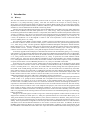
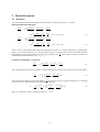
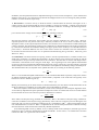
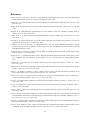
RegCM Version 4.0
User’s Guide
Nellie Elguindi, Xunqiang Bi, Filippo Giorgi, Badrinath Nagarajan,
Jeremy Pal, Fabien Solmon, Sara Rauscher, and Ashraf Zakey
Trieste, Italy
June 2010
1
Acknowledgements
This paper is dedicated to those that have contributed to the growth of RegCM system over the past 20+ years, the
members (800+) of the RegCNET, and the ICTP.
2
Abstract
As one of the main aims of the Abdus Salam International Centre for Theoretical Physics (ICTP) is to foster
the growth of advanced studies and research in developing countries, the main purpose of this Regional Climate
Model (REGional Climate Model (RegCM)) Tutorial Class Notes is to give model users a guide to learn the
whole RegCM Model System.
The RegCM Tutorial Class is offered as a part of extended hands-on lab sessions during a series of Workshops
organized by the Physics of Weather and Climate (PWC) group at the ICTP.
RegCM was originally developed at the National Center for Atmospheric Research (NCAR) and has been
mostly applied to studies of regional climate and seasonal predictability around the world. The workshop
participants are welcome to use RegCM for regional climate simulation over different areas of interest. The
RegCM is available on the World Wide Web at https://eforge.escience-lab.org/gf/project/regcm/wiki/.
3
Contents
1 Introduction
1.1 History . . . . . . . . . . . . . . . . . . . . . . . . . . . . . . . . . . . . . . . . . . . . . . . .
1.2 The RegCM Model Horizontal and Vertical Grid . . . . . . . . . . . . . . . . . . . . . . . . . .
1.3 Map Projections and Map-Scale Factors . . . . . . . . . . . . . . . . . . . . . . . . . . . . . . .
2 Model Description
2.1 Dynamics . . . . . . . . . . . . . . . . . . . . . . . . . .
2.2 Physics . . . . . . . . . . . . . . . . . . . . . . . . . . .
2.2.1 Radiation Scheme . . . . . . . . . . . . . . . . .
2.2.2 Land Surface Models . . . . . . . . . . . . . . . .
2.2.3 Planetary Boundary Layer Scheme . . . . . . . . .
2.2.4 Convective Precipitation Schemes . . . . . . . . .
2.2.5 Large-Scale Precipitation Scheme . . . . . . . . .
2.2.6 Ocean flux Parameterization . . . . . . . . . . . .
2.2.7 Prognostic Sea Surface Skin Temperature Scheme
2.2.8 Pressure Gradient Scheme . . . . . . . . . . . . .
2.2.9 Lake Model . . . . . . . . . . . . . . . . . . . . .
2.2.10 Aerosols and Dust (Chemistry Model) . . . . . . .
4
.
.
.
.
.
.
.
.
.
.
.
.
.
.
.
.
.
.
.
.
.
.
.
.
.
.
.
.
.
.
.
.
.
.
.
.
.
.
.
.
.
.
.
.
.
.
.
.
.
.
.
.
.
.
.
.
.
.
.
.
.
.
.
.
.
.
.
.
.
.
.
.
.
.
.
.
.
.
.
.
.
.
.
.
.
.
.
.
.
.
.
.
.
.
.
.
.
.
.
.
.
.
.
.
.
.
.
.
.
.
.
.
.
.
.
.
.
.
.
.
.
.
.
.
.
.
.
.
.
.
.
.
.
.
.
.
.
.
.
.
.
.
.
.
.
.
.
.
.
.
.
.
.
.
.
.
.
.
.
.
.
.
.
.
.
.
.
.
.
.
.
.
.
.
.
.
.
.
.
.
.
.
.
.
.
.
.
.
.
.
.
.
.
.
.
.
.
.
.
.
.
.
.
.
.
.
.
.
.
.
.
.
.
.
.
.
.
.
.
.
.
.
.
.
.
.
.
.
.
.
.
.
.
.
.
.
.
.
.
.
.
.
.
.
.
.
.
.
.
.
.
.
6
6
7
9
10
10
12
12
12
15
15
17
18
18
18
18
19
List of Figures
1
2
Schematic representation of the vertical structure of the model. This example is for 16 vertical
layers. Dashed lines denote half-sigma levels, solid lines denote full-sigma levels. (Adapted from
the PSU/NCAR Mesoscale Modeling System Tutorial Class Notes and User’s Guide.) . . . . . . .
Schematic representation showing the horizontal Arakawa B-grid staggering of the dot and cross
grid points. . . . . . . . . . . . . . . . . . . . . . . . . . . . . . . . . . . . . . . . . . . . . . .
7
8
List of Tables
1
2
3
Land Cover/Vegetation classes . . . . . . . . . . . . . . . . . . . . . . . . . . . . . . . . . . . .
BATS vegetation/land-cover . . . . . . . . . . . . . . . . . . . . . . . . . . . . . . . . . . . . .
Resolution for CLM input parameters . . . . . . . . . . . . . . . . . . . . . . . . . . . . . . . .
5
13
14
15
1 Introduction
1.1
History
The idea that limited area models (LAMs) could be used for regional studies was originally proposed by
Dickinson et al. [1989] and Giorgi [1990]. This idea was based on the concept of one-way nesting, in
which large scale meteorological fields from General Circulation Model (GCM) runs provide initial and timedependent meteorological lateral boundary conditions (LBCs) for high resolution Regional Climate Model (RCM)
simulations, with no feedback from the RCM to the driving GCM.
The first generation NCAR RegCM was built upon the NCAR-Pennsylvania State University (PSU) Mesoscale
Model version 4 (MM4) in the late 1980s [Dickinson et al., 1989; Giorgi, 1989]. The dynamical component of
the model originated from the MM4, which is a compressible, finite difference model with hydrostatic balance and
vertical σ-coordinates. Later, the use of a split-explicit time integration scheme was added along with an algorithm
for reducing horizontal diffusion in the presence of steep topographical gradients [Giorgi et al., 1993a, b]. As
a result, the dynamical core of the RegCM is similar to that of the hydrostatic version of Mesoscale Model
version 5 (MM5) [Grell et al., 1994].
For application of the MM4 to climate studies, a number of physics parameterizations were replaced, mostly
in the areas of radiative transfer and land surface physics, which led to the first generation RegCM [Dickinson
et al., 1989; Giorgi, 1990]. The first generation RegCM included the Biosphere-Atmosphere Transfer Scheme,
BATS, [Dickinson et al., 1986] for surface process representation, the radiative transfer scheme of the Community
Climate Model version 1 (CCM1), a medium resolution local planetary boundary layer scheme, the Kuo-type
cumulus convection scheme of [Anthes, 1977] and the explicit moisture scheme of [Hsie et al., 1984].
A first major upgrade of the model physics and numerical schemes was documented by [Giorgi et al., 1993a, b],
and resulted in a second generation RegCM, hereafter referred to as REGional Climate Model version 2 (RegCM2).
The physics of RegCM2 was based on that of the NCAR Community Climate Model version 2 (CCM2) [Hack
et al., 1993], and the mesoscale model MM5 [Grell et al., 1994]. In particular, the CCM2 radiative transfer
package [Briegleb, 1992] was used for radiation calculations, the non local boundary layer scheme of [Holtslag
et al., 1990] replaced the older local scheme, the mass flux cumulus cloud scheme of [Grell, 1993] was added as
an option, and the latest version of BATS1E [Dickinson et al., 1993] was included in the model.
In the last few years, some new physics schemes have become available for use in the RegCM, mostly based
on physics schemes of the latest version of the Community Climate Model (CCM), Community Climate Model
version 3 (CCM3) [Kiehl et al., 1996]. First, the CCM2 radiative transfer package has been replaced by that of
the CCM3. In the CCM2 package, the effects of H2 O, O3 , O2 , CO2 and clouds were accounted for by the model.
Solar radiative transfer was treated with a δ-Eddington approach and cloud radiation depended on three cloud
parameters, the cloud fractional cover, the cloud liquid water content, and the cloud effective droplet radius. The
CCM3 scheme retains the same structure as that of the CCM2, but it includes new features such as the effect of
additional greenhouse gases (NO2 , CH4 , CFCs), atmospheric aerosols, and cloud ice.
The other primary changes are in the areas of cloud and precipitation processes. The original explicit moisture
scheme of Hsie et al. [1984] has been substituted with a simplified version because the original scheme was
computationally too expensive to be run in climate mode. In the simplified scheme only a prognostic equation
for cloud water is included, which accounts for cloud water formation, advection and mixing by turbulence, reevaporation in sub-saturated conditions, and conversion into rain via a bulk autoconversion term. The main novelty
of this scheme does not reside of course in the simplistic microphysics, but in the fact that the prognosed cloud
water variable is directly used in the cloud radiation calculations. In the previous versions of the model, cloud
water variables for radiation calculations were diagnosed in terms of the local relative humidity. This new feature
adds a very important and far reaching element of interaction between the simulated hydrologic cycle and energy
budget calculations.
Changes in the model physics include a large-scale cloud and precipitation scheme which accounts for the
subgrid-scale variability of clouds [Pal et al., 2000], new parameterizations for ocean surface fluxes [Zeng et al.,
1998], and a cumulus convection scheme [Emanuel, 1991; Emanuel and Zivkovic-Rothman, 1999]. Also new in the
model is a mosaic-type parameterization of subgrid-scale heterogeneity in topography and land use [Giorgi et al.,
2003b]. Other improvements in RegCM3 involve the input data. The USGS Global Land Cover Characterization
and Global 30 Arc-Second Elevation datasets are now used to create the terrain files. In addition, NCEP and
ECMWF global reanalysis datasets are used for the intial and boundary conditions. Lastly, improvements in the
user-friendliness of the model have been made. New scripts have been included which make running the programs
6
Figure 1: Schematic representation of the vertical structure of the model. This example is for 16 vertical layers.
Dashed lines denote half-sigma levels, solid lines denote full-sigma levels. (Adapted from the PSU/NCAR
Mesoscale Modeling System Tutorial Class Notes and User’s Guide.)
easier. Also, a new website has been developed where users can freely download the entire RegCM system, as well
as all of the input data necessary for a simulation.
The RegCM modeling system has four components: Terrain, ICBC, RegCM, and Postprocessor. Terrain
and ICBC are the two components of RegCM preprocessor. Terrestrial variables (including elevation, landuse
and sea surface temperature) and three-dimensional isobaric meteorological data are horizontally interpolated
from a latitude-longitude mesh to a high-resolution domain on either a Rotated (and Normal) Mercator, Lambert
Conformal, or Polar Stereographic projection. Vertical interpolation from pressure levels to the σ coordinate
system of RegCM is also performed. σ surfaces near the ground closely follow the terrain, and the higher-level σ
surfaces tend to approximate isobaric surfaces.
Since the vertical and horizontal resolution and domain size can vary, the modeling package programs employ
parameterized dimensions requiring a variable amount of core memory, and the requisite hard-disk storage amount
is varied accordingly.
7
Figure 2: Schematic representation showing the horizontal Arakawa B-grid staggering of the dot and cross grid
points.
1.2
The RegCM Model Horizontal and Vertical Grid
It is useful to first introduce the model’s grid configuration. The modeling system usually gets and analyzes its data
on pressure surfaces, but these have to be interpolated to the model’s vertical coordinate before input to the model.
The vertical coordinate is terrain-following (Figure 1) meaning that the lower grid levels follow the terrain while
the upper surface is flatter. Intermediate levels progressively flatten as the pressure decreases toward the top of the
model. A dimensionless σ coordinate is used to define the model levels where p is the pressure, pt is a specified
constant top pressure, ps is the surface pressure.
σ=
(p − pt )
(ps − pt )
(1)
It can be seen from the equation and Figure 1 that σ is zero at the top and one at the surface, and each model
level is defined by a value of σ. The model vertical resolution is defined by a list of values between zero and one
that do not necessarily have to be evenly spaced. Commonly the resolution in the boundary layer is much finer
than above, and the number of levels may vary upon the user demand.
The horizontal grid has an Arakawa-Lamb B-staggering of the velocity variables with respect to the scalar
variables. This is shown in Figure 2 where it can be seen that the scalars (T, q, p, etc) are defined at the center of
the grid box, while the eastward (u) and northward (v) velocity components are collocated at the corners. The center
points of grid squares will be referred to as cross points, and the corner points are dot points. Hence horizontal
velocity is defined at dot points. Data is input to the model, the preprocessors do the necessary interpolation to
assure consistency with the grid.
8
All the above variables are defined in the middle of each model vertical layer, referred to as half-levels and
represented by the dashed lines in Figure 1. Vertical velocity is carried at the full levels (solid lines). In defining
the sigma levels it is the full levels that are listed, including levels at σ = 0 and 1. The number of model layers is
therefore always one less than the number of full sigma levels.
The finite differencing in the model is, of course, crucially dependent upon the grid staggering wherever
gradients or averaging are represented terms in the equation.
1.3
Map Projections and Map-Scale Factors
The modeling system has a choice of four map projections. Lambert Conformal is suitable for mid-latitudes, Polar
Stereographic for high latitudes, Normal Mercator for low latitudes, and Rotated Mercator for extra choice. The
x and y directions in the model do not correspond to west-east and north-south except for the Normal Mercator
projection, and therefore the observed wind generally has to be rotated to the model grid, and the model u and v
components need to be rotated before comparison with observations. These transformations are accounted for in
the model pre-processors that provide data on the model grid (Please note that model output of u and v components,
raw or postprocessed, should be rotated to a lat/lon grid before comparing to observations). The map scale factor,
m, is defined by
m = (distance on grid) / (actual distance on earth)
and its value is usually close to one, varying with latitude. The projections in the model preserve the shape of
small areas, so that dx=dy everywhere, but the grid length varies across the domain to allow a representation of a
spherical surface on a plane surface. Map-scale factors need to be accounted for in the model equations wherever
horizontal gradients are used.
9
2 Model Description
2.1
Dynamics
The model dynamic equations and numerical discretization are described by Grell et al. [1994].
Horizontal Momentum Equations
∗
∂p∗ u
∂p∗ uσ˙
∂p uu/m ∂p∗ vu/m
−
= −m2
+
∂t
∂x
∂y
∂σ
RTv
∂p∗ ∂φ
∗
−mp
+ f p∗ v + FH u + FV u,
+
(p∗ + pt /σ) ∂x
∂x
∗
∂p∗ vσ˙
∂p∗ vv/m
∂p∗ v
2 ∂p uv/m
−
= −m
+
∂t
∂x
∂y
∂σ
RTv
∂p∗ ∂φ
−mp∗
+ f p∗ u + FH v + FV v,
+
(p∗ + pt /σ) ∂y
∂y
(2)
(3)
where u and v are the eastward and northward components of velocity, Tv is virtual temperature, φ is geopotential
height, f is the coriolis parameter, R is the gas constant for dry air, m is the map scale factor for either the Polar
Stereographic, Lambert Conformal, or Mercator map projections, σ˙ = dσ
dt , and FH and FV represent the effects of
horizontal and vertical diffusion, and p∗ = ps − pt .
˙ Equations
Continuity and Sigmadot (σ)
∂p∗
= −m2
∂t
∂p∗ σ˙
∂p∗ u/m ∂p∗ v/m
−
+
.
∂x
∂y
∂σ
(4)
The vertical integral of Equation 4 is used to compute the temporal variation of the surface pressure in the model,
∂p∗
= −m2
∂t
Z 1 ∗
∂p u/m
∂x
0
+
∂p∗ v/m
dσ.
∂y
(5)
˙
After calculation of the surface-pressure tendency ∂p
∂t , the vertical velocity in sigma coordinates (σ) is computed
at each level in the model from the vertical integral of Equation 4.
∗
Z ∂p u/m ∂p∗ v/m
1 σ ∂p∗
2
dσ′,
(6)
+m
+
σ˙ = − ∗
p 0
∂t
∂x
∂y
∗
˙ = 0) = 0.
where σ′ is a dummy variable of integration and σ(σ
10
Thermodynamic Equation and Equation for Omega (ω)
The thermodynamic equation is
∗
∂p∗ T σ˙
∂p∗ vT /m
∂p∗ T
2 ∂p uT /m
−
= −m
+
+
∂t
∂x
∂y
∂σ
RTv ω
p∗ Q
+
+ FH T + FV T,
c pm (σ + Pt /past ) c pm
(7)
where c pm is the specific heat for moist air at constant pressure, Q is the diabatic heating, FH T represents the effect
of horizontal diffusion, FV T represents the effect of vertical mixing and dry convective adjustment, and ω is
ω = p∗ σ˙ + σ
d p∗
,
dt
(8)
where,
∂p∗
∂p∗
∂p∗
d p∗
.
=
+m u
+v
dt
∂t
∂x
∂y
(9)
The expression for c pm = c p (1 + 0.8qv ),
where c p is the specific heat at constant pressure for dry air and qv is the mixing ratio of water vapor.
Hydrostatic Equation
The hydrostatic equation is used to compute the geopotential heights from the virtual temperature Tv ,
∂φ
qc + qr −1
= −RTv 1 +
,
∂ln(σ + pt /p∗ )
1 + qv
(10)
where Tv = T (1 + 0.608qv ), qv , qc , and qr are the water vapor, cloud water or ice, and rain water or snow, mixing
ratios.
11
2.2
Physics
2.2.1
Radiation Scheme
RegCM4 uses the radiation scheme of the NCAR CCM3, which is described in Kiehl et al. [1996]. Briefly, the
solar component, which accounts for the effect of O3 , H2 O, CO2 , and O2 , follows the δ-Eddington approximation
of Kiehl et al. [1996]. It includes 18 spectral intervals from 0.2 to 5 µm. The cloud scattering and absorption
parameterization follow that of Slingo [1989], whereby the optical properties of the cloud droplets (extinction
optical depth, single scattering albedo, and asymmetry parameter) are expressed in terms of the cloud liquid water
content and an effective droplet radius. When cumulus clouds are formed, the gridpoint fractional cloud cover is
such that the total cover for the column extending from the model-computed cloud-base level to the cloud-top level
(calculated assuming random overlap) is a function of horizontal gridpoint spacing. The thickness of the cloud
layer is assumed to be equal to that of the model layer, and a different cloud water content is specified for middle
and low clouds.
2.2.2
Land Surface Models
BATS (default): BATS is a surface package designed to describe the role of vegetation and interactive soil moisture
in modifying the surface-atmosphere exchanges of momentum, energy, and water vapor (see Dickinson et al. [1993]
for details). The model has a vegetation layer, a snow layer, a surface soil layer, 10 cm thick, or root zone layer,
1-2 m thick, and a third deep soil layer 3 m thick. Prognostic equations are solved for the soil layer temperatures
using a generalization of the force-restore method of Deardoff [1978]. The temperature of the canopy and canopy
foilage is calculated diagnostically via an energy balance formulation including sensible, radiative, and latent heat
fluxes.
The soil hydrology calculations include predictive equations for the water content of the soil layers. These
equations account for precipitation, snowmelt, canopy foiliage drip, evapotranspiration, surface runoff, infiltration
below the root zone, and diffusive exchange of water between soil layers. The soil water movement formulation is
obtained from a fit to results from a high-resolution soil model Dic [1984] and the surface runoff rates are expressed
as functions of the precipitation rates and the degree of soil water saturation. Snow depth is prognostically
calculated from snowfall, snowmelt, and sublimation. Precipitation is assumed to fall in the form of snow if
the temperature of the lowest model level is below 271 K.
Sensible heat, water vapor, and momentum fluxes at the surface are calculated using a standard surface drag
coefficient formulation based on surface-layer similarity theory. The drag coefficient depends on the surface
roughness length and on the atmospheric stability in the surface layer. The surface evapotranspiration rates depend
on the availability of soil water. Biosphere-Atmosphere Transfer Scheme (BATS) has 20 vegetation types (Table 2;
soil textures ranging from coarse (sand), to intermediate (loam), to fine (clay); and different soil colors (light to
dark) for the soil albedo calculations. These are described in Dickinson et al. [1986].
In the latest release version, additional modifications have been made to BATSin order to account for
the subgrid variability of topography and landcover using a mosaic-type approach [Giorgi et al., 2003a].
Thismodification adopts a regular fine-scale surface subgrid for eachcoarse model grid cell. Meteorological
variables are disaggregatedfrom the coarse grid to the fine grid based on the elevationdifferences. The BATS
calculations are then performed separatelyfor each subgrid cell, and surface fluxes are reaggregated onto thecoarse
grid cell for input to the atmospheric model. Thisparameterization showed a marked improvement in the
representation ofthe surface hydrological cycle in mountainous regions [Giorgi et al., 2003a].
CLM (optional): The Community Land Model (CLM; Oleson et al. [2008]) is the land surface model developed
by the National Center of Atmospheric Research (NCAR) as part of the Community Climate System Model
(CCSM), described in detail in Collins et al. [2006]. CLM version 3.5 was coupled to RegCM for a more detailed
land surface description option. CLM contains five possible snow layers with an additional representation of trace
snow and ten unevenly spaced soil layers with explicit solutions of temperature, liquid water and ice water in each
layer. To account for land surface complexity within a climate model grid cell, CLM uses a tile or mosaic approach
to capture surface heterogeneity. Each CLM gridcell contains up to four different land cover types (glacier, wetland,
lake, and vegetated), where the vegetated fraction can be further divided into 17 different plant functional types.
Hydrological and energy balance equations are solved for each land cover type and aggregated back to the gridcell
level. A detailed discussion of CLM version 3 implemented in RegCM3 and comparative analysis of land surface
parameterization options is presented in Steiner et al. [2009]. Since CLM was developed for the global scale,
12
Table 1:
1.
2.
3.
4.
5.
6.
7.
8.
9.
10.
11.
12.
13.
14.
15.
16.
17.
18.
19.
20.
Land Cover/Vegetation classes
Crop/mixed farming
Short grass
Evergreen needleleaf tree
Deciduous needleleaf tree
Deciduous broadleaf tree
Evergreen broadleaf tree
Tall grass
Desert
Tundra
Irrigated Crop
Semi-desert
Ice cap/glacier
Bog or marsh
Inland water
Ocean
Evergreen shrub
Deciduous shrub
Mixed Woodland
Forest/Field mosaic
Water and Land mixture
several input files and processes were modified to make it more appropriate for regional simulations, including
(1) the use of high resolution input data, (2) soil moisture initialization, and (3) and an improved treatment of grid
cells along coastlines. For the model input data, CLM requires several time-invariant surface input parameters: soil
color, soil texture, percent cover of each land surface type, leaf and stem area indices, maximum saturation fraction,
and land fraction [Lawrence and Chase, 2007]. Table 3 shows the resolution for each input parameter used at the
regional scale in RegCM-CLM compared to resolutions typically used for global simulations. The resolution of
surface input parameters was increased for several parameters to capture surface heterogeneity when interpolating
to the regional climate grid. Similar to Lawrence and Chase [2007], the number of soil colors was extended from 8
to 20 classes to resolve regional variations. The second modification was to update the soil moisture initialization
based on a climatological soil moisture average [Giorgi and Bates, 1989] over the use of constant soil moisture
content throughout the grid generally used for global CLM. By using a climatological average for soil moisture,
model spin-up time is reduced with regards to deeper soil layers. The third modification to the CLM is the inclusion
of a mosaic approach for gridcells that contain both land and ocean surface types. With this approach, a weighted
average of necessary surface variables was calculated for land/ocean gridcells using the land fraction input dataset.
This method provides a better representation of coastlines using the high-resolution land fraction data described in
Table 3. For a more detailed description of CLM physics parameterizations see Oleson [2004].
13
Parameter
14
Max fractional
vegetation cover
Difference between max
fractional vegetation
cover and cover at 269 K
Roughness length (m)
Displacement height (m)
Min stomatal
resistence (s/m)
Max Leaf Area Index
Min Leaf Area Index
Stem (dead matter
area index)
Inverse square root of
leaf dimension (m−1/2 )
Light sensitivity
factor (m2 W−1 )
Upper soil layer
depth (mm)
Root zone soil
layer depth (mm)
Depth of total
soil (mm)
Soil texture type
Soil color type
Vegetation albedo for
wavelengths < 0.7 µ m
Vegetation albedo for
wavelengths > 0.7 µ m
Table 2: BATS vegetation/land-cover
Land Cover/Vegetation Type
6
7
8
9
10
11
12
1
2
3
4
5
13
14
15
16
17
18
19
20
0.85
0.80
0.80
0.80
0.80
0.90
0.80
0.00
0.60
0.80
0.35
0.00
0.80
0.00
0.00
0.80
0.80
0.80
0.80
0.80
0.6
0.08
0.0
0.1
0.05
0.0
0.1
1.00
9.0
0.3
1.00
9.0
0.5
0.80
0.0
0.3
2.00
18.0
0.0
0.10
0.0
0.2
0.05
0.0
0.6
0.04
0.0
0.1
0.06
0.0
0.0
0.10
0.0
0.4
0.01
0.0
0.0
0.03
0.0
0.0
0.0004
0.0
0.2
0.0004
0.0
0.3
0.10
0.0
0.2
0.10
0.0
0.4
0.80
0.0
0.4
0.3
0.0
0.3
0.0
45
6
0.5
60
2
0.5
80
6
5
80
6
1
120
6
1
60
6
5
60
6
0.5
200
0
0
80
6
0.5
45
6
0.5
150
6
0.5
200
0
0
45
6
0.5
200
0
0
200
0
0
80
6
5
120
6
1
100
6
3
120
6
0.5
120
6
0.5
0.5
4.0
2.0
2.0
2.0
2.0
2.0
0.5
0.5
2.0
2.0
2.0
2.0
2.0
2.0
2.0
2.0
2.0
2.0
2.0
10
5
5
5
5
5
5
5
5
5
5
5
5
5
5
5
5
5
5
5
0.02
0.02
0.06
0.06
0.06
0.06
0.02
0.02
0.02
0.02
0.02
0.02
0.02
0.02
0.02
0.02
0.02
0.06
0.02
0.02
100
100
100
100
100
100
100
100
100
100
100
100
100
100
100
100
100
100
100
100
1000
1000
1500
1500
2000
1500
1000
1000
1000
1000
1000
1000
1000
1000
1000
1000
1000
2000
2000
2000
3000
6
5
3000
6
3
3000
6
4
3000
6
4
3000
7
4
3000
8
4
3000
6
4
3000
3
1
3000
6
3
3000
6
3
3000
5
2
3000
12
1
3000
6
5
3000
6
5
3000
6
5
3000
6
4
3000
5
3
3000
6
4
3000
6
4
3000
0
0
0.10
0.10
0.05
0.05
0.08
0.04
0.08
0.20
0.10
0.08
0.17
0.80
0.06
0.07
0.07
0.05
0.08
0.06
0.06
0.06
0.30
0.30
0.23
0.23
0.28
0.20
0.30
0.40
0.30
0.28
0.34
0.60
0.18
0.20
0.20
0.23
0.28
0.24
0.18
0.18
Table 3: Resolution for CLM input parameters
Input data
Grid Spacing Lon range Lat range
Glacier
0.05◦ x 0.05◦ ±179.975 ±89.975
Lake
0.05◦ x 0.05◦ ±179.975 ±89.975
Wetland
0.05◦ x 0.05◦ ±179.975 ±89.975
Land fraction
0.05◦ x 0.05◦ ±179.975 ±89.975
LAI/SAI
0.5◦ x 0.5◦
±179.75
±89.75
PFT
0.5◦ x 0.5◦
±179.75
±89.75
Soil color
0.05◦ x 0.05◦ ±179.975 ±89.975
Soil texture
0.05◦ x 0.05◦ ±179.975 ±89.975
Max. sat. area
0.5◦ x 0.5◦
±179.75
±89.75
2.2.3
Planetary Boundary Layer Scheme
The planetary boundary layer scheme, developed by Holtslag et al. [1990], is based on a nonlocal diffusion
concept that takes into account countergradient fluxes resulting from large-scale eddies in an unstable, well-mixed
atmosphere. The vertical eddy flux within the PBL is given by
Fc = −Kc
∂C
− γc
∂z
(11)
where γc is a “countergradient” transport term describing nonlocal transport due to dry deep convection. The eddy
diffusivity is given by the nonlocal formulation
z2
,
Kc = kwt z 1 −
h
(12)
where k is the von Karman constant; wt is a turbulent convective velocity that depends on the friction velocity,
height, and the Monin–Obhukov length; and h is the PBL height. The countergradient term for temperature and
water vapor is given by
γc = C
φc 0
,
wt h
(13)
where C is a constant equal to 8.5, and φc 0 is the surface temperature or water vapor flux. Equation 13 is applied
between the top of the PBL and the top of the surface layer, which is assumed to be equal to 0.1h. Outside this
region and for momentum, γc is assumed to be equal to 0.
For the calculation of the eddy diffusivity and countergradient terms, the PBL height is diagnostically computed
from
h=
Ric r[u(h)2 + v(h)2 ]
(g/θs )[θv (h) − θs ]
(14)
where u(h), v(h), and θv are the wind components and the virtual potential temperature at the PBL height, g is
gravity, Ric r is the critical bulk Richardson number, and θs is an appropriate temperature of are near the surface.
Refer to Holtslag et al. [1990] and Holtslag and Boville [1993] for a more detailed description.
2.2.4
Convective Precipitation Schemes
Convective precipitation is computed using one of three schemes: (1) Modified-Kuo scheme Anthes [1977]; (2)
Grell scheme Grell [1993]; and (3) MIT-Emanuel scheme [Emanuel, 1991; Emanuel and Zivkovic-Rothman, 1999].
15
In addition, the Grell parameterization is implemented using one of two closure assumptions: (1) the Arakawa and
Schubert closure Grell et al. [1994] and (2) the Fritsch and Chappell closure Fritsch and Chappell [1980], hereafter
refered to as AS74 and FC80, respectively.
1. Kuo Scheme: Convective activity in the Kuo scheme is initiated when the moisture convergence M in a
column exceeds a given threshold and the vertical sounding is convectively unstable. A fraction of the moisture
convergence β moistens the column and the rest is converted into rainfall PCU according to the following relation:
PCU
= M(1 − β).
β is a function of the average relative humidity RH of the sounding as follows:
RH ≥ 0.5
2(1 − RH)
β =
1.0
otherwise
(15)
(16)
Note that the moisture convergence term includes only the advective tendencies for water vapor. However,
evapotranspiration from the previous time step is indirectly included in M since it tends to moisten the lower
atmosphere. Hence, as the evapotranspiration increases, more and more of it is converted into rainfall assuming the
column is unstable. The latent heating resulting from condensation is distributed between the cloud top and bottom
by a function that allocates the maximum heating to the upper portion of the cloud layer. To eliminate numerical
point storms, a horizontal diffusion term and a time release constant are included so that the redistributions
of moisture and the latent heat release are not performed instantaneously [Giorgi and Bates, 1989; Giorgi and
Marinucci, 1991].
2. Grell Scheme: The Grell scheme Grell [1993], similar to the AS74 parameterization, considers clouds as two
steady-state circulations: an updraft and a downdraft. No direct mixing occurs between the cloudy air and the
environmental air except at the top and bottom of the circulations. The mass flux is constant with height and no
entrainment or detrainment occurs along the cloud edges. The originating levels of the updraft and downdraft
are given by the levels of maximum and minimum moist static energy, respectively. The Grell scheme is activated
when a lifted parcel attains moist convection. Condensation in the updraft is calculated by lifting a saturated parcel.
The downdraft mass flux (m0 ) depends on the updraft mass flux (mb ) according to the following relation:
m0 =
βI1
mb ,
I2
(17)
where I1 is the normalized updraft condensation, I2 is the normalized downdraft evaporation, and β is the fraction
of updraft condensation that re-evaporates in the downdraft. β depends on the wind shear and typically varies
between 0.3 and 0.5. Rainfall is given by
PCU
=
I1 mb (1 − β).
(18)
Heating and moistening in the Grell scheme are determined both by the mass fluxes and the detrainment at the
cloud top and bottom. In addition, the cooling effect of moist downdrafts is included.
Due to the simplistic nature of the Grell scheme, several closure assumptions can be adopted. RegCM4’s earlier
version directly implements the quasi-equilibrium assumption of AS74. It assumes that convective clouds stabilize
the environment as fast as non-convective processes destabilize it as follows:
mb =
ABE ′′ − ABE
,
NA∆t
(19)
where ABE is the buoyant energy available for convection, ABE ′′ is the amount of buoyant energy available for
convection in addition to the buoyant energy generated by some of the non-convective processes during the time
interval ∆t, and NA is the rate of change of ABE per unit mb . The difference ABE ′′ − ABE can be thought of as the
rate of destabilization over time ∆t. ABE ′′ is computed from the current fields plus the future tendencies resulting
from the advection of heat and moisture and the dry adiabatic adjustment.
In the latest RegCM4 version, by default, we use a stability based closure assumption, the FC80 type closure
assumption, that is commonly implemented in GCMs and RCMs. In this closure, it is assumed that convection
removes the ABE over a given time scale as follows:
mb =
ABE
,
NAτ
16
(20)
where τ is the ABE removal time scale.
The fundamental difference between the two assumptions is that the AS74 closure assumption relates the
convective fluxes and rainfall to the tendencies in the state of the atmosphere, while the FC80 closure assumption
relates the convective fluxes to the degree of instability in the atmosphere. Both schemes achieve a statistical
equilibrium between convection and the large-scale processes.
3. MIT-Emanuel scheme: The newest cumulus convection option to the REGional Climate Model version 4
(RegCM4) is theMassachusetts Institute of Technology (MIT) scheme. More detailed descriptions can be found
in Emanuel [1991] andEmanuel and Zivkovic-Rothman [1999]. The scheme assumes that the mixing in clouds
ishighly episodic and inhomogeneous (as opposed to a continuousentraining plume) and considers convective
fluxes based on anidealized model of sub-cloud-scale updrafts and downdrafts.Convection is triggered when the
level of neutral buoyancy is greaterthan the cloud base level. Between these two levels, air is liftedand a fraction of
the condensed moisture forms precipitation while theremaining fraction forms the cloud. The cloud is assumed to
mix withthe air from the environment according to a uniform spectrum ofmixtures that ascend or descend to their
respective levels of neutralbuoyancy. The mixing entrainment and detrainment rates are functionsof the vertical
gradients of buoyancy in clouds. The fraction of thetotal cloud base mass flux that mixes with its environment at
eachlevel is proportional to the undiluted buoyancy rate of change withaltitude. The cloud base upward mass flux
is relaxed towards thesub-cloud layer quasi equilibrium.
In addition to a more physical representation of convection, theMIT-Emanuel scheme offers several advantages
compared to theother RegCM4 convection options. For instance, it includes aformulation of the auto-conversion
of cloud water into precipitationinside cumulus clouds, and ice processes are accounted for by allowingthe autoconversion threshold water content to be temperaturedependent. Additionally, the precipitation is added to a
single,hydrostatic, unsaturated downdraft that transports heat and water.Lastly, the MIT-Emanuel scheme considers
the transport of passive tracers.
2.2.5
Large-Scale Precipitation Scheme
Subgrid Explicit Moisture Scheme (SUBEX) is used to handle nonconvective clouds and precipitation resolved
by the model. This is one of the new components of the model. SUBEX accounts for the subgrid variability in
clouds by linking the average grid cell relative humidity to the cloud fraction and cloud water following the work
of Sundqvist et al. [1989].
The fraction of the grid cell covered by clouds, FC, is determined by,
r
RH − RHmin
(21)
FC =
RHmax − RHmin
where RHmin is the relative humidity threshold at which clouds begin to form, and RHmax is the relative humidity
where FC reaches unity. FC is assumed to be zero when RH is less than RHmin and unity when RH is greater than
RHmax .
Precipitation P forms when the cloud water content exceeds the autoconversion threshold Qth c according to the
following relation:
P = Cppt (Qc /FC − Qc th )FC
(22)
where 1/Cppt can be considered the characteristic time for which cloud droplets are converted to raindrops. The
threshold is obtained by scaling the median cloud liquid water content equation according to the following:
Qth c = Cacs 10−0.49+0.013T ,
(23)
where T is temperature in degrees Celsius, and Cacs is the autoconversion scale factor. Precipitation is assumed to
fall instantaneously.
SUBEX also includes simple formulations for raindrop accretion and evaporation. The formulation for the
accretion of cloud droplets by falling rain droplets is based on the work of Beheng [1994] and is as follows:
Pacc = Cacc QPsum
(24)
where Pacc is the amount of accreted cloud water, Cacc is the accretion rate coefficient, and Psum is the accumulated
precipitation from above falling through the cloud.
17
Precipitation evaporation is based on the work of Sundqvist et al. [1989] and is as follows,
Pevap = Cevap (1 − RH)P1/2 sum
(25)
where Pevap is the amount of evaporated precipitation, and Cevap is the rate coefficient. For a more detailed
description of SUBEX and a list of the parameter values refer to Pal et al. [2000].
2.2.6
Ocean flux Parameterization
1. BATS: BATS uses standard Monin-Obukhov similarity relations to compute the fluxes with no special treatment
of convective and very stable conditions. In addition, the roughness length is set to a constant, i.e. it is not a
function of wind and stability.
2. Zeng: The Zeng scheme describes all stability conditions and includes a gustiness velocity to account for the
additional flux induced by boundary layer scale variability. Sensible heat (SH), latent heat (LH), and momentum
(τ) fluxes between the sea surface and lower atmosphere are calculated using the following bulk aerodynamic
algorithms,
τ = ρa u∗ 2 (ux 2 + uy 2 )1/2 /u
(26)
SH = −ρaCpa u∗ θ∗
(27)
LH = −ρa Le u∗ q∗
(28)
where ux and uy are mean wind components, u∗ is the frictional wind velocity, θ∗ is the temperature scaling
parameter, q∗ is the specific humidity scaling parameter, ρa is air density, Cpa is specific heat of air, and Le is the
latent heat of vaporization. For further details on the calculation of these parameters refer to Zeng et al. [1998].
2.2.7
Prognostic Sea Surface Skin Temperature Scheme
RegCM4 contains a option which allows for the computation of sea surface skin temperature as a prognostic
variable following the scheme of Zeng [2005]. This allows for a realistic representation of the diurnal sea surface
skin temperature, leading to improvements in the surface fluxes thus air-sea interactions. The scheme is based on
a two-layer model which includes warm layer/cool skin effects as described by Fairall et al.). Temperatures in the
two layers are calculated using a one-dimensional heat transfer equation and boundary conditions determined by
surface to atmosphere fluxes (latent, sensible and radiative) and a 3 m depth sea surface temperature taken from
the prescribed SSTs.
2.2.8
Pressure Gradient Scheme
Two options are available for calculating the pressure gradient force. The normal way uses the full fields. The
other way is the hydrostatic deduction scheme which makes use of a perturbation temperature. In this scheme,
extra smoothing on the top is done in order to reduce errors related to the PGF calculation.
2.2.9
Lake Model
The lake model developed by Hostetler et al. [1993] can be interactively coupled to the atmospheric model. In the
lake model, fluxes of heat, moisture, and momentum are calculated based on meteorological inputs and the lake
surface temperature and albedo. Heat is transferred vertically between lake model layers by eddy and convective
mixing. Ice and snow may cover part or all of the lake surface.
In the lake model, the prognostic equation for temperature is,
∂2 T
∂T
= (ke + km ) 2
∂t
∂z
(29)
where T is the temperature of the lake layer, and ke and km are the eddy and molecular diffusivities, respectively.
The parameterization of Henderson-Sellers [1986] is used to calculate ke and km is set to a constant value of
39 × 10−7 m2 s−1 except under ice and at the deepest points in the lake.
18
Sensible and latent heat fluxes from the lake are calculated using the BATS parameterizations Dickinson et al.
[1993]. The bulk aerodynamic formulations for latent heat flux (Fq ) and sensible heat flux (Fs ) are as follows,
Fq = ρaCDVa (qs − qa )
(30)
Fs = ρaCpCDVa (Ts − Ta )
(31)
where the subscripts s and a refer to surface and air, respectively; ρa is the density of air, Va is the wind speed, Cp ,
q is specific humidity, and T is temperature. The momentum drag coefficient, CD , depends on roughness length
and the surface bulk Richardson number.
Under ice-free conditions, the lake surface albedo is calculated as a function of solar zenith angle HendersonSellers [1986]. Longwave radiation emitted from the lake is calculated according to the Stefan-Boltzmann law. The
lake model uses the partial ice cover scheme of Patterson and Hamblin [1988] to represent the different heat and
moisture exchanges between open water and ice surfaces and the atmosphere, and to calculate the surface energy
of lake ice and overlying snow. For further details refer to Hostetler et al. [1993] and Small and Sloan [1999].
2.2.10
Aerosols and Dust (Chemistry Model)
The representation of dust emission processes is a key element in a dust model and depends on the wind conditions,
the soil characteristics and the particle size. Following Marticorena and Bergametti (1995) and Alfaro and
Gomes (2001), here the dust emission calculation is based on parameterizations of soil aggregate saltation and
sandblasting processes. The main steps in this calculation are: The specification of soil aggregate size distribution
for each model grid cell, the calculation of a threshold friction velocity leading to erosion and saltation processes,
the calculation of the horizontal saltating soil aggregate mass flux, and finally the calculation of the vertical
transportable dust particle mass flux generated by the saltating aggregates. In relation to the BATS interface,
these parameterizations become effective in the model for cells dominated by desert and semi desert land cover.
19
References
Climate Processes and Climate Sensitivity, chap. Modeling evapotranspiration processes for three-dimensional
global climate models, pp. 52–72, American Geophysical Union, 1984.
Anthes, R. A., A cumulus parameterization scheme utilizing a one-dimensional cloud model, Mon. Wea. Rev., 105,
270–286, 1977.
Beheng, K. D., A parameterization of warm cloud microphysical conversion processes, Atmos. Res., 33, 193–206,
1994.
Briegleb, B. P., Delta-eddington approximation for solar radiation in the ncar community climate model, J.
Geophys. Res., 97, 7603–7612, 1992.
Collins, W. D., et al., The Community Climate System Model version 3 (CCSM3), Journal of Climate, 19, 2122–
2143, 2006.
Deardoff, J. W., Efficient prediction of ground surface temperature and moisture with inclusion of a layer of
vegetation, J. Geophys. Res., 83, 1889–1903, 1978.
Dickinson, R. E., P. J. Kennedy, A. Henderson-Sellers, and M. Wilson, Biosphere-atmosphere transfer
scheme (bats) for the ncar community climate model, Tech. Rep. NCARE/TN-275+STR, National Center for
Atmospheric Research, 1986.
Dickinson, R. E., R. M. Errico, F. Giorgi, and G. T. Bates, A regional climate model for the western United States,
Climatic Change, 15, 383–422, 1989.
Dickinson, R. E., A. Henderson-Sellers, and P. J. Kennedy, Biosphere-atmosphere transfer scheme (bats) version
1e as coupled to the ncar community climate model, Tech. rep., National Center for Atmospheric Research,
1993.
Emanuel, K. A., A scheme for representing cumulus convection in large-scale models, J. Atmos. Sci., 48(21),
2313–2335, 1991.
Emanuel, K. A., and M. Zivkovic-Rothman, Development and evaluation of a convection scheme for use in climate
models, J. Atmos. Sci., 56, 1766–1782, 1999.
Fairall, C., E. Bradley, J. Godfrey, G. Wick, J. Edson, and G. Young, Cool-skin and warm layer effects on sea
surface temperature, Journal of Geophysical Research, 101, 1295–1308.
Fritsch, J. M., and C. F. Chappell, Numerical prediction of convectively driven mesoscale pressure systems. part i:
Convective parameterization, J. Atmos. Sci., 37, 1722–1733, 1980.
Giorgi, F., Two-dimensional simulations of possible mesoscale effects of nuclear war fires, J. Geophys. Res., 94,
1127–1144, 1989.
Giorgi, F., Simulation of regional climate using a limited area model nested in a general circulation model, J.
Climate, 3, 941–963, 1990.
Giorgi, F., and G. T. Bates, The climatological skill of a regional model over complex terrain, Mon. Wea. Rev., 117,
2325–2347, 1989.
Giorgi, F., and M. R. Marinucci, Validation of a regional atmospheric model over europe: Sensitivity of wintertime
and summertime simulations to selected physics parameterizations and lower boundary conditions, Quart. J.
Roy. Meteor. Soc., 117, 1171–1206, 1991.
Giorgi, F., G. T. Bates, and S. J. Nieman, The multi-year surface climatology of a regional atmospheric model over
the western united states, J. Climate, 6, 75–95, 1993a.
Giorgi, F., M. R. Marinucci, and G. T. Bates, Development of a second generation regional climate model (regcm2)
i: Boundary layer and radiative transfer processes, Mon. Wea. Rev., 121, 2794–2813, 1993b.
20
Giorgi, F., X. Q. Bi, and Y. Qian, Indirect vs. direct effects of anthropogenic sulfate on the climate of east asia as
simulated with a regional coupled climate-chemistry/aerosol model, Climatic Change, 58, 345–376, 2003a.
Giorgi, F., R. Francisco, and J. S. Pal, Effects of a subgrid-scale topography and land use scheme on the simulation
of surface climate and hydrology. part 1: Effects of temperature and water vapor disaggregation., Journal of
Hydrometeorology, 4, 317–333, 2003b.
Grell, G., Prognostic evaluation of assumptions used by cumulus parameterizations, Mon. Wea. Rev., 121, 764–787,
1993.
Grell, G. A., J. Dudhia, and D. R. Stauffer, Description of the fifth generation Penn State/NCAR Mesoscale Model
(MM5), Tech. Rep. TN-398+STR, NCAR, Boulder, Colorado, pp. 121, 1994.
Hack, J. J., B. A. Boville, B. P. Briegleb, J. T. Kiehl, P. J. Rasch, and D. L. Williamson, Description of the ncar
community climate model (ccm2), Tech. Rep. NCAR/TN-382+STR, National Center for Atmospheric Research,
1993.
Henderson-Sellers, B., Calculating the surface energy balance for lake and reservoir modeling: A review, Rev.
Geophys., 24(3), 625–649, 1986.
Holtslag, A. A. M., and B. A. Boville, Local versus nonlocal boundary-layer diffusion in a global climate model,
J. Climate, 6, 1993.
Holtslag, A. A. M., E. I. F. de Bruijn, and H.-L. Pan, A high resolution air mass transformation model for shortrange weather forecasting, Mon. Wea. Rev., 118, 1561–1575, 1990.
Hostetler, S. W., G. T. Bates, and F. Giorgi, Interactive nesting of a lake thermal model within a regional climate
model for climate change studies, Geophysical Research, 98, 5045–5057, 1993.
Hsie, E. Y., R. A. Anthes, and D. Keyser, Numerical simulation of frontogenisis in a moist atmosphere, J. Atmos.
Sci., 41, 2581–2594, 1984.
Kiehl, J. T., J. J. Hack, G. B. Bonan, B. A. Boville, B. P. Breigleb, D. Williamson, and P. Rasch, Description of
the ncar community climate model (ccm3), Tech. Rep. NCAR/TN-420+STR, National Center for Atmospheric
Research, 1996.
Lawrence, P., and T. Chase, Representing a new MODIS consistent land surface in the Community Land Model
(CLM3.0), J. Geophys. Res., 112, g01023, 2007.
Oleson, K. e. a., Technical description of the Community Land Model (CLM), Tech. Rep. Technical Note
NCAR/TN-461+STR, NCAR, 2004.
Oleson, K. W., et al., Improvements to the Community Land Model and their impact on the hydrological cycle,
Journal of Geophysical Research-Biogeosciences, 113(G1), 2008.
Pal, J. S., E. E. Small, and E. A. B. Eltahir, Simulation of regional-scale water and energy budgets: Representation
of subgrid cloud and precipitation processes within RegCM, J. Geophys. Res.-Atmospheres, 105(D24), 29,579–
29,594, 2000.
Patterson, J. C., and P. F. Hamblin, Thermal simulation of a lake with winter ice cover, Limn. Oceanography, 33,
323–338, 1988.
Slingo, J. M., A gcm parameterization for the shortwave radiative properties of water clouds, J. Atmos. Sci., 46,
1419–1427, 1989.
Small, E. E., and L. C. Sloan, Simulating the water balance of the aral sea with a coupled regional climate-lake
model, J. Geophys. Res., 104, 6583–6602, 1999.
Steiner, A. L., J. S. Pal, S. A. Rauscher, J. L. Bell, N. S. Diffenbaugh, A. Boone, L. C. Sloan, and F. Giorgi,
Land surface coupling in regional climate simulations of the West African monsoon, Climate Dynamics, 33(6),
869–892, 2009.
21
Sundqvist, H., E. Berge, and J. E. Kristjansson, The effects of domain choice on summer precipitation simulation
and sensitivity in a regional climate model, J. Climate, 11, 2698–2712, 1989.
Zeng, X., A prognostic scheme of sea surface skin temperature for modeling and data assimilation, Geophysical
Research Letters, 32, l14605, 2005.
Zeng, X., M. Zhao, and R. E. Dickinson, Intercomparison of bulk aerodynamic algoriths for the computation of
sea surface fluxes using toga coare and tao data, J. Climate, 11, 2628–2644, 1998.
22
BATS Biosphere-Atmosphere Transfer Scheme
BATS1e Biosphere-Atmosphere Transfer Scheme version 1e
CAM Community Atmosphere Model
CAPE convective available potential energy
CCM Community Climate Model
CCM1 Community Climate Model version 1
CCM2 Community Climate Model version 2
CCM3 Community Climate Model version 3
CLM0 Common Land Model version 0
CLM2 Community Land Model version 2
CLM3 Community Land Model version 3
CMAP CPC Merged Analysis of Precipitation
CRU Climate Research Unit
CPC Climate Prediction Center
ECMWF European Centre for Medium-Range Weather Forecasts
ERA40 ECMWF 40-year Reanalysis
ESP Earth Systems Physics
FAO Food and Agriculture Organization of the United Nations
fvGCM NASA Data Assimilation Office atmospheric finite-volume general circulation model
GLCC Global Land Cover Characterization
GCM General Circulation Model
HadAM3H Hadley Centre Atmospheric Model version 3H
ICTP Abdus Salam International Centre for Theoretical Physics
IPCC Intergovernmental Panel on Climate Change
IBIS Integrated BIosphere Simulator
LAI leaf area index
LAMs limited area models
LBCs lateral boundary conditions
MC2 Mesoscale Compressible Community model
MIT Massachusetts Institute of Technology
MM4 Mesoscale Model version 4
MM5 Mesoscale Model version 5
MERCURE Modelling European Regional Climate Understanding and Reducing Errors
NNRP NCEP/NCAR Reanalysis Product
23
NNRP1 NCEP/NCAR Reanalysis Product version 1
NNRP2 NCEP/NCAR Reanalysis Product version 2
NCAR National Center for Atmospheric Research
NCEP National Centers for Environmental Prediction
PBL planetary boundary layer
PC Personal Computer
PIRCS Project to Intercompare Regional Climate Simulations
PFT plant functional type
PSU Pennsylvania State University
PWC Physics of Weather and Climate
RCM Regional Climate Model
RegCM REGional Climate Model
RegCM1 REGional Climate Model version 1
RegCM2 REGional Climate Model version 2
RegCM2.5 REGional Climate Model version 2.5
RegCM3 REGional Climate Model version 3
RegCM4 REGional Climate Model version 4
RegCNET REGional Climate Research NETwork
RMIP Regional Climate Model Intercomparison Project
SIMEX the Simple EXplicit moisture scheme
SST sea surface temperature
SUBEX the SUB-grid EXplicit moisture scheme
USGS United States Geological Survey
JJA June, July, and August
JJAS June, July, August, and September
JFM January, February, and March
24