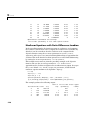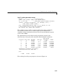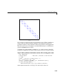
1
Optimization Toolbox For Use with MATLAB ® User’s Guide Version 2 How to Contact The MathWorks: www.mathworks.com comp.soft-sys.matlab Web Newsgroup [email protected] Technical support Product enhancement suggestions Bug reports Documentation error reports Order status, license renewals, passcodes Sales, pricing, and general information 508-647-7000 Phone 508-647-7001 Fax The MathWorks, Inc. 3 Apple Hill Drive Natick, MA 01760-2098 Mail [email protected] [email protected] [email protected] [email protected] [email protected] For contact information about worldwide offices, see the MathWorks Web site. Optimization Toolbox User’s Guide COPYRIGHT 1990 - 2003 by The MathWorks, Inc. The software described in this document is furnished under a license agreement. The software may be used or copied only under the terms of the license agreement. No part of this manual may be photocopied or reproduced in any form without prior written consent from The MathWorks, Inc. FEDERAL ACQUISITION: This provision applies to all acquisitions of the Program and Documentation by or for the federal government of the United States. By accepting delivery of the Program, the government hereby agrees that this software qualifies as "commercial" computer software within the meaning of FAR Part 12.212, DFARS Part 227.7202-1, DFARS Part 227.7202-3, DFARS Part 252.227-7013, and DFARS Part 252.227-7014. The terms and conditions of The MathWorks, Inc. Software License Agreement shall pertain to the government’s use and disclosure of the Program and Documentation, and shall supersede any conflicting contractual terms or conditions. If this license fails to meet the government’s minimum needs or is inconsistent in any respect with federal procurement law, the government agrees to return the Program and Documentation, unused, to MathWorks. MATLAB, Simulink, Stateflow, Handle Graphics, and Real-Time Workshop are registered trademarks, and TargetBox is a trademark of The MathWorks, Inc. Other product or brand names are trademarks or registered trademarks of their respective holders. Printing History: November 1990 December 1996 January 1999 September 2000 June 2001 September 2003 First printing Second printing Third printing Fourth printing Online only Online only For MATLAB 5 For Version 2 (Release 11) For Version 2.1 (Release 12) Revised for Version 2.1.1 (Release 12.1) Revised for Version 2.3 (Release 13SP1) Contents Preface What Is the Optimization Toolbox? . . . . . . . . . . . . . . . . . . . . . viii Related Products . . . . . . . . . . . . . . . . . . . . . . . . . . . . . . . . . . . . . . ix Using This Guide . . . . . . . . . . . . . . . . . . . . . . . . . . . . . . . . . . . . . . xi Configuration Information . . . . . . . . . . . . . . . . . . . . . . . . . . . . . xii Technical Conventions . . . . . . . . . . . . . . . . . . . . . . . . . . . . . . . . xiii Matrix, Vector, and Scalar Notation . . . . . . . . . . . . . . . . . . . . . xiii Typographical Conventions . . . . . . . . . . . . . . . . . . . . . . . . . . . xiv Acknowledgments . . . . . . . . . . . . . . . . . . . . . . . . . . . . . . . . . . . . . xv A Simple Optimization Example 1 Example . . . . . . . . . . . . . . . . . . . . . . . . . . . . . . . . . . . . . . . . . . . . . 1-2 Setting Up the Example . . . . . . . . . . . . . . . . . . . . . . . . . . . . . . . 1-3 Finding the Solution . . . . . . . . . . . . . . . . . . . . . . . . . . . . . . . . . . 1-4 More Examples . . . . . . . . . . . . . . . . . . . . . . . . . . . . . . . . . . . . . . 1-4 i Tutorial 2 Introduction . . . . . . . . . . . . . . . . . . . . . . . . . . . . . . . . . . . . . . . . . . 2-3 Problems Covered by the Toolbox . . . . . . . . . . . . . . . . . . . . . . . . 2-3 Using the Optimization Functions . . . . . . . . . . . . . . . . . . . . . . . 2-5 Examples that Use Standard Algorithms . . . . . . . . . . . . . . . . 2-7 Unconstrained Minimization Example . . . . . . . . . . . . . . . . . . . . 2-8 Nonlinear Inequality Constrained Example . . . . . . . . . . . . . . . 2-9 Constrained Example with Bounds . . . . . . . . . . . . . . . . . . . . . 2-11 Constrained Example with Gradients . . . . . . . . . . . . . . . . . . . 2-12 Gradient Check: Analytic Versus Numeric . . . . . . . . . . . . . . . 2-14 Equality Constrained Example . . . . . . . . . . . . . . . . . . . . . . . . . 2-15 Maximization . . . . . . . . . . . . . . . . . . . . . . . . . . . . . . . . . . . . . . . 2-16 Greater-Than-Zero Constraints . . . . . . . . . . . . . . . . . . . . . . . . 2-16 Additional Arguments: Avoiding Global Variables . . . . . . . . . 2-16 Nonlinear Equations with Analytic Jacobian . . . . . . . . . . . . . . 2-17 Nonlinear Equations with Finite-Difference Jacobian . . . . . . 2-20 Multiobjective Examples . . . . . . . . . . . . . . . . . . . . . . . . . . . . . . 2-21 Large-Scale Examples . . . . . . . . . . . . . . . . . . . . . . . . . . . . . . . . 2-33 Problems Covered by Large-Scale Methods . . . . . . . . . . . . . . . 2-34 Nonlinear Equations with Jacobian . . . . . . . . . . . . . . . . . . . . . 2-37 Nonlinear Equations with Jacobian Sparsity Pattern . . . . . . . 2-40 Nonlinear Least-Squares with Full Jacobian Sparsity Pattern . . . . . . . . . . . . . . . . . . . . . . . . . . . . . . . . . . . . . . . . . . . . 2-42 Nonlinear Minimization with Gradient and Hessian . . . . . . . 2-44 Nonlinear Minimization with Gradient and Hessian Sparsity Pattern . . . . . . . . . . . . . . . . . . . . . . . . . . . . . . . . . . . . . . . . . . . . 2-45 Nonlinear Minimization with Bound Constraints and Banded Preconditioner . . . . . . . . . . . . . . . . . . . . . . . . . . . . . . . . . . . . . . 2-47 Nonlinear Minimization with Equality Constraints . . . . . . . . 2-51 Nonlinear Minimization with a Dense but Structured Hessian and Equality Constraints . . . . . . . . . . . . . . . . . . . . . . . . . . . . . 2-52 Quadratic Minimization with Bound Constraints . . . . . . . . . . 2-56 Quadratic Minimization with a Dense but Structured Hessian . . . . . . . . . . . . . . . . . . . . . . . . . . . . . . . . . . . . . . . . . . . . 2-58 Linear Least-Squares with Bound Constraints . . . . . . . . . . . . 2-61 Linear Programming with Equalities and Inequalities . . . . . . 2-62 ii Contents Linear Programming with Dense Columns in the Equalities . 2-63 Default Parameter Settings . . . . . . . . . . . . . . . . . . . . . . . . . . . 2-66 Changing the Default Settings . . . . . . . . . . . . . . . . . . . . . . . . . 2-66 Displaying Iterative Output . . . . . . . . . . . . . . . . . . . . . . . . . . . 2-69 Output Headings: Medium-Scale Algorithms . . . . . . . . . . . . . 2-69 Output Headings: Large-Scale Algorithms . . . . . . . . . . . . . . . 2-72 Calling an Output Function Iteratively . . . . . . . . . . . . . . . . 2-75 Creating the Output Function . . . . . . . . . . . . . . . . . . . . . . . . . . 2-75 Running the Example . . . . . . . . . . . . . . . . . . . . . . . . . . . . . . . . 2-77 Optimization of Inline Objects Instead of M-Files . . . . . . . 2-80 Typical Problems and How to Deal with Them . . . . . . . . . . 2-82 Selected Bibliography . . . . . . . . . . . . . . . . . . . . . . . . . . . . . . . . 2-86 Standard Algorithms 3 Optimization Overview . . . . . . . . . . . . . . . . . . . . . . . . . . . . . . . . 3-3 Unconstrained Optimization . . . . . . . . . . . . . . . . . . . . . . . . . . . 3-4 Quasi-Newton Methods . . . . . . . . . . . . . . . . . . . . . . . . . . . . . . . . 3-6 Line Search . . . . . . . . . . . . . . . . . . . . . . . . . . . . . . . . . . . . . . . . . . 3-8 Quasi-Newton Implementation . . . . . . . . . . . . . . . . . . . . . . . . . 3-11 Least-Squares Optimization . . . . . . . . . . . . . . . . . . . . . . . . . . . Gauss-Newton Method . . . . . . . . . . . . . . . . . . . . . . . . . . . . . . . Levenberg-Marquardt Method . . . . . . . . . . . . . . . . . . . . . . . . . Nonlinear Least-Squares Implementation . . . . . . . . . . . . . . . . 3-18 3-19 3-20 3-22 Nonlinear Systems of Equations . . . . . . . . . . . . . . . . . . . . . . . 3-24 Gauss-Newton Method . . . . . . . . . . . . . . . . . . . . . . . . . . . . . . . 3-24 iii Trust-Region Dogleg Method . . . . . . . . . . . . . . . . . . . . . . . . . . . 3-24 Nonlinear Equations Implementation . . . . . . . . . . . . . . . . . . . 3-26 Constrained Optimization . . . . . . . . . . . . . . . . . . . . . . . . . . . . Sequential Quadratic Programming (SQP) . . . . . . . . . . . . . . . Quadratic Programming (QP) Subproblem . . . . . . . . . . . . . . . SQP Implementation . . . . . . . . . . . . . . . . . . . . . . . . . . . . . . . . . Simplex Algorithm . . . . . . . . . . . . . . . . . . . . . . . . . . . . . . . . . . . 3-28 3-29 3-30 3-31 3-37 Multiobjective Optimization . . . . . . . . . . . . . . . . . . . . . . . . . . Introduction . . . . . . . . . . . . . . . . . . . . . . . . . . . . . . . . . . . . . . . . Goal Attainment Method . . . . . . . . . . . . . . . . . . . . . . . . . . . . . . Algorithm Improvements for Goal Attainment Method . . . . . 3-42 3-42 3-48 3-49 Selected Bibliography . . . . . . . . . . . . . . . . . . . . . . . . . . . . . . . . 3-52 Large-Scale Algorithms 4 Trust-Region Methods for Nonlinear Minimization . . . . . . . 4-2 Preconditioned Conjugate Gradients . . . . . . . . . . . . . . . . . . . 4-5 Linearly Constrained Problems . . . . . . . . . . . . . . . . . . . . . . . . 4-7 Linear Equality Constraints . . . . . . . . . . . . . . . . . . . . . . . . . . . . 4-7 Box Constraints . . . . . . . . . . . . . . . . . . . . . . . . . . . . . . . . . . . . . . 4-7 Nonlinear Least-Squares . . . . . . . . . . . . . . . . . . . . . . . . . . . . . . 4-10 Quadratic Programming . . . . . . . . . . . . . . . . . . . . . . . . . . . . . . 4-11 Linear Least-Squares . . . . . . . . . . . . . . . . . . . . . . . . . . . . . . . . . 4-12 Large-Scale Linear Programming . . . . . . . . . . . . . . . . . . . . . 4-13 Main Algorithm . . . . . . . . . . . . . . . . . . . . . . . . . . . . . . . . . . . . . 4-13 Preprocessing . . . . . . . . . . . . . . . . . . . . . . . . . . . . . . . . . . . . . . . 4-16 iv Contents Selected Bibliography . . . . . . . . . . . . . . . . . . . . . . . . . . . . . . . . 4-17 Function Reference 5 Functions – By Category . . . . . . . . . . . . . . . . . . . . . . . . . . . . . . . Minimization . . . . . . . . . . . . . . . . . . . . . . . . . . . . . . . . . . . . . . . . Equation Solving . . . . . . . . . . . . . . . . . . . . . . . . . . . . . . . . . . . . . Least Squares (Curve Fitting) . . . . . . . . . . . . . . . . . . . . . . . . . . . Utility . . . . . . . . . . . . . . . . . . . . . . . . . . . . . . . . . . . . . . . . . . . . . . Demos of Large-Scale Methods . . . . . . . . . . . . . . . . . . . . . . . . . . Demos of Medium-Scale Methods . . . . . . . . . . . . . . . . . . . . . . . . 5-2 5-2 5-2 5-3 5-3 5-3 5-4 Function Arguments . . . . . . . . . . . . . . . . . . . . . . . . . . . . . . . . . . 5-5 Input Arguments . . . . . . . . . . . . . . . . . . . . . . . . . . . . . . . . . . . . . 5-5 Output Arguments . . . . . . . . . . . . . . . . . . . . . . . . . . . . . . . . . . . . 5-8 Optimization Parameters . . . . . . . . . . . . . . . . . . . . . . . . . . . . . 5-10 Output Function . . . . . . . . . . . . . . . . . . . . . . . . . . . . . . . . . . . . . 5-15 Structure of the Output Function . . . . . . . . . . . . . . . . . . . . . . . 5-15 Functions — Alphabetical List . . . . . . . . . . . . . . . . . . . . . . . . 5-24 Index v vi Contents Preface The Preface consists of these sections: What Is the Optimization Toolbox? (p. viii) Introduces the Optimization Toolbox, and describes its intended use and its capabilities. Related Products (p. ix) Lists products that are relevant to the kinds of tasks you can perform with the Optimization Toolbox. Using This Guide (p. xi) Explains the organization of this guide. Configuration Information (p. xii) Directs you to installation and configuration information. Technical Conventions (p. xiii) Describes mathematical notation used in this guide. Typographical Conventions (p. xiv) Describes the typographical conventions used in this guide. Acknowledgments (p. xv) Acknowledges significant contributions to the Optimization Toolbox. Preface What Is the Optimization Toolbox? The Optimization Toolbox is a collection of functions that extend the capability of the MATLAB® numeric computing environment. The toolbox includes routines for many types of optimization including • Unconstrained nonlinear minimization • Constrained nonlinear minimization, including goal attainment problems, minimax problems, and semi-infinite minimization problems • Quadratic and linear programming • Nonlinear least squares and curve-fitting • Nonlinear system of equation solving • Constrained linear least squares • Sparse and structured large-scale problems All the toolbox functions are MATLAB M-files, made up of MATLAB statements that implement specialized optimization algorithms. You can view the MATLAB code for these functions using the statement type function_name You can extend the capabilities of the Optimization Toolbox by writing your own M-files, or by using the toolbox in combination with other toolboxes, or with MATLAB or Simulink®. viii Related Products Related Products The MathWorks provides several products that are relevant to the kinds of tasks you can perform with the Optimization Toolbox. For more information about any of these products, see either • The online documentation for that product, if it is installed or if you are reading the documentation from the CD • The MathWorks Web site, at http://www.mathworks.com; see the “products” section Note The following toolboxes all include functions that extend the MATLAB capabilities. The blocksets all include blocks that extend Simulink’s capabilities. Product Description Curve Fitting Toolbox Perform model fitting and analysis Data Acquisition Toolbox Acquire and send out data from plug-in data acquisition boards Database Toolbox Exchange data with relational databases Financial Time Series Toolbox Analyze and manage financial time-series data Financial Toolbox Model financial data and develop financial analysis algorithms GARCH Toolbox Analyze financial volatility using univariate GARCH models LMI Control Toolbox Design robust controllers using convex optimization techniques Neural Network Toolbox Design and simulate neural networks ix Preface x Product Description Nonlinear Control Design Blockset Optimize design parameters in nonlinear control systems Signal Processing Toolbox Perform signal processing, analysis, and algorithm development Simulink Design and simulate continuous- and discrete-time systems Spline Toolbox Create and manipulate spline approximation models of data Statistics Toolbox Apply statistical algorithms and probability models Symbolic/Extended Symbolic Math Toolbox Perform computations using symbolic mathematics and variable-precision arithmetic System Identification Toolbox Create linear dynamic models from measured input-output data Using This Guide Using This Guide This guide has the following chapters: • “A Simple Optimization Example” provides an example to help you get started with the Optimization Toolbox. • The “Tutorial” chapter shows you how to solve a variety of different optimization problems. It includes a section that highlights large-scale problems. This chapter also provides information on how to use the toolbox functions in conjunction with Simulink using multiobjective optimization. Other sections include information about changing default parameters and using inline objects. • The “Standard Algorithms” and “Large-Scale Algorithms” chapters describe the algorithms used by the optimization functions. “Standard Algorithms” describes the problem formulations and algorithms for the medium-scale algorithms. “Large-Scale Algorithms” focuses on algorithms used to solve large sparse or structured problems. • The “Function Reference” chapter provides a detailed reference description of each toolbox function. Reference descriptions include the function’s syntax, a description of the different calling sequences available, and detailed information about arguments to the function, including relevant optimization options parameters. Reference descriptions can also include examples, a summary of the function’s algorithms, and references to additional reading material. xi Preface Configuration Information To determine whether the Optimization Toolbox is installed on your system, type this command at the MATLAB prompt. ver When you enter this command, MATLAB displays information about the version of MATLAB you are running, including a list of all toolboxes installed on your system and their version numbers. If the Optimization Toolbox is not installed, check the Installation documentation for your platform for instructions on how to install it. Note For the most up-to-date information about system requirements, see the individual product pages at the MathWorks Web site (http://www.mathworks.com). xii Technical Conventions Technical Conventions Matrix, Vector, and Scalar Notation Uppercase letters such as A are used to denote matrices. Lowercase letters such as x are used to denote vectors, except where noted that the variable is a scalar. For functions, the notation differs slightly to follow the usual conventions in optimization. For vector functions, we use an upper-case letter such as F in F ( x ) . A function that returns a scalar value is denoted with a lowercase letter such as f in f ( x ) . xiii Preface Typographical Conventions This manual uses some or all of these conventions. Item Convention Example Example code Monospace font To assign the value 5 to A, enter A = 5 Function names, syntax, filenames, directory/folder names, and user input Monospace font The cos function finds the cosine of each array element. Syntax line example is MLGetVar ML_var_name Buttons and keys Boldface with book title caps Press the Enter key. Literal strings (in syntax descriptions in reference chapters) Monospace bold for literals f = freqspace(n,'whole') Mathematical expressions Italic for variables This vector represents the polynomial p = x2 + 2x + 3. MATLAB output Monospace font Standard text font for functions, operators, and constants MATLAB responds with A = 5 xiv Menu and dialog box titles Boldface with book title caps Choose the File Options menu. New terms and for emphasis Italic An array is an ordered collection of information. Omitted input arguments (...) ellipsis denotes all of the input/output arguments from preceding syntaxes. [c,ia,ib] = union(...) String variables (from a finite list) Monospace italic sysc = d2c(sysd,'method') Acknowledgments Acknowledgments The MathWorks would like to acknowledge these contributors: Thomas F. Coleman researched and contributed the large-scale algorithms for constrained and unconstrained minimization, nonlinear least squares and curve fitting, constrained linear least squares, quadratic programming, and nonlinear equations. Dr. Coleman is Professor of Computer Science and Applied Mathematics at Cornell University. He is Director of the Cornell Theory Center and the Cornell Computational Finance Institute. Dr. Coleman is Chair of the SIAM Activity Group on Optimization, and a member of the Editorial Boards of Applied Mathematics Letters, SIAM Journal of Scientific Computing, Computational Optimization and Applications, Communications on Applied Nonlinear Analysis, and Mathematical Modeling and Scientific Computing. Dr. Coleman has published 4 books and over 70 technical papers in the areas of continuous optimization and computational methods and tools for large-scale problems. Yin Zhang researched and contributed the large-scale linear programming algorithm. Dr. Zhang is Associate Professor of Computational and Applied Mathematics on the faculty of the Keck Center for Computational Biology at Rice University. He is on the Editorial Board of SIAM Journal on Optimization, and is Associate Editor of Journal of Optimization: Theory and Applications. Dr. Zhang has published over 40 technical papers in the areas of interior-point methods for linear programming and computation mathematical programming. xv Preface xvi 1 A Simple Optimization Example This section presents a simple example to help you get started using the Optimization Toolbox. Example (p. 1-2) Introduces the example. Setting Up the Example (p. 1-3) Shows how to set up the problem before applying the optimization function. Finding the Solution (p. 1-4) Shows how to solve the problem using the linear least squares optimization function lsqlin. 1 A Simple Optimization Example Example Suppose you want to find the point on the plane x 1 + 2x 2 + 4x 3 = 7 that is closest to the origin. The easiest way to solve this problem is to minimize the square of the distance from a point x = ( x 1, x 2, x 3 ) on the plane to the origin. This returns the same optimal point as minimizing the actual distance. You can describe the problem of minimizing the square of the distance as follows: 2 2 2 minimize f ( x ) = x 1 + x 2 + x 3 x subject to the constraint x 1 + 2x 2 + 4x 3 = 7 The function f(x) is called the objective function and x 1 + 2x 2 + 4x 3 = 7 is an equality constraint. More complicated problems might contain other equality constraints, inequality constraints, and upper or lower bound constraints. This example uses the linear least squares function lsqlin to solve the problem. 1-2 Setting Up the Example Setting Up the Example This section shows how to set up the example before applying the function lsqlin, which solves linear least squares problems of the form minimize f ( x ) = Cx – d x where Cx – d 2 2 is the norm of Cx - d squared, subject to the contraints Ax ≤ b Aeq ⋅ x = beq To set up the problem, you must create variables for the parameters C, d, A, b, Aeq, and beq. lsqlin accepts these variables as input arguments with the following syntax: x = lsqlin(C, d, A, b, Aeq, beq) To create the variables, do the following steps: 1. Create Variables for the Objective Function 2 2 2 2 Since you want to minimize x 1 + x 2 + x 3 = x , you can set C to be the 3-by-3 identity matrix and d to be a 3-by-1 vector of zeros, so that Cx - d = x. C = eye(3); d = zeros(3,1); 2. Create Variables for the Constraints Since this examples has no inequality constraints, you can set A and b to be empty matrices in the input arguments. You can represent the equality constraint x 1 + 2x 2 + 4x 3 = 7 in matrix form as Aeq ⋅ x = beq where Aeq = [1 2 4] and beq = [7]. To create variables for Aeq and beq, enter Aeq = [1 2 4]; beq = [7]; 1-3 1 A Simple Optimization Example Finding the Solution To solve the optimization problem, enter [x, fval] =lsqlin(C, d, [], [], Aeq, beq) lsqlin returns x = 0.3333 0.6667 1.3333 fval = 2.3333 The minimum occurs at the point x and fval is the square of the distance from x to the origin. Note In this example, lsqlin issues a warning that it is switching from its default large-scale algorithm to its medium-scale algorithm. This message has no bearing on the result, so you can safely ignore it. “Using the Optimization Functions” on page 2-5 provides more information on large and medium-scale algorithms. More Examples The following sections contain more examples of solving optimization problems: • “Examples that Use Standard Algorithms” on page 2-7 • “Large-Scale Examples” on page 2-33 1-4 2 Tutorial The Tutorial provides information on how to use the toolbox functions. It also provides examples for solving different optimization problems. It consists of these sections. Introduction (p. 2-3) Summarizes, in tabular form, the functions available for minimization, equation solving, and solving least-squares or data fitting problems. It also provides basic guidelines for using the optimization routines and introduces the algorithms and line-search strategies that are available for solving medium- and large-scale problems. Examples that Use Standard Algorithms (p. 2-7) Presents medium-scale algorithms through a selection of minimization examples. These examples include unconstrained and constrained problems, as well as problems with and without user-supplied gradients. This section also discusses maximization, greater-than-zero constraints, passing additional arguments, and multiobjective examples. Large-Scale Examples (p. 2-33) Presents large-scale algorithms through a selection of large-scale examples. These examples include specifying sparsity structures, and preconditioners, as well as unconstrained and constrained problems. Default Parameter Settings (p. 2-66) Describes the use of default parameter settings and tells you how to change them. It also tells you how to determine which parameters are used by a specified function, and provides examples of setting some commonly used parameters. Displaying Iterative Output (p. 2-69) Describes the column headings used in the iterative output of both medium-scale and large-scale algorithms. Calling an Output Function Iteratively Describes how to make an optimization function call an (p. 2-75) output function at each iteration. 2 Tutorial 2-2 Optimization of Inline Objects Instead of M-Files (p. 2-80) Tells you how to represent a mathematical function at the command line by creating an inline object from a string expression. Typical Problems and How to Deal with Them (p. 2-82) Provides tips to help you improve solutions found using the optimization functions, improve efficiency of the algorithms, overcome common difficulties, and transform problems that are typically not in standard form. Selected Bibliography (p. 2-86) Lists published materials that support concepts implemented in the Optimization Toolbox. Introduction Introduction Optimization concerns the minimization or maximization of functions. The Optimization Toolbox consists of functions that perform minimization (or maximization) on general nonlinear functions. Functions for nonlinear equation solving and least-squares (data-fitting) problems are also provided. This introduction includes the following sections: • Problems Covered by the Toolbox • Using the Optimization Functions Problems Covered by the Toolbox The following tables show the functions available for minimization, equation solving, and solving least-squares or data-fitting problems. Note The following tables list the types of problems in order of increasing complexity. Table 2-1: Minimization Type Notation Function Scalar Minimization min f ( a ) such that a 1 ≤ a ≤ a 2 a fminbnd Unconstrained Minimization min f ( x ) x fminunc, fminsearch Linear Programming min f x such that x A ⋅ x ≤ b, Aeq ⋅ x = beq, l ≤ x ≤ u Quadratic Programming T 1 T min --- x Hx + f x such that x 2 A ⋅ x ≤ b, Aeq ⋅ x = beq, l ≤ x ≤ u T linprog quadprog 2-3 2 Tutorial Table 2-1: Minimization (Continued) Type Notation Function Constrained Minimization min f ( x ) such that x c ( x ) ≤ 0, ceq ( x ) = 0 fmincon A ⋅ x ≤ b, Aeq ⋅ x = beq, l ≤ x ≤ u Goal Attainment min γ such that x, γ F ( x ) – wγ ≤ goal fgoalattain c ( x ) ≤ 0, ceq ( x ) = 0 A ⋅ x ≤ b, Aeq ⋅ x = beq, l ≤ x ≤ u Minimax min max { F i(x) } x {F } i such that fminimax c ( x ) ≤ 0, ceq ( x ) = 0 A ⋅ x ≤ b, Aeq ⋅ x = beq, l ≤ x ≤ u Semi-Infinite Minimization min f ( x ) such that x K(x, w) ≤ 0 for all w fseminf c ( x ) ≤ 0, ceq ( x ) = 0 A ⋅ x ≤ b, Aeq ⋅ x = beq, l ≤ x ≤ u Table 2-2: Equation Solving 2-4 Type Notation Function Linear Equations C ⋅ x = d , n equations, n variables \ (slash) Nonlinear Equation of One Variable f( a) = 0 fzero Nonlinear Equations F(x) = 0 , n equations, n variables fsolve Introduction Table 2-3: Least-Squares (Curve Fitting) Type Notation Linear Least-Squares min C ⋅ x – d 2 , m equations, n variables x Nonnegative Linear-Least-Squares min C ⋅ x – d 2 x Constrained Linear-Least-Squares such that min C ⋅ x – d 2 x A ⋅ x ≤ b, Aeq ⋅ x = beq, l ≤ x ≤ u Nonlinear Least-Squares Nonlinear Curve Fitting Function 2 2 such that x ≥ 0 2 2 2 1 1 min --- F(x) 2 = --Fi ( x) 2 x 2 i 2 1 min --- F(x, xdata) – ydata 2 2 x ∑ \ (slash) lsqnonneg lsqlin such that l ≤ x ≤ u lsqnonlin such that l ≤ x ≤ u lsqcurvefit Using the Optimization Functions Most of these optimization routines require the definition of an M-file containing the function to be minimized, i.e., the objective function. Alternatively, you can use an inline object created from a MATLAB expression. Maximization is achieved by supplying the routines with -f, where f is the function being optimized. Optimization options passed to the routines change optimization parameters. Default optimization parameters are used extensively but can be changed through an options structure. Gradients are calculated using an adaptive finite-difference method unless they are supplied in a function. Parameters can be passed directly to functions, avoiding the need for global variables. This guide separates “medium-scale” algorithms from “large-scale” algorithms. Medium-scale is not a standard term and is used here only to differentiate these algorithms from the large-scale algorithms, which are designed to handle large-scale problems efficiently. 2-5 2 Tutorial Medium-Scale Algorithms The Optimization Toolbox routines offer a choice of algorithms and line search strategies. The principal algorithms for unconstrained minimization are the Nelder-Mead simplex search method and the BFGS (Broyden, Fletcher, Goldfarb, and Shanno) quasi-Newton method. For constrained minimization, minimax, goal attainment, and semi-infinite optimization, variations of sequential quadratic programming (SQP) are used. Nonlinear least-squares problems use the Gauss-Newton and Levenberg-Marquardt methods. Nonlinear equation solving also uses the trust-region dogleg algorithm. A choice of line search strategy is given for unconstrained minimization and nonlinear least-squares problems. The line search strategies use safeguarded cubic and quadratic interpolation and extrapolation methods. Large-Scale Algorithms All the large-scale algorithms, except linear programming, are trust-region methods. Bound constrained problems are solved using reflective Newton methods. Equality constrained problems are solved using a projective preconditioned conjugate gradient iteration. You can use sparse iterative solvers or sparse direct solvers in solving the linear systems to determine the current step. Some choice of preconditioning in the iterative solvers is also available. The linear programming method is a variant of Mehrotra’s predictor-corrector algorithm, a primal-dual interior-point method. 2-6 Examples that Use Standard Algorithms Examples that Use Standard Algorithms This section presents the medium-scale (i.e., standard) algorithms through a tutorial. Examples similar to those in the first part of this tutorial (“Unconstrained Minimization Example” through the “Equality Constrained Example”) can also be found in the first demonstration, “Tutorial Walk Through,” in the M-file optdemo. The examples in this manual differ in that they use M-file functions for the objective functions, whereas the online demonstrations use inline objects for some functions. Note Medium-scale is not a standard term and is used to differentiate these algorithms from the large-scale algorithms described in “Large-Scale Algorithms” on page 4-1. The tutorial uses the functions fminunc, fmincon, and fsolve. The other optimization routines, fgoalattain, fminimax, lsqnonlin, and fseminf, are used in a nearly identical manner, with differences only in the problem formulation and the termination criteria. The section “Multiobjective Examples” on page 2-21 discusses multiobjective optimization and gives several examples using lsqnonlin, fminimax, and fgoalattain, including how Simulink can be used in conjunction with the toolbox. This section includes the following examples: • Unconstrained Minimization Example • Nonlinear Inequality Constrained Example • Constrained Example with Bounds • Constrained Example with Gradients • Gradient Check: Analytic Versus Numeric • Equality Constrained Example It also discusses • Maximization • Greater-Than-Zero Constraints • Additional Arguments: Avoiding Global Variables • Nonlinear Equations with Analytic Jacobian 2-7 2 Tutorial • Nonlinear Equations with Finite-Difference Jacobian • Multiobjective Examples Unconstrained Minimization Example Consider the problem of finding a set of values [x1, x2] that solves x1 2 2 minimize f ( x ) = e ( 4x 1 + 2x 2 + 4x 1 x 2 + 2x 2 + 1 ) x (2-1) To solve this two-dimensional problem, write an M-file that returns the function value. Then, invoke the unconstrained minimization routine fminunc. Step 1: Write an M-file objfun.m. function f = objfun(x) f = exp(x(1))*(4*x(1)^2+2*x(2)^2+4*x(1)*x(2)+2*x(2)+1); Step 2: Invoke one of the unconstrained optimization routines. x0 = [-1,1]; % Starting guess options = optimset('LargeScale','off'); [x,fval,exitflag,output] = fminunc(@objfun,x0,options); After 40 function evaluations, this produces the solution x = 0.5000 -1.0000 The function at the solution x is returned in fval: fval = 1.3030e-10 The exitflag tells whether the algorithm converged. An exitflag > 0 means a local minimum was found: exitflag = 1 The output structure gives more details about the optimization. For fminunc, it includes the number of iterations in iterations, the number of function evaluations in funcCount, the final step-size in stepsize, a measure of first-order optimality (which in this unconstrained case is the infinity norm of 2-8 Examples that Use Standard Algorithms the gradient at the solution) in firstorderopt, and the type of algorithm used in algorithm: output = iterations: funcCount: stepsize: firstorderopt: algorithm: 7 40 1 9.2801e-004 'medium-scale: Quasi-Newton line search' When more than one local minimum exists, the initial guess for the vector [x1, x2] affects both the number of function evaluations and the value of the solution point. In the preceding example, x0 is initialized to [-1,1]. The variable options can be passed to fminunc to change characteristics of the optimization algorithm, as in x = fminunc(@objfun,x0,options); options is a structure that contains values for termination tolerances and algorithm choices. An options structure can be created using the optimset function: options = optimset('LargeScale','off'); In this example, we have turned off the default selection of the large-scale algorithm and so the medium-scale algorithm is used. Other options include controlling the amount of command line display during the optimization iteration, the tolerances for the termination criteria, whether a user-supplied gradient or Jacobian is to be used, and the maximum number of iterations or function evaluations. See optimset, the individual optimization functions, and Table , Optimization Parameters, on page 5-28 for more options and information. Nonlinear Inequality Constrained Example If inequality constraints are added to Eq. 2-1, the resulting problem can be solved by the fmincon function. For example, find x that solves x 2 2 minimize f ( x ) = e 1 ( 4x 1 + 2x 2 + 4x 1 x 2 + 2x 2 + 1 ) x (2-2) subject to the constraints 2-9 2 Tutorial x 1 x 2 – x 1 – x 2 ≤ – 1.5 x 1 x 2 ≥ – 10 Because neither of the constraints is linear, you cannot pass the constraints to fmincon at the command line. Instead you can create a second M-file, confun.m, that returns the value at both constraints at the current x in a vector c. The constrained optimizer, fmincon, is then invoked. Because fmincon expects the constraints to be written in the form c ( x ) ≤ 0 , you must rewrite your constraints in the form x 1 x 2 – x 1 – x 2 + 1.5 ≤ 0 – x 1 x 2 – 10 ≤ 0 (2-3) Step 1: Write an M-file confun.m for the constraints. function [c, ceq] = confun(x) % Nonlinear inequality constraints c = [1.5 + x(1)*x(2) - x(1) - x(2); -x(1)*x(2) - 10]; % Nonlinear equality constraints ceq = []; Step 2: Invoke constrained optimization routine. x0 = [-1,1]; % Make a starting guess at the solution options = optimset('LargeScale','off'); [x, fval] = ... fmincon(@objfun,x0,[],[],[],[],[],[],@confun,options) After 38 function calls, the solution x produced with function value fval is x = -9.5474 fval = 0.0236 1.0474 We can evaluate the constraints at the solution [c,ceq] = confun(x) c= 1.0e-14 * 0.1110 2-10 Examples that Use Standard Algorithms -0.1776 ceq = [] Note that both constraint values are less than or equal to zero; that is, x satisfies c ( x ) ≤ 0 . Constrained Example with Bounds The variables in x can be restricted to certain limits by specifying simple bound constraints to the constrained optimizer function. For fmincon, the command x = fmincon(@objfun,x0,[],[],[],[],lb,ub,@confun,options); limits x to be within the range lb <= x <= ub. To restrict x in Eq. 2-2 to be greater than zero (i.e., x 1 ≥ 0 , x 2 ≥ 0 ), use the commands x0 = [-1,1]; % Make a starting guess at the solution lb = [0,0]; % Set lower bounds ub = [ ]; % No upper bounds options = optimset('LargeScale','off'); [x,fval = ... fmincon(@objfun,x0,[],[],[],[],lb,ub,@confun,options) [c, ceq] = confun(x) Note that to pass in the lower bounds as the seventh argument to fmincon, you must specify values for the third through sixth arguments. In this example, we specified [] for these arguments since there are no linear inequalities or linear equalities. After 13 function evaluations, the solution produced is x = 0 1.5000 fval = 8.5000 c = 0 -10 ceq = 2-11 2 Tutorial [] When lb or ub contains fewer elements than x, only the first corresponding elements in x are bounded. Alternatively, if only some of the variables are bounded, then use -inf in lb for unbounded below variables and inf in ub for unbounded above variables. For example, lb = [-inf 0]; ub = [10 inf]; bounds x 1 ≤ 10 , 0 ≤ x 2 ( x 1 has no lower bound and x 2 has no upper bound). Using inf and -inf give better numerical results than using a very large positive number or a very large negative number to imply lack of bounds. Note that the number of function evaluations to find the solution is reduced because we further restricted the search space. Fewer function evaluations are usually taken when a problem has more constraints and bound limitations because the optimization makes better decisions regarding step size and regions of feasibility than in the unconstrained case. It is, therefore, good practice to bound and constrain problems, where possible, to promote fast convergence to a solution. Constrained Example with Gradients Ordinarily the medium-scale minimization routines use numerical gradients calculated by finite-difference approximation. This procedure systematically perturbs each of the variables in order to calculate function and constraint partial derivatives. Alternatively, you can provide a function to compute partial derivatives analytically. Typically, the problem is solved more accurately and efficiently if such a function is provided. To solve Eq. 2-2 using analytically determined gradients, do the following. Step 1: Write an M-file for the objective function and gradient. function [f,G] = objfungrad(x) f = exp(x(1))*(4*x(1)^2+2*x(2)^2+4*x(1)*x(2)+2*x(2)+1); % Gradient of the objective function t = exp(x(1))*(4*x(1)^2+2*x(2)^2+4*x(1)*x(2)+2*x(2)+1); G = [ t + exp(x(1)) * (8*x(1) + 4*x(2)), exp(x(1))*(4*x(1)+4*x(2)+2)]; 2-12 Examples that Use Standard Algorithms Step 2: Write an M-file for the nonlinear constraints and the gradients of the nonlinear constraints. function [c,ceq,DC,DCeq] = confungrad(x) c(1) = 1.5 + x(1) * x(2) - x(1) - x(2); %Inequality constraints c(2) = -x(1) * x(2)-10; % Gradient of the constraints DC= [x(2)-1, -x(2); x(1)-1, -x(1)]; % No nonlinear equality constraints ceq=[]; DCeq = [ ]; G contains the partial derivatives of the objective function, f, returned by objfungrad(x), with respect to each of the elements in x: x1 ∂f ----- = ∂x 2 x1 2 e ( 4x 1 + 2x 2 + 4x 1 x 2 + 2x 2 + 1 ) + e ( 8x 1 + 4x 2 ) (2-4) x1 e ( 4x 1 + 4x 2 + 2 ) The columns of DC contain the partial derivatives for each respective constraint (i.e., the ith column of DC is the partial derivative of the ith constraint with respect to x). So in the above example, DC is ∂c 1 -------∂x 1 ∂c 2 -------∂x 1 x2 – 1 –x2 = ∂c 1 -------∂x 2 ∂c 2 -------∂x 2 (2-5) x1 – 1 –x1 Since you are providing the gradient of the objective in objfungrad.m and the gradient of the constraints in confungrad.m, you must tell fmincon that these M-files contain this additional information. Use optimset to turn the parameters GradObj and GradConstr to 'on' in the example’s existing options structure: options = optimset(options,'GradObj','on','GradConstr','on'); 2-13 2 Tutorial If you do not set these parameters to 'on' in the options structure, fmincon does not use the analytic gradients. The arguments lb and ub place lower and upper bounds on the independent variables in x. In this example, there are no bound constraints and so they are both set to []. Step 3: Invoke constrained optimization routine. x0 = [-1,1]; % Starting guess options = optimset('LargeScale','off'); options = optimset(options,'GradObj','on','GradConstr','on'); lb = [ ]; ub = [ ]; % No upper or lower bounds [x,fval] = fmincon(@objfungrad,x0,[],[],[],[],lb,ub,... @confungrad,options) [c,ceq] = confungrad(x) % Check the constraint values at x After 20 function evaluations, the solution produced is x = -9.5474 1.0474 fval = 0.0236 c = 1.0e-14 * 0.1110 -0.1776 ceq = [] Gradient Check: Analytic Versus Numeric When analytically determined gradients are provided, you can compare the supplied gradients with a set calculated by finite-difference evaluation. This is particularly useful for detecting mistakes in either the objective function or the gradient function formulation. If you want such gradient checks, set the DerivativeCheck parameter to 'on' using optimset: options = optimset(options,'DerivativeCheck','on'); 2-14 Examples that Use Standard Algorithms The first cycle of the optimization checks the analytically determined gradients (of the objective function and, if they exist, the nonlinear constraints). If they do not match the finite-differencing gradients within a given tolerance, a warning message indicates the discrepancy and gives the option to abort the optimization or to continue. Equality Constrained Example For routines that permit equality constraints, nonlinear equality constraints must be computed in the M-file with the nonlinear inequality constraints. For linear equalities, the coefficients of the equalities are passed in through the matrix Aeq and the right-hand-side vector beq. 2 For example, if you have the nonlinear equality constraint x 1 + x 2 = 1 and the nonlinear inequality constraint x 1 x 2 ≥ – 10 , rewrite them as 2 x1 + x2 – 1 = 0 – x 1 x 2 – 10 ≤ 0 and then solve the problem using the following steps. Step 1: Write an M-file objfun.m. function f = objfun(x) f = exp(x(1))*(4*x(1)^2+2*x(2)^2+4*x(1)*x(2)+2*x(2)+1); Step 2: Write an M-file confuneq.m for the nonlinear constraints. function [c, ceq] = confuneq(x) % Nonlinear inequality constraints c = -x(1)*x(2) - 10; % Nonlinear equality constraints ceq = x(1)^2 + x(2) - 1; Step 3: Invoke constrained optimization routine. x0 = [-1,1]; % Make a starting guess at the solution options = optimset('LargeScale','off'); [x,fval] = fmincon(@objfun,x0,[],[],[],[],[],[],... @confuneq,options) [c,ceq] = confuneq(x) % Check the constraint values at x 2-15 2 Tutorial After 21 function evaluations, the solution produced is x = -0.7529 0.4332 fval = 1.5093 c = -9.6739 ceq = 4.0684e-010 Note that ceq is equal to 0 within the default tolerance on the constraints of 1.0e-006 and that c is less than or equal to zero as desired. Maximization The optimization functions fminbnd, fminsearch, fminunc, fmincon, fgoalattain, fminimax, lsqcurvefit, and lsqnonlin all perform minimization of the objective function f ( x ) . Maximization is achieved by supplying the routines with – f ( x ) . Similarly, to achieve maximization for quadprog supply -H and -f, and for linprog supply -f. Greater-Than-Zero Constraints The Optimization Toolbox assumes that nonlinear inequality constraints are of the form C i ( x ) ≤ 0 . Greater-than-zero constraints are expressed as less-than-zero constraints by multiplying them by -1. For example, a constraint of the form C i ( x ) ≥ 0 is equivalent to the constraint ( – C i ( x ) ) ≤ 0 ; a constraint of the form C i ( x ) ≥ b is equivalent to the constraint ( – C i ( x ) + b ) ≤ 0 . Additional Arguments: Avoiding Global Variables You can pass parameters that would otherwise have to be declared as global directly to M-file functions using additional arguments at the end of the calling sequence. For example, entering a number of variables at the end of the call to fsolve [x,fval] = fsolve(@objfun,x0,options,P1,P2,...) passes the arguments directly to the function objfun when it is called from inside fsolve: 2-16 Examples that Use Standard Algorithms F = objfun(x,P1,P2, ... ) Consider, for example, finding zeros of the function ellipj(u,m). The function needs parameter m as well as input u. To look for a zero near u = 3, for m = 0.5, m = 0.5; options = optimset('Display','off'); % Turn off Display x = fsolve(@ellipj,3,options,m) returns x = 3.7081 Then, solve for the function ellipj: f = ellipj(x,m) f = -2.9925e-008 The call to optimset to get the default options for fsolve implies that default tolerances are used and that analytic gradients are not provided. Nonlinear Equations with Analytic Jacobian This example demonstrates the use of the default medium-scale fsolve algorithm. It is intended for problems where • The system of nonlinear equations is square, i.e., the number of equations equals the number of unknowns. • There exists a solution x such that F ( x ) = 0 . The example uses fsolve to obtain the minimum of the banana (or Rosenbrock) function by deriving and then solving an equivalent system of nonlinear equations. The Rosenbrock function, which has a minimum at F ( x ) = 0 , is a common test problem in optimization. It has a high degree of nonlinearity and converges extremely slowly if you try to use steepest descent type methods. It is given by 2 2 f ( x ) = 100 ( x 2 – x 1 ) + ( 1 – x 1 ) 2 First generalize this function to an n-dimensional function, for any positive, even value of n: 2-17 2 Tutorial n⁄2 f( x) = ∑ 100 ( x2i – x2i – 1 ) 2 2 + ( 1 – x 2i – 1 ) 2 i=1 This function is referred to as the generalized Rosenbrock function. It consists of n squared terms involving n unknowns. Before you can use fsolve to find the values of x such that F ( x ) = 0 , i.e., obtain the minimum of the generalized Rosenbrock function, you must rewrite the function as the following equivalent system of nonlinear equations: F ( 1 ) = 1 – x1 2 F ( 2 ) = 10 ( x 2 – x 1 ) F ( 3 ) = 1 – x3 2 F ( 4 ) = 10 ( x 4 – x 3 ) .. . F ( n – 1 ) = 1 – xn – 1 2 F ( n ) = 10 ( x n – x n – 1 ) This system is square, and you can use fsolve to solve it. As the example demonstrates, this system has a unique solution given by x i = 1, i = 1, …, n . Step 1: Write an M-file bananaobj.m to compute the objective function values and the Jacobian. function [F,J] = bananaobj(x); % Evaluate the vector function and the Jacobian matrix for % the system of nonlinear equations derived from the general % n-dimensional Rosenbrock function. % Get the problem size n = length(x); if n == 0, error('Input vector, x, is empty.'); end if mod(n,2) ~= 0, error('Input vector, x, must have an even number of components.'); end 2-18 Examples that Use Standard Algorithms % Evaluate the vector function odds = 1:2:n; evens = 2:2:n; F = zeros(n,1); F(odds,1) = 1-x(odds); F(evens,1) = 10.*(x(evens)-x(odds).^2); % Evaluate the Jacobian matrix if nargout > 1 if nargout > 1 c = -ones(n/2,1); C = sparse(odds,odds,c,n,n); d = 10*ones(n/2,1); D = sparse(evens,evens,d,n,n); e = -20.*x(odds); E = sparse(evens,odds,e,n,n); J = C + D + E; end Step 2: Call the solve routine for the system of equations. n = 64; x0(1:n,1) = -1.9; x0(2:2:n,1) = 2; options=optimset('Display','iter','Jacobian','on'); [x,F,exitflag,output,JAC] = fsolve(@bananaobj,x0,options); Use the starting point x ( i ) = – 1.9 for the odd indices, and x ( i ) = 2 for the even indices. Accept the fsolve default 'off' for the LargeScale parameter, and the default medium-scale nonlinear equation algorithm 'dogleg'. Then set Jacobian to 'on' to use the Jacobian defined in bananaobj.m . The fsolve function generates the following output: Iteration Func-count f(x) 0 1 4281.92 1 2 1546.86 2 3 112.552 3 4 106.24 4 5 106.24 5 6 51.3854 6 7 51.3854 7 8 43.8722 8 9 37.0713 9 10 37.0713 10 11 26.2485 Norm of First-order Trust-region step optimality radius 615 1 1 329 1 2.5 34.8 2.5 6.25 34.1 6.25 6.25 34.1 6.25 1.5625 6.39 1.56 3.90625 6.39 3.91 0.976562 2.19 0.977 2.44141 6.27 2.44 2.44141 6.27 2.44 0.610352 1.52 0.61 2-19 2 Tutorial 11 12 20.6649 1.52588 4.63 12 13 17.2558 1.52588 6.97 13 14 8.48582 1.52588 4.69 14 15 4.08398 1.52588 3.77 15 16 1.77589 1.52588 3.56 16 17 0.692381 1.52588 3.31 17 18 0.109777 1.16206 1.66 18 19 0 0.0468565 0 Optimization terminated successfully: First-order optimality is less than options.TolFun 1.53 1.53 1.53 1.53 1.53 1.53 1.53 1.53 Nonlinear Equations with Finite-Difference Jacobian In the preceding example, the function bananaobj evaluates F and computes the Jacobian J. What if the code to compute the Jacobian is not available? By default, if you do not indicate that the Jacobian can be computed in the objective function (using the Jacobian parameter in options), fsolve, lsqnonlin, and lsqcurvefit instead use finite differencing to approximate the Jacobian. This is the default Jacobian option.You can select finite differencing by setting the Jacobian parameter to 'off' in optimset. This example uses bananaobj from the preceding example as the objective function, but sets the Jacobian parameter to 'off' so that fsolve approximates the Jacobian and ignores the second bananaobjoutput. It accepts the fsolve default 'off' for the LargeScale parameter, and the default nonlinear equation medium-scale algorithm 'dogleg': n = 64; x0(1:n,1) = -1.9; x0(2:2:n,1) = 2; options=optimset('Display','iter','Jacobian','off'); [x,F,exitflag,output,JAC] = fsolve(@bananaobj,x0,options); The example produces the following output: Iteration Func-count f(x) 0 65 4281.92 1 130 1546.86 2 195 112.552 3 260 106.24 4 261 106.24 2-20 Norm of First-order Trust-region step optimality radius 615 1 1 329 1 2.5 34.8 2.5 6.25 34.1 6.25 6.25 34.1 6.25 Examples that Use Standard Algorithms 5 326 51.3854 1.5625 6.39 6 327 51.3854 3.90625 6.39 7 392 43.8722 0.976562 2.19 8 457 37.0713 2.44141 6.27 9 458 37.0713 2.44141 6.27 10 523 26.2485 0.610352 1.52 11 588 20.6649 1.52588 4.63 12 653 17.2558 1.52588 6.97 13 718 8.48582 1.52588 4.69 14 783 4.08398 1.52588 3.77 15 848 1.77589 1.52588 3.56 16 913 0.692381 1.52588 3.31 17 978 0.109777 1.16206 1.66 18 1043 0 0.0468565 0 Optimization terminated successfully: First-order optimality is less than options.TolFun 1.56 3.91 0.977 2.44 2.44 0.61 1.53 1.53 1.53 1.53 1.53 1.53 1.53 1.53 The finite-difference version of this example requires the same number of iterations to converge as the analytic Jacobian version in the preceding example. It is generally the case that both versions converge at about the same rate in terms of iterations. However, the finite-difference version requires many additional function evaluations. The cost of these extra evaluations might or might not be significant, depending on the particular problem. Multiobjective Examples The previous examples involved problems with a single objective function. This section demonstrates solving problems with multiobjective functions using lsqnonlin, fminimax, and fgoalattain. Included is an example of how to optimize parameters in a Simulink model. Simulink Example Let’s say that you want to optimize the control parameters in the Simulink model optsim.mdl. (This model can be found in the Optimization Toolbox optim directory. Note that Simulink must be installed on your system to load this model.) The model includes a nonlinear process plant modeled as a Simulink block diagram shown in Figure 2-1, Plant with Actuator Saturation. 2-21 2 Tutorial Plant Actuator Model 1 u Limit Rate 1.5 50s 3+a2.s 2+a1.s+1 1 y Figure 2-1: Plant with Actuator Saturation The plant is an under-damped third-order model with actuator limits. The actuator limits are a saturation limit and a slew rate limit. The actuator saturation limit cuts off input values greater than 2 units or less than -2 units. The slew rate limit of the actuator is 0.8 units/sec. The open-loop response of the system to a step input is shown in Figure 2-2, Closed-Loop Response. You can see this response by opening the model (type optsim at the command line or click the model name), and selecting Start from the Simulation menu. The response plots to the scope. 2-22 Examples that Use Standard Algorithms Figure 2-2: Closed-Loop Response The problem is to design a feedback control loop that tracks a unit step input to the system. The closed-loop plant is entered in terms of the blocks where the plant and actuator have been placed in a hierarchical Subsystem block. A Scope block displays output trajectories during the design process. See Figure 2-3, Closed-Loop Model. Figure 2-3: Closed-Loop Model 2-23 2 Tutorial One way to solve this problem is to minimize the error between the output and the input signal. The variables are the parameters of the PID controller. If you only need to minimize the error at one time unit, it would be a single objective function. But the goal is to minimize the error for all time steps from 0 to 100, thus producing a multiobjective function (one function for each time step). The routine lsqnonlin is used to perform a least-squares fit on the tracking of the output. This is defined via a MATLAB function in the file tracklsq.m, shown below, that defines the error signal. The error signal is yout, the output computed by calling sim, minus the input signal 1. The function tracklsq must run the simulation. The simulation can be run either in the base workspace or the current workspace, i.e., the workspace of the function calling sim, which in this case is tracklsq’s workspace. In this example, the simset command is used to tell sim to run the simulation in the current workspace by setting 'SrcWorkspace' to 'Current'. To run the simulation in optsim, the variables Kp, Ki, Kd, a1, and a2 (a1 and a2 are variables in the Plant block) must all be defined. Kp, Ki, and Kd are the variables to be optimized. You can initialize a1 and a2 before calling lsqnonlin and then pass these two variables as additional arguments. lsqnonlin then passes a1 and a2 to tracklsq each time it is called, so you do not have to use global variables. After choosing a solver using the simset function, the simulation is run using sim. The simulation is performed using a fixed-step fifth-order method to 100 seconds. When the simulation completes, the variables tout, xout, and yout are now in the current workspace (that is, the workspace of tracklsq). The Outport block is used in the block diagram model to put yout into the current workspace at the end of the simulation. Step 1: Write an M-file tracklsq.m. function F = tracklsq(pid,a1,a2) Kp = pid(1); % Move variables into model parameter names Ki = pid(2); Kd = pid(3); % Choose solver and set model workspace to this function opt = simset('solver','ode5','SrcWorkspace','Current'); [tout,xout,yout] = sim('optsim',[0 100],opt); F = yout-1; % Compute error signal 2-24 Examples that Use Standard Algorithms Step 2: Invoke optimization routine. optsim % Load the model pid0 = [0.63 0.0504 1.9688] % Set initial values a1 = 3; a2 = 43; % Initialize plant variables in model options = optimset('LargeScale','off','Display','iter',... 'TolX',0.001,'TolFun',0.001); pid = lsqnonlin(@tracklsq, pid0, [], [], options, a1, a2) % Put variables back in the base workspace Kp = pid(1); Ki = pid(2); Kd = pid(3); The variable options passed to lsqnonlin defines the criteria and display characteristics. In this case you ask for output, use the medium-scale algorithm, and give termination tolerances for the step and objective function on the order of 0.001. The optimization gives the solution for the proportional, integral, and derivative (Kp, Ki, Kd) gains of the controller after 64 function evaluations: Iteration Func-count Residual Step-size 1 3 8.66531 1 2 17 5.21602 85.4 3 24 4.54036 1 4 31 4.47786 0.918 5 39 4.47552 2.12 6 46 4.47524 0.203 7 64 4.47524 -4.11e-007 Optimization terminated successfully: Search direction less than tolX Directional derivative Lambda -3.48 -0.00813 0.0403059 -0.0331 0.393189 -0.00467 0.201985 0.00121 0.100992 -0.00193 0.0718569 -0.00157 2595.3 pid = 2.9186 0.1398 12.6221 The resulting closed-loop step response is shown in Figure 2-4. 2-25 2 Tutorial Figure 2-4: Closed-Loop Response Using lsqnonlin Note The call to sim results in a call to one of the Simulink ordinary differential equation (ODE) solvers. A choice must be made about the type of solver to use. From the optimization point of view, a fixed-step solver is the best choice if that is sufficient to solve the ODE. However, in the case of a stiff system, a variable-step method might be required to solve the ODE. The numerical solution produced by a variable-step solver, however, is not a smooth function of parameters, because of step-size control mechanisms. This lack of smoothness can prevent the optimization routine from converging. The lack of smoothness is not introduced when a fixed-step solver is used. (For a further explanation, see [1].) 2-26 Examples that Use Standard Algorithms The Nonlinear Control Design Blockset is recommended for solving multiobjective optimization problems in conjunction with variable-step solvers in Simulink. It provides a special numeric gradient computation that works with Simulink and avoids introducing a problem of lack of smoothness. Another solution approach is to use the fminimax function. In this case, rather than minimizing the error between the output and the input signal, you minimize the maximum value of the output at any time t between 0 and 100. Then in the function trackmmobj the objective function is simply the output yout returned by the sim command. But minimizing the maximum output at all time steps may force the output far below unity for some time steps. To keep the output above 0.95 after the first 20 seconds, in the constraint function trackkmmcon add a constraint yout >= 0.95 from t=20 to t=100. Because constraints must be in the form g <= 0, the constraint in the function is g = -yout(20:100)+.95. Both trackmmobj and trackmmcon use the result yout from sim, calculated from the current pid values. The nonlinear constraint function is always called immediately after the objective function in fmincon, fminimax, fgoalattain, and fseminf with the same values. Thus you can avoid calling the simulation twice by using assignin to assign the current value of F to the variable F_TRACKMMOBJ in the base workspace. Then the first step in trackmmcon is to use evalin to evaluate the variable F_TRACKMMOBJ in the base workspace, and assign the result to F locally in trackmmcon. Step 1: Write an M-file trackmmobj.m to compute objective function. function F = trackmmobj(pid,a1,a2) Kp = pid(1); Ki = pid(2); Kd = pid(3); % Compute function value opt = simset('solver','ode5','SrcWorkspace','Current'); [tout,xout,yout] = sim('optsim',[0 100],opt); F = yout; assignin('base','F_TRACKMMOBJ',F); Step 2: Write an M-file trackmmcon.m to compute nonlinear constraints. function [c,ceq] = trackmmcon(pid,a1,a2) F = evalin('base','F_TRACKMMOBJ'); 2-27 2 Tutorial % Compute constraints c = -F(20:100)+.95; ceq = [ ]; Note that fminimax passes a1 and a2 to the objective and constraint values, so trackmmcon needs input arguments for these variables even though it does not use them. Step 3: Invoke constrained optimization routine. optsim pid0 = [0.63 0.0504 1.9688] a1 = 3; a2 = 43; options = optimset('Display','iter',... 'TolX',0.001,'TolFun',0.001); pid = fminimax(@trackmmobj,pid0,[],[],[],[],[],[],... 'trackmmcon',options,a1,a2) % Put variables back in the base workspace Kp = pid(1); Ki = pid(2); Kd = pid(3); resulting in Max Directional Iter F-count {F,constraints} Step-size derivative Procedure 1 11 1.264 1 1.18 2 17 1.055 1 -0.172 3 23 1.004 1 -0.0128 Hessian modified twice 4 29 0.9997 1 3.48e-005 Hessian modified 5 35 0.9996 1 -1.36e-006 Hessian modified twice Optimization terminated successfully: Search direction less than 2*options.TolX and maximum constraint violation is less than options.TolCon Active Constraints: 1 14 182 pid = 0.5894 0.0605 5.5295 The last value shown in the MAX{F,constraints} column of the output shows that the maximum value for all the time steps is 0.9996. The closed loop response with this result is shown in Figure 2-5, Closed-Loop Response Using fminimax. 2-28 Examples that Use Standard Algorithms This solution differs from the lsqnonlin solution, because you are solving different problem formulations. Figure 2-5: Closed-Loop Response Using fminimax Signal Processing Example Consider designing a linear-phase Finite Impulse Response (FIR) filter. The problem is to design a lowpass filter with magnitude one at all frequencies between 0 and 0.1 Hz and magnitude zero between 0.15 and 0.5 Hz. The frequency response H(f) for such a filter is defined by 2-29 2 Tutorial 2M H( f) = ∑ h ( n )e – j2πfn n=0 = A ( f )e – j2πfM M–1 A(f) = ∑ a ( n ) cos ( 2πfn ) n=0 (2-6) where A(f) is the magnitude of the frequency response. One solution is to apply a goal attainment method to the magnitude of the frequency response. Given a function that computes the magnitude, the function fgoalattain will attempt to vary the magnitude coefficients a(n) until the magnitude response matches the desired response within some tolerance. The function that computes the magnitude response is given in filtmin.m. This function takes a, the magnitude function coefficients, and w, the discretization of the frequency domain we are interested in. To set up a goal attainment problem, you must specify the goal and weights for the problem. For frequencies between 0 and 0.1, the goal is one. For frequencies between 0.15 and 0.5, the goal is zero. Frequencies between 0.1 and 0.15 are not specified, so no goals or weights are needed in this range. This information is stored in the variable goal passed to fgoalattain. The length of goal is the same as the length returned by the function filtmin. So that the goals are equally satisfied, usually weight would be set to abs(goal). However, since some of the goals are zero, the effect of using weight=abs(goal) will force the objectives with weight 0 to be satisfied as hard constraints, and the objectives with weight 1 possibly to be underattained (see “Goal Attainment Method” on page 3-48). Because all the goals are close in magnitude, using a weight of unity for all goals will give them equal priority. (Using abs(goal) for the weights is more important when the magnitude of goal differs more significantly.) Also, setting options = optimset('GoalsExactAchieve',length(goal)); specifies that each objective should be as near as possible to its goal value (neither greater nor less than). 2-30 Examples that Use Standard Algorithms Step 1: Write an M-file filtmin.m. function y = filtmin(a,w) n = length(a); y = cos(w'*(0:n-1)*2*pi)*a ; Step 2: Invoke optimization routine. % Plot with initial coefficients a0 = ones(15,1); incr = 50; w = linspace(0,0.5,incr); y0 = filtmin(a0,w); clf, plot(w,y0,'-.'); drawnow; % Set up the goal attainment problem w1 = linspace(0,0.1,incr) ; w2 = linspace(0.15,0.5,incr); w0 = [w1 w2]; goal = [1.0*ones(1,length(w1)) zeros(1,length(w2))]; weight = ones(size(goal)); % Call fgoalattain options = optimset('GoalsExactAchieve',length(goal)); [a,fval,attainfactor,exitflag] = fgoalattain(@filtmin,... a0,goal,weight,[],[],[],[],[],[],[],options,w0); % Plot with the optimized (final) coefficients y = filtmin(a,w); hold on, plot(w,y,'r') axis([0 0.5 -3 3]) xlabel('Frequency (Hz)') ylabel('Magnitude Response (dB)') legend('initial', 'final') grid on Compare the magnitude response computed with the initial coefficients and the final coefficients (Figure 2-6). Note that you could use the remez function in the Signal Processing Toolbox to design this filter. 2-31 2 Tutorial 3 initial final Magnitude Response (dB) 2 1 0 −1 −2 −3 0 0.05 0.1 0.15 0.2 0.25 0.3 Frequency (Hz) 0.35 0.4 0.45 0.5 Figure 2-6: Magnitude Response with Initial and Final Magnitude Coefficients 2-32 Large-Scale Examples Large-Scale Examples Some of the optimization functions include algorithms for continuous optimization problems especially targeted to large problems with sparsity or structure. The main large-scale algorithms are iterative, i.e., a sequence of approximate solutions is generated. In each iteration a linear system is (approximately) solved. The linear systems are solved using the sparse matrix capabilities of MATLAB and a variety of sparse linear solution techniques, both iterative and direct. Generally speaking, the large-scale optimization methods preserve structure and sparsity, using exact derivative information wherever possible. To solve the large-scale problems efficiently, some problem formulations are restricted (such as only solving overdetermined linear or nonlinear systems), or require additional information (e.g., the nonlinear minimization algorithm requires that the gradient be computed in the user-supplied function). This section summarizes the kinds of problems covered by large-scale methods and provides these examples: • Nonlinear Equations with Jacobian • Nonlinear Equations with Jacobian Sparsity Pattern • Nonlinear Least-Squares with Full Jacobian Sparsity Pattern • Nonlinear Minimization with Gradient and Hessian • Nonlinear Minimization with Gradient and Hessian Sparsity Pattern • Nonlinear Minimization with Bound Constraints and Banded Preconditioner • Nonlinear Minimization with Equality Constraints • Nonlinear Minimization with a Dense but Structured Hessian and Equality Constraints • Quadratic Minimization with Bound Constraints • Quadratic Minimization with a Dense but Structured Hessian • Linear Least-Squares with Bound Constraints • Linear Programming with Equalities and Inequalities • Linear Programming with Dense Columns in the Equalities 2-33 2 Tutorial Problems Covered by Large-Scale Methods This section describes how to formulate problems for functions that use large-scale methods. It is important to keep in mind that there are some restrictions on the types of problems covered by large-scale methods. For example, the function fmincon cannot use large-scale methods when the feasible is region defined by either of the following: • Nonlinear equality or inequality constraints • Both upper- or lower-bound constraints and equality constraints When a function is unable to solve a problem using large-scale methods, it reverts to medium-scale methods. Formulating Problems with Large-Scale Methods The following table summarizes how to set up problems for large-scale methods and provide the necessary input for the optimization functions. For each function, the second column of the table describes how to formulate the problem and the third column describes what additional information is needed for the large-scale algorithms. For fminunc and fmincon, the gradient must be computed along with the objective in the user-supplied function (the gradient is not required for the medium-scale algorithms). Since these methods can also be used on small- to medium-scale problems that are not necessarily sparse, the last column of the table emphasizes what conditions are needed for large-scale problems to run efficiently without exceeding your computer system’s memory capabilities, e.g., the linear constraint matrices should be sparse. For smaller problems the conditions in the last column are unnecessary. Note The following table lists the functions in order of increasing problem complexity. Several examples, which follow this table, clarify the contents of the table. 2-34 Large-Scale Examples Table 2-4: Large-Scale Problem Coverage and Requirements Function Problem Formulations Additional Information Needed For Large Problems fminunc min f ( x ) x Must provide gradient for f(x) in fun. • Provide sparsity structure of the Hessian, or compute the Hessian in fun. • The Hessian should be sparse. fmincon lsqnonlin • min f ( x ) x such that l ≤ x ≤ u where l<u • min f ( x ) x such that Aeq ⋅ x = beq , and Aeq is an m-by-n matrix where m ≤ n. 2 2 1 1 • min --- F(x) 2 = --Fi ( x) 2 x 2 i 2 2 1 1 • min --- F(x) 2 = --Fi ( x) 2 x 2 i such that l ≤ x ≤ u where l<u ∑ ∑ Must provide gradient for f(x) in fun. • Provide sparsity structure of the Hessian or compute the Hessian in fun. • The Hessian should be sparse. • Aeq should be sparse. None • Provide sparsity structure of the Jacobian or compute the Jacobian in fun. • The Jacobian should be sparse. F(x) must be overdetermined (have at least as many equations as variables). 2-35 2 Tutorial Table 2-4: Large-Scale Problem Coverage and Requirements (Continued) Function lsqcurvefit Problem Formulations 1 • min --- F(x, xdata) – ydata x 2 1 • min --- F(x, xdata) – ydata x 2 such that l ≤ x ≤ u where l<u 2 2 Additional Information Needed For Large Problems None • Provide sparsity structure of the Jacobian or compute the Jacobian in fun. 2 2 • The Jacobian should be sparse. F(x, xdata) must be overdetermined (have at least as many equations as variables). fsolve F(x) = 0 None F ( x ) must have the same number of equations as variables. lsqlin 2 min C ⋅ x – d 2 x such that l ≤ x ≤ u where l < u • Provide sparsity structure of the Jacobian or compute the Jacobian in fun. • The Jacobian should be sparse. None C should be sparse. None A and Aeq should be sparse. C is an m-by-n matrix where m ≥ n, i.e., the problem must be overdetermined. linprog 2-36 T min f x x such that A ⋅ x ≤ b and Aeq ⋅ x = beq , where l ≤ x ≤ u Large-Scale Examples Table 2-4: Large-Scale Problem Coverage and Requirements (Continued) Function quadprog Problem Formulations T 1 T • min --- x Hx + f x x 2 such that l ≤ x ≤ u where l<u T 1 T • min --- x Hx + f x x 2 such that Aeq ⋅ x = beq , and Aeq is an m-by-n matrix where m ≤ n. Additional Information Needed For Large Problems None • H should be sparse. • Aeq should be sparse. In the following examples, many of the M-file functions are available in the Optimization Toolbox optim directory. Most of these do not have a fixed problem size, i.e., the size of your starting point xstart determines the size problem that is computed. If your computer system cannot handle the size suggested in the examples below, use a smaller-dimension start point to run the problems. If the problems have upper or lower bounds or equalities, you must adjust the size of those vectors or matrices as well. Nonlinear Equations with Jacobian Consider the problem of finding a solution to a system of nonlinear equations whose Jacobian is sparse. The dimension of the problem in this example is 1000. The goal is to find x such that F(x) = 0. Assuming n = 1000, the nonlinear equations are 2 F ( 1 ) = 3x 1 – 2x 1 – 2x 2 + 1 2 F ( i ) = 3x i – 2x i – x i – 1 – 2x i + 1 + 1 2 F ( n ) = 3x n – 2x n – x n – 1 + 1 To solve a large nonlinear system of equations, F(x) = 0, use the large-scale method available in fsolve. 2-37 2 Tutorial Step 1: Write an M-file nlsf1.m that computes the objective function values and the Jacobian. function [F,J] = nlsf1(x); % Evaluate the vector function n = length(x); F = zeros(n,1); i = 2:(n-1); F(i) = (3-2*x(i)).*x(i)-x(i-1)-2*x(i+1)1+ 1; F(n) = (3-2*x(n)).*x(n)-x(n-1) + 1; F(1) = (3-2*x(1)).*x(1)-2*x(2) + 1; % Evaluate the Jacobian if nargout > 1 if nargout > 1 d = -4*x + 3*ones(n,1); D = sparse(1:n,1:n,d,n,n); c = -2*ones(n-1,1); C = sparse(1:n-1,2:n,c,n,n); e = -ones(n-1,1); E = sparse(2:n,1:n-1,e,n,n); J = C + D + E; end Step 2: Call the solve routine for the system of equations. xstart = -ones(1000,1); fun = @nlsf1; options = optimset('Display','iter','LargeScale','on','Jacobian','on'); [x,fval,exitflag,output] = fsolve(fun,xstart,options); A starting point is given as well as the function name. The default method for fsolve is medium-scale, so it is necessary to specify 'LargeScale' as 'on' in the options argument. Setting the Display option to 'iter' causes fsolve to display the output at each iteration. Setting the Jacobian parameter 'on', causes fsolve to use the Jacobian information available in nlsf1.m. The commands display this output: Iteration Func-count f(x) 1 2 1011 2 3 16.1942 3 4 0.0228027 4 5 0.000103359 5 6 7.3792e-007 2-38 Norm of First-order CGstep optimality Iterations 1 19 0 7.91898 2.35 3 1.33142 0.291 3 0.0433329 0.0201 4 0.0022606 0.000946 4 Large-Scale Examples 6 7 4.02299e-010 0.000268381 4.12e-005 5 Optimization terminated successfully: Relative function value changing by less than OPTIONS.TolFun A linear system is (approximately) solved in each major iteration using the preconditioned conjugate gradient method. The default value for PrecondBandWidth is 0 in options, so a diagonal preconditioner is used. (PrecondBandWidth specifies the bandwidth of the preconditioning matrix. A bandwidth of 0 means there is only one diagonal in the matrix.) From the first-order optimality values, fast linear convergence occurs. The number of conjugate gradient (CG) iterations required per major iteration is low, at most five for a problem of 1000 dimensions, implying that the linear systems are not very difficult to solve in this case (though more work is required as convergence progresses). It is possible to override the default choice of preconditioner (diagonal) by choosing a banded preconditioner through the use of the parameter PrecondBandWidth. If you want to use a tridiagonal preconditioner, i.e., a preconditioning matrix with three diagonals (or bandwidth of one), set PrecondBandWidth to the value 1: options = optimset('Display','iter','Jacobian','on',... 'LargeScale','on','PrecondBandWidth',1); [x,fval,exitflag,output] = fsolve(fun,xstart,options); In this case the output is Norm of First-order CGIteration Func-count f(x) step optimality Iterations 1 2 1011 1 19 0 2 3 16.0839 7.92496 1.92 1 3 4 0.0458181 1.3279 0.579 1 4 5 0.000101184 0.0631898 0.0203 2 5 6 3.16615e-007 0.00273698 0.00079 2 6 7 9.72481e-010 0.00018111 5.82e-005 2 Optimization terminated successfully: Relative function value changing by less than OPTIONS.TolFun Note that although the same number of iterations takes place, the number of PCG iterations has dropped, so less work is being done per iteration. See “Preconditioned Conjugate Gradients” on page 4-5. 2-39 2 Tutorial Nonlinear Equations with Jacobian Sparsity Pattern In the preceding example, the function nlsf1 computes the Jacobian J, a sparse matrix, along with the evaluation of F. What if the code to compute the Jacobian is not available? By default, if you do not indicate that the Jacobian can be computed in nlsf1 (using the Jacobian parameter in options), fsolve, lsqnonlin, and lsqcurvefit instead uses finite differencing to approximate the Jacobian. In order for this finite differencing to be as efficient as possible, you should supply the sparsity pattern of the Jacobian, using the JacobPattern parameter in options. That is, supply a sparse matrix Jstr whose nonzero entries correspond to nonzeros of the Jacobian for all x. Indeed, the nonzeros of Jstr can correspond to a superset of the nonzero locations of J; however, in general the computational cost of the sparse finite-difference procedure will increase with the number of nonzeros of Jstr. Providing the sparsity pattern can drastically reduce the time needed to compute the finite differencing on large problems. If the sparsity pattern is not provided (and the Jacobian is not computed in the objective function either) then, in this problem nlsfs1, the finite-differencing code attempts to compute all 1000-by-1000 entries in the Jacobian. But in this case there are only 2998 nonzeros, substantially less than the 1,000,000 possible nonzeros the finite-differencing code attempts to compute. In other words, this problem is solvable if you provide the sparsity pattern. If not, most computers run out of memory when the full dense finite-differencing is attempted. On most small problems, it is not essential to provide the sparsity structure. Suppose the sparse matrix Jstr, computed previously, has been saved in file nlsdat1.mat. The following driver calls fsolve applied to nlsf1a, which is the same as nlsf1 except that only the function values are returned; sparse finite-differencing is used to estimate the sparse Jacobian matrix as needed. Step 1: Write an M-file nlsf1a.m that computes the objective function values. function F = nlsf1a(x); % Evaluate the vector function n = length(x); F = zeros(n,1); i = 2:(n-1); F(i) = (3-2*x(i)).*x(i)-x(i-1)-2*x(i+1) + 1; 2-40 Large-Scale Examples F(n) = (3-2*x(n)).*x(n)-x(n-1) + 1; F(1) = (3-2*x(1)).*x(1)-2*x(2) + 1; Step 2: Call the system of equations solve routine. xstart = -ones(1000,1); fun = @nlsf1a; load nlsdat1 % Get Jstr options = optimset('Display','iter','JacobPattern',Jstr,... 'LargeScale','on','PrecondBandWidth',1); [x,fval,exitflag,output] = fsolve(fun,xstart,options); In this case, the output displayed is Norm of First-order CGIteration Func-count f(x) step optimality Iterations 1 6 1011 1 19 0 2 11 16.0839 7.92496 1.92 1 3 16 0.0458181 1.3279 0.579 1 4 21 0.000101184 0.0631898 0.0203 2 5 26 3.16615e-007 0.00273698 0.00079 2 6 31 9.72482e-010 0.00018111 5.82e-005 2 Optimization terminated successfully: Relative function value changing by less than OPTIONS.TolFun Alternatively, it is possible to choose a sparse direct linear solver (i.e., a sparse QR factorization) by indicating a “complete” preconditioner. I.e., if you set PrecondBandWidth to Inf, then a sparse direct linear solver is used instead of a preconditioned conjugate gradient iteration: xstart = -ones(1000,1); fun = @nlsf1a; load nlsdat1 % Get Jstr options = optimset('Display','iter','JacobPattern',Jstr,... 'LargeScale','on','PrecondBandWidth',inf); [x,fval,exitflag,output] = fsolve(fun,xstart,options); and the resulting display is Iteration Func-count 1 6 2 11 f(x) 1011 15.9018 Norm of First-order CGstep optimality Iterations 1 19 0 7.92421 1.89 1 2-41 2 Tutorial 3 16 0.0128163 1.32542 0.0746 1 4 21 1.73538e-008 0.0397925 0.000196 1 5 26 1.13169e-018 4.55544e-005 2.76e-009 1 Optimization terminated successfully: Relative function value changing by less than OPTIONS.TolFun When the sparse direct solvers are used, the CG iteration is 1 for that (major) iteration, as shown in the output under CG-Iterations. Notice that the final optimality and f(x) value (which for fsolve, f(x), is the sum of the squares of the function values) are closer to zero than using the PCG method, which is often the case. Nonlinear Least-Squares with Full Jacobian Sparsity Pattern The large-scale methods in lsqnonlin, lsqcurvefit, and fsolve can be used with small- to medium-scale problems without computing the Jacobian in fun or providing the Jacobian sparsity pattern. (This example also applies to the case of using fmincon or fminunc without computing the Hessian or supplying the Hessian sparsity pattern.) How small is small- to medium-scale? No absolute answer is available, as it depends on the amount of virtual memory available in your computer system configuration. Suppose your problem has m equations and n unknowns. If the command J = sparse(ones(m,n)) causes an Out of memory error on your machine, then this is certainly too large a problem. If it does not result in an error, the problem might still be too large, but you can only find out by running it and seeing if MATLAB is able to run within the amount of virtual memory available on your system. Let’s say you have a small problem with 10 equations and 2 unknowns, such as finding x that minimizes 10 ∑ ( 2 + 2k – e kx 1 –e kx 2 2 ) k=1 starting at the point x = [0.3, 0.4]. Because lsqnonlin assumes that the sum of squares is not explicitly formed in the user function, the function passed to lsqnonlin should instead compute the vector valued function 2-42 Large-Scale Examples F k ( x ) = 2 + 2k – e kx 1 –e kx 2 for k = 1 to 10 (that is, F should have k components). Step 1: Write an M-file myfun.m that computes the objective function values. function F = myfun(x) k = 1:10; F = 2 + 2*k-exp(k*x(1))-exp(k*x(2)); Step 2: Call the nonlinear least-squares routine. x0 = [0.3 0.4] % Starting guess [x,resnorm] = lsqnonlin(@myfun,x0) % Invoke optimizer Because the Jacobian is not computed in myfun.m , and no Jacobian sparsity pattern is provided using the JacobPattern parameter in options, lsqnonlin calls the large-scale method with JacobPattern set to Jstr = sparse(ones(10,2)). This is the default for lsqnonlin. Note that the Jacobian parameter in options is 'off' by default. When the finite-differencing routine is called the first time, it detects that Jstr is actually a dense matrix, i.e., that no speed benefit is derived from storing it as a sparse matrix. From then on the finite-differencing routine uses Jstr = ones(10,2) (a full matrix) for the optimization computations. After about 24 function evaluations, this example gives the solution x = 0.2578 0.2578 resnorm % Residual or sum of squares resnorm = 124.3622 Most computer systems can handle much larger full problems, say into the 100’s of equations and variables. But if there is some sparsity structure in the Jacobian (or Hessian) that can be taken advantage of, the large-scale methods will always run faster if this information is provided. 2-43 2 Tutorial Nonlinear Minimization with Gradient and Hessian This example involves solving a nonlinear minimization problem with a tridiagonal Hessian matrix H(x) first computed explicitly, and then by providing the Hessian’s sparsity structure for the finite-differencing routine. The problem is to find x to minimize n–1 f(x) = ∑ 2 ( xi + 1 + 1 ) 2 ( xi ) ( xi + 1 ) 2 2 + ( xi + 1 ) (2-7) i=1 where n = 1000. Step 1: Write an M-file brownfgh.m that computes the objective function, the gradient of the objective, and the sparse tridiagonal Hessian matrix. This file is rather long and is not included here. You can view the code with the command type brownfgh Because brownfgh computes the gradient and Hessian values as well as the objective function, you need to use optimset to indicate that this information is available in brownfgh, using the GradObj and Hessian parameters. Step 2: Call a nonlinear minimization routine with a starting point xstart. n = 1000; xstart = -ones(n,1); xstart(2:2:n,1) = 1; options = optimset('GradObj','on','Hessian','on'); [x,fval,exitflag,output] = fminunc(@brownfgh,xstart,options); This 1000 variable problem is solved in 8 iterations and 7 conjugate gradient iterations with a positive exitflag indicating convergence. The final function value and measure of optimality at the solution x are both close to zero. For fminunc, the first order optimality is the infinity norm of the gradient of the function, which is zero at a local minimum: exitflag = 1 fval = 2.8709e-017 2-44 Large-Scale Examples output.iterations ans = 8 output.cgiterations ans = 7 output.firstorderopt ans = 4.7948e-010 Nonlinear Minimization with Gradient and Hessian Sparsity Pattern Next, solve the same problem but the Hessian matrix is now approximated by sparse finite differences instead of explicit computation. To use the large-scale method in fminunc, you must compute the gradient in fun; it is not optional as in the medium-scale method. The M-file function brownfg computes the objective function and gradient. Step 1: Write an M-file brownfg.m that computes the objective function and the gradient of the objective. function [f,g] = brownfg(x,dummy) % BROWNFG Nonlinear minimization test problem % % Evaluate the function n=length(x); y=zeros(n,1); i=1:(n-1); y(i)=(x(i).^2).^(x(i+1).^2+1) + ... (x(i+1).^2).^(x(i).^2+1); f=sum(y); % Evaluate the gradient if nargout > 1 if nargout > 1 i=1:(n-1); g = zeros(n,1); g(i) = 2*(x(i+1).^2+1).*x(i).* ... ((x(i).^2).^(x(i+1).^2))+ ... 2*x(i).*((x(i+1).^2).^(x(i).^2+1)).* ... log(x(i+1).^2); g(i+1) = g(i+1) + ... 2*x(i+1).*((x(i).^2).^(x(i+1).^2+1)).* ... 2-45 2 Tutorial log(x(i).^2) + ... 2*(x(i).^2+1).*x(i+1).* ... ((x(i+1).^2).^(x(i).^2)); end To allow efficient computation of the sparse finite-difference approximation of the Hessian matrix H(x), the sparsity structure of H must be predetermined. In this case assume this structure, Hstr, a sparse matrix, is available in file brownhstr.mat. Using the spy command you can see that Hstr is indeed sparse (only 2998 nonzeros). Use optimset to set the HessPattern parameter to Hstr. When a problem as large as this has obvious sparsity structure, not setting the HessPattern parameter requires a huge amount of unnecessary memory and computation because fminunc attempts to use finite differencing on a full Hessian matrix of one million nonzero entries. You must also set the GradObj parameter to 'on' using optimset, since the gradient is computed in brownfg.m. Then execute fminunc as shown in Step 2. Step 2: Call a nonlinear minimization routine with a starting point xstart. fun = @brownfg; load brownhstr % Get Hstr, structure of the Hessian spy(Hstr) % View the sparsity structure of Hstr n = 1000; xstart = -ones(n,1); xstart(2:2:n,1) = 1; options = optimset('GradObj','on','HessPattern',Hstr); [x,fval,exitflag,output] = fminunc(fun,xstart,options); This 1000-variable problem is solved in eight iterations and seven conjugate gradient iterations with a positive exitflag indicating convergence. The final function value and measure of optimality at the solution x are both close to zero (for fminunc, the first-order optimality is the infinity norm of the gradient of the function, which is zero at a local minimum): exitflag = 1 fval = 7.4738e-017 output.iterations ans = 8 2-46 Large-Scale Examples output.cgiterations ans = 7 output.firstorderopt ans = 7.9822e-010 Nonlinear Minimization with Bound Constraints and Banded Preconditioner The goal in this problem is to minimize the nonlinear function n --2 n f(x) = 1 + ∑ p ( 3 – 2x i )x i – x i – 1 – x i + 1 + 1 + i=1 ∑ xi + xi + n ⁄ 2 p i=1 such that – 10.0 ≤ x i ≤ 10.0 , where n is 800 (n should be a multiple of 4), p = 7 ⁄ 3 , and x 0 = x n + 1 = 0 . Step 1: Write an M-file tbroyfg.m that computes the objective function and the gradient of the objective The M-file function tbroyfg.m computes the function value and gradient. This file is long and is not included here. You can see the code for this function using the command type tbroyfg The sparsity pattern of the Hessian matrix has been predetermined and stored in the file tbroyhstr.mat. The sparsity structure for the Hessian of this problem is banded, as you can see in the following spy plot. load tbroyhstr spy(Hstr) 2-47 2 Tutorial 0 100 200 300 400 500 600 700 800 0 100 200 300 400 nz = 4794 500 600 700 800 In this plot, the center stripe is itself a five-banded matrix. The following plot shows the matrix more clearly: spy(Hstr(1:20,1:20)) 2-48 Large-Scale Examples 0 2 4 6 8 10 12 14 16 18 20 0 2 4 6 8 10 12 nz = 94 14 16 18 20 Use optimset to set the HessPattern parameter to Hstr. When a problem as large as this has obvious sparsity structure, not setting the HessPattern parameter requires a huge amount of unnecessary memory and computation. This is because fmincon attempts to use finite differencing on a full Hessian matrix of 640,000 nonzero entries. You must also set the GradObj parameter to 'on' using optimset, since the gradient is computed in tbroyfg.m. Then execute fmincon as shown in Step 2. Step 2: Call a nonlinear minimization routine with a starting point xstart. fun = @tbroyfg; load tbroyhstr % Get Hstr, structure of the Hessian n = 800; xstart = -ones(n,1); xstart(2:2:n) = 1; lb = -10*ones(n,1); ub = -lb; options = optimset('GradObj','on','HessPattern',Hstr); [x,fval,exitflag,output] = ... fmincon(fun,xstart,[],[],[],[],lb,ub,[],options); After eight iterations, the exitflag, fval, and output values are 2-49 2 Tutorial exitflag = 1 fval = 270.4790 output = iterations: funcCount: cgiterations: firstorderopt: algorithm: 8 8 18 0.0163 'large-scale: trust-region reflective Newton' For bound constrained problems, the first-order optimality is the infinity norm of v.*g, where v is defined as in “Box Constraints” on page 4-7, and g is the gradient. Because of the five-banded center stripe, you can improve the solution by using a five-banded preconditioner instead of the default diagonal preconditioner. Using the optimset function, reset the PrecondBandWidth parameter to 2 and solve the problem again. (The bandwidth is the number of upper (or lower) diagonals, not counting the main diagonal.) fun = @tbroyfg; load tbroyhstr % Get Hstr, structure of the Hessian n = 800; xstart = -ones(n,1); xstart(2:2:n,1) = 1; lb = -10*ones(n,1); ub = -lb; options = optimset('GradObj','on','HessPattern',Hstr, ... 'PrecondBandWidth',2); [x,fval,exitflag,output] = ... fmincon(fun,xstart,[],[],[],[],lb,ub,[],options); The number of iterations actually goes up by two; however the total number of CG iterations drops from 18 to 15. The first-order optimality measure is reduced by a factor of 1e-3: exitflag = 1 fval = 2.7048e+002 output = iterations: 10 funcCount: 10 2-50 Large-Scale Examples cgiterations: 15 firstorderopt: 7.5339e-005 algorithm: 'large-scale: trust-region reflective Newton' Nonlinear Minimization with Equality Constraints The large-scale method for fmincon can handle equality constraints if no other constraints exist. Suppose you want to minimize the same objective as in Eq. 2-7, which is coded in the function brownfgh.m, where n = 1000, such that Aeq ⋅ x = beq for Aeq that has 100 equations (so Aeq is a 100-by-1000 matrix). Step 1: Write an M-file brownfgh.m that computes the objective function, the gradient of the objective, and the sparse tridiagonal Hessian matrix. As before, this file is rather long and is not included here. You can view the code with the command type brownfgh Because brownfgh computes the gradient and Hessian values as well as the objective function, you need to use optimset to indicate that this information is available in brownfgh, using the GradObj and Hessian parameters. The sparse matrix Aeq and vector beq are available in the file browneq.mat: load browneq The linear constraint system is 100-by-1000, has unstructured sparsity (use spy(Aeq) to view the sparsity structure), and is not too badly ill-conditioned: condest(Aeq*Aeq') ans = 2.9310e+006 Step 2: Call a nonlinear minimization routine with a starting point xstart. fun = @brownfgh; load browneq % Get Aeq and beq, the linear equalities n = 1000; xstart = -ones(n,1); xstart(2:2:n) = 1; options = optimset('GradObj','on','Hessian','on', ... 'PrecondBandWidth', inf); [x,fval,exitflag,output] = ... 2-51 2 Tutorial fmincon(fun,xstart,[],[],Aeq,beq,[],[],[],options); Setting the parameter PrecondBandWidth to inf causes a sparse direct solver to be used instead of preconditioned conjugate gradients. The exitflag indicates convergence with the final function value fval after 16 iterations: exitflag = 1 fval = 205.9313 output = iterations: funcCount: cgiterations: firstorderopt: algorithm: 16 16 14 2.1434e-004 'large-scale: projected trust-region Newton' The linear equalities are satisfied at x. norm(Aeq*x-beq) ans = 1.1913e-012 Nonlinear Minimization with a Dense but Structured Hessian and Equality Constraints The fmincon and fminunc large-scale methods can solve problems where the Hessian is dense but structured. For these problems, fmincon and fminunc do not compute H*Y with the Hessian H directly, as they do for medium-scale problems and for large-scale problems with sparse H, because forming H would be memory-intensive. Instead, you must provide fmincon or fminunc with a function that, given a matrix Y and information about H, computes W = H*Y. In this example, the objective function is nonlinear and linear equalities exist so fmincon is used. The objective function has the structure T 1 T f ( x ) = fˆ ( x ) – --- x V V x 2 where V is a 1000-by-2 matrix. The Hessian of f is dense, but the Hessian of fˆ is sparse. If the Hessian of fˆ is Hˆ , then H , the Hessian of f , is 2-52 Large-Scale Examples ˆ – VVT H = H To avoid excessive memory usage that could happen by working with H directly, the example provides a Hessian multiply function, hmfleq1. This function, when passed a matrix Y, uses sparse matrices Hinfo, which ˆ , and V to compute the Hessian matrix product corresponds to H W = H*Y = (Hinfo - V*V')*Y ˆ and V to compute the In this example, the Hessian multiply function needs H Hessian matrix product. V is a constant, so V can be passed as an additional parameter to fmincon. Then fmincon passes V as an additional parameter to hmfleq1. However, Hˆ is not a constant and must be computed at the current x. You can do this by computing Hˆ in the objective function and returning Hˆ as Hinfo in the third output argument. By using optimset to set the 'Hessian' options to 'on', fmincon knows to get the Hinfo value from the objective function and pass it to the Hessian multiply function hmfleq1. Step 1: Write an M-file brownvv.m that computes the objective function, the gradient, and the sparse part of the Hessian. The example passes brownvv to fmincon as the objective function. The brownvv.m file is long and is not included here. You can view the code with the command type brownvv Because brownvv computes the gradient and part of the Hessian as well as the objective function, the example (Step 3) uses optimset to set the GradObj and Hessian parameters to 'on'. Step 2: Write a function to compute Hessian-matrix products for H given a matrix Y. Now, define a function hmfleq1 that uses Hinfo, which is computed in brownvv, and V, which the example passes to fmincon as an additional parameter, to compute the Hessian matrix product W where W = H*Y = (Hinfo - V*V')*Y. This function must have the form W = hmfleq1(Hinfo,Y,p1,p2...) 2-53 2 Tutorial The first argument must be the same as the third argument returned by the objective function brownvv. The second argument to the Hessian multiply function is the matrix Y (of W = H*Y). Because fmincon expects the second argument Y to be used to form the Hessian matrix product, Y is always a matrix with n rows where n is the number of dimensions in the problem. The number of columns in Y can vary. Finally, any additional parameters passed to fmincon are passed to the Hessian multiply function, so hmfleq1 must accept the same additional parameters, e.g., the matrix V: function W = hmfleq1(Hinfo,Y,V); %HMFLEQ1 Hessian-matrix product function for BROWNVV objective. % W = hmfleq1(Hinfo,Y,V) computes W = (Hinfo-V*V')*Y % where Hinfo is a sparse matrix computed by BROWNVV % and V is a 2 column matrix. W = Hinfo*Y - V*(V'*Y); Note The function hmfleq1 is available in the Optimization Toolbox as the M-file hmfleq1.m. Step 3: Call a nonlinear minimization routine with a starting point and linear equality constraints. Load the problem parameter, V, and the sparse equality constraint matrices, Aeq and beq, from fleq1.mat, which is available in the Optimization Toolbox. Use optimset to set the GradObj and Hessian options to 'on' and to set the HessMult option to a function handle that points to hmfleq1. Call fmincon with objective function brownvv and with V as an additional parameter: load fleq1 % Get V, Aeq, beq n = 1000; % problem dimension mtxmpy = @hmfleq1; % Function handle to function hmfleq1 xstart = -ones(n,1); xstart(2:2:n,1) = ones(length(2:2:n),1); options = optimset('GradObj','on','Hessian','on',... 'HessMult',mtxmpy,'Display','iter'); [x,fval,exitflag,output] = fmincon(@brownvv,xstart,[],[],... Aeq,beq,[],[],[],... options,V); 2-54 Large-Scale Examples Note Type [fval,exitflag,output] = runfleq1 to run the preceding code. This command displays the values for fval, exitflag, and output, as well as the following iterative display. Because the iterative display was set using optimset, the results displayed are Norm of First-order Iteration f(x) step optimality CG-iterations 1 1997.07 1 555 0 2 1072.56 6.31716 377 1 3 480.232 8.19554 159 2 4 136.861 10.3015 59.5 2 5 44.3708 9.04697 16.3 2 6 44.3708 100 16.3 2 7 44.3708 25 16.3 0 8 -8.90967 6.25 28.5 0 9 -318.486 12.5 107 1 10 -318.486 12.5 107 1 11 -415.445 3.125 73.9 0 12 -561.688 3.125 47.4 2 13 -785.326 6.25 126 3 14 -785.326 4.30584 126 5 15 -804.414 1.07646 26.9 0 16 -822.399 2.16965 2.8 3 17 -823.173 0.40754 1.34 3 18 -823.241 0.154885 0.555 3 19 -823.246 0.0518407 0.214 5 2 -823.246 0.00977601 0.00724 6 Optimization terminated successfully: Relative function value changing by less than OPTIONS.TolFun Convergence is rapid for a problem of this size with the PCG iteration cost increasing modestly as the optimization progresses. Feasibility of the equality constraints is maintained at the solution norm(Aeq*x-beq) = 1.2861e-013 2-55 2 Tutorial Preconditioning In this example, fmincon cannot use H to compute a preconditioner because H only exists implicitly. Instead of H, fmincon uses Hinfo, the third argument returned by brownvv, to compute a preconditioner. Hinfo is a good choice because it is the same size as H and approximates H to some degree. If Hinfo were not the same size as H, fmincon would compute a preconditioner based on some diagonal scaling matrices determined from the algorithm. Typically, this would not perform as well. Quadratic Minimization with Bound Constraints To minimize a large-scale quadratic with upper and lower bounds, you can use the quadprog function. The problem stored in the MAT-file qpbox1.mat is a positive definite quadratic, and the Hessian matrix H is tridiagonal, subject to upper (ub) and lower (lb) bounds. Step 1: Load the Hessian and define f, lb, ub. load qpbox1 % Get H lb = zeros(400,1); lb(400) = -inf; ub = 0.9*ones(400,1); ub(400) = inf; f = zeros(400,1); f([1 400]) = -2; Step 2: Call a quadratic minimization routine with a starting point xstart. xstart = 0.5*ones(400,1); [x,fval,exitflag,output] = ... quadprog(H,f,[],[],[],[],lb,ub,xstart); Looking at the resulting values of exitflag and output, exitflag = 1 output = firstorderopt: iterations: cgiterations: algorithm: 7.8435e-006 20 1809 'large-scale: reflective trust-region' you can see that while convergence occurred in 20 iterations, the high number of CG iterations indicates that the cost of the linear system solve is high. In 2-56 Large-Scale Examples light of this cost, one strategy would be to limit the number of CG iterations per optimization iteration. The default number is the dimension of the problem divided by two, 200 for this problem. Suppose you limit it to 50 using the MaxPCGIter flag in options: options = optimset('MaxPCGIter',50); [x,fval,exitflag,output] = ... quadprog(H,f,[],[],[],[],lb,ub,xstart,options); This time convergence still occurs and the total number of CG iterations (1547) has dropped: exitflag = 1 output = firstorderopt: iterations: cgiterations: algorithm: 2.3821e-005 36 1547 'large-scale: reflective trust-region' A second strategy would be to use a direct solver at each iteration by setting the PrecondBandWidth parameter to inf: options = optimset('PrecondBandWidth',inf); [x,fval,exitflag,output] = ... quadprog(H,f,[],[],[],[],lb,ub,xstart,options); Now the number of iterations has dropped to 10: exitflag = 1 output = firstorderopt: iterations: cgiterations: algorithm: 4.8955e-007 10 9 'large-scale: reflective trust-region' Using a direct solve at each iteration usually causes the number of iterations to decrease, but often takes more time per iteration. For this problem, the tradeoff is beneficial, as the time for quadprog to solve the problem decreases by a factor of 10. 2-57 2 Tutorial Quadratic Minimization with a Dense but Structured Hessian The quadprog large-scale method can also solve large problems where the Hessian is dense but structured. For these problems, quadprog does not compute H*Y with the Hessian H directly, as it does for medium-scale problems and for large-scale problems with sparse H, because forming H would be memory-intensive. Instead, you must provide quadprog with a function that, given a matrix Y and information about H, computes W = H*Y. In this example, the Hessian matrix H has the structure H = B + A*A' where B is a sparse 512-by-512 symmetric matrix, and A is a 512-by-10 sparse matrix composed of a number of dense columns. To avoid excessive memory usage that could happen by working with H directly because H is dense, the example provides a Hessian multiply function, qpbox4mult. This function, when passed a matrix Y, uses sparse matrices A and B to compute the Hessian matrix product W = H*Y = (B + A*A )*Y. In this example, the matrices A and B need to be passed to the Hessian multiply function qpbox4mult from quadprog. There are two ways to indicate this in the call to quadprog. The first argument passed to quadprog is passed to the Hessian multiply function. Also, parameters passed to quadprog as additional parameters are passed to the Hessian multiply function. Step 1: Decide what part of H to pass to quadprog as the first argument. Either A, or B can be passed as the first argument to quadprog. The example chooses to pass B as the first argument because this results in a better preconditioner (see “Preconditioning” on page 2-60). A is then passed as an additional parameter: quadprog(B,f,[],[],[],[],l,u,xstart,options,A) Step 2: Write a function to compute Hessian-matrix products for H. Now, define a function qpbox4mult that uses A and B to compute the Hessian matrix product W where W = H*Y = (B + A*A )*Y. This function must have the form W = qpbox4mult(Hinfo,Y,p1,p2...) qpbox4mult must accept the same first argument as passed to quadprog, e.g., the example passes B as the first argument to quadprog, so qpbox4mult must accept B as the first argument. 2-58 Large-Scale Examples The second argument to the Hessian multiply function is the matrix Y (of W = H*Y). Because quadprog expects Y to be used to form the Hessian matrix product, Y is always a matrix with n rows where n is the number of dimensions in the problem. The number of columns in Y can vary. Finally, any additional parameters passed to quadprog are passed to the Hessian multiply function, so qpbox4mult must accept the same additional parameters, e.g., the matrix A: function W = qpbox4mult(B,Y,A); %QPBOX4MULT Hessian matrix product with dense structured Hessian. % W = qpbox4mult(B,Y,A) computes W = (B + A*A')*Y where % INPUT: % B - sparse square matrix (512 by 512) % Y - vector (or matrix) to be multiplied by B + A'*A. % A - sparse matrix with 512 rows and 10 columns. % % OUTPUT: % W - The product (B + A*A')*Y. % Order multiplies to avoid forming A*A', % which is large and dense W = B*Y + A*(A'*Y); Note qpbox4mult is a subfunction of runqpbox4.m in the Optimization Toolbox. Step 3: Call a quadratic minimization routine with a starting point. Load the problem parameters from qpbox4.mat. Use optimset to set the HessMult option to a function handle that points to qpbox4mult. Call quadprog with B as the first argument and A as an additional parameter: load qpbox4 % Get xstart, u, l, B, A, f mtxmpy = @qpbox4mult; % Function handle to function qpbox4mult options = optimset('HessMult',mtxmpy); [x,fval,exitflag,output] = quadprog(B,f,[],[],[],[],l,u,... xstart,options,A); Optimization terminated successfully: Relative function value changing by less than sqrt(OPTIONS.TolFun), no negative curvature detected in Hessian this iteration, and the rate of progress (change in f(x)) is slow 2-59 2 Tutorial After 18 iterations with a total of 30 PCG iterations, the function value is reduced to fval = -1.0538e+003 and the first-order optimality is output.firstorderopt = 0.0043 Note Type [fval,exitflag,output] = runqpbox4 to run the preceding code and display the values for fval, exitflag, and output. Preconditioning In this example, quadprog cannot use H to compute a preconditioner because H only exists implicitly. Instead, quadprog uses B, the argument passed in instead of H, to compute a preconditioner. B is a good choice because it is the same size as H and approximates H to some degree. If B were not the same size as H, quadprog would compute a preconditioner based on some diagonal scaling matrices determined from the algorithm. Typically, this would not perform as well. Because the preconditioner is more approximate than when H is available explicitly, adjusting the TolPcg parameter to a somewhat smaller value might be required. This example is the same as the previous one, but reduces TolPcg from the default 0.1 to 0.01. options = optimset('HessMult',mtxmpy,'TolPcg',0.01); [x,fval,exitflag,output]=quadprog(B,f,[],[],[],[],l,u,xstart,... options,A); Optimization terminated successfully: Relative function value changing by less than sqrt(OPTIONS.TolFun), no negative curvature detected in Hessian this iteration, and the rate of progress (change in f(x)) is slow After 18 iterations and 50 PCG iterations, the function value has the same value to five significant digits fval = -1.0538e+003 2-60 Large-Scale Examples but the first-order optimality is further reduced. output.firstorderopt = 0.0028 Note Decreasing TolPcg too much can substantially increase the number of PCG iterations. Linear Least-Squares with Bound Constraints Many situations give rise to sparse linear least-squares problems, often with bounds on the variables. The next problem requires that the variables be nonnegative. This problem comes from fitting a function approximation to a piecewise linear spline. Specifically, particles are scattered on the unit square. The function to be approximated is evaluated at these points, and a piecewise linear spline approximation is constructed under the condition that (linear) coefficients are not negative. There are 2000 equations to fit on 400 variables: load particle % Get C, d lb = zeros(400,1); [x,resnorm,residual,exitflag,output] = ... lsqlin(C,d,[],[],[],[],lb); The default diagonal preconditioning works fairly well: exitflag = 1 resnorm = 22.5794 output = algorithm: firstorderopt: iterations: cgiterations: 'large-scale: trust-region reflective Newton' 2.7870e-005 10 42 For bound constrained problems, the first-order optimality is the infinity norm of v.*g, where v is defined as in “Box Constraints” on page 4-7, and g is the gradient. 2-61 2 Tutorial You can improve (decrease) the first-order optimality by using a sparse QR factorization in each iteration. To do this, set PrecondBandWidth to inf. options = optimset('PrecondBandWidth',inf); [x,resnorm,residual,exitflag,output] = ... lsqlin(C,d,[],[],[],[],lb,[],[],options); The number of iterations and the first-order optimality both decrease: exitflag = 1 resnorm = 22.5794 output = algorithm: firstorderopt: iterations: cgiterations: 'large-scale: trust-region reflective Newton' 5.5907e-015 12 11 Linear Programming with Equalities and Inequalities The problem is Aeq ⋅ x = beq T min f x such that A⋅x≤b x≥0 and you can load the matrices and vectors A, Aeq, b, beq, f, and the lower bounds lb into the MATLAB workspace with load sc50b This problem in sc50b.mat has 48 variables, 30 inequalities, and 20 equalities. You can use linprog to solve the problem: [x,fval,exitflag,output] = ... linprog(f,A,b,Aeq,beq,lb,[],[],optimset('Display','iter')); Because the iterative display was set using optimset, the results displayed are 2-62 Large-Scale Examples Residuals: Primal Dual Duality Total Infeas Infeas Gap Rel A*x-b A'*y+z-f x'*z Error -----------------------------------------------------Iter 0: 1.50e+003 2.19e+001 1.91e+004 1.00e+002 Iter 1: 1.15e+002 2.94e-015 3.62e+003 9.90e-001 Iter 2: 1.16e-012 2.21e-015 4.32e+002 9.48e-001 Iter 3: 3.23e-012 5.16e-015 7.78e+001 6.88e-001 Iter 4: 5.78e-011 7.61e-016 2.38e+001 2.69e-001 Iter 5: 9.31e-011 1.84e-015 5.05e+000 6.89e-002 Iter 6: 2.96e-011 1.62e-016 1.64e-001 2.34e-003 Iter 7: 1.51e-011 2.74e-016 1.09e-005 1.55e-007 Iter 8: 1.51e-012 2.37e-016 1.09e-011 1.51e-013 Optimization terminated successfully. For this problem, the large-scale linear programming algorithm quickly reduces the scaled residuals below the default tolerance of 1e-08. The exitflag value is positive, telling you linprog converged. You can also get the final function value in fval and the number of iterations in output.iterations: exitflag = 1 fval = -70.0000 output = iterations: 8 cgiterations: 0 algorithm: 'lipsol' Linear Programming with Dense Columns in the Equalities The problem is T min f x such that Aeq ⋅ x = beq lb ≤ x ≤ ub 2-63 2 Tutorial and you can load the matrices and vectors Aeq, beq, f, lb, and ub into the MATLAB workspace with load densecolumns The problem in densecolumns.mat has 1677 variables and 627 equalities with lower bounds on all the variables, and upper bounds on 399 of the variables. The equality matrix Aeq has dense columns among its first 25 columns, which is easy to see with a spy plot: spy(Aeq) You can use linprog to solve the problem: [x,fval,exitflag,output] = ... linprog(f,[],[],Aeq,beq,lb,ub,[],optimset('Display','iter')); Because the iterative display was set using optimset, the results displayed are Residuals: Primal Dual Upper Duality Total Infeas Infeas Bounds Gap Rel A*x-b A'*y+z-w-f {x}+s-ub x'*z+s'*w Error --------------------------------------------------------------Iter 0: 1.67e+003 8.11e+002 1.35e+003 5.30e+006 2.92e+001 Iter 1: 1.37e+002 1.33e+002 1.11e+002 1.27e+006 2.48e+000 Iter 2: 3.56e+001 2.38e+001 2.89e+001 3.42e+005 1.99e+000 Iter 3: 4.86e+000 8.88e+000 3.94e+000 1.40e+005 1.89e+000 Iter 4: 4.24e-001 5.89e-001 3.44e-001 1.91e+004 8.41e-001 Iter 5: 1.23e-001 2.02e-001 9.97e-002 8.41e+003 5.79e-001 Iter 6: 3.98e-002 7.91e-002 3.23e-002 4.05e+003 3.52e-001 Iter 7: 7.25e-003 3.83e-002 5.88e-003 1.85e+003 1.85e-001 Iter 8: 1.47e-003 1.34e-002 1.19e-003 8.12e+002 8.52e-002 2-64 Large-Scale Examples Iter Iter Iter Iter Iter Iter Iter 9: 10: 11: 12: 13: 14: 15: 2.52e-004 3.46e-005 6.95e-007 1.04e-006 3.08e-006 3.75e-007 5.21e-008 3.39e-003 1.08e-003 1.53e-012 2.26e-012 1.23e-012 1.09e-012 1.30e-012 2.04e-004 2.81e-005 5.64e-007 3.18e-008 3.86e-009 6.53e-012 3.27e-013 2.78e+002 1.09e+002 1.48e+001 8.32e-001 7.26e-002 1.11e-003 8.62e-008 2.99e-002 1.18e-002 1.62e-003 9.09e-005 7.94e-006 1.21e-007 9.15e-010 Optimization terminated successfully. You can see the returned values of exitflag, fval, and output: exitflag = 1 fval = 9.1464e+003 output = iterations: 15 cgiterations: 225 algorithm: 'lipsol' This time the number of PCG iterations (in output.cgiterations) is nonzero because the dense columns in Aeq are detected. Instead of using a sparse Cholesky factorization, linprog tries to use the Sherman-Morrison formula to solve a linear system involving Aeq*Aeq'. If the Sherman-Morrison formula does not give a satisfactory residual, a PCG iteration is used. See the “Main Algorithm” section in “Large-Scale Linear Programming” on page 4-13. 2-65 2 Tutorial Default Parameter Settings The options structure contains parameters used in the optimization routines. If, on the first call to an optimization routine, the options structure is not provided, or is empty, a set of default parameters is generated. Some of the default options parameters are calculated using factors based on problem size, such as MaxFunEvals. Some parameters are dependent on the specific optimization routines and are documented on those function reference pages (See “Function Reference” on page 5-19). Table , Optimization Parameters, on page 5-28 provides an overview of all the parameters in the options structure. Changing the Default Settings The function optimset creates or updates an options structure to pass to the various optimization functions. The arguments to the optimset function are parameter name and parameter value pairs, such as TolX and 1e-4. Any unspecified properties have default values. You need to type only enough leading characters to define the parameter name uniquely. Case is ignored for parameter names. For parameter values that are strings, however, case and the exact string are necessary. help optimset provides information that defines the different parameters and describes how to use them. Here are some examples of the use of optimset. Returning All Parameters optimset returns all the parameters that can be set with typical values and default values. Determining Parameters Used by a Function The options structure defines the parameters that can be used by the functions provided by the toolbox. Because functions do not use all the parameters, it can be useful to find which parameters are used by a particular function. To determine which options structure fields are used by a function, pass the name of the function (in this example, fmincon) to optimset. 2-66 Default Parameter Settings optimset('fmincon') or optimset fmincon This statement returns a structure. Fields not used by the function have empty values ([]); fields used by the function are set to their default values for the given function. Displaying Output To display output at each iteration, enter options = optimset('Display', 'iter'); This command sets the value of the Display parameter to 'iter', which causes the toolbox to display output at each iteration. You can also turn off any output display ('off'), display output only at termination ('final'), or display output only if the problem fails to converge ('notify'). Running Medium-Scale Optimization For all functions that support medium- and large-scale optimization problems except fsolve, the default is for the function to use the large-scale algorithm. To use the medium-scale algorithm, enter options = optimset('LargeScale', 'off'); For fsolve, the default is the medium-scale algorithm. To use the large-scale algorithm, enter options = optimset('LargeScale', 'on'); Setting More Than One Parameter You can specify multiple parameters with one call to optimset. For example, to reset the output option and the tolerance on x, enter options = optimset('Display', 'iter', 'TolX', 1e-6); Updating an options Structure To update an existing options structure, call optimset and pass options as the first argument: options = optimset(options, 'Display', 'iter', 'TolX', 1e-6); 2-67 2 Tutorial Retrieving Parameter Values Use the optimget function to get parameter values from an options structure. For example, to get the current display option, enter verbosity = optimget(options, 'Display'); 2-68 Displaying Iterative Output Displaying Iterative Output This section describes the column headings used in the iterative output of • Medium-scale algorithms • Large-scale algorithms Output Headings: Medium-Scale Algorithms When the options Display parameter is set to 'iter' for fminsearch, fminbnd, fzero, fgoalattain, fmincon, lsqcurvefit, fminunc, fsolve, lsqnonlin, fminimax, and fseminf, output is produced in column format. fminsearch For fminsearch, the column headings are Iteration Func-count min f(x) Procedure where • Iteration is the iteration number. • Func-count is the number of function evaluations. • min f(x) is the minimum function value in the current simplex. • Procedure gives the current simplex operation: initial, expand, reflect, shrink, contract inside, and contract outside. fzero and fminbnd For fzero and fminbnd, the column headings are Func-count x f(x) Procedure where • Func-count is the number of function evaluations (which for fzero is the same as the number of iterations). • x is the current point. • f(x) is the current function value at x. • Procedure gives the current operation. For fzero, these include initial (initial point), search (search for an interval containing a zero), bisection 2-69 2 Tutorial (bisection search), and interpolation. For fminbnd, the possible operations are initial, golden (golden section search), and parabolic (parabolic interpolation). fminunc For fminunc, the column headings are Iteration Func-count f(x) Step-size Directional derivative where • Iteration is the iteration number. • Func-count is the number of function evaluations. • f(x) is the current function value. • Step-size is the step size in the current search direction. • Directional derivative is the gradient of the function along the search direction. lsqnonlin and lsqcurvefit For lsqnonlin and lsqcurvefit, the headings are Iteration Func-count Residual Step-size Directional derivative Lambda where Iteration, Func-count, Step-size, and Directional derivative are the same as for fminunc, and • Residual is the residual (sum of squares) of the function. • Lambda is the λ k value defined in “Least-Squares Optimization” on page 3-18. (This value is displayed when you use the Levenberg-Marquardt method and omitted when you use the Gauss-Newton method.) fsolve For fsolve with the default trust-region dogleg method, the headings are Iteration where 2-70 Func-count f(x) Norm of step First-order Trust-region optimality radius Displaying Iterative Output • Iteration is the iteration number. • Func-count is the number of function evaluations. • f(x) is the sum of squares of the current function value. • Norm of step is the norm of the current step size. • First-order optimality is the infinity norm of the current gradient. • Trust-region radius is the radius of the trust region for that step. For fsolve with either the Levenberg-Marquardt or Gauss-Newton method, the headings are Iteration Func-count Residual Step-size Directional derivative where • Residual is the residual (sum of squares) of the function. • Step-size is the step-size in the current search direction. • Directional derivative is the gradient of the function along the search direction. fmincon and fseminf For fmincon and fseminf, the headings are Iter F-count f(x) max constraint Step-size Directional derivative Procedure where • Iter is the iteration number. • F-count is the number of function evaluations. • f(x) is the current function value. • max constraint is the maximum constraint violation. • Step-size is the step size in the search direction. • Directional derivative is the gradient of the function along the search direction. • Procedure gives a message about the Hessian update and QP subproblem. 2-71 2 Tutorial The Procedure messages are discussed in “Updating the Hessian Matrix” on page 3-31. For fgoalattain and fminimax, the headings are the same as for fmincon except that f(x) and max constraint are combined into Max{F,constraints}. Max{F,constraints} gives the maximum goal violation or constraint violation for fgoalattain and the maximum function value or constraint violation for fminimax. Output Headings: Large-Scale Algorithms fminunc For fminunc, the column headings are Iteration f(x) Norm of step First-order optimality CG-iterations where • Iteration is the iteration number. • f(x) is the current function value. • Norm of step is the norm of the current step size. • First-order optimality is the infinity norm of the current gradient. • CG-iterations is the number of iterations taken by PCG (see “Preconditioned Conjugate Gradients” on page 4-5) at the current (optimization) iteration. lsqnonlin, lsqcurvefit, and fsolve For lsqnonlin, lsqcurvefit, and fsolve, the column headings are Iteration Func-count f(x) Norm of step First-order optimality CG-iterations where • Iteration is the iteration number. • Func-count is the number of function evaluations. • f(x) is the sum of the squares of the current function values. • Norm of step is the norm of the current step size. 2-72 Displaying Iterative Output • First-order optimality is a measure of first-order optimality. For bound constrained problems, the first-order optimality is the infinity norm of v.*g, where v is defined as in “Box Constraints” on page 4-7 and g is the gradient. For unconstrained problems, it is the infinity norm of the current gradient. • CG-iterations is the number of iterations taken by PCG (see “Preconditioned Conjugate Gradients” on page 4-5) at the current (optimization) iteration. fmincon For fmincon, the column headings are Iteration f(x) Norm of step First-order optimality CG-iterations where • Iteration is the iteration number. • f(x) is the current function value. • Norm of step is the norm of the current step size. • First-order optimality is a measure of first-order optimality. For bound constrained problems, the first-order optimality is the infinity norm of v.*g, where v is defined as in “Box Constraints” on page 4-7 and g is the gradient. For equality constrained problems, it is the infinity norm of the projected gradient. (The projected gradient is the gradient projected into the nullspace of Aeq.) • CG-iterations is the number of iterations taken by PCG (see “Preconditioned Conjugate Gradients” on page 4-5) at the current (optimization) iteration. linprog For linprog, the column headings are Residuals: Primal Infeas A*x-b Dual Infeas A'*y+z-w-f Upper Bounds {x}+s-ub Duality Gap x'*z+s'*w Total Rel Error where • Primal Infeas A*x-b is the norm of the residual A*x - b. 2-73 2 Tutorial • Dual Infeas A'*y+z-w-f is the norm of the residual A'*y+z-w-f (where w is all zero if there are no finite upper bounds). • Upper Bounds {x}+s-ub is the norm of the residual spones(s).*x+s-ub (which is defined to be zero if all variables are unbounded above). This column is not printed if no finite upper bounds exist. • Duality Gap x'*z+s'*w is the duality gap (see “Large-Scale Linear Programming” on page 4-13) between the primal objective and the dual objective. s and w only appear in this equation if there are finite upper bounds. • Total Rel Error is the total relative error described at the end of the “Main Algorithm” subsection of “Large-Scale Linear Programming” on page 4-13. 2-74 Calling an Output Function Iteratively Calling an Output Function Iteratively For some problems, you might need output from an optimization algorithm at each iteration. For example, you might want to find the sequence of points that the algorithm computes and plot those points. To get this information, you can create an output function that the optimization function calls at each iteration. This section provides an example that shows how to do this. The example in this section continues the one described in “Nonlinear Inequality Constrained Example” on page 2-9, which uses the function fmincon to solve a nonlinear, constrained optimization. To run the example, you must first create an M-file for the objective function, objfcn.m, and an M-file for the constraints, confcn.m, as described in that section. At each iteration in this example, the output function • Plots the current point computed by the algorithm. • Stores the point, its corresponding objective function value, and the current search direction. The search direction is a vector that points in the direction from the current point to the next one. When the algorithm is complete, the output function saves this information to the MATLAB workspace where you can view it. Creating the Output Function To create the output function for the example, 1 Open a new M-file in the MATLAB editor. 2 Copy and paste the following code into the M-file. function stop = outfun(x,optimValues,state,varargin) stop=[]; persistent history persistent searchdir hold on switch state case 'init' history = []; searchdir = []; case 'iter' 2-75 2 Tutorial % Concatenate current point and objective function value % with history. x must be a row vector. history = [history;[x optimValues.fval]]; % Concatenate current search direction with searchdir. searchdir = [searchdir; optimValues.searchdirection'] plot(x(1),x(2),'o'); % Label points with iteration number. text(x(1)+.15,x(2),num2str(optimValues.iteration)); case 'done' assignin('base','hist', history); assignin('base','search', searchdir); otherwise end hold off 3 Save the file as myfunction.m in a directory on the MATLAB path. The input arguments that the optimization function passes to myfunction are • x — The point computed by the algorithm at the current iteration The example keeps a record of these points in the matrix history and plots the points. • optimValues — Structure containing data from the current iteration The example uses the following fields of optimValues. - optimValues.iteration, which is the number of the current iteration, is the label of the current point in the plot. - optimValues.fval is the current objective function value in history. - optimValues.searchdirection is the current search direction in searchdir. • state — The current state of the algorithm. The example determines the current state of the algorithm from state and performs tasks accordingly. In this example, state has one of the following values at each iteration: - 'init' — The algorithm has not yet started the first iteration. - 'iter' — The algorithm has just completed an iteration. - 'done' — The algorithm has completed the last iteration. 2-76 Calling an Output Function Iteratively • varargin — Contains additional problem-dependent input arguments that the optimization function might pass to myfunction. In this example, there are no additional arguments, so it is not necessary to include varargin. However, in general it is a good idea to include it, in case you call an optimization function that passes these arguments to the output function. See “A Note on varargin” on page 2-79. The output argument stop, which this example does not use, returns a flag that tells whether the optimization should quit or continue. You can use stop to modify the criteria that fmincon uses to decide when to halt. For more information about these arguments, see “Output Function” on page 5-32. Running the Example To make the function fmincon call the output function outfun at each iteration, set the options parameter Outputfcn to @outfun with the following command: options = optimset('OutputFcn',@outfun,'LargeScale','off'); Then, to run the example, call fmincon with options as an input argument and using the initial point [-1 1]: x0 = [-1 1]; fmincon(@objfun,x0,[],[],[],[],[],[],@confun,options) This returns a plot of the sequence of points computed by fmincon. 2-77 2 Tutorial 3.5 2 3 2.5 3 2 1.5 4 1 −10 6 8 7 −9 5 −8 −7 1 −6 −5 −4 −3 −2 −1 0 The optimal point occurs at the eighth iteration. Note that the last two points in the sequence are so close that they overlap. The example returns the sequence of points algorithm computes as a matrix hist and the sequence of search directions as a matrix search. You can view the sequence of points by entering hist, which displays the sequence of points in the first two columns and their corresponding objective function values in the third. hist = -1.0000 -1.3679 -5.5708 -4.8000 -6.7054 -8.0679 -9.0230 -9.5471 -9.5474 2-78 1.0000 1.2500 3.4699 2.2752 1.2618 1.0186 1.0532 1.0471 1.0474 1.8394 1.8513 0.3002 0.5298 0.1870 0.0729 0.0353 0.0236 0.0236 Calling an Output Function Iteratively You can view the sequence of search directions by entering search. search = -0.3679 -4.2029 0.7708 -3.8108 -1.3625 -0.9552 -0.5241 -0.0003 0.2500 2.2199 -1.1947 -2.0268 -0.2432 0.0346 -0.0061 0.0003 You can see that the search directions point from the current point in the sequence to the next point by computing the differences between consecutive points: hist(2:end,1:2) ans = -0.3679 -4.2029 0.7708 -1.9054 -1.3625 -0.9552 -0.5241 -0.0003 hist(1:end-1,1:2) 0.2500 2.2199 -1.1947 -1.0134 -0.2432 0.0346 -0.0061 0.0003 A Note on varargin If you call fmincon with the syntax fmincon(@fun,x0,[],[],[],[],[],[],@confun,options,P1,P2,...) fmincon passes the parameters P1, P2, ... , to the objective function, fun, the constraint function, confun, and passes them to myfunction as vargin(1), varargin(2), and so on. 2-79 2 Tutorial Optimization of Inline Objects Instead of M-Files The routines in the Optimization Toolbox also perform optimization on inline objects, avoiding the need to write M-files to define functions. To represent a mathematical function at the command line, create an inline object from a string expression. For example, you can create an inline object of the humps function (use the command type humps to see the M-file function humps.m): f = inline('1./((x-0.3).^2 + 0.01) + 1./((x-0.9).^2 + 0.04)-6'); You can then evaluate f at 2.0: f(2.0) ans = -4.8552 And you can pass f to an optimization routine to minimize it: x = fminbnd(f, 3, 4) You can also create functions of more than one argument with inline by specifying the names of the input arguments along with the string expression. For example, to use lsqcurvefit, you first need a function that takes two input arguments, x and xdata, f= inline('sin(x).*xdata +(x.^2).*cos(xdata)','x','xdata') x = pi; xdata = pi*[4;2;3]; f(x, xdata) ans = 9.8696e+000 9.8696e+000 -9.8696e+000 and you then call lsqcurvefit. % Assume ydata exists x = lsqcurvefit(f,x,xdata,ydata) Other examples that use this technique: • A matrix equation x = fsolve(inline('x∗x∗x-[1,2;3,4]'),ones(2,2)) 2-80 Optimization of Inline Objects Instead of M-Files • A nonlinear least-squares problem x = lsqnonlin(inline('x∗x-[3 5;9 10]'),eye(2,2)) • An example using fgoalattain where the function has additional arguments to pass to the optimization routine. For example, if the function to be minimized has additional arguments A, B, and C, fun = inline('sort(eig(A+B*x*C))','x','A','B','C'); x = fgoalattain(fun,-ones(2,2),[-5,-3,-1],[5, 3, 1],... [ ],[ ],[ ],[ ],-4*ones(2),4*ones(2),[ ],[ ],A,B,C); solves the problem described on the fgoalattain reference page. 2-81 2 Tutorial Typical Problems and How to Deal with Them Optimization problems can take many iterations to converge and can be sensitive to numerical problems such as truncation and round-off error in the calculation of finite-difference gradients. Most optimization problems benefit from good starting guesses. This improves the execution efficiency and can help locate the global minimum instead of a local minimum. Advanced problems are best solved by an evolutionary approach, whereby a problem with a smaller number of independent variables is solved first. You can generally use solutions from lower order problems as starting points for higher order problems by using an appropriate mapping. The use of simpler cost functions and less stringent termination criteria in the early stages of an optimization problem can also reduce computation time. Such an approach often produces superior results by avoiding local minima. The Optimization Toolbox functions can be applied to a large variety of problems. Used with a little “conventional wisdom,” you can overcome many of the limitations associated with optimization techniques. Additionally, you can handle problems that are not typically in the standard form by using an appropriate transformation. Below is a list of typical problems and recommendations for dealing with them. Table 2-1: Troubleshooting 2-82 Problem Recommendation The solution does not appear to be a global minimum. There is no guarantee that you have a global minimum unless your problem is continuous and has only one minimum. Starting the optimization from a number of different starting points can help to locate the global minimum or verify that there is only one minimum. Use different methods, where possible, to verify results. Typical Problems and How to Deal with Them Table 2-1: Troubleshooting (Continued) Problem Recommendation fminunc produces warning If you are not supplying analytically determined gradients and the termination criteria are stringent, fminunc often exhibits slow convergence near the solution due to truncation error in the gradient calculation. Relaxing the termination criteria produces faster, although less accurate, solutions. For the medium-scale algorithm, another option is adjusting the finite-difference perturbation levels, DiffMinChange and DiffMaxChange, which might increase the accuracy of gradient calculations. messages and seems to exhibit slow convergence near the solution. Sometimes an optimization problem has values of x for which it is impossible to evaluate the objective function fun or the nonlinear constraints function nonlcon. Place bounds on the independent variables or make a penalty function to give a large positive value to f and g when infeasibility is encountered. For gradient calculation, the penalty function should be smooth and continuous. The function that is being minimized has discontinuities. The derivation of the underlying method is based upon functions with continuous first and second derivatives. Some success might be achieved for some classes of discontinuities when they do not occur near solution points. One option is to smooth the function. For example, the objective function might include a call to an interpolation function to do the smoothing. Or, for the medium-scale algorithms, you can adjust the finite-difference parameters in order to jump over small discontinuities. The variables DiffMinChange and DiffMaxChange control the perturbation levels for x used in the calculation of finite-difference gradients. The perturbation, ∆ x , is always in the range DiffMinChange < Dx < DiffMaxChange. 2-83 2 Tutorial Table 2-1: Troubleshooting (Continued) Problem Recommendation Warning messages are displayed. This sometimes occurs when termination criteria are overly stringent, or when the problem is particularly sensitive to changes in the independent variables. This usually indicates truncation or round-off errors in the finite-difference gradient calculation, or problems in the polynomial interpolation routines. These warnings can usually be ignored because the routines continue to make steps toward the solution point; however, they are often an indication that convergence will take longer than normal. Scaling can sometimes improve the sensitivity of a problem. The independent variables, x , can only take on discrete values, for example, integers. This type of problem commonly occurs when, for example, the variables are the coefficients of a filter that are realized using finite-precision arithmetic or when the independent variables represent materials that are manufactured only in standard amounts. Although the Optimization Toolbox functions are not explicitly set up to solve discrete problems, you can solve some discrete problems by first solving an equivalent continuous problem. Do this by progressively eliminating discrete variables from the independent variables, which are free to vary. Eliminate a discrete variable by rounding it up or down to the nearest best discrete value. After eliminating a discrete variable, solve a reduced order problem for the remaining free variables. Having found the solution to the reduced order problem, eliminate another discrete variable and repeat the cycle until all the discrete variables have been eliminated. dfildemo is a demonstration routine that shows how filters with fixed-precision coefficients can be designed using this technique. 2-84 Typical Problems and How to Deal with Them Table 2-1: Troubleshooting (Continued) Problem Recommendation The minimization routine appears to enter an infinite loop or returns a solution that does not satisfy the problem constraints. Your objective (fun), constraint (nonlcon, seminfcon), or gradient (computed by fun) functions might be returning Inf, NaN, or complex values. The minimization routines expect only real numbers to be returned. Any other values can cause unexpected results. Insert some checking code into the user-supplied functions to verify that only real numbers are returned (use the function isfinite). You do not get the convergence you expect from the lsqnonlin routine. You might be forming the sum of squares explicitly and returning a scalar value. lsqnonlin expects a vector (or matrix) of function values that are squared and summed internally. 2-85 2 Tutorial Selected Bibliography [1] Hairer, E., S. P. Norsett, and G. Wanner, Solving Ordinary Differential Equations I – Nonstiff Problems, Springer-Verlag, pp. 183-184. 2-86 3 Standard Algorithms Standard Algorithms provides an introduction to the different optimization problem formulations, and describes the medium-scale (i.e., standard) algorithms used in the toolbox functions. These algorithms have been chosen for their robustness and iterative efficiency. The choice of problem formulation (e.g., unconstrained, least-squares, constrained, minimax, multiobjective, or goal attainment) depends on the problem being considered and the required execution efficiency. This chapter consists of these sections: Optimization Overview (p. 3-3) Introduces optimization as a way of finding a set of parameters that can in some way be defined as optimal. These parameters are obtained by minimizing or maximizing an objective function, subject to equality or inequality constraints and/or parameter bounds. Unconstrained Optimization (p. 3-4) Discusses the use of quasi-Newton and line search methods for unconstrained optimization. Also provides implementation details for the Hessian update and line search phases of the quasi-Newton algorithm used in fminunc. Least-Squares Optimization (p. 3-18) Discusses the use of the Gauss-Newton and Levenberg-Marquardt methods for nonlinear least-squaresleast-squares (LS) optimization. Also provides implementation details for the Gauss-Newton and Levenberg-Marquardt methods used in the nonlinear least-squares optimization routines, lsqnonlin and lsqcurvefit. Nonlinear Systems of Equations (p. 3-24) Discusses the use of Gauss-Newton, Newton’s, and trust-region dogleg methods for the solution of nonlinear systems of equations. Also provides implementation details for the Gauss-Newton and trust-region dogleg methods used by the fsolve function. 3 Standard Algorithms Constrained Optimization (p. 3-28) Discusses the use of the Kuhn-Tucker (KT) equations as the basis for sequential quadratic programming (SQP) methods. Provides implementation details for the Hessian matrix update, quadratic programming problem solution, and line search and merit function calculation phases of the SQP algorithm used in fmincon, fminimax, fgoalattain, and fseminf. Explains the simplex algorithm, which is an optional algorithm for linprog. Multiobjective Optimization (p. 3-42) Introduces multiobjective optimization and discusses strategies for dealing with competing objectives. It discusses in detail the use of the goal attainment method, and suggests improvements to the SQP method for use with the goal attainment method. Selected Bibliography (p. 3-52) Lists published materials that support concepts implemented in the medium-scale algorithms. Note Medium-scale is not a standard term and is used here only to differentiate these algorithms from the large-scale algorithms described in “Large-Scale Algorithms” on page 4-1. 3-2 Optimization Overview Optimization Overview Optimization techniques are used to find a set of design parameters, x = { x 1 ,x 2 ,… ,x n } , that can in some way be defined as optimal. In a simple case this might be the minimization or maximization of some system characteristic that is dependent on x. In a more advanced formulation the objective function, f(x), to be minimized or maximized, might be subject to constraints in the form of equality constraints, G i ( x ) = 0 ( i = 1 ,… ,m e ) ; inequality constraints, G i ( x ) ≤ 0 ( i = m e + 1 ,… ,m ) ; and/or parameter bounds, x l , x u . A General Problem (GP) description is stated as minimize f ( x ) x (3-1) subject to G i ( x ) = 0, i = 1 ,… ,m e G i ( x ) ≤ 0, i = m e + 1 ,… ,m xl ≤ x ≤ xu where x is the vector of length n design parameters, f(x) is the objective function, which returns a scalar value, and the vector function G(x) returns a vector of length m containing the values of the equality and inequality constraints evaluated at x . An efficient and accurate solution to this problem depends not only on the size of the problem in terms of the number of constraints and design variables but also on characteristics of the objective function and constraints. When both the objective function and the constraints are linear functions of the design variable, the problem is known as a Linear Programming (LP) problem. Quadratic Programming (QP) concerns the minimization or maximization of a quadratic objective function that is linearly constrained. For both the LP and QP problems, reliable solution procedures are readily available. More difficult to solve is the Nonlinear Programming (NP) problem in which the objective function and constraints can be nonlinear functions of the design variables. A solution of the NP problem generally requires an iterative procedure to establish a direction of search at each major iteration. This is usually achieved by the solution of an LP, a QP, or an unconstrained subproblem. 3-3 3 Standard Algorithms Unconstrained Optimization Although a wide spectrum of methods exists for unconstrained optimization, methods can be broadly categorized in terms of the derivative information that is, or is not, used. Search methods that use only function evaluations (e.g., the simplex search of Nelder and Mead [32]) are most suitable for problems that are very nonlinear or have a number of discontinuities. Gradient methods are generally more efficient when the function to be minimized is continuous in its first derivative. Higher order methods, such as Newton’s method, are only really suitable when the second order information is readily and easily calculated, because calculation of second order information, using numerical differentiation, is computationally expensive. Gradient methods use information about the slope of the function to dictate a direction of search where the minimum is thought to lie. The simplest of these is the method of steepest descent in which a search is performed in a direction, – ∇f ( x ) , where ∇f ( x ) is the gradient of the objective function. This method is very inefficient when the function to be minimized has long narrow valleys as, for example, is the case for Rosenbrock’s function 2 2 f ( x ) = 100 ( x 2 – x 1 ) + ( 1 – x 1 ) 2 (3-2) The minimum of this function is at x = [1,1] where f ( x ) = 0 . A contour map of this function is shown in Figure 3-1, along with the solution path to the minimum for a steepest descent implementation starting at the point [-1.9,2]. The optimization was terminated after 1000 iterations, still a considerable distance from the minimum. The black areas are where the method is continually zigzagging from one side of the valley to another. Note that toward the center of the plot, a number of larger steps are taken when a point lands exactly at the center of the valley. 3-4 Unconstrained Optimization 3 2.5 Start Point 2 x2 oo oo oo oo oo oo oo oo oo oo oo oo ooo oooo oooo oooo oooo oooo oooo oooo oooo oooo oooo oooo oooo oooo oooo oooo oooo oooo oooo oooo o o o 1.5 1 0.5 0 Solution o o o oooo oooo ooo o oo o oooooo -0.5 -1 -2 -1.5 -1 -0.5 0 0.5 1 1.5 2 x1 Figure 3-1: Steepest Descent Method on Rosenbrock’s Function (Eq. 2-2) This type of function (Eq. 3-2), also known as the banana function, is notorious in unconstrained examples because of the way the curvature bends around the origin. Eq. 3-2 is used throughout this section to illustrate the use of a variety of optimization techniques. The contours have been plotted in exponential increments because of the steepness of the slope surrounding the U-shaped valley. This section continues with discussions of the following: • Quasi-Newton Methods • Line Search • Quasi-Newton Implementation 3-5 3 Standard Algorithms Quasi-Newton Methods Of the methods that use gradient information, the most favored are the quasi-Newton methods. These methods build up curvature information at each iteration to formulate a quadratic model problem of the form T 1 T min --- x Hx + c x + b x 2 (3-3) where the Hessian matrix, H, is a positive definite symmetric matrix, c is a constant vector, and b is a constant. The optimal solution for this problem occurs when the partial derivatives of x go to zero, i.e., ∇f ( x∗ ) = Hx∗ + c = 0 (3-4) The optimal solution point, x∗ , can be written as –1 x∗ = – H c (3-5) Newton-type methods (as opposed to quasi-Newton methods) calculate H directly and proceed in a direction of descent to locate the minimum after a number of iterations. Calculating H numerically involves a large amount of computation. Quasi-Newton methods avoid this by using the observed behavior of f(x) and ∇f ( x ) to build up curvature information to make an approximation to H using an appropriate updating technique. A large number of Hessian updating methods have been developed. However, the formula of Broyden [3], Fletcher [14], Goldfarb [22], and Shanno [39] (BFGS) is thought to be the most effective for use in a General Purpose method. The formula given by BFGS is T T q k q kT H k s k s k H k H k + 1 = H k + ------------- – ----------------------------q kT s k s kT H k s k (3-6) where sk = xk + 1 – xk q k = ∇f(x k + 1) – ∇f(x k) As a starting point, H 0 can be set to any symmetric positive definite matrix, for example, the identity matrix I. To avoid the inversion of the Hessian H, you can 3-6 Unconstrained Optimization derive an updating method that avoids the direct inversion of H by using a formula that makes an approximation of the inverse Hessian H – 1 at each update. A well known procedure is the DFP formula of Davidon [9], Fletcher, and Powell [16]. This uses the same formula as the BFGS method (Eq. 3-6) except that q k is substituted for s k . The gradient information is either supplied through analytically calculated gradients, or derived by partial derivatives using a numerical differentiation method via finite differences. This involves perturbing each of the design variables, x, in turn and calculating the rate of change in the objective function. At each major iteration, k, a line search is performed in the direction d = – H k– 1 ⋅ ∇f ( x k ) (3-7) The quasi-Newton method is illustrated by the solution path on Rosenbrock’s function (Eq. 3-2) in Figure 3-2, BFGS Method on Rosenbrock’s Function. The method is able to follow the shape of the valley and converges to the minimum after 140 function evaluations using only finite difference gradients. 3-7 3 Standard Algorithms 3 2.5 Start Point 2 o o o o 1.5 o Solution 1 o oo o o 0.5 o o oo o o o 0 o oo o o -0.5 -1 -2 -1.5 -1 -0.5 0 0.5 1 1.5 2 Figure 3-2: BFGS Method on Rosenbrock’s Function Line Search Most unconstrained and constrained methods use the solution of a subproblem to yield a search direction in which the solution is estimated to lie. The minimum along the line formed from this search direction is generally approximated using a search procedure (e.g., Fibonacci, Golden Section) or by a polynomial method involving interpolation or extrapolation (e.g., quadratic, cubic). Polynomial methods approximate a number of points with a univariate polynomial whose minimum can be calculated easily. Interpolation refers to the condition that the minimum is bracketed (i.e., the minimum lies in the area spanned by the available points), whereas extrapolation refers to a minimum located outside the range spanned by the available points. Extrapolation methods are generally considered unreliable for estimating minima for nonlinear functions. However, they are useful for estimating step length when 3-8 Unconstrained Optimization you are trying to bracket the minimum as shown in “Line Search Procedures” on page 3-11. Polynomial interpolation methods are generally the most effective in terms of efficiency when the function to be minimized is continuous. The problem is to find a new iterate x k + 1 of the form x k + 1 = x k + α∗ d (3-8) where x k denotes the current iterate, d is the search direction obtained by an appropriate method, and α∗ is a scalar step length parameter that is the distance to the minimum. Quadratic Interpolation Quadratic interpolation involves a data fit to a univariate function of the form m q ( α ) = aα 2 + bα + c (3-9) where an extremum occurs at a step length of –b α∗ = ------2a (3-10) This point can be a minimum or a maximum. It is a minimum when interpolation is performed (i.e., using a bracketed minimum) or when a is positive. Determination of coefficients a and b can be found using any combination of three gradient or function evaluations. It can also be carried out with just two gradient evaluations. The coefficients are determined through the formulation and solution of a linear set of simultaneous equations. Various simplifications in the solution of these equations can be achieved when particular characteristics of the points are used. For example, the first point can generally be taken as α = 0 . Other simplifications can be achieved when the points are evenly spaced. A general problem formula is as follows. Given three unevenly spaced points {x 1, x 2 ,x 3} and their associated function values {f ( x 1 ), f ( x 2 ) ,f ( x 3 )} the minimum resulting from a second-order fit is given by 1 β 23 f ( x 1 ) + β 31 f ( x 2 ) + β 12 f ( x 3 ) x k + 1 = --- ------------------------------------------------------------------------------2 γ 23 f ( x 1 ) + γ 31 f ( x 2 ) + γ 12 f ( x 3 ) (3-11) where 3-9 3 Standard Algorithms 2 2 β ij = x i – x j γ ij = x i – x j For interpolation to be performed, as opposed to extrapolation, the minimum must be bracketed so that the points can be arranged to give f ( x 2 ) < f ( x 1 ) and f ( x 2 ) < f ( x 3 ) Cubic Interpolation Cubic interpolation is useful when gradient information is readily available or when more than three function evaluations have been calculated. It involves a data fit to the univariate function m c ( α ) = aα 3 + bα 2 + cα + d (3-12) where the local extrema are roots of the quadratic equation 3aα 2 + 2bα + c = 0 To find the minimum extremum, take the root that gives 6aα + 2b as positive. You can determine coefficients a and b using any combination of four gradient or function evaluations or, alternatively, with just three gradient evaluations. The coefficients are calculated by the formulation and solution of a linear set of simultaneous equations. A general formula, given two points, {x 1, x 2} , their corresponding gradients with respect to x, {∇f ( x 1 ), ∇f ( x 2 )} , and associated function values, {f ( x 1 ), f ( x 2 )} , is ∇f ( x 2 ) + β 2 – β 1 x k + 1 = x 2 – ( x 2 – x 1 ) --------------------------------------------------------∇f ( x ) – ∇f ( x ) + 2β 2 1 where f ( x1 ) – f ( x2 ) β 1 = ∇f ( x 1 ) + ∇f ( x 2 ) – 3 -------------------------------x1 – x2 β 2 = ( β 12 – ∇fx 1 ∇f ( x 2 ) ) 1 / 2 . 3-10 2 (3-13) Unconstrained Optimization Quasi-Newton Implementation A quasi-Newton algorithm is used in fminunc. The algorithm consists of two phases: • Determination of a direction of search (Hessian update) • Line search procedures Implementation details of the two phases are discussed below. Hessian Update The direction of search is determined by a choice of either the BFGS (Eq. 3-6) or the DFP method given in “Quasi-Newton Methods” on page 3-6 (set the options parameter HessUpdate to 'dfp' to select the DFP method). The Hessian, H, is always maintained to be positive definite so that the direction of search, d, is always in a descent direction. This means that for some arbitrarily small step α in the direction d, the objective function decreases in magnitude. You achieve positive definiteness of H by ensuring that H is initialized to be positive definite and thereafter q kT s k (from Eq. 3-14) is always positive. The term q kT s k is a product of the line search step length parameter α k and a combination of the search direction d with past and present gradient evaluations, q kT s k = α k ( ∇f ( x k + 1 ) T d – ∇f ( x k ) T d ) (3-14) You always achieve the condition that q kT s k is positive by performing a sufficiently accurate line search. This is because the search direction, d, is a descent direction, so that α k and – ∇f ( x k ) T d are always positive. Thus, the possible negative term ∇f ( x k + 1 ) T d can be made as small in magnitude as required by increasing the accuracy of the line search. Line Search Procedures Two line search strategies are used, depending on whether gradient information is readily available or whether it must be calculated using a finite difference method. When gradient information is available, the default is to use a cubic polynomial method. When gradient information is not available, the default is to use a mixed quadratic and cubic polynomial method. Cubic Polynomial Method . In the proposed cubic polynomial method, a gradient and a function evaluation are made at every iteration k. At each iteration an 3-11 3 Standard Algorithms update is performed when a new point is found, x k + 1 , that satisfies the condition f ( xk + 1 ) < f ( xk ) (3-15) At each iteration a step, α k , is attempted to form a new iterate of the form xk + 1 = xk + αk d (3-16) If this step does not satisfy the condition (Eq. 3-15), then α k is reduced to form a new step, α k + 1 . The usual method for this reduction is to use bisection, i.e., to continually halve the step length until a reduction is achieved in f(x). However, this procedure is slow when compared to an approach that involves using gradient and function evaluations together with cubic interpolation/extrapolation methods to identify estimates of step length. When a point is found that satisfies the condition (Eq. 3-15), an update is performed if q kT s k is positive. If it is not, then further cubic interpolations are performed until the univariate gradient term ∇f ( x k + 1 ) T d is sufficiently small so that q kT s k is positive. It is usual practice to reset α k to unity after every iteration. However, note that the quadratic model (Eq. 3-3) is generally only a good one near to the solution point. Therefore, α k is modified at each major iteration to compensate for the case when the approximation to the Hessian is monotonically increasing or decreasing. To ensure that, as x k approaches the solution point, the procedure reverts to a value of α k close to unity, the values of q kT s k – ∇f ( x k ) T d and α k + 1 are used to estimate the closeness to the solution point and thus to control the variation in α k . Cubic Polynomial Line Search Procedures. After each update procedure, a step length α k is attempted, following which a number of scenarios are possible. Consideration of all the possible cases is quite complicated and so they are represented pictorially below. For each case: • The left point on the graph represents the point x k . • The slope of the line bisecting each point represents the slope of the univariate gradient, ∇f ( x k ) T d , which is always negative for the left point. • The right point is the point x k + 1 after a step of α k is taken in the direction d. 3-12 Unconstrained Optimization T Case 1: f(x k + 1) > f(x k), ∇f(x k + 1) d > 0 Reduce step length f(x) α ⁄2 αk + 1 = c αc 0 αk αk + 1 α if α k < 0.1 otherwise T Case 2: f(x k + 1) ≤ f(x k), ∇f(x k + 1) d ≥ 0 ≥0 f(x) 0 αk αk + 1 α q kT s k <0 Update H Reset d Reduce step length α k + 1 = min { 1 ,α c } α k + 1 = 0.9α c 3-13 3 Standard Algorithms Case 3: T f(x k + 1) < f(x k), ∇f(x k + 1) d < 0 ≥0 f(x) q kT s k Update H Reset d <0 Change to steepest descent method temporarily α k + 1 = min { 2 , p , 1.2α c } 0 αk αk + 1 α α k + 1 = min { 2, max { 1.5, α k }, α c } T T T Case 4: f(x k + 1) ≥ f(x k), ∇f(x k + 1) d ≤ 0 where p = 1 + q k s k – ∇f(x k + 1) d + min { 0, α k + 1 } f(x) Reduce step length 0 αk αk + 1 α α k + 1 = min { α c , α k ⁄ 2 } Cases 1 and 2 show the procedures performed when the value ∇f ( x k + 1 ) T d is positive. Cases 3 and 4 show the procedures performed when the value ∇f ( x k + 1 ) T d is negative. The notation min { a, b, c } refers to the smallest value of the set { a, b, c } . At each iteration a cubicly interpolated step length α c is calculated and then used to adjust the step length parameter α k + 1 . Occasionally, for very nonlinear functions α c can be negative, in which case α c is given a value of 2α k . Certain robustness measures have also been included so that, even in the case when false gradient information is supplied, you can achieve a reduction in f(x) by taking a negative step. You do this by setting α k + 1 = – α k ⁄ 2 when α k falls 3-14 Unconstrained Optimization below a certain threshold value (e.g., 1e-8). This is important when extremely high precision is required, if only finite difference gradients are available. Mixed Cubic/Quadratic Polynomial Method. The cubic interpolation/extrapolation method has proved successful for a large number of optimization problems. However, when analytic derivatives are not available, evaluating finite difference gradients is computationally expensive. Therefore, another interpolation/extrapolation method is implemented so that gradients are not needed at every iteration. The approach in these circumstances, when gradients are not readily available, is to use a quadratic interpolation method. The minimum is generally bracketed using some form of bisection method. This method, however, has the disadvantage that all the available information about the function is not used. For instance, a gradient calculation is always performed at each major iteration for the Hessian update. Therefore, given three points that bracket the minimum, it is possible to use cubic interpolation, which is likely to be more accurate than using quadratic interpolation. Further efficiencies are possible if, instead of using bisection to bracket the minimum, extrapolation methods similar to those used in the cubic polynomial method are used. Hence, the method that is used in fminunc, lsqnonlin, lsqcurvefit, and fsolve is to find three points that bracket the minimum and to use cubic interpolation to estimate the minimum at each line search. The estimation of step length at each minor iteration, j, is shown in the following graphs for a number of point combinations. The left-most point in each graph represents the function value f ( x 1 ) and univariate gradient ∇f ( x k ) obtained at the last update. The remaining points represent the points accumulated in the minor iterations of the line search procedure. The terms α q and α c refer to the minimum obtained from a respective quadratic and cubic interpolation or extrapolation. For highly nonlinear functions, α c and α q can be negative, in which case they are set to a value of 2α k so that they are always maintained to be positive. Cases 1 and 2 use quadratic interpolation with two points and one gradient to estimate a third point that brackets the minimum. If this fails, cases 3 and 4 represent the possibilities for changing the step length when at least three points are available. When the minimum is finally bracketed, cubic interpolation is achieved using one gradient and three function evaluations. If the interpolated point is greater than any of the three used for the interpolation, then it is replaced with the 3-15 3 Standard Algorithms point with the smallest function value. Following the line search procedure, the Hessian update procedure is performed as for the cubic polynomial line search method. The following graphs illustrate the line search procedures for cases 1 through 4, with a gradient only for the first point. Case 1: f(x j) ≥ f(x k) f(x) Reduce step length 0 αj + 1 αj Case 2: α f(x j) < f(x k) f( x) Increase step length 0 αj αj + 1 Case 3: α α j + 1 = 1.2α q f(x j + 1) < f(x k) f( x) Increase step length α 0 αj αj + 1 αj + 2 3-16 αj + 1 = αq α j + 2 = max { 1.2α q, 2α j + 1 } Unconstrained Optimization Case 4: f(x j + 1) > f(x k) f( x) Reduce step length α 0 αj αj + 1 αj + 2 αj + 2 = αc 3-17 3 Standard Algorithms Least-Squares Optimization The line search procedures used in conjunction with a quasi-Newton method are used in the function fminunc. They are also used as part of the nonlinear least-squares (LS) optimization routines, lsqnonlin and lsqcurvefit. In the least-squares problem a function f(x) is minimized that is a sum of squares. 2 1 1 min f ( x ) = --- F ( x ) 2 = --n 2 2 x∈ℜ ∑ Fi ( x) 2 (3-17) i Problems of this type occur in a large number of practical applications, especially when fitting model functions to data, i.e., nonlinear parameter estimation. They are also prevalent in control where you want the output, y ( x, t ) , to follow some continuous model trajectory, φ ( t ) , for vector x and scalar t. This problem can be expressed as ∫ t1 2 min n ( y ( x, t ) – φ ( t ) ) dt x ∈ ℜ t2 (3-18) where y ( x, t ) and φ ( t ) are scalar functions. When the integral is discretized using a suitable quadrature formula, Eq. 3-18 can be formulated as a least-squares problem: m min f(x) = x ∈ ℜn ∑ ( y ( x, t i ) – φ ( t i ) ) 2 (3-19) i=1 where y and φ include the weights of the quadrature scheme. Note that in this problem the vector F(x) is y ( x, t 1 ) – φ ( t 1 ) F(x) = y ( x, t 2 ) – φ ( t 2 ) … y ( x, t m ) – φ ( t m ) In problems of this kind, the residual F ( x ) is likely to be small at the optimum since it is general practice to set realistically achievable target trajectories. Although the function in LS (Eq. 3-18) can be minimized using a 3-18 Least-Squares Optimization general unconstrained minimization technique, as described in “Unconstrained Optimization” on page 3-4, certain characteristics of the problem can often be exploited to improve the iterative efficiency of the solution procedure. The gradient and Hessian matrix of LS (Eq. 3-18) have a special structure. Denoting the m-by-n Jacobian matrix of F(x) as J(x), the gradient vector of f(x) as G ( x ) , the Hessian matrix of f(x) as H ( x ) , and the Hessian matrix of each F i ( x ) as H i ( x ) , you have G ( x ) = 2J ( x ) T F ( x ) (3-20) H ( x ) = 2J ( x ) T J ( x ) + 2Q ( x ) where m Q(x) = ∑ Fi ( x ) ⋅ Hi ( x ) i=1 The matrix Q(x) has the property that when the residual F ( x ) tends to zero as x k approaches the solution, then Q(x) also tends to zero. Thus when F ( x ) is small at the solution, a very effective method is to use the Gauss-Newton direction as a basis for an optimization procedure. This section continues with discussions of the following: • Gauss-Newton Method • Levenberg-Marquardt Method • Nonlinear Least-Squares Implementation Gauss-Newton Method In the Gauss-Newton method, a search direction, d k , is obtained at each major iteration, k, that is a solution of the linear least-squares problem. min x ∈ ℜn J ( x k )d k – F ( x k ) 2 2 (3-21) The direction derived from this method is equivalent to the Newton direction when the terms of Q(x) can be ignored. The search direction d k can be used as part of a line search strategy to ensure that at each iteration the function f(x) decreases. 3-19 3 Standard Algorithms Consider the efficiencies that are possible with the Gauss-Newton method. Figure 3-3 shows the path to the minimum on Rosenbrock’s function (Eq. 3-2) when posed as a least-squares problem. The Gauss-Newton method converges after only 48 function evaluations using finite difference gradients, compared to 140 iterations using an unconstrained BFGS method. 3 2.5 Start Point 2 o o 1.5 Solution oo 1 o 0.5 o o 0 -0.5 o o -1 -2 o -1.5 -1 -0.5 0 0.5 1 1.5 2 Figure 3-3: Gauss-Newton Method on Rosenbrock’s Function The Gauss-Newton method often encounters problems when the second order term Q(x) in Eq. 3-20 is significant. A method that overcomes this problem is the Levenberg-Marquardt method. Levenberg-Marquardt Method The Levenberg-Marquardt [27],[29] method uses a search direction that is a solution of the linear set of equations ( J ( x k ) T J ( x k ) + λ k I )d k = – J ( x k )F ( x k ) (3-22) where the scalar λ k controls both the magnitude and direction of d k . When λ k is zero, the direction d k is identical to that of the Gauss-Newton method. As 3-20 Least-Squares Optimization λ k tends to infinity, d k tends toward a vector of zeros and a steepest descent direction. This implies that for some sufficiently large λ k , the term F ( x k + d k ) < F ( x k ) holds true. The term λ k can therefore be controlled to ensure descent even when second order terms, which restrict the efficiency of the Gauss-Newton method, are encountered. The Levenberg-Marquardt method therefore uses a search direction that is a cross between the Gauss-Newton direction and the steepest descent. This is illustrated in Figure 3-4, Levenberg-Marquardt Method on Rosenbrock’s Function. The solution for Rosenbrock’s function (Eq. 3-2) converges after 90 function evaluations compared to 48 for the Gauss-Newton method. The poorer efficiency is partly because the Gauss-Newton method is generally more effective when the residual is zero at the solution. However, such information is not always available beforehand, and the increased robustness of the Levenberg-Marquardt method compensates for its occasional poorer efficiency. 3 2.5 2 Start Point o o o o 1.5 Solution 1 o oo o 0.5 o o o o 0 o o o o -0.5 -1 -2 -1.5 -1 -0.5 0 0.5 1 1.5 2 Figure 3-4: Levenberg-Marquardt Method on Rosenbrock’s Function 3-21 3 Standard Algorithms Nonlinear Least-Squares Implementation For a general survey of nonlinear least-squares methods, see Dennis [10]. Specific details on the Levenberg-Marquardt method can be found in Moré [30]. Both the Gauss-Newton method and the Levenberg-Marquardt method are implemented in the Optimization Toolbox. Details of the implementations are discussed below: • Gauss-Newton Implementation • Levenberg-Marquardt Implementation Gauss-Newton Implementation The Gauss-Newton method is implemented using polynomial line search strategies similar to those discussed for unconstrained optimization. In solving the linear least-squares problem (Eq. 3-18), you can avoid exacerbation of the conditioning of the equations by using the QR decomposition of J ( x k ) and applying the decomposition to F ( x k ) (using the MATLAB \ operator). This is in contrast to inverting the explicit matrix, J ( x k ) T J ( x k ) , which can cause unnecessary errors to occur. Robustness measures are included in the method. These measures consist of changing the algorithm to the Levenberg-Marquardt method when either the step length goes below a threshold value (1e-15 in this implementation) or when the condition number of J ( x k ) is below 1e-10. The condition number is a ratio of the largest singular value to the smallest. Levenberg-Marquardt Implementation The main difficulty in the implementation of the Levenberg-Marquardt method is an effective strategy for controlling the size of λ k at each iteration so that it is efficient for a broad spectrum of problems. The method used in this implementation is to estimate the relative nonlinearity of f ( x ) using a linear predicted sum of squares f p ( x k ) and a cubicly interpolated estimate of the minimum f k ( x * ) . In this way the size of λ k is determined at each iteration. The linear predicted sum of squares is calculated as fp ( xk ) = J ( xk – 1 ) dk – 1 + F ( xk – 1 ) (3-23) and the term f k ( x * ) is obtained by cubicly interpolating the points f ( x k ) and f ( x k – 1 ) . A step length parameter α* is also obtained from this interpolation, which is the estimated step to the minimum. If f p ( x k ) is greater than f k ( x * ) , 3-22 Least-Squares Optimization then λ k is reduced, otherwise it is increased. The justification for this is that the difference between f p ( x k ) and f k ( x * ) is a measure of the effectiveness of the Gauss-Newton method and the linearity of the problem. This determines whether to use a direction approaching the steepest descent direction or the Gauss-Newton direction. The formulas for the reduction and increase in λ k , which have been developed through consideration of a large number of test problems, are shown in the following figure. No Increase fp ( xk ) > fk ( x* ) λk fk ( x* ) – fp ( xk ) λ k = λ k + ------------------------------------α * Yes Reduce λk λk λ k = ---------------1 + α* Figure 3-5: Updating λk Following the update of λ k , a solution of Eq. 3-22 is used to obtain a search direction, d k . A step length of unity is then taken in the direction d k , which is followed by a line search procedure similar to that discussed for the unconstrained implementation. The line search procedure ensures that f ( x k + 1 ) < f ( x k ) at each major iteration and the method is therefore a descent method. The implementation has been successfully tested on a large number of nonlinear problems. It has proved to be more robust than the Gauss-Newton method and iteratively more efficient than an unconstrained method. The Levenberg-Marquardt algorithm is the default method used by lsqnonlin. You can select the Gauss-Newton method by setting the options parameter LevenbergMarquardt to 'off'. 3-23 3 Standard Algorithms Nonlinear Systems of Equations Solving a nonlinear system of equations F ( x ) involves finding a solution such that every equation in the nonlinear system is 0. That is, we have n equations n and n unknowns and we want to find x ∈ ℜ such that F ( x ) = 0 where F1 ( x ) F2 ( x ) ... F(x) = Fn ( x ) The assumption is that a zero, or root, of the system exists. These equations may represent economic constraints, for example, that must all be satisfied. Gauss-Newton Method One approach to solving this problem is to use a Nonlinear Least-Squares solver, such those described in “Least-Squares Optimization” on page 3-18. Since we assume the system has a root, it would have a small residual, and so using the Gauss-Newton Method is effective. In this case, at each iteration we solve a linear least-squares problem, as described in Eq. 3-21, to find the search direction. (See “Gauss-Newton Method” on page 3-19 for more information.) Trust-Region Dogleg Method Another approach is to solve a linear system of equations to find the search direction, namely, Newton’s method says to solve for the search direction d k such that J ( x k )d k = – F ( x k ) xk + 1 = xk + dk where J ( x k ) is the n-by-n Jacobian 3-24 Nonlinear Systems of Equations ∇F 1 ( x k ) T J ( x k ) = ∇F 2 ( x k ) T ... ∇F n ( x k ) T Newton’s method can run into difficulties. J ( x k ) may be singular, and so the Newton step d k is not even defined. Also, the exact Newton step d k may be expensive to compute. In addition, Newton’s method may not converge if the starting point is far from the solution. Using trust-region techniques (introduced in “Trust-Region Methods for Nonlinear Minimization” on page 4-2) improves robustness when starting far from the solution and handles the case when J ( x k ) is singular. To use a trust-region strategy, a merit function is needed to decide if x k + 1 is better or worse than x k . A possible choice is T 1 min f(d) = --- F(x k + d) F(x k + d) 2 d But a minimum of f ( d ) is not necessarily a root of F ( x ) . The Newton step d k is a root of M ( x k + d ) = F ( x k ) + J ( x k )d and so it is also a minimum of m ( d ) where 2 1 1 min m(d) = --- M ( x k + d ) 2 = --- F ( x k ) + J ( x k )d 2 2 d T T T 1 = --- F ( x k ) F ( x k ) + d J ( x k ) F ( x k ) 2 (3-24) T 1 T + --- d ( J ( x k ) J ( x k ) ) d 2 Then m ( d ) is a better choice of merit function than f ( d ) , and so the trust region subproblem is T T T T 1 T 1 min --- F ( x k ) F ( x k ) + d J ( x k ) F ( x k ) + --- d ( J ( x k ) J ( x k ) ) d 2 2 d (3-25) 3-25 3 Standard Algorithms such that D ⋅ d ≤ ∆ . This subproblem can be efficiently solved using a dogleg strategy. For an overview of trust-region methods, see Conn [5], and Nocedal [33]. Nonlinear Equations Implementation Both the Gauss-Newton and trust-region dogleg methods are implemented in the Optimization Toolbox. Details of their implementations are discussed below. Gauss-Newton Implementation The Gauss-Newton implementation is the same as that for least-squares optimization. It is described in “Gauss-Newton Implementation” on page 3-22. Trust-Region Dogleg Implementation The key feature of this algorithm is the use of the Powell dogleg procedure for computing the step d , which minimizes Eq. 3-25. For a detailed description, see Powell [36]. The step d is constructed from a convex combination of a Cauchy step (a step along the steepest descent direction) and a Gauss-Newton step for f ( x ) . The Cauchy step is calculated as T d C = – αJ ( x k ) F ( x k ) where α is chosen to minimize Eq. 3-24. The Gauss-Newton step is calculated by solving J ( x k ) ⋅ d GN = – F ( x k ) using the MATLAB \ (matrix left division) operator. The step d is chosen so that d = d C + λ ( d GN – d C ) where λ is the largest value in the interval [0,1] such that (nearly) singular, d is just the Cauchy direction. 3-26 d ≤ ∆ . If J k is Nonlinear Systems of Equations The dogleg algorithm is efficient since it requires only one linear solve per iteration (for the computation of the Gauss-Newton step). Additionally, it can be more robust than using the Gauss-Newton method with a line search. 3-27 3 Standard Algorithms Constrained Optimization In constrained optimization, the general aim is to transform the problem into an easier subproblem that can then be solved and used as the basis of an iterative process. A characteristic of a large class of early methods is the translation of the constrained problem to a basic unconstrained problem by using a penalty function for constraints that are near or beyond the constraint boundary. In this way the constrained problem is solved using a sequence of parameterized unconstrained optimizations, which in the limit (of the sequence) converge to the constrained problem. These methods are now considered relatively inefficient and have been replaced by methods that have focused on the solution of the Kuhn-Tucker (KT) equations. The KT equations are necessary conditions for optimality for a constrained optimization problem. If the problem is a so-called convex programming problem, that is, f ( x ) and G i ( x ), i = 1, …, m , are convex functions, then the KT equations are both necessary and sufficient for a global solution point. Referring to GP (Eq. 3-1), the Kuhn-Tucker equations can be stated as m ∇f ( x∗ ) + ∑ λi∗ ⋅ ∇Gi ( x∗ ) = 0 i=1 λ i * ⋅ G i(x*) = 0 λ i∗ ≥ 0 i = 1, …, m (3-26) i = m e + 1, …, m The first equation describes a canceling of the gradients between the objective function and the active constraints at the solution point. For the gradients to be canceled, Lagrange multipliers ( λ i, i = 1, …m ) are necessary to balance the deviations in magnitude of the objective function and constraint gradients. Because only active constraints are included in this canceling operation, constraints that are not active must not be included in this operation and so are given Lagrange multipliers equal to zero. This is stated implicitly in the last two equations of Eq. 3-26. The solution of the KT equations forms the basis to many nonlinear programming algorithms. These algorithms attempt to compute the Lagrange multipliers directly. Constrained quasi-Newton methods guarantee superlinear convergence by accumulating second order information regarding the KT equations using a quasi-Newton updating procedure. These methods are commonly referred to as Sequential Quadratic Programming (SQP) 3-28 Constrained Optimization methods, since a QP subproblem is solved at each major iteration (also known as Iterative Quadratic Programming, Recursive Quadratic Programming, and Constrained Variable Metric methods). This section continues with discussions of the following topics: • “Sequential Quadratic Programming (SQP)” on page 3-29 • A “Quadratic Programming (QP) Subproblem” on page 3-30 • “SQP Implementation” on page 3-31 • “Simplex Algorithm” on page 3-37 Sequential Quadratic Programming (SQP) SQP methods represent the state of the art in nonlinear programming methods. Schittkowski [38], for example, has implemented and tested a version that outperforms every other tested method in terms of efficiency, accuracy, and percentage of successful solutions, over a large number of test problems. Based on the work of Biggs [1], Han [24], and Powell ([34],[35]), the method allows you to closely mimic Newton’s method for constrained optimization just as is done for unconstrained optimization. At each major iteration, an approximation is made of the Hessian of the Lagrangian function using a quasi-Newton updating method. This is then used to generate a QP subproblem whose solution is used to form a search direction for a line search procedure. An overview of SQP is found in Fletcher [15], Gill et al. [21], Powell [37], and Schittkowski [25]. The general method, however, is stated here. Given the problem description in GP (Eq. 3-1) the principal idea is the formulation of a QP subproblem based on a quadratic approximation of the Lagrangian function. m L ( x, λ ) = f ( x ) + ∑ λi ⋅ gi ( x ) (3-27) i=1 Here you simplify Eq. 3-1 by assuming that bound constraints have been expressed as inequality constraints. You obtain the QP subproblem by linearizing the nonlinear constraints. 3-29 3 Standard Algorithms Quadratic Programming (QP) Subproblem 1 minimize --- d T H k d + ∇f ( x k ) T d n 2 d∈ℜ ∇g i ( x k ) T d + g i ( x k ) = 0 ∇g i ( x k ) T d + g i ( x k ) ≤ 0 i = 1, …m e (3-28) i = m e + 1, …m This subproblem can be solved using any QP algorithm (see, for instance, “Quadratic Programming Solution” on page 3-33). The solution is used to form a new iterate xk + 1 = xk + αk dk The step length parameter α k is determined by an appropriate line search procedure so that a sufficient decrease in a merit function is obtained (see “Updating the Hessian Matrix” on page 3-31). The matrix H k is a positive definite approximation of the Hessian matrix of the Lagrangian function (Eq. 3-27). H k can be updated by any of the quasi-Newton methods, although the BFGS method (see “Updating the Hessian Matrix” on page 3-31) appears to be the most popular. A nonlinearly constrained problem can often be solved in fewer iterations than an unconstrained problem using SQP. One of the reasons for this is that, because of limits on the feasible area, the optimizer can make informed decisions regarding directions of search and step length. Consider Rosenbrock’s function (Eq. 3-2) with an additional nonlinear inequality constraint, g(x), 2 2 x 1 + x 2 – 1.5 ≤ 0 (3-29) This was solved by an SQP implementation in 96 iterations compared to 140 for the unconstrained case. Figure 3-6 shows the path to the solution point x = [0.9072,0.8228] starting at x = [– 1.9,2] . 3-30 Constrained Optimization 3 o 2.5 Start Point 2 Infeasible region o o 1.5 o o 1 Solution ooo oooo 0.5 Constraint boundary 0 Feasible region -0.5 -1 -2 -1.5 -1 -0.5 0 0.5 1 1.5 2 Figure 3-6: SQP Method on Nonlinear Linearly Constrained Rosenbrock’s Function (Eq.3-2) SQP Implementation The SQP implementation consists of three main stages, which are discussed briefly in the following subsections: • Updating of the Hessian matrix of the Lagrangian function • Quadratic programming problem solution • Line search and merit function calculation Updating the Hessian Matrix At each major iteration a positive definite quasi-Newton approximation of the Hessian of the Lagrangian function, H, is calculated using the BFGS method, where λ i (i = 1, …, m) is an estimate of the Lagrange multipliers. 3-31 3 Standard Algorithms q k q kT H kT H k H k + 1 = H k + ------------- – -------------------- where q kT s k s kT H k s k (3-30) sk = xk + 1 – xk n n q k = ∇f ( x k + 1 ) + λ i ⋅ ∇g i ( x k + 1 ) – ∇f ( x k ) + λ i ⋅ ∇g i ( x k ) i=1 i=1 ∑ ∑ Powell [35] recommends keeping the Hessian positive definite even though it might be positive indefinite at the solution point. A positive definite Hessian is maintained providing q kT s k is positive at each update and that H is initialized with a positive definite matrix. When q kT s k is not positive, q k is modified on an element-by-element basis so that q kT s k > 0 . The general aim of this modification is to distort the elements of q k , which contribute to a positive definite update, as little as possible. Therefore, in the initial phase of the modification, the most negative element of q k .∗s· k is repeatedly halved. This procedure is continued until q kT s k is greater than or equal to 1e-5. If, after this procedure, q kT s k is still not positive, modify q k by adding a vector v multiplied by a constant scalar w, that is, q k = q k + wv (3-31) where v i = ∇g i ( x k + 1 ) ⋅ g i ( x k + 1 ) – ∇g i ( x k ) ⋅ g i ( x k ), if ( q k ) i ⋅ w < 0 and ( q k ) i ⋅ ( s k ) i < 0 ( i = 1, …m ) v i = 0 otherwise and increase w systematically until q kT s k becomes positive. The functions fmincon, fminimax, fgoalattain, and fseminf all use SQP. If the options parameter Display is set to 'iter', then various information is given such as function values and the maximum constraint violation. When the Hessian has to be modified using the first phase of the preceding procedure to keep it positive definite, then Hessian modified is displayed. If the Hessian has to be modified again using the second phase of the approach described above, then Hessian modified twice is displayed. When the QP subproblem 3-32 Constrained Optimization is infeasible, then infeasible is displayed. Such displays are usually not a cause for concern but indicate that the problem is highly nonlinear and that convergence might take longer than usual. Sometimes the message no update is displayed, indicating that q kT s k is nearly zero. This can be an indication that the problem setup is wrong or you are trying to minimize a noncontinuous function. Quadratic Programming Solution At each major iteration of the SQP method, a QP problem of the following form is solved, where A i refers to the ith row of the m-by-n matrix A . minimize d ∈ ℜn 1 q ( d ) = --- d T Hd + c T d 2 Ai d = bi Ai d ≤ bi i = 1 , …, m e (3-32) i = m e + 1, … , m The method used in the Optimization Toolbox is an active set strategy (also known as a projection method) similar to that of Gill et al., described in [20] and [19]. It has been modified for both Linear Programming (LP) and Quadratic Programming (QP) problems. The solution procedure involves two phases. The first phase involves the calculation of a feasible point (if one exists). The second phase involves the generation of an iterative sequence of feasible points that converge to the solution. In this method an active set, A k , is maintained that is an estimate of the active constraints (i.e., those that are on the constraint boundaries) at the solution point. Virtually all QP algorithms are active set methods. This point is emphasized because there exist many different methods that are very similar in structure but that are described in widely different terms. A k is updated at each iteration k, and this is used to form a basis for a search direction dˆ k . Equality constraints always remain in the active set A k . The notation for the variable dˆ k is used here to distinguish it from d k in the major iterations of the SQP method. The search direction dˆ k is calculated and minimizes the objective function while remaining on any active constraint boundaries. The feasible subspace for dˆ k is formed from a basis Z k whose columns are orthogonal to the estimate of the active set A k (i.e., A k Z k = 0 ). Thus a search direction, which is formed from a linear summation of any combination of the columns of Z k , is guaranteed to remain on the boundaries of the active constraints. 3-33 3 Standard Algorithms The matrix Z k is formed from the last m – l columns of the QR decomposition T of the matrix A k , where l is the number of active constraints and l < m. That is, Z k is given by Z k = Q [ :, l + 1 :m ] (3-33) where T Q T Ak = R 0 Once Z k is found, a new search direction dˆ k is sought that minimizes q ( d ) where dˆ k is in the null space of the active constraints. That is, dˆ k is a linear combination of the columns of Z k : dˆ k = Z k p for some vector p. Then if you view the quadratic as a function of p, by substituting for dˆ k , you have 1 q ( p ) = --- p T Z kT HZ k p + c T Z k p 2 (3-34) Differentiating this with respect to p yields ∇q ( p ) = Z kT HZ k p + Z kT c (3-35) ∇q ( p ) is referred to as the projected gradient of the quadratic function because it is the gradient projected in the subspace defined by Z k . The term Z kT HZ k is called the projected Hessian. Assuming the Hessian matrix H is positive definite (which is the case in this implementation of SQP), then the minimum of the function q(p) in the subspace defined by Z k occurs when ∇q ( p ) = 0 , which is the solution of the system of linear equations Z kT HZ k p = – Z kT c (3-36) A step is then taken of the form x k + 1 = x k + αdˆ k 3-34 where dˆ k = Z kT p (3-37) Constrained Optimization At each iteration, because of the quadratic nature of the objective function, there are only two choices of step length α . A step of unity along dˆ k is the exact step to the minimum of the function restricted to the null space of A k . If such a step can be taken, without violation of the constraints, then this is the solution to QP (Eq. 3-33). Otherwise, the step along dˆ k to the nearest constraint is less than unity and a new constraint is included in the active set at the next iteration. The distance to the constraint boundaries in any direction dˆ k is given by α = min i –( Ai xk – bi ) ------------------------------- A i dˆ k ( i = 1, … , m ) (3-38) which is defined for constraints not in the active set, and where the direction dˆ k is towards the constraint boundary, i.e., A i dˆ k > 0, i = 1, …, m . When n independent constraints are included in the active set, without location of the minimum, Lagrange multipliers, λ k , are calculated that satisfy the nonsingular set of linear equations T Ak λk = c (3-39) If all elements of λ k are positive, x k is the optimal solution of QP (Eq. 3-33). However, if any component of λ k is negative, and the component does not correspond to an equality constraint, then the corresponding element is deleted from the active set and a new iterate is sought. Initialization. The algorithm requires a feasible point to start. If the current point from the SQP method is not feasible, then you can find a point by solving the linear programming problem minimize γ γ ∈ ℜ, x ∈ ℜ n Ai x = bi Ai x – γ ≤ bi i = 1, … , m e (3-40) i = m e + 1, … , m The notation A i indicates the ith row of the matrix A. You can find a feasible point (if one exists) to Eq. 3-40 by setting x to a value that satisfies the equality constraints. You can determine this value by solving an under- or overdetermined set of linear equations formed from the set of equality 3-35 3 Standard Algorithms constraints. If there is a solution to this problem, then the slack variable γ is set to the maximum inequality constraint at this point. You can modify the preceding QP algorithm for LP problems by setting the search direction to the steepest descent direction at each iteration, where g k is the gradient of the objective function (equal to the coefficients of the linear objective function). dˆ k = – Z k Z kT g k (3-41) If a feasible point is found using the preceding LP method, the main QP phase is entered. The search direction dˆ k is initialized with a search direction dˆ 1 found from solving the set of linear equations Hdˆ 1 = – g k (3-42) where g k is the gradient of the objective function at the current iterate x k (i.e., Hx k + c ). If a feasible solution is not found for the QP problem, the direction of search for the main SQP routine dˆ k is taken as one that minimizes γ . Line Search and Merit Function The solution to the QP subproblem produces a vector d k , which is used to form a new iterate x k + 1 = x k + αd k (3-43) The step length parameter α k is determined in order to produce a sufficient decrease in a merit function. The merit function used by Han [24] and Powell [35] of the following form is used in this implementation. me Ψ(x) = f(x) + m ∑ ri ⋅ gi(x) + ∑ i=1 r i ⋅ max { 0, g i ( x ) } (3-44) i = me + 1 Powell recommends setting the penalty parameter 1 r i = ( r k + 1 ) i = max λ i, --- ( ( r k ) i + λ i ) , 2 i 3-36 i = 1, …, m (3-45) Constrained Optimization This allows positive contribution from constraints that are inactive in the QP solution but were recently active. In this implementation, the penalty parameter r i is initially set to ∇f ( x ) r i = -------------------------∇g i ( x ) where (3-46) represents the Euclidean norm. This ensures larger contributions to the penalty parameter from constraints with smaller gradients, which would be the case for active constraints at the solution point. Simplex Algorithm The simplex algorithm, invented by George Dantzig in 1947, is one of the earliest and best known optimization algorithms. The algorithm solves the linear programming problem T min f x x subject to A⋅x≤b Aeq ⋅ x = beq lb ≤ x ≤ ub The algorithm moves along the edges of the polyhedron defined by the constraints, from one vertex to another, while decreasing the value of the objective function, fT x, at each step. This section describes an improved version of the original simplex algorithm that returns a vertex optimal solution. This section covers the following topics: • “Main Algorithm” on page 3-37 • “Preprocessing” on page 3-39 • “Using the Simplex Algorithm” on page 3-39 • “Basic and Nonbasic Variables” on page 3-40 • “References” on page 3-40 Main Algorithm The simplex algorithm has two phases: 3-37 3 Standard Algorithms • Phase 1 — Compute an initial basic feasible point. • Phase 2 — Compute the optimal solution to the original problem. Note You cannot supply an initial point x0 for linprog with the simplex algorithm. IIf you pass in x0 as an input argument, linprog ignores x0 and computes its own initial point for the algorithm. Phase 1. In phase 1, the algorithm finds an initial basic feasible solution (see “Basic and Nonbasic Variables” on page 3-40 for a definition) by solving an auxiliary piecewise linear programming problem. The objective function of the auxiliary problem is the linear penalty function P = P j(x j) , where Pj(xj) is defined by j ∑ xj – uj P j(x j) = 0 l –x j j if xj > uj if l j ≤ x j ≤ u j if l j > x j P(x) measures how much a point x violates the lower and upper bound conditions. The auxiliary problem is min x ∑ Pj j subject to A⋅x≤b Aeq ⋅ x = beq The original problem has a feasible basis point if and only if the auxiliary problem has minimum value 0. The algorithm finds an initial point for the auxiliary problem by a heuristic method that adds slack and artificial variables as necessary. The algorithm then uses this initial point together with the simplex algorithm to solve the auxiliary problem. The optimal solution is the initial point for phase 2 of the main algorithm. Phase 2. In phase 2, the algorithm applies the simplex algorithm, starting at the initial point from phase 1, to solve the original problem. At each iteration, the algorithm tests the optimality condition and stops if the current solution is optimal. If the current solution is not optimal, the algorithm 3-38 Constrained Optimization 1 Chooses one variable, called the entering variable, from the nonbasic variables and adds the corresponding column of the nonbasis to the basis (see “Basic and Nonbasic Variables” on page 3-40 for definitions). 2 Chooses a variable, called the leaving variable, from the basic variables and removes the corresponding column from the basis. 3 Updates the current solution and the current objective value. The algorithm chooses the entering and the leaving variables by solving two linear systems while maintaining the feasibility of the solution. Preprocessing The simplex algorithm uses the same preprocessing steps as the large-scale linear programming solver, which are described in “Preprocessing” on page 4-16. In addition, the algorithm uses two other steps: 1 Eliminates columns that have only one nonzero element and eliminates their corresponding rows. 2 For each constraint equation a ⋅ x = b , where a is a row of Aeq, the algorithm computes the lower and upper bounds of the linear combination a ⋅ x as rlb and rub if the lower and upper bounds are finite. If either rlb or rub equals b, the constraint is called a forcing constraint. The algorithm sets each variable corresponding to a nonzero coefficient of a ⋅ x equal its upper or lower bound, depending on the forcing constraint. The algorithm then deletes the columns corresponding to these variables and deletes the rows corresponding to the forcing constraints. Using the Simplex Algorithm To use the simplex method, set the options parameter 'LargeScale' to 'off' and 'Simplex' to 'on'. options = optimset('LargeScale', 'off', 'Simplex', 'on') Then call the function linprog with the options input argument. See the reference page for linprog for more information. 3-39 3 Standard Algorithms linprog returns empty output arguments for x and fval if it detects infeasibility or unboundedness in the preprocessing procedure. linprog returns the current point when it • Exceeds the maximum number of iterations • Detects that the problem is infeasible or unbounded in phases 1 or 2 When the problem is unbounded, linprog returns x and fval in the unbounded direction. Basic and Nonbasic Variables This section defines the terms basis, nonbasis, and basic feasible solutions for a linear programming problem. The definition assumes that the problem is given in the following standard form: T min f x x such that A⋅x = b lb ≤ x ≤ ub (Note that A and b are not the matrix and vector defining the inequalities in the original problem.) Assume that A is an m-by-n matrix, of rank m < n, whose columns are {a1, a2, ..., an}. Suppose that { a i , a i , …, a i } is a basis for the 1 2 m column space of A, with index set B = {i1, i2, ..., im}, and that N = {1, 2, ..., n}\B is the complement of B. The submatrix AB is called a basis and the complementary submatrix AN is called a nonbasis. The vector of basic variables is xB and the vector of nonbasic variables is xN. At each iteration in phase 2, the algorithm replaces one column of the current basis with a column of the nonbasis and updates the variables xB and xN accordingly. If x is a solution to A ⋅ x = b and all the nonbasic variables in xN are equal to either their lower or upper bounds, x is called a basic solution. If, in addition, the basic variables in xB satisfy their lower and upper bounds, so that x is a feasible point, x is called a basic feasible solution. References [1] Chvatal, Vasek, Linear Programming, W. H. Freeman and Company, 1983. [2] Bixby, Robert E., "Implementing the Simplex Method: The Initial Basis," ORSA Journal on Computing, Vol. 4, No. 3, 1992. 3-40 Constrained Optimization [3] Andersen, Erling D. and Knud D. Andersen, "Presolving in Linear Programming," Mathematical Programming, Vol. 71, pp. 221-245, 1995. 3-41 3 Standard Algorithms Multiobjective Optimization The rigidity of the mathematical problem posed by the general optimization formulation given in GP (Eq. 3-1) is often remote from that of a practical design problem. Rarely does a single objective with several hard constraints adequately represent the problem being faced. More often there is a vector of objectives F ( x ) = { F 1 ( x ), F 2 ( x ), …, F m ( x ) } that must be traded off in some way. The relative importance of these objectives is not generally known until the system’s best capabilities are determined and tradeoffs between the objectives fully understood. As the number of objectives increases, tradeoffs are likely to become complex and less easily quantified. There is much reliance on the intuition of the designer and his or her ability to express preferences throughout the optimization cycle. Thus, requirements for a multiobjective design strategy are to enable a natural problem formulation to be expressed, yet to be able to solve the problem and enter preferences into a numerically tractable and realistic design problem. This section includes • An introduction to multiobjective optimization, which looks at a number of alternative methods • A discussion of the goal attainment method, which can be posed as a nonlinear programming problem • Algorithm improvements to the SQP method, for use with the goal attainment method Introduction Multiobjective optimization is concerned with the minimization of a vector of objectives F(x) that can be the subject of a number of constraints or bounds. minimize F ( x ) x ∈ ℜn Gi ( x ) = 0 Gi ( x ) ≤ 0 i = 1, …, m e i = m e + 1, …, m (3-47) xl ≤ x ≤ xu Note that, because F(x) is a vector, if any of the components of F(x) are competing, there is no unique solution to this problem. Instead, the concept of 3-42 Multiobjective Optimization noninferiority [41] (also called Pareto optimality [4],[6]) must be used to characterize the objectives. A noninferior solution is one in which an improvement in one objective requires a degradation of another. To define this concept more precisely, consider a feasible region, Ω , in the parameter space x ∈ ℜ n that satisfies all the constraints, i.e., Ω = { x ∈ ℜn } (3-48) subject to g i(x) = 0 i = 1, … , m e g i(x) ≤ 0 i = m e + 1, …, m xl ≤ x ≤ xu This allows us to define the corresponding feasible region for the objective function space Λ . Λ = { y ∈ ℜ m } where y = F ( x ) subject to x ∈ Ω (3-49) The performance vector, F(x), maps parameter space into objective function space as is represented for a two-dimensional case in Figure 3-7. x1 F1 Ω Λ • • x2 F2 Figure 3-7: Mapping from Parameter Space into Objective Function Space A noninferior solution point can now be defined. Definition: A point x * ∈ Ω is a noninferior solution if for some neighborhood of x * there does not exist a ∆x such that ( x * + ∆x ) ∈ Ω and 3-43 3 Standard Algorithms F i(x * + ∆x) ≤ F i(x * ) i = 1, … , m F j(x * + ∆x) < F j(x * ) for some j (3-50) In the two-dimensional representation of Figure 3-8, Set of Noninferior Solutions, the set of noninferior solutions lies on the curve between C and D. Points A and B represent specific noninferior points. F1 F 1A F 1B Λ •C •A Noninferior solutions •B D • F 2A F 2B F2 Figure 3-8: Set of Noninferior Solutions A and B are clearly noninferior solution points because an improvement in one objective, F 1 , requires a degradation in the other objective, F 2 , i.e., F 1B < F 1A, F 2B > F 2A . Since any point in Ω that is not a noninferior point represents a point in which improvement can be attained in all the objectives, it is clear that such a point is of no value. Multiobjective optimization is, therefore, concerned with the generation and selection of noninferior solution points. The techniques for multiobjective optimization are wide and varied and all the methods cannot be covered within the scope of this toolbox. Subsequent sections describe some of the techniques. Weighted Sum Strategy The weighted sum strategy converts the multiobjective problem of minimizing the vector F ( x ) into a scalar problem by constructing a weighted sum of all the objectives. 3-44 Multiobjective Optimization m minimize f ( x ) = x∈Ω ∑ wi ⋅ Fi ( x )2 (3-51) i=1 The problem can then be optimized using a standard unconstrained optimization algorithm. The problem here is in attaching weighting coefficients to each of the objectives. The weighting coefficients do not necessarily correspond directly to the relative importance of the objectives or allow tradeoffs between the objectives to be expressed. Further, the noninferior solution boundary can be nonconcurrent, so that certain solutions are not accessible. This can be illustrated geometrically. Consider the two-objective case in Figure 3-9, Geometrical Representation of the Weighted Sum Method. In the objective function space a line, L, w T F ( x ) = c is drawn. The minimization of Eq. 3-51 can be interpreted as finding the value of c for which L just touches the boundary of Λ as it proceeds outwards from the origin. Selection of weights w 1 and w 2 , therefore, defines the slope of L, which in turn leads to the solution point where L touches the boundary of Λ . F1 wTF( x ) = c Λ L F 2 Figure 3-9: Geometrical Representation of the Weighted Sum Method The aforementioned convexity problem arises when the lower boundary of Λ is nonconvex as shown in Figure 3-10, Nonconvex Solution Boundary. In this case the set of noninferior solutions between A and B is not available. 3-45 3 Standard Algorithms F1 Λ L •A •B F 2 Figure 3-10: Nonconvex Solution Boundary ε-Constraint Method A procedure that overcomes some of the convexity problems of the weighted sum technique is the ε -constraint method. This involves minimizing a primary objective, F p , and expressing the other objectives in the form of inequality constraints minimize F p ( x ) x∈Ω subject to F i(x) ≤ ε i (3-52) i = 1, … , m i≠p Figure 3-11, Geometrical Representation of e-Constraint Method, shows a two-dimensional representation of the ε -constraint method for a two-objective problem. 3-46 Multiobjective Optimization minimize F 1 ( x ) x∈Ω subject to F 2 x ≤ ε 2 F1 Λ F 1s ε2 F2 Figure 3-11: Geometrical Representation of ε-Constraint Method This approach is able to identify a number of noninferior solutions on a nonconvex boundary that are not obtainable using the weighted sum technique, for example, at the solution point F 1 = F 1s and F 2 = ε 2 . A problem with this method is, however, a suitable selection of ε to ensure a feasible solution. A further disadvantage of this approach is that the use of hard constraints is rarely adequate for expressing true design objectives. Similar methods exist, such as that of Waltz [40], that prioritize the objectives. The optimization proceeds with reference to these priorities and allowable bounds of acceptance. The difficulty here is in expressing such information at early stages of the optimization cycle. In order for the designers’ true preferences to be put into a mathematical description, the designers must express a full table of their preferences and satisfaction levels for a range of objective value combinations. A procedure must then be realized that is able to find a solution with reference to this. Such methods have been derived for discrete functions using the branches of statistics known as decision theory and game theory (for a basic introduction, see [26]). Implementation for continuous functions requires suitable discretization strategies and complex solution methods. Since it is rare for the designer to know such detailed information, this method is deemed impractical for most practical design problems. It is, however, seen as a possible area for further research. 3-47 3 Standard Algorithms What is required is a formulation that is simple to express, retains the designers’ preferences, and is numerically tractable. Goal Attainment Method The method described here is the goal attainment method of Gembicki [18]. * } , which is This involves expressing a set of design goals, F * = { F 1* ,F 2* ,… ,F m associated with a set of objectives, F(x) = { F 1(x) ,F 2(x) ,… ,F m(x) } . The problem formulation allows the objectives to be under- or overachieved, enabling the designer to be relatively imprecise about initial design goals. The relative degree of under- or overachievement of the goals is controlled by a vector of weighting coefficients, w = { w 1, w 2, …, w m }, and is expressed as a standard optimization problem using the following formulation. minimize γ γ ∈ ℜ, x ∈ Ω such that F i(x) – w i γ ≤ F i* (3-53) i = 1, …, m The term w i γ introduces an element of slackness into the problem, which otherwise imposes that the goals be rigidly met. The weighting vector, w, enables the designer to express a measure of the relative tradeoffs between the objectives. For instance, setting the weighting vector w equal to the initial goals indicates that the same percentage under- or overattainment of the goals, F * , is achieved. You can incorporate hard constraints into the design by setting a particular weighting factor to zero (i.e., w i = 0 ). The goal attainment method provides a convenient intuitive interpretation of the design problem, which is solvable using standard optimization procedures. Illustrative examples of the use of the goal attainment method in control system design can be found in Fleming ([12],[13]). The goal attainment method is represented geometrically in Figure 3-12, Geometrical Representation of Goal Attainment Method, for the two-dimensional problem. 3-48 Multiobjective Optimization minimize γ subject to γ, x ∈ Ω F 1 ( x ) – w 1 γ ≤ F 1* F 2 ( x ) – w 2 γ ≤ F 2* F1 Λ(γ) w • • F1s F 1* •P F 2* F2s F2 Figure 3-12: Geometrical Representation of Goal Attainment Method Specification of the goals, { F 1* , F 2* } , defines the goal point, P. The weighting vector defines the direction of search from P to the feasible function space, Λ ( γ ) . During the optimization γ is varied, which changes the size of the feasible region. The constraint boundaries converge to the unique solution point F 1s, F 2s }. Algorithm Improvements for Goal Attainment Method The goal attainment method has the advantage that it can be posed as a nonlinear programming problem. Characteristics of the problem can also be exploited in a nonlinear programming algorithm. In sequential quadratic programming (SQP), the choice of merit function for the line search is not easy because, in many cases, it is difficult to “define” the relative importance between improving the objective function and reducing constraint violations. This has resulted in a number of different schemes for constructing the merit function (see, for example, Schittkowski [38]). In goal attainment programming there might be a more appropriate merit function, which you can achieve by posing Eq. 3-53 as the minimax problem minimize max { Λ i } i x ∈ ℜn (3-54) 3-49 3 Standard Algorithms F i ( x ) – F i* where Λ i = -------------------------wi i = 1, … , m Following the argument of Brayton et al. [2] for minimax optimization using SQP, using the merit function of Eq. 3-44 for the goal attainment problem of Eq. 3-54 gives m ψ ( x, γ ) = γ + ∑ ri ⋅ max { 0 , Fi(x) – wi γ – Fi* } (3-55) i=1 When the merit function of Eq. 3-55 is used as the basis of a line search procedure, then, although ψ ( x, γ ) might decrease for a step in a given search direction, the function max Λ i might paradoxically increase. This is accepting a degradation in the worst case objective. Since the worst case objective is responsible for the value of the objective function γ , this is accepting a step that ultimately increases the objective function to be minimized. Conversely, ψ ( x, γ ) might increase when max Λ i decreases, implying a rejection of a step that improves the worst case objective. Following the lines of Brayton et al. [2], a solution is therefore to set ψ ( x ) equal to the worst case objective, i.e., ψ ( x ) = max Λ i i (3-56) A problem in the goal attainment method is that it is common to use a weighting coefficient equal to zero to incorporate hard constraints. The merit function of Eq. 3-56 then becomes infinite for arbitrary violations of the constraints. To overcome this problem while still retaining the features of Eq. 3-56, the merit function is combined with that of Eq. 3-45, giving the following: r i ⋅ max { 0 , F i(x) – w i γ – F i* } ψ(x) = max Λ i, i = 1, …, m i = 1 i m ∑ if w i = 0 otherwise (3-57) Another feature that can be exploited in SQP is the objective function γ . From the KT equations (Eq. 3-26) it can be shown that the approximation to the Hessian of the Lagrangian, H, should have zeros in the rows and columns 3-50 Multiobjective Optimization associated with the variable γ . However, this property does not appear if H is initialized as the identity matrix. H is therefore initialized and maintained to have zeros in the rows and columns associated with γ . These changes make the Hessian, H, indefinite. Therefore H is set to have zeros in the rows and columns associated with γ , except for the diagonal element, which is set to a small positive number (e.g., 1e-10). This allows use of the fast converging positive definite QP method described in “Quadratic Programming Solution” on page 3-33. The preceding modifications have been implemented in fgoalattain and have been found to make the method more robust. However, because of the rapid convergence of the SQP method, the requirement that the merit function strictly decrease sometimes requires more function evaluations than an implementation of SQP using the merit function of Eq. 3-44. 3-51 3 Standard Algorithms Selected Bibliography [1] Biggs, M.C., “Constrained Minimization Using Recursive Quadratic Programming,” Towards Global Optimization (L.C.W. Dixon and G.P. Szergo, eds.), North-Holland, pp 341-349, 1975. [2] Brayton, R.K., S.W. Director, G.D. Hachtel, and L. Vidigal, “A New Algorithm for Statistical Circuit Design Based on Quasi-Newton Methods and Function Splitting,” IEEE Transactions on Circuits and Systems, Vol. CAS-26, pp 784-794, Sept. 1979. [3] Broyden, C.G., “The Convergence of a Class of Double-rank Minimization Algorithms,” J. Inst. Maths. Applics., Vol. 6, pp 76-90, 1970. [4] Censor, Y., “Pareto Optimality in Multiobjective Problems, ” Appl. Math. Optimiz., Vol. 4, pp 41-59, 1977. [5] Conn, N.R., N.I.M. Gould, and Ph.L. Toint, Trust-Region Methods, MPS/SIAM Series on Optimization, SIAM and MPS, 2000. [6] Da Cunha, N.O. and E. Polak, “Constrained Minimization Under Vector-valued Criteria in Finite Dimensional Spaces,” J. Math. Anal. Appl., Vol. 19, pp 103-124, 1967. [7] Dantzig, G., Linear Programming and Extensions, Princeton University Press, Princeton, 1963. [8] Dantzig, G., A. Orden, and P. Wolfe, “Generalized Simplex Method for Minimizing a Linear from Under Linear Inequality Constraints,” Pacific J. Math. Vol. 5, pp 183-195. [9] Davidon, W.C., “Variable Metric Method for Minimization,” A.E.C. Research and Development Report, ANL-5990, 1959. [10] Dennis, J.E., Jr., “Nonlinear least-squares,” State of the Art in Numerical Analysis ed. D. Jacobs, Academic Press, pp 269-312, 1977. [11] Dennis, J.E., Jr. and R.B. Schnabel, Numerical Methods for Unconstrained Optimization and Nonlinear Equations, Prentice-Hall Series in Computational Mathematics, Prentice-Hall, 1983. [12] Fleming, P.J., “Application of Multiobjective Optimization to Compensator Design for SISO Control Systems,” Electronics Letters, Vol. 22, No. 5, pp 258-259, 1986. 3-52 Selected Bibliography [13] Fleming, P.J., “Computer-Aided Control System Design of Regulators using a Multiobjective Optimization Approach,” Proc. IFAC Control Applications of Nonlinear Prog. and Optim., Capri, Italy, pp 47-52, 1985. [14] Fletcher, R., “A New Approach to Variable Metric Algorithms,” Computer Journal, Vol. 13, pp 317-322, 1970. [15] Fletcher, R., “Practical Methods of Optimization,” Vol. 1, Unconstrained Optimization, and Vol. 2, Constrained Optimization, John Wiley and Sons, 1980. [16] Fletcher, R. and M.J.D. Powell, “A Rapidly Convergent Descent Method for Minimization,” Computer Journal, Vol. 6, pp 163-168, 1963. [17] Forsythe, G.F., M.A. Malcolm, and C.B. Moler, Computer Methods for Mathematical Computations, Prentice Hall, 1976. [18] Gembicki, F.W., “Vector Optimization for Control with Performance and Parameter Sensitivity Indices,” Ph.D. Thesis, Case Western Reserve Univ., Cleveland, Ohio, 1974. [19] Gill, P.E., W. Murray, M.A. Saunders, and M.H. Wright, “Procedures for Optimization Problems with a Mixture of Bounds and General Linear Constraints,” ACM Trans. Math. Software, Vol. 10, pp 282-298, 1984. [20] Gill, P.E., W. Murray, and M.H. Wright, Numerical Linear Algebra and Optimization, Vol. 1, Addison Wesley, 1991. [21] Gill, P.E., W. Murray, and M.H.Wright, Practical Optimization, London, Academic Press, 1981. [22] Goldfarb, D., “A Family of Variable Metric Updates Derived by Variational Means,” Mathematics of Computing, Vol. 24, pp 23-26, 1970. [23] Grace, A.C.W., “Computer-Aided Control System Design Using Optimization Techniques,” Ph.D. Thesis, University of Wales, Bangor, Gwynedd, UK, 1989. [24] Han, S.P., “A Globally Convergent Method for Nonlinear Programming,” J. Optimization Theory and Applications, Vol. 22, p. 297, 1977. [25] Hock, W. and K. Schittkowski, “A Comparative Performance Evaluation of 27 Nonlinear Programming Codes,” Computing, Vol. 30, p. 335, 1983. [26] Hollingdale, S.H., Methods of Operational Analysis in Newer Uses of Mathematics (James Lighthill, ed.), Penguin Books, 1978. 3-53 3 Standard Algorithms [27] Levenberg, K., “A Method for the Solution of Certain Problems in Least Squares,” Quart. Appl. Math. Vol. 2, pp 164-168, 1944. [28] Madsen, K. and H. Schjaer-Jacobsen, “Algorithms for Worst Case Tolerance Optimization,” IEEE Transactions of Circuits and Systems, Vol. CAS-26, Sept. 1979. [29] Marquardt, D., “An Algorithm for Least-Squares Estimation of Nonlinear Parameters,” SIAM J. Appl. Math. Vol. 11, pp 431-441, 1963. [30] Moré, J.J., “The Levenberg-Marquardt Algorithm: Implementation and Theory,” Numerical Analysis, ed. G. A. Watson, Lecture Notes in Mathematics 630, Springer Verlag, pp 105-116, 1977. [31] NAG Fortran Library Manual, Mark 12, Vol. 4, E04UAF, p. 16. [32] Nelder, J.A. and R. Mead, “A Simplex Method for Function Minimization,” Computer J., Vol.7, pp 308-313, 1965. [33] Nocedal, J. and S.J. Wright, Numerical Optimization, Springer Series in Operations Research, Springer Verlag, 1999. [34] Powell, M.J.D., “The Convergence of Variable Metric Methods for Nonlinearly Constrained Optimization Calculations,” Nonlinear Programming 3, (O.L. Mangasarian, R.R. Meyer and S.M. Robinson, eds.), Academic Press, 1978. [35] Powell, M.J.D., “A Fast Algorithm for Nonlinearly Constrained Optimization Calculations,” Numerical Analysis, G.A.Watson ed., Lecture Notes in Mathematics, Springer Verlag, Vol. 630, 1978. [36] Powell, M.J.D., “A Fortran Subroutine for Solving Systems of Nonlinear Algebraic Equations,” Numerical Methods for Nonlinear Algebraic Equations, (P. Rabinowitz, ed.), Ch.7, 1970. [37] Powell, M.J.D., “Variable Metric Methods for Constrained Optimization,” Mathematical Programming: The State of the Art, (A. Bachem, M. Grotschel and B. Korte, eds.) Springer Verlag, pp 288-311, 1983. [38] Schittkowski, K., “NLQPL: A FORTRAN-Subroutine Solving Constrained Nonlinear Programming Problems,” Annals of Operations Research, Vol. 5, pp 485-500, 1985. [39] Shanno, D.F., “Conditioning of Quasi-Newton Methods for Function Minimization,” Mathematics of Computing, Vol. 24, pp 647-656, 1970. 3-54 Selected Bibliography [40] Waltz, F.M., “An Engineering Approach: Hierarchical Optimization Criteria,” IEEE Trans., Vol. AC-12, pp 179-180, April, 1967. [41] Zadeh, L.A., “Optimality and Nonscalar-valued Performance Criteria,” IEEE Trans. Automat. Contr., Vol. AC-8, p. 1, 1963. 3-55 3 Standard Algorithms 3-56 4 Large-Scale Algorithms Large-Scale Algorithms describes the methods used in the Optimization Toolbox to solve large-scale optimization problems. It consists of these sections: Trust-Region Methods for Nonlinear Minimization (p. 4-2) Introduces the trust-regions, and describes the use of trust-regions for unconstrained nonlinear minimization. Preconditioned Conjugate Gradients (p. 4-5) Presents an algorithm that uses Preconditioned Conjugate Gradients (PCG) for solving large symmetric positive definite systems of linear equations. Linearly Constrained Problems (p. 4-7) Discusses the solution of linear equality constrained and box constrained minimization problems. Nonlinear Least-Squares (p. 4-10) Describes the solution of nonlinear least-squares problems. Quadratic Programming (p. 4-11) Describes the solution of minimization problems with quadratic objective functions. Linear Least-Squares (p. 4-12) Describes the solution of linear least-squares problems. Large-Scale Linear Programming (p. 4-13) Describes the use of LIPSOL (Linear Interior Point Solver) for the solution of large-scale linear programming problems. Selected Bibliography (p. 4-17) Lists published materials that support concepts implemented in the large-scale algorithms. 4 Large-Scale Algorithms Trust-Region Methods for Nonlinear Minimization Many of the methods used in the Optimization Toolbox are based on trust-regions, a simple yet powerful concept in optimization. To understand the trust-region approach to optimization, consider the unconstrained minimization problem, minimize f ( x ) , where the function takes vector arguments and returns scalars. Suppose you are at a point x in n-space and you want to improve, i.e., move to a point with a lower function value. The basic idea is to approximate f with a simpler function q, which reasonably reflects the behavior of function f in a neighborhood N around the point x. This neighborhood is the trust region. A trial step s is computed by minimizing (or approximately minimizing) over N. This is the trust-region subproblem, min { q ( s ) s ∈ N } s (4-1) The current point is updated to be x + s if f ( x + s ) < f ( x ) ; otherwise, the current point remains unchanged and N, the region of trust, is shrunk and the trial step computation is repeated. The key questions in defining a specific trust-region approach to minimizing f ( x ) are how to choose and compute the approximation q (defined at the current point x ), how to choose and modify the trust region N, and how accurately to solve the trust-region subproblem. This section focuses on the unconstrained problem. Later sections discuss additional complications due to the presence of constraints on the variables. In the standard trust-region method ([8]), the quadratic approximation q is defined by the first two terms of the Taylor approximation to f at x; the neighborhood N is usually spherical or ellipsoidal in shape. Mathematically the trust-region subproblem is typically stated 1 T T min --- s Hs + s g such that 2 Ds ≤ ∆ (4-2) where g is the gradient of f at the current point x, H is the Hessian matrix (the symmetric matrix of second derivatives), D is a diagonal scaling matrix, ∆ is a positive scalar, and || . || is the 2-norm. Good algorithms exist for solving Eq. 4-2 (see [8]); such algorithms typically involve the computation of a full eigensystem and a Newton process applied to the secular equation 4-2 Trust-Region Methods for Nonlinear Minimization 1 1 --- – ------- = 0 ∆ s Such algorithms provide an accurate solution to Eq. 4-2. However, they require time proportional to several factorizations of H. Therefore, for large-scale problems a different approach is needed. Several approximation and heuristic strategies, based on Eq. 4-2, have been proposed in the literature ([2],[10]). The approximation approach followed in the Optimization Toolbox is to restrict the trust-region subproblem to a two-dimensional subspace S ([1],[2]). Once the subspace S has been computed, the work to solve Eq. 4-2 is trivial even if full eigenvalue/eigenvector information is needed (since in the subspace, the problem is only two-dimensional). The dominant work has now shifted to the determination of the subspace. The two-dimensional subspace S is determined with the aid of a preconditioned conjugate gradient process described below. The toolbox assigns S = 〈 s 1, s 2〉 , where s 1 is in the direction of the gradient g, and s 2 is either an approximate Newton direction, i.e., a solution to H ⋅ s2 = –g (4-3) or a direction of negative curvature, T s2 ⋅ H ⋅ s2 < 0 (4-4) The philosophy behind this choice of S is to force global convergence (via the steepest descent direction or negative curvature direction) and achieve fast local convergence (via the Newton step, when it exists). A framework for the Optimization Toolbox approach to unconstrained minimization using trust-region ideas is now easy to describe: • Formulate the two-dimensional trust-region subproblem. • Solve Eq. 4-2 to determine the trial step s . • If f ( ( x + s ) ≤ f ( x ) ) then x = x + s . • Adjust ∆ . These four steps are repeated until convergence. The trust-region dimension ∆ is adjusted according to standard rules. In particular, it is decreased if the trial step is not accepted, i.e., f ( x + s ) ≥ f ( x ). See [6],[9] for a discussion of this aspect. 4-3 4 Large-Scale Algorithms The Optimization Toolbox treats a few important special cases of f with specialized functions: nonlinear least-squares, quadratic functions, and linear least-squares. However, the underlying algorithmic ideas are the same as for the general case. These special cases are discussed in later sections. 4-4 Preconditioned Conjugate Gradients Preconditioned Conjugate Gradients A popular way to solve large symmetric positive definite systems of linear equations Hp = – g is the method of Preconditioned Conjugate Gradients (PCG). This iterative approach requires the ability to calculate matrix-vector products of the form H ⋅ v where v is an arbitrary vector. The symmetric positive definite matrix M is a preconditioner for H. That is, M = C 2 where C –1 HC –1 is a well-conditioned matrix or a matrix with clustered eigenvalues. Algorithm The Optimization Toolbox uses this PCG algorithm, which it refers to as Algorithm PCG. % Initializations r = -g; p = zeros(n,1); % Precondition z = M\r; inner1 = r'*z; inner2 = 0; d = z; % Conjugate gradient iteration for k = 1:kmax if k > 1 beta = inner1/inner2; d = z + beta*d; end w = H*d; denom = d'*w; if denom <= 0 p = d/norm(d); % Direction of negative/zero curvature break % Exit if zero/negative curvature detected else alpha = inner1/denom; p = p + alpha*d; r = r - alpha*w; end z = M\r; if norm(z) <= tol % Exit if Hp=-g solved within tolerance break end inner2 = inner1; inner1 = r'*z; end 4-5 4 Large-Scale Algorithms In a minimization context, you can assume that the Hessian matrix H is symmetric. However, H is guaranteed to be positive definite only in the neighborhood of a strong minimizer. Algorithm PCG exits when a direction of negative (or zero) curvature is encountered, i.e., d T Hd ≤ 0 . The PCG output direction, p, is either a direction of negative curvature or an approximate (tol controls how approximate) solution to the Newton system Hp = – g. In either case p is used to help define the two-dimensional subspace used in the trust-region approach discussed in “Trust-Region Methods for Nonlinear Minimization” on page 4-2. 4-6 Linearly Constrained Problems Linearly Constrained Problems Linear constraints complicate the situation described for unconstrained minimization. However, the underlying ideas described previously can be carried through in a clean and efficient way. The large-scale methods in the Optimization Toolbox generate strictly feasible iterates: • A projection technique is used for linear equality constraints. • Reflections are used with simple box constraints. Linear Equality Constraints The general linear equality constrained minimization problem can be written min { f ( x ) such that Ax = b } (4-5) where A is an m-by-n matrix ( m ≤ n ). The Optimization Toolbox preprocesses A to remove strict linear dependencies using a technique based on the LU-factorization of A T [6]. Here A is assumed to be of rank m. The method used to solve Eq. 4-5 differs from the unconstrained approach in two significant ways. First, an initial feasible point x 0 is computed, using a sparse least-squares step, so that Ax 0 = b . Second, Algorithm PCG is replaced with Reduced Preconditioned Conjugate Gradients (RPCG), see [6], in order to compute an approximate reduced Newton step (or a direction of negative curvature in the null space of A ). The key linear algebra step involves solving systems of the form T ˜ CA ˜ 0 A s = r t 0 (4-6) ˜ approximates A (small nonzeros of A are set to zero provided rank is where A not lost) and C is a sparse symmetric positive-definite approximation to H, i.e., C ≈ H . See [6] for more details. Box Constraints The box constrained problem is of the form min { f ( x ) such that l ≤ x ≤ u } (4-7) 4-7 4 Large-Scale Algorithms where l is a vector of lower bounds, and u is a vector of upper bounds. Some (or all) of the components of l can be equal to – ∞ and some (or all) of the components of u can be equal to ∞. The method generates a sequence of strictly feasible points. Two techniques are used to maintain feasibility while achieving robust convergence behavior. First, a scaled modified Newton step replaces the unconstrained Newton step (to define the two-dimensional subspace S ). Second, reflections are used to increase the stepsize. The scaled modified Newton step arises from examining the Kuhn-Tucker necessary conditions for Eq. 4-7, –2 (D(x )) g = 0 (4-8) where 1 – --- 2 D ( x ) = diag v k and the vector v ( x ) is defined below, for each 1 ≤ i ≤ n : • If g i < 0 and u i < ∞ then v i = x i – u i • If g i ≥ 0 and l i > – ∞ then v i = x i – l i • If g i < 0 and u i = ∞ then v i = – 1 • If g i ≥ 0 and l i = – ∞ then v i = 1 The nonlinear system Eq. 4-8 is not differentiable everywhere. Nondifferentiability occurs when v i = 0. You can avoid such points by maintaining strict feasibility, i.e., restricting l < x < u . The scaled modified Newton step s kN for Eq. 4-8 is defined as the solution to the linear system ˆ Ds N = – gˆ M (4-9) where 1 --2- gˆ = D g = diag v g –1 and 4-8 (4-10) Linearly Constrained Problems ˆ = D – 1 HD – 1 + diag(g )J v M (4-11) v Here J plays the role of the Jacobian of v . Each diagonal component of the diagonal matrix J v equals 0, -1, or 1. If all the components of l and u are finite, J v = diag ( sign ( g ) ). At a point where g i = 0 , v i might not be differentiable. J iiv = 0 is defined at such a point. Nondifferentiability of this type is not a cause for concern because, for such a component, it is not significant which value v i takes. Further, v i will still be discontinuous at this point, but the function v i ⋅ g i is continuous. Second, reflections are used to increase the stepsize. A (single) reflection step is defined as follows. Given a step p that intersects a bound constraint, consider the first bound constraint crossed by p; assume it is the ith bound constraint (either the ith upper or ith lower bound). Then the reflection step p R = p except in the ith component, where p iR = – p i . 4-9 4 Large-Scale Algorithms Nonlinear Least-Squares An important special case for f(x) is the nonlinear least-squares problem 1 f ( x ) = --2 ∑ fi ( x ) 2 2 1 = --- F ( x ) 2 2 (4-12) i where F ( x ) is a vector-valued function with component i of F ( x ) equal to f i ( x ). The basic method used to solve this problem is the same as in the general case described in “Trust-Region Methods for Nonlinear Minimization” on page 4-2. However, the structure of the nonlinear least-squares problem is exploited to enhance efficiency. In particular, an approximate Gauss-Newton direction, i.e., a solution s to min 2 Js + F 2 (4-13) (where J is the Jacobian of F ( x ) ) is used to help define the two-dimensional subspace S . Second derivatives of the component function f i ( x ) are not used. In each iteration the method of preconditioned conjugate gradients is used to approximately solve the normal equations, i.e., T T J Js = – J F although the normal equations are not explicitly formed. 4-10 Quadratic Programming Quadratic Programming In this case the function f(x) is the quadratic equation T 1 T q ( x ) = --- x Hx + f x 2 The subspace trust-region method is used to determine a search direction. However, instead of restricting the step to (possibly) one reflection step, as in the nonlinear minimization case, a piecewise reflective line search is conducted at each iteration. See [5] for details of the line search. 4-11 4 Large-Scale Algorithms Linear Least-Squares In this case the function f(x) to be solved is 2 1 f ( x ) = --- Cx + d 2 2 The algorithm generates strictly feasible iterates converging, in the limit, to a local solution. Each iteration involves the approximate solution of a large linear system (of order n, where n is the length of x). The iteration matrices have the structure of the matrix C. In particular, the method of preconditioned conjugate gradients is used to approximately solve the normal equations, i.e., T T C Cx = – C d although the normal equations are not explicitly formed. The subspace trust-region method is used to determine a search direction. However, instead of restricting the step to (possibly) one reflection step, as in the nonlinear minimization case, a piecewise reflective line search is conducted at each iteration, as in the quadratic case. See [5] for details of the line search. Ultimately, the linear systems represent a Newton approach capturing the first-order optimality conditions at the solution, resulting in strong local convergence rates. 4-12 Large-Scale Linear Programming Large-Scale Linear Programming Linear programming is defined as Aeq ⋅ x = beq min f x such that Aineq ⋅ x ≤ bineq l≤x≤u T (4-14) The large-scale method is based on LIPSOL ([11]), which is a variant of Mehrotra’s predictor-corrector algorithm ([7]), a primal-dual interior-point method. This section continues with descriptions of • The main algorithm • Preprocessing steps Main Algorithm The algorithm begins by applying a series of preprocessing steps (see “Preprocessing” on page 4-16). After preprocessing, the problem has the form min f Tx A ⋅ x = b such that 0 ≤ x ≤ u (4-15) The upper bounds constraints are implicitly included in the constraint matrix A. With the addition of primal slack variables s, Eq. 4-15 becomes T min f x A⋅x = b such that x + s = u x ≥ 0, s ≥ 0 (4-16) which is referred to as the primal problem: x consists of the primal variables and s consists of the primal slack variables. The dual problem is T T max b y – u w T such that A ⋅y–w+z = f z ≥ 0, w ≥ 0 (4-17) where y and w consist of the dual variables and z consists of the dual slacks. The optimality conditions for this linear program, i.e., the primal Eq. 4-16 and the dual Eq. 4-17, are 4-13 4 Large-Scale Algorithms A⋅x–b x + s – u T F ( x, y , z , s , w ) = A ⋅ y – w + z – f = 0 xi zi s w i i (4-18) x ≥ 0, z ≥ 0, s ≥ 0, w ≥ 0 where x i z i and s i w i denote component-wise multiplication. The quadratic equations x i z i = 0 and s i w i = 0 are called the complementarity conditions for the linear program; the other (linear) equations are called the feasibility conditions. The quantity T T x z+s w is the duality gap, which measures the residual of the complementarity portion of F when ( x, z, s, w ) ≥ 0 . The algorithm is a primal-dual algorithm, meaning that both the primal and the dual programs are solved simultaneously. It can be considered a Newton-like method, applied to the linear-quadratic system F ( x, y, z, s, w ) = 0 in Eq. 4-18, while at the same time keeping the iterates x, z, w, and s positive, thus the name interior-point method. (The iterates are in the strictly interior region represented by the inequality constraints in Eq. 4-16.) The algorithm is a variant of the predictor-corrector algorithm proposed by Mehrotra. Consider an iterate v = [ x ; y ; z ; s ; w ] , where [ x ; z ; s ; w ] > 0. First compute the so-called prediction direction T –1 ∆v p = – ( F ( v ) ) F ( v ) which is the Newton direction; then the so-called corrector direction T –1 ∆v c = – ( F ( v ) ) ( F ( v + ∆v p ) ) – µeˆ where µ > 0 is called the centering parameter and must be chosen carefully. eˆ is a zero-one vector with the ones corresponding to the quadratic equations in F(v), i.e., the perturbations are only applied to the complementarity 4-14 Large-Scale Linear Programming conditions, which are all quadratic, but not to the feasibility conditions, which are all linear. The two directions are combined with a step-length parameter + α > 0 and update v to obtain the new iterate v v + = v + α ( ∆v p + ∆v c ) where the step-length parameter α is chosen so that v + + + + + + = [x ; y ; z ; s ; w ] satisfies + + + + [x ; z ; s ; w ] > 0 In solving for the preceding steps, the algorithm computes a (sparse) direct factorization on a modification of the Cholesky factors of A ⋅ A T . If A has dense columns, it instead uses the Sherman-Morrison formula, and if that solution is not adequate (the residual is too large), it uses preconditioned conjugate gradients to find a solution. The algorithm then repeats these steps until the iterates converge. The main stopping criteria is a standard one T T T rb rf ru f x–b y+u w ------------------------------ + ----------------------------- + ------------------------------ + -------------------------------------------------------------------- ≤ tol max ( 1, b ) max ( 1, f ) max ( 1, u ) max ( 1, f T x , b T y – u T w ) where r b = Ax – b T rf = A y – w + z – f ru = x + s – u are the primal residual, dual residual, and upper-bound feasibility respectively, and T T T f x–b y+u w is the difference between the primal and dual objective values, and tol is some tolerance. The sum in the stopping criteria measures the total relative errors in the optimality conditions in Eq. 4-18. 4-15 4 Large-Scale Algorithms Preprocessing A number of preprocessing steps occur before the actual iterative algorithm begins. The resulting transformed problem is one where • All variables are bounded below by zero. • All constraints are equalities. • Fixed variables, those with equal upper and lower bounds, are removed. • Rows of all zeros in the constraint matrix are removed. • The constraint matrix has full structural rank. • Columns of all zeros in the constraint matrix are removed. • When a significant number of singleton rows exist in the constraint matrix, the associated variables are solved for and the rows removed. While these preprocessing steps can do much to speed up the iterative part of the algorithm, if the Lagrange multipliers are required, the preprocessing steps must be undone since the multipliers calculated during the algorithm are for the transformed problem, and not the original. Thus, if the multipliers are not requested, this transformation back is not computed, and might save some time computationally. 4-16 Selected Bibliography Selected Bibliography [1] Branch, M.A., T.F. Coleman, and Y. Li, “A Subspace, Interior, and Conjugate Gradient Method for Large-Scale Bound-Constrained Minimization Problems,” SIAM Journal on Scientific Computing, Vol. 21, Number 1, pp 1-23, 1999. [2] Byrd, R.H., R.B. Schnabel, and G.A. Shultz, “Approximate Solution of the Trust Region Problem by Minimization over Two-Dimensional Subspaces,” Mathematical Programming, Vol. 40, pp 247-263, 1988. [3] Coleman, T.F. and Y. Li, “On the Convergence of Reflective Newton Methods for Large-Scale Nonlinear Minimization Subject to Bounds,” Mathematical Programming, Vol. 67, Number 2, pp 189-224, 1994. [4] Coleman, T.F. and Y. Li, “An Interior, Trust Region Approach for Nonlinear Minimization Subject to Bounds,” SIAM Journal on Optimization, Vol. 6, pp 418-445, 1996. [5] Coleman, T.F. and Y. Li, “A Reflective Newton Method for Minimizing a Quadratic Function Subject to Bounds on some of the Variables,” SIAM Journal on Optimization, Vol. 6, Number 4, pp 1040-1058, 1996. [6] Coleman, T.F. and A. Verma, “A Preconditioned Conjugate Gradient Approach to Linear Equality Constrained Minimization,” submitted to Computational Optimization and Applications. [7] Mehrotra, S., “On the Implementation of a Primal-Dual Interior Point Method,” SIAM Journal on Optimization, Vol. 2, pp 575-601, 1992. [8] Moré, J.J. and D.C. Sorensen, “Computing a Trust Region Step,” SIAM Journal on Scientific and Statistical Computing, Vol. 3, pp 553-572, 1983. [9] Sorensen, D.C., “Minimization of a Large Scale Quadratic Function Subject to an Ellipsoidal Constraint,” Department of Computational and Applied Mathematics, Rice University, Technical Report TR94-27, 1994. [10] Steihaug, T., “The Conjugate Gradient Method and Trust Regions in Large Scale Optimization,” SIAM Journal on Numerical Analysis, Vol. 20, pp 626-637, 1983. [11] Zhang, Y., “Solving Large-Scale Linear Programs by Interior-Point Methods Under the MATLAB Environment,” Department of Mathematics and 4-17 4 Large-Scale Algorithms Statistics, University of Maryland, Baltimore County, Baltimore, MD, Technical Report TR96-01, July, 1995. 4-18 5 Function Reference This chapter provides detailed descriptions of the Optimization Toolbox functions. It contains: • Functions – By Category – Functions grouped by subject area. • Function Arguments – General descriptions of input and output arguments. As necessary, the individual function descriptions provide function-specific information for these arguments. • Optimization Parameters – Optimization parameters you can specify in the structure, options. The MATLAB optimset reference page, and the individual function reference pages list valid parameter values and defaults. • Functions – Alphabetical List – Reference pages in alphabetical order. Functions – By Category Functions grouped by subject area. Function Arguments General descriptions of input and output arguments. As necessary, the individual function descriptions provide function-specific information for these arguments. Optimization Parameters Optimization parameters you can specify in the structure, options. The MATLAB optimset reference page, and the individual function reference pages list valid parameter values and defaults. Functions – Alphabetical List Reference pages in alphabetical order. 5 Function Reference Functions – By Category The Optimization Toolbox provides these categories of functions. Minimization Minimization functions Equation Solving Solution of linear and nonlinear equations Least Squares (Curve Fitting) Linear and nonlinear curve fitting Utility Setting and retrieving optimizations parameters Demos of Large-Scale Methods Demonstration programs of large-scale methods Demos of Medium-Scale Methods Demonstration programs of medium-scale methods Minimization fgoalattain Multiobjective goal attainment fminbnd Scalar nonlinear minimization with bounds fmincon Constrained nonlinear minimization fminimax Minimax optimization fminsearch, fminunc Unconstrained nonlinear minimization fseminf Semi-infinite minimization linprog Linear programming quadprog Quadratic programming Equation Solving 5-2 \ Use \ (left division) to solve linear equations. See the Arithmetic Operators reference page in the online MATLAB documentation. fsolve Nonlinear equation solving Functions – By Category fzero Scalar nonlinear equation solving Least Squares (Curve Fitting) \ Use \ (left division) for linear least squares with no constraints. See the Arithmetic Operators reference page. lsqlin Constrained linear least squares lsqcurvefit Nonlinear curve fitting lsqnonlin Nonlinear least squares lsqnonneg Nonnegative linear least squares Utility fzmult Multiplication with fundamental nullspace basis gangstr Zero out “small” entries subject to structural rank optimget Get optimization options parameter values optimset Create or edit optimization options parameter structure Demos of Large-Scale Methods From the MATLAB Help browser, click the demo name to run the demo. Look for information and additional instructions in the MATLAB Command Window. circustent Quadratic programming to find shape of a circus tent molecule Molecule conformation solution using unconstrained nonlinear minimization optdeblur Image deblurring using bounded linear least squares 5-3 5 Function Reference Demos of Medium-Scale Methods From the MATLAB Help browser, click the demo name to run the demo. Look for information and additional instructions in the MATLAB Command Window. 5-4 bandemo Minimization of the banana function dfildemo Finite-precision filter design (requires the Signal Processing Toolbox) goaldemo Goal attainment example optdemo Menu of demo routines tutdemo Script for the medium-scale algorithms. The script follows the “Tutorial” chapter of the Optimization Toolbox User’s Guide. Function Arguments Function Arguments The Optimization Toolbox functions use these arguments. Input Arguments General descriptions of input arguments used by toolbox functions. Output Arguments General descriptions of output arguments used by toolbox functions. Individual function reference pages provide function-specific information, as necessary. Input Arguments Argument Description Used by Functions A, b The matrix A and vector b are, respectively, the coefficients of the linear inequality constraints and the corresponding right-side vector: A*x <= b. fgoalattain, fmincon, fminimax, fseminf, linprog, lsqlin, quadprog Aeq, beq The matrix Aeq and vector beq are, respectively, the coefficients of the linear equality constraints and the corresponding right-side vector: Aeq*x = beq. fgoalattain, fmincon, fminimax, fseminf, linprog, lsqlin, quadprog C, d The matrix C and vector d are, respectively, the coefficients of the over or underdetermined linear system and the right-side vector to be solved. lsqlin, lsqnonneg f The vector of coefficients for the linear term in the linear equation f'*x or the quadratic equation x'*H*x+f'*x. linprog, quadprog 5-5 5 Function Reference 5-6 Argument Description Used by Functions fun The function to be optimized. fun is a function or an inline object. See the individual function reference pages for more information on fun. fgoalattain, fminbnd, fmincon, fminimax, fminsearch, fminunc, fseminf, fsolve, fzero, lsqcurvefit, lsqnonlin goal Vector of values that the objectives attempt to attain. The vector is the same length as the number of objectives. fgoalattain H The matrix of coefficients for the quadratic terms in the quadratic equation x'*H*x+f'*x. H must be symmetric. quadprog lb, ub Lower and upper bound vectors (or matrices). The arguments are normally the same size as x. However, if lb has fewer elements than x, say only m, then only the first m elements in x are bounded below; upper bounds in ub can be defined in the same manner. You can also specify unbounded variables using -Inf (for lower bounds) or Inf (for upper bounds). For example, if lb(i) = -Inf, the variable x(i) is unbounded below. fgoalattain, fmincon, fminimax, fseminf, linprog, lsqcurvefit, lsqlin, lsqnonlin, quadprog nonlcon The function that computes the nonlinear inequality and equality constraints. See the individual reference pages for more information on nonlcon. fgoalattain, fmincon, fminimax ntheta The number of semi-infinite constraints. fseminf options An optimization options parameter structure that defines parameters used by the optimization functions. For information about the parameters, see Table , Optimization Parameters, or the individual function reference pages. All functions Function Arguments Argument Description Used by Functions P1, P2,... Additional arguments to be passed to fun, nonlcon (if it exists), and seminfcon (if it exists), when the optimization function calls the functions fun, nonlcon, or seminfcon using these calls: fgoalattain, fminbnd, fmincon, fminimax, fminsearch, fminunc, fseminf, fsolve, fzero, lsqcurvefit, lsqnonlin f = feval(fun,x,P1,P2,...) [c, ceq] = feval(nonlcon,x,P1,P2,...) [c,ceq,K1,K2,...,Kn,s]= ... feval(seminfcon,x,s,P1,P2,...) Using this feature, the same fun (or nonlcon or seminfcon) can solve a number of similar problems with different parameters, avoiding the need to use global variables. seminfcon The function that computes the nonlinear inequality and equality constraints and the semi-infinite constraints. seminfcon is the name of an M-file or MEX-file. See the function reference pages for fseminf for more information on seminfcon. fseminf weight A weighting vector to control the relative underattainment or overattainment of the objectives. fgoalattain xdata, ydata The input data xdata and the observed output data ydata that are to be fitted to an equation. lsqcurvefit x0 Starting point (a scalar, vector or matrix). (For fzero, x0 can also be a two-element vector representing an interval that is known to contain a zero.) x1, x2 The interval over which the function is minimized. All functions except fminbnd fminbnd 5-7 5 Function Reference Output Arguments 5-8 Argument Description Used by Functions attainfactor The attainment factor at the solution x. fgoalattain exitflag The exit condition. For the meaning of a particular value, see the function reference pages. All functions fval The value of the objective function fun at the solution x. fgoalattain, fminbnd, fmincon, fminimax, fminsearch, fminunc, fseminf, fsolve, fzero, linprog, quadprog grad The value of the gradient of fun at the solution x. If fun does not compute the gradient, grad is a finite-differencing approximation of the gradient. fmincon, fminunc hessian The value of the Hessian of fun at the solution x. For large-scale methods, if fun does not compute the Hessian, hessian is a finite-differencing approximation of the Hessian. For medium-scale methods, hessian is the value of the Quasi-Newton approximation to the Hessian at the solution x. fmincon, fminunc jacobian The value of the Jacobian of fun at the solution x. If fun does not compute the Jacobian, jacobian is a finite-differencing approximation of the Jacobian. lsqcurvefit, lsqnonlin, fsolve Function Arguments Argument Description Used by Functions lambda The Lagrange multipliers at the solution x. lambda is a structure where each field is for a different constraint type. For structure field names, see individual function descriptions. (For lsqnonneg, lambda is simply a vector, as lsqnonneg only handles one kind of constraint.) fgoalattain, fmincon, fminimax, fseminf, linprog, lsqcurvefit, lsqlin, lsqnonlin, lsqnonneg, quadprog maxfval max{fun(x)} at the solution x. fminimax output An output structure that contains information about the results of the optimization. For structure field names, see individual function descriptions. All functions residual The value of the residual at the solution x. lsqcurvefit, lsqlin, lsqnonlin, lsqnonneg resnorm The value of the squared 2-norm of the residual at the solution x. lsqcurvefit, lsqlin, lsqnonlin, lsqnonneg x The solution found by the optimization function. If exitflag > 0, then x is a solution; otherwise, x is the value of the optimization routine when it terminated prematurely. All functions 5-9 5 Function Reference Optimization Parameters This table describes fields in the optimization parameters structure options. The column labeled L, M, B indicates whether the parameter applies to large-scale methods, medium scale methods, or both: • L – Large-scale methods only • M – Medium-scale methods only • B – Both large- and medium-scale methods See the Optimization Toolbox optimset reference page, the MATLAB optimset reference page, and the individual function reference pages for information about parameter values and defaults. Note Links in this table are to Optimization Toolbox functions. These links are to the corresponding MATLAB optimization functions: fminbnd, fminsearch, fzero, lsqnonneg, optimget, optimset. Parameter Name Description L, M, B Used by Functions DerivativeCheck Compare user-supplied analytic derivatives (gradients or Jacobian) to finite differencing derivatives. B fgoalattain, fmincon, fminimax, fminunc, fseminf, fsolve, lsqcurvefit, lsqnonlin Diagnostics Display diagnostic information about the function to be minimized or solved. B All but fminbnd, fminsearch, fzero, and Maximum change in variables for finite-difference derivatives. M DiffMaxChange 5-10 lsqnonneg fgoalattain, fmincon, fminimax, fminunc, fseminf, fsolve, lsqcurvefit, lsqnonlin Optimization Parameters Parameter Name Description L, M, B Used by Functions DiffMinChange Minimum change in variables for finite-difference derivatives. M fgoalattain, fmincon, fminimax, fminunc, fseminf, fsolve, lsqcurvefit, lsqnonlin Display Level of display. 'off' displays no output; 'iter' displays output at each iteration; 'final' displays just the final output; 'notify' displays output only if function does not converge. B All. See the individual function reference pages for the values that apply. GoalsExactAchieve Number of goals to achieve exactly (do not over- or underachieve). M fgoalattain GradConstr Gradients for the nonlinear constraints defined by the user. M fgoalattain, fmincon, fminimax GradObj Gradients for the objective functions defined by the user. B fgoalattain, fmincon, fminimax, fminunc, fseminf Hessian If 'on', function uses user-defined Hessian or Hessian information (when using HessMult), for the objective function. If 'off', function approximates the Hessian using finite differences. L fmincon, fminunc HessMult Hessian multiply function defined by the user. L fmincon, fminunc, quadprog 5-11 5 Function Reference 5-12 Parameter Name Description L, M, B Used by Functions HessPattern Sparsity pattern of the Hessian for finite differencing. The size of the matrix is n-by-n, where n is the number of elements in x0, the starting point. L fmincon, fminunc HessUpdate Quasi-Newton updating scheme. M fminunc Jacobian If 'on', function uses user-defined Jacobian or Jacobian information (when using JacobMult), for the objective function. If 'off', function approximates the Jacobian using finite differences. B fsolve, lsqcurvefit, lsqnonlin JacobMult Jacobian multiply function defined by the user. L fsolve, lsqcurvefit, lsqlin, lsqnonlin JacobPattern Sparsity pattern of the Jacobian for finite differencing. The size of the matrix is m-by-n, where m is the number of values in the first argument returned by the user-specified function fun, and n is the number of elements in x0, the starting point. L fsolve, lsqcurvefit, lsqnonlin LargeScale Use large-scale algorithm if possible. B fmincon, fminunc, fsolve, linprog, lsqcurvefit, lsqlin, lsqnonlin, quadprog LevenbergMarquardt Choose Levenberg-Marquardt over Gauss-Newton algorithm. M lsqcurvefit, lsqnonlin Optimization Parameters Parameter Name Description L, M, B Used by Functions LineSearchType Line search algorithm choice. M fminunc, fsolve, lsqcurvefit, lsqnonlin MaxFunEvals Maximum number of function evaluations allowed. B fgoalattain, fminbnd, fmincon, fminimax, fminsearch, fminunc, fseminf, fsolve, lsqcurvefit, lsqnonlin MaxIter Maximum number of iterations allowed. B All but fzero and MaxSQPIter Maximum number of SQP iterations allowed M fmincon MaxPCGIter Maximum number of PCG iterations allowed. L fmincon, fminunc, fsolve, lsqcurvefit, lsqlin, lsqnonlin, quadprog MeritFunction Use goal attainment/minimax merit function (multiobjective) vs. fmincon (single objective). M fgoalattain, fminimax MinAbsMax Number of F(x) to minimize the worst case absolute values M fminimax NonlEqnAlgorithm Choose Levenberg-Marquardt or Gauss-Newton over the trust-region dogleg algorithm. M fsolve OutputFcn Specify a user-defined function that the optimization function calls at each iteration. See “Output Function” on page 5-15. B fgoalattain, fmincon, fminimax, fminunc, fseminf, lsqcurvefit, lsqnonlin PrecondBandWidth Upper bandwidth of preconditioner for PCG. L fmincon, fminunc, fsolve, lsqcurvefit, lsqlin, lsqnonlin, quadprog lsqnonneg 5-13 5 Function Reference Parameter Name Description L, M, B Used by Functions Simplex If 'on', function uses simplex algorithm. M linprog TolCon Termination tolerance on the constraint violation. B fgoalattain, fmincon, fminimax, fseminf TolFun Termination tolerance on the function value. B fgoalattain, fmincon, fminimax, fminsearch, fminunc, fseminf, fsolve, linprog (large-scale only), lsqcurvefit, lsqlin (large-scale only), lsqnonlin, quadprog (large-scale only) TolPCG Termination tolerance on the PCG iteration. L fmincon, fminunc, fsolve, lsqcurvefit, lsqlin, lsqnonlin, quadprog TolX Termination tolerance on x. B All functions except the medium-scale algorithms for linprog, lsqlin, and quadprog TypicalX 5-14 Typical x values. The length of the vector is equal to the number of elements in x0, the starting point. L fmincon, fminunc, fsolve, lsqcurvefit, lsqlin, lsqnonlin, quadprog Output Function Output Function The Outputfcn field of the options structure specifies an M-file function that an optimization function calls at each iteration. Typically, you might use an output function to plot points at each iteration or to display data from the algorithm. To set up an output function, do the following: 1 Write the output function as an M-file function or subfunction. 2 Use optimset to set the value of Outputfcn to be a function handle, that is, the name of the function preceded by the @ sign. For example, if the output function is outfun.m, the command options = optimset('OutputFcn', @outfun); sets the value of OutputFcn to be the handle to outfun. 3 Call the optimization function with options as an input argument. See “Calling an Output Function Iteratively” on page 2-75 for an example of an output function. Structure of the Output Function The function definition line of the output function has the following form: stop = outfun(x, optimValues, state, varargin) where • x is the point computed by the algorithm at the current iteration. • optimValues is a structure containing data from the current iteration. “Fields in optimValues” on page 5-16 describes the structure in detail. • state is the current state of the algorithm. “States of the Algorithm” on page 5-21 lists the possible values. • varargin contains other problem-dependent input arguments that the optimization function might pass to outfun. “Other Input Arguments” on page 5-22 describes these arguments. • stop is a flag that is true or false depending on whether the optimization routine should quit or continue. See “Stop Flag” on page 5-22 for more information. 5-15 5 Function Reference The optimization function passes the values of the input arguments to outfun at each iteration. Fields in optimValues The following table lists the fields of the optimValues structure. A particular optimization function returns values for only some of these fields. For each field, the Returned by Functions column of the table lists the functions that return the field. Corresponding Output Arguments. Some of the fields of optimValues correspond to output arguments of the optimization function. After the final iteration of the optimization algorithm, the value of such a field equals the corresponding output argument. For example, optimValues.fval corresponds to the output argument fval. So, if you call fmincon with an output function and return fval, the final value of optimValues.fval equals fval. The Description column of the following table indicates the fields that have a corresponding output argument. Command-Line Display. The values of some fields of optimValues are displayed at the command line when you call the optimization function with the Display parameter of options set to 'iter', as described in “Displaying Iterative Output” on page 2-69. For example, optimValues.fval is displayed in the f(x) column. The Command-Line Display column of the following table indicates the fields that you can display at the command line. 5-16 Output Function In the following table, the letters L, M, and B mean the following: • L — Function returns a value to the field when using large-scale algorithm. • M — Function returns a value to the field when using medium-scale algorithm. • B — Function returns a value to the field when using both large and medium-scale algorithms. OptimValues Field (optimValues.field) Description Returned by Functions Command-Line Display cgiterations Number of conjugate gradient iterations at current iteration. Final value equals optimization function output output.cgiterations. fmincon (L), lsqcurvefit (L), lsqnonlin (L) CG-iterations Maximum constraint violation fgoalattain (M), fmincon (M), fminimax (M), fseminf (M) max constraint Measure of degeneracy. A point is degenerate if fmincon (L), lsqcurvefit (L), lsqnonlin (L) None constrviolation degenerate • The partial derivative with respect to one of the variables is 0 at the point. See “Displaying Iterative Output” on page 2-69. See “Displaying Iterative Output” on page 2-69. • A bound constraint is active for that variable at the point. See “Degeneracy” on page 5-21. 5-17 5 Function Reference OptimValues Field (optimValues.field) Description Returned by Functions Command-Line Display directionalderivative Directional derivative in the search direction fgoalattain (M), fmincon (M), fminimax (M), fminunc (M), fseminf (M), lsqcurvefit (M), lsqnonlin (M) Directional derivative First-order optimality (depends on algorithm). Final value equals optimization function output output.firstorderopt. fgoalattain (M), fmincon (B), fminimax (M), fminunc (M), fseminf (M), lsqcurvefit (B), lsqnonlin (B) First-order optimality Cumulative number of function evaluations. Final value equals optimization function output output.funcCount. fgoalattain (M), fmincon (B), fminimax (M), fminunc (B), fseminf (M), lsqcurvefit (B), lsqnonlin (B) F-count Function value at current point. Final value equals optimization function output fval. fgoalattain (M), fmincon (B), fminimax (M), fminunc (B), fseminf (M), lsqcurvefit (B), lsqnonlin (B) f(x) firstorderopt funcount fval 5-18 See “Displaying Iterative Output” on page 2-69. See “Displaying Iterative Output” on page 2-69. See “Displaying Iterative Output” on page 2-69. See “Displaying Iterative Output” on page 2-69. Output Function OptimValues Field (optimValues.field) Description Returned by Functions Command-Line Display gradient Current gradient of objective function — either analytic gradient if you provide it or finite-differencing approximation. Final value equals optimization function output grad. fgoalattain (M), fmincon (B), fminimax (M), fminunc (M), fseminf (M), lsqcurvefit (B), lsqnonlin (B) None iteration Iteration number — starts at 0. Final value equals optimization function output output.iterations. fgoalattain (M), fmincon (B), fminimax (M), fminunc (B), fseminf (M), lsqcurvefit (B), lsqnonlin (B) Iteration lambda The Lagrange multipliers at the solution x. lambda is a structure where each field is for a different constraint type. For structure field names, see individual function descriptions. Final value equals optimization function output lambda. fgoalattain (M), fmincon (M), fminimax (M), fseminf (M), lsqcurvefit (M), lsqnonlin (M) None positivedefinite • 0 if algorithm detects negative curvature while computing Newton step fmincon (L), lsqcurvefit (L), lsqnonlin (L) None See “Displaying Iterative Output” on page 2-69. • 1 otherwise 5-19 5 Function Reference OptimValues Field (optimValues.field) Description Returned by Functions Command-Line Display procedure Procedure messages fgoalattain (M), fmincon (M), fminimax (M), fseminf (M) Procedure ratio Ratio of change in the objective function to change in the quadratic approximation fmincon (L), lsqcurvefit (L), lsqnonlin (L) None residual 2-norm of the residual squared. Final value equals optimization function output residual. lsqcurvefit (B), lsqnonlin (B) Residual searchdirection Search direction fgoalattain (M), fmincon (M), fminimax (M), fminunc (M), fseminf (M), lsqcurvefit (M), lsqnonlin (M) None stepsize Current step size. Final value equals optimization function output options.stepsize. fgoalattain (M), fmincon (B), fminimax (M), fminunc (B), fseminf (M), lsqcurvefit (B), lsqnonlin (B) Step-size Radius of trust region fmincon (L), lsqcurvefit, lsqnonlin (L) Trust-region radius trustregionradius 5-20 See “Displaying Iterative Output” on page 2-69. See “Displaying Iterative Output” on page 2-69. See “Displaying Iterative Output” on page 2-69. See “Displaying Iterative Output” on page 2-69. Output Function Degeneracy. The value of the field degenerate, which measures the degeneracy of the current optimization point x, is defined as follows. First, define a vector r, of the same size as x, for which r(i) is the minimum distance from x(i) to the ith entries of the lower and upper bounds, lb and ub. That is, r = min(abs(ub-x, x-lb)) Then the value of degenerate is the minimum entry of the vector r + abs(grad), where grad is the gradient of the objective function. The value of degenerate is 0 if there is an index i for which both of the following are true: • grad(i) = 0 • x(i) equals the ith entry of either the lower or upper bound. States of the Algorithm The following table lists the possible values for state: State Description 'init' The algorithm is in the initial state before the first iteration. 'interrupt' The algorithm is in some computationally expensive part of the iteration. In this state, the output function can interrupt the current iteration of the optimization. At this time, the values of x and optimValues are the same as at the last call to the output function in which state=='iter'. 'iter' The algorithm is at the end of an iteration. 'done' The algorithm is in the final state after the last iteration. The following code illustrates how the output function might use the value of state to decide which tasks to perform at the current iteration. switch state case 'iter' % Make updates to plot or guis as needed case 'interrupt' % Probably no action here. Check conditions to see % whether optimization should quit. 5-21 5 Function Reference case 'init' % Setup for plots or guis case 'done' % Cleanup of plots, guis, or final plot otherwise end Other Input Arguments The argument varargin contains additional, problem-dependent arguments that you provide to the optimization function, which the function also passes to the objective function, fun, as well as the constraint functions nonlcon and seminfcon, if they exist. For example, if you call fmincon with the syntax x = fmincon(fun,x0,A,b,Aeq,beq,lb,ub,nonlcon,options,P1,P2,...) fmincon passes the arguments P1, P2, and so on to outfun as varargin(1), varargin(2), and so on. You can also specify these arguments explicitly in the first line of the output function, using the syntax stop = outfun(x, optimValues, state, P1, P2, ...) Stop Flag The output argument stop is a flag that is true or false. The flag tells the optimization function whether the optimization should quit or continue. The following examples show typical ways to use the stop flag. Stopping an Optimization Based on Data in optimValues. The output function can stop an optimization at any iteration based on the current data in optimValues. For example, the following code sets stop to true if the directional derivative is less than.01: function stop = outfun(x, optimValues) stop = false; % Check if directional derivative is less than .01. if optimValues.directionalderivative < .01 stop = true; end Stopping an Optimization Based on GUI Input. If you design a GUI to perform optimizations, you can make the output function stop an optimization when a user presses a Stop button on the GUI. The following code shows how to do 5-22 Output Function this, assuming that the Stop button callback stores the value true in the optimstop field of a handles structure called hObject. function stop = outfun(x) stop = false; % Check if user has requested to stop the optimization. stop = getappdata(hObject,'optimstop'); 5-23 5 Function Reference Functions — Alphabetical List This section contains function reference pages listed alphabetically. Table , Input Arguments, on page 5-5 and Table , Output Arguments, on page 5-8 provide general descriptions of the arguments used by the Optimization Toolbox functions. As necessary, the individual function reference pages provide function-specific information for these arguments. 5-24 fgoalattain Purpose 5fgoalattain Solve multiobjective goal attainment problem minimize γ x,γ such that F ( x ) – weight ⋅ γ ≤ goal c(x) ≤ 0 ceq ( x ) = 0 A ⋅x ≤ b Aeq ⋅ x = beq lb ≤ x ≤ ub where x, weight, goal, b, beq, lb, and ub are vectors, A and Aeq are matrices, and c(x), ceq(x), and F(x) are functions that return vectors. F(x), c(x), and ceq(x) can be nonlinear functions. Syntax x x x x x x Description fgoalattain solves the goal attainment problem, which is one formulation for = = = = = = fgoalattain(fun,x0,goal,weight) fgoalattain(fun,x0,goal,weight,A,b) fgoalattain(fun,x0,goal,weight,A,b,Aeq,beq) fgoalattain(fun,x0,goal,weight,A,b,Aeq,beq,lb,ub) fgoalattain(fun,x0,goal,weight,A,b,Aeq,beq,lb,ub,nonlcon) fgoalattain(fun,x0,goal,weight,A,b,Aeq,beq,... lb,ub,nonlcon,options) x = fgoalattain(fun,x0,goal,weight,A,b,Aeq,beq,... lb,ub,nonlcon,options,P1,P2,...) [x,fval] = fgoalattain(...) [x,fval,attainfactor] = fgoalattain(...) [x,fval,attainfactor,exitflag] = fgoalattain(...) [x,fval,attainfactor,exitflag,output] = fgoalattain(...) [x,fval,attainfactor,exitflag,output,lambda] = fgoalattain(...) minimizing a multiobjective optimization problem. x = fgoalattain(fun,x0,goal,weight) tries to make the objective functions supplied by fun attain the goals specified by goal by varying x, starting at x0, with weight specified by weight. x = fgoalattain(fun,x0,goal,weight,A,b) solves the goal attainment problem subject to the linear inequalities A*x <= b. 5-25 fgoalattain x = fgoalattain(fun,x0,goal,weight,A,b,Aeq,beq) solves the goal attainment problem subject to the linear equalities Aeq*x = beq as well. Set A=[] and b=[] if no inequalities exist. x = fgoalattain(fun,x0,goal,weight,A,b,Aeq,beq,lb,ub) defines a set of lower and upper bounds on the design variables in x, so that the solution is always in the range lb <= x <= ub. x = fgoalattain(fun,x0,goal,weight,A,b,Aeq,beq,lb,ub,nonlcon) subjects the goal attainment problem to the nonlinear inequalities c(x) or nonlinear equality constraints ceq(x) defined in nonlcon. fgoalattain optimizes such that c(x) <= 0 and ceq(x) = 0. Set lb=[] and/or ub=[] if no bounds exist. x = fgoalattain(fun,x0,goal,weight,A,b,Aeq,beq,lb,ub,nonlcon,... options) minimizes with the optimization parameters specified in the structure options. Use optimset to set these parameters. x = fgoalattain(fun,x0,goal,weight,A,b,Aeq,beq,lb,ub,nonlcon,... options,P1,P2,...) passes the problem-dependent parameters P1, P2, etc. directly to the functions fun and nonlcon. Pass empty matrices as placeholders for A, b, Aeq, beq, lb, ub, nonlcon, and options if these arguments are not needed. [x,fval] = fgoalattain(...) returns the values of the objective functions computed in fun at the solution x. [x,fval,attainfactor] = fgoalattain(...) returns the attainment factor at the solution x. [x,fval,attainfactor,exitflag] = fgoalattain(...) returns a value exitflag that describes the exit condition of fgoalattain. [x,fval,attainfactor,exitflag,output] = fgoalattain(...) returns a structure output that contains information about the optimization. [x,fval,attainfactor,exitflag,output,lambda] = fgoalattain(...) returns a structure lambda whose fields contain the Lagrange multipliers at the solution x. 5-26 fgoalattain Input Arguments “Function Arguments” on page 5-23 contains general descriptions of arguments passed in to fgoalattain. This section provides function-specific details for fun, goal, nonlcon, options, and weight: fun The function to be minimized. fun is a function that accepts a vector x and returns a vector F, the objective functions evaluated at x. The function fun can be specified as a function handle. x = fgoalattain(@myfun,x0,goal,weight) where myfun is a MATLAB function such as function F = myfun(x) F = ... % Compute function values at x. fun can also be an inline object. x = fgoalattain(inline('sin(x.*x)'),x0,goal,weight); To make an objective function as near as possible to a goal value, (i.e., neither greater than nor less than) use optimset to set the GoalsExactAchieve parameter to the number of objectives required to be in the neighborhood of the goal values. Such objectives must be partitioned into the first elements of the vector F returned by fun. If the gradient of the objective function can also be computed and the GradObj parameter is 'on', as set by options = optimset('GradObj','on') then the function fun must return, in the second output argument, the gradient value G, a matrix, at x. Note that by checking the value of nargout the function can avoid computing G when fun is called with only one output argument (in the case where the optimization algorithm only needs the value of F but not G). function [F,G] = myfun(x) F = ... % Compute the function values at x if nargout > 1 % Two output arguments G = ... % Gradients evaluated at x end 5-27 fgoalattain The gradient consists of the partial derivative dF/dx of each F at the point x. If F is a vector of length m and x has length n, where n is the length of x0, then the gradient G of F(x) is an n-by-m matrix where G(i,j) is the partial derivative of F(j) with respect to x(i) (i.e., the jth column of G is the gradient of the jth objective function F(j)). goal Vector of values that the objectives attempt to attain. The vector is the same length as the number of objectives F returned by fun. fgoalattain attempts to minimize the values in the vector F to attain the goal values given by goal. nonlcon The function that computes the nonlinear inequality constraints c(x) <= 0 and the nonlinear equality constraints ceq(x) = 0. The function nonlcon accepts a vector x and returns two vectors c and ceq. The vector c contains the nonlinear inequalities evaluated at x, and ceq contains the nonlinear equalities evaluated at x. The function nonlcon can be specified as a function handle. x = fgoalattain(@myfun,x0,goal,weight,A,b,Aeq,beq,... lb,ub,@mycon) where mycon is a MATLAB function such as function [c,ceq] = mycon(x) c = ... % compute nonlinear inequalities at x. ceq = ... % compute nonlinear equalities at x. If the gradients of the constraints can also be computed and the GradConstr parameter is 'on', as set by options = optimset('GradConstr','on') then the function nonlcon must also return, in the third and fourth output arguments, GC, the gradient of c(x), and GCeq, the gradient of ceq(x). Note that by checking the value of nargout the function can avoid computing GC and GCeq when nonlcon is called with only two output arguments (in the case where the optimization algorithm only needs the values of c and ceq but not GC and GCeq). 5-28 fgoalattain function [c,ceq,GC,GCeq] = mycon(x) c = ... % Nonlinear inequalities at x ceq = ... % Nonlinear equalities at x if nargout > 2 % Nonlcon called with 4 outputs GC = ... % Gradients of the inequalities GCeq = ... % Gradients of the equalities end If nonlcon returns a vector c of m components and x has length n, where n is the length of x0, then the gradient GC of c(x) is an n-by-m matrix, where GC(i,j) is the partial derivative of c(j) with respect to x(i) (i.e., the jth column of GC is the gradient of the jth inequality constraint c(j)). Likewise, if ceq has p components, the gradient GCeq of ceq(x) is an n-by-p matrix, where GCeq(i,j) is the partial derivative of ceq(j) with respect to x(i) (i.e., the jth column of GCeq is the gradient of the jth equality constraint ceq(j)). options “Options” on page 5-31 provides the function-specific details for the options parameters. weight A weighting vector to control the relative under-attainment or overattainment of the objectives in fgoalattain. When the values of goal are all nonzero, to ensure the same percentage of under- or overattainment of the active objectives, set the weighting function to abs(goal). (The active objectives are the set of objectives that are barriers to further improvement of the goals at the solution.) Note Setting weight=abs(goal) when any of the goal values is zero causes that goal constraint to be treated like a hard constraint rather than as a goal constraint. 5-29 fgoalattain When the weighting function weight is positive, fgoalattain attempts to make the objectives less than the goal values. To make the objective functions greater than the goal values, set weight to be negative rather than positive. To make an objective function as near as possible to a goal value, use the GoalsExactAchieve parameter and put that objective as the first element of the vector returned by fun (see the preceding description of fun and options). Output Arguments “Function Arguments” on page 5-23 contains general descriptions of arguments returned by fgoalattain. This section provides function-specific details for attainfactor, exitflag, lambda, and output: attainfactor The amount of over- or underachievement of the goals. If attainfactor is negative, the goals have been overachieved; if attainfactor is positive, the goals have been underachieved. exitflag Describes the exit condition: >0 0 <0 lambda 5-30 The function converged to a solution x. The maximum number of function evaluations or iterations was exceeded. The function did not converge to a solution. Structure containing the Lagrange multipliers at the solution x (separated by constraint type). The fields of the structure are lower Lower bounds lb upper Upper bounds ub ineqlin Linear inequalities eqlin Linear equalities ineqnonlin Nonlinear inequalities eqnonlin Nonlinear equalities fgoalattain output Options Structure containing information about the optimization. The fields of the structure are iterations Number of iterations taken funcCount Number of function evaluations algorithm Algorithm used Optimization options parameters used by fgoalattain. You can use optimset to set or change the values of these fields in the parameters structure options. See “Optimization Parameters” on page 5-28, for detailed information. DerivativeCheck Compare user-supplied derivatives (gradients of objective or constraints) to finite-differencing derivatives. Diagnostics Display diagnostic information about the function to be minimized or solved. DiffMaxChange Maximum change in variables for finite-difference gradients. DiffMinChange Minimum change in variables for finite-difference gradients. Display Level of display. 'off' displays no output; 'iter' displays output at each iteration; 'final' (default) displays just the final output. GoalsExactAchieve Specifies the number of goals to achieve, without trying to over- or underachieve. GradConstr Gradient for the constraints defined by the user. See the preceding description of nonlcon to see how to define the gradient in nonlcon. GradObj Gradient for the objective function defined by user. See the preceding description of fun to see how to define the gradient in fun. You must provide the gradient to use the large-scale method. It is optional for the medium-scale method. MaxFunEvals Maximum number of function evaluations allowed. 5-31 fgoalattain Examples MaxIter Maximum number of iterations allowed. MeritFunction Use goal attainment/minimax merit function if set to 'multiobj'. Use fmincon merit function if set to 'singleobj'. OutputFcn Specify a user-defined function that an opimization function calls at each iteration. See “Output Function” on page 5-32. TolCon Termination tolerance on the constraint violation. TolFun Termination tolerance on the function value. TolX Termination tolerance on x. Consider a linear system of differential equations. An output feedback controller, K, is designed producing a closed loop system x· = ( A + BKC )x + Bu y = Cx The eigenvalues of the closed loop system are determined from the matrices A, B, C, and K using the command eig(A+B*K*C). Closed loop eigenvalues must lie on the real axis in the complex plane to the left of the points [-5,-3,-1]. In order not to saturate the inputs, no element in K can be greater than 4 or be less than -4. The system is a two-input, two-output, open loop, unstable system, with state-space matrices. A = – 0.5 0 0 0 – 2 10 0 1 –2 1 0 B = –2 2 0 1 1 0 0 0 0 1 C = The set of goal values for the closed loop eigenvalues is initialized as goal = [-5,-3,-1]; To ensure the same percentage of under- or overattainment in the active objectives at the solution, the weighting matrix, weight, is set to abs(goal). 5-32 fgoalattain Starting with a controller, K = [-1,-1; -1,-1], first write an M-file, eigfun.m. function F = eigfun(K,A,B,C) F = sort(eig(A+B*K*C)); % Evaluate objectives Next, enter system matrices and invoke an optimization routine. A = [-0.5 0 0; 0 -2 10; 0 1 -2]; B = [1 0; -2 2; 0 1]; C = [1 0 0; 0 0 1]; K0 = [-1 -1; -1 -1]; % Initialize controller matrix goal = [-5 -3 -1]; % Set goal values for the eigenvalues weight = abs(goal) % Set weight for same percentage lb = -4*ones(size(K0)); % Set lower bounds on the controller ub = 4*ones(size(K0)); % Set upper bounds on the controller options = optimset('Display','iter'); % Set display parameter [K,fval,attainfactor] = fgoalattain(@eigfun,K0,... goal,weight,[],[],[],[],lb,ub,[],options,A,B,C) You can run this example by using the demonstration script goaldemo. After about 12 iterations, a solution is Active constraints: 1 2 4 9 10 K = -4.0000 -0.2564 -4.0000 -4.0000 fval = -6.9313 -4.1588 -1.4099 attainfactor = -0.3863 Discussion The attainment factor indicates that each of the objectives has been overachieved by at least 38.63% over the original design goals. The active 5-33 fgoalattain constraints, in this case constraints 1 and 2, are the objectives that are barriers to further improvement and for which the percentage of overattainment is met exactly. Three of the lower bound constraints are also active. In the preceding design, the optimizer tries to make the objectives less than the goals. For a worst-case problem where the objectives must be as near to the goals as possible, use optimset to set the GoalsExactAchieve parameter to the number of objectives for which this is required. Consider the preceding problem when you want all the eigenvalues to be equal to the goal values. A solution to this problem is found by invoking fgoalattain with the GoalsExactAchieve parameter set to 3. options = optimset('GoalsExactAchieve',3); [K,fval,attainfactor] = fgoalattain(... @eigfun,K0,goal,weight,[],[],[],[],lb,ub,[],options,A,B,C) After about seven iterations, a solution is K = -1.5954 -0.4201 1.2040 -2.9046 fval = -5.0000 -3.0000 -1.0000 attainfactor = 1.0859e-20 In this case the optimizer has tried to match the objectives to the goals. The attainment factor (of 1.0859e-20) indicates that the goals have been matched almost exactly. Notes 5-34 This problem has discontinuities when the eigenvalues become complex; this explains why the convergence is slow. Although the underlying methods assume the functions are continuous, the method is able to make steps toward the solution because the discontinuities do not occur at the solution point. When the objectives and goals are complex, fgoalattain tries to achieve the goals in a least-squares sense. fgoalattain Algorithm Multiobjective optimization concerns the minimization of a set of objectives simultaneously. One formulation for this problem, and implemented in fgoalattain, is the goal attainment problem of Gembicki [3]. This entails the construction of a set of goal values for the objective functions. Multiobjective optimization is discussed fully in the “Standard Algorithms” chapter. In this implementation, the slack variable γ is used as a dummy argument to minimize the vector of objectives F(x) simultaneously; goal is a set of values that the objectives attain. Generally, prior to the optimization, it is not known whether the objectives will reach the goals (under attainment) or be minimized less than the goals (overattainment). A weighting vector, weight, controls the relative underattainment or overattainment of the objectives. fgoalattain uses a sequential quadratic programming (SQP) method, which is described fully in the “Standard Algorithms” chapter. Modifications are made to the line search and Hessian. In the line search an exact merit function (see [1] and [4]) is used together with the merit function proposed by [5], [6]. The line search is terminated when either merit function shows improvement. A modified Hessian, which takes advantage of the special structure of the problem, is also used (see [1] and [[4]). A full description of the modifications used is found in “Goal Attainment Method” on page 3-48 in “Introduction to Algorithms.” Setting the MeritFunction parameter to'singleobj' with options = optimset(options,'MeritFunction','singleobj') uses the merit function and Hessian used in fmincon. attainfactor contains the value of γ at the solution. A negative value of γ indicates overattainment in the goals. See also “SQP Implementation” on page 3-31 for more details on the algorithm used and the types of procedures displayed under the Procedures heading when the Display parameter is set to 'iter'. Limitations The objectives must be continuous. fgoalattain might give only local solutions. See Also @ (function_handle), fmincon, fminimax, optimset References [1] Brayton, R.K., S.W. Director, G.D. Hachtel, and L.Vidigal, “A New Algorithm for Statistical Circuit Design Based on Quasi–Newton Methods and 5-35 fgoalattain Function Splitting,” IEEE Transactions on Circuits and Systems, Vol. CAS-26, pp 784-794, Sept. 1979. [2] Fleming, P.J. and A.P. Pashkevich, Computer Aided Control System Design Using a Multi-Objective Optimisation Approach, Control 1985 Conference, Cambridge, UK, pp. 174-179. [3] Gembicki, F.W., “Vector Optimization for Control with Performance and Parameter Sensitivity Indices,” Ph.D. Dissertation, Case Western Reserve Univ., Cleveland, OH, 1974. [4] Grace, A.C.W., “Computer–Aided Control System Design Using Optimization Techniques,” Ph.D. Thesis, University of Wales, Bangor, Gwynedd, UK, 1989. [5] Han, S.P., “A Globally Convergent Method For Nonlinear Programming,” Journal of Optimization Theory and Applications, Vol. 22, p. 297, 1977. [6] Powell, M.J.D., “A Fast Algorithm for Nonlinear Constrained Optimization Calculations,” Numerical Analysis, ed. G.A. Watson, Lecture Notes in Mathematics, Vol. 630, Springer Verlag, 1978. 5-36 fminbnd Purpose 5fminbnd Find a minimum of a function of one variable on a fixed interval min f ( x ) x such that x1 ≤ x ≤ x2 where x, x1, and x2 are scalars and f(x) is a function that returns a scalar. Syntax x = fminbnd(fun,x1,x2) x = fminbnd(fun,x1,x2,options) x = fminbnd(fun,x1,x2,options,P1,P2,...) [x,fval] = fminbnd(...) [x,fval,exitflag] = fminbnd(...) [x,fval,exitflag,output] = fminbnd(...) Description fminbnd finds a minimum of a function of one variable within a fixed interval. x = fminbnd(fun,x1,x2) returns a value x that is a local minimizer of the scalar valued function that is described in fun in the interval x1 <= x <= x2. x = fminbnd(fun,x1,x2,options) minimizes with the optimization parameters specified in the structure options. Use optimset to set these parameters. x = fminbnd(fun,x1,x2,options,P1,P2,...) provides for additional arguments, P1, P2, etc., which are passed to the objective function fun. Use options=[] as a placeholder if no options are set. [x,fval] = fminbnd(...) returns the value of the objective function computed in fun at the solution x. [x,fval,exitflag] = fminbnd(...) returns a value exitflag that describes the exit condition of fminbnd. [x,fval,exitflag,output] = fminbnd(...) returns a structure output that contains information about the optimization. Input Arguments “Function Arguments” on page 5-23 contains general descriptions of arguments passed in to fminbnd. This section provides function-specific details for fun and options: 5-37 fminbnd fun The function to be minimized. fun is a function that accepts a scalar x and returns a scalar f, the objective function evaluated at x. The function fun can be specified as a function handle. x = fminbnd(@myfun,x1,x2) where myfun is a MATLAB function such as function f = myfun(x) f = ... % Compute function value at x. fun can also be an inline object. x = fminbnd(inline('sin(x*x)'),x1,x2); options Output Arguments “Options” on page 5-38 provides the function-specific details for the options parameters. “Function Arguments” on page 5-23 contains general descriptions of arguments returned by fminbnd. This section provides function-specific details for exitflag and output: exitflag Describes the exit condition: > 0 0 < 0 output Options 5-38 The function converged to a solution x. The maximum number of function evaluations or iterations was exceeded. The function did not converge to a solution. Structure containing information about the optimization. The fields of the structure are iterations Number of iterations taken funcCount Number of function evaluations algorithm Algorithm used Optimization options parameters used by fminbnd. You can use optimset to set or change the values of these fields in the parameters structure options. See “Optimization Parameters” on page 5-28, for detailed information. fminbnd Examples Display Level of display. 'off' displays no output; 'iter' displays output at each iteration; 'final' displays just the final output; 'notify' (default) displays output only if the function does not converge. MaxFunEvals Maximum number of function evaluations allowed. MaxIter Maximum number of iterations allowed. TolX Termination tolerance on x. A minimum of sin(x) occurs at x = fminbnd(@sin,0,2*pi) x = 4.7124 The value of the function at the minimum is y = sin(x) y = -1.0000 To find the minimum of the function 2 f( x) = ( x – 3 ) – 1 on the interval (0,5), first write an M-file. function f = myfun(x) f = (x-3).^2 - 1; Next, call an optimization routine. x = fminbnd(@myfun,0,5) This generates the solution x = 3 The value at the minimum is y = f(x) 5-39 fminbnd y = -1 Algorithm fminbnd is an M-file. The algorithm is based on Golden Section search and parabolic interpolation. A Fortran program implementing the same algorithm is given in [1]. Limitations The function to be minimized must be continuous. fminbnd might only give local solutions. fminbnd often exhibits slow convergence when the solution is on a boundary of the interval. In such a case, fmincon often gives faster and more accurate solutions. fminbnd only handles real variables. See Also @ (function_handle), fminsearch, fmincon, fminunc, optimset, inline References [1] Forsythe, G.E., M.A. Malcolm, and C.B. Moler, Computer Methods for Mathematical Computations, Prentice Hall, 1976. 5-40 fmincon Purpose 5fmincon Find a minimum of a constrained nonlinear multivariable function min f ( x ) subject to x c( x) ≤ 0 ceq ( x ) = 0 A⋅x≤b Aeq ⋅ x = beq lb ≤ x ≤ ub where x, b, beq, lb, and ub are vectors, A and Aeq are matrices, c(x) and ceq(x) are functions that return vectors, and f(x) is a function that returns a scalar. f(x), c(x), and ceq(x) can be nonlinear functions. Syntax x = fmincon(fun,x0,A,b) x = fmincon(fun,x0,A,b,Aeq,beq) x = fmincon(fun,x0,A,b,Aeq,beq,lb,ub) x = fmincon(fun,x0,A,b,Aeq,beq,lb,ub,nonlcon) x = fmincon(fun,x0,A,b,Aeq,beq,lb,ub,nonlcon,options) x = fmincon(fun,x0,A,b,Aeq,beq,lb,ub,nonlcon,options,P1,P2, ...) [x,fval] = fmincon(...) [x,fval,exitflag] = fmincon(...) [x,fval,exitflag,output] = fmincon(...) [x,fval,exitflag,output,lambda] = fmincon(...) [x,fval,exitflag,output,lambda,grad] = fmincon(...) [x,fval,exitflag,output,lambda,grad,hessian] = fmincon(...) Description fmincon finds a constrained minimum of a scalar function of several variables starting at an initial estimate. This is generally referred to as constrained nonlinear optimization or nonlinear programming. x = fmincon(fun,x0,A,b) starts at x0 and finds a minimum x to the function described in fun subject to the linear inequalities A*x <= b. x0 can be a scalar, vector, or matrix. x = fmincon(fun,x0,A,b,Aeq,beq) minimizes fun subject to the linear equalities Aeq*x = beq as well as A*x <= b. Set A=[] and b=[] if no inequalities exist. 5-41 fmincon x = fmincon(fun,x0,A,b,Aeq,beq,lb,ub) defines a set of lower and upper bounds on the design variables in x, so that the solution is always in the range lb <= x <= ub. Set Aeq=[] and beq=[] if no equalities exist. x = fmincon(fun,x0,A,b,Aeq,beq,lb,ub,nonlcon) subjects the minimization to the nonlinear inequalities c(x) or equalities ceq(x) defined in nonlcon. fmincon optimizes such that c(x) <= 0 and ceq(x) = 0. Set lb=[] and/or ub=[] if no bounds exist. x = fmincon(fun,x0,A,b,Aeq,beq,lb,ub,nonlcon,options) minimizes with the optimization parameters specified in the structure options. Use optimset to set these parameters. x = fmincon(fun,x0,A,b,Aeq,beq,lb,ub,nonlcon,options,P1,P2,...) passes the problem-dependent parameters P1, P2, etc. directly to the functions fun and nonlcon. Pass empty matrices as placeholders for A, b, Aeq, beq, lb, ub, nonlcon, and options if these arguments are not needed. [x,fval] = fmincon(...) returns the value of the objective function fun at the solution x. [x,fval,exitflag] = fmincon(...) returns a value exitflag that describes the exit condition of fmincon. [x,fval,exitflag,output] = fmincon(...) returns a structure output with information about the optimization. [x,fval,exitflag,output,lambda] = fmincon(...) returns a structure lambda whose fields contain the Lagrange multipliers at the solution x. [x,fval,exitflag,output,lambda,grad] = fmincon(...) returns the value of the gradient of fun at the solution x. [x,fval,exitflag,output,lambda,grad,hessian] = fmincon(...) returns the value of the Hessian of fun at the solution x. Input Arguments 5-42 “Function Arguments” on page 5-23 contains general descriptions of arguments passed in to fmincon. This “Arguments” section provides function-specific details for fun, nonlcon, and options: fmincon fun The function to be minimized. fun is a function that accepts a vector x and returns a scalar f, the objective function evaluated at x. The function fun can be specified as a function handle. x = fmincon(@myfun,x0,A,b) where myfun is a MATLAB function such as function f = myfun(x) f = ... % Compute function value at x fun can also be an inline object. x = fmincon(inline('norm(x)^2'),x0,A,b); If the gradient of fun can also be computed and the GradObj parameter is 'on', as set by options = optimset('GradObj','on') then the function fun must return, in the second output argument, the gradient value g, a vector, at x. Note that by checking the value of nargout the function can avoid computing g when fun is called with only one output argument (in the case where the optimization algorithm only needs the value of f but not g). function [f,g] = myfun(x) f = ... % Compute the function value at x if nargout > 1 % fun called with two output arguments g = ... % Compute the gradient evaluated at x end The gradient consists of the partial derivatives of f at the point x. That is, the ith component of g is the partial derivative of f with respect to the ith component of x. If the Hessian matrix can also be computed and the Hessian parameter is 'on', i.e., options = optimset('Hessian','on'), then the function fun must return the Hessian value H, a symmetric matrix, at x in a third output argument. Note that by checking the value of nargout you can avoid computing H when fun is called with only one or two output arguments (in the case where the optimization algorithm only needs the values of f and g but not H). 5-43 fmincon function [f,g,H] = myfun(x) f = ... % Compute the objective function value at x if nargout > 1 % fun called with two output arguments g = ... % Gradient of the function evaluated at x if nargout > 2 H = ... % Hessian evaluated at x end end The Hessian matrix is the second partial derivatives matrix of f at the point x. That is, the (i,j)th component of H is the second 2 partial derivative of f with respect to xi and xj, ∂ f ⁄ ∂x i ∂x j . The Hessian is by definition a symmetric matrix. nonlcon The function that computes the nonlinear inequality constraints c(x)<= 0 and the nonlinear equality constraints ceq(x) = 0. The function nonlcon accepts a vector x and returns two vectors c and ceq. The vector c contains the nonlinear inequalities evaluated at x, and ceq contains the nonlinear equalities evaluated at x. The function nonlcon can be specified as a function handle. x = fmincon(@myfun,x0,A,b,Aeq,beq,lb,ub,@mycon) where mycon is a MATLAB function such as function [c,ceq] = mycon(x) c = ... % Compute nonlinear inequalities at x. ceq = ... % Compute nonlinear equalities at x. If the gradients of the constraints can also be computed and the GradConstr parameter is 'on', as set by options = optimset('GradConstr','on') then the function nonlcon must also return, in the third and fourth output arguments, GC, the gradient of c(x), and GCeq, the gradient of ceq(x). Note that by checking the value of nargout the function can avoid computing GC and GCeq when nonlcon is called with only two output arguments (in the case where the optimization algorithm only needs the values of c and ceq but not GC and GCeq). 5-44 fmincon function [c,ceq,GC,GCeq] = mycon(x) c = ... % Nonlinear inequalities at x ceq = ... % Nonlinear equalities at x if nargout > 2 % nonlcon called with 4 outputs GC = ... % Gradients of the inequalities GCeq = ... % Gradients of the equalities end If nonlcon returns a vector c of m components and x has length n, where n is the length of x0, then the gradient GC of c(x) is an n-by-m matrix, where GC(i,j) is the partial derivative of c(j) with respect to x(i) (i.e., the jth column of GC is the gradient of the jth inequality constraint c(j)). Likewise, if ceq has p components, the gradient GCeq of ceq(x) is an n-by-p matrix, where GCeq(i,j) is the partial derivative of ceq(j) with respect to x(i) (i.e., the jth column of GCeq is the gradient of the jth equality constraint ceq(j)). options Output Arguments “Options” on page 5-46 provides the function-specific details for the options parameters. “Function Arguments” on page 5-23 contains general descriptions of arguments returned by fmincon. This section provides function-specific details for exitflag, lambda, and output: exitflag Describes the exit condition: >0 0 <0 lambda The function converged to a solution x. The maximum number of function evaluations or iterations was exceeded. The function did not converge to a solution. Structure containing the Lagrange multipliers at the solution x (separated by constraint type). The fields of the structure are lower Lower bounds lb upper Upper bounds ub ineqlin Linear inequalities 5-45 fmincon output eqlin Linear equalities ineqnonlin Nonlinear inequalities eqnonlin Nonlinear equalities Structure containing information about the optimization. The fields of the structure are iterations Number of iterations taken funcCount Number of function evaluations algorithm Algorithm used. cgiterations Number of PCG iterations (large-scale algorithm only) stepsize Final step size taken (medium-scale algorithm only) firstorderopt Measure of first-order optimality (large-scale algorithm only) For large-scale bound constrained problems, the first-order optimality is the infinity norm of v.*g, where v is defined as in “Box Constraints” on page 4-7, and g is the gradient. For large-scale problems with only linear equalities, the first-order optimality is the infinity norm of the projected gradient (i.e. the gradient projected onto the nullspace of Aeq). Options Optimization options parameters used by fmincon. Some parameters apply to all algorithms, some are only relevant when you are using the large-scale algorithm, and others are only relevant when you are using the medium-scale algorithm.You can use optimset to set or change the values of these fields in the parameters structure options. See “Optimization Parameters” on page 5-28, for detailed information. The LargeScale option specifies a preference for which algorithm to use. It is only a preference because certain conditions must be met to use the large-scale 5-46 fmincon algorithm. For fmincon, you must provide the gradient (see the preceding description of fun to see how) or else the medium-scale algorithm is used: LargeScale Use the large-scale algorithm if possible when set to 'on'. Use the medium-scale algorithm when set to 'off'. Medium-Scale and Large-Scale Algorithms. These parameters are used by both the medium-scale and large-scale algorithms: DerivativeCheck Compare user-supplied derivatives (gradients of the objective and constraints) to finite-differencing derivatives. Diagnostics Display diagnostic information about the function to be minimized. Display Level of display. 'off' displays no output; 'iter' displays output at each iteration; 'final' (default) displays just the final output. GradObj Gradient for the objective function defined by the user. See the preceding description of fun to see how to define the gradient in fun. You must provide the gradient to use the large-scale method. It is optional for the medium-scale method. MaxFunEvals Maximum number of function evaluations allowed MaxIter Maximum number of iterations allowed OutputFcn Specify a user-defined function that an opimization function calls at each iteration. See “Output Function” on page 5-32. TolFun Termination tolerance on the function value. TolCon Termination tolerance on the constraint violation. TolX Termination tolerance on x. Large-Scale Algorithm Only. These parameters are used only by the large-scale algorithm: 5-47 fmincon Hessian If 'on', fmincon uses a user-defined Hessian (defined in fun), or Hessian information (when using HessMult), for the objective function. If 'off', fmincon approximates the Hessian using finite differences. HessMult Function handle for Hessian multiply function. For large-scale structured problems, this function computes the Hessian matrix product H*Y without actually forming H. The function is of the form W = hmfun(Hinfo,Y,p1,p2,...) where Hinfo and the additional parameters p1,p2,... contain the matrices used to compute H*Y. The first argument must be the same as the third argument returned by the objective function fun. [f,g,Hinfo] = fun(x,p1,p2,...) The parameters p1,p2,... are the same additional parameters that are passed to fmincon (and to fun). fmincon(fun,...,options,p1,p2,...) Y is a matrix that has the same number of rows as there are dimensions in the problem. W = H*Y although H is not formed explicitly. fmincon uses Hinfo to compute the preconditioner. Note 'Hessian' must be set to 'on' for Hinfo to be passed from fun to hmfun. See “Nonlinear Minimization with a Dense but Structured Hessian and Equality Constraints” on page 2-52 for an example. 5-48 fmincon HessPattern Sparsity pattern of the Hessian for finite differencing. If it is not convenient to compute the sparse Hessian matrix H in fun, the large-scale method in fmincon can approximate H via sparse finite differences (of the gradient) provided the sparsity structure of H — i.e., locations of the nonzeros — is supplied as the value for HessPattern. In the worst case, if the structure is unknown, you can set HessPattern to be a dense matrix and a full finite-difference approximation is computed at each iteration (this is the default). This can be very expensive for large problems, so it is usually worth the effort to determine the sparsity structure. MaxPCGIter Maximum number of PCG (preconditioned conjugate gradient) iterations (see the Algorithm section following). PrecondBandWidth Upper bandwidth of preconditioner for PCG. By default, diagonal preconditioning is used (upper bandwidth of 0). For some problems, increasing the bandwidth reduces the number of PCG iterations. TolPCG Termination tolerance on the PCG iteration. TypicalX Typical x values. Medium-Scale Algorithm Only. These parameters are used only by the medium-scale algorithm: Examples DiffMaxChange Maximum change in variables for finite-difference gradients. DiffMinChange Minimum change in variables for finite-difference gradients. MaxSQPIter Maximum number of SQP iterations allowed Find values of x that minimize f ( x ) = – x 1 x 2 x 3 , starting at the point x = [10; 10; 10] and subject to the constraints 0 ≤ x 1 + 2x 2 + 2x 3 ≤ 72 5-49 fmincon First, write an M–file that returns a scalar value f of the function evaluated at x. function f = myfun(x) f = -x(1) * x(2) * x(3); Then rewrite the constraints as both less than or equal to a constant, – x 1 – 2x 2 – 2x 3 ≤ 0 x 1 + 2x 2 + 2x 3 ≤ 72 Since both constraints are linear, formulate them as the matrix inequality A ⋅ x ≤ b where A = –1 –2 –2 1 2 2 b = 0 72 Next, supply a starting point and invoke an optimization routine. x0 = [10; 10; 10]; % Starting guess at the solution [x,fval] = fmincon(@myfun,x0,A,b) After 66 function evaluations, the solution is x = 24.0000 12.0000 12.0000 where the function value is fval = -3.4560e+03 and linear inequality constraints evaluate to be less than or equal to 0. A*x-b= -72 0 Notes 5-50 Large-Scale Optimization. To use the large-scale method, you must fmincon • Supply the gradient in fun • Set GradObj to 'on' in options • Specify the feasible region using one, but not both, of the following types of constraints: - Upper and lower bounds constraints - Linear equality constraints, in which the equality constraint matrix Aeq cannot have more rows than columns. Aeq is typically sparse. You cannot use inequality constraints with the large-scale algorithm. If the preceding conditions are not met, quadprog reverts to the medium-scale algorithm. The function fmincon returns a warning if no gradient is provided and the LargeScale parameter is not 'off'. fmincon permits g(x) to be an approximate gradient but this option is not recommended; the numerical behavior of most optimization methods is considerably more robust when the true gradient is used. See Table 2-4, Large-Scale Problem Coverage and Requirements, on page 2-35, for more information on what problem formulations are covered and what information you must be provide. The large-scale method in fmincon is most effective when the matrix of second derivatives, i.e., the Hessian matrix H(x), is also computed. However, evaluation of the true Hessian matrix is not required. For example, if you can supply the Hessian sparsity structure (using the HessPattern parameter in options), fmincon computes a sparse finite-difference approximation to H(x). If x0 is not strictly feasible, fmincon chooses a new strictly feasible (centered) starting point. If components of x have no upper (or lower) bounds, then fmincon prefers that the corresponding components of ub (or lb) be set to Inf (or -Inf for lb) as opposed to an arbitrary but very large positive (or negative in the case of lower bounds) number. Several aspects of linearly constrained minimization should be noted: • A dense (or fairly dense) column of matrix Aeq can result in considerable fill and computational cost. • fmincon removes (numerically) linearly dependent rows in Aeq; however, this process involves repeated matrix factorizations and therefore can be costly if there are many dependencies. 5-51 fmincon • Each iteration involves a sparse least-squares solution with matrix T Aeq = Aeq R –T where RT is the Cholesky factor of the preconditioner. Therefore, there is a potential conflict between choosing an effective preconditioner and minimizing fill in Aeq . Medium-Scale Optimization. Better numerical results are likely if you specify equalities explicitly, using Aeq and beq, instead of implicitly, using lb and ub. If equality constraints are present and dependent equalities are detected and removed in the quadratic subproblem, 'dependent' is displayed under the Procedures heading (when you ask for output by setting the Display parameter to'iter'). The dependent equalities are only removed when the equalities are consistent. If the system of equalities is not consistent, the subproblem is infeasible and 'infeasible' is displayed under the Procedures heading. Algorithm Large-Scale Optimization. The large-scale algorithm is a subspace trust region method and is based on the interior-reflective Newton method described in [1], [2]. Each iteration involves the approximate solution of a large linear system using the method of preconditioned conjugate gradients (PCG). See the trust region and preconditioned conjugate gradient method descriptions in the “Large-Scale Algorithms” chapter. Medium-Scale Optimization. fmincon uses a sequential quadratic programming (SQP) method. In this method, the function solves a quadratic programming (QP) subproblem at each iteration. An estimate of the Hessian of the Lagrangian is updated at each iteration using the BFGS formula (see fminunc, references [7], [8]). A line search is performed using a merit function similar to that proposed by [4], [5], and [6]. The QP subproblem is solved using an active set strategy similar to that described in [3]. A full description of this algorithm is found in “Constrained Optimization” on page 3-28 in “Introduction to Algorithms.” See also “SQP Implementation” on page 3-31 in “Introduction to Algorithms” for more details on the algorithm used. 5-52 fmincon Limitations The function to be minimized and the constraints must both be continuous. fmincon might only give local solutions. When the problem is infeasible, fmincon attempts to minimize the maximum constraint value. The objective function and constraint function must be real-valued; that is, they cannot return complex values. The large-scale method does not allow equal upper and lower bounds. For example if lb(2)==ub(2), then fmincon gives the error Equal upper and lower bounds not permitted in this large-scale method. Use equality constraints and the medium-scale method instead. If you only have equality constraints you can still use the large-scale method. But if you have both equalities and bounds, you must use the medium-scale method. See Also @ (function_handle), fminbnd, fminsearch, fminunc, optimset References [1] Coleman, T.F. and Y. Li, “An Interior, Trust Region Approach for Nonlinear Minimization Subject to Bounds,” SIAM Journal on Optimization, Vol. 6, pp. 418-445, 1996. [2] Coleman, T.F. and Y. Li, “On the Convergence of Reflective Newton Methods for Large-Scale Nonlinear Minimization Subject to Bounds,” Mathematical Programming, Vol. 67, Number 2, pp. 189-224, 1994. [3] Gill, P.E., W. Murray, and M.H. Wright, Practical Optimization, London, Academic Press, 1981. [4] Han, S.P., “A Globally Convergent Method for Nonlinear Programming,” Vol. 22, Journal of Optimization Theory and Applications, p. 297, 1977. [5] Powell, M.J.D., “A Fast Algorithm for Nonlinearly Constrained Optimization Calculations,” Numerical Analysis, ed. G.A. Watson, Lecture Notes in Mathematics, Springer Verlag, Vol. 630, 1978. [6] Powell, M.J.D., “The Convergence of Variable Metric Methods For Nonlinearly Constrained Optimization Calculations,” Nonlinear Programming 3 (O.L. Mangasarian, R.R. Meyer, and S.M. Robinson, eds.), Academic Press, 1978. 5-53 fminimax Purpose 5fminimax Solve the minimax problem min max { Fi (x) } x { } Fi such that c(x) ≤ 0 ceq ( x ) = 0 A⋅x≤b Aeq ⋅ x = beq lb ≤ x ≤ ub where x, b, beq, lb, and ub are vectors, A and Aeq are matrices, and c(x), ceq(x), and F(x) are functions that return vectors. F(x), c(x), and ceq(x) can be nonlinear functions. Syntax x = fminimax(fun,x0) x = fminimax(fun,x0,A,b) x = fminimax(fun,x0,A,b,Aeq,beq) x = fminimax(fun,x0,A,b,Aeq,beq,lb,ub) x = fminimax(fun,x0,A,b,Aeq,beq,lb,ub,nonlcon) x = fminimax(fun,x0,A,b,Aeq,beq,lb,ub,nonlcon,options) x = fminimax(fun,x0,A,b,Aeq,beq,lb,ub,nonlcon,options,P1,P2,...) [x,fval] = fminimax(...) [x,fval,maxfval] = fminimax(...) [x,fval,maxfval,exitflag] = fminimax(...) [x,fval,maxfval,exitflag,output] = fminimax(...) [x,fval,maxfval,exitflag,output,lambda] = fminimax(...) Description fminimax minimizes the worst-case value of a set of multivariable functions, starting at an initial estimate. The values might be subject to constraints. This is generally referred to as the minimax problem. x = fminimax(fun,x0) starts at x0 and finds a minimax solution x to the functions described in fun. x = fminimax(fun,x0,A,b) solves the minimax problem subject to the linear inequalities A*x <= b. 5-54 fminimax x = fminimax(fun,x,A,b,Aeq,beq) solves the minimax problem subject to the linear equalities Aeq*x = beq as well. Set A=[] and b=[] if no inequalities exist. x = fminimax(fun,x,A,b,Aeq,beq,lb,ub) defines a set of lower and upper bounds on the design variables in x, so that the solution is always in the range lb <= x <= ub. x = fminimax(fun,x0,A,b,Aeq,beq,lb,ub,nonlcon) subjects the minimax problem to the nonlinear inequalities c(x) or equality constraints ceq(x) defined in nonlcon. fminimax optimizes such that c(x) <= 0 and ceq(x) = 0. Set lb=[] and/or ub=[] if no bounds exist. x = fminimax(fun,x0,A,b,Aeq,beq,lb,ub,nonlcon,options) minimizes with the optimization parameters specified in the structure options. Use optimset to set these parameters. x = fminimax(fun,x0,A,b,Aeq,beq,lb,ub,nonlcon,options,P1,P2,...) passes the problem-dependent parameters P1, P2, etc. directly to the functions fun and nonlcon. Pass empty matrices as placeholders for A, b, Aeq, beq, lb, ub, nonlcon, and options if these arguments are not needed. [x,fval] = fminimax(...) returns the value of the objective function fun at the solution x. [x,fval,maxfval] = fminimax(...) returns the maximum function value at the solution x. [x,fval,maxfval,exitflag] = fminimax(...) returns a value exitflag that describes the exit condition of fminimax. [x,fval,maxfval,exitflag,output] = fminimax(...) returns a structure output with information about the optimization. [x,fval,maxfval,exitflag,output,lambda] = fminimax(...) returns a structure lambda whose fields contain the Lagrange multipliers at the solution x. 5-55 fminimax Input Arguments “Function Arguments” on page 5-23 contains general descriptions of arguments passed in to fminimax. This section provides function-specific details for fun, nonlcon, and options: fun The function to be minimized. fun is a function that accepts a vector x and returns a vector F, the objective functions evaluated at x. The function fun can be specified as a function handle. x = fminimax(@myfun,x0) where myfun is a MATLAB function such as function F = myfun(x) F = ... % Compute function values at x fun can also be an inline object. x = fminimax(inline('sin(x.*x)'),x0); To minimize the worst case absolute values of any of the elements of the vector F(x) (i.e., min{max abs{F(x)} } ), partition those objectives into the first elements of F and use optimset to set the MinAbsMax parameter to be the number of such objectives. If the gradient of the objective function can also be computed and the GradObj parameter is 'on', as set by options = optimset('GradObj','on') then the function fun must return, in the second output argument, the gradient value G, a matrix, at x. Note that by checking the value of nargout the function can avoid computing G when myfun is called with only one output argument (in the case where the optimization algorithm only needs the value of F but not G). function [F,G] = myfun(x) F = ... % Compute the function values at x if nargout > 1 % Two output arguments G = ... % Gradients evaluated at x end 5-56 fminimax The gradient consists of the partial derivative dF/dx of each F at the point x. If F is a vector of length m and x has length n, where n is the length of x0, then the gradient G of F(x) is an n-by-m matrix where G(i,j) is the partial derivative of F(j) with respect to x(i) (i.e., the jth column of G is the gradient of the jth objective function F(j)). nonlcon The function that computes the nonlinear inequality constraints c(x) <= 0 and nonlinear equality constraints ceq(x) = 0. The function nonlcon accepts a vector x and returns two vectors c and ceq. The vector c contains the nonlinear inequalities evaluated at x, and ceq contains the nonlinear equalities evaluated at x. The function nonlcon can be specified as a function handle. x = fminimax(@myfun,x0,A,b,Aeq,beq,lb,ub,@mycon) where mycon is a MATLAB function such as function [c,ceq] = mycon(x) c = ... % Compute nonlinear inequalities at x ceq = ... % Compute nonlinear equalities at x If the gradients of the constraints can also be computed and the GradConstr parameter is 'on', as set by options = optimset('GradConstr','on') then the function nonlcon must also return, in the third and fourth output arguments, GC, the gradient of c(x), and GCeq, the gradient of ceq(x). Note that by checking the value of nargout the function can avoid computing GC and GCeq when nonlcon is called with only two output arguments (in the case where the optimization algorithm only needs the values of c and ceq but not GC and GCeq). function [c,ceq,GC,GCeq] = mycon(x) c = ... % Nonlinear inequalities at x ceq = ... % Nonlinear equalities at x if nargout > 2 % nonlcon called with 4 outputs GC = ... % Gradients of the inequalities GCeq = ... % Gradients of the equalities end 5-57 fminimax If nonlcon returns a vector c of m components and x has length n, where n is the length of x0, then the gradient GC of c(x) is an n-by-m matrix, where GC(i,j) is the partial derivative of c(j) with respect to x(i) (i.e., the jth column of GC is the gradient of the jth inequality constraint c(j)). Likewise, if ceq has p components, the gradient GCeq of ceq(x) is an n-by-p matrix, where GCeq(i,j) is the partial derivative of ceq(j) with respect to x(i) (i.e., the jth column of GCeq is the gradient of the jth equality constraint ceq(j)). options Output Arguments “Options” on page 5-59 provides the function-specific details for the options parameters. “Function Arguments” on page 5-23 contains general descriptions of arguments returned by fminimax. This section provides function-specific details for exitflag, lambda, maxfval, and output: exitflag Describes the exit condition: >0 0 <0 lambda maxfval 5-58 The function converged to a solution x. The maximum number of function evaluations or iterations was exceeded. The function did not converge to a solution. Structure containing the Lagrange multipliers at the solution x (separated by constraint type). The fields of the structure are lower Lower bounds lb upper Upper bounds ub ineqlin Linear inequalities eqlin Linear equalities ineqnonlin Nonlinear inequalities eqnonlin Nonlinear equalities Maximum of the function values evaluated at the solution x, that is, maxfval = max{fun(x)}. fminimax output Options Structure containing information about the optimization. The fields of the structure are iterations Number of iterations taken. funcCount Number of function evaluations. algorithm Algorithm used. Optimization options parameters used by fminimax. You can use optimset to set or change the values of these fields in the parameters structure options. See “Optimization Parameters” on page 5-28, for detailed information. DerivativeCheck Compare user-supplied derivatives (gradients of the objective or constraints) to finite-differencing derivatives. Diagnostics Display diagnostic information about the function to be minimized or solved. DiffMaxChange Maximum change in variables for finite-difference gradients. DiffMinChange Minimum change in variables for finite-difference gradients. Display Level of display. 'off' displays no output; 'iter' displays output at each iteration; 'final' (default) displays just the final output. GradConstr Gradient for the constraints defined by user. See the preceding description of nonlcon to see how to define the gradient in nonlcon. GradObj Gradient for the objective function defined by user. See the preceding description of fun to see how to define the gradient in fun. You must provide the gradient to use the large-scale method. It is optional for the medium-scale method. MaxFunEvals Maximum number of function evaluations allowed. MaxIter Maximum number of iterations allowed. 5-59 fminimax Examples MeritFunction Use the goal attainment/minimax merit function if set to 'multiobj'. Use the fmincon merit function if set to 'singleobj'. MinAbsMax Number of F(x) to minimize the worst case absolute values. OutputFcn Specify a user-defined function that is called after each iteration of an optimization (medium scale algorithm only). See “Output Function” on page 5-32. TolCon Termination tolerance on the constraint violation. TolFun Termination tolerance on the function value. TolX Termination tolerance on x. Find values of x that minimize the maximum value of f1 ( x ) , f2 ( x ) , f3 ( x ) , f4 ( x ) , f5 ( x ) where 2 2 f 1(x) = 2x 1 + x 2 – 48x 1 – 40x 2 + 304 2 2 f 2(x) = – x 2 – 3x 2 f 3(x) = x 1 + 3x 2 – 18 f 4(x) = – x 1 – x 2 f 5(x) = x 1 + x 2 – 8. First, write an M-file that computes the five functions at x. function f = myfun(x) f(1)= 2*x(1)^2+x(2)^2-48*x(1)-40*x(2)+304; f(2)= -x(1)^2 - 3*x(2)^2; f(3)= x(1) + 3*x(2) -18; f(4)= -x(1)- x(2); f(5)= x(1) + x(2) - 8; Next, invoke an optimization routine. 5-60 % Objectives fminimax x0 = [0.1; 0.1]; % Make a starting guess at solution [x,fval] = fminimax(@myfun,x0) After seven iterations, the solution is x = 4.0000 4.0000 fval = 0.0000 Notes -64.0000 -2.0000 -8.0000 -0.0000 You can set the number of objectives for which the worst case absolute values of F are minimized in the MinAbsMax parameter using optimset. You should partition these objectives into the first elements of F. For example, consider the preceding problem, which requires finding values of x that minimize the maximum absolute value of f1 ( x ) , f2 ( x ) , f3 ( x ) , f4 ( x ) , f5 ( x ) Solve this problem by invoking fminimax with the commands x0 = [0.1; 0.1]; % Make a starting guess at the solution options = optimset('MinAbsMax',5); % Minimize absolute values [x,fval] = fminimax(@myfun,x0,[],[],[],[],[],[],[],options); After seven iterations, the solution is x = 4.9256 2.0796 fval = 37.2356 -37.2356 -6.8357 -7.0052 -0.9948 If equality constraints are present, and dependent equalities are detected and removed in the quadratic subproblem, 'dependent' is displayed under the Procedures heading (when the Display parameter is set to 'iter'). The dependent equalities are only removed when the equalities are consistent. If the system of equalities is not consistent, the subproblem is infeasible and 'infeasible' is displayed under the Procedures heading. 5-61 fminimax Algorithm fminimax uses a sequential quadratic programming (SQP) method [1]. Modifications are made to the line search and Hessian. In the line search an exact merit function (see [2] and [4]) is used together with the merit function proposed by [3] and [5]. The line search is terminated when either merit function shows improvement. The function uses a modified Hessian that takes advantage of the special structure of this problem. Using optimset to set the MeritFunction parameter to'singleobj' uses the merit function and Hessian used in fmincon. See also “SQP Implementation” on page 3-31 for more details on the algorithm used and the types of procedures printed under the Procedures heading when you set the the Display parameter to'iter'. Limitations The function to be minimized must be continuous. fminimax might only give local solutions. See Also @ (function_handle), fgoalattain, lsqnonlin, optimset References [1] Brayton, R.K., S.W. Director, G.D. Hachtel, and L.Vidigal, “A New Algorithm for Statistical Circuit Design Based on Quasi-Newton Methods and Function Splitting,” IEEE Trans. Circuits and Systems, Vol. CAS-26, pp. 784-794, Sept. 1979. [2] Grace, A.C.W., “Computer-Aided Control System Design Using Optimization Techniques,” Ph.D. Thesis, University of Wales, Bangor, Gwynedd, UK, 1989. [3] Han, S.P., “A Globally Convergent Method For Nonlinear Programming,” Journal of Optimization Theory and Applications, Vol. 22, p. 297, 1977. [4] Madsen, K. and H. Schjaer-Jacobsen, “Algorithms for Worst Case Tolerance Optimization,” IEEE Trans. of Circuits and Systems, Vol. CAS-26, Sept. 1979. [5] Powell, M.J.D., “A Fast Algorithm for Nonlineary Constrained Optimization Calculations,” Numerical Analysis, ed. G.A. Watson, Lecture Notes in Mathematics, Vol. 630, Springer Verlag, 1978. 5-62 fminsearch Purpose 5fminsearch Find a minimum of an unconstrained multivariable function min f ( x ) x where x is a vector and f(x) is a function that returns a scalar. Syntax x = fminsearch(fun,x0) x = fminsearch(fun,x0,options) x = fminsearch(fun,x0,options,P1,P2,...) [x,fval] = fminsearch(...) [x,fval,exitflag] = fminsearch(...) [x,fval,exitflag,output] = fminsearch(...) Description fminsearch finds a minimum of a scalar function of several variables, starting at an initial estimate. This is generally referred to as unconstrained nonlinear optimization. x = fminsearch(fun,x0) starts at the point x0 and finds a local minimum x of the function described in fun. x0 can be a scalar, vector, or matrix. x = fminsearch(fun,x0,options) minimizes with the optimization parameters specified in the structure options. Use optimset to set these parameters. x = fminsearch(fun,x0,options,P1,P2,...) passes the problem-dependent parameters P1, P2, etc. directly to the function fun. Use options = [] as a placeholder if no options are set. [x,fval] = fminsearch(...) returns in fval the value of the objective function fun at the solution x. [x,fval,exitflag] = fminsearch(...) returns a value exitflag that describes the exit condition of fminsearch. [x,fval,exitflag,output] = fminsearch(...) returns a structure output that contains information about the optimization. 5-63 fminsearch Input Arguments “Function Arguments” on page 5-23 contains general descriptions of arguments passed in to fminsearch. This section provides function-specific details for fun and options: fun The function to be minimized. fun is a function that accepts a vector x and returns a scalar f, the objective function evaluated at x. The function fun can be specified as a function handle. x = fminsearch(@myfun,x0,A,b) where myfun is a MATLAB function such as function f = myfun(x) f = ... % Compute function value at x fun can also be an inline object. x = fminsearch(inline('norm(x)^2'),x0,A,b); options Output Arguments “Options” on page 5-65 provides the function-specific details for the options parameters. “Function Arguments” on page 5-23 contains general descriptions of arguments returned by fminsearch. This section provides function-specific details for exitflag and output: exitflag Describes the exit condition: > 0 0 < 0 output 5-64 The function converged to a solution x. The maximum number of function evaluations or iterations was exceeded. The function did not converge to a solution. Structure containing information about the optimization. The fields of the structure are iterations Number of iterations taken funcCount Number of function evaluations algorithm Algorithm used fminsearch Options Examples Optimization options parameters used by fminsearch. You can use optimset to set or change the values of these fields in the parameters structure options. See “Optimization Parameters” on page 5-28, for detailed information: Display Level of display. 'off' displays no output; 'iter' displays output at each iteration; 'final' displays just the final output; 'notify' (default) displays output only if the function does not converge. MaxFunEvals Maximum number of function evaluations allowed. MaxIter Maximum number of iterations allowed. OutputFcn Specify a user-defined function that an opimization function calls at each iteration. See “Output Function” on page 5-32. TolFun Termination tolerance on the function value. TolX Termination tolerance on x. Minimize the one-dimensional function f(x) = sin(x) + 3. To use an M-file, i.e., fun = 'myfun', create a file myfun.m. function f = myfun(x) f = sin(x) + 3; Then call fminsearch to find a minimum of fun near 2. x = fminsearch(@myfun,2) To minimize the function f(x) = sin(x) + 3 using an inline object: f = inline('sin(x)+3'); x = fminsearch(f,2); Algorithms fminsearch uses the simplex search method of [1]. This is a direct search method that does not use numerical or analytic gradients as in fminunc. If n is the length of x, a simplex in n-dimensional space is characterized by the n+1 distinct vectors that are its vertices. In two-space, a simplex is a triangle; in three-space, it is a pyramid. At each step of the search, a new point in or near the current simplex is generated. The function value at the new point is compared with the function’s values at the vertices of the simplex and, usually, 5-65 fminsearch one of the vertices is replaced by the new point, giving a new simplex. This step is repeated until the diameter of the simplex is less than the specified tolerance. fminsearch is generally less efficient than fminunc for problems of order greater than two. However, when the problem is highly discontinuous, fminsearch might be more robust. Limitations fminsearch can often handle discontinuity, particularly if it does not occur near the solution. fminsearch might only give local solutions. fminsearch only minimizes over the real numbers, that is, x must only consist of real numbers and f(x) must only return real numbers. When x has complex variables, they must be split into real and imaginary parts. Note fminsearch is not the preferred choice for solving problems that are 2 2 2 sums of squares, that is, of the form min f ( x ) = f 1 ( x ) + f 2 ( x ) + f 3 ( x ) + L . Instead use the lsqnonlin function, which has been optimized for problems of this form. See Also @ (function_handle), fminbnd, fminunc, inline, optimset References [1] Lagarias, J.C., J. A. Reeds, M. H. Wright, and P. E. Wright, “Convergence Properties of the Nelder-Mead Simplex Method in Low Dimensions,” SIAM Journal of Optimization, Vol. 9, Number 1, pp.112-147, 1998. 5-66 fminunc Purpose 5fminunc Find a minimum of an unconstrained multivariable function min f ( x ) x where x is a vector and f(x) is a function that returns a scalar. Syntax x = fminunc(fun,x0) x = fminunc(fun,x0,options) x = fminunc(fun,x0,options,P1,P2,...) [x,fval] = fminunc(...) [x,fval,exitflag] = fminunc(...) [x,fval,exitflag,output] = fminunc(...) [x,fval,exitflag,output,grad] = fminunc(...) [x,fval,exitflag,output,grad,hessian] = fminunc(...) Description fminunc finds a minimum of a scalar function of several variables, starting at an initial estimate. This is generally referred to as unconstrained nonlinear optimization. x = fminunc(fun,x0) starts at the point x0 and finds a local minimum x of the function described in fun. x0 can be a scalar, vector, or matrix. x = fminunc(fun,x0,options) minimizes with the optimization parameters specified in the structure options. Use optimset to set these parameters. x = fminunc(fun,x0,options,P1,P2,...) passes the problem-dependent parameters P1, P2, etc. directly to the function fun. Pass an empty matrix for options to use the default values for options. [x,fval] = fminunc(...) returns in fval the value of the objective function fun at the solution x. [x,fval,exitflag] = fminunc(...) returns a value exitflag that describes the exit condition. [x,fval,exitflag,output] = fminunc(...) returns a structure output that contains information about the optimization. 5-67 fminunc [x,fval,exitflag,output,grad] = fminunc(...) returns in grad the value of the gradient of fun at the solution x. [x,fval,exitflag,output,grad,hessian] = fminunc(...) returns in hessian the value of the Hessian of the objective function fun at the solution x. Input Arguments “Function Arguments” on page 5-23 contains general descriptions of arguments passed in to fminunc. This section provides function-specific details for fun and options: fun The function to be minimized. fun is a function that accepts a vector x and returns a scalar f, the objective function evaluated at x. The function fun can be specified as a function handle. x = fminunc(@myfun,x0) where myfun is a MATLAB function such as function f = myfun(x) f = ... % Compute function value at x fun can also be an inline object. x = fminunc(inline('norm(x)^2'),x0); If the gradient of fun can also be computed and the GradObj parameter is 'on', as set by options = optimset('GradObj','on') then the function fun must return, in the second output argument, the gradient value g, a vector, at x. Note that by checking the value of nargout the function can avoid computing g when fun is called with only one output argument (in the case where the optimization algorithm only needs the value of f but not g). function [f,g] = myfun(x) f = ... % Compute the function value at x if nargout > 1 % fun called with 2 output arguments g = ... % Compute the gradient evaluated at x end 5-68 fminunc The gradient is the partial derivatives ∂f ⁄ ∂x of f at the point x. That is, the ith component of g is the partial derivative of f with respect to the ith component of x. If the Hessian matrix can also be computed and the Hessian parameter is 'on', i.e., options = optimset('Hessian','on'), then the function fun must return the Hessian value H, a symmetric matrix, at x in a third output argument. Note that by checking the value of nargout you can avoid computing H when fun is called with only one or two output arguments (in the case where the optimization algorithm only needs the values of f and g but not H). function [f,g,H] = myfun(x) f = ... % Compute the objective function value at x if nargout > 1 % fun called with two output arguments g = ... % Gradient of the function evaluated at x if nargout > 2 H = ... % Hessian evaluated at x end end The Hessian matrix is the second partial derivatives matrix of f at the point x. That is, the (i,j)th component of H is the second partial 2 derivative of f with respect to xi and xj, ∂ f ⁄ ∂x i ∂x j . The Hessian is by definition a symmetric matrix. options “Options” on page 5-70 provides the function-specific details for the options parameters. Output Arguments “Function Arguments” on page 5-23 contains general descriptions of arguments returned by fminunc. This section provides function-specific details for exitflag and output: exitflag Describes the exit condition: > 0 0 < 0 The function converged to a solution x. The maximum number of function evaluations or iterations was exceeded. The function did not converge to a solution. 5-69 fminunc output Options Structure containing information about the optimization. The fields of the structure are iterations Number of iterations taken funcCount Number of function evaluations algorithm Algorithm used cgiterations Number of PCG iterations (large-scale algorithm only) stepsize Final step size taken (medium-scale algorithm only) firstorderopt Measure of first-order optimality: the norm of the gradient at the solution x fminunc uses these optimization parameters. Some parameters apply to all algorithms, some are only relevant when you are using the large-scale algorithm, and others are only relevant when you are using the medium-scale algorithm.You can use optimset to set or change the values of these fields in the parameters structure options. See “Optimization Parameters” on page 5-28, for detailed information. The LargeScale option specifies a preference for which algorithm to use. It is only a preference, because certain conditions must be met to use the large-scale algorithm. For fminunc, you must provide the gradient (see the preceing description of fun to see how) or else use the medium-scale algorithm.: LargeScale Use large-scale algorithm if possible when set to 'on'. Use medium-scale algorithm when set to 'off'. Large-Scale and Medium-Scale Algorithms. These parameters are used by both the large-scale and medium-scale algorithms: 5-70 DerivativeCheck Compare user-supplied derivatives (gradient) to finite-differencing derivatives. Diagnostics Display diagnostic information about the function to be minimized. fminunc Display Level of display. 'off' displays no output; 'iter' displays output at each iteration; 'final' (default) displays just the final output. GradObj Gradient for the objective function that you define. See the preceding description of fun to see how to define the gradient in fun. You must provide the gradient to use the large-scale method. It is optional for the medium-scale method. MaxFunEvals Maximum number of function evaluations allowed. MaxIter Maximum number of iterations allowed. OutputFcn Specify a user-defined function that an opimization function calls at each iteration. See “Output Function” on page 5-32. TolFun Termination tolerance on the function value. TolX Termination tolerance on x. Large-Scale Algorithm Only. These parameters are used only by the large-scale algorithm: Hessian If 'on', fminunc uses a user-defined Hessian (defined in fun), or Hessian information (when using HessMult), for the objective function. If 'off', fminunc approximates the Hessian using finite differences. HessMult Function handle for Hessian multiply function. For large-scale structured problems, this function computes the Hessian matrix product H*Y without actually forming H. The function is of the form W = hmfun(Hinfo,Y,p1,p2,...) where Hinfo and the additional parameters p1,p2,... contain the matrices used to compute H*Y. The first argument must be the same as the third argument returned by the objective function fun. [f,g,Hinfo] = fun(x,p1,p2,...) 5-71 fminunc The parameters p1,p2,... are the same additional parameters that are passed to fminunc (and to fun). fminunc(fun,...,options,p1,p2,...) Y is a matrix that has the same number of rows as there are dimensions in the problem. W = H*Y although H is not formed explicitly. fminunc uses Hinfo to compute the preconditioner. Note 'Hessian' must be set to 'on' for Hinfo to be passed from fun to hmfun. See “Nonlinear Minimization with a Dense but Structured Hessian and Equality Constraints” on page 2-52 for an example. HessPattern Sparsity pattern of the Hessian for finite differencing. If it is not convenient to compute the sparse Hessian matrix H in fun, the large-scale method in fminunc can approximate H via sparse finite differences (of the gradient) provided the sparsity structure of H — i.e., locations of the nonzeros — is supplied as the value for HessPattern. In the worst case, if the structure is unknown, you can set HessPattern to be a dense matrix and a full finite-difference approximation is computed at each iteration (this is the default). This can be very expensive for large problems, so it is usually worth the effort to determine the sparsity structure. MaxPCGIter Maximum number of PCG (preconditioned conjugate gradient) iterations (see “Algorithms” on page 5-74). PrecondBandWidth Upper bandwidth of preconditioner for PCG. By default, diagonal preconditioning is used (upper bandwidth of 0). For some problems, increasing the bandwidth reduces the number of PCG iterations. 5-72 fminunc TolPCG Termination tolerance on the PCG iteration. TypicalX Typical x values. Medium-Scale Algorithm Only. These parameters are used only by the medium-scale algorithm: Examples DiffMaxChange Maximum change in variables for finite-difference gradients. DiffMinChange Minimum change in variables for finite-difference gradients. LineSearchType Line search algorithm choice. 2 2 Minimize the function f(x) = 3x 1 + 2x 1 x 2 + x 2 . To use an M-file, create a file myfun.m. function f = myfun(x) f = 3*x(1)^2 + 2*x(1)*x(2) + x(2)^2; % Cost function Then call fminunc to find a minimum of myfun near [1,1]. x0 = [1,1]; [x,fval] = fminunc(@myfun,x0) After a couple of iterations, the solution, x, and the value of the function at x, fval, are returned. x = 1.0e-008 * -0.7512 0.2479 fval = 1.3818e-016 To minimize this function with the gradient provided, modify the M-file myfun.m so the gradient is the second output argument function [f,g] = myfun(x) f = 3*x(1)^2 + 2*x(1)*x(2) + x(2)^2; if nargout > 1 g(1) = 6*x(1)+2*x(2); g(2) = 2*x(1)+2*x(2); % Cost function 5-73 fminunc end and indicate that the gradient value is available by creating an optimization options structure with the GradObj parameter set to 'on' using optimset. options = optimset('GradObj','on'); x0 = [1,1]; [x,fval] = fminunc(@myfun,x0,options) After several iterations the solution, x, and fval, the value of the function at x, are returned. x = 1.0e-015 * 0.1110 -0.8882 fval2 = 6.2862e-031 To minimize the function f(x) = sin(x) + 3 using an inline object f = inline('sin(x)+3'); x = fminunc(f,4) which returns a solution x = 4.7124 Notes fminunc is not the preferred choice for solving problems that are sums of squares, that is, of the form 2 2 2 min f ( x ) = f 1 ( x ) + f 2 ( x ) + f 3 ( x ) + L Instead use the lsqnonlin function, which has been optimized for problems of this form. To use the large-scale method, you must provide the gradient in fun (and set the GradObj parameter to 'on' using optimset). A warning is given if no gradient is provided and the LargeScale parameter is not 'off'. Algorithms 5-74 Large-Scale Optimization. By default fminunc chooses the large-scale algorithm if the user supplies the gradient in fun (and the GradObj parameter is set to 'on' using optimset). This algorithm is a subspace trust region method and is based fminunc on the interior-reflective Newton method described in [2],[3]. Each iteration involves the approximate solution of a large linear system using the method of preconditioned conjugate gradients (PCG). See “Trust-Region Methods for Nonlinear Minimization” on page 4-2 and “Preconditioned Conjugate Gradients” on page 4-5. Medium-Scale Optimization. fminunc, with the LargeScale parameter set to off with optimset, uses the BFGS Quasi-Newton method with a mixed quadratic and cubic line search procedure. This quasi-Newton method uses the BFGS ([1],[5],[8],[9]) formula for updating the approximation of the Hessian matrix. You can select the DFP ([4],[6],[7]) formula, which approximates the inverse Hessian matrix, by setting the HessUpdate parameter to 'dfp' (and the LargeScale parameter to 'off'). You can select a steepest descent method by setting HessUpdate to 'steepdesc' (and LargeScale to 'off'), although this is not recommended. The default line search algorithm, i.e., when the LineSearchType parameter is set to 'quadcubic', is a safeguarded mixed quadratic and cubic polynomial interpolation and extrapolation method. You can select a safeguarded cubic polynomial method by setting the LineSearchType parameter to 'cubicpoly'. This second method generally requires fewer function evaluations but more gradient evaluations. Thus, if gradients are being supplied and can be calculated inexpensively, the cubic polynomial line search method is preferable. A full description of the algorithms is given in the “Standard Algorithms” chapter. Limitations The function to be minimized must be continuous. fminunc might only give local solutions. fminunc only minimizes over the real numbers, that is, x must only consist of real numbers and f(x) must only return real numbers. When x has complex variables, they must be split into real and imaginary parts. Large-Scale Optimization. To use the large-scale algorithm, the user must supply the gradient in fun (and GradObj must be set 'on' in options). See Table 2-4, Large-Scale Problem Coverage and Requirements, on page 2-35, for more information on what problem formulations are covered and what information must be provided. See Also @ (function_handle), fminsearch, inline, optimset 5-75 fminunc References [1] Broyden, C.G., “The Convergence of a Class of Double-Rank Minimization Algorithms,” Journal Inst. Math. Applic., Vol. 6, pp. 76-90, 1970. [2] Coleman, T.F. and Y. Li, “An Interior, Trust Region Approach for Nonlinear Minimization Subject to Bounds,” SIAM Journal on Optimization, Vol. 6, pp. 418-445, 1996. [3] Coleman, T.F. and Y. Li, “On the Convergence of Reflective Newton Methods for Large-Scale Nonlinear Minimization Subject to Bounds,” Mathematical Programming, Vol. 67, Number 2, pp. 189-224, 1994. [4] Davidon, W.C., “Variable Metric Method for Minimization,” A.E.C. Research and Development Report, ANL-5990, 1959. [5] Fletcher, R.,“A New Approach to Variable Metric Algorithms,” Computer Journal, Vol. 13, pp. 317-322, 1970. [6] Fletcher, R., “Practical Methods of Optimization,” Vol. 1, Unconstrained Optimization, John Wiley and Sons, 1980. [7] Fletcher, R. and M.J.D. Powell, “A Rapidly Convergent Descent Method for Minimization,” Computer Journal, Vol. 6, pp. 163-168, 1963. [8] Goldfarb, D., “A Family of Variable Metric Updates Derived by Variational Means,” Mathematics of Computing, Vol. 24, pp. 23-26, 1970. [9] Shanno, D.F., “Conditioning of Quasi-Newton Methods for Function Minimization,” Mathematics of Computing, Vol. 24, pp. 647-656, 1970. 5-76 fseminf Purpose 5fseminf Find a minimum of a semi-infinitely constrained multivariable nonlinear function min f ( x ) x subject to c ( x ) ≤ 0, ceq ( x ) = 0 A⋅x≤b Aeq ⋅ x = beq lb ≤ x ≤ ub K 1 ( x, w 1 ) ≤ 0 K 2 ( x, w 2 ) ≤ 0 … K n ( x, w n ) ≤ 0 where x, b, beq, lb, and ub are vectors, A and Aeq are matrices, c(x), ceq(x), and Ki(x,wi) are functions that return vectors, and f(x) is a function that returns a scalar. f(x), c(x), and ceq(x) can be nonlinear functions. The vectors (or matrices) K i(x, w i) ≤ 0 are continuous functions of both x and an additional set of variables w 1, w 2, …, w n . The variables w 1, w 2, …, w n are vectors of, at most, length two. Syntax x x x x x x Description fseminf finds a minimum of a semi-infinitely constrained scalar function of = = = = = = fseminf(fun,x0,ntheta,seminfcon) fseminf(fun,x0,ntheta,seminfcon,A,b) fseminf(fun,x0,ntheta,seminfcon,A,b,Aeq,beq) fseminf(fun,x0,ntheta,seminfcon,A,b,Aeq,beq,lb,ub) fseminf(fun,x0,ntheta,seminfcon,A,b,Aeq,beq,lb,ub,options) fseminf(fun,x0,ntheta,seminfcon,A,b,Aeq,beq,... lb,ub,options,P1,P2,...) [x,fval] = fseminf(...) [x,fval,exitflag] = fseminf(...) [x,fval,exitflag,output] = fseminf(...) [x,fval,exitflag,output,lambda] = fseminf(...) several variables, starting at an initial estimate. The aim is to minimize f(x) so 5-77 fseminf the constraints hold for all possible values of w i ∈ ℜ 1 (or w i ∈ ℜ 2 ). Because it is impossible to calculate all possible values of K i ( x, w i ) , a region must be chosen for w i over which to calculate an appropriately sampled set of values. x = fseminf(fun,x0,ntheta,seminfcon) starts at x0 and finds a minimum of the function fun constrained by ntheta semi-infinite constraints defined in seminfcon. x = fseminf(fun,x0,ntheta,seminfcon,A,b) also tries to satisfy the linear inequalities A*x <= b. x = fseminf(fun,x0,ntheta,seminfcon,A,b,Aeq,beq) minimizes subject to the linear equalities Aeq*x = beq as well. Set A=[] and b=[] if no inequalities exist. x = fseminf(fun,x0,ntheta,seminfcon,A,b,Aeq,beq,lb,ub) defines a set of lower and upper bounds on the design variables in x, so that the solution is always in the range lb <= x <= ub. x = fseminf(fun,x0,ntheta,seminfcon,A,b,Aeq,beq,lb,ub,options) minimizes with the optimization parameters specified in the structure options. Use optimset to set these parameters. x = fseminf(fun,x0,ntheta,seminfcon,A,b,Aeq,beq,lb,ub,options, P1,P2,...) passes the problem-dependent parameters P1, P2, etc. directly to the functions fun and seminfcon. Pass empty matrices as placeholders for A, b, Aeq, beq, lb, ub, and options if these arguments are not needed. [x,fval] = fseminf(...) returns the value of the objective function fun at the solution x. [x,fval,exitflag] = fseminf(...) returns a value exitflag that describes the exit condition. [x,fval,exitflag,output] = fseminf(...) returns a structure output that contains information about the optimization. [x,fval,exitflag,output,lambda] = fseminf(...) returns a structure lambda whose fields contain the Lagrange multipliers at the solution x. 5-78 fseminf Input Arguments “Function Arguments” on page 5-23 contains general descriptions of arguments passed in to fseminf. This section provides function-specific details for fun, ntheta, options, and seminfcon: fun The function to be minimized. fun is a function that accepts a vector x and returns a scalar f, the objective function evaluated at x. The function fun can be specified as a function handle. x = fseminf(@myfun,x0,ntheta,seminfcon) where myfun is a MATLAB function such as function f = myfun(x) f = ... % Compute function value at x fun can also be an inline object. fun = inline('sin(x''*x)'); If the gradient of fun can also be computed and the GradObj parameter is 'on', as set by options = optimset('GradObj','on') then the function fun must return, in the second output argument, the gradient value g, a vector, at x. Note that by checking the value of nargout the function can avoid computing g when fun is called with only one output argument (in the case where the optimization algorithm only needs the value of f but not g). function [f,g] = myfun(x) f = ... % Compute the function value at x if nargout > 1 % fun called with 2 output arguments g = ... % Compute the gradient evaluated at x end The gradient is the partial derivatives of f at the point x. That is, the ith component of g is the partial derivative of f with respect to the ith component of x. ntheta The number of semi-infinite constraints. options “Options” on page 5-81 provides the function-specific details for the options parameters. 5-79 fseminf seminfcon The function that computes the vector of nonlinear inequality constraints, c, a vector of nonlinear equality constraints, ceq, and ntheta semi-infinite constraints (vectors or matrices) K1, K2,..., Kntheta evaluated over an interval S at the point x. The function seminfcon can be specified as a function handle. x = fseminf(@myfun,x0,ntheta,@myinfcon) where myinfcon is a MATLAB function such as function [c,ceq,K1,K2,...,Kntheta,S] = myinfcon(x,S) % Initial sampling interval if isnan(S(1,1)), S = ...% S has ntheta rows and 2 columns end w1 = ...% Compute sample set w2 = ...% Compute sample set ... wntheta = ... % Compute sample set K1 = ... % 1st semi-infinite constraint at x and w K2 = ... % 2nd semi-infinite constraint at x and w ... Kntheta = ...% Last semi-infinite constraint at x and w c = ... % Compute nonlinear inequalities at x ceq = ... % Compute the nonlinear equalities at x S is a recommended sampling interval, which might or might not be used. Return [] for c and ceq if no such constraints exist. The vectors or matrices K1, K2, ..., Kntheta contain the semi-infinite constraints evaluated for a sampled set of values for the independent variables w1, w2, ... wntheta, respectively. The two column matrix, S, contains a recommended sampling interval for values of w1, w2, ..., wntheta, which are used to evaluate K1, K2, ..., Kntheta. The ith row of S contains the recommended sampling interval for evaluating Ki. When Ki is a vector, use only S(i,1) (the second column can be all zeros). When Ki is a matrix, S(i,2) is used for the sampling of the rows in Ki, S(i,1) is used for the sampling interval of the columns of Ki (see “Two-Dimensional Example” on page 5-85). On the first iteration S is NaN, so that some initial sampling interval must be determined by seminfcon. 5-80 fseminf Output Arguments “Function Arguments” on page 5-23 contains general descriptions of arguments returned by fseminf. This section provides function-specific details for exitflag , lambda, and output: exitflag Describes the exit condition: >0 0 <0 lambda output Options The function converged to a solution x. The maximum number of function evaluations or iterations was exceeded. The function did not converge to a solution. Structure containing the Lagrange multipliers at the solution x (separated by constraint type). The fields of the structure are lower Lower bounds lb upper Upper bounds ub ineqlin Linear inequalities eqlin Linear equalities ineqnonlin Nonlinear inequalities eqnonlin Nonlinear equalities Structure containing information about the optimization. The fields of the structure are iterations Number of iterations taken funcCount Number of function evaluations algorithm Algorithm used stepsize Final step size taken Optimization options parameters used by fseminf. You can use optimset to set or change the values of these fields in the parameters structure options. See “Optimization Parameters” on page 5-28, for detailed information. 5-81 fseminf Notes 5-82 DerivativeCheck Compare user-supplied derivatives (gradients) to finite-differencing derivatives. Diagnostics Display diagnostic information about the function to be minimized or solved. DiffMaxChange Maximum change in variables for finite-difference gradients. DiffMinChange Minimum change in variables for finite-difference gradients. Display Level of display. 'off' displays no output; 'iter' displays output at each iteration; 'final' (default) displays just the final output. GradObj Gradient for the objective function defined by the user. See the description of fun above to see how to define the gradient in fun. You must provide the gradient to use the large-scale method. It is optional for the medium-scale method. MaxFunEvals Maximum number of function evaluations allowed. MaxIter Maximum number of iterations allowed. OutputFcn Specify a user-defined function that an opimization function calls at each iteration. See “Output Function” on page 5-32. TolCon Termination tolerance on the constraint violation. TolFun Termination tolerance on the function value. TolX Termination tolerance on x. The optimization routine fseminf might vary the recommended sampling interval, S, set in seminfcon, during the computation because values other than the recommended interval might be more appropriate for efficiency or robustness. Also, the finite region w i , over which K i ( x, w i ) is calculated, is allowed to vary during the optimization, provided that it does not result in significant changes in the number of local minima in K i ( x, w i ) . fseminf Examples One-Dimensional Example Find values of x that minimize f ( x ) = ( x 1 – 0.5 ) 2 + ( x 2 – 0.5 ) 2 + ( x 3 – 0.5 ) 2 where 1 K 1 ( x, w 1 ) = sin ( w 1 x 1 ) cos ( w 1 x 2 ) – ------------- ( w 1 – 50 ) 2 – sin ( w 1 x 3 ) – x 3 ≤ 1 1000 1 K 2 ( x, w 2 ) = sin ( w 2 x 2 ) cos ( w 2 x 1 ) – ------------- ( w 2 – 50 ) 2 – sin ( w 2 x 3 ) – x 3 ≤ 1 1000 for all values of w 1 and w 2 over the ranges 1 ≤ w 1 ≤ 100 1 ≤ w 2 ≤ 100 Note that the semi-infinite constraints are one-dimensional, that is, vectors. Because the constraints must be in the form K i ( x, w i ) ≤ 0 you need to compute the constraints as 1 K 1 ( x, w 1 ) = sin ( w 1 x 1 ) cos ( w 1 x 2 ) – ------------- ( w 1 – 50 ) 2 – sin ( w 1 x 3 ) – x 3 – 1 ≤ 0 1000 1 K 2 ( x, w 2 ) = sin ( w 2 x 2 ) cos ( w 2 x 1 ) – ------------- ( w 2 – 50 ) 2 – sin ( w 2 x 3 ) – x 3 – 1 ≤ 0 1000 First, write an M-file that computes the objective function. function f = myfun(x,s) % Objective function f = sum((x-0.5).^2); Second, write an M-file, mycon.m, that computes the nonlinear equality and inequality constraints and the semi-infinite constraints. function [c,ceq,K1,K2,s] = mycon(X,s) % Initial sampling interval if isnan(s(1,1)), s = [0.2 0; 0.2 0]; end % Sample set 5-83 fseminf w1 = 1:s(1,1):100; w2 = 1:s(2,1):100; % Semi-infinite constraints K1 = sin(w1*X(1)).*cos(w1*X(2)) - 1/1000*(w1-50).^2 -... sin(w1*X(3))-X(3)-1; K2 = sin(w2*X(2)).*cos(w2*X(1)) - 1/1000*(w2-50).^2 -... sin(w2*X(3))-X(3)-1; % No finite nonlinear constraints c = []; ceq=[]; % Plot a graph of semi-infinite constraints plot(w1,K1,'-',w2,K2,':'),title('Semi-infinite constraints') drawnow Then, invoke an optimization routine. x0 = [0.5; 0.2; 0.3]; % Starting guess [x,fval] = fseminf(@myfun,x0,2,@mycon) After eight iterations, the solution is x = 0.6673 0.3013 0.4023 The function value and the maximum values of the semi-infinite constraints at the solution x are fval = 0.0770 [c,ceq,K1,K2] = mycon(x,NaN); max(K1) ans = -0.0017 max(K2) ans = -0.0845 5-84 % Use initial sampling interval fseminf A plot of the semi-infinite constraints is produced. Semi−infinite constraints 0 −1 −2 −3 −4 −5 −6 0 10 20 30 40 50 60 70 80 90 100 This plot shows how peaks in both constraints are on the constraint boundary. The plot command inside 'mycon.m' slows down the computation. Remove this line to improve the speed. Two-Dimensional Example Find values of x that minimize f ( x ) = ( x 1 – 0.2 ) 2 + ( x 2 – 0.2 ) 2 + ( x 3 – 0.2 ) 2 where 1 K 1 ( x, w ) = sin ( w 1 x 1 ) cos ( w 2 x 2 ) – ------------- ( w 1 – 50 ) 2 – sin ( w 1 x 3 ) – x 3 + … 1000 1 sin ( w 2 x 2 ) cos ( w 1 x 1 ) – ------------- ( w 2 – 50 ) 2 – sin ( w 2 x 3 ) + – x 3 ≤ 1.5 1000 5-85 fseminf for all values of w 1 and w 2 over the ranges 1 ≤ w 1 ≤ 100 1 ≤ w 2 ≤ 100 starting at the point x = [ 0.25, 0.25, 0.25 ] . Note that the semi-infinite constraint is two-dimensional, that is, a matrix. First, write an M-file that computes the objective function. function f = myfun(x,s) % Objective function f = sum((x-0.2).^2); Second, write an M-file for the constraints, called mycon.m. Include code to draw the surface plot of the semi-infinite constraint each time mycon is called. This enables you to see how the constraint changes as X is being minimized. function [c,ceq,K1,s] = mycon(X,s) % Initial sampling interval if isnan(s(1,1)), s = [2 2]; end % Sampling set w1x = 1:s(1,1):100; w1y = 1:s(1,2):100; [wx,wy] = meshgrid(w1x,w1y); % Semi-infinite constraint K1 = sin(wx*X(1)).*cos(wx*X(2))-1/1000*(wx-50).^2 -... sin(wx*X(3))-X(3)+sin(wy*X(2)).*cos(wx*X(1))-... 1/1000*(wy-50).^2-sin(wy*X(3))-X(3)-1.5; % No finite nonlinear constraints c = []; ceq=[]; % Mesh plot m = surf(wx,wy,K1,'edgecolor','none','facecolor','interp'); camlight headlight title('Semi-infinite constraint') 5-86 fseminf drawnow Next, invoke an optimization routine. x0 = [0.25, 0.25, 0.25]; % Starting guess [x,fval] = fseminf(@myfun,x0,1,@mycon) After nine iterations, the solution is x = 0.2926 0.1874 0.2202 and the function value at the solution is fval = 0.0091 The goal was to minimize the objective f ( x ) such that the semi-infinite constraint satisfied K 1(x, w) ≤ 1.5 . Evaluating mycon at the solution x and looking at the maximum element of the matrix K1 shows the constraint is easily satisfied. [c,ceq,K1] = mycon(x,[0.5,0.5]); max(max(K1)) % Sampling interval 0.5 ans = -0.0027 This call to mycon produces the following surf plot, which shows the semi-infinite constraint at x. 5-87 fseminf Algorithm fseminf uses cubic and quadratic interpolation techniques to estimate peak values in the semi-infinite constraints. The peak values are used to form a set of constraints that are supplied to an SQP method as in the function fmincon. When the number of constraints changes, Lagrange multipliers are reallocated to the new set of constraints. The recommended sampling interval calculation uses the difference between the interpolated peak values and peak values appearing in the data set to estimate whether the function needs to take more or fewer points. The function also evaluates the effectiveness of the interpolation by extrapolating the curve and comparing it to other points in the curve. The recommended sampling interval is decreased when the peak values are close to constraint boundaries, i.e., zero. See also “SQP Implementation” on page 3-31 for more details on the algorithm used and the types of procedures displayed under the Procedures heading when the Display parameter is set to 'iter'with optimset. 5-88 fseminf Limitations The function to be minimized, the constraints, and semi-infinite constraints, must be continuous functions of x and w. fseminf might only give local solutions. When the problem is not feasible, fseminf attempts to minimize the maximum constraint value. See Also @ (function_handle), fmincon, optimset 5-89 fsolve Purpose 5fsolve Solve a system of nonlinear equations F(x) = 0 for x, where x is a vector and F(x) is a function that returns a vector value. Syntax x = fsolve(fun,x0) x = fsolve(fun,x0,options) x = fsolve(fun,x0,options,P1,P2, ... ) [x,fval] = fsolve(...) [x,fval,exitflag] = fsolve(...) [x,fval,exitflag,output] = fsolve(...) [x,fval,exitflag,output,jacobian] = fsolve(...) Description fsolve finds a root (zero) of a system of nonlinear equations. x = fsolve(fun,x0) starts at x0 and tries to solve the equations described in fun. x = fsolve(fun,x0,options) minimizes with the optimization parameters specified in the structure options. Use optimset to set these parameters. x = fsolve(fun,x0,options,P1,P2,...) passes the problem-dependent parameters P1, P2, etc. directly to the function fun. Pass an empty matrix for options to use the default values for options. [x,fval] = fsolve(fun,x0) returns the value of the objective function fun at the solution x. [x,fval,exitflag] = fsolve(...) returns a value exitflag that describes the exit condition. [x,fval,exitflag,output] = fsolve(...) returns a structure output that contains information about the optimization. [x,fval,exitflag,output,jacobian] = fsolve(...) returns the Jacobian of fun at the solution x. 5-90 fsolve Input Arguments “Function Arguments” on page 5-23 contains general descriptions of arguments passed in to fsolve. This section provides function-specific details for fun and options: fun The nonlinear system of equations to solve. fun is a function that accepts a vector x and returns a vector F, the nonlinear equations evaluated at x. The function fun can be specified as a function handle. x = fsolve(@myfun,x0) where myfun is a MATLAB function such as function F = myfun(x) F = ... % Compute function values at x fun can also be an inline object. x = fsolve(inline('sin(x.*x)'),x0); If the Jacobian can also be computed and the Jacobian parameter is 'on', set by options = optimset('Jacobian','on') then the function fun must return, in a second output argument, the Jacobian value J, a matrix, at x. Note that by checking the value of nargout the function can avoid computing J when fun is called with only one output argument (in the case where the optimization algorithm only needs the value of F but not J). function [F,J] = myfun(x) F = ... % objective function values at x if nargout > 1 % two output arguments J = ... % Jacobian of the function evaluated at x end If fun returns a vector (matrix) of m components and x has length n, where n is the length of x0, then the Jacobian J is an m-by-n matrix where J(i,j) is the partial derivative of F(i) with respect to x(j). (Note that the Jacobian J is the transpose of the gradient of F.) options “Options” on page 5-92 provides the function-specific details for the options parameters. 5-91 fsolve Output Arguments “Function Arguments” on page 5-23 contains general descriptions of arguments returned by fsolve. This section provides function-specific details for exitflag and output: exitflag Describes the exit condition: >0 0 <0 output The function converged to a solution x. The maximum number of function evaluations or iterations was exceeded. The function did not converge to a solution. Structure containing information about the optimization. The fields of the structure are iterations Number of iterations taken funcCount Number of function evaluations algorithm Algorithm used. cgiterations Number of PCG iterations (large-scale algorithm only) stepsize Final step size taken (medium-scale algorithm only) firstorderopt Measure of first-order optimality (large-scale algorithm only) For large-scale problems, the first-order optimality is the infinity norm of the gradient g = JTF (see “Nonlinear Least-Squares” on page 4-10). Options Optimization options parameters used by fsolve. Some parameters apply to all algorithms, some are only relevant when using the large-scale algorithm, and others are only relevant when using the medium-scale algorithm.You can use optimset to set or change the values of these fields in the parameters structure, options. See “Optimization Parameters” on page 5-28, for detailed information. The LargeScale option specifies a preference for which algorithm to use. It is only a preference because certain conditions must be met to use the large-scale 5-92 fsolve algorithm. For fsolve, the nonlinear system of equations cannot be underdetermined; that is, the number of equations (the number of elements of F returned by fun) must be at least as many as the length of x or else the medium-scale algorithm is used: LargeScale Use large-scale algorithm if possible when set to 'on'. Use medium-scale algorithm when set to 'off'. The default for fsolve is 'off'. Medium-Scale and Large-Scale Algorithms. These parameters are used by both the medium-scale and large-scale algorithms: DerivativeCheck Compare user-supplied derivatives (Jacobian) to finite-differencing derivatives. Diagnostics Display diagnostic information about the function to be minimized. Display Level of display. 'off' displays no output; 'iter' displays output at each iteration; 'final' (default) displays just the final output. Jacobian If 'on', fsolve uses a user-defined Jacobian (defined in fun), or Jacobian information (when using JacobMult), for the objective function. If 'off', fsolve approximates the Jacobian using finite differences. MaxFunEvals Maximum number of function evaluations allowed. MaxIter Maximum number of iterations allowed. TolFun Termination tolerance on the function value. TolX Termination tolerance on x. Large-Scale Algorithm Only. These parameters are used only by the large-scale algorithm: 5-93 fsolve JacobMult Function handle for Jacobian multiply function. For large-scale structured problems, this function computes the Jacobian matrix product J*Y, J'*Y, or J'*(J*Y) without actually forming J. The function is of the form W = jmfun(Jinfo,Y,flag,p1,p2,...) where Jinfo and the additional parameters p1,p2,... contain the matrices used to compute J*Y (or J'*Y, or J'*(J*Y)). The first argument Jinfo must be the same as the second argument returned by the objective function fun. [F,Jinfo] = fun(x,p1,p2,...) The parameters p1,p2,... are the same additional parameters that are passed to fsolve (and to fun). fsolve(fun,...,options,p1,p2,...) Y is a matrix that has the same number of rows as there are dimensions in the problem. flag determines which product to compute: • If flag == 0 then W = J'*(J*Y). • If flag > 0 then W = J*Y. • If flag < 0 then W = J'*Y. In each case, J is not formed explicitly. fsolve uses Jinfo to compute the preconditioner. Note 'Jacobian' must be set to 'on' for Jinfo to be passed from fun to jmfun. See “Nonlinear Minimization with a Dense but Structured Hessian and Equality Constraints” on page 2-52 for a similar example. 5-94 fsolve JacobPattern Sparsity pattern of the Jacobian for finite differencing. If it is not convenient to compute the Jacobian matrix J in fun, lsqnonlin can approximate J via sparse finite differences provided the structure of J — i.e., locations of the nonzeros — is supplied as the value for JacobPattern. In the worst case, if the structure is unknown, you can set JacobPattern to be a dense matrix and a full finite-difference approximation is computed in each iteration (this is the default if JacobPattern is not set). This can be very expensive for large problems, so it is usually worth the effort to determine the sparsity structure. MaxPCGIter Maximum number of PCG (preconditioned conjugate gradient) iterations (see “Algorithm” on page 5-98). PrecondBandWidth Upper bandwidth of preconditioner for PCG. By default, diagonal preconditioning is used (upper bandwidth of 0). For some problems, increasing the bandwidth reduces the number of PCG iterations. TolPCG Termination tolerance on the PCG iteration. TypicalX Typical x values. Medium-Scale Algorithm Only. These parameters are used only by the medium-scale algorithm: Examples DiffMaxChange Maximum change in variables for finite differencing. DiffMinChange Minimum change in variables for finite differencing. NonlEqnAlgorithm Choose Levenberg-Marquardt or Gauss-Newton over the trust region dogleg algorithm. LineSearchType Line search algorithm choice. Example 1. This example finds a zero of the system of two equations and two unknowns: 5-95 fsolve 2x 1 – x 2 = e – x1 – x 1 + 2x 2 = e –x 2 You want to solve the following system for x 2x 1 – x 2 – e – x1 = 0 – x 1 + 2x 2 – e – x2 = 0 starting at x0 = [-5 -5]. First, write an M-file that computes F, the values of the equations at x. function F = myfun(x) F = [2*x(1) - x(2) - exp(-x(1)); -x(1) + 2*x(2) - exp(-x(2))]; Next, call an optimization routine. x0 = [-5; -5]; % Make a starting guess at the solution options=optimset('Display','iter'); % Option to display output [x,fval] = fsolve(@myfun,x0,options) % Call optimizer After 33 function evaluations, a zero is found. Norm of First-order Trust-region Iteration Func-count f(x) step optimality radius 0 3 23535.6 2.29e+004 1 1 6 6001.72 1 5.75e+003 1 2 9 1573.51 1 1.47e+003 1 3 12 427.226 1 388 1 4 15 119.763 1 107 1 5 18 33.5206 1 30.8 1 6 21 8.35208 1 9.05 1 7 24 1.21394 1 2.26 1 8 27 0.016329 0.759511 0.206 2.5 9 30 3.51575e-006 0.111927 0.00294 2.5 10 33 1.64763e-013 0.00169132 6.36e-007 2.5 Optimization terminated successfully: First-order optimality is less than options.TolFun x = 5-96 fsolve 0.5671 0.5671 fval = 1.0e-006 * -0.4059 -0.4059 Example 2. Find a matrix x that satisfies the equation X∗X∗X = 1 2 3 4 starting at the point x= [1,1; 1,1]. First, write an M-file that computes the equations to be solved. function F = myfun(x) F = x*x*x-[1,2;3,4]; Next, invoke an optimization routine. x0 = ones(2,2); % Make a starting guess at the solution options = optimset('Display','off'); % Turn off Display [x,Fval,exitflag] = fsolve(@myfun,x0,options) The solution is x = -0.1291 1.2903 Fval = 1.0e-009 * -0.1619 0.1161 0.8602 1.1612 0.0776 -0.0469 exitflag = 1 and the residual is close to zero. 5-97 fsolve sum(sum(Fval.*Fval)) ans = 4.7915e-020 Notes If the system of equations is linear, use the \ (the backslash operator; see help slash) for better speed and accuracy. For example, to find the solution to the following linear system of equations: 3x 1 + 11x 2 – 2x 3 = 7 x 1 + x 2 – 2x 3 = 4 x 1 – x 2 + x 3 = 19 You can formulate and solve the problem as A b x x Algorithm = [ 3 11 -2; 1 1 -2; 1 -1 1]; = [ 7; 4; 19]; = A\b = 13.2188 -2.3438 3.4375 The Gauss-Newton, Levenberg-Marquardt, and large-scale methods are based on the nonlinear least-squares algorithms also used in lsqnonlin. Use one of these methods if the system may not have a zero. The algorithm still returns a point where the residual is small. However, if the Jacobian of the system is singular, the algorithm might converge to a point that is not a solution of the system of equations (see “Limitations” and “Diagnostics” following). Large-Scale Optimization. fsolve, with the LargeScale parameter set to 'on' with optimset, uses the large-scale algorithm if possible. This algorithm is a subspace trust region method and is based on the interior-reflective Newton method described in [1],[2]. Each iteration involves the approximate solution of a large linear system using the method of preconditioned conjugate gradients (PCG). See “Trust-Region Methods for Nonlinear Minimization” on page 4-2 and “Preconditioned Conjugate Gradients” on page 4-5. Medium-Scale Optimization. By default fsolve chooses the medium-scale algorithm and uses the trust-region dogleg method. The algorithm is a variant 5-98 fsolve of the Powell dogleg method described in [8]. It is similar in nature to the algorithm implemented in [7]. Alternatively, you can select a Gauss-Newton method [3] with line-search, or a Levenberg-Marquardt method [4], [5], [6] with line-search. The choice of algorithm is made by setting the NonlEqnAlgorithm parameter to 'dogleg' (default), 'lm', or 'gn'. The default line search algorithm for the Levenberg-Marquardt and Gauss-Newton methods, i.e., the LineSearchType parameter set to 'quadcubic', is a safeguarded mixed quadratic and cubic polynomial interpolation and extrapolation method. A safeguarded cubic polynomial method can be selected by setting LineSearchType to 'cubicpoly'. This method generally requires fewer function evaluations but more gradient evaluations. Thus, if gradients are being supplied and can be calculated inexpensively, the cubic polynomial line search method is preferable. The algorithms used are described fully in the “Standard Algorithms” chapter. Diagnostics Medium and Large-Scale Optimization. fsolve may converge to a nonzero point and give this message: Optimizer is stuck at a minimum that is not a root Try again with a new starting guess In this case, run fsolve again with other starting values. Medium-Scale Optimization. For the trust region dogleg method, fsolve stops if the step size becomes too small and it can make no more progress. fsolve gives this message: The optimization algorithm can make no further progress: Trust region radius less than 10*eps In this case, run fsolve again with other starting values. Limitations The function to be solved must be continuous. When successful, fsolve only gives one root. fsolve may converge to a nonzero point, in which case, try other starting values. fsolve only handles real variables. When x has complex variables, the variables must be split into real and imaginary parts. 5-99 fsolve Large-Scale Optimization. The preconditioner computation used in the preconditioned conjugate gradient part of the large-scale method forms JTJ (where J is the Jacobian matrix) before computing the preconditioner; therefore, a row of J with many nonzeros, which results in a nearly dense product JTJ, might lead to a costly solution process for large problems. Medium-Scale Optimization. The default trust region dogleg method can only be used when the system of equations is square, i.e., the number of equations equals the number of unknowns. For the Levenberg-Marquardt and Gauss-Newton methods, the system of equations need not be square. See Also @ (function_handle), \, inline, lsqcurvefit, lsqnonlin, optimset References [1] Coleman, T.F. and Y. Li, “An Interior, Trust Region Approach for Nonlinear Minimization Subject to Bounds,” SIAM Journal on Optimization, Vol. 6, pp. 418-445, 1996. [2] Coleman, T.F. and Y. Li, “On the Convergence of Reflective Newton Methods for Large-Scale Nonlinear Minimization Subject to Bounds,” Mathematical Programming, Vol. 67, Number 2, pp. 189-224, 1994. [3] Dennis, J. E. Jr., “Nonlinear Least-Squares,” State of the Art in Numerical Analysis, ed. D. Jacobs, Academic Press, pp. 269-312. [4] Levenberg, K., “A Method for the Solution of Certain Problems in Least-Squares,” Quarterly Applied Mathematics 2, pp. 164-168, 1944. [5] Marquardt, D., “An Algorithm for Least-squares Estimation of Nonlinear Parameters,” SIAM Journal Applied Mathematics, Vol. 11, pp. 431-441, 1963. [6] Moré, J. J., “The Levenberg-Marquardt Algorithm: Implementation and Theory,” Numerical Analysis, ed. G. A. Watson, Lecture Notes in Mathematics 630, Springer Verlag, pp. 105-116, 1977. [7] Moré, J. J., B. S. Garbow, and K. E. Hillstrom, User Guide for MINPACK 1, Argonne National Laboratory, Rept. ANL-80-74, 1980. [8] Powell, M. J. D., “A Fortran Subroutine for Solving Systems of Nonlinear Algebraic Equations,” Numerical Methods for Nonlinear Algebraic Equations, P. Rabinowitz, ed., Ch.7, 1970. 5-100 fzero Purpose 5fzero Zero of a continuous function of one variable Syntax x = fzero(fun,x0) x = fzero(fun,x0,options) x = fzero(fun,x0,options,P1,P2,...) [x,fval] = fzero(...) [x,fval,exitflag] = fzero(...) [x,fval,exitflag,output] = fzero(...) Description x = fzero(fun,x0) tries to find a zero of fun near x0, if x0 is a scalar. The value x returned by fzero is near a point where fun changes sign, or NaN if the search fails. In this case, the search terminates when the search interval is expanded until an Inf, NaN, or complex value is found. If x0 is a vector of length two, fzero assumes x0 is an interval where the sign of fun(x0(1)) differs from the sign of fun(x0(2)). An error occurs if this is not true. Calling fzero with such an interval guarantees that fzero returns a value near a point where fun changes sign. Note Calling fzero with an interval (x0 with two elements) is often faster than calling it with a scalar x0. x = fzero(fun,x0,options) minimizes with the optimization parameters specified in the structure options. Use optimset to set these parameters. x = fzero(fun,x0,options,P1,P2,...) provides for additional arguments, P1, P2, etc., which are passed to the objective function, fun. Use options = [] as a placeholder if no options are set. [x,fval] = fzero(...) returns the value of the objective function fun at the solution x. [x,fval,exitflag] = fzero(...) returns a value exitflag that describes the exit condition. [x,fval,exitflag,output] = fzero(...) returns a structure output that contains information about the optimization. 5-101 fzero Note For the purposes of this command, zeros are considered to be points where the function actually crosses — not just touches — the x-axis. Input Arguments “Function Arguments” on page 5-23 contains general descriptions of arguments passed in to fzero. This section provides function-specific details for fun and options: fun The function whose zero is to be computed. fun is a function that accepts a vector x and returns a scalar f, the objective function evaluated at x. The function fun can be specified as a function handle. x = fzero(@myfun,x0) where myfun is a MATLAB function such as function f = myfun(x) f = ... % Compute function value at x fun can also be an inline object. x = fzero(inline('sin(x*x)'),x0); options Output Arguments Optimization parameter options. You can set or change the values of these parameters using the optimset function. fzero uses these options structure fields: Display Level of display. 'off' displays no output; 'iter' displays output at each iteration; 'final' displays just the final output; 'notify' (default) displays output only if the function does not converge. TolX Termination tolerance on x. “Function Arguments” on page 5-23 contains general descriptions of arguments returned by fzero. This section provides function-specific details for exitflag and output: exitflag Describes the exit condition: > 0 5-102 Indicates that fzero found a zero x. fzero < 0 output Examples No interval was found with a sign change, or a NaN or Inf function value was encountered during the search for an interval containing a sign change, or a complex function value was encountered during the search for an interval containing a sign change. Structure containing information about the optimization. The fields of the structure are iterations Number of iterations taken (for fzero, this is the same as the number of function evaluations) funcCount Number of function evaluations algorithm Algorithm used Calculate π by finding the zero of the sine function near 3. x = fzero(@sin,3) x = 3.1416 To find the zero of cosine between 1 and 2, enter x = fzero(@cos,[1 2]) x = 1.5708 Note that cos(1) and cos(2) differ in sign. To find a zero of the function f ( x ) = x 3 – 2x – 5 write an M-file called f.m. function y = f(x) y = x.^3-2*x-5; To find the zero near 2, enter z = fzero(@f,2) z = 2.0946 5-103 fzero Since this function is a polynomial, the statement roots([1 0 -2 -5]) finds the same real zero, and a complex conjugate pair of zeros. 2.0946 -1.0473 + 1.1359i -1.0473 - 1.1359i Algorithm The fzero command is an M-file. The algorithm, which was originated by T. Dekker, uses a combination of bisection, secant, and inverse quadratic interpolation methods. An Algol 60 version, with some improvements, is given in [1]. A Fortran version, upon which the fzero M-file is based, is in [2]. Limitations The fzero command finds a point where the function changes sign. If the function is continuous, this is also a point where the function has a value near zero. If the function is not continuous, fzero may return values that are discontinuous points instead of zeros. For example, fzero(@tan,1) returns 1.5708, a discontinuous point in tan. Furthermore, the fzero command defines a zero as a point where the function crosses the x-axis. Points where the function touches, but does not cross, the x-axis are not valid zeros. For example, y = x.^2 is a parabola that touches the x-axis at 0. Since the function never crosses the x-axis, however, no zero is found. For functions with no valid zeros, fzero executes until Inf, NaN, or a complex value is detected. See Also @ (function_handle), \, fminbnd, fsolve, inline, optimset, roots References [1] Brent, R., Algorithms for Minimization Without Derivatives, Prentice-Hall, 1973. [2] Forsythe, G. E., M. A. Malcolm, and C. B. Moler, Computer Methods for Mathematical Computations, Prentice-Hall, 1976. 5-104 fzmult Purpose 5fzmult Multiplication with fundamental nullspace basis Syntax W = fzmult(A,V) W = fzmult(A,V,'transpose') [W,L,U,pcol,P] = fzmult(A,V) W = fzmult(A,V,TRANSPOSE,L,U,pcol,P) Description W = fzmult(A,V) computes the product W of matrix Z with matrix V, that is, W = Z*V, where Z is a fundamental basis for the nullspace of matrix A. A must be a sparse m-by-n matrix where m < n, rank(A) = m, and rank(A(1:m,1:m)) = m. V must be p-by-q, where p = n-m. If V is sparse W is sparse, else W is full. W = fzmult(A,V,'transpose') computes the product of the transpose of the fundamental basis times V, that is, W = Z'*V. V must be p-by-q, where q = n-m. fzmult(A,V) is the same as fzmult(A,V,[]). [W,L,U,pcol,P] = fzmult(A,V) returns the sparse LU-factorization of matrix A(1:m,1:m), that is, A1 = A(1:m,1:m) and P*A1(:,pcol) = L*U. W = fzmult(A,V,transpose,L,U,pcol,P) uses the precomputed sparse LU factorization of matrix A(1:m,1:m), that is, A1 = A(1:m,1:m) and P*A1(:,pcol) = L*U. transpose is either 'transpose' or []. The nullspace basis matrix Z is not formed explicitly. An implicit representation is used based on the sparse LU factorization of A(1:m,1:m). 5-105 gangstr Purpose 5gangstr Zero out “small” entries subject to structural rank Syntax A = gangstr(M,tol) Description A = gangstr(M,tol) creates matrix A of full structural rank such that A is M except that elements of M that are relatively “small,” based on tol, are zeros in A. The algorithm decreases tol, if needed, until sprank(A) = sprank(M). M must have at least as many columns as rows. Default tol is 1e-2. gangstr identifies elements of M that are relatively less than tol by first normalizing all the rows of M to have norm 1. It then examines nonzeros in M in a columnwise fashion, replacing with zeros those elements with values of magnitude less than tol*(maximum absolute value in that column). See Also 5-106 sprank, spy linprog Purpose 5linprog Solve a linear programming problem T min f x x such that A⋅x≤b Aeq ⋅ x = beq lb ≤ x ≤ ub where f, x, b, beq, lb, and ub are vectors and A and Aeq are matrices. Syntax x = linprog(f,A,b,Aeq,beq) x = linprog(f,A,b,Aeq,beq,lb,ub) x = linprog(f,A,b,Aeq,beq,lb,ub,x0) x = linprog(f,A,b,Aeq,beq,lb,ub,x0,options) [x,fval] = linprog(...) [x,fval,exitflag] = linprog(...) [x,fval,exitflag,output] = linprog(...) [x,fval,exitflag,output,lambda] = linprog(...) Description linprog solves linear programming problems. x = linprog(f,A,b) solves min f'*x such that A*x <= b. x = linprog(f,A,b,Aeq,beq) solves the problem above while additionally satisfying the equality constraints Aeq*x = beq. Set A=[] and b=[] if no inequalities exist. x = linprog(f,A,b,Aeq,beq,lb,ub) defines a set of lower and upper bounds on the design variables, x, so that the solution is always in the range lb <= x <= ub. Set Aeq=[] and beq=[] if no equalities exist. x = linprog(f,A,b,Aeq,beq,lb,ub,x0) sets the starting point to x0. This option is only available with the medium-scale algorithm (the LargeScale parameter is set to 'off' using optimset). The default large-scale algorithm ignores any starting point. x = linprog(f,A,b,Aeq,beq,lb,ub,x0,options) minimizes with the optimization parameters specified in the structure options. Use optimset to set these parameters. 5-107 linprog [x,fval] = linprog(...) returns the value of the objective function fun at the solution x: fval = f'*x. [x,lambda,exitflag] = linprog(...) returns a value exitflag that describes the exit condition. [x,lambda,exitflag,output] = linprog(...) returns a structure output that contains information about the optimization. [x,fval,exitflag,output,lambda] = linprog(...) returns a structure lambda whose fields contain the Lagrange multipliers at the solution x. Input Arguments “Function Arguments” on page 5-23 contains general descriptions of arguments passed in to linprog. “Options” on page 5-109 provides the function-specific details for the options parameters. Output Arguments “Function Arguments” on page 5-23 contains general descriptions of arguments returned by linprog. This section provides function-specific details for exitflag, lambda, and output: exitflag Describes the exit condition: >0 0 <0 lambda output The maximum number of function evaluations or iterations was exceeded. The function did not converge to a solution. Structure containing the Lagrange multipliers at the solution x (separated by constraint type). The fields of the structure are: lower Lower bounds lb upper Upper bounds ub ineqlin Linear inequalities eqlin Linear equalities Structure containing information about the optimization. The fields of the structure are: iterations 5-108 The function converged to a solution x. Number of iterations taken. linprog algorithm Algorithm used. cgiterations The number of PCG iterations (large-scale algorithm only). Options Optimization options parameters used by linprog. Some parameters apply to all algorithms, and others are only relevant when using the large-scale algorithm.You can use optimset to set or change the values of these fields in the parameters structure, options. See “Optimization Parameters” on page 5-28, for detailed information.: LargeScale Use large-scale algorithm when set to 'on'. Use medium-scale algorithm when set to 'off'. Medium-Scale and Large-Scale Algorithms. These parameters are used by both the medium-scale and large-scale algorithms: Diagnostics Print diagnostic information about the function to be minimized. Display Level of display. 'off' displays no output; 'iter' displays output at each iteration; 'final' (default) displays just the final output. At this time, the 'iter' level only works with the large-scale algorithm. MaxIter Maximum number of iterations allowed. Large-Scale Algorithm Only. These parameters are used only by the large-scale algorithm: TolFun Examples Termination tolerance on the function value. Find x that minimizes f ( x ) = – 5x 1 – 4x 2 – 6x 3 subject to 5-109 linprog x 1 – x 2 + x 3 ≤ 20 3x 1 + 2x 2 + 4x 3 ≤ 42 3x 1 + 2x 2 ≤ 30 0 ≤ x 1 ,0 ≤ x 2 ,0 ≤ x 3 First, enter the coefficients f = [-5; -4; -6] A = [1 -1 1 3 2 4 3 2 0]; b = [20; 42; 30]; lb = zeros(3,1); Next, call a linear programming routine. [x,fval,exitflag,output,lambda] = linprog(f,A,b,[],[],lb); Entering x, lambda.ineqlin, and lambda.lower gets x = 0.0000 15.0000 3.0000 lambda.ineqlin = 0 1.5000 0.5000 lambda.lower = 1.0000 0 0 Nonzero elements of the vectors in the fields of lambda indicate active constraints at the solution. In this case, the second and third inequality constraints (in lambda.ineqlin) and the first lower bound constraint (in lambda.lower) are active constraints (i.e., the solution is on their constraint boundaries). 5-110 linprog Algorithm Large-Scale Optimization. The large-scale method is based on LIPSOL (Linear Interior Point Solver, [3]), which is a variant of Mehrotra’s predictor-corrector algorithm ([2]), a primal-dual interior-point method. A number of preprocessing steps occur before the algorithm begins to iterate. See “Large-Scale Linear Programming” on page 4-13. Medium-Scale Optimization. linprog uses a projection method as used in the quadprog algorithm. linprog is an active set method and is thus a variation of the well-known simplex method for linear programming [1]. The algorithm finds an initial feasible solution by first solving another linear programming problem. Alternatively, you can use the simplex algorithm, described in “Simplex Algorithm” on page 3-37, by entering options = optimset('LargeScale , 'off', 'Simplex', 'on') and passing options as an input argument to linprog. The simplex algorithm returns a vertex optimal solution. Note You cannot supply an initial point x0 for linprog with either the large-scale method or the medium-scale method using the simplex algorithm. In either case, if you pass in x0 as an input argument, linprog ignores x0 and computes its own initial point for the algorithm. Diagnostics Large-Scale Optimization. The first stage of the algorithm might involve some preprocessing of the constraints (see “Large-Scale Linear Programming” on page 4-13). Several possible conditions might occur that cause linprog to exit with an infeasibility message. In each case, the exitflag argument returned by linprog is set to a negative value to indicate failure. If a row of all zeros is detected in Aeq but the corresponding element of beq is not zero, the exit message is Exiting due to infeasibility: An all zero row in the constraint matrix does not have a zero in corresponding right-hand size entry. If one of the elements of x is found not to be bounded below, the exit message is 5-111 linprog Exiting due to infeasibility: Objective f'*x is unbounded below. If one of the rows of Aeq has only one nonzero element, the associated value in x is called a singleton variable. In this case, the value of that component of x can be computed from Aeq and beq. If the value computed violates another constraint, the exit message is Exiting due to infeasibility: Singleton variables in equality constraints are not feasible. If the singleton variable can be solved for but the solution violates the upper or lower bounds, the exit message is Exiting due to infeasibility: Singleton variables in the equality constraints are not within bounds. Note The preprocessing steps are cumulative. For example, even if your constraint matrix does not have a row of all zeros to begin with, other preprocessing steps may cause such a row to occur. Once the preprocessing has finished, the iterative part of the algorithm begins until the stopping criteria is met. (See “Large-Scale Linear Programming” on page 4-13 for more information about residuals, the primal problem, the dual problem, and the related stopping criteria.) If the residuals are growing instead of getting smaller, or the residuals are neither growing nor shrinking, one of the two following termination messages is displayed, respectively, One or more of the residuals, duality gap, or total relative error has grown 100000 times greater than its minimum value so far: or One or more of the residuals, duality gap, or total relative error has stalled: After one of these messages is displayed, it is followed by one of the following six messages indicating that the dual, the primal, or both appear to be infeasible. The messages differ according to how the infeasibility or unboundedness was measured. 5-112 linprog The dual appears to be infeasible (and the primal unbounded).(The primal residual < TolFun.) The primal appears to be infeasible (and the dual unbounded). (The dual residual < TolFun.) The dual appears to be infeasible (and the primal unbounded) since the dual residual > sqrt(TolFun).(The primal residual < 10*TolFun.) The primal appears to be infeasible (and the dual unbounded) since the primal residual > sqrt(TolFun).(The dual residual < 10*TolFun.) The dual appears to be infeasible and the primal unbounded since the primal objective < -1e+10 and the dual objective < 1e+6. The primal appears to be infeasible and the dual unbounded since the dual objective > 1e+10 and the primal objective > -1e+6. Both the primal and the dual appear to be infeasible. Note that, for example, the primal (objective) can be unbounded and the primal residual, which is a measure of primal constraint satisfaction, can be small. Medium-Scale Optimization. linprog gives a warning when the problem is infeasible. Warning: The constraints are overly stringent; there is no feasible solution. In this case, linprog produces a result that minimizes the worst case constraint violation. When the equality constraints are inconsistent, linprog gives Warning: The equality constraints are overly stringent; there is no feasible solution. Unbounded solutions result in the warning Warning: The solution is unbounded and at infinity; the constraints are not restrictive enough. In this case, linprog returns a value of x that satisfies the constraints. 5-113 linprog Limitations Medium-Scale Optimization. At this time, the only levels of display, using the Display parameter in options, are 'off' and 'final'; iterative output using 'iter' is not available. See Also quadprog References [1] Dantzig, G.B., A. Orden, and P. Wolfe, “Generalized Simplex Method for Minimizing a Linear from Under Linear Inequality Constraints,” Pacific Journal Math., Vol. 5, pp. 183-195. [2] Mehrotra, S., “On the Implementation of a Primal-Dual Interior Point Method,” SIAM Journal on Optimization, Vol. 2, pp. 575-601, 1992. [3] Zhang, Y., “Solving Large-Scale Linear Programs by Interior-Point Methods Under the MATLAB Environment,” Technical Report TR96-01, Department of Mathematics and Statistics, University of Maryland, Baltimore County, Baltimore, MD, July 1995. 5-114 lsqcurvefit Purpose 5lsqcurvefit Solve nonlinear curve-fitting (data-fitting) problems in the least-squares sense. That is, given input data xdata, and the observed output ydata, find coefficients x that best fit the equation 2 1 min 1 --- F ( x, xdata ) – ydata 2 = --x 2 2 ∑ ( F ( x, xdatai ) – ydatai ) 2 i where xdata and ydata are vectors and F(x, xdata) is a vector-valued function. The function lsqcurvefit uses the same algorithm as lsqnonlin. Its purpose is to provide an interface designed specifically for data-fitting problems. Syntax x = lsqcurvefit(fun,x0,xdata,ydata) x = lsqcurvefit(fun,x0,xdata,ydata,lb,ub) x = lsqcurvefit(fun,x0,xdata,ydata,lb,ub,options) x = lsqcurvefit(fun,x0,xdata,ydata,lb,ub,options,P1,P2,...) [x,resnorm] = lsqcurvefit(...) [x,resnorm,residual] = lsqcurvefit(...) [x,resnorm,residual,exitflag] = lsqcurvefit(...) [x,resnorm,residual,exitflag,output] = lsqcurvefit(...) [x,resnorm,residual,exitflag,output,lambda] = lsqcurvefit(...) [x,resnorm,residual,exitflag,output,lambda,jacobian] = lsqcurvefit(...) Description lsqcurvefit solves nonlinear data-fitting problems. lsqcurvefit requires a user-defined function to compute the vector-valued function F(x, xdata). The size of the vector returned by the user-defined function must be the same as the size of ydata. x = lsqcurvefit(fun,x0,xdata,ydata) starts at x0 and finds coefficients x to best fit the nonlinear function fun(x,xdata) to the data ydata (in the least-squares sense). ydata must be the same size as the vector (or matrix) F returned by fun. x = lsqcurvefit(fun,x0,xdata,ydata,lb,ub) defines a set of lower and upper bounds on the design variables in x so that the solution is always in the range lb <= x <= ub. 5-115 lsqcurvefit x = lsqcurvefit(fun,x0,xdata,ydata,lb,ub,options) minimizes with the optimization parameters specified in the structure options. Use optimset to set these parameters. Pass empty matrices for lb and ub if no bounds exist. x = lsqcurvefit(fun,x0,xdata,ydata,lb,ub,options,P1,P2,...) passes the problem-dependent parameters P1, P2, etc. directly to the function fun. Pass an empty matrix for options to use the default values for options. [x,resnorm] = lsqcurvefit(...) returns the value of the squared 2-norm of the residual at x: sum{(fun(x,xdata)-ydata).^2}. [x,resnorm,residual] = lsqcurvefit(...) returns the value of the residual fun(x,xdata)-ydata at the solution x. [x,resnorm,residual,exitflag] = lsqcurvefit(...) returns a value exitflag that describes the exit condition. [x,resnorm,residual,exitflag,output] = lsqcurvefit(...) returns a structure output that contains information about the optimization. [x,resnorm,residual,exitflag,output,lambda] = lsqcurvefit(...) returns a structure lambda whose fields contain the Lagrange multipliers at the solution x. [x,resnorm,residual,exitflag,output,lambda,jacobian] = 99 99lsqcurvefit(...) returns the Jacobian of fun at the solution x. Input Arguments 5-116 “Function Arguments” on page 5-23 contains general descriptions of arguments passed in to lsqcurvefit. This section provides function-specific details for fun and options: lsqcurvefit fun The function you want to fit. fun is a function that takes a vector x and returns a vector F, the objective functions evaluated at x. The function fun can be specified as a function handle. x = lsqcurvefit(@myfun,x0,xdata,ydata) where myfun is a MATLAB function such as function F = myfun(x,xdata) F = ... % Compute function values at x fun can also be an inline object. f = inline('x(1)*xdata.^2+x(2)*sin(xdata)',... 'x','xdata'); x = lsqcurvefit(f,x0,xdata,ydata); Note fun should return fun(x,xdata), and not the sum-of-squares sum((fun(x,xdata)-ydata).^2). The algorithm implicitly squares and sums fun(x,xdata)-ydata. If the Jacobian can also be computed and the Jacobian parameter is 'on', set by options = optimset('Jacobian','on') then the function fun must return, in a second output argument, the Jacobian value J, a matrix, at x. Note that by checking the value of nargout the function can avoid computing J when fun is called with only one output argument (in the case where the optimization algorithm only needs the value of F but not J). function [F,J] = myfun(x,xdata) F = ... % objective function values at x if nargout > 1 % two output arguments J = ... % Jacobian of the function evaluated at x end 5-117 lsqcurvefit If fun returns a vector (matrix) of m components and x has length n, where n is the length of x0, then the Jacobian J is an m-by-n matrix where J(i,j) is the partial derivative of F(i) with respect to x(j). (Note that the Jacobian J is the transpose of the gradient of F.) options Output Arguments “Options” on page 5-119 provides the function-specific details for the options parameters. “Function Arguments” on page 5-23 contains general descriptions of arguments returned by lsqcurvefit. This section provides function-specific details for exitflag, lambda, and output: exitflag Describes the exit condition: >0 0 <0 lambda output 5-118 The function converged to a solution x. The maximum number of function evaluations or iterations was exceeded. The function did not converge to a solution. Structure containing the Lagrange multipliers at the solution x (separated by constraint type). The fields of the structure are lower Lower bounds lb upper Upper bounds ub Structure containing information about the optimization. The fields of the structure are iterations Number of iterations taken funcCount Number of function evaluations algorithm Algorithm used cgiterations The number of PCG iterations (large-scale algorithm only) stepsize The final step size taken (medium-scale algorithm only) lsqcurvefit firstorderopt Measure of first-order optimality (large-scale algorithm only) For large-scale bound constrained problems, the first-order optimality is the infinity norm of v.*g, where v is defined as in “Box Constraints” on page 4-7, and g is the gradient g = JTF (see “Nonlinear Least-Squares” on page 4-10). Note The sum of squares should not be formed explicitly. Instead, your function should return a vector of function values. See the examples below. Options Optimization options parameters used by lsqcurvefit. Some parameters apply to all algorithms, some are only relevant when using the large-scale algorithm, and others are only relevant when you are using the medium-scale algorithm.You can use optimset to set or change the values of these fields in the parameters structure options. See “Optimization Parameters” on page 5-28, for detailed information. The LargeScale option specifies a preference for which algorithm to use. It is only a preference, because certain conditions must be met to use the large-scale or medium-scale algorithm. For the large-scale algorithm, the nonlinear system of equations cannot be underdetermined; that is, the number of equations (the number of elements of F returned by fun) must be at least as many as the length of x. Furthermore, only the large-scale algorithm handles bound constraints: LargeScale Use large-scale algorithm if possible when set to 'on'. Use medium-scale algorithm when set to 'off'. 5-119 lsqcurvefit Medium-Scale and Large-Scale Algorithms. These parameters are used by both the medium-scale and large-scale algorithms: DerivativeCheck Compare user-supplied derivatives (Jacobian) to finite-differencing derivatives. Diagnostics Display diagnostic information about the function to be minimized. Display Level of display. 'off' displays no output; 'iter' displays output at each iteration; 'final' (default) displays just the final output. Jacobian If 'on', lsqcurvefit uses a user-defined Jacobian (defined in fun), or Jacobian information (when using JacobMult), for the objective function. If 'off', lsqcurvefit approximates the Jacobian using finite differences. MaxFunEvals Maximum number of function evaluations allowed. MaxIter Maximum number of iterations allowed. OutputFcn Specify a user-defined function that an opimization function calls at each iteration. See “Output Function” on page 5-32. TolFun Termination tolerance on the function value. TolX Termination tolerance on x. Large-Scale Algorithm Only. These parameters are used only by the large-scale algorithm: 5-120 lsqcurvefit JacobMult Function handle for Jacobian multiply function. For large-scale structured problems, this function computes the Jacobian matrix product J*Y, J'*Y, or J'*(J*Y) without actually forming J. The function is of the form W = jmfun(Jinfo,Y,flag,p1,p2,...) where Jinfo and the additional parameters p1,p2,... contain the matrices used to compute J*Y (or J'*Y, or J'*(J*Y)). The first argument Jinfo must be the same as the second argument returned by the objective function fun. [F,Jinfo] = fun(x,p1,p2,...) The parameters p1,p2,... are the same additional parameters that are passed to lsqcurvefit (and to fun). lsqcurvefit(fun,...,options,p1,p2,...) Y is a matrix that has the same number of rows as there are dimensions in the problem. flag determines which product to compute: • If flag == 0 then W = J'*(J*Y). • If flag > 0 then W = J*Y. • If flag < 0 then W = J'*Y. In each case, J is not formed explicitly. lsqcurvefit uses Jinfo to compute the preconditioner. Note 'Jacobian' must be set to 'on' for Jinfo to be passed from fun to jmfun. See “Nonlinear Minimization with a Dense but Structured Hessian and Equality Constraints” on page 2-52 for a similar example. 5-121 lsqcurvefit JacobPattern Sparsity pattern of the Jacobian for finite differencing. If it is not convenient to compute the Jacobian matrix J in fun, lsqcurvefit can approximate J via sparse finite differences,provided the structure of J, i.e., locations of the nonzeros, is supplied as the value for JacobPattern. In the worst case, if the structure is unknown, you can set JacobPattern to be a dense matrix and a full finite-difference approximation is computed in each iteration (this is the default if JacobPattern is not set). This can be very expensive for large problems, so it is usually worth the effort to determine the sparsity structure. MaxPCGIter Maximum number of PCG (preconditioned conjugate gradient) iterations (see “Algorithm” on page 5-123). PrecondBandWidth Upper bandwidth of preconditioner for PCG. By default, diagonal preconditioning is used (upper bandwidth of 0). For some problems, increasing the bandwidth reduces the number of PCG iterations. TolPCG Termination tolerance on the PCG iteration. TypicalX Typical x values. Medium-Scale Algorithm Only. These parameters are used only by the medium-scale algorithm: DiffMaxChange Maximum change in variables for finite differencing. DiffMinChange Minimum change in variables for finite differencing. LevenbergMarquardt Choose Levenberg-Marquardt over Gauss-Newton algorithm. LineSearchType Examples Line search algorithm choice. Vectors of data xdata and ydata are of length n. You want to find coefficients x to find the best fit to the equation 2 ydata ( i ) = x ( 1 ) ⋅ xdata ( i ) + x ( 2 ) ⋅ sin ( xdata ( i ) ) + x ( 3 ) ⋅ xdata ( i ) 5-122 3 lsqcurvefit That is, you want to minimize n 1 min --x 2 ∑ ( F ( x, xdatai ) – ydatai ) 2 i=1 where F(x,xdata) = x(1)*xdata.^2 + x(2)*sin(xdata) + x(3)*xdata.^3, starting at the point x0 = [0.3, 0.4, 0.1]. First, write an M-file to return the value of F (F has n components). function F = myfun(x,xdata) F = x(1)*xdata.^2 + x(2)*sin(xdata) + x(3)*xdata.^3; Next, invoke an optimization routine: % Assume you determined xdata and ydata experimentally xdata = [3.6 7.7 9.3 4.1 8.6 2.8 1.3 7.9 10.0 5.4]; ydata = [16.5 150.6 263.1 24.7 208.5 9.9 2.7 163.9 325.0 54.3]; x0 = [10, 10, 10] % Starting guess [x,resnorm] = lsqcurvefit(@myfun,x0,xdata,ydata) Note that at the time that lsqcurvefit is called, xdata and ydata are assumed to exist and are vectors of the same size. They must be the same size because the value F returned by fun must be the same size as ydata. After 33 function evaluations, this example gives the solution x = 0.2269 0.3385 0.3021 % residual or sum of squares resnorm = 6.2950 The residual is not zero because in this case there was some noise (experimental error) in the data. Algorithm Large-Scale Optimization. By default lsqcurvefit chooses the large-scale algorithm. This algorithm is a subspace trust region method and is based on the interior-reflective Newton method described in [1], [2]. Each iteration involves the approximate solution of a large linear system using the method of preconditioned conjugate gradients (PCG). See “Trust-Region Methods for 5-123 lsqcurvefit Nonlinear Minimization” on page 4-2 and “Preconditioned Conjugate Gradients” on page 4-5. Medium-Scale Optimization. lsqcurvefit, with the LargeScale parameter set to 'off' with optimset, uses the Levenberg-Marquardt method with line-search [4], [5], [6]. Alternatively, a Gauss-Newton method [3] with line-search may be selected. You can choose the algorithm by setting the LevenbergMarquardt parameter with optimset. Setting LevenbergMarquardt to 'off' (and LargeScale to 'off') selects the Gauss-Newton method, which is generally 2 faster when the residual F(x) 2 is small. The default line search algorithm, i.e., LineSearchType parameter set to 'quadcubic', is a safeguarded mixed quadratic and cubic polynomial interpolation and extrapolation method. You can select a safeguarded cubic polynomial method by setting LineSearchType to 'cubicpoly'. This method generally requires fewer function evaluations but more gradient evaluations. Thus, if gradients are being supplied and can be calculated inexpensively, the cubic polynomial line search method is preferable. The algorithms used are described fully in the “Standard Algorithms” chapter. Diagnostics Large-Scale Optimization. The large-scale method does not allow equal upper and lower bounds. For example, if lb(2)==ub(2), lsqlin gives the error Equal upper and lower bounds not permitted. (lsqcurvefit does not handle equality constraints, which is another way to formulate equal bounds. If equality constraints are present, use fmincon, fminimax, or fgoalattain for alternative formulations where equality constraints can be included.) Limitations The function to be minimized must be continuous. lsqcurvefit might only give local solutions. lsqcurvefit only handles real variables (the user-defined function must only return real values). When x has complex variables, the variables must be split into real and imaginary parts. Large-Scale Optimization. The large-scale algorithm for lsqcurvefit does not solve underdetermined systems; it requires that the number of equations, i.e., the row dimension of F, be at least as great as the number of variables. In the 5-124 lsqcurvefit underdetermined case, the medium-scale algorithm is used instead. See Table 2-4, Large-Scale Problem Coverage and Requirements, on page 2-35, for more information on what problem formulations are covered and what information must be provided. The preconditioner computation used in the preconditioned conjugate gradient part of the large-scale method forms JTJ (where J is the Jacobian matrix) before computing the preconditioner; therefore, a row of J with many nonzeros, which results in a nearly dense product JTJ, can lead to a costly solution process for large problems. If components of x have no upper (or lower) bounds, then lsqcurvefit prefers that the corresponding components of ub (or lb) be set to inf (or -inf for lower bounds) as opposed to an arbitrary but very large positive (or negative for lower bounds) number. Medium-Scale Optimization. The medium-scale algorithm does not handle bound constraints. Since the large-scale algorithm does not handle under-determined systems and the medium-scale does not handle bound constraints, problems with both these characteristics cannot be solved by lsqcurvefit. See Also @ (function_handle), \, lsqlin, lsqnonlin, lsqnonneg, optimset References [1] Coleman, T.F. and Y. Li, “An Interior, Trust Region Approach for Nonlinear Minimization Subject to Bounds,” SIAM Journal on Optimization, Vol. 6, pp. 418-445, 1996. [2] Coleman, T.F. and Y. Li, “On the Convergence of Reflective Newton Methods for Large-Scale Nonlinear Minimization Subject to Bounds,” Mathematical Programming, Vol. 67, Number 2, pp. 189-224, 1994. [3] Dennis, J. E. Jr., “Nonlinear Least-Squares,” State of the Art in Numerical Analysis, ed. D. Jacobs, Academic Press, pp. 269-312, 1977. [4] Levenberg, K., “A Method for the Solution of Certain Problems in Least-Squares,” Quarterly Applied Math. 2, pp. 164-168, 1944. [5] Marquardt, D., “An Algorithm for Least-Squares Estimation of Nonlinear Parameters,” SIAM Journal Applied Math., Vol. 11, pp. 431-441, 1963. 5-125 lsqcurvefit [6] More, J. J., “The Levenberg-Marquardt Algorithm: Implementation and Theory,” Numerical Analysis, ed. G. A. Watson, Lecture Notes in Mathematics 630, Springer Verlag, pp. 105-116, 1977. 5-126 lsqlin Purpose 5lsqlin Solve the constrained linear least-squares problem 2 1 min --- Cx – d 2 x 2 such that A⋅x≤b Aeq ⋅ x = beq lb ≤ x ≤ ub where C, A, and Aeq are matrices and d, b, beq, lb, ub, and x are vectors. Syntax x = lsqlin(C,d,A,b) x = lsqlin(C,d,A,b,Aeq,beq) x = lsqlin(C,d,A,b,Aeq,beq,lb,ub) x = lsqlin(C,d,A,b,Aeq,beq,lb,ub,x0) x = lsqlin(C,d,A,b,Aeq,beq,lb,ub,x0,options) x = lsqlin(C,d,A,b,Aeq,beq,lb,ub,x0,options,p1,p2,...) [x,resnorm] = lsqlin(...) [x,resnorm,residual] = lsqlin(...) [x,resnorm,residual,exitflag] = lsqlin(...) [x,resnorm,residual,exitflag,output] = lsqlin(...) [x,resnorm,residual,exitflag,output,lambda] = lsqlin(...) Description x = lsqlin(C,d,A,b) solves the linear system C*x=d in the least-squares sense subject to A*x<=b, where C is m-by-n. x = lsqlin(C,d,A,b,Aeq,beq) solves the preceding problem while additionally satisfying the equality constraints Aeq*x = beq. Set A=[] and b=[] if no inequalities exist. x = lsqlin(C,d,A,b,Aeq,beq,lb,ub) defines a set of lower and upper bounds on the design variables in x so that the solution is always in the range lb <= x <= ub. Set Aeq=[] and beq=[] if no equalities exist. x = lsqlin(C,d,A,b,Aeq,beq,lb,ub,x0) sets the starting point to x0. Set lb=[] and b=[] if no bounds exist. x = lsqlin(C,d,A,b,Aeq,beq,lb,ub,x0,options) minimizes with the optimization parameters specified in the structure options. Use optimset to set these parameters. 5-127 lsqlin x = lsqlin(C,d,A,b,Aeq,beq,lb,ub,x0,options,p1,p2,...) passes the problem-dependent parameters p1,p2,... directly to the Jacobian multiply function if it exists. Specify the Jacobian multiply function using the JacobMult options parameter. [x,resnorm] = lsqlin(...) returns the value of the squared 2-norm of the residual, norm(C*x-d)^2. [x,resnorm,residual] = lsqlin(...) returns the residual C*x-d. [x,resnorm,residual,exitflag] = lsqlin(...) returns a value exitflag that describes the exit condition. [x,resnorm,residual,exitflag,output] = lsqlin(...) returns a structure output that contains information about the optimization. [x,resnorm,residual,exitflag,output,lambda] = lsqlin(...) returns a structure lambda whose fields contain the Lagrange multipliers at the solution x. Input Arguments “Function Arguments” on page 5-23 contains general descriptions of arguments passed in to lsqlin. “Options” on page 5-129 provides the function-specific options parameters details. Output Arguments “Function Arguments” on page 5-23 contains general descriptions of arguments returned by lsqlin. This section provides function-specific details for exitflag, lambda, and output: exitflag Describes the exit condition: > 0 0 < 0 lambda The maximum number of function evaluations or iterations was exceeded. The function did not converge to a solution. Structure containing the Lagrange multipliers at the solution x (separated by constraint type). The fields are lower 5-128 The function converged to a solution x. Lower bounds lb lsqlin output upper Upper bounds ub ineqlin Linear inequalities eqlin Linear equalities Structure containing information about the optimization. The fields are iterations Number of iterations taken algorithm Algorithm used cgiterations Number of PCG iterations (large-scale algorithm only) firstorderopt Measure of first-order optimality (large-scale algorithm only) For large-scale bound constrained problems, the first-order optimality is the infinity norm of v.*g, where v is defined as in “Box Constraints” on page 4-7, and g is the gradient g = CTCx + CTd (see “Nonlinear Least-Squares” on page 4-10). Options Optimization options parameters used by lsqlin. You can set or change the values of these parameters using the optimset function. Some parameters apply to all algorithms, some are only relevant when you are using the large-scale algorithm, and others are only relevant when using the medium-scale algorithm. See“Optimization Parameters” on page 5-28 for detailed information. The LargeScale option specifies a preference for which algorithm to use. It is only a preference, because certain conditions must be met to use the large-scale algorithm. For lsqlin, when the problem has only upper and lower bounds, i.e., no linear inequalities or equalities are specified, the default algorithm is the large-scale method. Otherwise the medium-scale algorithm is used: LargeScale Use large-scale algorithm if possible when set to 'on'. Use medium-scale algorithm when set to 'off'. 5-129 lsqlin Medium-Scale and Large-Scale Algorithms. These parameters are used by both the medium-scale and large-scale algorithms: Diagnostics Display diagnostic information about the function to be minimized. Display Level of display. 'off' displays no output; 'iter' displays output at each iteration; 'final' (default) displays just the final output. MaxIter Maximum number of iterations allowed. Large-Scale Algorithm Only. These parameters are used only by the large-scale algorithm: 5-130 lsqlin • JacobMult Function handle for Jacobian multiply function. For large-scale structured problems, this function computes the Jacobian matrix product J*Y, J'*Y, or J'*(J*Y) without actually forming J. The function is of the form W = jmfun(Jinfo,Y,flag,p1,p2,...) where Jinfo and the additional parameters p1,p2,... contain the matrices used to compute J*Y (or J'*Y, or J'*(J*Y)). Jinfo is the same as the first argument of lsqlin and p1,p2,... are the same additional parameters that are passed to lsqlin. lsqlin(Jinfo,...,options,p1,p2,...) Y is a matrix that has the same number of rows as there are dimensions in the problem. flag determines which product to compute: • If flag == 0 then W = J'*(J*Y). • If flag > 0 then W = J*Y. • If flag < 0 then W = J'*Y. In each case, J is not formed explicitly. lsqlin uses Jinfo to compute the preconditioner. See “Quadratic Minimization with a Dense but Structured Hessian” on page 2-58 for a related example. MaxPCGIter Maximum number of PCG (preconditioned conjugate gradient) iterations (see “Algorithm” on page 5-133). PrecondBandWidth Upper bandwidth of preconditioner for PCG. By default, diagonal preconditioning is used (upper bandwidth of 0). For some problems, increasing the bandwidth reduces the number of PCG iterations. TolFun Termination tolerance on the function value. TolPCG Termination tolerance on the PCG iteration. TypicalX Typical x values. 5-131 lsqlin Examples Find the least-squares solution to the overdetermined system C ⋅ x = d subject to A ⋅ x ≤ b and lb ≤ x ≤ ub . First, enter the coefficient matrices and the lower and upper bounds. C = [ 0.9501 0.7620 0.2311 0.4564 0.6068 0.0185 0.4859 0.8214 0.8912 0.4447 d = [ 0.0578 0.3528 0.8131 0.0098 0.1388]; A =[ 0.2027 0.2721 0.1987 0.1988 0.6037 0.0152 b =[ 0.5251 0.2026 0.6721]; lb = -0.1*ones(4,1); ub = 2*ones(4,1); 0.6153 0.7919 0.9218 0.7382 0.1762 0.4057 0.9354 0.9169 0.4102 0.8936]; 0.7467 0.4450 0.9318 0.4659 0.4186 0.8462]; Next, call the constrained linear least-squares routine. [x,resnorm,residual,exitflag,output,lambda] = ... lsqlin(C,d,A,b,[ ],[ ],lb,ub); Entering x, lambda.ineqlin, lambda.lower, lambda.upper produces x = -0.1000 -0.1000 0.2152 0.3502 lambda.ineqlin = 0 5-132 lsqlin 0.2392 0 lambda.lower = 0.0409 0.2784 0 0 lambda.upper = 0 0 0 0 Nonzero elements of the vectors in the fields of lambda indicate active constraints at the solution. In this case, the second inequality constraint (in lambda.ineqlin) and the first lower and second lower bound constraints (in lambda.lower) are active constraints (i.e., the solution is on their constraint boundaries). Notes For problems with no constraints, use \. For example, x= A\b. Because the problem being solved is always convex, lsqlin will find a global, although not necessarily unique, solution. Better numerical results are likely if you specify equalities explicitly, using Aeq and beq, instead of implicitly, using lb and ub. Large-Scale Optimization. If x0 is not strictly feasible, lsqlin chooses a new strictly feasible (centered) starting point. If components of x have no upper (or lower) bounds, set the corresponding components of ub (or lb) to Inf (or -Inf for lb) as opposed to an arbitrary but very large positive (or negative in the case of lower bounds) number. Algorithm Large-Scale Optimization. When the problem given to lsqlin has only upper and lower bounds; i.e., no linear inequalities or equalities are specified, and the matrix C has at least as many rows as columns, the default algorithm is the large-scale method. This method is a subspace trust region method based on the interior-reflective Newton method described in [1]. Each iteration involves the approximate solution of a large linear system using the method of preconditioned conjugate gradients (PCG). See “Trust-Region Methods for 5-133 lsqlin Nonlinear Minimization” on page 4-2 and “Preconditioned Conjugate Gradients” on page 4-5. Medium-Scale Optimization. lsqlin, with the LargeScale parameter set to 'off' with optimset, or when linear inequalities or equalities are given, is based on quadprog, which uses an active set method similar to that described in [2]. It finds an initial feasible solution by first solving a linear programming problem. See “Quadratic Programming” on page 4-11 in the “Introduction to Algorithms” section. Diagnostics Large-Scale Optimization. The large-scale method does not allow equal upper and lower bounds. For example if lb(2) == ub(2), then lsqlin gives the error Equal upper and lower bounds not permitted in this large-scale method. Use equality constraints and the medium-scale method instead. At this time, you must use the medium-scale algorithm to solve equality constrained problems. Medium-Scale Optimization. If the matrices C, A, or Aeq are sparse, and the problem formulation is not solvable using the large-scale method, lsqlin warns that the matrices are converted to full. Warning: This problem formulation not yet available for sparse matrices. Converting to full to solve. When a problem is infeasible, lsqlin gives a warning: Warning: The constraints are overly stringent; there is no feasible solution. In this case, lsqlin produces a result that minimizes the worst case constraint violation. When the equality constraints are inconsistent, lsqlin gives Warning: The equality constraints are overly stringent; there is no feasible solution. Limitations 5-134 At this time, the only levels of display, using the Display parameter in options, are 'off' and 'final'; iterative output using 'iter' is not available. lsqlin See Also \, lsqnonneg, quadprog References [1] Coleman, T.F. and Y. Li, “A Reflective Newton Method for Minimizing a Quadratic Function Subject to Bounds on Some of the Variables,” SIAM Journal on Optimization, Vol. 6, Number 4, pp. 1040-1058, 1996. [2] Gill, P.E., W. Murray, and M.H. Wright, Practical Optimization, Academic Press, London, UK, 1981. 5-135 lsqnonlin Purpose 5lsqnonlin Solve nonlinear least-squares (nonlinear data-fitting) problem 2 2 2 2 min ( f ( x ) ) = f 1 ( x ) + f 2 ( x ) + f 3 ( x ) + … + f m ( x ) + L x where L is a constant. Syntax x = lsqnonlin(fun,x0) x = lsqnonlin(fun,x0,lb,ub) x = lsqnonlin(fun,x0,lb,ub,options) x = lsqnonlin(fun,x0,lb,ub,options,P1,P2, ... ) [x,resnorm] = lsqnonlin(...) [x,resnorm,residual] = lsqnonlin(...) [x,resnorm,residual,exitflag] = lsqnonlin(...) [x,resnorm,residual,exitflag,output] = lsqnonlin(...) [x,resnorm,residual,exitflag,output,lambda] = lsqnonlin(...) [x,resnorm,residual,exitflag,output,lambda,jacobian] = lsqnonlin(...) Description lsqnonlin solves nonlinear least-squares problems, including nonlinear data-fitting problems. Rather than compute the value f(x) (the sum of squares), lsqnonlin requires the user-defined function to compute the vector-valued function f1 ( x ) F ( x ) = f2 ( x ) f3 ( x ) Then, in vector terms, you can restate this optimization problem as 2 min 1 --- F(x) 2= 1 --2 2 x ∑ fi ( x) 2 i where x is a vector and F(x) is a function that returns a vector value. x = lsqnonlin(fun,x0) starts at the point x0 and finds a minimum of the sum of squares of the functions described in fun. fun should return a vector of 5-136 lsqnonlin values and not the sum of squares of the values. (The algorithm implicitly sums and squares fun(x).) x = lsqnonlin(fun,x0,lb,ub) defines a set of lower and upper bounds on the design variables in x, so that the solution is always in the range lb <= x <= ub. x = lsqnonlin(fun,x0,lb,ub,options) minimizes with the optimization parameters specified in the structure options. Use optimset to set these parameters. Pass empty matrices for lb and ub if no bounds exist. x = lsqnonlin(fun,x0,lb,ub,options,P1,P2,...) passes the problem-dependent parameters P1, P2, etc. directly to the function fun. Pass an empty matrix for options to use the default values for options. [x,resnorm] = lsqnonlin(...) returns the value of the squared 2-norm of the residual at x: sum(fun(x).^2). [x,resnorm,residual] = lsqnonlin(...) returns the value of the residual fun(x) at the solution x. [x,resnorm,residual,exitflag] = lsqnonlin(...) returns a value exitflag that describes the exit condition. [x,resnorm,residual,exitflag,output] = lsqnonlin(...) returns a structure output that contains information about the optimization. [x,resnorm,residual,exitflag,output,lambda] = lsqnonlin(...) returns a structure lambda whose fields contain the Lagrange multipliers at the solution x. [x,resnorm,residual,exitflag,output,lambda,jacobian] = lsqnonlin(...) returns the Jacobian of fun at the solution x. Input Arguments “Function Arguments” on page 5-23 contains general descriptions of arguments passed in to lsqnonlin. This section provides function-specific details for fun and options: 5-137 lsqnonlin fun The function whose sum of squares is minimized. fun is a function that accepts a vector x and returns a vector F, the objective functions evaluated at x. The function fun can be specified as a function handle. x = lsqnonlin(@myfun,x0) where myfun is a MATLAB function such as function F = myfun(x) F = ... % Compute function values at x fun can also be an inline object. x = lsqnonlin(inline('sin(x.*x)'),x0); If the Jacobian can also be computed and the Jacobian parameter is 'on', set by options = optimset('Jacobian','on') then the function fun must return, in a second output argument, the Jacobian value J, a matrix, at x. Note that by checking the value of nargout the function can avoid computing J when fun is called with only one output argument (in the case where the optimization algorithm only needs the value of F but not J). function [F,J] = myfun(x) F = ... % Objective function values at x if nargout > 1 % Two output arguments J = ... % Jacobian of the function evaluated at x end If fun returns a vector (matrix) of m components and x has length n, where n is the length of x0, then the Jacobian J is an m-by-n matrix where J(i,j) is the partial derivative of F(i) with respect to x(j). (Note that the Jacobian J is the transpose of the gradient of F.) options 5-138 “Options” on page 5-140 provides the function-specific details for the options parameters. lsqnonlin Output Arguments “Function Arguments” on page 5-23 contains general descriptions of arguments returned by lsqnonlin. This section provides function-specific details for exitflag, lambda, and output: exitflag Describes the exit condition: > 0 0 < 0 lambda output The function converged to a solution x. The maximum number of function evaluations or iterations was exceeded. The function did not converge to a solution. Structure containing the Lagrange multipliers at the solution x (separated by constraint type). The fields are lower Lower bounds lb upper Upper bounds ub Structure containing information about the optimization. The fields are iterations Number of iterations taken funcCount The number of function evaluations algorithm Algorithm used cgiterations Number of PCG iterations (large-scale algorithm only) stepsize The final step size taken (medium-scale algorithm only) firstorderopt Measure of first-order optimality (large-scale algorithm only) For large-scale bound constrained problems, the first-order optimality is the infinity norm of v.*g, where v is defined as in “Box Constraints” on page 4-7, and g is the gradient g = JTF (see “Nonlinear Least-Squares” on page 4-10). 5-139 lsqnonlin Note The sum of squares should not be formed explicitly. Instead, your function should return a vector of function values. See the following example. Options Optimization parameter options. You can set or change the values of these parameters using the optimset function. Some parameters apply to all algorithms, some are only relevant when you are using the large-scale algorithm, and others are only relevant when you are using the medium-scale algorithm. See “Optimization Parameters” on page 5-28 for detailed information. The LargeScale option specifies a preference for which algorithm to use. It is only a preference because certain conditions must be met to use the large-scale or medium-scale algorithm. For the large-scale algorithm, the nonlinear system of equations cannot be underdetermined; that is, the number of equations (the number of elements of F returned by fun) must be at least as many as the length of x. Furthermore, only the large-scale algorithm handles bound constraints: LargeScale Use large-scale algorithm if possible when set to 'on'. Use medium-scale algorithm when set to 'off'. Medium-Scale and Large-Scale Algorithms. These parameters are used by both the medium-scale and large-scale algorithms: 5-140 DerivativeCheck Compare user-supplied derivatives (Jacobian) to finite-differencing derivatives. Diagnostics Display diagnostic information about the function to be minimized. Display Level of display. 'off' displays no output; 'iter' displays output at each iteration; 'final' (default) displays just the final output. lsqnonlin Jacobian If 'on', lsqnonlin uses a user-defined Jacobian (defined in fun), or Jacobian information (when using JacobMult), for the objective function. If 'off', lsqnonlin approximates the Jacobian using finite differences. MaxFunEvals Maximum number of function evaluations allowed. MaxIter Maximum number of iterations allowed. OutputFcn Specify a user-defined function that an opimization function calls at each iteration. See “Output Function” on page 5-32. TolFun Termination tolerance on the function value. TolX Termination tolerance on x. Large-Scale Algorithm Only. These parameters are used only by the large-scale algorithm: 5-141 lsqnonlin JacobMult Function handle for Jacobian multiply function. For large-scale structured problems, this function computes the Jacobian matrix products J*Y, J'*Y, or J'*(J*Y) without actually forming J. The function is of the form W = jmfun(Jinfo,Y,flag,p1,p2,...) where Jinfo and the additional parameters p1,p2,... contain the matrices used to compute J*Y (or J'*Y, or J'*(J*Y)). The first argument Jinfo must be the same as the second argument returned by the objective function fun. [F,Jinfo] = fun(x,p1,p2,...) The parameters p1,p2,... are the same additional parameters that are passed to lsqnonlin (and to fun). lsqnonlin(fun,...,options,p1,p2,...) Y is a matrix that has the same number of rows as there are dimensions in the problem. flag determines which product to compute. If flag == 0 then W = J'*(J*Y). If flag > 0 then W = J*Y. If flag < 0 then W = J'*Y. In each case, J is not formed explicitly. lsqnonlin uses Jinfo to compute the preconditioner. Note 'Jacobian' must be set to 'on' for Jinfo to be passed from fun to jmfun. See “Nonlinear Minimization with a Dense but Structured Hessian and Equality Constraints” on page 2-52 for a similar example. 5-142 lsqnonlin JacobPattern Sparsity pattern of the Jacobian for finite differencing. If it is not convenient to compute the Jacobian matrix J in fun, lsqnonlin can approximate J via sparse finite differences, provided the structure of J, i.e., locations of the nonzeros, is supplied as the value for JacobPattern. In the worst case, if the structure is unknown, you can set JacobPattern to be a dense matrix and a full finite-difference approximation is computed in each iteration (this is the default if JacobPattern is not set). This can be very expensive for large problems, so it is usually worth the effort to determine the sparsity structure. MaxPCGIter Maximum number of PCG (preconditioned conjugate gradient) iterations (see “Algorithm” on page 5-144). PrecondBandWidth Upper bandwidth of preconditioner for PCG. By default, diagonal preconditioning is used (upper bandwidth of 0). For some problems, increasing the bandwidth reduces the number of PCG iterations. TolPCG Termination tolerance on the PCG iteration. TypicalX Typical x values. Medium-Scale Algorithm Only. These parameters are used only by the medium-scale algorithm: DiffMaxChange Maximum change in variables for finite differencing. DiffMinChange Minimum change in variables for finite differencing. LevenbergMarquardt Choose Levenberg-Marquardt over Gauss-Newton algorithm. Line search algorithm choice. LineSearchType Examples Find x that minimizes 10 ∑ ( 2 + 2k – e kx 1 –e kx 2 2 ) k=1 5-143 lsqnonlin starting at the point x = [0.3, 0.4]. Because lsqnonlin assumes that the sum of squares is not explicitly formed in the user function, the function passed to lsqnonlin should instead compute the vector-valued function F k ( x ) = 2 + 2k – e kx 1 –e kx 2 for k = 1 to 10 (that is, F should have k components). First, write an M-file to compute the k-component vector F. function F = myfun(x) k = 1:10; F = 2 + 2*k-exp(k*x(1))-exp(k*x(2)); Next, invoke an optimization routine. x0 = [0.3 0.4] [x,resnorm] = lsqnonlin(@myfun,x0) % Starting guess % Invoke optimizer After about 24 function evaluations, this example gives the solution x = 0.2578 0.2578 resnorm % Residual or sum of squares resnorm = 124.3622 Algorithm Large-Scale Optimization. By default lsqnonlin chooses the large-scale algorithm. This algorithm is a subspace trust region method and is based on the interior-reflective Newton method described in [1], [2]. Each iteration involves the approximate solution of a large linear system using the method of preconditioned conjugate gradients (PCG). See “Trust-Region Methods for Nonlinear Minimization” on page 4-2 and “Preconditioned Conjugate Gradients” on page 4-5. Medium-Scale Optimization. If you set the LargeScale parameter set to 'off' with optimset, lsqnonlin uses the Levenberg-Marquardt method with line search [4], [5], [6]. Alternatively, you can select a Gauss-Newton method [3] with line search by setting the LevenbergMarquardt parameter. Setting LevenbergMarquardt to 'off' (and LargeScale to 'off') selects the 5-144 lsqnonlin 2 Gauss-Newton method, which is generally faster when the residual F(x) 2 is small. The default line search algorithm, i.e., the LineSearchType parameter set to 'quadcubic', is a safeguarded mixed quadratic and cubic polynomial interpolation and extrapolation method. You can select a safeguarded cubic polynomial method by setting the LineSearchType parameter to 'cubicpoly'. This method generally requires fewer function evaluations but more gradient evaluations. Thus, if gradients are being supplied and can be calculated inexpensively, the cubic polynomial line search method is preferable. The algorithms used are described fully in the “Standard Algorithms” chapter. Diagnostics Large-Scale Optimization. The large-scale method does not allow equal upper and lower bounds. For example, if lb(2)==ub(2), lsqlin gives the error Equal upper and lower bounds not permitted. (lsqnonlin does not handle equality constraints, which is another way to formulate equal bounds. If equality constraints are present, use fmincon, fminimax, or fgoalattain for alternative formulations where equality constraints can be included.) Limitations The function to be minimized must be continuous. lsqnonlin might only give local solutions. lsqnonlin only handles real variables. When x has complex variables, the variables must be split into real and imaginary parts. Large-Scale Optimization. The large-scale method for lsqnonlin does not solve underdetermined systems; it requires that the number of equations (i.e., the number of elements of F) be at least as great as the number of variables. In the underdetermined case, the medium-scale algorithm is used instead. (If bound constraints exist, a warning is issued and the problem is solved with the bounds ignored.) See Table 2-4, Large-Scale Problem Coverage and Requirements, on page 2-35, for more information on what problem formulations are covered and what information must be provided. The preconditioner computation used in the preconditioned conjugate gradient part of the large-scale method forms JTJ (where J is the Jacobian matrix) before computing the preconditioner; therefore, a row of J with many nonzeros, 5-145 lsqnonlin which results in a nearly dense product JTJ, can lead to a costly solution process for large problems. If components of x have no upper (or lower) bounds, then lsqnonlin prefers that the corresponding components of ub (or lb) be set to inf (or -inf for lower bounds) as opposed to an arbitrary but very large positive (or negative for lower bounds) number. Medium-Scale Optimization. The medium-scale algorithm does not handle bound constraints. Because the large-scale algorithm does not handle underdetermined systems and the medium-scale algorithm does not handle bound constraints, problems with both these characteristics cannot be solved by lsqnonlin. See Also @ (function_handle), lsqcurvefit, lsqlin, optimset References [1] Coleman, T.F. and Y. Li, “An Interior, Trust Region Approach for Nonlinear Minimization Subject to Bounds,” SIAM Journal on Optimization, Vol. 6, pp. 418-445, 1996. [2] Coleman, T.F. and Y. Li, “On the Convergence of Reflective Newton Methods for Large-Scale Nonlinear Minimization Subject to Bounds,” Mathematical Programming, Vol. 67, Number 2, pp. 189-224, 1994. [3] Dennis, J.E., Jr., “Nonlinear Least-Squares,” State of the Art in Numerical Analysis, ed. D. Jacobs, Academic Press, pp. 269-312, 1977. [4] Levenberg, K.,“A Method for the Solution of Certain Problems in Least-Squares,” Quarterly Applied Math. 2, pp. 164-168, 1944. [5] Marquardt, D.,“An Algorithm for Least-Squares Estimation of Nonlinear Parameters,” SIAM Journal Applied Math., Vol. 11, pp. 431-441, 1963. [6] Moré, J.J., “The Levenberg-Marquardt Algorithm: Implementation and Theory,” Numerical Analysis, ed. G. A. Watson, Lecture Notes in Mathematics 630, Springer Verlag, pp. 105-116, 1977. 5-146 lsqnonneg Purpose 5lsqnonneg Solves the nonnegative least-squares problem 2 1 min --- Cx – d 2 2 x such that x≥0 where the matrix C and the vector d are the coefficients of the objective function. The vector, x, of independent variables is restricted to be nonnegative. Syntax x = lsqnonneg(C,d) x = lsqnonneg(C,d,x0) x = lsqnonneg(C,d,x0,options) [x,resnorm] = lsqnonneg(...) [x,resnorm,residual] = lsqnonneg(...) [x,resnorm,residual,exitflag] = lsqnonneg(...) [x,resnorm,residual,exitflag,output] = lsqnonneg(...) [x,resnorm,residual,exitflag,output,lambda] = lsqnonneg(...) Description x = lsqnonneg(C,d) returns the vector x that minimizes norm(C*x-d) subject to x >= 0. C and d must be real. x = lsqnonneg(C,d,x0) uses x0 as the starting point if all x0 >= 0; otherwise, the default is used. The default start point is the origin (the default is also used when x0==[] or when only two input arguments are provided). x = lsqnonneg(C,d,x0,options) minimizes with the optimization parameters specified in the structure options. Use optimset to set these parameters. [x,resnorm] = lsqnonneg(...) returns the value of the squared 2-norm of the residual, norm(C*x-d)^2. [x,resnorm,residual] = lsqnonneg(...) returns the residual C*x-d. [x,resnorm,residual,exitflag] = lsqnonneg(...) returns a value exitflag that describes the exit condition of lsqnonneg. [x,resnorm,residual,exitflag,output] = lsqnonneg(...) returns a structure output that contains information about the optimization. 5-147 lsqnonneg [x,resnorm,residual,exitflag,output,lambda] = lsqnonneg(...) returns the Lagrange multipliers in the vector lambda. Input Arguments “Function Arguments” on page 5-23 contains general descriptions of arguments passed in to lsqnonneg. This section provides function-specific details for options: options Output Arguments Use optimset to set or change the values of these fields in the parameters structure, options. See Table , Optimization Parameters, on page 5-28, for detailed information. Display Level of display. 'off' displays no output; 'final' displays just the final output; 'notify' (default) displays output only if the function does not converge. TolX Termination tolerance on x. “Function Arguments” on page 5-23 contains general descriptions of arguments returned by lsqnonneg. This section provides function-specific details for exitflag, lambda, and output: exitflag Describes the exit condition: > 0 0 Examples 5-148 The function converged to a solution x. The maximum number of function evaluations or iterations was exceeded. Increasing the tolerance TolX may lead to a solution. lambda Vector containing the Lagrange multipliers: lambda(i)<=0 when x(i) is (approximately) 0, and lambda(i) is (approximately) 0 when x(i)>0. output Structure containing information about the optimization. The fields are iterations Number of iterations taken algorithm Algorithm used Compare the unconstrained least-squares solution to the lsqnonneg solution for a 4-by-2 problem. lsqnonneg C = [ 0.0372 0.6861 0.6233 0.6344 0.2869 0.7071 0.6245 0.6170]; d = [ 0.8587 0.1781 0.0747 0.8405]; [C\d, lsqnonneg(C,d)] = -2.5627 0 3.1108 0.6929 [norm(C*(C\d)-d), norm(C*lsqnonneg(C,d)-d)] = 0.6674 0.9118 The solution from lsqnonneg does not fit as well as the least-squares solution. However, the nonnegative least-squares solution has no negative components. Algorithm lsqnonneg uses the algorithm described in [1]. The algorithm starts with a set of possible basis vectors and computes the associated dual vector lambda. It then selects the basis vector corresponding to the maximum value in lambda in order to swap it out of the basis in exchange for another possible candidate. This continues until lambda <= 0. Notes The nonnegative least-squares problem is a subset of the constrained linear least-squares problem. Thus, when C has more rows than columns (i.e., the system is overdetermined), [x,resnorm,residual,exitflag,output,lambda] = lsqnonneg(C,d) is equivalent to [m,n] = size(C); [x,resnorm,residual,exitflag,output,lambda_lsqlin] = lsqlin(C,d,-eye(n,n),zeros(n,1)); except that lambda = -lambda_lsqlin.ineqlin. 5-149 lsqnonneg For problems greater than order 20, lsqlin might be faster than lsqnonneg; otherwise lsqnonneg is generally more efficient. See Also \, lsqlin, optimset References [1] Lawson, C.L. and R.J. Hanson, Solving Least-Squares Problems, Prentice-Hall, Chapter 23, p. 161, 1974. 5-150 optimget Purpose 5optimget Get optimization options parameter values Syntax val = optimget(options,'param') val = optimget(options,'param',default) Description val = optimget(options,'param') returns the value of the specified parameter in the optimization options structure options. You need to type only enough leading characters to define the parameter name uniquely. Case is ignored for parameter names. val = optimget(options,'param',default) returns default if the specified parameter is not defined in the optimization options structure options. Note that this form of the function is used primarily by other optimization functions. Examples This statement returns the value of the Display optimization options parameter in the structure called my_options. val = optimget(my_options,'Display') This statement returns the value of the Display optimization options parameter in the structure called my_options (as in the previous example) except that if the Display parameter is not defined, it returns the value 'final'. optnew = optimget(my_options,'Display','final'); See Also optimset 5-151 optimset Purpose Syntax Description 5optimset Create or edit optimization options parameter structure options = optimset options = options = options = options = optimset('param1',value1,'param2',value2,...) optimset optimset(optimfun) optimset(oldopts,'param1',value1,...) optimset(oldopts,newopts) options = optimset('param1',value1,'param2',value2,...) creates an optimization options parameter structure called options, in which the specified parameters (param) have specified values. Any unspecified parameters are set to [] (parameters with value [] indicate to use the default value for that parameter when you pass options to the optimization function). It is sufficient to type only enough leading characters to define the parameter name uniquely. Case is ignored for parameter names. optimset with no input or output arguments displays a complete list of parameters with their valid values. options = optimset (with no input arguments) creates an options structure options where all fields are set to []. options = optimset(optimfun) creates an options structure options with all parameter names and default values relevant to the optimization function optimfun. options = optimset(oldopts,'param1',value1,...) creates a copy of oldopts, modifying the specified parameters with the specified values. options = optimset(oldopts,newopts) combines an existing options structure, oldopts, with a new options structure, newopts. Any parameters in newopts with nonempty values overwrite the corresponding old parameters in oldopts. Parameters 5-152 For more information about individual parameters, see the reference pages for the optimization functions that use these parameters. “Optimization Parameters” on page 5-28 provides descriptions of these parameters and which functions use them. optimset In the following lists, values in { } denote the default value; some parameters have different defaults for different optimization functions and so no values are shown in { }. You can also view the optimization parameters and defaults by typing optimset at the command line. Optimization parameters used by both large-scale and medium-scale algorithms: DerivativeCheck 'on' | {'off'} Diagnostics 'on' | {'off'} Display 'off' | 'iter' | 'final' | 'notify' GradObj 'on' | {'off'} Jacobian 'on' | {'off'} LargeScale 'on' |'off'. The default for fsolve is 'off'. The default for all other functions that provide a large-scale algorithm is 'on'. MaxFunEvals Positive integer MaxIter Positive integer OutputFcn Specify a user-defined function that an opimization function calls at each iteration. See “Output Function” on page 5-32. TolCon Positive scalar TolFun Positive scalar TolX Positive scalar Optimization parameters used by large-scale algorithms only: Hessian 'on' | {'off'} HessMult Function | {[]} HessPattern Sparse matrix |{sparse matrix of all ones} JacobMult Function | {[]} 5-153 optimset JacobPattern Sparse matrix |{sparse matrix of all ones} MaxPCGIter Positive integer | {the greater of 1 and floor(n/2))} where n is the number of elements in x0, the starting point PrecondBandWidth Positive integer | {0} | Inf TolPCG Positive scalar | {0.1} TypicalX Vector of all ones Optimization parameters used by medium-scale algorithms only: Examples DiffMaxChange Positive scalar | {1e 1} DiffMinChange Positive scalar | {1e 8} GoalsExactAchieve Positive scalar integer | {0} GradConstr 'on' | {'off'} HessUpdate {'bfgs'} | 'dfp' | 'gillmurray' | 'steepdesc' LevenbergMarquardt 'on' | {'off'} LineSearchType 'cubicpoly' | {'quadcubic'} MaxSQPIter Positive integer MeritFunction 'singleobj' | {'multiobj'} MinAbsMax Positive scalar integer | {0} NonlEqnAlgorithm {'dogleg'} | 'lm' | 'gn', where 'lm' is Levenburg-Marquardt and 'gn' is Gauss-Newton. Simplex When you set 'Simplex' to 'on' and 'LargeScale' to 'off', fmincon uses the simplex algorithm to solve a contrained linear programming problem. This statement creates an optimization options structure called options in which the Display parameter is set to 'iter' and the TolFun parameter is set to 1e-8. options = optimset('Display','iter','TolFun',1e-8) 5-154 optimset This statement makes a copy of the options structure called options, changing the value of the TolX parameter and storing new values in optnew. optnew = optimset(options,'TolX',1e-4); This statement returns an optimization options structure options that contains all the parameter names and default values relevant to the function fminbnd. options = optimset('fminbnd') If you only want to see the default values for fminbnd, you can simply type optimset fminbnd or equivalently optimset('fminbnd') See Also optimget 5-155 quadprog Purpose 5quadprog Solve the quadratic programming problem T 1 T min --- x Hx + f x x 2 such that A⋅x≤b Aeq ⋅ x = beq lb ≤ x ≤ ub where H, A, and Aeq are matrices, and f, b, beq, lb, ub, and x are vectors. Syntax x = quadprog(H,f,A,b) x = quadprog(H,f,A,b,Aeq,beq) x = quadprog(H,f,A,b,Aeq,beq,lb,ub) x = quadprog(H,f,A,b,Aeq,beq,lb,ub,x0) x = quadprog(H,f,A,b,Aeq,beq,lb,ub,x0,options) x = quadprog(H,f,A,b,Aeq,beq,lb,ub,x0,options,p1,p2,...) [x,fval] = quadprog(...) [x,fval,exitflag] = quadprog(...) [x,fval,exitflag,output] = quadprog(...) [x,fval,exitflag,output,lambda] = quadprog(...) Description x = quadprog(H,f,A,b) returns a vector x that minimizes 1/2*x'*H*x + f'*x subject to A*x <= b. x = quadprog(H,f,A,b,Aeq,beq) solves the preceding problem while additionally satisfying the equality constraints Aeq*x = beq. x = quadprog(H,f,A,b,Aeq,beq,lb,ub) defines a set of lower and upper bounds on the design variables, x, so that the solution is in the range lb <= x <= ub. x = quadprog(H,f,A,b,Aeq,beq,lb,ub,x0) sets the starting point to x0. x = quadprog(H,f,A,b,Aeq,beq,lb,ub,x0,options) minimizes with the optimization parameters specified in the structure options. Use optimset to set these parameters. x = quadprog(H,f,A,b,Aeq,beq,lb,ub,x0,options,p1,p2,...) passes parameters p1,p2,... to the Hessian multiply function, if it exists, specified using the HessMult parameter in the options structure. 5-156 quadprog [x,fval] = quadprog(...) returns the value of the objective function at x: fval = 0.5*x'*H*x + f'*x. [x,fval,exitflag] = quadprog(...) returns a value exitflag that describes the exit condition of quadprog. [x,fval,exitflag,output] = quadprog(...) returns a structure output that contains information about the optimization. [x,fval,exitflag,output,lambda] = quadprog(...) returns a structure lambda whose fields contain the Lagrange multipliers at the solution x. Input Arguments “Function Arguments” on page 5-23 contains general descriptions of arguments passed in to quadprog. “Options” on page 5-158 provides function-specific details for the options parameters. Output Arguments “Function Arguments” on page 5-23 contains general descriptions of arguments returned by quadprog. This section provides function-specific details for exitflag, lambda, and output: exitflag Describes the exit condition: >0 0 <0 lambda output The function converged to a solution x. The maximum number of function evaluations or iterations was exceeded. The function did not converge to a solution. Structure containing the Lagrange multipliers at the solution x (separated by constraint type). The fields are lower Lower bounds lb upper Upper bounds ub ineqlin Linear inequalities eqlin Linear equalities Structure containing information about the optimization. The fields are iterations Number of iterations taken 5-157 quadprog algorithm Algorithm used cgiterations Number of PCG iterations (large-scale algorithm only) firstorderopt Measure of first-order optimality (large-scale algorithm only) For large-scale bound constrained problems, the first-order optimality is the infinity norm of v.*g, where v is defined as in “Box Constraints” on page 4-7, and g is the gradient. For large scale problems with linear equalities only, the first-order optimality is the 2-norm of the scaled residual (z = M\r) of the reduced preconditioned conjugate gradient calculation. See “Algorithm” on page 4-5 in “Preconditioned Conjugate Gradients,” and also “Linearly Constrained Problems” on page 4-7. Options Optimization parameter options. Use optimset to set or change the values of these parameters. Some parameters apply to all algorithms, some are only relevant when using the large-scale algorithm, and others are only relevant when you are using the medium-scale algorithm. See “Optimization Parameters” on page 5-28 for detailed nformation. The parameter to set an algorithm preference: LargeScale Use large-scale algorithm if possible when set to 'on'. Use medium-scale algorithm when set to 'off'. 'on' is only a preference. If the problem has only upper and lower bounds; i.e., no linear inequalities or equalities are specified, the default algorithm is the large-scale method. Or, if the problem given to quadprog has only linear equalities; i.e., no upper and lower bounds or linear inequalities are specified, and the number of equalities is no greater than the length of x, the default algorithm is the large-scale method. Otherwise the medium-scale algorithm is used. 5-158 quadprog Medium-Scale and Large-Scale Algorithms. These parameters are used by both the medium-scale and large-scale algorithms: Diagnostics Display diagnostic information about the function to be minimized. Display Level of display. 'off' displays no output; 'iter' displays output at each iteration; 'final' (default) displays just the final output. MaxIter Maximum number of iterations allowed. Large-Scale Algorithm Only. These parameters are used only by the large-scale algorithm: HessMult Function handle for Hessian multiply function. For large-scale structured problems, this function computes the Hessian matrix product H*Y without actually forming H. The function is of the form W = hmfun(Hinfo,Y,p1,p2,...) where Hinfo and the additional parameters p1,p2,... contain the matrices used to compute H*Y. Hinfo is the same as the first argument of quadprog and p1,p2,... are the same additional parameters that are passed to quadprog. quadprog(Hinfo,...,options,... p1,p2,...) Y is a matrix that has the same number of rows as there are dimensions in the problem. W = H*Y although H is not formed explicitly. quadprog uses Hinfo to compute the preconditioner. See “Quadratic Minimization with a Dense but Structured Hessian” on page 2-58 for an example. MaxPCGIter Maximum number of PCG (preconditioned conjugate gradient) iterations (see “Algorithm” on page 5-162). 5-159 quadprog PrecondBandWidth Upper bandwidth of preconditioner for PCG. By default, diagonal preconditioning is used (upper bandwidth of 0). For some problems, increasing the bandwidth reduces the number of PCG iterations. Examples TolFun Termination tolerance on the function value. TolFun is used as the exit criterion for problems with simple lower and upper bounds (lb, ub). TolPCG Termination tolerance on the PCG iteration. TolPCG is used as the exit criterion for problems with only equality constraints (Aeq, beq). TolX Termination tolerance on x. TypicalX Typical x values. Find values of x that minimize 2 1 2 f ( x ) = --- x 1 + x 2 – x 1 x 2 – 2x 1 – 6x 2 2 subject to x1 + x2 ≤ 2 – x 1 + 2x 2 ≤ 2 2x 1 + x 2 ≤ 3 0 ≤ x1 , 0 ≤ x2 First, note that this function can be written in matrix notation as T 1 T f ( x ) = --- x Hx + f x 2 where 1 –1 H = –1 5-160 2 , –2 f = –6 , x1 x = x2 quadprog Enter these coefficient matrices. H = [1 -1; -1 2] f = [-2; -6] A = [1 1; -1 2; 2 1] b = [2; 2; 3] lb = zeros(2,1) Next, invoke a quadratic programming routine. [x,fval,exitflag,output,lambda] = quadprog(H,f,A,b,[],[],lb) This generates the solution x = 0.6667 1.3333 fval = -8.2222 exitflag = 1 output = iterations: algorithm: firstorderopt: cgiterations: lambda.ineqlin ans = 3.1111 0.4444 0 lambda.lower ans = 0 0 3 'medium-scale: active-set' [] [] Nonzero elements of the vectors in the fields of lambda indicate active constraints at the solution. In this case, the first and second inequality constraints (in lambda.ineqlin) are active constraints (i.e., the solution is on their constraint boundaries). For this problem, all the lower bounds are inactive. 5-161 quadprog Notes In general quadprog locates a local solution unless the problem is strictly convex. Better numerical results are likely if you specify equalities explicitly, using Aeq and beq, instead of implicitly, using lb and ub. If the components of x have no upper (or lower) bounds, then quadprog prefers that the corresponding components of ub (or lb) be set to Inf (or -Inf for lb) as opposed to an arbitrary but very large positive (or negative in the case of lower bounds) number. Large-Scale Optimization. IBy default, quadprog uses the large-scale algorithm if you specify the feasible region using, but not both, of the following types of constraints: • Upper and lower bounds constraints • Linear equality constraints, in which the columns of the constraint matrix Aeq are linearly independent. Aeq is typically sparse. You cannot use inequality constraints with the large-scale algorithm. If the preceding conditions are not met, quadprog reverts to the medium-scale algorithm. If you do not supply x0, or x0 is not strictly feasible, quadprog chooses a new strictly feasible (centered) starting point. If an equality constrained problem is posed and quadprog detects negative curvature, the optimization terminates because the constraints are not restrictive enough. In this case, exitflag is returned with the value -1, a message is displayed (unless the options Display parameter is 'off'), and the x returned is not a solution but a direction of negative curvature with respect to H. For problems with simple lower and upper bounds (lb, ub), quadprog exits based on the value of TolFun. For problems with only equality constraints (Aeq, beq), the exit is based on TolPCG. Adjust TolFun and TolPCG to affect your results. TolX is used by both types of problems. Algorithm 5-162 Large-Scale Optimization. The large-scale algorithm is a subspace trust-region method based on the interior-reflective Newton method described in [1]. Each iteration involves the approximate solution of a large linear system using the quadprog method of preconditioned conjugate gradients (PCG). See “Trust-Region Methods for Nonlinear Minimization” on page 4-2 and “Preconditioned Conjugate Gradients” on page 4-5. Medium-Scale Optimization. quadprog uses an active set method, which is also a projection method, similar to that described in [2]. It finds an initial feasible solution by first solving a linear programming problem. This method is discussed in the “Standard Algorithms” chapter. Diagnostics Large-Scale Optimization. The large-scale method does not allow equal upper and lower bounds. For example, if lb(2) == ub(2), then quadprog gives the error Equal upper and lower bounds not permitted in this large-scale method. Use equality constraints and the medium-scale method instead. If you only have equality constraints you can still use the large-scale method. But if you have both equalities and bounds, you must use the medium-scale method. Medium-Scale Optimization. When the solution is infeasible, quadprog gives this warning: Warning: The constraints are overly stringent; there is no feasible solution. In this case, quadprog produces a result that minimizes the worst case constraint violation. When the equality constraints are inconsistent, quadprog gives this warning Warning: The equality constraints are overly stringent; there is no feasible solution. Unbounded solutions, which can occur when the Hessian H is negative semidefinite, can result in Warning: The solution is unbounded and at infinity; the constraints are not restrictive enough. In this case, quadprog returns a value of x that satisfies the constraints. 5-163 quadprog Limitations At this time the only levels of display, using the Display parameter in options, are 'off' and 'final'; iterative output using 'iter' is not available. The solution to indefinite or negative definite problems is often unbounded (in this case, exitflag is returned with a negative value to show that a minimum was not found); when a finite solution does exist, quadprog might only give local minima, because the problem might be nonconvex. Large-Scale Optimization. The linear equalities cannot be dependent (i.e., Aeq must have full row rank). Note that this means that Aeq cannot have more rows than columns. If either of these cases occurs, the medium-scale algorithm is called instead. See Table 2-4, Large-Scale Problem Coverage and Requirements, on page 2-35, for more information on what problem formulations are covered and what information must be provided. References [1] Coleman, T.F. and Y. Li, “A Reflective Newton Method for Minimizing a Quadratic Function Subject to Bounds on some of the Variables,” SIAM Journal on Optimization, Vol. 6, Number 4, pp. 1040-1058, 1996. [2] Gill, P. E. and W. Murray, and M.H. Wright, Practical Optimization, Academic Press, London, UK, 1981. 5-164 Index A active constraints linprog example 5-110 lsqlin example 5-133 quadprog example 5-161 active set method fmincon medium-scale algorithm 5-52 linprog medium-scale algorithm 5-111 lsqlin medium-scale algorithm 5-134 quadprog medium-scale algorithm 5-163 sequential quadratic programming (SQP) 3-33 arguments, additional 2-16 attainment factor 5-33 axis crossing. See zero of a function B banana function 3-4 BFGS formula 3-6 fmincon medium-scale algorithm 5-52 fminunc medium-scale algorithm 5-75 bisection search 5-104 bound constraints, large-scale 4-7 box constraints. See bound constraints C centering parameter 4-14 CG. See conjugate gradients complementarity conditions 4-14 complex variables 5-124, 5-145 conjugate gradients 4-3 constrained minimization 5-41 large-scale example 2-47, 2-51 medium-scale example 2-9 constraints linear 4-7, 5-52, 5-61 positive 2-16 continuous derivative gradient methods 3-4 convex problem 3-28 cubic interpolation 3-10 curve-fitting 5-115 categories 2-5 functions that apply 5-3 D data-fitting 5-115 categories 2-5 functions that apply 5-3 dense columns, constraint matrix 4-15 DFP formula 5-75 direction of negative curvature 4-3 discontinuities 2-83 discontinuous problems 5-66, 5-75 discrete variables 2-84 dual problem 4-13 duality gap 4-14 E ε-constraint method 3-46 equality constraints dense columns 2-63 medium-scale example 2-15 equality constraints inconsistent warning, quadprog 5-163 equality constraints, linear large-scale 4-7 equation solving categories 2-4 functions that apply 5-2 I-1 Index error, Out of memory. 2-42 F feasibility conditions 4-14 feasible point, finding 3-35 fgoalattain 5-25 example 2-30 fixed variables 4-16 fixed-step ODE solver 2-26 fminbnd 5-37 fmincon 5-41 large-scale example 2-47, 2-51 medium-scale example 2-9 fminimax 5-54 example 2-27 fminsearch 5-63 fminunc 5-67 large-scale example 2-44 medium-scale example 2-8 warning messages 2-83 Gauss-Newton method (large-scale) nonlinear least-squares 4-10 Gauss-Newton method (medium-scale) implementation, nonlinear equations 3-26 implementation, nonlinear least squares 3-22 least-squares optimization 3-19 solving nonlinear equations 3-24 global minimum 2-82 global variables 2-16 goal attainment 3-48, 5-25 example 2-30 goaldemo 5-33 golden section search 5-40 gradient checking, analytic 2-14 gradient examples 2-12 gradient function 2-5 gradient methods continuous first derivative 3-4 quasi-Newton 3-6 unconstrained optimization 3-4 fseminf 5-77 fsolve 5-90 H large-scale Jacobian 2-37 medium-scale analytic Jacobian 2-17 medium-scale finite difference Jacobian 2-20 fsolve medium-scale default 5-98 function arguments 5-5 function discontinuities 2-83 functions grouped by category 5-2 Hessian modified message 3-32 fzero 5-101 inconsistent constraints 5-113 indefinite problems 5-164 infeasible message 3-33 infeasible optimization problems 2-83 infeasible problems 5-53 infeasible solution warning fzmult 5-105 G gangstr 5-106 I-2 Hessian modified twice message 3-32 Hessian sparsity structure 2-46 Hessian update 3-11, 3-31 Hessian updating methods 3-6 I Index linprog 5-113 quadprog 5-163 inline objects 2-80 input arguments 5-5 integer variables 2-84 interior-point linear programming 4-13 introduction to optimization 3-3 iterative display 2-72 J Jacobian analytic 2-17 finite difference 2-20 large-scale nonlinear equations 2-37 Jacobian sparsity pattern 2-40 K Kuhn-Tucker equations 3-28 L Lagrange multipliers large-scale linear programming 4-16 large-scale functionality coverage 2-34 large-scale methods 4-1 demos 5-3 examples 2-33 least squares 3-20 categories 2-5 functions that apply 5-3 Levenberg-Marquardt method 3-20 lsqcurvefit medium-scale default 5-124 lsqnonlin medium-scale default 5-144 search direction 3-21 line search cubic interpolation 3-10 fminunc medium-scale default 5-75 fsolve medium-scale default 5-98 lsqcurvefit medium-scale default 5-124 lsqnonlin medium-scale default 5-144 quadratic interpolation 3-9 unconstrained optimization 3-8 line search strategy 2-6 linear constraints 4-7, 5-52, 5-61 linear equations solve 5-98 linear least squares constrained 5-127 large-scale algorithm 4-12 large-scale example 2-61 nonnegative 5-147 unconstrained 5-133 linear programming 5-107 implementation 3-36 large-scale algorithm 4-13 large-scale example 2-62, 2-63 problem 3-3 linprog 5-107 large-scale example 2-62, 2-63 LIPSOL 4-13 lower bounds 2-11 lsqcurvefit 5-115 lsqlin 5-127 large-scale example 2-61 lsqnonlin 5-136 convergence 2-85 large-scale example 2-40 medium-scale example 2-24 lsqnonneg 5-147 M maximization 2-16 I-3 Index medium-scale methods 3-1 demos 5-4 Mehrotra’s predictor-corrector algorithm 4-13, 4-14 merit function 3-36 minimax examples 2-27 minimax problem, solving 5-54 minimization categories 2-3 functions that apply 5-2 multiobjective optimization 3-42, 5-25 examples 2-21 O N objective function 2-5 return values 2-85 optimality conditions linear programming 4-13 NCD. See Nonlinear Control Design negative curvature direction 4-3, 4-5 negative definite problems 5-164 Nelder and Mead 3-4 Newton direction approximate 4-3 Newton’s method systems of nonlinear equations 3-24 unconstrained optimization 3-4 no update message 3-33 nonconvex problems 5-164 noninferior solution 3-43 Nonlinear Control Design (NCD) Blockset 2-27 nonlinear data-fitting 5-136 nonlinear equations Newton’s method 3-24 nonlinear equations (large-scale) example with Jacobian 2-37 solving 5-90 nonlinear equations (medium-scale) 3-24 analytic Jacobian example 2-17 finite difference Jacobian example 2-20 I-4 Gauss-Newton method 3-24 solving 5-90 trust-region dogleg method 3-24 nonlinear least squares 3-22, 5-115, 5-136 large-scale algorithm 4-10 large-scale example 2-40 nonlinear programming 3-3 norm Cx minus d squared 1-3 normal equations 4-10, 4-12 optimget 5-151 optimization functions by category 5-2 getting to a global minimum 2-82 handling infeasibility 2-83 helpful hints 2-82 introduction 3-3 objective function return values 2-85 troubleshooting 2-82 unconstrained 3-4 optimization parameters structure 2-66, 5-151, 5-152 optimset 5-152 options parameters descriptions 5-10 possible values 5-153 utility functions 5-3 Out of memory. error 2-42 output arguments 5-5 output display 2-69 output function 2-75 output headings 2-72 Index large-scale algorithms 2-72 medium-scale algorithms 2-69 reflective steps 4-8, 4-9 residual 3-18 revised simplex algorithm 3-37 Rosenbrock’s function 3-4 P PCG. See preconditioned conjugate gradients preconditioned conjugate gradients 4-3, 4-5, 4-15 algorithm 4-5 preconditioner 2-39, 4-5 banded 2-47 predictor-corrector algorithm 4-14 preprocessing linear programming 4-13, 4-16 primal problem 4-13 primal-dual algorithm 4-14 primal-dual interior-point 4-13 projection method quadprog medium-scale algorithm 5-163 sequential quadratic programming (SQP) 3-33 Q quadprog 5-156 large-scale example 2-56 quadratic interpolation 3-9 quadratic programming 3-3, 5-52, 5-156 large-scale algorithm 4-11 large-scale example 2-56 quasi-Newton method implementation 3-11 quasi-Newton methods 3-6 fminunc medium-scale algorithm 5-75 unconstrained optimization 3-6 R reflective line search 4-11 S sampling interval 5-82 secular equation 4-2 semi-infinite constraints 5-77 Sherman-Morrison formula 4-15 signal processing example 2-29 simple bounds 2-11 simplex search 5-65 unconstrained optimization 3-4 Simulink, multiobjective example 2-21 singleton rows 4-16 solving nonlinear systems of equations 3-24 sparsity pattern Jacobian 2-40 sparsity structure, Hessian 2-46 SQP method 3-29, 3-33, 5-52 steepest descent 5-75 stopping criteria, large-scale linear programming 4-15 structural rank 4-16 subspace determination of 4-3 subspace, two-dimensional 4-3 systems of nonlinear equations solving 5-90 T trust region 4-2 trust-region dogleg method (medium-scale) implementation for nonlinear equations 3-26 systems of nonlinear equations 3-24 I-5 Index two-dimensional subspace 4-3 typographical conventions xiv typographical conventions (table) xiv U unbounded solutions warning linprog 5-113 quadprog 5-163 unconstrained minimization 5-63, 5-67 large-scale example 2-44 medium-scale example 2-8 one dimensional 5-37 unconstrained optimization 3-4 upper bounds 2-11 V variable-step ODE solver 2-26 W warning equality constraints inconsistent, quadprog 5-163 infeasible solution, linprog 5-113 infeasible solution, quadprog 5-163 stuck at minimum, fsolve 5-99 unbounded solutions, linprog 5-113 unbounded solutions, quadprog 5-163 warnings displayed 2-84 weighted sum strategy 3-44 Z zero curvature direction 4-5 zero finding 5-90 I-6 zero of a function, finding 5-101