Download HYSPLIT4 USER'S GUIDE

NOAA Technical Memorandum ERL ARL-230
HYSPLIT_4 USER’s GUIDE
Roland R. Draxler
Air Resources Laboratory
Air Resources Laboratory
Silver Spring, Maryland
June 1999
(Online Version Last Revised - July 2000)
NOTICE
Mention of a commercial company or product does not constitute
an endorsement by NOAA Environmental Research Laboratories.
Use of information from this publication concerning proprietary
products or the test of such products for publicity or advertising
purposes is not authorized.
INFORMATION
This document discusses the technical aspects of the installation
and operation of the Hysplit4 model version designed to run on
Windows 95/98/NT platforms. The executable code can be
obtained at: http://www.arl.noaa.gov/hysplit.html.
ii
CONTENTS
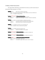
1. MODEL OVERVIEW (file: S1.ps) . . . . . . . . . . . . . . . . . . . . . . . . . . . . . . . . . . . . . . . . . . 1
1.1 Features . . . . . . . . . . . . . . . . . . . . . . . . . . . . . . . . . . . . . . . . . . . . . . . . . . . . . . . . .
1.2 Pre-Installation Preparation . . . . . . . . . . . . . . . . . . . . . . . . . . . . . . . . . . . . . . . . . .
1.3 Windows 95/98/NT Installation . . . . . . . . . . . . . . . . . . . . . . . . . . . . . . . . . . . . . . .
1.4 Quick Start . . . . . . . . . . . . . . . . . . . . . . . . . . . . . . . . . . . . . . . . . . . . . . . . . . . . . .
1.5 Problems . . . . . . . . . . . . . . . . . . . . . . . . . . . . . . . . . . . . . . . . . . . . . . . . . . . . . . . .
1
2
3
5
8
2. ADVANCED SIMULATION CONTROL (file: S2.ps) . . . . . . . . . . . . . . . . . . . . . . . . . . . 9
2.1 Trajectories . . . . . . . . . . . . . . . . . . . . . . . . . . . . . . . . . . . . . . . . . . . . . . . . . . . . . . . . 9
2.2 Air Concentration . . . . . . . . . . . . . . . . . . . . . . . . . . . . . . . . . . . . . . . . . . . . . . . . . . . 11
2.2.1 Meteorological Simulation Entries . . . . . . . . . . . . . . . . . . . . . . . . . . . . . . . .
2.2.2 Pollutant Definition Entries . . . . . . . . . . . . . . . . . . . . . . . . . . . . . . . . . . . . . .
2.2.3 Concentration Grid Definition . . . . . . . . . . . . . . . . . . . . . . . . . . . . . . . . . . . .
2.2.4 Deposition Definitions . . . . . . . . . . . . . . . . . . . . . . . . . . . . . . . . . . . . . . . . .
11
13
13
16
3. GRAPHICAL DISPLAY OPTIONS ( file: S3.ps) . . . . . . . . . . . . . . . . . . . . . . . . . . . . . . . 18
3.1 Trajectories . . . . . . . . . . . . . . . . . . . . . . . . . . . . . . . . . . . . . . . . . . . . . . . . . . . . . . . . 18
3.2 Air Concentration . . . . . . . . . . . . . . . . . . . . . . . . . . . . . . . . . . . . . . . . . . . . . . . . . . . 19
3.3 Utility Programs . . . . . . . . . . . . . . . . . . . . . . . . . . . . . . . . . . . . . . . . . . . . . . . . . . . . 20
3.3.1 Con2asc - convert to ASCII . . . . . . . . . . . . . . . . . . . . . . . . . . . . . . . . . . . . .
3.3.2 Con2stn - grid to station . . . . . . . . . . . . . . . . . . . . . . . . . . . . . . . . . . . . . . . .
3.3.3 Wincpick - select from display . . . . . . . . . . . . . . . . . . . . . . . . . . . . . . . . . . .
3.3.4 Timeplot - time series concentration plot . . . . . . . . . . . . . . . . . . . . . . . . . . . .
20
20
22
22
3.4 Output Customization . . . . . . . . . . . . . . . . . . . . . . . . . . . . . . . . . . . . . . . . . . . . . . . . 23
3.5 File Formats . . . . . . . . . . . . . . . . . . . . . . . . . . . . . . . . . . . . . . . . . . . . . . . . . . . 23
3.5.1 Trajectory Endpoints . . . . . . . . . . . . . . . . . . . . . . . . . . . . . . . . . . . . . . . . . . . 23
3.5.2 Binary Gridded Concentrations . . . . . . . . . . . . . . . . . . . . . . . . . . . . . . . . . . . 24
4. SPECIAL APPLICATIONS ( file: S4.ps) . . . . . . . . . . . . . . . . . . . . . . . . . . . . . . . . . . . . . . 25
4.1 Particle or Puff Releases . . . . . . . . . . . . . . . . . . . . . . . . . . . . . . . . . . . . . . . . . . . . . .
4.2 Continuous Emissions . . . . . . . . . . . . . . . . . . . . . . . . . . . . . . . . . . . . . . . . . . . . . . . .
4.3 Gridded Area Source Emissions . . . . . . . . . . . . . . . . . . . . . . . . . . . . . . . . . . . . . . . .
4.4 Namelist File: SETUP.CFG . . . . . . . . . . . . . . . . . . . . . . . . . . . . . . . . . . . . . . . . . . .
4.5 Compilation Limits: DEFSIZE.INC . . . . . . . . . . . . . . . . . . . . . . . . . . . . . . . . . . . . .
iii
25
25
25
26
29
4.6 Optional Features - Advanced GUI Menu . . . . . . . . . . . . . . . . . . . . . . . . . . . . . . . . .
4.7 Configuration for Operational Applications . . . . . . . . . . . . . . . . . . . . . . . . . . . . . . .
4.8 Backward Dispersion Simulations . . . . . . . . . . . . . . . . . . . . . . . . . . . . . . . . . . . . . . .
4.9 Time Variation of the Emission Rate . . . . . . . . . . . . . . . . . . . . . . . . . . . . . . . . . . . .
31
31
33
33
5. METEOROLOGICAL INPUT DATA ( file: S5.ps) . . . . . . . . . . . . . . . . . . . . . . . . . . . . . . 34
5.1 Valid Meteorological Data Types . . . . . . . . . . . . . . . . . . . . . . . . . . . . . . . . . . . . . . .
5.2 Creation of a Meteorological Input Data File . . . . . . . . . . . . . . . . . . . . . . . . . . . . . .
5.3 Decoding Meteorological Data Files . . . . . . . . . . . . . . . . . . . . . . . . . . . . . . . . . . . . .
5.4 Sample Meteorological Programs . . . . . . . . . . . . . . . . . . . . . . . . . . . . . . . . . . . . . . .
5.5 Meteorological GUI Menu Tab . . . . . . . . . . . . . . . . . . . . . . . . . . . . . . . . . . . . . . . . .
36
37
40
41
43
6. ACKNOWLEDGEMENTS (file: S6.ps) . . . . . . . . . . . . . . . . . . . . . . . . . . . . . . . . . . . . . . 46
iv
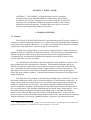
HYSPLIT_4 USER’s GUIDE
ABSTRACT. The HYSPLIT_4 (Hybrid Single-Particle Lagrangian
Integrated Trajectory) Model installation, configuration, and operating
procedures are reviewed. Examples are given for setting up the model for
trajectory and concentration simulations, graphical displays, and creating
publication quality illustrations. Programs that can be used to create the
model’s meteorological input data are described.
1. MODEL OVERVIEW
1.1 Features
The HYsplit_4 (HYbrid Single-Particle Lagrangian Integrated Trajectory) model is a
complete system for computing trajectories to complex dispersion and deposition simulations
using either puff or particle approaches. 1 It consists of a modular library structure with main
programs for each application: trajectories and air concentrations.
Gridded meteorological data, on one of three conformal (Polar, Lambert, Mercator)
map projections, are required at regular time intervals. The input data are interpolated to an
internal sub-grid to reduce memory requirements and increase computational speed.
Calculations may be performed sequentially on multiple meteorological grids, usually
specified from fine to coarse resolution.
Air concentration calculations require the definition of the pollutant’s emissions and
physical characteristics (if deposition is required). When multiple pollutant species are
defined, an emission would consist of one particle or puff associated with each pollutant
type. Alternately, the mass associated with a single puff may contain several species. The
latter approach is used for calculation of chemical transformations when all the species
follow the same transport pathway. Chemical transformation subroutines are not part of the
model distribution.
The dispersion of a pollutant is calculated by assuming either a Gaussian or Top-Hat
horizontal distribution within a puff or from the dispersal of a fixed number of particles. A
single released puff will expand until its size exceeds the meteorological grid cell spacing
and then it will split into several puffs. An alternate approach combines both puff and
particle methods by assuming a puff distribution in the horizontal and particle dispersion in
the vertical direction. The resulting calculation may be started with a single particle. As its
horizontal distribution expands beyond the grid length scale, it will split into multiple
particle-puffs, each with their respective fraction of the pollutant mass. In this way, the
greater accuracy of the vertical dispersion parameterization of the particle model is combined
with the advantage of having an expanding number of particles represent the pollutant
1
Draxler, R.R., and G.D. Hess, 1998, An overview of the Hysplit_4 modelling system for trajectories,
dispersion, and deposition, Australian Meteorological Magazine, 47, 295-308 .
1
distribution as the spatial coverage of the pollutant increases.
Air concentrations are calculated at a specific grid point for puffs and as cell-average
concentrations for particles. A concentration grid is defined by latitude-longitude
intersections. Simultaneous multiple grids with different horizontal resolutions and temporal
averaging periods can be defined for each simulation. Each pollutant species is summed
independently on each grid.
The routine meteorological data fields required for the calculations may be obtained
from existing archives or from forecast model outputs already formatted for input to Hysplit.
In addition, pre-processor programs are provided to convert NOAA, NCAR (National Center
for Atmospheric Research) re-analysis, or ECMWF (European Centre for Medium-range
Weather Forecasts) model output fields to a format compatible for direct input to the model.
The model’s meteorological data set structure is compressed and in "direct-access" format.
Each time period within the data file contains an index record that includes grid definitions to
locate the spatial domain, check-sums for each record to ensure data integrity, variable
identification, and level information. These data files require no conversion between
computing platforms.
The modeling system includes a Graphical User Interface (GUI) to set up a trajectory,
air concentration, or deposition simulation. The post-processing part of the model package
incorporates graphical programs to generate multi-color or black and white publication
quality Postscript printer graphics.
A complete description of all the equations and model calculation methods for
trajectories and air concentrations has been published,2 and is also available on-line
(http://www.arl.noaa.gov/hysplit.html).
1.2 Pre-Installation Preparation
Although the self-installing executable, hysplit4{x}.exe, does not require any
additional software, it will only provide a command line interface to the model. To enable
the model’s GUI, the computer should have Tcl/Tk script language installed. It can be
obtained over the Internet from: http://dev.scriptics.com. The installation of Tcl/Tk will
result in the association of the .tcl suffix with the Wish executable and all Hysplit GUI scripts
will then show the Tk icon.
The Hysplit GUI contains options to convert either the trajectory or concentration
model output files to Postscript. The Postscript files can also be viewed directly through the
GUI if a Postscript viewer, such as Ghostscript has been installed prior to the Hysplit
installation. See www.cs.wisc.edu/~ghost for more information on Postscript viewers.
2
Draxler, R.R., and G.D. Hess, 1997, Description of the Hysplit_4 modeling system, NOAA
Technical Memorandum ERL ARL-224, December, 24p .
2
1.3 Windows 95/98/NT Installation
Hysplit installation to a computer running Windows (16 bit versions are not
supported) is provided through a self installing file. Executables are installed in various
directories for trajectories, dispersion, display of results, manipulation of results, and creation
of input meteorological data files. The trajectory and dispersion model source code is not
provided. However all the Fortran source code to create meteorological data files in a format
that the model can read are provided in the \metdata directory. Each subdirectory contains a
Readme.txt file with more complete information about the contents of that directory.
At the beginning of the installation you will be prompted as to the directory location.
It is suggested you select the default location (C:\hysplit4). The installation program is very
simple and although the selection of a different drive or directory will install the code in the
selected directories, the shortcut links will not be placed correctly in the Start Menu or
Desktop. In this situation you will need to edit the \icons\setup.bat file for the correct drive
and directory locations.
The following subdirectories will be created after the installation has completed:
bdyfiles - This directory contains an ASCII version of gridded land use, roughness length,
and terrain data. The current file resolution is 360 x 180 at 1 degree. The upper left corner
starts at 180 W, 90 N. The files are read by both Hysplit executables, hymodelt and
hymodelc, from this directory. If not found, the model uses default constant values for
land-use and roughness length. The data structure of these files is defined in the file
ASCDATA.CFG, which should be located in either the model’s startup directory or the
\bdyfiles directory. This file defines the grid system and gives an optional directory location
for the land-use and roughness length files. These files may be replaced by higher resolution
customized user-created files. However, regardless of their resolution, the model will only
apply the data from these files at the same resolution as the input meteorological data grid.
More information on the structure of these files can be found in the local Readme.txt file.
data2arl - Current forecast or archive meteorological data can be obtained from the ARL ftp
server: ftp://gus.arlhq.noaa.gov /pub/archives (or /forecasts). Older archive data can be
ordered from the NCDC (National Climatic Data Center). However if you have access to
your own meteorological data or data formatted as GRIB (Gridded Binary), this directory
contains various example decoder programs to convert meteorological data in various
formats to the format (ARL packed) that Hysplit can read. Sample programs include GRIB
decoders for ECMWF model fields, NCAR/NCEP (National Centers for Environmental
Prection) re-analysis data, and NOAA Aviation and Regional Spectral Model files. All the
required packing and unpacking subroutines can be found in the various subdirectories of
\data2arl. More information on these programs can be found in Section 5.4.
concmdl - The directory contains the Hysplit4 air concentration prediction model ( hymodelc)
and related display programs. Although the model can be run through the GUI, at times it
may be desirable to run the model from the command line (e.g. using automated scripts).
The example Control file should produce some results for viewing. The sequence of
3
commands would be hymodelc to execute the model, and concplot to create a Postscript file
called concplot.ps. Command line arguments are required for concplot. Normally the GUI
is used to create the Control file for the simulation. If the file is missing, the model will
prompt you for input from the keyboard. Your inputs are copied to a file called Startup.
That file may then be edited and renamed to Control for subsequent simulations. Conread
and con2asc are provided as examples of how to read concentration files for users to develop
other applications.
document - This directory contains PDF (Adobe Portable Document Format) versions of the
User’s Guide and other documentation such as ARL-224, the principal ARL Technical
Memorandum describing the model and equations. This User’s Guide (this document)
provides detailed instructions in setting up the model, modifications to the Control file to
perform various simulations and output interpretation. The Readme.txt file contains
additional information about compilation, typical CPU times, and a summary of recent model
updates.
graphics - There are two types of graphical plotting programs provided in the \concmdl and
\trajmdl directories. Publication quality graphics can be created using the postscript
conversion programs, concplot and trajplot, which use a Fortran Postscript library created by
Kevin Kohler3. All graphical routines use the map background file arlmap in this directory.
The map background file uses a simple ASCII format and contains the world’s coastal and
political boundaries at relatively coarse resolution. Other higher resolution map background
files are available from the Hysplit download web page. All graphical programs search the
startup directory first for arlmap before going to \graphics, therefore customized maps can
be created without changing the Hysplit installation structure.
guicode - This directory contains a Tcl/Tk GUI interface source code script for Hysplit. The
interface is used to set up the input Control file as well as run the graphical output display
programs. To use the interface you must first install Tcl/Tk. The upper-level Tcl script is
called hysplit4.tcl, which calls all other Tcl scripts. The Hysplit GUI is started by executing
this script. The Desktop short-cut as well as the Start Menu options should point to this
script. If the installation program did not properly setup the Desktop, you should copy the
shortcut from \working or you can manually create a short-cut to the script and edit its
properties such that the "Start In" directory is \working. You should also select the Hysplit
icon from the \icons directory before moving it to the Desktop.
icons - Normally if you install Hysplit to the default drive c:\hysplit4, there should be a
desktop icon as well as entries in the Start Programs menu. If these short-cuts were not set
up properly, you can edit the Setup.bat file to reflect your directory structure. If you still
have trouble, then the icons supplied in this directory can be used to replace the default
Windows icons if you create shortcuts to Hysplit from the desktop. Use the right mouse
button and select: Properties | Shortcut | Change Icon. Note that the \working\hysplit4.tcl
shortcut should be copied to the desktop.
3
PSPLOT libraries can be found at www.nova.edu/ocean/psplot.html and were created by Kevin
Kohler ([email protected]).
4
metdata - This directory contains the sample meteorological data file: oct1618.BIN. It is an
extract of the NGM (NOAA’s Nested Grid Model) over the US from 0000 UTC 10/16/95
through 0000 UTC of 10/18/95. The file is used for all calculations shown in the User's
Guide. In addition, several sample programs are provided that can be used to examine and
display the meteorological data files. Source code for some of these routines can be found in
the \source subdirectory. More information on these programs can be found in Section 5.4.
trajmdl - This directory contains the Hysplit4 trajectory model (hymodelt) and related
display programs. Although the model can be run through the GUI, at times it may be
desirable to run the model from the command line (e.g. automated scripts). The example
Control file should produce some results for viewing. The sequence of commands would be
hymodelt to execute the model, and trajplot to create a Postscript file called trajplot.ps.
Normally the GUI is used to create the Control file for the simulation. If the file is missing,
the model will prompt you for input from the keyboard. Your inputs are copied to a file
called Startup. That file may then be edited and renamed to Control for subsequent
simulations.
visualization - contains Fortran source code and some executables to convert trajectory, air
concentration, and meteorological data files for input to GRADS and VIS5D.
working - This should be the default working directory when running the model through the
GUI. The properties of the Hysplit4 shortcut should point to this as the startup directory.
This directory will contain all the user created input and output files unless they are explicitly
directed to be read or written from/to another directory in the input Control file, such as
meteorological data files that might be found in \metdata. A sample tcl script, Auto_traj.tcl,
is provided as an example of how one might automate multiple trajectory calculations. The
script creates the Control file and executes the model in a loop, varying specific parameters
with each simulation.
1.4 Quick Start
The easiest way to run the model is to use the GUI menu to edit the model's input
Control file. For the purposes of this demonstration appropriate meteorological files are
provided. If for some reason the menu system is not available, the Control file can be
created manually. See the discussion in Section 2.
Step 1 - start the GUI menu system using \working\hysplit4.tcl or the desktop shortcut to
Hysplit4. A widget will appear with the HYSPLIT graphic and two button options: Menu
and Exit. On some systems the graphic may be scrambled or the colors may be flat.
Switching the PC display to VGA and 256 colors usually solves these problems. However it
can be left alone as the faulty graphic will not affect any of the other widgets or display
graphics.
Step 2 - from the HYSPLIT graphic widget click on Menu. The three main menus of
Hysplit4 will appear: Meteorology, Trajectory, Concentration, and on some custom
installations the optional menu: Advanced. An additional small widget underneath the main
menu gives the current Hysplit4 version information. Do not delete this widget as it will
5
terminate the GUI. It provides the reference frame for the model’s standard output and
messages.
Step 3 - for the first example calculation select the Trajectory option. Four options appear
under this item: Trajectory Setup, Run Model, Trajectory Display, and Utility Programs.
Normally these are run in sequence, however any item can be selected and run if the
appropriate input files were created during a previous simulation. Currently no utility
program options are available.
Step 4 - Trajectory Setup is used to enter the basic model simulation parameters: the starting
time of the calculation; starting location in terms of latitude, longitude, and height; the runtime or duration of the trajectory calculation; and the names and locations of all required
files. When modifications to this menu are complete, click on Save. However for this
example, you will use the Retrieve option for predefined configurations, so do nothing here
and go on to Step 5.
Step 5 - for the sample calculation click on Retrieve, enter name of the example preconfigured control file: sample_traj, then click on OK, then after the data entry widget is
closed, click on Save and the setup menu will close.
Step 6 - Run Model copies the setup configuration to the model's input Control file and starts
the model calculation. Messages will appear on standard output showing the progress of the
calculation. When the simulation is completed, the trajectory end-points output file is ready
to be converted to a graphical display. Under Windows 95/98 the standard output widget
will not show any output until the end of the calculation and the Trajectory menu items will
be locked until the calculation completes.
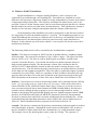
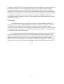
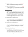
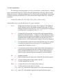
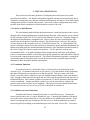
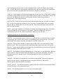
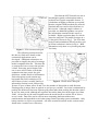
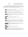
Step 7 - selecting Display will run a
special program that converts the
ASCII file of trajectory end-point
positions into a high quality Postscript
file (trajplot.ps) suitable for printing.
The conversion widget provides
options for the frequency of the labels
on the trajectory, a "HiResolution"
(zoomed) display, and color or black
and white graphics. If a Postscript
viewer (Ghostscript / Ghostview) has
been installed and associated with the
.ps file suffix, then it will be invoked
by the GUI. If the viewer does not
automatically open, it may be
necessary to manually edit hysplit4.tcl
to change the directory location
associated with the program
gsview32.exe. The sample output from
the Postscript file is shown in Fig. 1.
Figure 1. Example from Postscript conversion.
6
In the example case, trajectory positions are marked at 6-h intervals and the vertical
projection is shown in the lower panel with each point below its corresponding point on the
horizontal projection..
Step 8 - for the second example calculation select Concentration. Under this menu there are
also four options: concentration setup, run model, concentration display, and Utility
Programs. In general they should be executed in sequential order.
Step 9 - selecting Concentration Setup brings up similar starting information as with
trajectories, but with three additional sub-menus (Pollutant) that can be used set the emission
rate, duration, and start time of the emission; ( Grids) to set the location, resolution, levels,
and averaging times of the concentration output grid; and (Deposition) to set the
characteristics of each pollutant. Click on Retrieve, enter name of sample pre-configured
control file: sample_conc, then click on OK, then after the data entry widget is closed, click
on Save and the setup menu will close.
Step 10 - selecting Run Model copies the setup configuration to the model’s input Control file
and starts the model calculation. Messages will appear on standard output showing the
progress of the calculation after the calculation has completed. At that point the binary
gridded concentration output file is ready to be converted to a graphical display. Be patient
as concentration calculations may take considerably longer than trajectory calculations.
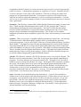
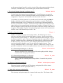
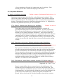
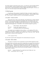
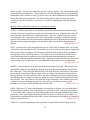
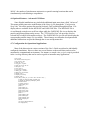
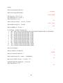
Step 11 - selecting Display will run a
special program that converts the
binary concentration file to a
Postscript file (concplot.ps) suitable
for printing. The display widget
contains multiple options for different
pollutants (if defined), data grids,
levels, and contour options. These
are discussed in more detail in the
"Graphics" section. For this example
accept the defaults and just click on
"Execute Display." If the Ghostview
Postscript viewer has been installed
and properly associated with .ps files,
then it will be automatically invoked
by the GUI. If the viewer does not
open, it may be necessary to manually
edit the file hysplit4.tcl for the
directory entry associated with the
Figure 2. Example from the Postscript conversion.
program gsview32.exe. The sample
output from the Postscript file is
shown in Fig. 2. The output file can be printed directly on any Postscript printer or printed
through Ghostscript.
Step 12 - selecting Utility Programs brings up options for three different utility programs:
7
"Convert to ASCII" which will run a program that converts the binary air concentration file to
an ASCII file with one record for each non-zero grid point giving the latitude-longitude
position and air concentration. The file can be used as input to GIS or other visualization
programs; "Grid to Station" will extract a concentration time series at one or more locations
to an output text file; and "Select from Display" shows a coarse graphic screen display of the
concentration field and uses the mouse to selection of points at which the position and
concentration value is written to a text file. These programs will be discussed in more detail
in the graphics section.
1.5 Problems
If Tcl/Tk does not exist on your system or there are other problems with the GUI
interface, it is very easy to run the sample cases directly in either the \trajmdl or \concmdl
sub-directories by double-clicking on hymodelt, trajplot for trajectories and hymodelc,
concplot for air concentrations. If the sample simulation works well, then it is only necessary
to manually edit the Control file to try out different simulation variations. The other options
are explained in more detail in Section 2.
In general, premature termination during the model initialization phase will result in
messages to standard output. However after the model has started, fatal, diagnostic, and
progress notification messages are written to a file called Message. If the model output is not
what you expected, first check the Control file to determine if the input setup is what is
desired, then check the Message file for indication of abnormal performance. These files are
always written to the model’s startup directory % \working if the model is run from the GUI.
8
2. ADVANCED SIMULATION CONTROL
When the model starts it looks for an input file called Control. If found, this file is
used to read all input parameters. If not found, a prompt will appear on standard input
requesting appropriate information. These prompts are described in more detail below and
are identical to the comparable entries through the GUI menu. When data entry is through
the keyboard, a file named Startup is created. This contains a copy of the input, and which
later may be renamed to Control to permit direct editing and model execution without data
entry. If you are unsure as to a value required in an input field, just enter the forward slash
(/) character, the indicated default value will be used. This default procedure is valid for all
input fields except directory and file names. An automatic default selection procedure is also
available when the input fields are read from the Control file for certain fields when they are
set to zero. Those options are discussed in more detail below. Each input line is numbered
(only in this text) according to the order it appears in the file. A number in parenthesis after
the line number indicates that there is an input loop and multiple entry lines may be required
depending upon the value of the previous entry.
2.1 Trajectories
1- Enter starting time (year, month, day, hour)
Default: 0 0 0 0
Enter the two digit values for the UTC time that the calculation is to start. Use 0’s to
start at the beginning (or end) of the file according to the direction of the calculation.
Zero’s will force the calculation to use the time of the first (or last) record of the
meteorological data file.
2- Enter number of starting locations
Default: 1
Simultaneous trajectories can be calculated at multiple levels or starting locations.
The maximum number depends upon the compilation parameters. The GUI
menu can accommodate up to 6 simultaneous starting locations. Specification of
additional locations requires manual editing of the Control file.
3(1)- Enter starting location (lat, lon, meters)
Default: 40.0 -90.0 50.0
Position in degrees and decimal (West and South are negative). Height is
entered as meters above ground. See section 4.4 on how to set heights relative
to mean sea level.
4- Enter total run time (hours)
Default: 48
Specify the duration of the calculation in hours. Backward calculations are entered as
negative hours.
5- Vertical motion option (0:data 1:isob 2:isen 3:dens 4:sigma)
Default: 0
Indicates the vertical motion calculation method. The default "data" selection will
9
use the meteorological model’s vertical velocity fields; other options include isobaric,
isentropic, constant density, and constant sigma (internal model coordinate).
6- Top of model domain (internal coordinates m-agl)
Default: 10000.0
Vertical limit of the internal meteorological grid. If calculations are not required
above a certain level, fewer meteorological data are processed thus speeding up the
computation. Trajectories will terminate when they reach this level.
A secondary use of this parameter is to set the model’s internal scaling height % the
height at which the internal sigma surfaces go flat relative to terrain. The default
internal scaling height is set to 25 km but it is set to the top of the model domain if
the entry exceeds 25 km. Further, when meteorological data are provided on terrain
sigma surfaces it is assumed that the input data were scaled to a height of 20 km. If a
different height is required to decode the input data it should be entered on this line as
a negative of the height. Hysplit’s internal scaling height remains at 25 km unless the
absolute value of the domain top exceeds 25 km.
7- Number of input data grids
Default: 1
Number of simultaneous input meteorological files. The following two entries
(directory and name) will be repeated this number of times. Always start with the
finest resolution grid as number #1. When the computation shifts from grid #1 to #2,
it will not return to #1 again. The run will terminate when the computation is off the
last grid. Multiple trajectory calculations will switch grids for all trajectories when
the first trajectory passes to the new grid. Multiple grid definitions also have the
restriction that there should be some overlap between the grids in space. Time
overlap, although desirable, is not required. However, without time overlap it is not
possible to interpolate in time across grids and hence start trajectories at those times.
8(1)- Meteorological data grid # 1 directory
Default: \main\sub\data\
Directory location of the meteorological file on the grid specified. Always
terminate with the appropriate slash (\).
9(2)- Meteorological data grid # 1 file name
Default: file_name
Name of the file containing meteorological data. Located in the previous
directory.
10- Directory of trajectory output file
Default: \main\trajectory\output\
Directory location to which the ASCII trajectory end-points file will be written.
Always terminate with the appropriate slash (\).
11- Name of the trajectory endpoints file
Default: file_name
The trajectory end-points output file is named in this entry line. The format of the
10
file is given in Section 6.
2.2 Air Concentration
The entries in the Control file for air concentration simulations consist of four groups
of input data. The first group is almost identical to the trajectory simulation. The second
group defines the pollutant emission characteristics. The third group defines the
concentration grid in terms of spacing and integration interval. The fourth group of entries
defines pollutant characteristics relevant to computing deposition and removal processes.
2.2.1 Meteorological Simulation Entries
1- Enter starting time (year, month, day, hour)
Default: 0 0 0 0
Enter the two digit values for the UTC time that the calculation is to start. Use 0’s to
start at the beginning of the file. Note that the calculation start time may be different
from the emission start time that is specified below. However the simulation start
time may not occur after the emission start time.
2- Number of starting locations
Default: 1
Multiple pollutant sources may be simultaneously tracked. The emission rate
specified below is assigned to each source. In addition, the emissions are distributed
vertically in a layer between the current emission height and the previous source
emission height if the previous source is at the same location. The effective source
will be a vertical line source between the two heights. When multiple sources are in
different locations, the pollutant is emitted as a point source from each location at the
height specified. Point and vertical line sources can be mixed in the same simulation.
The GUI menu can accommodate up to 6 simultaneous starting locations.
Specification of additional locations requires manual editing of the Control file. Area
source emissions can be specified from an input file: emission.txt. When this file is
present in the root directory, the emission parameters in the Control file are
superceded by the emission rates specified in the file. More information on this file
structure can be found in Section 4.2.
3(1)- Enter starting location (lat, lon, meters, Opt-4, Opt-5) Default: 40.0 -90.0 50.0
Position in degrees and decimal (West and South are negative). Height is
entered as meters above ground level unless the mean-sea-level flag has been
set (see section 4.4).
The optional 4th (emission rate - units per hour) and 5 th (emission area - square
meters) columns on this input line can be used to supercede the value of the
emission rate (line 12-2) when multiple sources are defined, otherwise all
sources have the same rate as specified on line 12-2. The 5 th column defines
the virtual size of the source: point sources default to "0".
11
4- Enter total run time (hours)
Default: 48
The duration of the calculation in hours. Backward calculations are indicated by a
negative run time. See discussion in Section 4 on backward "dispersion" calculations.
5- Vertical (0:data 1:isob 2:isen 3:dens 4:sigma)
Default: 0
Indicates the vertical motion calculation method. The default "data" option uses the
meteorological model’s vertical velocity fields; other options include isobaric,
isentropic, constant density, and constant sigma above terrain.
6- Top of model domain (internal coordinates m AGL)
Default: 10000.0
Vertical limit of the internal grid. If calculations are not required above a certain
level, fewer meteorological data are processed, thus speeding up the computation.
Particles and puffs are restricted from mixing above this level. Complete reflection is
assumed.
A secondary use of this parameter is to set the model’s internal scaling height % the
height at which the internal sigma surfaces go flat relative to terrain. The default
internal scaling height is set to 25 km but it is set to the top of the model domain if
the entry exceeds 25 km. Further, when meteorological data are provided on terrain
sigma surfaces it is assumed that the input data were scaled to a height of 20 km. If a
different height is required to decode the input data it should be entered on this line as
a negative of the height. Hysplit’s internal scaling height remains at 25 km unless the
absolute value of the domain top exceeds 25 km.
7- Number of input data grids
Default: 1
Number of simultaneous meteorological fields to be input. The following two entries
(directory and name) will be repeated this number of times. Always start with the
finest resolution grid as number #1. When the first puff or particle moves on to the
next grid, all subsequent particles are automatically transferred to the new grid.
There should be time and space overlap for multiple grids.
Default: \main\sub\data\
8(1)- Enter grid # 1 directory
Directory location of the meteorological files. Terminate with appropriate (\)
slash.
9(2)- Enter grid # 1 file name
Default: file_name
Name of the meteorological data file.
12
2.2.2 Pollutant Definition Entries
10- Number of different pollutants
Default: 1
Multiple pollutant species may be defined for emission. Each pollutant is assigned to
its own particle or puff and therefore may behave differently due to deposition or
other pollutant specific characteristics. Each will be tracked on its own concentration
grid. The following four entries are repeated for each pollutant defined. Although
the GUI shows that up to seven pollutants can be defined, the compilation default is
to permit only two simultaneous definitions.
11(1)- Pollutant four Character Identification
Default: TEST
Any four-character label that can be used to identify the pollutant. The label
is written with the concentration output grid to identify output records
associated with that pollutant and will appear in display labels. Additional
user supplied deposition and chemistry calculations may be keyed to this
identification string.
Default: 1.0
12(2)- Emission rate (per hour)
Mass units released each hour. Units are arbitrary except when specific
chemical transformation subroutines are associated with the calculation.
Output air concentration units will be in the same units as specified on this
line: input kg/hr -> output kg/m 3; input Bq/hr -> output Bq/m 3. When
multiple sources are defined this rate is assigned to all sources unless optional
parameters are present on line 3(1).
13(3)- Hours of emission
Default: 1.0
The duration of emission may be defined in fractional hours. Durations of
less than one time-step will be emitted over one time-step with a total
emission that would yield the requested rate over the emission duration.
"Backward" simulations require a negative value for the hours of emission.
14(4)- Release start time: year month day hour minute
Default: [simulation start time]
The previously specified hours of emission start at this time. An entry of
zero’s in the field, when input is read from a file, will also result in the
selection of the default values. "Backward" calculations require this field to
be set with explicit rather than relative or default values.
2.2.3 Concentration Grid Definition
Dispersion calculations are performed on the computational (meteorological) grid
without regard to the definition or location of any concentration grid. Therefore it is possible
to complete a simulation and have no results to view if the concentration grid was in the
13
wrong location. In addition, the concentration grid spacing may restrict the model’s
integration time step to a smaller value for higher resolution concentration grids. This
section is used to define the grid system to which the concentrations are summed during the
integration and subsequently for postprocessing and display of the model’s output.
15- Number of simultaneous concentration grids
Default: 1
Multiple or nested grids may be defined. The concentration output grids are treated
independently. The following 10 entries will be repeated for each grid defined. The
number of grids permitted depends upon model compilation parameters % the default
compilation is usually supports two independent grids.
16(1)- Center Latitude, Longitude (degrees)
Default: [source location]
The center position of the concentration sampling grid in degrees and decimal.
Input of zero’s will result in selection of the default value: location of the
emission source. Sometimes it may be desirable to move the grid center
location downwind near the center of the projected plume position.
17(2)- Grid spacing (degrees) Latitude, Longitude
Default: 1.0 1.0
The interval in degrees between nodes of the sampling grid. Puffs must pass
over a node to contribute concentration to that point and therefore if the
spacing is too wide, they may pass between intersection points. Particle
model calculations represent grid-cell averages, where each cell is centered on
a node position, with its dimensions equal to the grid spacing. Finer
resolution concentration grids require correspondingly finer integration timesteps. This may be mitigated to some extent by limiting fine resolution grids
to only the first few hours of the simulation.
18(3)- Grid span (deg) Latitude, Longitude Default: [max-Y / d-lat] [max-X / d-lon]
The total span of the grid in each direction. For instance, a span of 10 degrees
would cover 5 degrees on each side of the center grid location. A default span
is computed from the compiled maximum dimensions of the concentration
grid divided by the grid spacing requested in the previous entry. The typical
default compilation size supports a 300x300 node grid. If a grid resolution of
0.1 deg (about 10 km) was selected, then the maximum grid span would be 30
degrees latitude-longitude. A plume that goes off the grid would have cutoff
appearance. This can sometimes be mitigated by moving the grid center
further downwind.
Default: \main\sub\output\
19(4)- Enter grid # 1 directory
Directory to which the binary gridded concentration output file for this grid is
written. As in other directory entries a terminating (\) slash is required.
14
20(5)- Enter grid # 1 file name
Default: file_name
Name of the concentration output file for each grid. See Section 6 for a
description of the format of the concentration output file.
21(6)- Number of vertical concentration levels
Default: 1
The number of vertical levels in the concentration grid including the ground
surface level if deposition output is required. The default compilation usually
supports up to 10 levels.
22(7)- Height of each level (m)
Default: 50
Output grid levels may be defined in any order for the puff model as long as
the deposition level (0) comes first (a height of zero indicates deposition
output). Air concentrations must have a non-zero height defined. A height
for the puff model indicates the concentration at that level. A height for the
particle model indicates the average concentration between that level and the
previous level (or the ground for the first level). Therefore heights for the
particle model need to be defined in ascending order. Note that the default is
to treat the levels as above-ground-level (AGL) unless the the MSL (above
Mean-Sea-Level) flag has been set (see Section 4.4).
23(8)- Sampling start time: year month day hour minute
Default: [simulation start time]
Each concentration grid may have a different starting, stopping, and output
averaging time. Zero entry will result in setting the default values.
"Backward" calculations require this and the following parameter to be
explicitly set and further the stop time should come before the start time.
24(9)- Sampling stop time: year month day hour minute
Default: {+1} 12 31 24 60
After this time no more concentration records are written. Early termination
of high resolution grids (after the plume has moved away from the source) is
an effective way of speeding up the computation for high resolution output
because that particular grid resolution is no longer used for time-step
computations.
25(10)- Sampling interval: type hour minute
Default: 0 24 0
Each grid may have its own sampling or averaging interval. The interval can
be of two different types: averaging (type=0) or snapshot (type=1).
Averaging will produce output averaged over the specified interval. Snapshot
will give the instantaneous output at the output interval. For instance you may
want to define a concentration grid that produces 24-hour average air
concentrations for the duration of the simulation which for the default case of
15
a 2-day simulation will result in 2 output maps, one for each day. Each
defined grid can have a different output type and interval.
2.2.4 Deposition Definitions
26- Number of pollutants depositing
Default: number of pollutants defined on line # 10
Deposition parameters must be defined for each pollutant species emitted. Each
species may behave differently for deposition calculations. Each will be tracked on
its own concentration grid. The following five lines are repeated for each pollutant
defined. The number here must be identical to the number on line 10. Deposition is
turned off for pollutants by an entry of zero in all fields.
27(1)- Particle: Diameter (µm), Density (g/cc), and Shape
Default: 0.0 0.0 0.0
These three entries are used to define the pollutant as a particle for
gravitational settling and wet removal calculations. A value of zero in any
field will cause the pollutant to be treated as a gas. All three fields must be
defined (>0) for particle deposition calculations. These values need to be
correct only if gravitational settling is to be computed by the model, otherwise
a nominal value of 1.0 may be assigned as a default for each entry to define
the pollutant as a particle. If a dry deposition velocity is specified as the first
entry in the next line (28), then that value is also used as the particle settling
velocity.
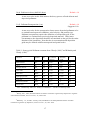
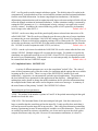
28(2)- Deposition velocity (m/s), Pollutant molecular weight (Gram/Mole),
Surface Reactivity Ratio, Diffusivity Ratio, Effective Henry’s Constant
Default: 0.0 0.0 0.0 0.0 0.0
Dry deposition calculations are performed in the lowest model layer based
upon the relation that the deposition flux equals the velocity times the groundlevel air concentration. This calculation is available for gases and particles.
The dry deposition velocity can be set directly for each pollutant by entering a
non-zero value in the first field or it can be calculated by the model using the
resistance method which requires setting the remaining four parameters
(molecular weight, surface reactivity, diffusivity, and the effective Henry’s
constant) - see Table I for more information.
29(3)- Wet Removal: Actual Henry's constant, In-cloud (L/L), Below-cloud (1/s)
Default: 0.0 0.0 0.0
Suggested: 0.0 3.2x10 5 5x10-5
Henry's constant defines the wet removal process for soluble gases. It is
defined only as a first-order process by a non-zero value in the field. Wet
removal of particles is defined by non-zero values for the in-cloud and belowcloud parameters. In-cloud removal is defined as a ratio of the pollutant in air
(g/liter of air in the cloud layer) to that in rain (g/liter) measured at the
ground. Below-cloud removal is defined through a removal time constant.
16
30(4)- Radioactive decay half-life (days)
Default: 0.0
A non-zero value in this field initiates the decay process of both airborne and
deposited pollutants.
31(5)- Pollutant Resuspension (1/m)
Default: 0.0
Suggested :10-6
A non-zero value for the resuspension factor causes deposited pollutants to be
re-emitted based upon soil conditions, wind velocity, and particle type.
Pollutant resuspension requires the definition of a deposition grid, as the
pollutant is re-emitted from previously deposited material. Under most
circumstances, the deposition should be accumulated on the grid for the entire
duration of the simulation. Note that the air concentration and deposition
grids may be defined at different temporal and spatial scales.
Table I. Some typical Pollutant constants from Wesely (1989)1 and Walmsley and
Wesely (1996)2.
Chemical
Symbol
Dhx
H* (M/atm)
effective
H(M/atm)
actual
fo
Sulfur dioxide
SO2
1.9
1x105
1.24
0.0
Ozone
O3
1.6
0.01
0.013
1.0
Nitrogen dioxide
NO2
1.6
0.01
0.01
0.1
Nitic oxide
NO
1.3
3x10-3
1.9x10-3
0.0
Nitric acid
HNO3
1.9
1x1014
2.1x105
0.0
Hydrogen peroxide
H 2O 2
1.4
1x105
1.0x105
1.0
Ammonia
NH3
0.97
2x1014
62
0.0
Peroxyacetyl nitrate
PAN
2.6
3.6
5
0.1
Nitrous acid
HNO2
1.6
1x105
2.1x105
0
Dhx - Diffusivity ratio; H - Henry’s constant; f o - Surface reactivity ratio
1
Wesely, M.L., 1989, Parameterizations of surface resistances to gaseous dry deposition in regionalscale numerical models, Atmos. Environ., 23, 1293-1304.
2
Walmsley, J. L., and M.L. Wesely, 1996, Modification of coded parameterizations of surface
resistances to gaseous dry deposition, Atmos. Environ., 30, 1181-1188.
17
18
3. GRAPHICAL DISPLAY OPTIONS
The trajectory and concentration models each generate their own output files, which are
read by the other programs to produce various displays and other output. The trajectory model
generates an ASCII file of end-point positions while the concentration model produces a binary
output file (big-endian) on a regular latitude-longitude grid. All mapping programs use the same
ASCII map background file, arlmap, which normally would be located in the \graphics
directory. However all the graphics programs search the local start directory first, then the
\graphics directory. Customized map background files could be placed in the local directory for
specialized applications. Some higher resolution map background files are available from the
Hysplit download web page. The Readme.txt file in the \graphics directory has more
information about developing custom map background files.
The feature rich Postscript conversion programs can both be accessed through the GUI or
run directly from the command line. The Postscript conversion programs for both trajectories
and concentrations have a variety of command line options, most of which are also available
through the GUI.
3.1 Trajectories
The Postscript conversion program (trajplot), found in the \trajmdl directory, reads the
trajectory endpoints output file, calculates the most optimum map for display, and creates the
output file - trajplot.ps. When executed from the command line, there are three other optional
{} inputs:
trajplot [file_name] {Size} {Color} {Labels},
where default values are in red and only the file_name is required:
Size
=0
=1
for standard resolution maps
for high resolution maps (zoomed)
Color = 0
=1
for black and white output
for color differentiation of multiple trajectories
Label = 0
=6
=12
= {X}
for no labels along the trajectory
for labels every 6 hours
for labels every 12 hours
any hour selection permitted.
The output example was shown previously in Fig. 1.
18
3.2 Air Concentration
The Postscript conversion program (concplot), found in the \concmdl directory, reads the
binary concentration output file, calculates the most optimum map for display, and creates the
output file concplot.ps. Multiple pollutant species or levels can be accommodated. Most routine
variations can be invoked from the GUI or the command line using the following 7 optional {}
parameters:
concplot [file_name] {Z1} {Z2} {Type} {Size} {Color} {Value} {Units}.
where default values are in red and only the file_name is required:
Z1, Z2
Type
Size
Heights that represent the levels that will be displayed. The heights are
always defined as meters and should correspond to the range of values
defined in the input section (line 22). The level information is interpreted
according to the Type definition. Also Z2 >= Z1.
=1
All output levels between the levels specified on the command line are
displayed as individual frames. A single level will be displayed if either
both specified levels equal the calculation level or they bracket that level.
Deposition plots are produced if available in the file and when a level
height is set to 0. If level information is omitted, all levels are displayed.
=2
The concentrations at all levels between the specified range are averaged
to produce one output frame per time period. If a deposition plot is
required then Z1 should be set to 0.
=3
A customized exposure output in which all the output concentrations are
converted to time-integrated units and vertically averaged for all levels
that are found in the file between Z1 to Z2. The last frame displayed
represents the accumulated deposition through the model simulation.
=0
=1
Standard resolution
High resolution map (less white space around the concentration pattern)
Color = 0
=1
Uses grey shade patterns for the contour color fill
Uses the standard four color fill.
Value = 0
Contour intervals are to be optimized for each map
=1
Contour intervals are the same for all maps
={X} where {X} represents the integer power of 10 of the maximum contour.
Units ={X} where {X} is the multiplier applied to the input data before output.
19
The output example was shown previously in Fig. 2. One final note is that if multiple pollutant
species are defined, a prompt to standard output will appear, requesting the selection of a
specific species. Only one pollutant species may be displayed per plot sequence. However, an
entry of "0" will cause all species to be summed for display.
3.3 Utility Programs
Currently only utility programs to manipulate the binary concentration output files are
available. Each of these programs is discussed in more detail below. All are available through
the "Utility Programs" selection of the GUI as well as through the command line.
3.3.1 con2asc - Convert to ASCII
This program can be used to convert the binary concentration file to a simple ASCII file
composed of one record per grid point for all grid points where concentrations at any level are
non-zero. Concentrations for multiple levels and pollutant species are all listed on the same
record for each grid point. The primary purpose of the conversion is to create a file that can be
imported into other applications. The format of each record in the output file is given by:
2I3
F7.2, F8.2
45E9.2
- End of Sample: Julian Day and Hour
- Latitude and Longitude of grid cell
- Concentration data (by level and pollutant)
Each output record is identified by the day (Julian: 1 to 365) and hour (UTC) of the
ending time of each sample. In addition, a new output file is created for each sampling period,
where the name of the file is composed of the {input file name}_{Julian day}_{hour}. Only the
input file name is required on the command line.
con2asc [input file name]
The selection of input file names through the GUI is determined by the Setup menu.
3.3.2 con2stn - Grid to Station
The purpose of con2stn is to list concentrations at specific latitude-longitude locations.
The program can be run from the command line, through interactive prompts from the keyboard,
or through the GUI. Command line argument syntax is that there should be no space between
the switch and options. No options are available with interactive mode. The output gives the
Julian day, month, day, and hour of the sample start; day and hour of sample ending time, and
the concentrations for each station (location selected by latitude-longitude). The format of each
output record is as follows:
F8.3,6I4
- Starting: Julian day, Year, month, day, hour; Ending: day, hour
XF10 - Concentration value at X stations
20
Unlike the other programs, the command line arguments can appear in any order and the syntax
is as follows:
con2stn -i -o -c -s -x -z -p
where the default value is indicated in red:
-i[input concentration file name: std input]
-o[output concentration file name: std output]
-c[input to output concentration multiplier: 1.0]
-s[station list file name: std input]
-x[n(neighbor) or i(interpolation): n]
-z[level index: 1]
-p[pollutant index: 1]
Unspecified file names will result in a standard input prompt. The default interpolation method
(-xn) is to used the value at nearest grid point to each latitude-longitude position. The station
positions can be read from a file (space delimited) with the first field being an integer that
represents the location identification, followed by that locations latitude and longitude.
Examples:
0) con2stn ... Results in prompts -->
Enter input concentration file name...
[name of hysplit output file]
Enter sampler ID#, latitude, longitude ...
[integer sample ID, real latitude, real longitude]
000
(to terminate input)
1) Read the model output file ’cdump’ and write text output to
file ’clist.txt’ for station #517 at 53N 85W.
con2stn -icdump -oclist.txt
517 53.0 -85.0
000
2) As in 1) but multiply all concentrations by 1000.0
con2stn -icdump -oclist.txt -c1000.0
517 53.0 -85.0
000
21
3) As in 1) but linear interpolate concentration to station rather than using the nearest grid point
con2stn -icdump -oclist.txt -xi
517 53.0 -85.0
000
4) As in 1) but read the station lat-lon from a file "slist.txt"
con2stn -icdump -oclist.txt -sslist.txt
The format of "slist.txt" is "free form", for example ...
401 39.0 -88.5
422 36.5 -87.5
657 36.0 -88.0
004 35.0 -89.0
3.3.3 wincpick - Select from Display
Windows based concentration plot point registration program is designed to read the
binary concentration data file, display the data on the screen, and then use the mouse to select
locations at which the position and concentration data are read and written to the text file:
wincpick.txt. The concentration data are displayed over the entire grid domain. If you
want to zoom in on a specific area, then it is necessary to rerun the model with a smaller
concentration grid domain. The program is available from the GUI or the command line with the
following syntax:
wincpick [input file name]
Upon startup Wincpick will display the domain background map with a summary of the mouse
based instructions: left-click registers the lat-lon position of that point to the output file
wincpick.txt. A right-click of the mouse redraws the map for the next time period and at the end
of the input file saves and closes all files; and a CNTL+right-click closes all files and exits the
program before the end of the input file. Right-click the mouse to go to the first concentration
map. Maps are drawn in sequence of height, pollutant species, and time. Left-clicks register the
lat-lon position of the mouse to the output file. If you are interested in only one time period,
skip past those times (right-click), and then register the points of interest, then CNTL-right to
exit.
3.3.4 Timeplot - Time Series Concentration Plot
timeplot -i -n
-i[input concentration file name in format as output from con2stn]
-n[sequential station number; repeat for multiple sites; 999 for all]
22
3.4 Output Customization
Many of the Postscript graphics programs that have extensive label information can be
customized to some extent, primarily the title field (upper center) and the units. This is
accomplished by placing a file called Labels.cfg in the \working or startup directory which
contains the following two entries (all in single quotes terminated by &) replacing the new string
with the desired text. A sample file called Labels.bak may be found in the relevant directory.
’TITLE&’,’NEW TITLE STRING&’
’UNITS&’,’NEW UNITS STRING&’
3.5 File Formats
3.5.1 Trajectory Endpoints
The format of the ASCII endpoints file written by the trajectory model ( hymodelt) and
read by all trajectory display programs is given below:
Record #1
I6
- Number of meteorological grids used in calculation
Records Loop #2 through the number of grids
A8
- Meteorological Model identification
5I6
- Data file starting Year, Month, Day, Hour, Forecast Hour
Record #3
I6
A8
A8
- number of different trajectories in file
- direction of trajectory calculation (FORWARD, BACKWARD)
- vertical motion calculation method (OMEGA, THETA, ...)
Record Loop #4 through the number of different trajectories in file
4I6
- starting year, month, day, hour
2F8.3 - starting latitude, longitude
F8.3
- starting level above ground (meters)
Record #5
I6
nA8
- number (n) of diagnostic output variables
- label identification of each variable (PRESSURE, THETA, ...)
Record Loop #6 through the number of hours in the simulation
I6
- trajectory number
I6
- meteorological grid number
5I6
- time of point: year month day hour minute
I6
- forecast hour at point
F8.1
- age of the trajectory in hours
2F8.3 - position latitude and longitude
F8.1
- position height in meters above ground
nF8.1 - n diagnostic output variables (1 st output always pressure)
23
3.5.2 Binary Gridded Concentrations
The output format of the binary concentration file written by hymodelc and read by all
concentration display programs is as follows:
Record #1
CHAR*4
Meteorological MODEL Identification
INT*4 Meteorological file starting time ( YEAR, MONTH, DAY, HOUR, FORECAST)
INT*4 NUMBER of starting locations
Record #2 Loop to record: Number of starting locations
INT*4 Release starting time ( YEAR, MONTH, DAY, HOUR)
REAL*4
Starting location and height ( LATITUDE, LONGITUDE, METERS)
Record #3
INT*4 Number of (LATITUDE-POINTS, LONGITUDE-POINTS)
REAL*4
Grid spacing (DELTA-LATITUDE, DELTA-LONGITUDE)
REAL*4
Grid lower left corner (LATITUDE, LONGITUDE)
Record #4
INT*4 NUMBER of vertical levels in concentration grid
INT*4 HEIGHT of each level (meters above ground)
Record #5
INT*4 NUMBER of different pollutants in grid
CHAR*4
Identification STRING for each pollutant
Record #6 Loop to record: Number of output times
INT*4 Sample start (YEAR MONTH DAY HOUR MINUTE FORECAST)
Record #7 Loop to record: Number of output times
INT*4 Sample stop (YEAR MONTH DAY HOUR MINUTE FORECAST)
Record #8 Loop to record: Number of levels, Number of pollutant types
CHAR*4
Pollutant type identification STRING
INT*4 Output LEVEL (meters) of this record
REAL*4
Concentration output ARRAY (number of lat/lon elements)
24
4. SPECIAL APPLICATIONS
This section provides some guidance in configuring the model input to do certain
specialized calculations. The default configuration supplied with the test meteorological data is
confined to a simple trajectory and inert transport and dispersion calculation. Some other simple
configurations will be reviewed in this section. Note some of these configurations may not be
possible from default compilation of the distribution version of the code.
4.1 Particle or Puff Releases
The concentration model default simulation assumes a particle dispersion in the vertical
direction and a top-hat puff dispersion in the horizontal direction. Other options are set with the
INITD parameter of the SETUP.CFG namelist file defined in Section 4.4. Normally changes to
the dispersion distribution are straightforward. However there are some considerations with
regard to the initial number of particles released. The default release is set to be 500 particles
over the duration of the emission cycle (see NUMPAR in Section 4.4). A 3-dimensional (3D)
particle simulation requires many more particles to simulate the proper pollutant distribution, the
number depending upon the maximum downwind distance of the simulation and the duration of
the release, longer in each case require more particles. Too few particles result in noisy
concentration fields. A 3D puff simulation can be started with one puff as the puff-splitting
process in conjunction with the vertical dispersion quickly generates a sufficient number of puffs
to represent the complex dispersion process. The default configuration represents a compromise
in permitting particle dispersion in the vertical for greater accuracy and puff dispersion in the
horizontal to limit the particle number requirements.
4.2 Continuous Emissions
As noted in Section 4.1 the default release is 500 particles over the duration of the
emission cycle. If continuous emissions are specified (e.g. over the duration of the simulation),
then those 500 particles are spread out over that time period. This may easily result in the
release of too few particles each hour to provide smooth temporal changes in the concentration
field. Imagine a single particle passing in and out of the vertical concentration grid plane due to
turbulent diffusion. One solution would be to increase the NUMPAR parameter until smoother
results are obtained. Another possibility would be to cycle the emissions by emitting 100
particles only for the first time step of each hour. Those particles would contain the total mass
for a one-hour release (see how to set QCYCLE as described in Section 4.4).
4.3 Gridded Area Source Emissions
Normally emissions are assumed to be point or vertical line sources. Virtual point
sources (initial source area >0) can be defined two ways: 1) through the definition of an initial
area on the source location input line or 2) by the definition of a gridded emissions file. If the
model’s root startup directory contains the file Emissions.txt, then the pollutants are emitted
from each grid cell according to the definitions previously set in the Control file. Two source
25
points should be selected, which define the lower left (1 st point) and upper right (2 nd point)
corner of the emissions grid that will be used in the simulation. This can be a subset of the grid
defined in Emissions.txt. The release height represents the height from the ground through
which pollutants will be initially distributed. The emission file’s first record contains
information about the internal grid cell size that is used by the dispersion model to accumulate
the file’s emissions. The emission file defines the emissions at latititude-longitude points, the
values at these points are accumulated in an internal grid, the size of which is defined on the first
record. This value can be arbitrarily changed according to the desired resolution of the
simulation. The pollutant puffs are released with an initial size comparable to the accumulation
cell size. Because the emission file data are re-mapped to an internal grid, the file can consist of
emissions data on a regular grid or just a collection of individual cells. The emission rate in the
Control file is used as an additional multiplication factor for the data in the emission file. Also
note that previously discussed particle number restrictions still apply. The initial number of
particles are spread out over the duration of the emission and the number of grid cells that are
defined in the emission domain. The format of the Emission.txt file is given below:
Record #1
I4
F10.4
2F10.4
nA4
- Number (n) of pollutant species in file
- Conversion factor from file emission units to internal model units/hour
- Internal grid cell size (latitude & longitude) at which file emissions are accumulated
- Character identification of each pollutant (should match control file)
Records Loop #2 to the number of i,j grid point
2I4
- I,J grid point index of emission cell (arbitrary units for user identification)
2F10.4 - Southwest corner Longitude and Latitude of this emission cell
Record Loop #3 to the number of pollutant species
12E10.3 - emissions for pollutant#1 hours 1-12
12E10.3 - emissions for pollutant#1 hours 13-24
The model can easily be configured to simulate more complex pollutant episodes with
multiple pollutant types or multiple pollutant species on the same particle. This is accomplished
by changing either MAXTYP or MAXDIM in DEFSIZE.INC to the appropriate value and
recompiling the code. If an external chemistry routine is used that converts mass from one
species to another, all tracking together (advecting and dispersing), then MAXDIM is raised to
the required value. If multiple species are emitted, have no interaction, and may track
differently, then MAXTYP is adjusted to the required value. This latter situation may represent a
volcanic ash plume where each pollutant, a different sized particle, settles at a different rate.
Note that multiple species defined by the latter method can be accomplished within the default
configuration of the model. However the MAXDIM definition always requires an external
routine to adjust the mass between species.
4.4 Namelist File: SETUP.CFG
Additional simulation options are available through modification of the Setup.cfg
namelist file. This file is not required, and if not present in the root startup directory, default
26
values are used. The trajectory model has only five namelist options. The concentration model
has an additional 10 parameters. These parameters can all be changed without recompilation by
modification of the contents of Setup.cfg and in some cases their modification will substantially
change the nature of the simulation. The file should be present in the root directory (either
\working for the GUI interface or \concmdl or \trajmdl for command line) with the following
contents:
Options valid for either the Trajectory or Concentration models:
TRATIO - valid for trajectories or concentration simulations and defines the fraction of a grid
cell that a trajectory is permitted to transit in one advection time step. Reducing this value will
reduce the time step and increase computational times. However, smaller time steps result in
less integration error. Integration errors can be estimated by computing a backward trajectory
from the forward trajectory end position and computing the ratio of the distance between that
endpoint and the original starting point divided by the total forward and backward trajectory
distance.
Default value = 0.75
DELT - can be used to set the integration time step to a fixed value in minutes from 1 to 60 and
it should be evenly divisible into 60. The default value of 0.0 causes the program to compute the
time step each hour according to the maximum wind speed, meteorological and concentration
grid spacing, and the TRATIO parameter. The option to use a fixed time step should only be
used when strong winds in regions not relevant to the dispersion simulation are causing the
model to run with unrealistically small time steps. Improper specification of the time step could
cause aliasing errors in advection as well as substantial underestimates of air concentrations.
Default value = 0.0
MGMIN - is the minimum size in grid units of the meteorological sub-grid. The sub-grid is set
dynamically during the calculation and depends upon the horizontal distribution of points and
the wind speed. Larger sub-grids than necessary will slow down the calculation by forcing the
processing of meteorological data in regions where no transport or dispersion calculations are
being performed. In some situations, such as when the computation is between meteorological
data files that have no temporal overlap, the model may try to reload meteorological data with a
new sub-grid. This will result in a error from the metpos subroutine. One solution to this error
would be to increase the minimum grid size so that the size is sufficient to cross the file
boundary with trying to reload data from the old closed file.
Default value = 10
KMSL - When set to "0" source input heights are assumed to be relative to the terrain height of
the meteorological model - hence input heights are specified as AGL. Setting this parameter to
"1" forces the model to subtract the local terrain height from source input heights before further
processing - hence input heights should be specified as relative to Mean Sea Level (MSL). In
concentration simulations this also forces the vertical concentration grid heights to be considered
relative to mean sea level.
Default value = 0
AA,BB,CC - Polynomial parameters that control the resolution of the internal Hysplit terrain
27
following grid system. Input meteorological data are interpolated to this grid. The polynomial
relates height (AGL) to the internal vertical index number where k=1 would be the first level
above ground: Z = AA*k**2 + BB*k + CC.
Default values = AA(30), BB(-25), CC(5)
Options valid only for the Concentration Model:
INITD - determines if the model is configured as a puff or particle model. Valid options: 0 (3D
particle); 1 (Gaussian Puff); 2 (Top Hat Puff); 3 (Gaussian Particle) 4 (Top-Hat Particle).
Default value = 4
KHMAX - is the maximum age (hours) that any puff or particle is permitted to attain. All
pollutants beyond this age are deleted.
Default value = 9999
NUMPAR - would be the maximum number of particles or puffs permitted during a simulation.
This value is different from MAXPAR in the include file, in that NUMPAR cannot exceed
MAXPAR. NUMPAR has a different meaning for puff and particle simulations. In a full puff
simulation, where only one puff per time step is released, the total number of puffs on the grid at
any one time cannot exceed NUMPAR. In a particle simulation, or mixed particle-puff
simulation, NUMPAR represents the total number of particles that are released during one
release cycle. Multiple release cycles cannot produce more than MAXPAR number of particles.
For a mixed simulation (particle-puff), NUMPAR should be greater than one but does not need
to be anything close to what is required for a full 3D particle simulation. In all simulation types,
particle or puffs are emitted if the particle count is less than MAXPAR
Default value = 500
QCYCLE - are the number of hours between emission start cycles. A zero value means that the
emissions are not cycled. When non-zero, the number of emission hours is repeated again at
QCYCLE hours after the starting emission time specified in the input.
Default value = 0.0
KRND - at this interval in hours, enhanced puff merging takes place. Enhanced merging is less
restrictive and will degrade the accuracy of the simulation. Puffs can be further apart and still be
merged into the same position. Less frequent merging will improve accuracy, however too
many puffs may remain and the simulation time will be substantially increased. The selection of
an appropriate value depends if the pollutant release is instantaneous or continuous. Enhanced
merging only occurs when the puff number exceeds 25% of MAXPAR.
Default value = 6
FRME - is the fraction of the total mass that represents a puff mass at which all puffs with a
mass less that puff value will only account for FRME of the total mass. These "Low Mass"
puffs will be subject to enhanced merging.
Default value = 0.10
FRMR - is the fraction of the mass that is permitted to be removed at KRND intervals. The
normal situation is to permit no mass loss. However for certain simulations, such as when a
pollutant has a high ambient background relative, a small removal rate will significantly reduce
the number of puffs on the grid at no loss in accuracy.
Default value = 0.0
28
ISOT - is a flag used to set the isotropic turbulence option. The default value of 0 results in the
computation of vertical turbulence from vertical stability estimates and the horizontal turbulence
from the wind field deformation. In shorter range dispersion simulations (<100 km) the
deformation parameterization used in conjunction with larger scale meteorological fields will not
reflect the diurnal variations in horizontal turbulence. In these situations isotropy is assumed by
setting the ISOT parameter to 1, i.e., the horizontal velocity variance is set equal to the vertical
velocity variance. In addition, the vertical diffusivity profile is NOT replaced by its boundary
layer average value when ISOT=1.
Default value = 0
NDUMP - can be set to dump out all the particle/puff points at selected time intervals to a file
called PARDUMP. This file can be read from the root directory at the start of a new simulation
to continue the previous calculation. Valid NDUMP settings are [0] for no I/O or [hours] to set
the number of hours at which all the endpoint positions will be written to the file. The file must
exist in the root directory and NDUMP>0 for the model to initialize pollutant particles from the
file. NDUMP is used in conjunction with NCYCL (see below).
Default value = 0
NCYCL - sets the cycle interval at which the PARDUMP file is to be written after the first write
at hours NDUMP. Multiple outputs will overwrite the last output. For instance in a multi-day
simulation, one application would be to set NDUMP=24 and NCYCL=24 to output all points at
the end of every simulation day. If the model were to crash unexpectedly, the simulation could
be restarted from the last PARDUMP output.
Default value = 0
4.5 Compilation Limits: DEFSIZE.INC
A variety of different parameters are set in the compilation "include" files. The value of
some of these parameters may effect the results of a simulation and the options that are available
in setting up the Control file. There is a copy of the DEFSIZE.INC include file in each
subdirectory: trajectories, air concentrations, and other special applications. The parameters in
the local include file are optimized for the application in that directory. Although there is
nothing that can be altered to change the model simulation, the file provides information about
the compiled model limits and can be used to diagnose certain error messages. A summary of
the main features of the primary "include" file DEFSIZE.INC follows:
Meteorological grid size parameters ...
NXYD - The product of the number of points in X and Y of the packed meteorological data grid
should not exceed this value.
NXM, NYM - The horizontal limits of the meteorological sub-grid. Note this value may be
larger or smaller than the actual data grid on the input file. It only specifies how much data is
read and processed from the input file at any one time. This is the prime dimension controlling
memory requirements because all meteorological variables are of this dimension. These values
are usually kept small for trajectory calculations; you do not need to process the whole grid to
compute advection at only one point. However for concentration simulations, it is best if a
29
larger grid domain can be loaded, because pollutant plumes usually encompass a much larger
area. A small sub-grid for concentration simulations may cause the model to keep reloading the
data at the same time but slightly different locations to complete a calculation.
NZM - In a similar manner to the horizontal dimension, it limits the scope of the model’s internal
coordinate system in that only meteorological data from the ground to NZM number of levels are
processed. In addition, the internal vertical grid to which the meteorological data are
interpolated is of the same dimension.
MLVL, MVAR - define the maximum data levels and parameters that may be found on an input
file. It is necessary that these parameters cover the scope of potential input files as the model
must be able to read the index record of the data file. This record will contain information for
each level and variable.
MGRD - permits the simultaneous definition of multiple meteorological input files. The ability
to open multiple files has low memory requirements. However multiple files may slow
calculations as only one file’s data are permitted in memory at any one time.
Additional parameters for concentration calculations...
MAXPAR - is the maximum number of particles or puffs that may be followed for the compiled
version of the code. Larger values require correspondingly more system memory. The actual
particle/puff limit during a particular calculation is set in the namelist file.
MAXDIM - The maximum number of different species that can be associated with any single
particle or puff. There is no routine model configuration that requires this value to be greater
than one. Certain optional additional subroutines may be added that may convert mass from one
species to another on the same particle or puff.
MAXTYP - The number of different pollutant species. Each species is associated with a different
puff or particle. MAXTYP should always be equal to or greater than MAXDIM. Different
pollutant types may be defined as part of the normal input procedure for emissions and
deposition.
MAXGRD - The number of simultaneous concentration output grids. Values larger than one
quickly increase memory requirements because each grid will have the dimensions:
MAXXP,MAXYP,MAXZP,MAXTYP,MAXGRD .
MAXXP, MAXYP - The maximum number of points in the West to East direction and the South
to North direction on any concentration grid.
MAXZP - The maximum number of levels on any concentration grid.
To increase the number of sources for trajectories and concentrations ...
30
MLOC - the number of simultaneous trajectories or particle starting locations that can be
simultaneously tracked during a computation.
4.6 Optional Features - Advanced GUI Menu
Some Hysplit installations may include the additional main menu item called "Advanced".
This menu permits interactive modification of the Setup.cfg file through the "Configuration
Setup" tab. Not all the options discussed in Section 4.4 are available through this menu. File
display tabs are available for the MESSAGE and PARDUMP files. The MESSAGE file is
viewed through a simple text scroll bar widget while the PARDUMP file viewer displays the
particle end point positions on the screen. The "FTP Satellite Data" tab provides access to
selected NOAA and NASA satellite archives. The PARDUMP file view tab will also display the
corresponding satellite image if it is available. These features are still under development and
additional instructions are provided through the viewer and ftp menu tabs.
4.7 Configuration for Operational Applications
Most of the discussion in various sections of the User’s Guide are tailored to individually
configured simulations. However there are several features to the model that can be used to
automate the computational environment. For instance, a sample Auto_traj.tcl script is provided
in the \working directory that can be used as a guide to automate many applications.
# Auto_traj.tcl
# the next line restarts using wish \
# exec wish "$0" "$@"
set Start_hgt "10.0"
set Traj_path "../trajmdl"
set Start_time "00 00 00 00"
set Run_hours "24"
set Vert_coord "0"
set Top_model "10000.0"
set Meteo_path "../metdata/"
set Meteo_file "oct1618.BIN"
set Output_path "./"
set Output_base "tdump"
set Output_numb 1
foreach {Start_lat Start_lon} {35.0 -90.0 40.0 -90.0 45.0 -90.0} {
set Start_loc "$Start_lat $Start_lon $Start_hgt"
set Output_file "$Output_base$Output_numb"
file delete Control
set f [open Control w]
puts $f "$Start_time"
puts $f "1"
puts $f "$Start_loc"
puts $f "$Run_hours"
puts $f "$Vert_coord"
puts $f "$Top_model"
puts $f "1"
puts $f "$Meteo_path"
puts $f "$Meteo_file"
puts $f "$Output_path"
puts $f "$Output_file"
close $f
exec "$Traj_path/hymodelt.exe"
incr Output_numb}
31
In this particular example the test trajectory case is run for three different starting locations, each
simulation writing a new endpoints file with a unique file name. The CONTROL file is
recreated for each simulation. It would be trivial to rewrite the script to set the latitudelongitude and loop through a different number of starting days and hours. This script can be run
under Windows or Unix. For instance, to compute new forecast trajectories each day, the
process can be automated by including a data FTP at the beginning of the script to get the most
recent meteorological forecast file, setting the starting time as "00 00 00 00" so that the
trajectories will start at the beginning of the file, and finally calling the script once-a-day though
the Unix crontable or the Window’s scheduler commands.
One problem with automated operations is that it is possible to generate simultaneous
multiple jobs which may interfere with each other. Unix versions of Hymodelc and Hymodelt
have a command line option of adding the process ID (PID): e.g. hymodelt [PID]. In this
situation all standard named input and output files [those not defined in the Control file] have the
PID added as a suffix to the file name: e.g. Control.[PID], Setup.[PID], Message.[PID].
An example of another type of operational configuration is the extended simulation of a
pollutant emission using archive data to bring the simulation to the current time and then using
forecast meteorological data to provide a daily projection. Each day the archive simulation must
be updated with the new archive data and a new forecast product generated. This process can
also be automated through a script, but for illustration purposes one can use the advanced
features of the GUI to configure such a case. Assume a one-hour duration accidental pollutant
release that occurred 48 hours prior to the current time. The following sequence applies:
1) From the "Meteorology" menu tab download the appropriate archive meteorological data and
the most recent forecast meteorological data (assume it is available to +48h).
2) Setup the concentration simulation to run 96 hours using two meteorological files starting
with the archive data and then switching to the forecast data.
3) Under the Advanced menu tab and Configuration Setup write the initialization file at 72 hrs.
4) Run the model.
At the completion of the simulation you will have the plume projection from release (-48 h)
through the current forecast (+48 h). The PARDUMP file will contain all the endpoint positions
at +24 hours, corresponding to the initialization time of when the next forecast will be available
(assume there is one forecast per day).
The next day, when the new forecast data are available, reconfigure the model to run only
with the forecast meteorological data for a duration of 48 hours and write the initialization file
after 24 hours, then run the model to obtain the new projection. In this second part we assume
that the first 24 hours of the forecast are not much different than the analysis. In practice, this
procedure can be run at the same frequency that the new forecast data are available and typically
at 4 times per day, data at the initial forecast hour are identical to the analysis data.
32
4.8 Backward Dispersion Simulations
A common application of atmospheric trajectory and dispersion models is to try to
determine the source of a pollution measurement. If a high value has been collected at a
particular receptor, from which pollutant source region did the air originate? One common
approach is the calculate the trajectory "backwards" from the receptor site. In the trajectory
calculation this is accomplished by setting the integration time step to a negative value. However
the trajectory only represents the upwind path of a single point, while the pollutant measurement
may require of hundreds or thousands of trajectories to represent the dispersion of the pollutant
in time and space.
Another approach is the run the entire dispersion-trajectory model "backwards" which is
computationally attractive because in a 3D particle model the dispersion process is represented
by a turbulent component added to the trajectory calculation and the advection process is fully
reversible. The trajectory equation can be correctly integrated in either direction. However, the
interpretation of the output is a bit more complex because dispersion is an irreversible process
and although the equivalent numerical calculation will yield a result because the integration of
the dispersion equation is still in the normal downstream mode on top of the backward upstream
integration of the advection. The meaning of the upwind dispersion result is less clear.
In any event as noted in the earlier instructions it is possible to run the dispersion model
"backwards" by setting the run duration and emission hours to their equivalent negative value.
The stop time of the sampling should be set prior to the start time. All start and stop times
should be set to their exact values % relative start-stop times are not supported in the backward
mode. To simplify interpretation of the results, horizontal dispersion is "turned off" in the
backward calculation, resulting in a more reversible calculation.
4.9 Time Variation of the Emission Rate
The most efficient way to incorporate a time varying emission rate into the existing model
structure is still under evaluation. Currently the only way to accomplish this is to use the
particle dump feature to restart the model each time with a new emission rate.
33
5. METEOROLOGICAL INPUT DATA
Meteorological data fields to run the model are usually already available from routine
archives or from forecast model outputs. Archive meteorological data to run the model may
be ordered from NOAA’s National Climatic Data Center1 or more recent data files can be
copied from ftp://gus.arlhq.ssmc.noaa.gov/pub/archives. There are more complete
descriptions of the different data sets available on-line. Figs. 3 and 4 illustrate the domain of
the global Aviation model data, applicable to both archives and forecasts, available at a 181
km resolution but shown only at every fourth grid point.
Figure 3. Global northern hemisphere grid.
Figure 4. Global southern hemisphere grid.
1
Climate Services Branch, National Climatic Data Center, 151 Patton Avenue, Asheville, NC 28801,
http://www.ncdc.noaa.gov, archives: TD-6140 and TD-6141 .
34
Figure 5. ETA forecast model grid.
Note that the NCEP models are run at
much higher spatial resolution than what is
archived in a Hysplit compatible format. If
calculations at higher resolution are required,
then the original GRIB encoded files must be
obtained and converted as described later in
this section. Although sample software is
provided, no additional guidance except for
the information contained in this report is
available. Higher resolution data over North
America using the ETA model forecasts on a
91 km grid is shown in Fig. 5. The ETA data
analysis and assimilation (EDAS) archive grid
at 80 km resolution is shown in Fig. 6. Both
illustrations only show every fourth grid point
for clarity.
The following sections describe
the data in a little more detail so that
customized applications can be
developed. Additional subroutines are
provided to simplify the task of creating a
model compatible data file. This data file
is composed of one or more time periods
of data. Each time period begins with
one or more ASCII index records that
summarize the time period, the grid
definition, variable and level information.
Each subsequent record contains one
horizontal data field, consisting of 50
ASCII bytes of time, variable, and level
Figure 6. EDAS archive data grid.
information for that record, followed by
X times Y bytes of data, where X and Y are the number of data points in each direction.
Floating point or integer data are packed as one byte per variable. Precision is maintained by
packing the differences between adjacent grid points rather than packing the absolute values.
In any one time period, although not required, the surface data precede the upper-level data
fields. All records are the same length because the model needs to read the file in "direct
access" mode. Data files can be read on most computing platforms without any
transformation and appended to each other using routine operating system commands. Only
binary transfers or copies are permitted. All of the routines discussed in this section can be
found in the \metdata\source directory.
35
5.1 Valid Meteorological Data Types
Meteorological variables are identified to the model by a unique 4 character
identification that is written to the first 50 byte header portion of each data record. Some of
the variables that can be decoded by the model and their units are identified below.
Surface-Level Parameters Description
Pressure at surface
Pressure reduced to mean sea level
Temperature at surface
Total precipitation (6-h accumulation)
Momentum flux, u-component at surface
Momentum flux, v-component at surface
Sensible heat net flux at surface
Latent heat net flux at surface
Sfc downward short wave radiation flux
Temperature at 2 m AGL
Relative humidity at 2 m AGL
U-component of wind at 10 m AGL
V-component of wind at 10 m AGL
Volumetric soil moisture content (<10cm)
Total cloud cover, entire atmosphere
Units
hPa
hPa
K
m
N/m2
N/m2
W/m2
W/m2
W/m2
K
%
m/s
m/s
fraction
%
Identification
PRSS
MSLP
TMPS
TPP6
UMOF
VMOF
SHTF
LHTF
DSWF
T02M
RH2M
U10M
V10M
SOLW
TCLD
Upper-level Parameters Description
U-component of wind with respect to grid
V-component of wind with respect to grid
Geopotential height
Temperature
Pressure vertical velocity
Relative humidity
Units
m/s
m/s
gpm*
K
hPa/s
%
Identification
UWND
VWND
HGTS
TEMP
WWND
RELH
Data may be obtained from any source, however there are certain minimum data
requirements to run the model: surface pressure or terrain height, u-v wind components,
temperature, and moisture. In addition, precipitation is required for wet removal
calculations. Not required, but certainly necessary to improve vertical mixing calculations
would be some measure of low-level stability. This may take the form of a near-surface
wind and temperature or the fluxes of heat and momentum.
It is also important to have sufficient vertical resolution in the meteorological data
files. Some of the NOAA higher resolution data files have five or more levels in the
boundary layer (<850 hPa) in addition to wind and temperatures near the surface, usually 2
and 10 m agl. These surface values are especially important when the data are only available
on absolute pressure surfaces, rather than terrain following sigma surfaces, to avoid
interpolation to the surface between data levels when the local terrain is well above sea-level.
36
5.2 Creation of a Meteorological Input Data File
One may prepare data from other sources to be in a suitable format for the model
through a series of routines described in this section. In general it is assumed you have
access to some meteorological data source, either the data fields are already on a grid, such as
output from a meteorological model, or perhaps observations that have been interpolated to a
grid. Some example conversion programs are provided to convert from either NOAA,
NCAR (re-analysis), or ECMWF GRIB format data files to Hysplit format (see avn2arl,
ncr2arl, ecm2arl in directory \data2arl). If these programs are to be used directly, it will be
necessary to obtain special platform dependent GRIB decoding subroutines. These are
usually provided in conjunction with the GRIB data.
The meteorological data are processed in time-sequence, calling the subroutines
provided, to create a Hysplit compatible output file. These subroutines will pack the data and
write the index record. The index record, which precedes the data records for each time
period, can only be written after the data records are processed. The routine must first be
initialized by setting all the appropriate grid parameters and defining the meteorological
variables that will be written to the file. Multiple output grids may be defined and written
simultaneously by invoking the PAKSET routine with a different unit number for each grid.
The grid parameters are all defined in a configuration file which should be in the directory
from which the procedure is invoked:
CALL PAKSET(kunit,fname,krec,nx,ny,nz).
Kunit is the Fortran unit number to which the data records will be written. Fname is the
character string of the name of the configuration file. It can be any name, but it will default
to metdata.cfg. The file is opened internally on kunit to read the configuration file. This
routine needs to be called once for each grid. Krec is the starting record number (of the
index record) to which output will be written. It is normally set to 1 unless you are writing to
the middle of a file. The remaining parameters ( nx, ny, nz) are returned by the subroutine
and define the horizontal and vertical grid dimensions. These values can be used to set
variable dimensions. It is your responsibility to open kunit for output after having completed
the pakset calls:
OPEN(file=,unit=kunit,form=’unformatted’,access=’direct’,recl={50+nx*ny})
The individual data records are packed and written by a call to PAKREC, once for
each variable at each level. The routine calculates the record offset from the index record
according to the variable and level information provided in the arguments and writes the
record according to the order specified in metdata.cfg. The data can be supplied in any
order. Note that although the level indicator ( ll) goes from 1 to the number of levels, one is
subtracted before it is written to the 50 byte header to be consistent with the definition of
surface data to be at level "0". All the records in a time period may be initialized according
to the value of the kimi flag. Initialization fills in the time variable for all records and assigns
the variable identification field as null.
37
CALL PAKREC(kunit,rvar,cvar,nx,ny,nxy,kvar,iy,im,id,ih,mn,ic,ll,kini)
kunit
- integer unit number of the defined file
rvar
- input array of real*4 data values
cvar
- character*1 array of packed data values
nx,ny
- integer horizontal grid dimensions
nxy
- integer product nx*ny and length of cvar
kvar
- character*4 descriptor of variable being written
iy,im,id,ih
- integer time identification
mn
- integer minutes associated with the time (usually 0)
ic
- integer forecast hour (hours from initialization)
ll
- integer level indicator (1 to NZ)
kini
- integer time period initialization flag (0-no; 1-yes)
When all the data records for a time period have been written, it is necessary to close
that time period by writing its index record:
CALL PAKNDX(kunit).
At this point your program can return to PAKREC if data records for additional time periods
are to be added to the file.
The key to the process is creating the proper configuration file for the data set you
want to create. A sample metdata.cfg file for NOAA’s NGM is shown below. The format is
such that the first 20 characters are a dummy identification field followed by the data.
20X,Format
Column_1 ID
Column_21 DATA
A4
I4
I4
F10
Data Source:
Grid Number:
Z-Coordinate:
Pole Latitude:
Pole Longitude:
Reference Latitude:
Reference Longitude:
Reference grid size:
Orientation:
Tangent Latitude:
Synch point X:
Synch point Y:
Synch Latitude:
Synch Longitude:
Reserved:
Number X points:
Number Y points:
Number of Levels:
Level 1:
Level 2:
Level 3:
Level 4:
Level 5:
Level 6:
Level 7:
Level 8:
NGM
6
1
90.0
0.0
60.0
-105.0
182.9
0.0
90.0
13.25
42.75
90.0
0.0
0.0
33
28
11
1.0000 04 TPPT EXCO HFLX PRSS
0.9823 05 UWND VWND WWND SPHU TEMP
0.9432 05 UWND VWND WWND SPHU TEMP
0.8967 05 UWND VWND WWND SPHU TEMP
0.8437 05 UWND VWND WWND SPHU TEMP
0.7848 05 UWND VWND WWND SPHU TEMP
0.7210 05 UWND VWND WWND SPHU TEMP
0.6531 05 UWND VWND WWND SPHU TEMP
...
...
...
...
...
...
...
...
...
...
...
I4
I4
I4
F6.,I3,(1X,A4)
...
...
...
...
...
...
...
38
...
...
...
Level 9:
Level 10:
Level 11:
0.5820 05 UWND VWND WWND SPHU TEMP
0.5086 05 UWND VWND WWND SPHU TEMP
0.4341 05 UWND VWND WWND SPHU TEMP
It is important that the information contained in this file is correct as it not only
controls the writing of the file, but much of the information is written into the index record
of each time period. The model decodes this information to set up the internal processing of
the meteorological data. A complete description of metdata.cfg follows:
Record 1 consists of a four character string that identifies the source of the meteorological data. This
string will be passed through to many of the output graphics.
Record 2 is an optional integer identification of the meteorological data grid. It was used extensively
in previous meteorological data file formats. It is not used in Hysplit_4 applications.
Record 3 is an integer number that identifies the vertical coordinate system. Only four coordinate
types are recognized: 1-pressure sigma; 2-pressure absolute; 3-terrain sigma; 4-hybrid sigma.
Records 4 & 5 identifies the pole position of the grid projection. Most projections will either be
defined at +90 or -90 depending upon the hemisphere. The longitude would be the point 180 degrees
from which the projection is cut.
Records 6 & 7 is the reference position at which the grid spacing is defined.
Record 8 is the grid spacing in km at the reference position.
Record 9 is the grid orientation or the longitude of the meridian which is parallel to the up-down
direction of the grid.
Record 10 is the angle between the axis and the surface of the cone. For regular projections it is
equal to the latitude at which the grid is tangent to the earth’s surface. A polar stereographic grid
would be tangent at either 90 or -90, while a Mercator projection is tangent at 0 latitude. A Lambert
Conformal projection would be in between the two limits. An oblique stereographic projection
would have a cone angle of 90.
Records 11 & 12 are used to equate a position on the grid with a position on the earth as given in
Records 13 & 14. In this example, the position indicated is the center of the grid located over the
North Pole. Any position is acceptable. It need not even be on the grid.
Record 15 is not currently used.
Records 16 & 17 identify the number of grid points in each direction.
Record 18 is the number of levels in the vertical, including the surface level.
Record 19, through the number of levels, identifies the height of each level in appropriate units
according the definition of the vertical coordinate, the number of variables at that level, and the four
character identification string for each variable. The height units are as follows for each coordinate:
1-sigma (fraction); 2-pressure (mb); 3-terrain (fraction); 4-hybrid (mb-offset.fraction)
39
5.3 Decoding Meteorological Data Files
One may want to develop other applications for Hysplit compatible meteorological
data files. For these situations, some lower-level routines are provided in the source code
library. The key to reading the meteorological files is decoding the index record. The
format for this record is given below. Complete descriptions are similar to the variables in
the discussion above.
FORMAT
DESCRIPTION
A4
I3
I2
Data Source
Forecast hour (>99 the header forecast hr = 99)
Minutes associated with data time
12F7.
1) Pole Lat, 2) Pole Long, 3) Tangent Lat, 4) Tangent Long, 5) Grid Size, 6)Orientation,
7) Cone Angle, 8) X-Synch point, 9) Y-Synch point, 10) Synch point lat, 11) Synch point
long, 12) Reserved
3I3
I2
I4
1) Number x points, 2) Number y points, 3) Number levels
Vertical coordinate system flag
Length in bytes of the index record, excluding the first 50 bytes
LOOP through the number of data levels
F6.
height of the first level
I2
number of variables at that level
LOOP through the number of variables
A4
variable identification
I3
rotating checksum of the packed data
1X
Reserved space for future use
Once the index record has been read and decoded you have sufficient information to
read and decode the data records. An un-packer is provided to convert the packed
character*1 array to a real*4 array. It can also be used to extract a sub-grid from the full
domain through specification of the sub-grid lower left corner:
CALL PAKINP(rvar,cvar,nx,ny,nx0,ny0,lx,ly,prec,nexp,var1,ksum)
rvar
cvar
nx,ny
nx0
ny0
lx
ly
prec
nexp
var1
ksum
- real output array of integer dimensions lx,ly
- character*1 packed input array of length nx*ny
- integer dimensions of the full grid
- integer sub-grid position of left edge in nx units
- integer sub-grid position of lower edge in ny units
- integer first dimension of sub-grid length
- integer second dimension of sub-grid length
- real precision of packed data array
- integer scaling exponent of packed data array
- real value of array at position (1,1)
- integer rotating checksum of packed data array
If the entire grid is to be unpacked then nx0=ny0=1 and nx=lx, ny=ly. The checksum
(ksum) that is returned should be compared with the corresponding value in a table generated
40
from reading the index record. If you are not going to compare the checksum, set ksum = -1,
this will save a little computer time. Due to the sub-grid option the checksum cannot be
computed in the regular unpacking loop, but requires a second pass through the data. The
checksum pass is enabled when ksum=0. It will then return a non-zero value. If you don’t
reset it to zero, no further checksums will be computed.
If you want to create your own packed data by converting a real*4 array to the
character*1 packed data array use the following:
CALL PAKOUT(rvar,cvar,nx,ny,nxy,prec,nexp,var1,ksum)
Although the structure of the packed data may seem complex, unpacking is a very
simple process, the basic elements of which are summarized in the Fortran code shown
below. The value of each element is the sum of the initial value and the difference stored in
that element location.
SUBROUTINE UNPACK(CPACK,RVAR,NX,NY,NXY,NEXP,VAR1)
CHARACTER*1 CPACK(NXY)
REAL*4 RVAR(NX,NY)
SCALE=2.0**(7-NEXP)
VOLD=VAR1
INDX=0
DO J=1,NY
DO I=1,NX
INDX=INDX+1
RVAR(I,J)=(ICHAR(CPACK(INDX))-127.)/SCALE+VOLD
VOLD=RVAR(I,J)
END DO
VOLD=RVAR(1,J)
END DO
RETURN
5.4 Sample Meteorological Programs
The source code for many different meteorological data applications can be found in
/metdata and /data2arl. Most of these programs require the routines found in /metdata/source.
In addition, utility programs that convert GRIB formatted meteorological data files require
GRIB decoding routines specific to the meteorological center that created the GRIB files;
ECMWF decoders are provided with the data, NOAA decoders are available from the NCEP
web site. In addition many of the GRIB decoders use some platform specific subroutines to
read variable length records in Fortran in a direct-access mode (see the \pcsubs directory).
Programs found in \metdata:
chk_rec - program to dump the first 50 bytes of each meteorological data record. Those
bytes contain ASCII data describing the packing.
chk_file - program to examine header and data records of an ARL packed meteorological
data file. The program uses the same I/O subroutines common to Hysplit code. If this
program does not work with your data file, neither will Hysplit.
41
profile - creates text file of the profile of meteorological variables at a specified location and
time. The output written to the screen and to the file - profile.txt.
display - creates postscript file of meteorological data contoured and color filled for a single
variable at a specified time. Output written to display.ps
showgrid - creates a postscript file that shows the extent of the domain of the meteorological
data grid with marks at each grid point. Output written to showgrid.ps
Programs found in \data2arl:
rsm2arl - decodes the Regional Spectral Model (RSM) GRIB output fields on sigma surfaces
to ARL packed format.
avn2arl - decodes NOAA Aviation model GRIB fields and converts them to ARL packed
format.
ncr2arl - decodes NCEP/NCAR re-analysis GRIB fields and converts them to ARL packed
format.
ecm2arl - decodes ECMWF model GRIB fields and converts them to ARL packed format.
Requires ECMWF supplied GRIBEX subroutines.
dat2arl - creates a packed meteorological file for Hysplit using dummy fields hardwired into
the program. The input meteorological data subroutines should be replaced by routines
reading user supplied meteorological data files.
content - decodes NOAA grib sections without using the W3LIB routines. This program
does not unpack the data but only lists the contents of the GRIB file.
inventory - decodes all the records within a NOAA grib file (without unpacking) providing
content information. The program does not use the W3LIB libraries.
unpacker - decodes NOAA grib sections to a real data array without using the W3LIB
routines.
42
5.5 Meteorological GUI Menu Tab
Some of the programs noted in Section 5.4 are also available through the Meteorology
tab of the Hysplit GUI - in particular display, profile, showgrid, and avn2arl. These routines
have not been fully integrated into an interactive environment and require entries through
standard input. Some additional guidance in using these applications follows where the left
side indicates the prompt the program writes to standard output and the right side in red
indicates the user response to standard input. All examples use the sample meteorological
data file.
showgrid
Enter meteorological directory ...
..\metdata\
Enter meteorological file name ...
Oct1618.BIN
Enter integer plotting increment:
1
Enter lat/lon interval on background:
10
Completed showgrid, enter to Continue ...
Enter
profile
Enter meteorological directory ...
..\metdata\
Enter meteorological file name ...
Oct1618.BIN
File start time : 95 10 16 0 0
File ending time: 95 10 18 22 0
Enter Day & Hour: 16 0
17 0
Enter Lat & Lon:
42.6532 -97.4386
40.0 -90.0
Updated file profile.txt ... 0,0 to exit
Enter Day & Hour: 17 0
00
43
display
Enter meteorological directory ...
..\metdata\
Enter meteorological file name ...
Oct1618.BIN
File start time : 95 10 16 0 0
File ending time: 95 10 18 22 0
Enter Day & Hour: 16 0
17 0
Enter Center Lat & Lon:
42.6532 -97.4386
40.0 -100.0
Enter Radius in deg Lat:
10.0000
20.0
Enter 0 (B&W) or 1 (Color): 1
1
Level Height - Variable Character IDs
1 1.000 - TPPT EXCO HFLX PRSS ICWT SNOW SHGT MXLR WFLX CPPT MSLP
2 .982 - UWND VWND WWND SPHU TEMP
3 .943 - UWND VWND WWND SPHU TEMP
4 .897 - UWND VWND WWND SPHU TEMP
5 .844 - UWND VWND WWND SPHU TEMP
6 .785 - UWND VWND WWND SPHU TEMP
7 .721 - UWND VWND WWND SPHU TEMP
8 .653 - UWND VWND WWND SPHU TEMP
9 .582 - UWND VWND WWND SPHU TEMP
10 .509 - UWND VWND WWND SPHU TEMP
11 .434 - UWND VWND WWND SPHU TEMP
Enter Level Number:
2
Enter 4-Character Variable ID:
TEMP
Enter # of contours (max=8): 8
8
Enter contours interval (-1=auto): -1.000000000
-1.0
Data Load: TEMP at Level: 3 at Time: 17 0
Updated output file (display.ps) ... 0,0 to exit
Enter Day & Hour: 17 0
00
44
avn2arl
The NOAA Global Aviation Model (AVN) grib decoder can be run through the
Anonymous FTP / NCEP Server tab of the Meteorology menu. The grib decoder is compiled
to generate a Hysplit compatible input file by interpolating the AVN model output files from
NCEP’s global one degree latitude-longitude grid to 100x100 point conformal map at 100
km resolution centered about the point selected by the slider bars on the lower portion of the
menu. AVN data consist of one grib file per forecast hour (0, +3, ... , out to +72 hours).
Each grib file is 24Mb. The AVN decoder is run for each downloaded file, which creates an
output file called Data.avn. This file is appended to avnfcst.bin to create one final output file
that contains all forecast hours. It requires 970 Kb per forecast time.
The menu is divided into two parts. The upper portion is used to select the forecast
initialization time and the duration of the forecast. The lower portion is used to set the
output directory and center latitude-longitude of the extracted grid. If "Save all intermediate
files" is checked, the global grib files are saved rather than deleted after each forecast hour is
processed. In this way a different regional grid can be extracted from the global files without
going through the FTP process again. To reprocess the saved grib files it is only necessary to
set the FTP password to "skip".
45
6. ACKNOWLEDGEMENTS
The author would like to thank Gang Liang, BMRC, for the initial development of the
Tcl/Tk GUI, Albion Taylor for creation of various map background databases and associated
software, and Glenn Rolph and Barbara Stunder for the creation and maintenance of ARL
formatted meteorological data archives.