Download User manual for Iode - Department of Mathematics

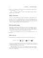
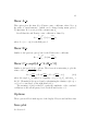
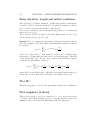
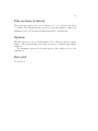
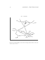
User manual for
Iode
(text-based interface)
Peter Brinkmann, Robert Jerrard, and Richard Laugesen
Department of Mathematics
University of Illinois, Urbana–Champaign, U.S.A.
March 5, 2010
2
Copyright (c) 2003, The Triode ([email protected])
Permission is granted to copy, distribute and/or modify this document under
the terms of the GNU Free Documentation License, Version 1.2 or any later
version published by the Free Software Foundation; with no Invariant Sections, no Front-Cover Texts, and no Back-Cover Texts. A copy of the license
is available at http://www.fsf.org/copyleft/fdl.html.
Contents
1 Direction fields
9
2 Phase planes
13
3 Second order linear ODEs
17
4 Fourier series
19
5 Partial differential equations
23
6 Purge temporary files
27
7 Quit
29
A Installing Iode
31
B Running Iode
33
C Reference materials
35
D Structure of Iode
39
3
4
CONTENTS
Overview
Iode (rhymes with diode) is a software package that enable students to explore direction fields, phase planes, second order linear ODEs, Fourier series
and heat and wave equations. The name Iode is supposed to be reminiscent
of “Illinois” and “ODE”.
Iode runs under either Matlab or Octave (their programming languages
are mostly compatible). For instructions on downloading, installing and
running all the needed software, see Appendix A. If your computer already
has Matlab or Octave installed, then all you need to get is Iode. Experienced
users can proceed directly to www.math.uiuc.edu/iode/ to download it.
The graphical user interface for Iode is supported only under Matlab,
version 6.0 or later. This manual describes the text-based user interface,
which runs under earlier versions of Matlab and also under Octave. The
graphical user interface offers certain features and plotting options that are
unavailable in the text-based interface.
A good way to learn Iode is simply to explore it. Choose various options
and see what happens. Also, the built-in help features in Matlab and Octave
are your friends. For example, typing help euler at the prompt will give
information on the module euler.m.
Please let us know if you encounter problems with Iode, or if you have
suggestions for improvement. To contact us, see www.math.uiuc.edu/iode/.
From a programming perspective, the main point of Iode is that it is modular and has well-defined interfaces. This has several useful consequences.
For example, it is easy for the user to customize Iode, or to create and plug in
new modules. Simple modules of this sort can be created even by users without much programming experience. In fact, Iode was born out of frustration
with other educational packages that conceal their inner workings from the
user.
The mathematical modules (such as df.m or euler.m) are usable in Mat5
6
CONTENTS
lab and Octave without the menus, and much of the code is easily extensible.
Users are encouraged, and in some of our classes expected, to look at the code
and modify it, take it apart, put it back together, and so on. For example,
Appendix D discusses how to create your own solver module for numerically
solving ODEs. On the other hand, Iode comes with a user interface that
exposes most of the capabilities of the mathematical modules, and so you
can use Iode even if you don’t have any programming skills. This manual
will mostly be concerned with explaining the user interface.
Iode main menu
After launching the text-based Iode user interface (see instructions in Appendix B), we get to the main menu:
[
[
[
[
[
[
[
1]
2]
3]
4]
5]
6]
7]
Direction fields
Phase planes
Second order linear ODEs
Fourier series
Partial differential equations
Purge temporary files
Quit
Before looking at these options in detail, we explain some features that
are common to all parts of Iode. For example, you will often be prompted to
input some piece of information (such as a number, or a variable name or a
function). Whenever this happens, Iode will display the current value of the
information inside square brackets. For example, the prompt
Independent variable [x]
asks you to input the name of the independent variable. The current name is
x, which is displayed inside square brackets. If in response you enter t (and
then hit return), t will be the name for the independent variable from then
on. If in response you do not enter anything but just hit return, then Iode
will simply keep using the current name x for the independent variable.
Iode also retains the current value if it cannot make sense of the information you provide. For example, a common mistake is to forget to type “*”
to indicate multiplication. If you are asked to enter a function and type 2xy
as 2xy, then Iode will report an error and will retain the previous function.
The correct expression is 2*x*y.
7
8
CONTENTS
The current value gives you a clue as to what kind of information Iode
wants from you. For example, if the current value is a number, then you
should probably enter a number. If the information that Iode seeks is not
a number but instead, say, a color code, then Iode will display a list of
acceptable responses.
Under Octave, Ctrl-D is a shortcut for quitting from any module in Iode,
or from Octave itself. More drastically, Ctrl-C will immediately terminate
Iode.
Chapter 1
Direction fields
This module deals with general first order ODEs, that is, equations of the
form
dy
= f (x, y).
(1.1)
dx
The module plots the associated direction (or slope) field in a separate graphics window, and it computes and plots numerical solutions of the equation.
The user can input the equation and the initial condition, and change the
method used for computing numerical solutions.
After selecting [ 1] from the Iode main menu, one sees the direction fields
menu; the menu options are explained below. The current ODE is always
displayed above the menu, along with the current values of the options for
the numerical method.
The graphics window shows a plot of the direction field for the ODE, with
the equation itself written across the top of the window.
When you first enter the module, you will find Iode has already chosen a
default ODE as well as reasonable option settings. Next we explain how to
change these settings.
Enter equation
When you select [ 1] Enter equation, you are prompted for three pieces of
information: an independent variable, a dependent variable, and a function.
When you input the names for the independent (horizontal) and dependent (vertical) variables, you are specifying the form in which you want the
equation written: for example,
9
10
CHAPTER 1. DIRECTION FIELDS
• dy/dx = f (x, y), in which case the solution will be a function y of a
variable x, or
• dx/dt = f (t, x), in which case the solution will be a function x of a
variable t.
In the first case you would input x for the independent variable and y for the
dependent variable. In the second case, input t for the independent variable
and x for the dependent variable.
Then Iode will prompt you to input the function f , using valid Matlab or
Octave syntax — consult Appendix C for examples. For example, to study
the equation dx/dt = xt2 , you should input x*t^2. Note that you do not
input the letter f, here. You just input the expression that you want on the
right hand side of the ODE.
Warning 1.1.
• Your expression for f should involve the independent or dependent
variables you have chosen (or both), but no other variables!
• Variable names should consist of only one letter, to avoid the risk of
conflicting with Iode’s internal variables.
Enter display parameters
Allows you to change the domain and range of the direction field, and the
number of line segments used to plot it. Note that this will clear all plots in
the graphics window.
The prompts are self-explanatory.
Plot numerical solution
dy
To get a specific solution of the differential equation dx
= f (x, y), you also
need to specify the initial data, y(x0 ) = y0 . When you select Plot numerical
solution, Iode asks you to input this information. Then you are asked to
input the color of the plot.
Remark 1.2. The algorithm and the step size used for actually computing
the numerical solution are displayed above the menu, and can be changed
using the next option.
11
Change numerical solver
When you select [ 4] Change numerical solver, you will be prompted for
the numerical method and step size. The step size should be a small, positive
number. Some acceptable choices for the numerical method will be listed on
the screen (or see Appendix C for more information on solvers).
Plot arbitrary function
If you know a formula for the exact solution of a differential equation, then
you might want to compare it with the numerical solution, which is only
an approximation, to see how accurate the numerical solution is. This helps
indicate how reliable the numerical solution will be on other problems, where
you do not know the exact solution.
The item [ 5] Plot arbitrary function allows you to plot the exact
solution. Actually it will plot any function for which you input the formula.
For example, to plot y = sin(x) you just input sin(x). Consult Appendix C
for more examples of functions you can use.
Clear plots
Clears all plots of functions from the graphics window, while leaving the
direction field intact.
Save plot
[This feature is only implemented for Octave because Matlab’s way of saving
plots is quite different. This shouldn’t be a problem, because Matlab’s user
interface has a menu item for saving plots.]
If you select [ 7] Save plot, you will be prompted for two pieces of
information: first a file name (without any extension), and then an extension.
For example, suppose that at the first prompt you enter my plot, and at the
second prompt you hit return to keep the default extension eps. Then a file
called my plot.eps will be created, containing your plot in a format known
as Encapsulated PostScript. To view or print your file, use the program
12
CHAPTER 1. DIRECTION FIELDS
Ghostview. For example, on a Unix system you would get to a Unix prompt
(outside of Octave) and type ghostview my plot.eps.
Remark 1.3. Only the graphics display is saved in the file, not the Iode
settings that generated it.
In the text-based user interface of Iode, there is no way to “save your
current settings” and come back to them later. (The graphical user interface
does offer this feature.)
For most purposes, you should use the default extension eps. Other valid
extensions include fig for Xfig pictures (choose this if you would like to
edit your plots with Xfig), gif for gif files (not recommended due to patent
issues), and png for Portable Network Graphics (choose this if you would like
to include your plots in web pages and such).
Warning 1.4. When you save a plot, if you enter the same name as an
existing file then the existing file will be overwritten, with no warning.
Chapter 2
Phase planes
This module deals with autonomous systems of two equations, that is, systems of equations of the form
dx
= F (x, y),
dt
dy
= G(x, y).
dt
(2.1)
The module creates a graphics window showing the phase portrait associated
with such a system, and it computes and plots numerical solutions of the
system in this phase plane. The user can input the system and the initial
conditions, and change the method used for computing numerical solutions.
After selecting [ 2] from the Iode main menu, one sees the phase planes
menu; the menu options are explained below. The current system of equations is always displayed above the menu, along with the current values of
the options for the numerical method.
The graphics window shows a plot of the phase portrait for the system,
with the system itself written across the top of the window.
When you first enter the module, you will find Iode has already chosen a
system and chosen the option settings. Next we explain how to change these
settings.
Enter functions
When you select [ 1] Enter functions, you will be prompted to input five
pieces of information: an independent variable, two dependent variables (the
horizontal and vertical variables), and the two functions F and G. Most
13
14
CHAPTER 2. PHASE PLANES
users will only work with autonomous systems, in which case the expressions
that you enter for F and G will involve only the dependent variables, not the
independent one.
Remark 2.1 (Note for advanced users). Iode can also handle nonautonomous
systems, in which the expressions for f and g depend also on the independent
variable t. Iode will correctly compute numerical solutions for such systems,
but will not draw the full phase portrait (which is three-dimensional). The
phase portrait that Iode displays in this case is the one at t = t0, see Section 2.
In all other respects, this option is similar to the corresponding part of
the direction fields module, described in Section 1.
Enter display parameters
Allows you to specify the region shown in the phase portrait, and to change
the number of line segments used to plot the phase portrait.
The prompts are self-explanatory. The parameter t0 is the value of the
independent variable for which the phase portrait is shown, and it is also the
initial value of the independent variable when computing numerical solutions.
Most users will only work with autonomous systems, in which case t0 doesn’t
matter.
Plot numerical solution
To get a specific solution of the system (2.1), you also need to specify the
initial data x0 = x(t0 ) and y0 = y(t0 ), which say where the plot should start in
the phase portrait. When you select [ 3] Plot numerical solution, Iode
asks you to input the initial data, and the t-duration of the plot. (Think of
the plot as tracing the path of a moving particle, in which case the t-duration
denotes the time elapsed.) The t-duration may be negative, in which case
the solution is computed backwards from t0 . You are also asked to input the
color of the plot.
Remark 2.2. The algorithm and the step size used for actually computing
the numerical solution are displayed above the menu, and can be changed
using the next option.
15
Change numerical solver
See Section 1.
Plot arbitrary trajectory
As in Section 1, this feature will be most useful in situations where you know
an exact formula for the solution, and want to compare it to a numerical
solution in order to estimate the accuracy of the numerical method.
Clear plot
See Section 1.
Save plot
See Section 1.
16
CHAPTER 2. PHASE PLANES
Chapter 3
Second order linear ODEs
This module deals with second order linear nonhomogeneous ODEs,
mx′′ (t) + cx′ (t) + kx(t) = f (t).
(3.1)
Equations of this sort arise in models of simple mechanical vibrations, and
electrical circuits. (Incidentally, the application to mechanical vibrations
explains why the module has filename mvmenu.m.)
The module plots the “forcing” function f , and it computes and plots numerical solutions of the equation (3.1). The user can input the equation and
the initial conditions, and change the method used for computing numerical
solutions.
After selecting [ 3] from the Iode main menu, one sees the Second order
linear ODEs menu; the menu options are explained below. The current ODE
is always displayed above the menu, along with the current values of the
options for the numerical method.
The graphics window shows a plot of the forcing function f , with the
equation itself written across the top of the window.
The options in this module are either self-explanatory or else are very
similar to the corresponding parts of the direction fields module.
Enter differential equation
When you select Enter differential equation, you will be prompted for
the six pieces of information needed to make sense of (3.1): an independent
and a dependent variable, the coefficients m, c and k (which are allowed to
17
18
CHAPTER 3. SECOND ORDER LINEAR ODES
involve the independent variable, but are usually just constants), and the
function f .
Otherwise this option is very similar to the corresponding part of the
direction fields module, described in Section 1.
Enter domain and range
See Section 1.
Plot numerical solution
See Section 1.
Change numerical solver
See Section 1.
Plot arbitrary function
See Section 1.
Clear plots
See Section 1.
Save plot
See Section 1.
Chapter 4
Fourier series
The Fourier series module can compute and graph the Fourier coefficients
of a periodic function f , and can plot partial sums of the Fourier series, as
well as the difference between the function f and partial sums of its Fourier
series. The user inputs the function f , decides how many coefficients are to
be computed, and can then “step through” the graphs of the partial sums.
For concreteness, here we will write f (x) for the function being considered,
even though the user can change the name of the independent variable from
x to something else, if desired.
After selecting [ 4] from the Iode main menu, you will see the Fourier
series menu and a graphics window. At the top of the graphics window, and
also above the Fourier series menu, you will see displayed a function f (x)
and the value of the “top harmonic”. The function is written in the form
f (x) = (a valid Matlab or Octave expression)
for x0 ≤ x < x1 , extended periodically, where x0 and x1 are numbers.
Remark 4.1. The interval x0 ≤ x < x1 is part of the definition of the
function! For example, it tells us that the period of the function is P =
x1 − x0 . See Section 4 for further discussion.
The graphics window shows a plot of f (in blue) over two periods. The
red plot is a partial sum of the Fourier series of f , that is, a plot of
N
A0 X
nπx
nπx
+
+ Bn sin
),
(An cos
2
L
L
n=1
19
(4.1)
20
CHAPTER 4. FOURIER SERIES
where N =“top harmonic”. Here An and Bn are the Fourier coefficients and
L is the half-period, L = (x1 − x0 )/2.
The “top harmonic” number N tells you the highest frequency that is
included in the partial sum.
Enter function
Select [ 1] Enter function to enter a new function. The function is the
periodic extension of a formula (given by the user) on an interval (given by
the user). So you are prompted not only for a formula for the function, but
also for the left and right endpoints of the interval. You are also given the
chance to change the name of the independent variable.
Plot partial sums
This displays partial sums of the Fourier series, in red in the graphics window.
Try hitting f (for “forward”) a few times and see how the display changes.
Notice that the value of the top harmonic (as shown in the graphics window)
goes up when you enter f, and goes down when you enter b.
Various options relating to these plots can be set using menu option [ 7]
Options.
Plot errors
This menu item is very similar to the previous one. It displays the error
#
N
A0 X
nπx
nπx
error(x) = f (x) −
+
+ Bn sin
)
(An cos
2
L
L
n=1
"
between f and partial sum of its Fourier series. The vertical scale of the plot
automatically adjusts to the size of the error, so that successive plots may
be displayed with different vertical scales.
Superimposing successive plots does not make sense if the scale changes,
and so this item will not superimpose plots, regardless of the plotting options
chosen in [ 7] Options.
21
Show A n
This option plots the first Nmax Fourier cosine coefficients, where Nmax is
the value of “max harmonic” (which can be changed using menu option [
7] Options). It does not plot the contant term A0 .
Recall that the nth Fourier cosine coefficient is defined by
Z
nπx
1 x1
dx,
f (x) cos
An =
L x0
L
where L = (x1 − x0 )/2 is the half-period.
Show B n
Similar to the previous option, but for the Fourier sine coefficients
Z
nπx
1 x1
f (x) sin
dx.
Bn =
L x0
L
Show C n=sqrt(A nˆ2+B nˆ2)
Similar to the previous
two options. The reason it is interesting to plot the
p
2
values of Cn = An + Bn2 is that
nπx
nπx
nπx
+ Bn sin
= Cn cos(
− αn ),
(4.2)
An cos
L
L
L
where the angle αn is defined by requiring cos αn = An /Cn and sin αn =
Bn /Cn . (Formula (4.2) is proved just by substituting the identity cos(β−α) =
cos β cos α + sin β sin α on the right hand side.)
The meaning of (4.2) is that Cn equals the amplitude of the combined
oscillations at the nth frequency level, in the Fourier series of f .
Options
These options all deal with aspects of the display. Play around and have fun.
Save plot
See Section 1.
22
CHAPTER 4. FOURIER SERIES
Chapter 5
Partial differential equations
This module computes and plots solutions of the wave equation and heat
(diffusion) equation. Solutions are found on an interval 0 ≤ x ≤ L, for times
0 ≤ t ≤ T . The method is separation of variables.
Enter equation and boundary conditions
When you select [ 1] Enter equation and boundary conditions, you
will be prompted first of all to choose either the heat equation
ut = kuxx
or the wave equation
utt = c2 uxx .
Heat (diffusion) equation. Then Iode asks for the diffusivity k, followed by
the boundary conditions. Iode can deal with Dirichlet boundary conditions
(u(0, t) = 0 and u(L, t) = 0), with Neumann boundary conditions (ux (0, t) =
0 and ux (L, t) = 0), and also with periodic boundary conditions (u(0, t) =
u(L, t) and ux (0, t) = ux (L, t)). Users are encouraged to create modules for
other boundary conditions as well: see dirichlet.m as a guide to doing this.
Wave equation. Then Iode asks for the wavespeed c, followed by the boundary conditions as above.
23
24
CHAPTER 5. PARTIAL DIFFERENTIAL EQUATIONS
Enter duration, length and initial conditions
After selecting [ 2] Enter duration, length and initial conditions,
you will be asked to enter the duration T over which the numerical solution
is to be plotted, and then the length L of the interval.
Heat equation. Then Iode asks for the initial temperature (or concentration)
function u(x, 0) = f (x).
Wave equation. Then Iode asks for the initial displacement u(x, 0) = f (x)
and the initial velocity ut (x, 0) = g(x).
Remark 5.1. Iode computes its approximate solutions by separation of variables. For example, for the heat equation with Dirichlet boundary conditions
Iode will use
N
max
X
nπx
2
u(x, t) =
bn e−(nπ/L) kt sin(
)
L
n=1
where Nmax is the value of “Max harmonic” (which can be changed using
menu item [ 6] Options), and where the bn are the Fourier sine coefficients
of the initial value f (x). For the wave equation with Dirichlet boundary
conditions the approximate solution is
u(x, t) =
N
max
X
n=1
nπct
nπct
nπx
L
bn cos(
) + Bn
sin(
) sin(
),
L
nπc
L
L
where the bn are the Fourier sine coefficients of the initial displacement f (x)
and the Bn are the Fourier sine coefficients of the initial velocity g(x).
Plot 3D
This plots the graph z = u(x, t) of the approximate solution, in 3- dimensions.
Plot snapshots (t-slices)
This plots the graph of u(x, t) as a function of x, for a discrete succession
of t-values. The default plotting option is to step through the t-values, but
animation can be chosen instead using menu item [ 6] Options.
25
Plot sections (x-slices)
This plots the graph of u(x, t) as a function of t, for a discrete succession
of x-values. The default plotting option is to step through the x-values, but
animation can be chosen instead using menu item [ 6] Options.
Options
The first option is to choose Max harmonic Nmax , which specifies how many
terms to take in the Fourier series that are used to construct approximate
solutions.
The remaining options all deal with aspects of the display, and are selfexplanatory.
Save plot
See Section 1.
26
CHAPTER 5. PARTIAL DIFFERENTIAL EQUATIONS
Chapter 6
Purge temporary files
Unfortunately, Octave and Gnuplot generate a large number of temporary
files, and they don’t always remove these files properly. A prolonged Iode
session (or a session involving extremely complex plots) can then fill up your
file system with temporary files. This is a known problem of Octave and will
be corrected in a future version.
If Octave has accumulated too many temporary files, your plots will be
left incomplete or might not get updated correctly. You can fix the problem
by exiting to the main menu and choosing [ 6] Purge temporary files.
After deleting the temporary files, you can continue your work with Iode.
If you are using Octave and Gnuplot without the user interface of Iode,
it may be a good idea to remove temporary files every once in a while by
issuing the command purge tmp files.
27
28
CHAPTER 6. PURGE TEMPORARY FILES
Chapter 7
Quit
This quits out of Iode, returning the user to an Octave prompt.
Incidentally, when running Iode under Octave, Ctrl-D is a shortcut for
quitting out of any module or out of Octave itself. More drastically, Ctrl-C
will immediately terminate Iode.
29
30
CHAPTER 7. QUIT
Appendix A
Installing Iode
Iode runs under either Matlab or Octave. If you wish to use the graphical
user interface of Iode, you will need Matlab Version 6.0 or later.
If your computer already has Matlab or Octave installed, then you only
need to install Iode.
Obtaining and installing Iode
On your machine, create a directory called my iode or similar. Then. . .
• Unix systems: From www.math.uiuc.edu/iode/, download the file
iode.zip and unpack it into the directory my iode with unzip or similar.
• Windows systems: From www.math.uiuc.edu/iode/, download the file
iode dos.zip and unpack it into the directory my iode with WinZip
or similar.
Iode is free software, available under the GNU General Public License.
Obtaining and installing Matlab
Matlab is commercial software, available at www.mathworks.com for Unix,
Windows and Mac. It is already installed on many Unix systems in universities. Matlab is available to students at a discounted price (see the downloads
page at www.math.uiuc.edu/iode/).
31
32
APPENDIX A. INSTALLING IODE
After installing Matlab on a Windows system, it is helpful to set it up to
launch in the correct directory. See Appendix B.
Obtaining and installing Octave
Octave is free software, and you can obtain it from www.octave.org for Unix,
Windows, and Mac OS X.
Installing Octave on Unix systems
If your home machine runs Unix, then chances are that you are already expert
enough to download and install Octave yourself, following the directions at
www.octave.org. If you run into trouble, your local Unix geeks will be happy
to help.
Installing Octave on Windows systems
You can find an easy to install Windows executable at
http://www.site.uottawa.ca/~adler/octave/.
After downloading the .exe file, chances are that your browser will offer
to run the installation program. If not, then you should double-click on the
file to activate the installation.
If something goes wrong with the installation of Octave, you may be able
to get some help at http://octave.sourceforge.net/Octave Windows.htm.
After installing Octave under Windows, it is helpful to set it up to launch
in the correct directory. See Appendix B.
Appendix B
Running Iode
Running Iode under Unix
Log in to the machine and get to a Unix prompt. Change directory to get
into my iode by using a Unix command such as cd my iode. Then launch
Matlab or Octave by typing matlab or octave at the prompt. Note that
the order of operations matters here: you need to change into the directory
containing Iode before you launch Matlab or Octave.
Once you have gotten Matlab or Octave running, just type iode at the
Matlab or Octave prompt. The graphical user interface for Iode will launch
if it can; otherwise the text-based user interface will launch. Some development versions of Octave sometimes fail to work with the part of Iode that
determines whether the graphical user interface can be launched. If you are
using a version of Octave that reports an error when processing the command
iode, you can launch the text-based interface right away, by typing iodetxt.
Running Iode under Windows
Log in to the machine and launch Matlab or Octave through the Start →
Programs menu.
Remark B.1 (Important note). Before launching Matlab or Octave for
the very first time, it is helpful to right-click on the program name in
the Start → Programs menu, then click on Properties, and put the correct filepath into the “Start in:” box. Your filepath should look something
33
34
APPENDIX B. RUNNING IODE
like C:\My files\MathClass\my iode. The point is that from now on, when
you launch Matlab or Octave it will be able to find the iode files.
Once you have gotten Matlab or Octave running, just type iode at the
Matlab or Octave prompt. If this does not work, then you probably need to
change into the directory my iode where you have stored the Iode files. You
can do this from within Matlab or Octave, using Unix commands such as cd
my iode, at the Matlab or Octave prompt.
Appendix C
Reference materials
Mathematical expressions in Matlab, Octave
and Iode
For simple expressions, we use the usual keyboard characters:
2*x
means 2x,
(x^3-1)/6 means (x3 − 1)/6.
Or instead of the usual division /, we can use “left division” \.
pi/3
3\pi
means π3 ,
also means π3 .
Built-in functions
exp(x)
log(x)
log10(x)
abs(x)
sqrt(x)
sign(x)
sin(x)
exponential, ex
natural logarithm, ln x
base 10 logarithm, log10 x
absolute value,
√ |x|
square root, x

 +1 if x > 0
0 if x = 0
signum function, which equals

−1 if x < 0
sinh(x)
35
36
APPENDIX C. REFERENCE MATERIALS
cos(x)
tan(x)
cot(x)
sec(x)
csc(x)
trigonometric
functions
(x in radians)
cosh(x)
tanh(x)
coth(x)
sech(x)
csch(x)
hyperbolic
trigonometric
functions
asin(x)
asinh(x)
acos(x) inverse
acosh(x) inverse
atan(x) trigonometric
atanh(x) hyperbolic
acot(x) functions
acoth(x) trigonometric
asec(x)
asech(x) functions
acsc(x)
acsch(x)
besselj(nu,z)
Bessel function of the first kind
bessely(nu,z)
Bessel function of the second kind
besseli(nu,z)
Modified Bessel function of the first kind
besselk(nu,z)
Modified Bessel function of the second kind
Example C.1.
sin(exp(y))^4
acos(exp(1)^(-1))
means sin4 (ey ),
means arccos(e−1 ).
No matter whether you’re using Octave or Matlab, you can always find
more information on a function by typing help function.
Additional Iode functions
The installation of Iode includes the following functions, useful for studying
Fourier series and for creating initial values for partial differential equations.
hat(x,a,b): equals 0 for x ≤ a and x ≥ b, and equals 1 for a < x < b.
To make sense, hat requires a < b.
triangle(x,a,b,m): a triangular-shaped function, equalling 0 for x ≤ a,
then rising linearly to height 1 at x = m and falling back linearly to zero
at x = b, then equalling zero for x ≥ b. To make sense, triangle requires
a < m < b. The parameter m is optional and defaults to the midpoint a+b
.
2
37
bump(x,a,b,m): is a continuously differentiable function that equals 0
for x ≤ a and x ≥ b, is positive for a < x < b, has a maximum of 1 at x = m,
and is strictly increasing between a and m and strictly decreasing between
m and b. To make sense, bump requires a < m < b. The parameter m is
optional and defaults to a+b
.
2
Logical expressions in Matlab, Octave and Iode
Expressions like x>=2 are treated as logical functions, and return a value
of either 1 (true) or 0 (false). So x>=2 is the “step” function that equals
1 if x ≥ 2
.
0 otherwise
Example C.2. Logical functions help us create functions defined in pieces:
(t^2)*(t<4)
means
t2 if t < 4
,
0 otherwise
because (t<4) equals 1 if t < 4 and equals 0 otherwise.
Color codes recognized by Matlab, Octave and
Iode
b
g
r
c
m
y
k
blue
green
red
cyan
magenta
yellow
black
Note that yellow plots are usually hard to see due to lack of contrast.
38
APPENDIX C. REFERENCE MATERIALS
Some solver codes recognized by Iode
euler
rk
Euler method for (systems of) first order equations
Runge–Kutta for (systems of) first order equations
In addition to the pre-installed solvers listed above, you can also create
your own. For example, if you devise a new method for solving differential
equations, then you could program it in a new file called my algorithm.m,
in your Iode directory. The structure of my algorithm.m should follow that
of euler.m. You will simply need to change the “update” steps, which in
euler.m are:
k1=feval(fs,x,tc( i ));
x=x+h∗k1;
Then after creating the file my algorithm.m, you can input my algorithm
when Iode prompts you for a numerical method.
Appendix D
Structure of Iode
For users who like to look under the hood, we now provide some information
on the structure of Iode. We encourage users to modify Iode and create new
modules.
Figure D.1 breaks Iode down into its constituent modules. Each module
occurs as an m-file with the same name. For example, dfmenu in the figure
means the file dfmenu.m that comes as part of the Iode package.
There are two kinds of module. The first kind are the menus and auxiliaries, providing the user interface. The second (and main) kind are the
mathematical modules, which actually perform the calculations needed to
solve the differential equations numerically, and calculate the Fourier coefficients numerically, and so on.
The mathematical modules euler.m and rk.m are particularly instructive
— they implement the Euler and Runge–Kutta methods for solving a first
order ODE. You can implement different solver methods yourself, as outlined
in Appendix C.
In order to develop a better understanding of what the various modules
do, you can look at the file doc.txt. Together with Figure D.1, it should
give you a rather complete picture of the structure of Iode. Another useful
file to look at is sample.m, which contains the transcript of a short Octave
session that shows how to use the direction fields module and numerical
solvers without resorting to any menus.
Any manual can only take you so far. If you have followed this manual
up to this point, you are ready to go exploring on your own. Good luck, and
have fun!
39
40
APPENDIX D. STRUCTURE OF IODE
Iode −−− Text Version
df
euler
solplot
pp
dfmenu
rk
ppmenu
trajplot
mvmenu
iodetxt
partialsum
fsmenu
mp
slideshow
dirichlet
choose
neumann
fs
pdemenu
wave
cosef
coeff
trapsum
heat
periodicef
sinef
periodic
Figure D.1: Relationships between the most important modules of the textbased version of Iode.