Download Medicina User Manual THE RADIOTELESCOPE

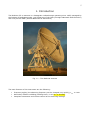
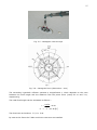
Medicina User Manual
32-m Antenna
Version 1
Elena Cenacchi
Alessandro Orfei, Karl-Heinz Mack, Giuseppe Maccaferri
[email protected]
THE RADIOTELESCOPE
Last update : 20 April 2006
2
3
Index
1 – INTRODUCTION............................................................................................
5
2 – ANTENNA STRUCTURE ..................................................................................
2.1 Azimuth rail ...............................................................................................
2.2 Primary reflector.........................................................................................
2.3 Quadrupod and secondary reflector ...............................................................
2.3.1 Wobbling ...........................................................................................
2.4 Pointing errors ...........................................................................................
2.5 Specification summary ................................................................................
2.5.1 Observation conditions .........................................................................
2.5.2 Surface accuracy.................................................................................
2.5.3 Pointing errors ....................................................................................
7
7
7
8
10
10
11
11
11
12
3 – OPTICS.........................................................................................................
3.1 Primary focus .............................................................................................
3.2 Cassegrain focus.........................................................................................
3.3 Servosystem specifications...........................................................................
13
13
14
16
4 – FRONT END ..................................................................................................
4.1 Feeds and receivers ....................................................................................
1.4/1.6 GHz................................................................................................
2.3/8.3 GHz................................................................................................
5 GHz ........................................................................................................
6 GHz ........................................................................................................
22 GHz ......................................................................................................
4.2 Distributions ..............................................................................................
4.3 Control room..............................................................................................
19
20
21
23
25
28
31
32
33
5 – EFFICIENCY AND SYSTEM TEMPERATURE ..................................................... 35
6 – VLBI ............................................................................................................. 37
7 – OBSERVING MODES ...................................................................................... .
7.1 ON-OFF techniques .....................................................................................
7.2 Mapping techniques ....................................................................................
7.3 Pulsar .......................................................................................................
39
39
39
41
8 – BACK END..................................................................................................... .
8.1 Spectrometers............................................................................................
8.1.1 Arcos.................................................................................................
8.1.2 Mspec0 ..............................................................................................
8.2 Continuum.................................................................................................
8.2.2 Mark IV .............................................................................................
8.3 Polarimeter ................................................................................................
8.4 Pulsar .......................................................................................................
8.4.1 SPEX .................................................................................................
8.5 VLBI .........................................................................................................
8.5.1 Mark IV .............................................................................................
8.5.2 e-VLBI ...............................................................................................
43
44
44
45
46
46
48
49
49
50
50
50
9 – REMOTE CONTROL ........................................................................................ 53
APPENDIX – HOW TO READ THE CALIBRATION TEXT FILES ................................ 55
4
5
1. Introduction
The Medicina 32 m antenna is a Cassegrain radiotelescope operating since 1983, managed by
the Istituto di Radioastronomia, until 2004 part of the CNR (Consiglio Nazionale delle Ricerche)
and now part the INAF (Istituto Nazionale di AstroFisica).
Fig. 1.1 : The Medicina antenna
The main features of this instrument are the following :
•
•
•
Frequency agility (the observing frequency can be changed very quickly), tmax ≤ 4 min
Secondary reflector wobbling (shifting time ≤ 1 sec at ν ≥ 20 GHz)
Complete automation and remote control of the observing settings
6
Position
Medicina (BO), Italy
Coordinates
Lat. 44°31'15" N - Long. 11°38'49" E - Alt. 25 m f.s.l.
Optics
Cassegrain
Frequency coverage
1.4 ÷ 22 GHz
Primary reflector diameter
32 m
Secondary reflector diameter
3.2 m
Available foci
Primario f/D = 0.32
Cassegrain f/D = 3.04
Elevation range
0°÷90°
Azimut range
± 270°
Slew rates (wind speed < 60 km/h)
48°/min Azimuth
30°/min Elevation
Surface accuracy (rms specified)
0.6 mm*
Pointing accuracy (rms specified)
8 arcsec
FWHM Beamwidth
38.7 arcmin/f (GHz)
Gain
0.10 ÷ 0.16 K/Jy
First secondary lobes
≈ 20 dB under the main lobe
Receivers mounts
Primary focus : movable positioner (3 receiver bays)
Cassegrain focus : fixed (9 receiver bays)
Tab. 1.1 : Characteristics of Medicina's antenna
* 60° Elevation
Fig. 1.2 : Medicina's antenna, side
7
2. Antenna Structure
2.1 Azimuth Rail
The whole antenna leans upon the azimuth rail, which has a 18.3 m diameter and has recently
(2001) been renewed. Until 2000 the rail was directly substained by the grout basement (see
fig. 2.1)
Fig. 2.1 : First solution
Then a more efficient solution, in terms of endurance, was proposed, and a metal plate was
interposed between the rail and the grout basement. Moreover, a new kind of grout, a reinforced grout, wa
Fig. 2.2 : Installation of the metal plate (antenna lifted) and
finished work (the plate and the basement are both white painted)
2.2 Primary Reflector
The primary reflector. diameter 32 m, is made of 240 aluminium panels (RMS = 0.4 mm)
substained by a backup reticular truss. The housing of the Cassegrain focus feeds is at the
mirror vertex.
8
Fig. 2.3 : Primary reflector, front
C1
(mm)
D1
(mm)
D2
(mm)
Raw B
2617.8
437.62
1113.96
Raw C
2604.15
1113.96
1770.4
Raw D
2617.24
887.1
1206.06
Raw E
2648.38
1206
1515
Raw F
2659.33
1515.04
1810.74
Raw G
2718
1810.74
2098.14
Tab 2.1 : Geometry of the panels
2.3 Quadrupod and Secondary Reflector
The primary reflector backup structure substains the secondary mirror, placed at a distance of
9 m, through 4x45° inclined beams (quadrupod).
9
The secondary mirror is a hyperbolic reflector, 3.2 m diameter, made of a single aluminium
panel (rms = 0.35 mm). On the backup structure 3 mechanical actuators are installed and
allow the mirror to tilt around the 3 axis. Besides the whole system can translate along the x
and y axis.
Fig. 2.4 : Hyperbolic mirror
The mirror must completely be retracted along the y axis when the primary focus is used.
Fig. 2.5 : Configuration for Cassegrain focus usage (plain line) and primary focus usage
(dotted line)
The mirror and the quadrupod induces an obstruction on the primary reflector of nearly 4%.
Cause
Obstruction
Sub-reflector
2%
Quadrupod
2%
Total
4%
Tab. 2.2 : Primary reflector obstruction
10
2.3.1 Wobbling
The system that rotates the secondary mirror has been optimized in order to enhance the
number of receivers that can be installed at the Cassegrain focus.
Anyway, for the receivers installed in the external circumference, the same movement can be
used for the Wobbling technique. Typical shifting times, quite more advantageous if compared
with the Position Switching technique, are listed in the following table.
Frequency Beam HPBW
(GHz)
(“)
Mirror rotation
Mirror rotation
Required time
Required time
2.5 beam
5 beam
(sec)
(sec)
(°)
(°)
5
450
2.56
1.16
5.12
2.12
6
390
2.22
1.03
4.44
1.86
22
120
0.68
0.45
1.37
0.71
Tab. 2.3 : Wobbling time for 2.5 beam and 5 beam
2.4 Pointing Errors
The accuracy of the pointing correction increases with the observing frequency, i.e. as the
antenna beam width decreases.
It is commonly assumed the following :
δp =
HPBW
10
δp = pointing accuracy
HPBW = -3 dB beam width (main lobe)
For the Medicina antenna the values are listed in the following :
Frequency HPBW Error
(GHz)
(')
(')
1.5
29
≤ 2.9
22
2
≤ 0.2
Tab. 2.4 : Beam and pointing errors
The systematic errors are usually quite high (some arcminute). Anyway they have been
determined according to the antenna position (Az/El) after apposite astronomical observations
(reference radio sources) and a correction model has been derived.
Once the model has been applied, the residual error is 0.13' (both in azimuth and elevation),
exactly as required.
11
2.5 Specification Summary
2.5.1 Observation conditions
Parameters
Precision
Normal
Survival
Specifications
Wind, continuous
Wind, gusts
< 25 km/h
20÷ 30 km/h
Sun
Absent
Precipitation
Absent
Temperature
-25 ÷ 30 °C
Humidity
< 90 %
Wind, continuous
Wind, gusts
< 65 km/h
50 ÷ 80 km/h
Precipitation
Absent
Temperature
-30 ÷ 50 °C
Humidity
< 100%
Wind
200 km/h
Precipitation
< 5 cm/h snow
Seismic
0.3 g horizontal
Tab. 2.5 : Observation conditions
In survival conditions, and when not in use, the antenna must be settled at 90° elevation and
180° azimuth (stow position).
2.5.2 Surface Accuracy
(RSS mm) (RSS mm)
90° El
60° El
Structural Elements
Primary reflector panels
0.4
0.4
Secondary reflector panels
0.35
0.35
Gravitational deformation
0.58
0.19
0.8
0.6
Total surface accuracy
Tab. 2.6 : Surface accuracy at 90° and 60° elevation
To estimate the phase error from the surface accuracy, the following can be used :
ε =
δ = surface accuracy
λ = observation wavelength
4πδ
λ
[rad]
12
Usually a maximum tolerable phase error is assumed as ε≈36°≈0.63 rad , so that the
minimum observable wavelength is
λmin ≈ 20δ max
For the Medicina antenna :
λ min ≈ 16 ÷ 12 mm → ν max ≈ 19 ÷ 25 GHz
2.5.3 Pointing accuracy
E' IN ITALIANO!!
Condizione di osservazione
Precisione di puntamento
(rms arcmin)
Normale/Precisione
0.13
Tab. 2.6 : Precisione di puntamento
13
3. Optics
The Medicina antenna has 2 focal positions :
•
•
Primary focus : F1
Cassegrain focus : F2
Fig. 3.1 : Optics of Medicina antenna [dimensions : mm]
3.1 Primary Focus
With the Cassegrain optic the primary reflector focus is usable only if the secondary reflector is
completely retracted. Behind the mirror a movable positioner is installed, equipped with 3
receiver bays.
Fig. 3.2 : Primary focus feed positioner
14
The primary mirrror focal length is nearly 10.3 m, therefore the focal ratio is F1/D ≈ 0.32.
Fig. 3.3 : Primary focus (dimensions : mm)
3.2 Cassegrain Focus
The secondary mirror (9 m from the primary mirror) allows the usage of the Cassegrain focus
(at nearly 20 cm above the reflector's vertex)
This focus has been studied to offer more adjacent focal positions, which can be obtained
through the angular movement of the secondary mirror (see fig. 3.4).
Fig. 3.4 : Cassegrain focal plane
At this focus, 9 receivers can be mounted (a central one plus eight around).
15
Fig. 3.5 : Cassegrain receiver bays
Fig. 3.6 : Cassegrain focus (dimensions : mm)
The secondary hyperbolic reflector operates a magnification i2 which depends on the ratio
between the focal length and the distance from the prime focus (nearly 20 m and 3 m,
respectively).
The total focal length can be estimated as follows :
9.074
≈ 9.49
0.956
F2 = i 2 ⋅ F1 ≈ 97.36 [m]
i2 =
The focal ratio is therefore: F2 / D ≈ 3.04
By now at this focus the 5 GHz and 6 GHz receivers are installed.
16
3.3 Servosystems Specifications
Azimuth drive
Angular travel
Kinematics
Angular velocity
Angular acceleration
Configuration
Track
Unity
Value
(°)
540
(°/sec)
2
0.8
(°/sec )
0.82
Number of wheels
(-)
4
Driving wheels
(-)
2
Drives per wheel
(-)
1
Diameter
(m)
18.3
Unity
Value
(°)
90
Tab. 3.1 : Azimuth drive
Elevation drive
Angular travel
Kinematics
Angular velocity
Angular acceleration
(°/sec)
0.5
2
(°/sec )
0.31
Unity
Value
(mm)
420
Tab. 3.2 : Elevation Drive
Primary focus feed positioner
Linear travel
Kinematics
Linear velocity
Linear acceleration
(mm/sec)
2
(mm/sec )
7.2
24
Tab. 3.3 : Primary focus feed positioner, transverse axis
Primary focus feed positioner z axis
Linear travel
Kinematics
Linear velocity
Linear acceleration
Unity
Value
(mm)
350
(mm/sec)
2
(mm/sec )
Tab. 3.4 : Primary focus feed positioner, z axis
7.2
24
17
Sub-reflector
Kinematics
Unity
Value
Linear travel x axis
(mm)
160
Linear travel y axis
(mm)
160
Linear travel y axis out of focus
(mm)
2240
Linear travel z axis
(mm)
250
Angular travel x axis
(°)
±4.2*
Angular travel y axis
(°)
±4.2*
Linear velocity x axis
(mm/sec)
55.5
Linear velocity y axis
(mm/sec)
17.1
Linear velocity z axis
(mm/sec)
48.3
(°/sec)
1.9
Angular velocity
Tab. 3.5 : Sub-reflector kinematics
18
19
4. Front End
The Medicina antenna covers the range 1.35÷24.1 GHz. As shown in the following scheme, the
receivers installed in the primary focus (1.4/1.6, 2.3-8.3, 22 GHz) share some electronic parts (the
single sections dedicated to the receivers show the connection lines for each frequency).
Fig. 4.1: Primary focus receivers scheme
The Cassegrain focus receivers are currently being updating and will soon be substituted with
the wider band system developed for the Sardinia Radio Telescope (the 6 GHz receiver will be
included in the new 7 GHz system).
The taper levels are the following :
Frequency Taper
(GHz)
(dB)
1.4/1.6 -17
2.3
-16
5
-10
6
-14
8.3
-16
22
-15
Tab. 4.1 : Taper levels
20
4.1 Feeds and Receivers
The following receivers are available (click on frequencies for detalis) :
Band
ν0
λ
(Name) (GHz) (cm)
L
1.4
21
L
1.6
18
S
2.3
13
C
5
6
C
6
5
X
8.3
3.6
K
22
1.3
Receiver
N°
Beam (')
Noise
νLsky νHsky Receivers
Calibration
Configuration
band
temperature
Info
N/S E/W (GHz) (GHz)
(MHz)
(K)
lhp
31.0 31.3
llp
27.5 27.6 1.595 1.715
ssp or sxp* 18.6 17.3
1.35
1.45
2x80
50
2x80
60
2.20
2.36
2x160
40
ccc
7.50 7.40
4.65
5.15
2x350
44
chc
7.00 6.50
5.90
7.10
2x400
57
xxp or sxp* 4.80 5.00
8.18
8.98
2x800
25
2x800
80
kkp
2.00 2.00 21.86 24.14
LH
LL
Coxial 8.3 GHz
SS
CC
CH
Coaxial 2.3 GHz
XX
KK
Tab. 4.2 : Receivers parameters
*Name related to the coaxial use
Primary Focus
Cassegrain Focus
νLsky ÷ νHsky : receiver maximum bandwidth
The receivers label has been assigned only for identification purpose (the p and c letters
stands for primary and Cassegrain focus respectively).
HOW TO READ THE CALIBRATION TEXT FILES (See Appendix)
At 1.4, 1.6, 2.3 GHz available bandwidths may be considered less then what reported because
of interferences.
Multifrequencies observations can be conducted by quick receiver changes (frequency agility):
LL/LH
LL/LH
SX/SS/XX
CC
CH
KK
46 sec
3 min 20 sec
3 min 20 sec
22 sec
3 min 25 sec
3 min 25 sec
26 sec
3 sec
3 min 21 sec
SX/SS/XX
46 sec
CC
3 min 20 sec
3 min 25 sec
CH
3 min 20 sec
3 min 25 sec
3 sec
KK
22 sec
26 sec
3 min 21 sec
3 min 21 sec
3 min 21 sec
Tab. 4.3 : Switching times between receivers (COLORI DIVERSI?)
21
1.4/1.6 GHz
Type
Hot
Channels
2
Polarization
LHC-RHC
Central frequency (GHz)
1.406
1.665
Noise temperature
50 K
60 K
Useful RF band (GHz)
1.35÷1.45
1.595÷1.715
RF filter width (MHz)
100
120
IF filter width (MHz)
80
80
Istantaneous RF band (GHz) 1.366÷1.446 1.625÷1.705
OL frequency (GHz)
OL range (GHz)
Conversion (GHz)
1.036
1.295
1.020÷1.040 1.265÷1.305
Single USB
0.33÷0.41
Standard parameters of the 1.5 GHz parameters
The maximum bandwidth is 80 MHz, tunable only within the two RF ranges listed in the above
table. To shift the IF standard band inside the RF band of Δν, the OL frequency must be
changed (within the range listed in the table) according to the following :
RF = 1.350 ÷ 1.450 → ν OL = 1.036 ± Δν
RF = 1.595 ÷ 1.715 → ν OL = 1.295 ± Δν
1.4 GHz receiver scheme (green lines)
22
1.6 GHz receiver scheme (green lines)
At 1.4, 1.6 GHz available bandwidths may be considered less then what reported because
of interferences.
23
2.3-8.3 GHz
Type
Cooled Coaxial
Canali
2
Polarization
Central frequency (GHz)
Noise temperature
Useful RF band (GHz)
LHC-RHC
LHC-RHC
2.28
8.58
40
25
2.20÷2.36 8.18÷8.98
RF filter width (MHz)
160
800
IF filter width (MHz)
160
800
Istantaneous RF band (GHz) 2.20÷2.36 8.18÷8.98
OL frequency (GHz)
OL range (GHz)
Conversion (GHz)
2.020
8.080
0
0
Single USB Single USB
0.18÷0.34 0.1÷0.9
Standard parameters of the 2.3-8.3 GHz coaxial receiver
It is possible to use the receivers both together (coaxial, 2 IF outputs, one per each frequency)
and separately (2 IF outputs). For the VLBI coaxial observation one channel only for each
receiver is used, typically the right polarization one (this because the Mark IV can handle only
2 IF inputs).
2.3 GHz receiver scheme (green lines)
24
8.3 GHz receiver scheme (green lines)
At 2.3 GHz available bandwidths may be considered less then what reported because
of interferences.
25
5 GHz
Type
Cooled
Channels
2
Polarization
LHC-RHC
Central frequency (GHz)
4.875
Noise temperature
44
Useful RF band (GHz)
4.65÷5.15
RF filter width (MHz)
500
IF filter width (MHz)
350
Istantaneous RF band (GHz) 4.700÷5.050
OL frequency (GHz)
OL range (GHz)
1.150x4
1.138÷1.175
Single USB
0.1÷0.45
Conversion (GHz)
Standard parameters of the 5 GHz receiver
To shift the IF standard band inside the RF band of Δν, the OL frequency must be changed
(within the range listed in the table) according to the following :
ν OL =
4.600 ± Δν
4
This receiver will be soon updated (the band will become wider). The following conversion
scheme is related to the new receiving system.
5 GHz receiver scheme
26
Receiver mounted : 5 GHz (on the left) and 6 GHz (on the right)
Conversions scheme
27
5-7 GHz converter
28
6 GHz
Type
Hot
Channels
2
Polarization
LHC-RHC
Central frequency (GHz)
6.1
Noise temperature
6.7
57
Useful RF band (GHz)
5.90÷7.10
RF filter width (MHz)
1200
IF filter width (MHz)
400
Istantaneous RF band (GHz) 5.90÷6.30 6.50÷6.90
OL1 frequency (GHz)
8.10
8.70
OL2 frequency (GHz)
2.30
2.30
OL1 range (GHz)
8.10÷9.30
Conversion (GHz)
Double LSB
1.80÷2.20
0.1÷0.5
Standard parameters of the 6 GHz receiver
To shift the IF standard band inside the RF band of Δν, the OL frequency must be changed
(within the range listed in the table) according to the following :
ν OL = 8.10 ± Δν
This receiver will be soon updated(??)(the band will become wider and the central frequency will
be 7 GHz). The following conversion's scheme is related to the new receiving system.
7 GHz receiver scheme
29
Receiver mounted
Conversion scheme
30
5-7 GHz converter
31
22 GHz
Type
Cooled
Channels
2
Polarization
LHC-RHC
Central frequency (GHz)
22.464
Noise temperature (K)
80
Useful RF band (GHz)
21.86÷24.14
RF filter width (MHz)
2300
IF filter width (MHz)
800
Istantaneous RF band (GHz) 22.064÷22.864
OL1 frequency (GHz)
1.7355 (x8)
OL2 frequency (GHz)
8.080
OL1 range (GHz)
1.710÷1.945
Conversion (GHz)
Double USB
8.18÷8.98
0.1÷0.9
Standard parameters of the 22 GHz receiver
To shift the IF standard band inside the RF band of Δν, the OL frequency must be changed
(within the range listed in the table) according to the following :
ν OL =
(21.964 ± Δν ) − 8.080
8
Schema del ricevitore a 22 GHz (evidenziato in verde) E' IN ITALIANO
32
4.2 Distribution
The connections between the radiotelescope's foci involve three different kinds of signal :
. Local Oscillator : in order to cut down the expenses related to the construction of an high
number of independent superheterodyne recevers, a very common solution is to share some
local oscillators (at least for one conversion). A single local oscillator therefore can serve more
receivers through a signal distribution system.
. IF : the RF signals, once received and converted by the Front End, are sent to the Back End
installed in the Control Room, at the antenna's base.
. Reference : 5 MHz H-maser signal, necessary for the local oscillator stability.
All the signals are distributed via coaxial cable.
The distribution scheme is simplified by the fact that there are only two double conversion
receivers (6 GHz at the Cassegrain focus and 22 GHz at the primary focus) and both use the
same local oscillator for the second conversion. Besides the two receivers' channels can't be
placed in different position inside the RF bandwidth.
The OL signal is distributed by and OL distributor (OLD).
The reference distributor (REFD) and the IF distributor (IFD) are also installed at the
Cassegrain focus. From the control room it is possible to choose the receiver through the
selector.
Fig. 4.2 : Signal distribution between the foci
33
Fig. 4.3 : Distributors : reference signal (on the left) and local oscillator (on the right)
4.3 Control Room
The backend systems are installed in the control room, located at the antenna's base. It is
connected to the foci through the links shown in the following (red line and green line are fiber
optic links) :
Fig. 4.3 : Control links
From the control room it is possible to act on receivers, antenna's movement and subreflector's movement. Besides it will be possible to interact with the new metrology system
(temperature sensors and a little optical telescope installed at the Cassegrain focus) projected
for SRT and that will be tested on the Medicina's antenna
The control room is part of the Observatory LAN (at nearly 500 meters from the antenna).
34
35
5. Efficiency and System Temperature
The antenna gain is defined as :
mη A Ag
G = 10 −26
⎡K ⎤
⎢ ⎥
⎣ Jy ⎦
kB
m = 0.5 (non polarized radiation)
Ag = geometric area
kB = Boltzmann's constant
ηA = antenna efficiency
For the Medicina antenna, the constants are :
10 −26
Ag
2 ⋅ kB
≈ 0.292
ηA is the overall efficiency, estimated assembling all the signal degradation factors.
The antenna gain varies according to the elevation and it reaches a maximum at 45°. A good
interpolation is obtained with a second degree curve, such as :
ax 2 + bx + c
The coefficients of the normalized polynomials, at each frequency, are listed in the following :
Frequency
(GHz)
a
b
c
1.4
-6.8310687·10-5
7.285044·10-3
8.0577027·10-1
1.6
-2.6828893·10-5
3.4836402·10-3
8.869153·10-1
2.3
-1.3256035·10-4
1.7229174·10-2
4.4017117·10-1
5
-5.3473118·10-5
6.0312044·10-3
8.2993592·10-1
6
-5.8197959·10-5
9.4270958·10-3
6.1824204·10-1
8.3
-7.2457279·10-5
1.0623634·10-2
6.1059261·10-1
22
-2.4658337·10-4
2.0935913·10-2
4.4252013·10-1
Tab. 5.1 : Normalized gain curves, coefficients
FROM THIS PAGE IT IS POSSIBLE THE DOWNLOAD OF THE UPDATED CALIBRATION FILES
36
The sensitivity can be estimated as follows :
ΔS =
αT sys
G Δν τ nN IF
 = receiver constant (=1)
Tsys = system temperature
G = gain (K/Jy)
Δν = bandwidth
τ = integration time
n = integration number
NIF = available channels (= 1,2)
In the following table the system temperatures and the sensitivities of the Medicina antenna
are listed :
ΔS
ν0
(GHz)
T receiver
(K)
Tsys
(K)
ηA
(%)
G
(K/Jy)
SEFD
(Jy)
Band
(MHz)
(mJy s )
1.4
50
58
41
0.120
483
2x80*
38.2
1.6
60
64
36
0.106
604
2x80*
47.8
2.3
40
58
43
0.125
464
2x160*
26.0
5
44
50
58
0.169
296
2x350
11.2
6
57
65
50
0.145
676
2x400
23.9
8.3
25
40
48
0.141
284
2x800
7.1
22
80
145
38
0.110
1318
2x800
33.0
Tab. 5.2 : Sensitivity of the antenna, assuming τ = 1 sec, n=1, NIF = 2
Primary Focus
Cassegrain Focus
*Usually at this frequencies the band used is narrower than the maximum allowed by the
receivers, beacuse of the interferences.
37
6. VLBI
Regarding the VLBI observations, the Medicina antenna is part of the EVN (European VLBI
Network) since 1984.
Some observations are conducted using only the two Italian antennas (Noto and Medicina) and
the Bonn correlator. Once SRT will be operating there will be the possibility of using an all
Italian VLBI network (I-VLBI).
38
39
7. Observing Modes
7.1 ON-OFF Techniques
In order to reduce as much as possible the atmospheric contribution during an observation, it
is possible to apply some techniques based on at least a couple of exposures, one on source
and one on an adjacent area ("OFF source" reference position), sufficiently free from emission.
At high frequencies short-scale and strong atmospheric fluctuations affect the observation,
hence the need of quick antenna shifts between the two positions (which have to be
reasonably next to each other) or the usage of other techniques which do not involve the
movement of the entire structure.
The Medicina antenna offers the following ON-OFF techniques :
. Position Switching
The antenna shifts between two different positions. The time needed to cover some beams is
nearly 5 seconds at all frequencies.
. Wobbling
The shifting of the beam is obtained moving the secondary mirror only. This technique requires
always a shorter time than the Position Switching but it can be used only with the external
circumference receivers. As the maximum angular travel of the secondary reflector is limited, a
single OFF position, inside the circumference, can be setted.
In both cases the algorithm used is of the type ON-OFF-ON-OFF.
7.2 Mapping Techniques
If the radio emission is extended over an area larger than the antenna beam, several pointings
might be necessary in order to cover the entire area of interest.
The Nyquist theorem states that the correct source sampling along a direction requires an
angular distance between the pointings of :
Δϑ =
1λ
2D
The Nyquist sampling is commonly expressed as beam's fraction :
Δϑ =
1λ
≈ 0.43HPBW
2D
40
The Medicina antenna mainly offers two mapping techniques :
. Raster Scan
The map is obtained through discrete adjacent pointings ("point and shoot" mode). At every
step the antenna stops and acquires data for the exposure time required.
The time necessary to cover an area A, considering the on-source time only, with a monofeed
system, can be roughly estimated with the following :
t ON ≈ N p ⋅ t esp
Np =
A
(HPBW 2)
2
Np = number of pointings
tesp = single exposure time (depending on the sensitivity required).
The Nyquist sampling is approximated with a ½ beam shift in both directions (vertical and
horizontal).
Usually this mapping technique is associated with an ON-OFF technique, therefore the total
time necessary to complete a survey is given by :
t TOT = t ON + t OFF + t sh
t OFF = N P ⋅ t esp = t ON
tsh = antenna shifting time (Position Swiching) or secondary mirror shifting time (Wobbling)
The scan can be conducted in several user-defined ways, the most common is along two
perpendicular directions ("cross scan").
. On-The-Fly
In the "On-The-Fly" mode the antenna is moved along one direction, usually with a "rawsand-columns" path, at constant speed. The data are continously acquired and downloaded by
the backend every few seconds ("OTF dumps"), corresponding to angular excursions of few
arcseconds (depending on the antenna speed).
To reach the required sensitivity it is necessary to scan the same area several times,
preferably along different directions.
The ON-source time is :
t ON = N d ⋅ t d
td = acquisition time
Nd = number of dumps (depending on the required sensitivity).
The Nyquist sampling is obtained if the acquisition time, for each dump, corresponds to an
angular antenna shift equal or shorter than the ideal Nyquist distance.
Also the distance between raws and columns must be coherent with the Nyquist sampling.
41
The On-The-Fly technique is characterized by very short scanning times, so it is the best one in
order to reduce the atmospheric contribution (anyway it is necessary to use an ON-OFF
technique). For a squared spectroscopic map the total observing time is estimable with the
following :
t ON = t ON + t OFF
t OFF =
N d ⋅ t ON
The Medicina antenna offers the On-The-Fly Mapping on a user defined RA/Dec map, with a
maximum scan's speed of 200 "/s.
By now this technique has been tested and used only for polarimetric observations.
7.3 Pulsar
The radio pulses observed from pulsar sources meet with a delay which is also function of the
frequency.
If the total delay is comparable to the pulses period the impulsive peculiarity of the signal can
be cancelled. Hence the need of many narrow adjacent channels that must be revealed and
summed with the right respective delay. This technique is named "coherent dedispersion".
42
43
8. Back End
The Medicina antenna is equipped with the following processing systems :
•
ARCOS Autocorrelator
Input
2
Maximum bandwidth per input
16 MHz
Minimum bandwidth per input 0.125 MHz*
Channels
2048
A/D Conversion
2 bit
Available software
ADLB4
Tab. 8.1
*Can be further reduced on request
•
Mspec0 Spectrometer
Input
1
Maximum bandwidth per input
16 MHz
Minimum bandwidth per input
0.5 MHz
Channels (by choice)
512÷131000
A/D Conversion
10 bit
Available software
SPETT
Tab. 8.2
•
Total Power
Input
3
Maximum bandwidth per input 400 MHz
A/D Conversion
16 bit
Available software
ON-OFF
Tab. 8.3
•
Polarimeter
Input
2 LHC - RHC
Maximum bandwidth per input
Stokes output
400 MHz
Digital Q - U
Available software
Tab. 8.4
POLSCHED
POLMED
44
•
Pulsar (SPEX)
Input
2
Maximum bandwidth per input
Filters
64 MHz
4 x 32 x 1 MHz
A/D
16 x 8 ch x 1 bit
Data acquisition
3 ÷ 15 μs
Timing precision
< 1 μs
Tab. 8.5
•
VLBI (Mark IV / Mark V)
Input
2
Maximum bandwidth per input
Output (by chance)
400 MHz
28 x 0.125 ÷ 16 MHz
A/D Conversion (by chance)
1 ÷ 2 bit
Data transfer
1 Gbit/s
Hard Disk
2 x 8 x 400 Gbyte
Tab. 8.6
At 1.4, 1.6, 2.3 GHz available bandwidths may be considered less then what reported because
of interferences.
8.1 Spectrometers
8.1.1 Arcos
Arcos (ARcetri COrrelation Spectrometer) is a digital spectrometer developed by the
Osservatorio di Arcetri. It is connected to the Mark IV and receives 2x16 MHz input from the
videoconverters of the terminal.
The system could handle 2x20 MHz bands, anyway the Mark IV imposes 2x0.125 ÷ 16 MHz
bands (2n steps)*
The main constituents are :
. 2 correlation boards (2048 channels in total)
. 2 A/D sampler (4 channel sampler boards, 2 bit, 4 levels)
45
Fig. 8.1 : ARCOS correlator scheme, example at 22 GHz (bands in MHz)
8.1.2 Mspec0
MspecO WEB SITE (Italian only)
This high resolution digital spectrometer, installed in 1994, offers from 512 to 131072
channels (2n steps)* on a maximum bandwidth from 125 kHz to 16 MHz. Inside those ranges
the resolution is user-defined. In the following table there are some examples :
Band
0.125 kHz
1 MHz
16 MHz
Channels Resolution
512
0.24 Hz
4096
244 Hz
131072
122 Hz
Tab. 8.7 : Resolutions that can be obtained with Mspec0
The spectrometer receives 1 analog band from the Mark IV, digitizes it and applies an high
efficiency FFT algorithm.
The main components are :
. 1 Ultra ADC A/D board
. 1 VT-524 board
. 2 UltraDSP/1128 board equipped with 2 LH9124 processors (VME environment)
The processors run in parallel and operate the 24 bit, 256000 spectral points, Fourier
transforms. The resulting spectra are integrated on the VT-524 board.
46
The DSP boards are completely programmable through the VME bus. The VT-524 board also
allows the results to be shown in real time, as they are processed (the time required for the
processing of a single spectrum is nearly 1 ms).
The spectrometer is TCP/IP connected to an external PC equipped with the "Spett" software,
which supplies the user interface, in order to set the control system (channels number,
sampling frequency, number of spectra to be averaged, number of On-Off cycles), and which is
integrated in the "Field System" software for the antenna set up (pointing, observing
frequencies, etc...).
The same PC is used to see the results during the observation.
Fig. 8.2 : Mspec0 scheme example at 22 GHz (bands in MHz)
* 0.125 MHz and 1 MHz band are available only with external filter, please ask if available at
the site.
8.2 Continuum
8.2.1 Mark IV
The Total Power observations use the Mark IV terminal and the "Field System" software.
The terminal is made of two parts: IF distributor (receives the input from the Front End and
splits them in sub-bands), Videoconverters (14 unities that operate the base-band conversion
and the integration). It is possible to choose between two outputs :
A) 28 narrow bands : minimum width 0.125 MHz, maximum 16 MHz*, central frequency userdefined (maximum total bandwidth 400 MHz).
47
Fig. 8.3 : Maximum bandwidths (MHz) processed by the Mark IV, example at 22 GHz
* 0.125 MHz and 1 MHz band are available only with external filter, please ask if available at
the site.
B) Processing of the whole inputs: 2x400 MHz centered at 300 MHz and 1x400 MHz centered
at 700 MHz
Fig. 8.4 : Maximum total bandwidths (MHz), example at 22 GHz
At 1.4, 1.6, 2.3 GHz available bandwidths may be considered less then what reported because
of interferences.
48
8.3 Polarimeter
The polarimeter can be connected to any receiver and receives directly 2 analog inputs from
the Front End corresponding to the circular polarizations. It supplies 4 outputs on 2x400 MHz
sub-bands :
•
•
Total power measurement on the two channels :Stokes I1, I2
Linear polarizations measurements : Stokes Q,U
Fig. 8.5 : Polarimeter, sketch
At 1.4, 1.6, 2.3 GHz available bandwidths may be considered less then what reported because
of interferences.
49
8.4 Pulsar
8.4.1 SPEX
The pulsar system has been developed as part of the SRT radiotelescope research (Srt Pulsar
EXperiment - SPEX).
SPEX is connected with he Mark IV IF distributor and with a further interface (MARk IV
Interface for Single dish Antenna - MARISA), these are the main characteristics of the whole
system :
. 4x32 MHz inputs, divided in 1 MHz channels through 2 filterbanks (64 channels for each
polareization) realized by the Jodrell Bank Observatory.
. 1x128 channels filterbank with 2 poles active filters, central frequency programmable (0.9
kHz, 1 kHz, 5 kHz, 10 kHz) and anti-aliasing function.
. Interference monitoring system, 128 channels (0.4 Hz anti-aliasing filters), 12 bit acquisition.
. A/D converter, 128 channels, 1 bit per channel.
. Reference time signal generator, for the programmable sampling, synchronized with the
hydrogen maser and the 1 PPS signal inside the observatory. The time allocation of the signal
with respect of UTC has a precision of less than 1 microsecond.
. Interface board (FEMB) between the A/D and the link (Slink CERN) to the user's pc.
. Link Slink (trasmitter and receiver), trasfer's rate 133 Mb/s
. User's pc, Pentium III-500 MHz with RAM 128 Mb, system Linux Red Hat 6.1 with the
necessary software for the data processing (coherent dedispersion).
. Tape recorder DLT (single tape storage 20 Gb)
. GPS receiver Motorola Oncore UT+ for the synchronization of the user's pc internal clock.
Fig. 8.6 : SPEX scheme, example at 1.4 GHz (band in MHz)
50
8.5 VLBI
8.5.1 Mark V
The VLBI observations are handled with the Mark IV (base conversion, bands splitting, A/D
conversion) and the Mark V (data storage) terminals.
The Mark V is made of 2 blocks of 8x400 Gbyte hard disks. Once the VLBI session is
terminated the hard disks are sent to the EVN JIVE correlator (Dwingeloo, Holland)
Fig. 8.7 : Mark IV/V scheme, example at 22 GHz (bands in MHz)
8.5.2 e-VLBI
In order to optimize the data collection time at the correlator, it is important to develop a
solution for a real time data transfer. The telephone network used for internet is not able to
handle the huge amount of data resulting from a VLBI session and now is used only during the
initial check phase.
Recently it is wide spread in Europe the installation of fiber optic networks for commercial uses
and this new technology has all the characteristics to be used for a real time connection to the
JIVE correlator. Recently the connection between the Medicina station and the GARR network
has been completed. It's still not the final solution on the shorter section (40 km), by now the
backup ring (120 km via Faenza city) is used, anyway the available transfer rate is already of 1
Gbit/sec and it allows to join completely the e-VLBI observing sessions.
By now the antenna has been involved in two experiments : one on Janaury 23rd, 2006 and
one on March 9th, 2006, in this second occasion, for the first time, we obtained the fringes in
real time. To view a picture of the results obtained from the correlation click HERE.
51
The test phase will be made on a 16 MHz band, than an interface will be developed which will
send to the electro-optical transducer the whole 28x16 MHz bands.
Fig. 8.8 : Mark IV scheme, fiber optic link
52
53
9. Remote Control
The Medicina antenna can be used remotely at the following locations :
. Istituto di Radioastronomia, Bologna section
. Osservatorio Astronomico di Arretri
. Istituto di Radioastronomia, Noto section
. Osservatorio Astronomico di Cagliari
It is possible to ask for the remote use of the antenna and to do astronomical campaigns*
even from one of the above mentioned institutes.
The personnel who already have experience with the Observatory devices can ask the
authorization to access the internal net also from other locations, through a static IP addressed
pc.
Anyway, the availability of this observing mode must be discussed on a case-by-case basis.
*The ARCOS autocorrelator is still on updating and by now doesn't offer the remote control
mode.
54
55
Appendix : How to read the calibration files
The calibration files are text file with the .rxg extension and are computer generated after the
calibration operations.
For each receiver they contains mainly the FWHM, the gain curves and the calbrations
temperature as function of the frequency. The calibrations temperature are given for fixed
frequency values, in order to cover the whole receiver's band. The calibrations values for not
listed frequencies must be interpolated from the nearest values.
The following table shows how to read the data :
Line
Label
1
2
Receiver name
Fixed
LO values (MHz)
Range
LO range of values (MHz)
3
4
Description
Creation's date (yyyy/mm/dd)
Constant FWHM (rad)
Frequency FWHM constant (FWHM = 1.22 · value ·λ/D [rad])
5
Available polarizations
6
Maximum gain (DPFU) for each polarization as listed above (K/Jy)
Elev Poly
G(el) Normalized gain curve's polynomial coefficient (increasing
powers)
Altaz
G(z) Normalized gain curve's polynomial coefficient (increasing
powers)
7
8 and
following
Polarization, Frequency (MHz), Calibration temperature (K)
D = diameter of the antenna
DPFU = Degrees Per Flux Unit
el = elevation
z = zenith distance