Download CSIM 18 User Manual

Introduction
CSIM+ is a process-oriented discrete-event simulation package for use with C programs. It is
implemented as a library of routines which implement all of the necessary operations. The end
result is a convenient tool which programmers can use to create simulation programs.
A CSIM program models a system as a collection of CSIM processes which interact with each
other by using the CSIM structures. The purpose of modeling a system is to produce estimates of
time and performance. The model maintains simulated time, so that the model can yield insight into
the dynamic behavior of the modeled system.
This document provides a description of:
CSIM structures (objects) and the statements that manipulate them
Reports available from CSIM
Information on compiling, executing and debugging CSIM programs.
CSIM Objects
Every CSIM object is implemented in the same manner. For each CSIM structure, the program
must have a declaration, which is a pointer to an object (an instance of the structure). Before an
object can be used, it must be initialized by the constructor function for that kind of object. These
serve the same functions as object declarations and constructors.
The structures provided in CSIM are as follows:
Processes - the active entities that request service at facilities, wait for events, etc. (i.e.
processes deal with all of the other structures in this list)
Facilities - queues and servers reserved or used by processes
Storages - resources which can be partially allocated to processes
Events - used to synchronize process activities
Mailboxes - used for inter-process communications
Data collection structures - used to collect data during the execution of a model
Process classes - used to segregate statistics for reporting purposes
Streams - streams of random numbers
It is the processes which mimic the behavior of active entities in the simulated system.
Syntax Notes
All parameters are required.
Whenever a parameter is included within double quotes (e.g. "name"), it can also be passed as
a pointer to a character array which contains the string.
Constants, which are represented by names that are entirely in capital letters, are defined in the
header file, "csim.h".
Simulation Time
Time is an important concept in any performance model. CSIM maintains a simulation clock whose
value is the current time in the model. This simulation time is distinctly different than the cpu time
used in executing the model or the "real world" time of the person running the model. Simulation
time starts at zero and then advances unevenly, jumping between times at which the state of the
model changes. It is impossible to make time move backwards during a simulation run.
The simulation clock is implemented as a double precision floating point variable in CSIM. For
most models there is no need to worry that the simulation clock will overflow or that round-off
error will impact the accuracy of the clock.
The simulation clock is used extensively within CSIM to schedule events and to update
performance statistics. CSIM processes may retrieve the current time for their own purposes and
may indirectly cause time to advance by performing certain operations.
Choosing a Time Unit
The CSIM simulation clock has no predefined unit of time. It is the responsibility of the modeler to
choose an appropriate time unit and to consistently specify all amounts of time in that unit. All
performance statistics reported by CSIM should also be interpreted as being in that chosen time
unit.
A good time unit might be close to the granularity of the smallest time periods in the model. For
example, if the smallest time periods being modeled are on the order of tens of milliseconds, an
appropriate time unit might be either milliseconds or seconds. Using microseconds or minutes as
the time unit would produce performance statistics that are either very large or very small numbers.
Most numbers appearing in CSIM performance reports are printed with up to six digits to the left of
the decimal point and six digits to the right of the decimal point. A time unit should be chosen to
avoid numbers so large that they overflow their fields or so small that interesting digits are not
visible.
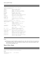
Retrieving the Current Time
There are two equivalent ways to retrieve the current value of the simulation clock. One is to call
the simtime function.
Prototype: double simtime (void)
Example: x = simtime ();
The other is to reference the variable clock.
Example: x = clock;
Delaying for an Amount of Time
A CSIM process can delay for a specified amount of simulation time by calling the hold function.
Prototype: void hold (double amount_of_time)
Example: hold (1.0);
If there are other processes waiting to run, the calling process will be suspended. Otherwise, time
will immediately advance by the specified amount.
Caution: It is a common mistake to call hold with the wrong type of parameter, such as an integer
value.
A process can delay until a specified time by calling hold with a parameter value equal to the
specified time minus the current time. To make a simulation begin with a clock value other than
zero, simply call hold at the beginning of the sim function with an amount of time equal to the
desired initial time.
Calling the hold function with a zero amount of time might at first seem to be meaningless. But, it
causes the running process to relinquish control to any other process that is waiting to run at the
same simulation time. This can be used to affect the order of execution of processes that have
activities scheduled for the same simulation time.
Advancing Time
There is no way for a program to directly assign a value to the simulation clock. The simulation
clock advances as a side effect of a process performing one of the following function calls.
hold allocate wait
queue use timed_allocate
wait_any queue_any reserve
receive timed_wait timed_queue
timed_reserve timed_receive
Calling one of these functions does not guarantee that time will advance. For example, calling the
allocate function will cause time to pass only if the requested amount of storage is not available.
All CSIM function calls other than those in the above list, as well as all C language statements,
occur instantaneously with respect to simulation time. A CSIM program can perform arbitrarily
many activities in a single instant of simulation time.
A common programming error is to create a CSIM process that calls none of the functions in the
above list. When this process receives control, it runs endlessly to the exclusion of all other CSIM
processes.
Displaying the Time
There are several ways the simulation time can be automatically displayed while running a CSIM
program. Every trace message contains the current simulation time. The variable clock and the
function simtime() can be used to get the current simulated time. Also, when the report function is
called to produce a report of all statistics, the report header contains the current simulation time.
Integer-Valued Simulation Time
In some simulation models, such as models of computer hardware, it is the case that time can only
assume discrete integer values. Although CSIM maintains time as a floating point variable, some
simple programming techniques can insure that the clock will always have an integer value. (Here,
we are using the word "integer" in the mathematical sense.)Amounts of time appear as input
parameters in calls to the following functions: hold, use, timed_reserve, timed_wait, timed_receive,
and timed_queue. To maintain an integer-valued clock, these parameters must have values that are
integers (although of type double). This can be accomplished either by specifying a floating point
numeric literal that has an integer value or by type casting an integer expression to type double.
Example: hold (10.0);
Example: use (bus, (double) uniform_int(1,5));
Example: use (bus, (double) floor (exponential(1.0)));
The IEEE Floating Point Standard guarantees that addition and subtraction with integer valued
operands will yield integer valued results. CSIM performs only addition on the simulation clock.
Processes
Processes represent the active entities in a CSIM model. For example, in a model of a bank,
customers might be modeled as processes (and tellers as facilities). In CSIM, a process is a C
procedure which executes a create statement. A CSIM process should not be confused with a UNIX
process (which is an entirely different thing). The create statement is similar to a UNIX "fork"
statement. A process can be invoked with input arguments, but it cannot return a value to the
invoking process.
There can be several simultaneously "active" instances of the same process. Each of these instances
appears to be executing in parallel (in simulated time) even though they are in fact executing
sequentially on a single processor. The CSIM runtime package guarantees that each instance of
every process has its own runtime environment. This environment includes local (automatic)
variables and input arguments. All processes have access to the global variables of a program.
A CSIM process, just like a real process, can be in one of four states:
Actively computing
Ready to begin computing
Holding (allowing simulated time to pass)
Waiting for an event to happen (or a facility to become available, etc.)
When an instance of a process terminates, either explicitly or via a procedure exit, it is deleted from
the CSIM system. Each process has a unique process id and each has a priority associated with it.
Initiating a Process
In CSIM, a process is a procedure which executes a create statement; a process is initiated
(invoked, started, ...) by executing a standard procedure call:
Prototype: void proc(arg1, ..., argn);
Example: my_proc(a, 64, "label");
In some cases, the process initiator requires the id of the initiated process. In these cases, the
prototype and example appear as follows:
Prototype: long proc(arg1, . . ., argn);
Example: proc_id = my_proc(a, 32, "label");
Caution: It is bad practice to pass the address of a local variable to a CSIM process as an input
argument.
Caution: A process cannot return a function value.
Caution: A create statement (see below) must appear in the initiated process.
Executing the Process CREATE Statement
As stated above, a CSIM process is a procedure which executes the create statement:
Prototype: void create (char* name)
Example: create ("customer");
The name of a process is just a character string which is used to identify the process in event traces
and reports generated by CSIM. Typically, the create statement is executed at the beginning of a
process. Each instance of a process is given a unique process id (process id’s are not reused).
Processes can invoke procedures and functions in any manner. Processes can also initiate other
processes.
When a procedure executes its create statement, the following actions take place:
The process executing the create statement (the called process) is established and is made
"ready to execute" at the statement following the create statement, and
The calling process continues its execution (i.e., it remains the actively computing process) at
the statement after the procedure call to the called process.
The calling process continues as the active process until it suspends itself.
No simulated time passes during the execution of a createstatement.
Process Operation
Processes appear to operate simultaneously with other active processes at the same points in
simulated time. The CSIM process manager creates this illusion by starting and suspending
processes as time advances and as events occur. Processes execute until they "’suspend" themselves
by doing one of the following actions:
execute a hold statement (delay for a specified interval of time),
execute a statement which causes the processes to be placed in a queue, or
terminate.
Processes are restarted when the time specified in a holdstatement elapses or when a delay in a
queue ends. It should be noted that simulated time passes only by the execution of hold statements.
While a process is actively computing, no simulated time passes.
The process manager preserves the correct context for each instance of every process. In particular,
separate versions of all local variables (variables resident in the runtime stack frame) and input
arguments for a process are maintained. CSIM accomplishes this by saving and restoring process
contexts (segments of the runtime stack) as processes suspend themselves and as processes are
"resumed" (restored). A consequence of this kind of operation is that if one processes passes an
address of a local variable to another process, it is likely that when this address is referenced, the
reference will be invalid. The reason is that when a process is not actually computing (using the real
CPU), its stack frame with the local variables will not be physically located in the correct place in
memory. This is not a major obstacle to writing efficient and useful models; it is a detail which
must be remembered as CSIM models are developed.
Terminating a Process
A process terminates when it either does a normal procedure exit or when it executes a terminate
statement.
Prototype: void terminate (void)
Example: terminate ();
The normal case is for a process to do a normal procedure exit or return. The terminate statement is
provided when this normal case is not appropriate.
Changing the Process Priority
The initial priority of a process is inherited from the initiator of that process. For the sim (main)
process, the default priority is 1 (low priority).
Prototype: void set_priority (long new_priority)
Example: set_priority (5);
This statement must appear after the create statement in a process. Lower values represent lower
priorities (i.e. priority 1 processes will run later than priority 2 processes when priority is a
consideration in order of execution (see section 4.10, "Changing the Service Discipline at a
Facility").
Inspector Functions
These functions each return some information to the process issuing the statement. The type of the
returned value for each of these functions is as indicated.
Prototype: Functional Value:
char* process_name (void)
retrieves pointer to name of process issuing inquiry
long identity (void)
retrieves the identifier (process number) of process issuing the inquiry
long priority (void)
retrieves the priority of process issuing inquiry
Reporting Process Status
To print the status of each active process in a model:
Prototype: void status_processes (void)
Example: status_processes ();
To print the status of processes with pending state changes (the "next event list"):
Prototype: void status_next_event_list (void)
Example: status_next_event_list ();
These reports will be written to the default output location or to that specified by set_output_file
(see section 19.7, "Output File Selection").
Facilities
A facility is normally used to model a resource (something a process requests service from) in a
simulated system. For example, in a model of a computer system, a CPU and a disk drive might
both be modeled by CSIM facilities. A simple facility consists of a single server and a single queue
(for processes waiting to gain access to the server). Only one process at a time can be using a
server. A multiserver-server facility contains a single queue and multiple servers. All of the waiting
processes are placed in the queue until one of the servers becomes available. A facility set is an
array of simple facilities; in essence, a facility set consists of multiple single server facilities, each
with its own queue.
Normally, processes are ordered in a facility queue by their priority (a higher priority process is
ahead of a lower priority process). In cases of ties in priorities, the order is first-come, first-served
(fcfs). An fcfs facility can be designated as a synchronous facility. Each synchronous facility has its
own clock with a period and a phase and all reserve operations are delayed until the onset of the
next clock cycle. Service disciplines other than priority order can be established for a server. These
are described in section 4.10, "Changing the Service Discipline at a Facility".
A set of usage and queueing statistics is automatically maintained for each facility in a model. The
statistics for all facilities which have been used are "printed" when either a report (see section 17.2,
"CSIM Report Output") or a report_facilities is executed (see section 4.4, "Producing Reports" for
details about the reports that are generated). In addition, there is a set of inspector functions that can
be used to extract individual statistics for each facility.
First time users of facilities should focus on the following four sections, which explain how to set
up facilities, use (and reserve and release) facilities, and produce reports. Subsequent sections
describe the more advanced features of facilities.
Declaring and Initializing a Facility
A facility is declared in a CSIM program using the built-in type FACILITY.
Example: FACILITY f;
Before a facility can be used, it must be initialized by calling the facility function.
Prototype: FACILITY facility (char* name)
Example: f = facility ("fac");
A newly created facility is created with a single server which is "free". The facility name is used
only to identify the facility in output reports and trace messages.
Facilities should be declared with global variables and initialized in the first process (normally the
process named sim) prior to the beginning of the simulation part of the model. Unless changed by a
set_servicefunc statement (see section 4.10, "Changing the Service Disciplines at a Facility"), the
scheduling policy of the facility will be first-come, first-served (fcfs).
Using a Facility
A process typically uses a server for a specified interval of time.
Prototype: void use (FACILITY f, double service_time)
Example: use (f, expntl(1.0));
If the server at this facility is free (not being used by another process), then the process gains
exclusive use of the server and the usage interval starts immediately. At the end of the usage
interval, the process gives use of the server and departs this facility. Execution continues at the
statement following the use statement.
If the server at this facility is busy (is being used by another process), then the newly arriving
process is placed in a queue of waiting processes; this queue is ordered by process priority, with
processes of equal priority being ordered by time of arrival. As each process completes its usage
interval, the process at the head of the queue is assigned to the server and its usage interval starts at
that time.
The service discipline at a facility specifies how processes are given access to the server. One of
several different service disciplines can be specified for a facility. Also, another form of facility has
multiple servers. In addition, it is possible to have an array of facilities (a facility set). The
difference between a multiserver facility and a facility set is that a multiserver facility has one
queue for all of the waiting processes, while a facility set has a separate queue for each facility in
the set.
Reserving and Releasing a Facility
In some cases, a process will acquire a server, but will do something other than enter the usage
interval when it gets the server. The statements for doing this are reserve (to gain exclusive use of a
server) and release (to relinquish use of the server acquired in a previous reserve statement)
Prototypes: long reserve (FACILITY f)
void release (FACILITY f)
Examples: reserve (f);
release(f);
When a process executes a reserve, it either gets use of the server immediately (if the server is not
busy) or it is suspended and placed in a queue of processes waiting to get use of the server. When it
gains access to the server, it executes the statement following the reserve statement. The order of
processes in the queue is by process priority, with processes of equal priority being ordered by time
of arrival. This process priority service discipline is called fcfs in CSIM; it (along with fcfs_sy, see
below) is the only service discipline that can be specified for facilities where processes do this
reserve-releasestyle of access. If another service discipline is in force, then the processes must
execute use statements instead of reserve-release pairs of statements.
The process releasing a server at a facility must be the same process as the one which reserved it. If
this is not the case, then the release_server statement (see below) must be used. When a process
executes a release, it gives up use of the server; if there is at least one process waiting to start using
the server (i.e., there is at least one process in the queue at this facility), the process at the head of
the queue is given access to the server and that process is then reactivated and will proceed by
executing the statement following its reserve statement. No simulation time passes during execution
of a release statement.
Note: Executing the sequence "reserve(f); hold(t); release(f);" is equivalent to executing the
statement "use(f,t);". However, if the usage interval is specified by a random number function, then
there is a subtle difference between these, as follows: the randomly derived interval is determined
after gaining access to the server in the first sequence and before gaining access to the server with
the use form; thus it is likely that the intervals in these two examples will be different. In other
words, the sequence "reserve(f); hold (exponential (t)); release(f);" will not necessarily display
exactly the same behavior as executing the statement "use(f,exponential (t));".
Producing Reports
Reports for facilities are most often produced by calling the report function which prints reports of
all the CSIM objects. Reports can be produced for all existing facilities by calling the
report_facilities function.
Prototype: void report_facilities ( void )
Example: report_facilities ();
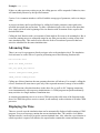
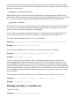
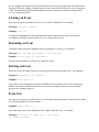
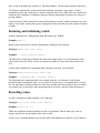
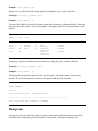
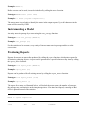
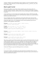
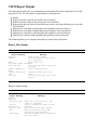
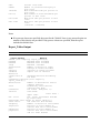
The report for a facility, as illustrated below, includes, for each facility, the name of the facility, the
service discipline, the average service time, the utilization, the throughput rate, the average queue
length, the average response time and the number of completed service requests.
FACILITY SUMMARY
facility service service through queue response compl
name disc time util. put length time count
f fcfs 0.40907 0.208 0.50900 0.27059 0.53162 509
ms fac fcfs 1.50020 0.764 0.50900 0.83821 1.64678 509
> server 0 1.55358 0.494 0.31800 318
> server 1 1.41133 0.270 0.19100 191
q rnd_rob 0.73437 0.507 0.69000 0.95522 1.38438 690
Releasing a Specific Server at a Facility
Sometimes, it is necessary for one process to reserve a facility and then for another process to
release the server obtained by the first process. In this case, the first process has to save the index of
the server it obtained, and then give this server index to the second process, so that it can specify
that index in the release_server statement, as follows:
Example: server_index = reserve ( f ) ;
Prototype: void release_server (FACILITY f, long server_index)
Example: release_server (f, server_index);
This operates in the same way as the release statement except that the ownership of the server is not
checked; thus, a process which did not reserve the facility may release it by executing the
release_server statement with a server index.
Declaring and Initializing a Multiserver Facility
In some cases, a facility has multiple servers, and each of these servers is indistinguishable from the
other servers. A mutliserver facility is declared as a normal (single server) facility.
Example: FACILITY cpu;
However, a multiserver facility is initialized in a different manner.
Prototype: FACILITY facility_ms ( char *name, long number_of_servers)
Example: cpu = facility_ms ( "dual cpu", 2);
A process can either execute a use statement or the reserve-release pair of statements at a
multiserver facility. In either case, the process gains access to any server that is free; a process is
suspended and put in the single queue at the facility only when all of the servers are busy.
Facility Sets
A facility set is an array of facilities.
Example: FACILITY disk[10]
A facility set is initialized as follows:
Prototype: void facility_set ( FACILITY f[],char *name, long num_facilities ) ;
Example: facility_set ( disk, "disk", 10 ) ;
In a facility set, each element of the set is an independent, single server facility, with its own queue.
Each of these facilities is given a constructed name which shows its position in the set. In the above
example, the name for the first element of the set is "disk[0]". Facility sets are used to model cases
where each server has its own queue of waiting processes.
Reserving a Facility with a Time-out
Sometimes a process must not wait indefinitely to gain access to a server. If a process executes the
timed_reserve function, it will be suspended until either it gains use of a server or the specified
time-out interval expires.
Prototype: long timed_reserve (FACILITY f, long timeout)
Example: result = timed_reserve (f, 100.0); if ( result ! = TIMED_OUT) . . .
The process must check the functional value, to determine whether or not it obtained a server. If the
value TIMED_OUT is returned, the process did not obtain a server. If this is not returned
(EVENT_OCCURRED will in fact be returned), then the process did obtain a server and should
eventually release the server.
Renaming a Facility
The name of a facility can be changed at any time, as follows:
Prototype: void set_name_facility (FACILITY f, char *new_name)
Example: set_name_facility (f, "cpus");
Only the first ten characters of the facility’s name are stored.
Changing the Service Discipline at a Facility
The service discipline for a facility determines the order in which processes at the facility are given
access to that facility. If not otherwise specified, the service discipline for a facility is fcfs. When
the priorities differ, processes gain access to the server in priority order (higher priority processes
before lower priority processes). When processes have the same priority, the processes gain access
in the order of their arrival at the facility (first come, first served). This default service discipline
can be changed.
Prototype: void set_servicefunc (FACILITY f, void(*service_function)())
Example: set_servicefunc (f, pre_res);
Set_servicefunc() refers to a service function which is invoked when the use statement (described
above) references this facility. This service function can be any of the following pre-defined service
discipline functions:
fcfs - first come, first served
This is the default service discipline and is described in the introduction to this section. If the
synchronous_facility statement (see below) is used for this facility, this will behave like a fcfs_sy
(clock synchronized fcfs) facility. In other words, there are two ways for a facility to become
synchronized: specifying the service discipline of fcfs_sy or specifying (or defaulting) fcfs for the
service discipline and using the synchronous_facility statement.
fcfs_sy - first come, first served, clock synchronized
This is the same as fcfs except that requests can be satisfied only at the beginning of a clock cycle.
If not otherwise specified (via synchronous_facility below), the clock phase (time to onset of first
clock cycle) will be 0.0, and the period (length of a clock cycle) will be 1.0.
inf_srv - infinite servers
There is no queueing delay at all since there is always a server available at the facility.
lcfs_pr - last come, first served, preempt
Arriving processes are always serviced immediately, preempting a process that is currently being
served if necessary. Priority is not a consideration with this service discipline.
prc_shr - processor sharing
This is load-dependent processor sharing. Service times for each process are determined based on
the number of processes at the facility. If not otherwise specified (see set_loaddep below), it will be
assumed that the rate that applies when there are n processes at the facility is n (in other words, if
there are n processes at the facility, the service time will be multiplied by n). The altered service
times are recomputed as tasks that arrive at and leave the facility. There is no queueing delay with
processor sharing since the assumption is that the server works faster and faster as necessary to
service all processes that request it.
There can be a maximum of 100 processes sharing a prc_shrfacility.
pre_res - preempt resume
Higher priority processes will preempt lower priority processes, so that the highest priority process
at the facility will always finish using it first. Where the priorities are the same, processes will be
served on a first come, first served basis. Preempted processes will eventually resume and complete
their service time interval.
rnd_pri - round robin with priority
Higher priority processes will be served first. When there are multiple processes with the same
priority, they will be serviced on a round robin basis, with each getting the amount of time specified
in set_timeslice (see below) before being preempted by the next process of the same priority.
rnd_rob - round robin
Processes will be serviced on a round robin basis, with each getting the amount of time specified in
set_timeslice (see below) before being preempted by the next process requiring service. Process
priority is not a consideration with this service discipline.
Caution: The use statement (as opposed to thereserve ) statement must be used for most of these
service disciplines to be effective. Only fcfs and fcfs_sy will operate properly with reserve.
To set the clock information for the fcfs_sy service discipline:
Prototype: void synchronous_facility (FACILITY f, double phase, double period)
Example: synchronous_facility (f, 0.0, 1.0);
To set the load dependent service rate for the prc_shr(see above) service discipline:
Prototype: void set_loaddep (FACILITY f, double rate[], long n)
Example: set_loaddep(f, rate, 10);
The "rate" array is an array of length n, where each element specifies the service rate for the
corresponding number of processes using the server. Rate[i] is the amount by which the service
time is multiplied when there are processes at the facility. If n is less than the 100 (the maximum
number of processes allowed to share use of a prc_shr facility), then the value of the last specified
rate is replicated until 100 values are available. Also, if n is greater than 99, only 100 values will be
used. It should be remembered that the altered service times are recomputed as tasks arrive at and
leave the facility.
To set the time slice for the round robin service disciplines, rnd_pri and rnd_rob (see above):
Prototype: void set_timeslice (FACILITY f, double slice_length)
Example: set_timeslice (f, 0.01);
Deleting a Facility or a Facility Set
To delete a facility:
Prototype: void delete_facility (FACILITY f)
Example: delete_facility (f);
To delete a facility set:
Prototype: void delete_facility_set (FACILITY if_set[])
Example: delete_facility_set (f_set);
Caution: Deleting a facility or facility set is an extreme action and should be done only when
necessary.
Collecting Class-Related Statistics
Information about usage of a facility by processes belonging to different process classes can be
collected for all facilities or for a specific facility. To collect class-based usage information for a
specific facility:
Prototype: void collect_class_facility (FACILITY f)
Example: collect_class_facility (f);
Usage of this facility by all process classes (see section 15, "Process Classes") will be reported in
the facilities report. Also, it is an error to change the maximum number of classes allowed after this
statement has been executed.
To collect usage information for all facilities:
Prototype: void collect_class_facility_all (void)
Example: collect_class_facility_all ();
This applies to all of the facilities in existence when this statement is executed Usage of the
facilities by all process classes (see section 15, "Process Classes" ) will be reported in the facilities
report. It is an error to change the maximum number of classes allowed after this statement has
been executed.
Inspector Functions
All statistics and information maintained by a facility can be retrieved during execution of a model
or upon its completion.
Prototype: Functional Value:
pointer to name of facility
char* facility_name (FACILITY f)
long num_servers (FACILITY f)
number of servers at facility
char* service_disp (FACILITY f)
double timeslice (FACILITY f)
pointer to name of service discipline at facility
time in each time-slice for facility (which has a round robin
service discipline)
long num_busy (FACILITY f)
long qlength (FACILITY f)
number of servers currently busy at facility
number of processes currently waiting at facility
current status of facility
Busy if all servers are in use
FREE if at least one server is not in use
long status (FACILITY f)
long completions (FACILITY f)
long preempts (FACILITY f)
number of completions at facility
number of preempted requests at facility
double qlen (FACILITY f)
mean queue length at facility
double resp (FACILITY f)
mean response time at facility
double serv (FACILITY f)
mean service time at facility
double tput (FACILITY f)
mean throughput rate at facility
double util (FACILITY f)
utilization (% of time busy) at facility
Additional data on servers and classes can be obtained as follows:
number of completions for server sn at
long server_completions (FACILITY f, long sn)
facility
double server_serv (FACILITY f, long sn)
mean service time for server sn at facility
double server_tput (FACILITY f, long sn)
mean throughput rate for server sn at facility
double server_util (FACILITY f, long sn)
utilization for server sn at facility
long class_completions (FACILITY f, CLASS c)
number of completions for class at facility
double class_qlen (FACILITY f, CLASS c)
mean queue length for class at facility
double class_resp (FACILITY f, CLASS c)
mean response time for class at facility
double class_serv (FACILITY f, CLASS c)
mean service time for class at facility
double class_tput (FACILITY f, CLASS c)
mean throughput rate for class at facility
double class_util (FACILITY f, CLASS c)
utilization for class at facility
Status Report
To obtain a report on the status of all of the facilities in a model:
Prototype: void status_facilities (void)
Example: status_facilities ();
This report lists each facility along with the number of servers, the number of servers which are
busy, the number of processes waiting. the name and id of each process at a server, and the name
and id of each process in the queue.
Storages
A CSIM storage is a resource which can be partially allocated to a requesting process. A storage
consists of a counter (to indicate the amount of available storage) and a queue for processes waiting
to receive their requested allocation. A storage set is an array of these basic storages.
A storage can be designated to be synchronous. In a synchronous storage, each allocate is delayed
until the onset of the next clock cycle.
Usage and queueing statistics are automatically maintained for each storage unit. These are
"printed" whenever a report or a report_storages statement is executed (see section 17.2, "CSIM
Report Output" for details about the reports that are generated).
Declaring and Initializing Storage
A storage is declared in a CSIM program using the built-in type STORE.
Example: STORE s;
Before a storage can be used, it must be initialized by calling the storage function.
Prototype: STORE storage (char* name, long size)
Example: s = storage ("memory", 1000);
A newly created storage is created with all of the "storage" available. Storages should be declared
with global variables in the sim (main) process, prior to the beginning of the simulation part of the
model. A storage must be initialized via the storage statement before it can be used in any other
statement.
Allocating from a Storage
The elements of a storage can be allocated to a requesting process.
Prototype: void allocate (long amount, STORE s)
Example: allocate (10, s);
The amount of storage requested is compared with the amount of storage available at s. If the
amount of available storage is sufficient, the amount available is decreased by the requested amount
and the requesting process continues. If the amount of available storage is not sufficient, the
requesting process is suspended. When some of the storage elements are deallocated by some other
process, the highest priority waiting processes are automatically allocated their requested storage
amounts (as they can be accommodated), and they are allowed to continue. The list of waiting
processes is searched in priority order until a request cannot be satisfied. In order to preserve
priority order, a new request which would fit but which would get in front of higher priority waiting
requests will be queued.
Caution: The order of the arguments for the allocate statement (and the deallocate statement too)
can be confusing. Think of "allocating n elements of storage from storage s ".
Deallocating from a Storage Unit
To return storage elements to a storage, the deallocate procedure is used.
Prototype: void deallocate (long amount, STORE s)
Example: deallocate (10, s);
If there are processes waiting, the highest priority processes that are waiting are examined. Those
that will now fit have their requests satisfied and are allowed to continue. If a deallocate operation
causes the count of the number of using processes to become negative, an error is detected and
execution stops. This occurs whenever more deallocates than allocates are done, regardless of the
storage amounts or the number of different processes involved. Executing a deallocate statement
causes no simulated time to pass.
Caution: There is no check to insure that a process returns only the amount of storage that it had
been previously allocated.
Caution: A runtime error is detected if the number of deallocates exceeds the number of allocates at
a storage.
Producing Reports
Reports for storages are most often produced by calling the report function, which reports for all
CSIM objects. Reports can be produced for all existing storages by calling the report_storages
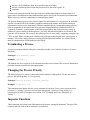
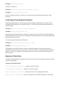
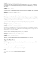
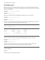
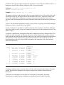
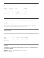
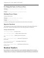
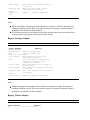
function. The report for a storage, as illustrated below, gives the name of the storage, the size
(initial amount), the average allocation request, the utilization, the average time each request is "in"
the storage, the average queue length, the average response time and the number of completed
requests.
STORAGE SUMMARY
storage alloc service queue response allocs
name size amount util. time length time compl
-----------------------------------------------------------------------------------------------------st 100 24.982 0.175 1.44064 0.72814 1.45338 501
Storage Sets
A storage set is an array of storages. Each element of the array is an individual storage.
Example: STORE *s_set, char *name [5];
A storage set must be initialized before the elements of the set can be used.
Prototype: void storage_set ( STORE* s_set. char
*name,long amount, long number_in_set);
Example: storage_set(s_set, "set", 100, 5);
The example initializes a set of five storages, each with 100 elements of storage available at the
onset of operation. The name is the name of the set. Each individual unit of storage is given a
unique (indexed) name. In the example, the first storage in the set is named "set[0]", the second is
named "set[1]", and so on. The last storage is named "set[99]". Similarly, the individual units of
storage are accessed as elements of an array. All of the operations which apply to a storage also
apply to the individual units of a storage set.
Allocating Storage with a Time-out
Sometimes, processes cannot wait indefinitely to allocate the needed amount of storage. If such a
process executes the timed_allocate function, then, if the requested amount of storage is not
available, the process will be suspended until either the requested amount of storage becomes
available or the time-out interval expires.
Prototype: long timed_allocate (long amount, STORE s,
double timeout)
Example: result = timed_allocate (10, s, 100.0);
if (result ! = TIMED_OUT) . . .
The process must check the function value (result) to determine whether or not the requested
storage was obtained. If the value TIME_OUT is returned, the process did not obtain any of the
requested storage. If this value is not returned (EVENT_OCCURRED will in fact be returned), then
the process did obtain the requested storage.
Making a Storage Unit Clock Synchronous
A storage unit can be designated to be a synchronous storage unit.
Prototype: void synchronous_storage (STORE s,
double.phase,double period)
Example: synchronous_storage (s, 0.0, 1.0);
A synchronous storage unit is similar to a normal storage unit except that allocation requests are
always delayed until the beginning of the next clock cycle. The clock phase specifies the interval
before the onset of the first clock cycle, and the period specifies the interval between successive
clock cycles.
Adding More Storage Elements to a Storage Unit
To increase the amount of storage (the number of storage elements) in a storage,
Prototype: void add_store (long amount, STORE s)
Example: add_store (100, s);
Renaming a Storage Unit:
The name of a storage can be changed at any time, as follows:
Prototype: void set_name_storage (STORE s, char
*new_name)
Example: set_name_storage (s, "cache");
Only the first ten characters of the storage’s name are stored.
Deleting Storage or a Storage Set
To delete a storage:
Prototype: void delete_storage (STORE s)
Example: delete_storage (s);
To delete a storage set:
Prototype: void delete_storage_set (STORE s_set[])
Example: delete_storage (s_set);
Deleting a storage or storage set is an extreme action and should be done only when necessary.
Inspector Functions
These functions each return a statistic which describes some aspect of the usage of the specified
storage.
Prototype: Functional Value:
pointer to name of store
char* storage_name(STORE s)
number of storages defined for
long storage_capacity(STORE s)
store
long avail (STORE s)
number of storages currently
available at store
number of processes currently
long storage_qlength(STORE s)
waiting at store
sum of requested amounts from
long storage_request_amt(STORE s)
store
time-weighted sum of
long storage_number_amt(STORE s)
requesters for store
busy time-weighted sum of
double storage_busy_amt(STORE s)
amounts for store
double storage_waiting_amt(STORE s)
waiting time weighted sum of
amounts for store
long storage_request_amt(STORE s)
total number of requests for
store
long storage_release_amt(STORE s)
total number of completed
requests for store
long storage_queue_cnt(STORE s)
number of queued requests at
store
double storage_time(STORE s)
time at store that is spanned by
report
Reporting Storage Status
Prototype: void status_storages (void)
Example: status_storages ();
The report will be written to the default output location or to that specified by set_output_file (see
section 19.7, "Output File Selection").
Events
Events are used to synchronize the operations of CSIM processes. An event exists in one of two
states: occurred or not occurred . A process can change the state of an event, or it can suspend its
execution until an event has occurred. When a process is suspended it can join a set of processes, all
of which will be resumed when the event occurs. Or, it can join an ordered queue from which only
one process is resumed for each occurrence of the event. An event is automatically reset to the not
occurred state when all of the suspended processes that can proceed have done so.
Advanced features of events include the ability to create sets of events for which processes can wait
and the ability for a process to bound its waiting time by specifying a time-out. Events can also be
used to construct other synchronization mechanisms such as semaphores.
Declaring and Initializing an Event
An event is declared in a CSIM program using the built-in type EVENT.
Example: EVENT e;
Before an event can be used, it must be initialized by calling the event function.
Prototype: EVENT event (char* name)
Example: e = event ("done");
An event is initialized in the not occurred state. The event name is used only to identify the event in
output reports and trace messages.
An event that is initialized in the first CSIM process (sim) exists during the entire simulation run
and is called a global event. An event initialized in any other process is called a local event. A local
event is deleted when the process in which it was initialized terminates. To make such an event
exist for the entire run, it must be initialized by calling the global_event function.
Prototype: EVENT global_event (char* name)
Example: e = global_event ("done");
Waiting for an Event to Occur
A process waits for an event to occur by calling the wait function.
Prototype: void wait (EVENT e)
Example: wait (e);
If the event is in the occurred state, control returns from the wait function immediately and the
event is changed to the not occurred state. If the event is in the not occurred state, the calling
process is suspended from further execution and control will not return from the wait function until
some other process sets this event. When the event is set, all waiting processes will be resumed and
the event will be placed in the not occurred state.
Waiting with a Time-Out
Sometimes a process must not be suspended indefinitely waiting for an event to occur. If a process
calls the timed_wait function, it will be suspended until either the event is set or the specified
amount of time has passed.
Prototype: long timed_wait (EVENT e, double timeout)
Example: result = timed_wait (e, 100.0);
if (result ! = TIMED_OUT)
The calling process should check the functional value to determine the circumstances under which
it was resumed. If the value EVENT_OCCURRED is returned, the process was activated because
the event has occurred; if the value TIMED_OUT is returned, the specified amount of time passed
without the event being set.
Queueing for an Event to Occur
A process joins the ordered queue for an event by calling the queue function.
Prototype: void queue (EVENT e)
Example: queue (e);
This function behaves similarly to the wait function, except that each time the event is set only one
queued process is resumed. The queue is maintained in order of process priority, with processes
having the same priority being ordered by time of insertion into the queue.
Queueing with a Time-out
If a process calls the timed_queue function, it will be suspended until either the event is set a
sufficient number of times for the process to be activated or the specified amount of time has
passed.
Prototype: long timed_queue (EVENT e, double timeout)
Example: result = timed_queue (e, 100.0);
if (result ! = TIMED_OUT) ...
The calling process should check the functional value to determine the circumstances under which
it was resumed. If the value EVENT_OCCURRED is returned, the process was activated because
the event occurred; if the value TIMED_OUT is returned, the specified amount of time passed
without the process being activated by the event being set.
Setting an Event
A process can put an event into the occurred state by calling the set function.
Prototype: void set (EVENT e)
Example: set (e);
Calling this function causes all waiting processes and one queued process to be resumed. If there
are no waiting or queued processes, the event will be in the occurred state upon return from the set
function. If there are waiting or queued processes, the event will be in the not occurred state upon
return. No simulation time passes during these activities. Setting an event that is already in the
occurred state has no effect.
Clearing an Event
A process can put an event into the not occurred state by calling the clear function.
Prototype: void clear (EVENT e)
Example: clear (e);
Clearing an event happens in zero simulation time and no processes are in any way affected.
Clearing an event that is already in the not occurred state has no effect.
Renaming an Event
The name of an event can be changed at any time using the set_name_event function.
Prototype: void set_name_event (EVENT e, char *new_name)
Example: set_name_event (e, "finished");
Only the first ten characters of the event’s name are stored.
Deleting an Event
When an event is no longer needed, its storage can be reclaimed using the delete_event function.
Prototype: void delete_event (EVENT e)
Example: delete_event (e);
If an event is local, only the process that created the event can delete it. Once an event has been
deleted, it must not be further referenced. It is an error to attempt to delete an event on which
processes are waiting or queued.
Event Sets
An event set is an array of related events for which some special operations are provided. An event
set is declared using the C array construct.
Example: EVENT e_set[10];
All events in an event set are initialized with a single call to the event_set function.
Prototype: void event_set (EVENT e_set[], char *name,
long number_of_events)
Example: event_set (e_set, "events", 10);
As with any C array, the events in an event set are indexed from 0 to num_events - 1. Individual
events in the event set can be manipulated using any of normal event functions (e.g. ., set, clear,
wait, queue).
Example: set (e_set[3]);
A process can wait for the occurrence of any event in an event set by calling the wait_any function.
Prototype: long wait_any (EVENT e_set[])
Example: event_index = wait_any (e_set);
This function returns the index of the event that caused the calling process to proceed. If multiple
events in the set are in the occurred state, the lowest numbered event is the one recognized by the
calling process. All processes that have called wait_any are activated by the next event that occurs,
and these processes all receive the same index value.
A process can join an ordered queue for an event set by calling the queue_any function.
Prototype: long queue_any (EVENT e_set[])
Example: event_index = queue_any (e_set);
Each time any event in the event set occurs, one process in the queue is activated. The functional
value is the same as that of the wait_any function. It is not currently possible to specify a time-out
for the wait_any or queue_any functions.
An entire event set is deleted by calling the delete_event_set function.
Prototype: void delete_event_set (EVENT e_set[])
Example: delete_event_set (e_set);
The delete_event function must not be called on individual members of an event set.
Inspector Functions
The following functions return information about the specified event at the time they are called.
Prototype: Functional value:
char* event_name (EVENT e)
pointer to name of event
number of processes waiting for
long wait_cnt (EVENT e)
event
long queue_cnt (EVENT e)
event
number of processes queued of
long event_qlen (EVENT e)
long state (EVENT e)
sum of wait_cnt and queue_cnt
state of event:
OCC if occurred or
NOT_OCC if not occurred
Status Report
The status_events function prints a report of the status of all events in the model.
Prototype: void status_events (void)
Example: status_events ();
For each event, the report includes its state, the number of processes waiting for it, the number of
processes queued for it, the name and id of all waiting processes, and the name and id of all queued
processes. The report is written to the default output stream or the stream specified in the last call to
set_output_file .
Built-In Events
A process can suspend itself until there are no other active processes by waiting on the built-in
event event_list_empty.
Example: wait (event_list_empty);
This event is automatically set by CSIM when all processes have terminated or are waiting for
something (e.g., a facility or storage). Modelers sometimes use this to force the initial (sim) process
to wait until all work in the system being modeled has completed. Upon being reactivated, the
initial process might then produce reports.
If run length control is involved for a table, qtable, meter or box, (see 14.3), a process can suspend
itself until the run length control mechanism signals the end of a run. This is done by waiting for
the built-in event converged.
Example: wait (converged);
Mailboxes
A mailbox allows for the synchronous exchange of data between CSIM processes. Any process
may send a message to any mailbox, and any process may attempt to receive a message from any
mailbox.
A mailbox is comprised of two FIFO queues: a queue of unreceived messages and a queue of
waiting processes. At least one of the queues will be empty at any time. When a process sends a
message, the message is given to a waiting process (if one exists) or it is placed in the message
queue. When a process attempts to receive a message, it is either given a message from the message
queue (if one exists) or it is added to the queue of waiting processes.
A message can be either a single long integer or a pointer to some other data object. If a process
sends a pointer, it is the responsibility of that process to maintain the integrity of the referenced data
until it is received and processed.
Declaring and Initializing a Mailbox
A mailbox is declared in a CSIM program using the built-in type MBOX.
Example: MBOX m;
Before a mailbox can be used, it must be initialized by calling the mailbox function.
Prototype: MBOX mailbox (char* name)
Example: m = mailbox ("requests");
A newly created mailbox contains no messages. The mailbox name is used only to identify the
mailbox in output reports and trace messages.
A mailbox that is initialized in the first CSIM process (sim) exists during the entire simulation run
and is called a global mailbox. A mailbox initialized in any other process is called a local mailbox.
A local mailbox is deleted when the process in which it was initialized terminates.
Sending a Message
A process sends a message by calling the send function.
Prototype: void send (MBOX m, long message)
Example: send (m, (long) buffer);
If one or more processes are waiting on this mailbox, the process at the head of the process queue
will resume execution and will be given this message. If no processes are waiting, this message will
be appended to the tail of the message queue. No simulation time passes during this function call.
Receiving a Message
A process receives a message by calling the receive function.
Prototype: void receive (MBOX m, long* message)
Example: receive (m,(long*) &ptr);
If one or more messages are queued at this mailbox, the calling process is given the message at the
head of the queue and continues executing. If no messages are queued, the process is suspended
from further execution and is added to the tail of the process queue for this mailbox.
Receiving a Message with a Time-out
Sometimes a process must not wait indefinitely to receive a message. If a process calls the
timed_receive function, it will be suspended until either a message is received or the specified
amount of time has passed.
Prototype: long timed_receive (MBOX m, long* message,
double timeout)
Example: result = timed_receive(m,(long*) &ptr, 100.0);
if (result ! = TIMED_OUT) ...
The calling process can check the functional value to determine the circumstances under which it
was resumed. If the value EVENT_OCCURRED is returned, the process was activated because a
message was received; if the value TIMED_OUT is returned, the specified amount of time passed
without the process being activated by the receipt of a message.
Renaming a Mailbox
The name of a mailbox can be changed at any time using the set_name_mailbox function.
Prototype: void set_name_mailbox (MBOX m, char *new_name)
Example: set_name_mailbox (m, "responses");
Only the first ten characters of the mailbox’s name are stored.
Deleting a Mailbox
When a mailbox is no longer needed, its storage can be reclaimed using the delete_mailbox
function.
Prototype: void delete_mailbox (MBOX m)
Example: delete_mailbox (m);
If a mailbox is local, only the process that created the mailbox can delete it. Once a mailbox has
been deleted, it must not be further referenced. Deleting a mailbox causes any unreceived messages
to be lost. It is an error to attempt to delete a mailbox on which processes are waiting.
Inspector Functions
The following functions return information about the specified mailbox at the time they are called.
Prototype: Functional value:
char* mailbox_name (MBOX m)
pointer to name of mailbox
if positive, number of unreceived messages; if negative, magnitude is
number of waiting processes
long msg_cnt (MBOX m)
Status Report
The status_mailboxes function prints a report of the status of all mailboxes in the model.
Prototype: void status_mailboxes (void)
Example: status_mailboxes ();
For each mailbox, the report includes the number of unreceived messages, the number of waiting
processes, and the name and id of all waiting processes. The report is written to the default output
stream or the stream specified in the last call to set_output_file.
Introduction to Statistics Gathering
CSIM automatically gathers and reports performance statistics for certain types of model
components, including facilities and storages. CSIM also provides four general-purpose statistics
gathering tools: tables, qtables , meters, and boxes. These tools can be used for the following
purposes:
to obtain statistics other than mean values for facilities and storages
to obtain statistics for other model components, such as mailboxes and events
to obtain statistics for selected submodels or for the model considered as a whole
to employ the run length control algorithms provided with CSIM (see section 14.3, "Run
Length Control")
Any statistics can of course be gathered by declaring and updating variables in a CSIM program.
But, the statistics gathering tools are powerful and comprehensive, and their use will decrease the
likelihood of programming errors that lead to incorrect statistics. Formatted reports of the statistics
gathered with these tools can easily be included in the model output.
The following steps are suggested for adding statistics gathering to a model:
Identify what statistics are of interest and which statistics gathering tools are appropriate.
Declare a global pointer (variable) for each statistics gathering tool that will be used.
Initialize each statistics gathering tool, usually at the beginning of the sim function.
Add instrumentation (i.e., function calls) to the model to feed data to the tools.
Generate reports by calling the report function.
The magnitudes of the performance statistics obviously depend on the time unit that is chosen for
the model. Most of the reports produced by the statistics gathering tools will accommodate floating
point numbers with six digits to the left of the decimal point and six digits to the right of the
decimal point. Up to nine digits can be displayed for integer values. The time unit should be chosen
to avoid performance values so far from unity that digits of interest are not displayed.
Tables
A table is used to gather statistics on a sequence of discrete values such as interarrival times,
service times, or response times. Data values are "recorded" in a table to include them in the
statistics. A table does not actually store the recorded values; it simply updates the statistics each
time a value is included. (See section 9.6, "Moving Windows", for the only exception to this rule.)
The statistics maintained by a table include the minimum, maximum, range, mean, variance,
standard deviation, and coefficient of variation. Optional features for a table allow the creation of a
histogram, the calculation of confidence intervals, and the computation of statistics for values in a
moving window.
First-time users of tables should focus on the following three sections, which explain how to set up
tables, record values, and produce reports. Subsequent sections describe the more advanced features
of tables.
Declaring and initializing a table
A table is declared in a CSIM program using the built-in type TABLE.
Example: TABLE t;
Before a table can be used, it must be initialized by calling the table function.
Prototype: TABLE table (char* name);
Example: t = table ("response times");
The table name is used only to identify the table in the output reports. Up to 80 characters in the
name will be stored by CSIM. A newly created table contains no values and all the statistics are
zero.
A table can be initialized as a permanent table using the permanent_table function.
Prototype: TABLE permanent_table (char* name)
Example: t = permanent_table ("response times");
The information in a permanent table is not cleared when the reset function is called, and a
permanent table is not deleted when rerun is called. In all other ways, a permanent table is exactly
like any other table. Permanent tables are often used to gather data across multiple runs of a model.
As a general rule, do not make a table permanent unless you have a specific reason for doing so.
Recording values
A value is included in a table using the record function.
Prototype: void record (double value, TABLE t)
Example: record (1.0, t);
Tables are designed to maintain statistics on data of type double. Data of other types, such as
integer, must be cast to type double in the call to record.
Caution: It is a common mistake to reverse the order of the parameters in calls to record. Think of
"recording the value x in table t".
Producing reports
Reports for tables are most often produced by calling the report function, which prints reports for
all statistics gathering objects. A report can be generated for a specified table at any time by calling
the report_table function.
Prototype: void report_table (TABLE t)
Example: report_table (t);
Reports can be produced for all existing tables by calling the report_tables function.
Prototype: void report_tables (void)
Example: report_tables ();
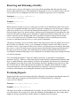
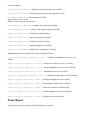
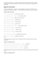
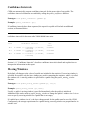
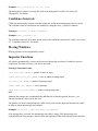
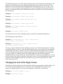
The report for a table will include the table name and all statistics, as illustrated below. If the table
is empty, a message to that effect is printed instead of the statistics.
TABLE 1: response times
minimum
maximum
range
0.009880
13.702809
13.692929
observations
mean
variance
standard
deviation
962
coefficient
of var
2.881970
7.002668
2.646255
0.918211
A summary report for all tables can be generated by calling the table_summary function.
Prototype: void table_summary (void)
Example: table_summary ();
The report that is produced contains one line for each table and includes only a subset of the
statistics. If a table is empty, no statistics will appear in the last three columns.
TABLE SUMMARY
standard
name observations mean maximum deviation
-----------------------------------------------------------------------------------------------------------------response times 962 2.881970 13.702809 2.646255
Histograms
A histogram can be specified for a table in order to obtain more detailed information about the
recorded values. The mode and other percentiles can often be estimated from a histogram. A
histogram is specified for a table by calling the table_histogram function.
Prototype: void table_histogram (TABLE t, long nbucket,
double min, double max)
Example: table_histogram (t, 10, 0.0, 10.0);
The number of buckets in the histogram will be nbucket. The smallest value in the first bucket will
be min; the largest value in the last bucket will be max. All buckets will have the same width of
(max-min)/nbucket. An underflow bucket and an overflow bucket will automatically be created if
needed to hold values less than min or greater than max.
Usually, a histogram is specified for a table immediately after the table is initialized. Additional
calls can be made to table_histogram to change the characteristics of the histogram, but only if the
table is empty.
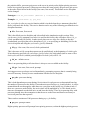
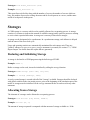
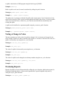
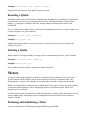
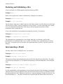
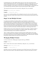
A report for a table having a histogram will include an additional section as illustrated below. For
each bucket in the histogram, the following information will be displayed: the smallest value the
bucket can hold, the number of values in the bucket, the proportion of all values that are in the
bucket, the proportion of all values in the bucket and all preceding buckets, and a bar whose length
corresponds to the proportion of values in the bucket.
lower frequency proportion
limit
0.00000
265
0.275468
1.00000
219
0.227651
2.00000
3.00000
4.00000
5.00000
6.00000
7.00000
8.00000
9.00000
>=10.00000
125
92
74
54
53
38
8
8
26
0.129938
0.095634
0.076923
0.056133
0.055094
0.039501
0.008316
0.008316
0.027027
cumulative
proportion
0.275468
********************
0.503119
*****************
0.633056 *********
0.728690 *******
0.805613 ******
0.861746 ****
0.916840 ****
0.956341 ***
0.964657 *
0.972973 *
1.000000 **
If leading or trailing buckets contain no values, the lines in the report for these buckets will not be
printed. This allows the histogram to be output as compactly as possible without losing any
information.
CSIM must save information for each bucket in a histogram. Consequently, the storage
requirements for a table that has a histogram are proportional to the number of buckets.
Confidence Intervals
CSIM can automatically compute confidence intervals for the mean of the data in any table. The
confidence interval calculations are enabled by calling the table_confidence function.
Prototype: void table_confidence (TABLE t)
Example: table_confidence (t);
If confidence intervals have been requested, the report for a table will have an additional section, as
illustrated below.
confidence intervals for the mean after 50000 observations
level
90 %
95 %
98 %
confidence interval
4.114119 +/- 0.296434 =
[3.817684, 4.410553]
4.114119 +/- 0.354041 =
[3.760078, 4.468159]
4.114119 +/- 0.421555 =
[3.692563, 4.535674]
rel. error
0.077648
0.078837
0.080279
Chapter 14, "Confidence Intervals and Run Length Control" describes confidence intervals in detail
and explains how to interpret the information in this report.
Moving Windows
By default, all values recorded in a table are included in the statistics. If a moving window is
specified for a table, only the last n values are used in computing the statistics, where n is called the
window size. A moving window is specified for a table using the table_moving_window function.
Prototype: void table_moving_window (TABLE t, long n)
Example: table_moving_window (t, 1000);
Usually, a table’s moving window is specified immediately after the table is initialized. Additional
calls can be made to table_moving_window to change the table’s window size. It is an error to
specify a moving window for a table that is not empty.
If a table has a window size of n, the last n values recorded in the table must be saved by CSIM.
Consequently, the storage requirements for a table having a moving window are proportional to its
window size.
Inspector Functions
All statistics maintained by a table can be retrieved during the execution of a model or upon its
completion. The attributes of a table (i.e., its name and moving window size) can also be retrieved.
Prototype: Functional value:
char* table_name (TABLE t)
pointer to name of table
long table_window_size (TABLE t)
long table_cnt (TABLE t)
size of moving window
number of values recorded
double table_min (TABLE t)
minimum value
double table_max (TABLE t)
maximum value
double table_sum (TABLE t)
sum of values
double table_sum_square (TABLE t)
double table_mean (TABLE t)
mean of values
double table_range (TABLE t)
double table_var (TABLE t)
range of values
variance of values
double table_stddev (TABLE t)
double table_cv (TABLE t)
sum of squares of values
standard deviation of values
coefficient of variation of
values
The following inspector functions retrieve information about the confidence interval associated
with a table:
Prototype: Functional Value:
double table_conf_halfwidth (double level, TABLE t)
halfwidth
double table_conf_lower (double level, TABLE t)
lower end
double table_conf_upper (double level, TABLE t)
upper end
The following inspector functions retrieve information about the run length control associated with
a table:
Prototype: Functional Value:
long table_batch_size (TABLE t)
current size of batch
long table_batch_count (TABLE t)
long table_converged (TABLE t)
number of batches used
TRUE or FALSE
double table_conf_mean (TABLE t)
mid point of conf. int.
double table_conf_accuracy (double level, TABLE t)
accuracy achieved
Although most statistics are mathematically undefined if there is no data, the corresponding
inspector functions return a value of zero if the table is empty.
The following inspector functions retrieve information about the histogram associated with a table.
Prototype: Functional value:
long table_histogram_num (TABLE t)
number of buckets
smallest value that is not
double table_histogram_low (TABLE t)
underflow
largest value that is not
double table_histogram_high (TABLE t)
overflow
double table_histogram_width (TABLE t)
width of each bucket
long table_histogram_bucket (TABLE t,long i)
number of values in
bucket
long taable_histogram_total(TABLE t)
number of values in all
buckets
The number of buckets in a histogram does not include the underflow or overflow buckets. Bucket
number 0 is the underflow bucket; bucket number 1+table_histogram_num( ) is the overflow
bucket. If a histogram has not been specified for a table, the above inspector functions all return
zero values.
The inspector functions that retrieve information about the results of run-length control are
described in section 14.3.
Renaming a Table
The name of a table can be changed at any time using the set_name_table function.
Prototype: void set_name_table (TABLE t, char* new_name)
Example: set_name_table (t, "elapsed time");
Only the first 80 characters of the table’s name are stored.
Resetting a Table
Resetting a table causes all information maintained by the table to be reinitialized. All optional
features selected for the table (e.g., histogram, confidence intervals, moving window) remain in
effect and are also reinitialized.
The reset function is usually used to reset all statistics gathering tools at once. A specific table can
be reset using the reset_table function.
Prototype: void reset_table (TABLE t)
Example: reset_table (t);
Although permanent tables are not reset by the reset function, they can be reset explicitly by calling
reset_table.
Deleting a Table
When a table is no longer needed, its storage can be reclaimed using the delete_table function.
Prototype: void delete_table (TABLE t)
Example: delete_table (t);
Once a table has been deleted, it must not be further referenced. If enhancements (either histogram,
confidence intervals, or moving window) have been defined for a table, the each of these
enhancements is also deleted when the corresponding table is deleted.
Qtables
A qtable is used to gather statistics on an integer-valued function of time, such as the length of a
queue, the population of a subsystem, or the number of available resources. Every change in the
value of the function must be "noted" by calling a CSIM function. A qtable does not actually save
the functional values; it simply updates the statistics each time the value changes. (See section 10.6
for the only exception to this rule.)
The statistics maintained by a qtable include the minimum, maximum, range, mean, variance,
standard deviation, and coefficient of variation. The number of changes in the functional value is
maintained, as well as the initial and final values. Optional features for a qtable allow the creation
of a histogram, the calculation of confidence intervals, and the computation of statistics for values
in a moving window.
First-time users of qtables should focus on the following three sections, which explain how to set up
qtables, note changes in their values, and produce reports. Subsequent sections describe the more
advanced features of qtables.
Declaring and Initializing a Qtable
A qtable is declared in a CSIM program using the built-in type QTABLE.
Example: QTABLE qt;
Before a qtable can be used, it must be initialized by calling the qtable function.
Prototype: QTABLE qtable (char* name)
Example: qt = qtable ("queue length");
The qtable name is used only to identify the qtable in the output reports. Up to 80 characters in the
name will be stored by CSIM. A newly created qtable has an initial value of zero. To create a qtable
with a non-zero initial value, call the note_state function (described below) immediately after
creating the qtable.
A qtable can be initialized as a permanent qtable using the permanent_qtable function.
Prototype: QTABLE permanent_qtable (char* name)
Example: qt = permanent-qtable ("queue length");
Noting a Change in Value
The most common way for the value of a qtable to change is for it to increase or decrease by one.
Such a change would occur when a customer joins a queue or a resource is allocated. The value of a
qtable is increased by one using the note_entry function.
Prototype: void note_entry (QTABLE qt)
Example: note_entry (qt);
The value of a qtable is decreased by one using the note_exit function.
Prototype: void note_exit (QTABLE qt)
Example: note_exit (qt);
The value of a qtable can be changed to an arbitrary number using the note_value function.
Prototype: void note_value (QTABLE qt, long value)
Example: note_value (qt, 12);
Producing Reports
Reports for qtables are most often produced by calling the report function, which prints reports for
all statistics gathering objects. A report can be generated for a specified qtable at any time by
calling the report_qtable function.
Prototype: void report_qtable (QTABLE qt)
Example: report_qtable (qt);
Reports can be produced for all existing qtables by calling the report_qtables function.
Prototype: void report_qtables (void)
Example: report_qtables ();
The report for a qtable will include the qtable name and all statistics, as illustrated below. If no time
has passed since the creation or reset of the qtable, a message to that effect is printed instead of the
statistics.
QTABLE 1: queue length
initial
final
entries
0
4
966
exits
962
minimum
maximum
range
0
14
14
mean
variance
standard
deviation
coeff of
variation
2.788416
8.529951
2.920608
1.047408
A summary report for all qtables can be generated by calling the qtable_summary function.
Prototype: void qtable_summary (void)
Example: qtable_summary ();
The report that is produced contains one line for each qtable and includes only a subset of the
statistics. If no time has passed, no statistics will appear in the last three columns.
QTABLE SUMMARY
standard
name entries exits mean maximum deviation
------------------------------------------------------------queue length 966 962 2.788416 14 2.920608
Histograms
A histogram can be specified for a qtable in order to obtain more detailed information about the
functional values. Depending on how the qtable is being used, its histogram might give the
distribution of the queue lengths, the subsystem population, or the number of available resources. A
histogram is specified for a table by calling the qtable_histogram function.
Prototype: void qtable_histogram (QTABLE qt, long
nbucket, long min, long max)
Example: qtable_histogram (qt, 11, 0, 10);
The number of buckets in the histogram will be (no greater than) nbucket. The smallest value in the
first bucket will be min; the largest value in the last bucket will be max. All buckets will have the
same width, which will be rounded up to an integer if necessary. An underflow bucket and an
overflow bucket will automatically be created if needed to hold values less than min or greater than
max.
Caution: The min and max parameters of qtable_histogram are of type long, whereas the analogous
parameters of table_histogram are of type double.
Usually, a histogram is specified for a qtable immediately after the qtable is initialized. Additional
calls can be made to qtable_histogram to change the characteristics of the histogram, but only if the
qtable is empty.
A report for a qtable having a histogram will include an additional section as illustrated below. For
each bucket in the histogram, the following information will be displayed: the smallest value the
bucket can hold, the total time the functional value was in the bucket, the proportion of time that the
functional value was in the bucket, the proportion of all functional values in the bucket and all
preceding buckets, and a bar whose length corresponds to the proportion of time the functional
value was in the bucket.
number
0
total time
248.74145
proportion
0.249003
1
185.45534
0.185651
2
157.13503
0.157300
3
4
5
6
7
8
9
10
100.01937
78.14196
62.59210
44.38455
35.33308
25.94494
21.48465
39.71625
0.100125
0.078224
0.062658
0.044431
0.035370
0.025972
0.021507
0.039758
>=
cumulative
proportion
0.249003
********************
0.434654
***************
0.591954
*************
0.692079
********
0.770303
******
0.832961
*****
0.877392
****
0.912762
***
0.938735
**
0.960242
**
1.000000
***
If leading or trailing buckets contain no values, the lines in the report for these buckets will not be
printed. This allows the histogram to be output as compactly as possible without losing any
information.
CSIM must save information for each bucket in a histogram. Consequently, the storage
requirements for a qtable that has a histogram are proportional to the number of buckets.
Confidence Intervals
CSIM can automatically compute confidence intervals for the mean value of any qtable. The
confidence interval calculations are enabled by calling the qtable_confidence function.
Prototype: void qtable_confidence (QTABLE qt)
Example: qtable_confidence (qt);
If confidence intervals have been requested, the report for a qtable will include an additional
section, as illustrated below.
confidence intervals for the mean after 29600.000000 time units
level
confidence interval
90 %
4.319412 +/- 0.491696 = [3.827715,
4.811108]
4.319412 +/- 0.588209 = [3.731203,
4.907621]
4.319412 +/- 0.701971 = [3.617441,
5.021382]
95 %
98 %
rel.
error
0.128457
0.157646
0.194052
Section 14.1, "Confidence Intervals", describes confidence intervals in detail and explains how to
interpret the information in this report.
Moving Windows
By default, all changes to the value of a qtable are included in the statistics. If a moving window is
specified for a qtable, only the last n changes are used in computing the statistics, where n is called
the window size. A moving window is specified for a qtable using the qtable_moving_window
function.
Prototype: void qtable_moving_window (QTABLE qt, long n)
Example: qtable_moving_window (qt, 1000);
Usually, a qtable’s moving window is specified immediately after the qtable is initialized.
Additional calls can be made to qtable_moving_window to change the qtable’s window size. It is an
error to specify a moving window for a qtable that is not empty.
If a qtable has a window size of n, the last n changes noted for the qtable must be saved by CSIM.
Consequently, the storage requirements for a qtable having a moving window are proportional to its
window size.
Note: In an alternate implementation of moving windows, the window size would be specified as an
amount of time. The storage requirements of such an implementation would be non-constant and
potentially prohibitive.
Inspector Functions
All statistics maintained by a qtable can be retrieved during the execution of a model or upon its
completion. The attributes of a qtable (i.e., its name and moving window size) can also be retrieved.
Prototype: Functional value:
char* qtable_name (QTABLE qt)
pointer to name of qtable
moving window size
long qtable_window_size (QTABLE qt)
long qtable_entries (QTABLE qt)
number of note_entry’s
number of note_exit’s
long qtable_exits (QTABLE qt)
long qtable_min (QTABLE qt)
minimum value
long qtable_max (QTABLE qt)
maximum value
long qtable_initial (QTABLE qt)
initial value
long qtable_current (QTABLE qt)
current value
double qtable_sum (QTABLE qt)
sum of values weighted by time
double qtable_sum_square (QTABLE qt)
sum of squared weighted
mean value
double qtable_mean (QTABLE qt)
long qtable_range (QTABLE qt)
range of values
double qtable_var (QTABLE qt)
variance of values
double qtable_stddev (QTABLE qt)
double qtable_cv (QTABLE qt)
standard deviation of values
coefficient of variation of values
The following inspector functions retrieve information about the confidence interval associated
with a table:
Prototype: Functional Value:
double qtable_conf_halfwidth (double level, QTABLE qt)halfwidth
double qtable_conf_lower (double level, QTABLE qt)
lower end
double qtable_conf_upper (double level, QTABLE qt)
upper end
The following inspector functions retrieve information about the run length control associated with
a table:
Prototype: Functional Value:
long qtable_batch_size (QTABLE qt)
current size of batch
long qtable_batch_count (QTABLE qt)
number of batches used
double qtable_conf_mean (QTABLE qt)
mid point of conf. int.
long qtable_converged (QTABLE qt)
TRUE or FALSE
double qtable_conf_aaccuracy (double level, QTABLE qt)accuracy
achieved
Many statistics are mathematically undefined if zero time has passed since the creation or reset of a
qtable. The corresponding inspector functions return a value of zero in this case.
The following inspector functions retrieve information about the histogram associated with a qtable.
Prototype: Functional value:
long qtable_histogram_num (QTABLE qt)
number of buckets
double qtable_histogram_low (QTABLE qt)
smallest value that is
not underflow
double qtable_histogram_high (QTABLE qt)
largest value that is not
overflow
double qtable_histogram_width(QTABLE qt)
width of each bucket
long qtable_histogram_bucket (QTABLE qt,long i)
total time value is in
bucket
The number of buckets in a histogram does not include the underflow or overflow buckets. Bucket
number 0 is the underflow bucket; bucket number 1+qtable_histogram_num( ) is the overflow
bucket. If a histogram has not been specified for a qtable, the above inspector functions all return
zero values.
The inspector functions that retrieve information about the results of run-length control are
described in section 14.3, "Run Length Control".
Renaming a Qtable
The name of a qtable can be changed at any time using the set_name_qtable function.
Prototype: void set_name_qtable (QTABLE qt, char
*new_name)
Example: set_name_qtable (qt, "number in queue");
Only the first 80 characters of the qtable’s name are stored.
Resetting a Qtable
Resetting a qtable causes all information maintained by the qtable to be reinitialized, except that the
current value is saved for use in computing future values. All optional features selected for the
qtable (e.g., histogram, confidence intervals, moving window) remain in effect and are also
reinitialized.
The reset function is usually used to reset all statistics gathering tools at once. A specific qtable can
be reset using the reset_qtable function.
Prototype: void reset_qtable (QTABLE qt)
Example: reset_qtable (qt);
Although permanent qtables are not reset by the reset function, they can be reset explicitly by
calling reset_qtable.
Deleting a Qtable
When a qtable is no longer needed, its storage can be reclaimed using the delete_qtable function.
Prototype: void delete_qtable (QTABLE qt)
Example: delete_qtable (qt);
Once a qtable has been deleted, it must not be further referenced.
Meters
A meter is used to gather statistics on the flow of entities such as customers or resources past a
specific point in a model. Meters can be used to measure arrival rates, completion rates, and
allocation rates. A meter can be thought of as a probe that is inserted at some point in a model.
While a meter primarily measures the rate at which entities flow past it, a meter also keeps statistics
on the times between passages. These interpassage times are recorded in a table, which is an
integral part of every meter.
First-time users of meters should focus on the following three sections, which explain how to set up
meters, update meters, and produce reports. Subsequent sections describe the more advanced
features of meters.
Declaring and Initializing a Meter
A meter is declared in a CSIM program using the built-in type METER.
Example: METER m;
Before a meter can be used, it must be initialized by calling the meter function.
Prototype: METER meter (char* name)
Example: m = meter ("system completions");
The meter name is used only to identify the meter in the output reports. Up to 80 characters in the
name will be stored by CSIM.
Instrumenting a Model
An entity notes its passage by a meter using the note_passage function.
Prototype: void note_passage (METER m)
Example: note_passage (m);
For the statistics to be accurate, every entity of interest must note its passage and do so at the
correct time.
Producing Reports
Reports for meters are most often produced by calling the report function, which prints reports for
all statistics gathering objects. A report can be generated for a specified meter at any time by calling
the report_meter function.
Prototype: void report_meter (METER m)
Example: report_meter (m);
Reports can be produced for all existing meters by calling the report_meters function.
Prototype: void report_meters (void)
Example: report_meters ();
The report for a meter, as illustrated below, will include the meter name, the number of passages,
the passage rate, and statistics on the interpassage times. If no time has elapsed, a message to that
effect is printed instead of the statistics.
METER 2: System completions
count
494
rate
0.988000
interpassage time statistics
minimum
0.001258
mean
1.008764
maximum
6.533026
variance
0.994894
range
6.531768
standard
deviation
0.997444
coefficient of
var
0.988778
observations
494
A summary report for all meters can be generated by calling the meter_summary function.
Prototype: void meter_summary (void)
Example: meter_summary ();
The report that is produced contains one line for each meter and includes only a subset of the
statistics. If no time has passed, undefined statistics will be omitted.
METER SUMMARY
name
passage
s
rate
mean ip
time
max ip
time
System
arrivals
501
1.002000
0.997048
6.679665
System
completions
494
0.988000
1.008764
6.533026
Histograms
A histogram can be specified for the interpassage times of a meter. This is accomplished using the
meter_histogram function.
Prototype: void meter_histogram (METER m, long nbucket,
double min, double max)
Example: meter_histogram (m, 10, 0.0, 10.0);
The histogram for a meter is exactly the same as the histogram for a table. See section 9.4,
"Histograms", for details.
Confidence Intervals
CSIM can automatically compute confidence intervals for the mean interpassage time at a meter.
The confidence interval calculations are enabled by calling the meter_confidence function.
Prototype: void meter_confidence (METER m)
Example: meter_confidence (m);
The confidence intervals for a meter are the same as the confidence intervals for a table. See section
9.5, "Confidence Intervals", for details.
Moving Windows
Moving windows are not supported by meters.
Inspector Functions
All statistics maintained by a meter can be retrieved during the execution of a model or upon its
completion. The name of a meter can also be retrieved.
Prototype: Functional value:
char* meter_name (METER m)
pointer to name of meter
double meter_start_time (METER m)
long meter_cnt (METER m)
time at which recording began
number of passages noted
double meter_rate (METER m)
rate of passages
TABLE meter_ip_table (METER m)
pointer to interpassage time
table
Although the passage rate is mathematically undefined if no time has passed, the meter_rate
function returns the value zero in this case.
The pointer to a meter’s interpassage time table can be passed to the inspector functions for a table
in order to obtain interpassage time statistics.
Example: max_ip_time = table_max (meter_ip_table(m));
If no passages have occurred, the interpassage time table is empty. The interpassage time
contributed by the first passage is the time from the beginning of the observation period to that first
passage.
Renaming a Meter
The name of a meter can be changed at any time using the set_name_meter function.
Prototype: void set_name_meter (METER m, char *new_name)
Example: set_name_meter (m, "system departures");
Only the first 80 characters of the meter’s name are stored.
Resetting a Meter
Resetting a meter causes all information maintained by the meter to be reinitialized, except that the
time of the last passage is saved for use in computing the next interpassage time. All optional
features selected for the meter (e.g., histogram, confidence intervals, moving window) remain in
effect and are also reinitialized.
The reset function is usually used to reset all statistics gathering tools at once. A specific meter can
be reset using the reset_meter function.
Prototype: void reset_meter (METER m)
Example: reset_meter (m);
Deleting a Meter
When a meter is no longer needed, its storage can be reclaimed using the delete_meter function.
Prototype: void delete_meter (METER m)
Example: delete_meter (m);
Once a meter has been deleted, it must not be further referenced.
Boxes
A box conceptually encloses part or all of a model. The box gathers statistics on the number of
entities in the box (i.e., the population) and the amount of time entities spend in the box (i.e., the
elapsed time). An entity might be a customer, a message, or a resource. Boxes are usually used to
gather statistics on queue lengths, response times, and populations. Instrumenting a model involves
inserting function calls at the places that entities enter and exit the box.
A table and a qtable are invisible but integral parts of every box. Statistics on the elapsed times are
kept in the table, statistics on the population are kept in the qtable.
First-time users of boxes should focus on the following three sections, which explain how to set up
boxes, instrument a model, and produce reports. Subsequent sections describe the more advanced
features of boxes.
Declaring and Initializing a Box
A box is declared in a CSIM program using the built-in type BOX.
Example: BOX b;
Before a box can be used, it must be initialized by calling the box function.
Prototype: BOX box (char* name)
Example: b = box ("system");
The box name is used only to identify the box in the output reports. Up to 80 characters in the name
will be stored by CSIM. A newly created box is always empty. To create a non-empty box, call the
enter_box function (described in the following section) the appropriate number of times
immediately after creating the box.
A box can be initialized as a permanent box using the permanent_box function.
Prototype: BOX permanent_box (char* name)
Example: b = permanent_box ("system");
The information in a permanent box is not cleared when the reset function is called, and a
permanent box is not deleted when rerun is called. In all other ways, a permanent box is exactly
like a box. As a general rule, do not make a box permanent unless you have a specific reason for
doing so.
Instrumenting a Model
An entity enters a box by calling the enter_box function.
Prototype: double enter_box (BOX b)
Example: timestamp = enter_box (b);
This function returns a timestamp that must be saved by the entity that entered the box. The entity
exits the box by calling the exit_box function and passing to it the timestamp that it received upon
entry.
Prototype: void exit_box (BOX b, double entry_time)
Example: exit_box (b, timestamp);
It is the responsibility of the programmer to ensure that the integrity of the timestamp is maintained
while the entity is in the box. Because boxes may be nested or may overlap, it is advisable to make
the timestamp local to the CSIM process and to use a separate timestamp variable for each box. An
invalid timestamp (i.e. ., one that is less than zero or greater than the current time) will cause an
error.
Producing Reports
Reports for boxes are most often produced by calling the report function, which prints reports for
all statistics gathering objects. A report can be generated for a specified box at any time by calling
the report_box function.
Prototype: void report_box (BOX b)
Example: report_box (b);
Reports can be produced for all existing boxes by calling the report_boxes function.
Prototype: void report_boxes (void)
Example: report_boxes ();
The report for a box, as illustrated below, will include the box name, statistics on the elapsed times,
and statistics on the population of the box. If the box is empty or no time has passed since its
creation or reset, messages to that effect are printed instead of the statistics. Note that statistics on
the elapsed times reflect only those entities that have exited the box. Entities still in the box when
the report is produced contribute to the population statistics but not to the elapsed time statistics.
BOX 1: Queue statistics
statistics on elapsed times
minimum
maximum
range
0.009880
7.943915
7.934035
observation
s
494
mean
variance
standard
deviation
coefficient of
var
2.088345
3.211423
1.792044
0.858117
statistics on population
initial
final
entries
exits
0
7
501
494
minimum
maximum
range
0
10
10
mean
variance
standard deviation
coeff of variation
A summary report for all boxes can be generated by calling the box_summary function.
Prototype: void box_summary (void)
Example: box_summary ();
The report that is produced contains one line for each box and includes only a subset of the
statistics. If a box is empty or no time has passed since its creation or reset, some statistics will not
appear.
BOX SUMMARY
name
Queue
statistic
mean
maximum
mean
maximum
elapsed-time elapsed-time population population
2.088345
7.943915
2.093697
10
Histograms
A histogram can be specified for the elapsed times in a box and for the population of a box using
the following functions.
Prototype: void box_time_histogram (BOX b, long nbucket,
double min, double max)
Example: box_time_histogram (b, 10, 0.0, 10.0);
Prototype: void box_number_histogram (BOX b, long
nbucket, long min, long max)
Example: box_number_histogram (b, 10, 0, 10);
The histogram for the elapsed times is the same as the histogram for a table. See section 9.4,
"Histograms", for details. The histogram for the population of a box is the same as the histogram
for a qtable. See section 10.4, "Histograms", for details.
Caution: The min and max parameters of box_time_histogram are of type double, whereas the
corresponding parameters of box_number_histogram are of type long.
Confidence Intervals
Confidence intervals can be requested for the mean of the elapsed times in a box and for the mean
population of a box using the following functions.
Prototype: void box_time_confidence (BOX b)
Example: box_time_confidence (b);
Prototype: void box_number_confidence (BOX b)
Example: box_number_confidence (b);
These two types of confidence intervals are identical to the confidence intervals for a table and
qtable, respectively. See sections 9.5, "Confidence Intervals", and 10.5, "Confidence Intervals", for
details.
Moving Windows
Moving windows can be specified for the elapsed times in a box and for the population of a box
using the following functions.
Prototype: void box_time_moving_window (BOX b, long n)
Example: box_time_moving_window (b, 1000);
Prototype: void box_number_moving_window (BOX b, long n)
Example: box_number_moving_window (b, 1000);
The window for the elapsed times specifies the number of entities whose elapsed times will be
included in the statistics. The window for the population specifies the number of changes in the
population that will be included in the statistics. Consequently, the simulation time covered by
these two windows may not be the same.
Inspector Functions
All statistics maintained by a box can be retrieved during the execution of a model or upon its
completion. The name of a box can also be retrieved.
Prototype: Functional value:
pointer to name of box
char* box_name (BOX b)
TABLE box_time_table (BOX b)
pointer to elapsed time table
QTABLE box_number_qtable (BOX b)
pointer to population qtable
The pointer to a box’s elapsed time table can be passed to the inspector functions for a table in
order to obtain statistics on the times that entities have spent in the box.
Example: max_time_in_box = table_max
(box_time_table(b));
If no entities have exited the box, the table will be empty and zeros will be returned for the
undefined statistics.
The pointer to a box’s population qtable can be passed to the inspector functions for a qtable in
order to obtain statistics on the population.
Example: max_population = qtable_max
(box_number_qtable(b));
If no time has passed, zero values will be returned for the undefined statistics.
Renaming a Box
The name of a box can be changed at any time using the set_name_box function.
Prototype: void set_name_box (BOX b, char *new_name)
Example: set_name_box (b, "system");
Only the first 80 characters of the box’s name are stored.
Resetting a Box
Resetting a box causes all information maintained by the box to be reinitialized, except that the
number currently present in the box is saved for use in computing future populations. All optional
features selected for the box (e.g., histogram, confidence intervals, moving window) remain in
effect and are also reinitialized.
The reset function is usually used to reset all statistics gathering tools at once. A specific box can be
reset using the reset_box function.
Prototype: void reset_box (BOX b)
Example: reset_box (b);
Although permanent boxes are not reset by the reset function, they can be reset explicitly by calling
reset_box.
Deleting a Box
When a box is no longer needed, its storage can be reclaimed using the delete_box function.
Prototype: void delete_box (BOX b)
Example: delete_box (b);
Once a box has been deleted, it must not be further referenced.
Advanced Statistics Gathering
Example: Instrumenting a Facility
For each facility, CSIM automatically gathers and reports the following statistics:
mean service time mean queue length
utilization mean response time
throughput number of completions
Meters and boxes can easily be used to gather more detailed statistics. The following statements
show the declaration of the needed variables:
FACILITY f;
METER arrivals;
METER departures;
BOX queue_box;
BOX service_box;
The following statements, which would appear in the sim function, show the initialization of the
variables:
f = facility ("center");
arrivals = meter ("arrivals");
departures = meter ("completions");
queue_box = box ("queue");
service_box = box ("in service");
The following code shows the instrumentation of the facility:
customer()
{
double timestamp1;
double timestamp2;
create ("customer");
note_passage (arrivals);
timestamp1 = enter_box (queue_box);
reserve (f);
timestamp2 = enter_box (service_box);
hold (exponential(0.8));
release (f);
exit_box (service_box, timestamp2);
exit_box (queue_box, timestamp1);
note_passage (departures);
terminate ();
}
The report for box "queue_box" would give statistics on response times (under the heading
"statistics on elapsed times") and queue lengths (under the heading "statistics on population"). The
report for box "service_box " would give statistics on service times (under the heading "statistics on
elapsed times") and utilization (under the heading "statistics on population"). The report for meter
"arrivals" would give statistics on the arrival rate and inter-arrival times. The report for meter
"departures" would give statistics on the completion rate and inter-completion times. If the arrival
and completion rates were sufficiently similar, this quantity would be called the throughput.
Obviously, histograms could be added to any of these meters and boxes to obtain information on
the various distributions.
The Report Function
Although reports can be produced at any time for individual statistics gathering tools, it is most
common to generate reports for all tools at the same time, usually when the simulation has
converged. This can be done by calling the report function.
Prototype: void report (void)
Example: report ();
The report function produces reports for all facilities, storages, and classes, followed by reports for
all tables, qtables, meters, and boxes. The sequence of reports begins with a header that includes the
model name, the date and time, the current simulation time, and the cpu time used.
Resetting Statistics
CSIM provides a single function that will clear all accumulated statistics without affecting the state
of the system being modeled in any way. This reset function is most often used when warming up a
simulation. The simulation is begun with the system in an empty state, simply as a matter of
convenience. A small number of customers is allowed to pass through the system, hopefully taking
the system closer to its equilibrium state. Then, the statistics are reset and the simulation is run until
convergence is achieved.
The reset function has a simple interface.
Prototype: void reset (void)
Example: reset ();
Reset clears the statistics that are automatically gathered for facilities, storages, events, and process
classes. It also resets the statistics in all non-permanent tables, qtables, meters, and boxes being
used in the program. Permanent tables are not affected by calling reset.
In general, resetting statistics returns all the statistical counters and timers maintained by CSIM to
their initial values, which are usually zero. But, there are a few subtle and important exceptions to
this rule. When a qtable is reset, it remembers the current value for use in computing future values
from the relative changes specified by note_entry and note_exit. When a meter is reset, it
remembers the time of the last passage for use in computing the next interpassage time. When a box
is reset, it remembers the number present for use in computing future populations.
Calling reset in no way changes the state of the system being modeled. It does not change the
simulation clock; it does not affect the streams of random numbers being used in the simulation;
and it does not affect the states of processes, facilities, storages, events, and mailboxes. The reset
function is normally called during a simulation run, whereas the rerun function (see section 19.4.1,
"To rerun a CSIM model") is called between successive runs.
Confidence Intervals and Run Length Control
Most simulations are designed so they converge to what might be called the "true solution" of the
model. But, because a simulation can only be run for a finite amount of time, this true solution can
never be known. This gives rise to two important questions: What is the accuracy in the results of a
simulation’s output? How long should a simulation be run in order to obtain a given accuracy?
These questions can be answered using confidence intervals and run-length control algorithms.
Using an ad hoc technique instead of the methods described in this section can be dangerous as well
as wasteful. Running a simulation for too short an amount of time will result in performance
statistics that are highly inaccurate. Running a simulation for an unnecessarily long amount of time
wastes computing resources and delays the completion of the simulation study. Without some type
of formal analysis, the errors in simulation results cannot be quantified.
Confidence Intervals
A confidence interval is a range of values in which the true answer is believed to lie with a high
probability. The interval can be specified in two equivalent ways, either by specifying the midpoint
of the interval (which could be considered the "best guess" for the true answer) and the half-width
of the interval, or by specifying the lower and upper bounds of the interval. CSIM reports the
confidence interval in both formats, as illustrated below:
4.114119 +/- 0.296434 = [3.817684, 4.410553]
The probability that the true answer lies within the interval is called the confidence level. Since a
confidence level of 100% would result in an infinitely wide confidence interval, confidence levels
from 90% to 99% are most often used. Be aware that there is always a small probability (dictated
by the confidence level) that the true answer lies outside the confidence interval.
Confidence intervals can be automatically generated for the mean values in any table, qtable, meter,
or box simply by calling one of the following functions immediately after the statistics object has
been initialized.
Prototype: void table_confidence (TABLE t)
Prototype: void qtable_confidence (QTABLE qt)
Prototype: void meter_confidence (METER m)
Prototype: void box_time_confidence (BOX b)
Prototype: void box_number_confidence (BOX b)
The technique used to calculate confidence intervals is called batch means analysis. It is beyond the
scope of this manual to describe the mathematics underlying this technique, but any good
simulation text should provide details.
If confidence intervals have been requested for a table, qtable, meter, or box, the statistics report
will include a section like the following.
confidence intervals for the mean after 50000 observations
level confidence interval rel. error
90 % 4.114119 +/- 0.296434 = [3.817684, 4.410553] 0.077648
95 % 4.114119 +/- 0.354041 = [3.760078, 4.468159] 0.078837
98 % 4.114119 +/- 0.421555 = [3.692563, 4.535674] 0.080279
Notice that confidence intervals are calculated for three commonly used confidence levels: 90%,
95%, and 98%. The confidence intervals are reported in both of the formats described previously.
The relative error measures the accuracy in the midpoint of the interval as an estimate of the true
answer. It is defined to be the half-width divided by the lower bound of the interval. Like any
relative error, its value suggests how many accurate digits there are in the estimate.
The algorithm for computing confidence intervals groups the observations into fixed size batches
and uses only complete batches. For this reason, the number of observations used in the calculation
of the confidence intervals may be slightly less than the number of observations used in computing
the other performance statistics. For example, in the above report 50,000 observations were used to
calculate the confidence intervals. The part of the report not shown may give the mean, variance,
standard deviation, etc. based on 50,472 observations.
The algorithm also requires a minimum number of observations for its results to be valid. This
minimum number cannot be known before running the simulation because it depends on the
amount of correlation found in the statistic. If a report is produced before sufficient observations
have been obtained, the message
> insufficient observations to compute confidence intervals
will appear in place of the confidence intervals. To obtain confidence intervals, run the simulation
longer or use the run length control algorithm.
Inspector Functions
All values calculated by the confidence interval algorithm can be retrieved during the execution of a
model or upon its completion.
Prototype: Functional value:
size of batch
long table_batch_size (TABLE t)
long table_batch_count (TABLE t)
number of batches
double table_conf_mean (TABLE t)
midpoint of interval
double table_conf_halfwidth (TABLE t, double conf_level)
half-width of interval
double table_conf_lower (TABLE t, double conf_level)
lower bound of interval
double table_conf_upper (TABLE t, double conf_level)
upper bound of interval
double table_conf_accuracy (TABLE t, double conf_level)
accuracy achieved
Prototype: Functional value:
long qtable_batch_size (QTABLE qt)
size of batch
long qtable_batch_count (QTABLE qt)
number of batches
double qtable_conf_mean (QTABLE qt)
midpoint of interval
double qtable_conf_halfwidth (QTABLE qt, double conf_level)
half-width of interval
double qtable_conf_lower (QTABLE qt, double conf_level)
lower bound of interval
double qtable_conf_upper (QTABLE qt, double conf_level)
upper bound of interval
double qtable_conf_accuracy (QTABLE qt, double conf_level)
accuracy achieved
The conf_level parameter specifies the desired confidence level and should be a value between 0.0
and 1.0
If confidence intervals have not been requested or if there have not been sufficient observations to
calculate confidence intervals, all of the above functions return zero values.
To inspect confidence interval information for meters and boxes, pass to the appropriate function
listed above a pointer returned by one of the following functions: meter_ip_table, box_time_table,
or box_number_qtable.
Run Length Control
If the reported confidence intervals show that the needed accuracy has not been achieved, a
simulation could be run again for a longer amount of time. This has two disadvantages: repeating
part of the simulation is wasteful, and it may not be clear how much longer to run the simulation the
second time.
A better method is to use the run length control algorithm that is built into CSIM. This algorithm
monitors the confidence interval as it narrows and automatically terminates the simulation when the
desired accuracy has been achieved.
To use run length control, choose a performance measure that will be used to decide when the
simulation should terminate. Instrument the model to gather statistics on this performance measure
using a table, qtable, meter, or box. Immediately after the statistics gathering object has been
initialized, call the appropriate function below.
Prototype: void table_run_length (TABLE t, double accuracy,
double conf_level, double max_time)
Example: table_run_length (t, 0.01, 0.95, 10000.0);
Prototype: void qtable_run_length (QTABLE qt, double
accuracy, double conf_level, double max_time)
Prototype: void meter_run_length (METER m, double accuracy, double conf_level,
double max_time)
Prototype: void box_time_run_length (BOX b, double
accuracy, double conf_level, double max_time)
Prototype: void box_number_run_length (BOX b, double
accuracy, double conf_level, double max_time)
The accuracy parameter specifies the maximum relative error that will be allowed in the mean value
of this performance measure. A value of 0.1 is usually used to request one digit of accuracy, 0.01 is
used to request two digits of accuracy, and so forth. The conf_level parameter is the confidence
level and usually has a value between 0.90 and 0.99. The max_time parameter places an upper
bound on how long the simulation will run. If the specified accuracy cannot be achieved within this
time, the simulation will terminate and a warning message will appear in the report.
In the main CSIM process, place the following call to the wait function.
wait (converged);
"Converged" is a built-in event that does not need to be declared or initialized. This event is set
when the run length control algorithm determines that the requested accuracy has been achieved or
when the maximum time has passed.
If run length control has been enabled, the statistics report will include a section like the following.
results of run length control using confidence intervals
cpu time limit 10.0 accuracy requested 0.005000
cpu time used 1.8 accuracy achieved 0.005000
95.0% confidence interval: 0.998735 +/- 0.004969 = [0.993767, 1.003704]
The confidence interval is reported in both formats for the confidence level that was specified. If
the requested accuracy was not achieved or if there were not enough observations to calculate
confidence intervals, a warning message will appear in the report.
The mechanics for running a simulation until multiple performance measures have been obtained to
desired accuracy are simple. Call the appropriate run length function for several statistics gathering
objects and then wait on the "converged" event as many times as there are statistics to converge.
However, there are some subtleties in the theory underlying this procedure. Persons interested in
this topic should read section 9.7 of Simulation Modeling and Analysis by Law and Kelton.
Caveats
Confidence intervals attempt to bound the errors in performance statistics caused by running a
simulation for a finite amount of time. They in no way measure the errors caused by the model
being an unfaithful representation of the actual system.
All known techniques for computing confidence intervals are heuristics. Detecting and removing
correlation from performance data is a mathematically difficult problem. Confidence intervals
should always be considered to be estimates.
In spite of these limitations, it is our belief that confidence intervals and run length control play an
essential role in any simulation study. Simply running a simulation for a "long time" and hoping
that the performance measures will be highly accurate is an unprofessional and dangerous
approach.
Process Classes
Process classes are used to segregate data for reporting purposes A set of usage statistics is
automatically maintained for each process class. These are "printed" whenever a report or a
report_classes statement is executed. In addition, facility information (from report_facilities) is
kept by process class, when process classes exist. See section 17.2, "CSIM Report Output", for
details about the reports that are generated.
Declaring and Initializing Process Classes
To declare a process class:
Example: CLASS c;
A process class must be initialized via the process_class statement before it can be used in any
other statement.
Prototype: CLASS process_class (char* name)
Example: c = process_class ("low priority");
Using Process Classes
To have the executing process join a process class:
Prototype: void set_process_class (CLASS c)
Example: set_process_class (c);
Prototype: CLASS current_class (void)
Example: c = current_class ();
If no set_process_class statement is executed for a process, that process is automatically a member
of the "default" class. A report statement will not print process class statistics for the default
process class. A report_classes statement will print process class statistics for the default process
class, but ONLY if it is the only process class. If any other process class is defined, report_classes
will only report on non-default process classes.
Producing Reports
Reports for process classes are most often produced by calling the report function, which prints
reports for all of the CSIM objects. Reports can be produced for all existing process classes by
calling the report_classes function. The report for a process class gives the class id, the class name,
the number of entries into the class, the average lifetime for a process in this class, the average
number of hold operations executed by jobs in this class, the average time per hold and the average
wait time per job in this class.
PROCESS CLASS SUMMARY
id name number lifetime hold count hold time wait time
-----------------------------------------------------------------------------------------------------------------0 default 493 4.05680 0.99594 4.05680 0.00000
1 low priority 293 229.66986 0.54266 2.27873 227. 39113
2 high priority 198 2.18412 1.00000 1.67845 0.50567
To Change the Name of a Process Class:
Prototype: void set_name_process_class (CLASS c, char
*new_name)
Example: set_name_process_class (c, "high priority");
Deleting Process Classes
To delete a process class:
Prototype: void delete_process_class (CLASS c)
Example: delete_process_class (c);
If a facility is collecting statistics for the deleted class, this collection will continue.
Inspector Functions
These functions each return a statistic which describes some aspect of the usage of the specified
process class. The type of the returned value for each of these functions is as indicated.
Prototype: Functional Value:
id of process class
long class_id (CLASS c)
char* class_name (CLASS c)
long class_cnt (CLASS c)
pointer to name of process class
number of processes in process
class
double class_lifetime (CLASS c)
total time for all processes in
process class
long class_holdcnt (CLASS c)
total number of holds for all
processes in process class
double class_holdtime (CLASS c)
total hold time for all processes
in process class
Random Numbers
Most simulations are random number driven. In such simulations, random numbers are used for
interarrival times, service times, allocation amounts, and routing probabilities. For each application
of random numbers in a simulation, a distribution must be chosen. The distribution determines the
likelihood of different values occurring. A distribution is uniquely specified by the name of its
family (such as uniform, exponential, or normal) and its parameter values (such as the mean and
standard deviation). Discussions of distributions and their uses in models can be found in texts such
as Simulation Modeling and Analysis, Second Edition by Law and Kelton (McGraw-Hill, 1991).
Random numbers generated by computers are actually pseudo-random . A sequence of values is
generated using a recurrence relation that calculates the next value in the sequence from the
previous value. The sequence is begun by specifying a starting value called a seed. A good random
number generator has the property that the numbers it produces have no discernible patterns that
distinguish them from truly random numbers.
Most CSIM users need only read the following two sections, which describe single stream random
number generation. Those interested in building multiple-stream simulations should read the
remaining sections as well.
Single Stream Random Number Generation
CSIM includes a library of functions for generating random numbers from 18 different
distributions. Continuous distributions have values that are floating-point numbers; values from
these distributions are most often used for amounts of time. Discrete distributions have values that
are integers; values from these distributions are often used for quantities of resources.
The following prototypes are for the functions that generate values from continuous distributions.
The parameters min and max specify the minimum and maximum values that will be generated. The
parameters mean, var, stddev, and mode specify respectively the mean, variance, standard
deviation, and mode of the distribution. The parameters shape1 , shape2, shape, alpha, and beta are
all shape parameters whose meaning can be found in any text that describes these distributions.
Prototype: double uniform (double min, double max)
Prototype: double triangular (double min, double max,
double mode)
Prototype: double beta (double min, double max, double
shape1, double shape2)
Prototype: double exponential (double mean)
Prototype: double gamma (double mean, double stddev)
Prototype: double erlang (double mean, double var)
Prototype: double hyperx (double mean, double var)
Prototype: double weibull (double shape, double scale)
Prototype: double normal (double mean, double stddev)
Prototype: double lognormal (double mean, double stddev)
Prototype: double cauchy (double alpha, double beta)
The following prototypes are for the functions that generate values from discrete distributions. The
parameters min and max specify the minimum and maximum values that will be generated. The
parameter mean specifies the mean of the distribution. The parameters prob_success, num_trials,
and success_num are respectively the probability of success, the number of trials, and the success
number. A text that describes theses distributions should be consulted for the detailed meaning of
these parameters.
Prototype: long random_int (long min, long max)
Prototype: long bernoulii (double prob_success)
Prototype: long binomial (double prob_success, long
num_trials)
Prototype: long geometric (double prob_success)
Prototype: long negative_binomial (long success_num,
double prob_success)
Prototype: long poisson (double mean)
Two functions must be used to efficiently generate values from an empirical distribution.
Their prototypes are shown below.
Prototype: void setup_empirical (long n, double prob[],
double cutoff[], long alias[])
Prototype: double empirical (long n, double cutoff[],
long alias[], double value[])
The setup_empirical function must be called once, prior to any calls to function empirical. It takes
as input the number of values, n, in the distribution and an array, prob, that specifies the probability
of generating each value. It calculates two sets of values and stores them in the arrays cutoff and
alias. The contents of these arrays need not be understood to use this distribution. All arrays must
be of size at least n+1. Function empirical is called to generate a value from an empirical
distribution that has already been set-up. The function takes as input the same parameters n, cut-off ,
and alias as the setup_empirical function. It also takes an array, value, that contains the values to be
generated with the probabilities that were specified in array prob. Each call returns one of the
values in the array value.
Changing the Seed of the Single Stream
By default, the single stream from which all random numbers are generated is seeded with the value
of 1. Unless the seed is changed, every execution of every CSIM program will use the same
sequence of random numbers. The seed can be changed by calling the reseed function.
Prototype: void reseed (STREAM s, long n)
Example: reseed (NIL, 13579);
In simulations that use a single random number stream, the value of the first parameter in the
function call should always be NIL. The second parameter is the positive integer that is to be used
as the seed. The choice of the seed value will not affect the randomness of the numbers that are
produced. Although it is most common to call reseed once at the beginning of a CSIM program, the
reseed function can be called any number of times and from any place within a program.
The current state of the stream can be retrieved by calling the stream_state function.
Prototype: long stream_state (STREAM s)
Example: i = stream_state (NIL);
If stream_state is called immediately after reseeding the stream, the seed value will be returned.
Otherwise, the positive integer used to produce the most recently generated random number will be
returned.
Single Versus Multiple Streams
In a single stream simulation, all random numbers are produced from a single stream of
pseudo-random integers. The random numbers used for a particular purpose (for example,
interarrival times) are generated from a subsequence of these random integers. It is of concern to
some people that the subsequence of integers may not be "as random" as the stream from which
they were extracted. This concern can be alleviated by using a separate stream of pseudo-random
integers for each application of random numbers in the model. So, separate streams would be used
for the service times at each facility, for the allocation amounts of each storage, and so forth.
Multiple streams are also used to guarantee that exactly the same sequence of random numbers is
used for the interarrival times (for example) in two different models. This technique is called
common random numbers and is described in simulation texts.
There is virtually no difference in the time required to generate random number from a single
stream or from multiple streams. Multiple stream simulations require slightly more programming:
the multiple streams must be declared, initialized, and (perhaps) seeded, and each call to a function
that generates random numbers must specify the stream to be used.
Managing Multiple Streams
A stream is declared in a CSIM program using the built-in type STREAM.
Example: STREAM s;
Before a stream can be used, it must be initialized by calling the create_stream function.
Prototype: STREAM create_stream (void)
Example: s = create_stream ();
By default, streams are created with seeds that are spaced 100,000 values apart. CSIM contains a
table of 100 such seed values; if more than 100 streams are created, the seed values are reused.
The seed value for any stream can be changed by calling the reseed function.
Prototype: void reseed (STREAM s, long n)
Example: reseed (s, 24680);
The second parameter is a positive integer that is to be used as the new seed. Although it is most
common to call reseed once for each stream at the beginning of a CSIM program, streams can be
reseeded any number of times and at any place in the program.
The current state of a stream can be retrieved by calling the stream_state function.
Prototype: long stream_state (STREAM s)
Example: i = stream_state (s);
If stream_state is called immediately after reseeding a stream, the seed value will be returned.
Otherwise, the positive integer used to produce the random number most recently generated from
the stream will be returned.
If a stream is no longer needed, its storage can be reclaimed by calling the delete_stream function.
Prototype: void delete_stream (STREAM s)
Example: delete_stream (s);
Once a stream has been deleted, it must not be further referenced.
Multiple Stream Random Number Generation
The same 18 distributions are available for generating random numbers from multiple streams as
are available for generating random numbers from a single stream. For multiple streams, the
function names begin with "stream_" and the functions have an additional first parameter that
specifies the stream. The following are two examples.
Single Stream Prototype: double uniform (double min,
double max)
Multiple Stream Prototype: double stream_uniform (STREAM s,
double min, double max)
Single Stream Prototype: double triangular (double min,
double max, double mode)
Multiple Stream Prototype: double stream_triangular (STREAM
s, double min, double max,
double mode)
In all other ways, the functions and their parameters are exactly the same. It is the programmer’s
responsibility to ensure that a stream is used for only one purpose and that a separate stream is used
for each application of random numbers in the model.
Output from CSIM
In order for a simulation model to be useful, output indicating what occurred has to be produced so
that it can be analyzed. The following kinds of output can be produced from CSIM:
Reports
CSIM always collects usage and queueing information on facilities and storage units. In addition, it
will collect summary information from tables, qtables, histograms and qhistograms, if any were
created by the user. All of this information can be printed via various report statements.
Model statistics
CSIM collects statistics on the model itself. This information will be printed upon request.
Status reports
Throughout the execution of the model, CSIM collects information on current status. This
information will be printed via various status statements.
If no report statement is specified, CSIM will not generate any output (although the user can
generate customized output by gathering data through the various information retrieval statements,
doing calculations on it, if desired, and printing it).
Generating Reports
Partial Reports
A partial report can contain information on just one type of object or just the header.
Prototype: void report_hdr (void)
Prototype: void report_facilities (void)
Prototype: void report_storages (void)
Prototype: void report_classes (void)
Prototype: void report_tables (void)
Where:
report_hdr prints the header of the report
report_facilities prints the usage statistics for all facilities defined in the model
report_storages prints the usage statistics for all storage units defined in the model
report_classes prints the process usage statistics for all process classes defined in the model
report_tables prints the summary information for all tables (with histograms and confidence
intervals)
report_qtables prints the summary information for all qtables (with histograms and
confidence intervals)
report_meters prints the summary information for all meters (with histograms and confidence
intervals)
report_boxes prints the summary information for all boxes (with histograms and confidence
intervals)
Notes:
Details of the contents of these reports are in the section 17.2, "CSIM Report Output".
Complete Reports
A complete report contains all of the sub-reports.
Prototype: void report (void)
Notes:
The sub-reports appear in the order:
report_hdr
report_facilities
report_storages
report_classes
report_tables
report_qtables
report_meters
report_boxes
Details of the contents of these reports are in the section 17.2, "CSIM Report Output".
To change the model name:
Prototype: void set_model_name (char* new_name)
Example: set_model_name ("prototype system");
Where:
name - is the new name for the simulation model (quoted string or type char*)
Notes:
name appears as the model name in the report header (in report_hdr and report).
Unless changed by this statement, the model name will be "CSIM".
CSIM Report Output
The output generated by the report statements present information on the simulation run as it has
progressed so far. The sub-reports, comprising the overall report are:
Header
Report on facility usage (if any facilities were declared)
Report on storage usage (if any storage units were declared)
Report on the process classes (if more than one process class (the default process class) has
been declared)
Summary for each table (with histogram and confidence interval) declared
Summary for each qtable (with histogram and confidence interval) declared
Summary for each meter (with histogram and confidence interval) declared
Summary for each box (with histogram and confidence interval) declared
The following tables give a complete description of each of these sub-reports.
Report_Hdr Output
Output Heading
Revision
System
Meaning
CSIM version number
System simulation was run on,
e.g. SUN Sparc
Model
Model name (see
set_model_name) statement
Date and time
Date and time that report was
printed
Ending Simulation
Total simulated time
Time
Elapsed Simulation
Simulated time since last
Time
reset
CPU Time
Real CPU time used since last
report
Report_Facilities Output
Output Heading
Facility
Summary
facility name
service
discipline
service time
util
throughput
Meaning
Name (for a facility set, the
index is appended)
Service discipline (when one was
defined)
Mean service time per request
Mean utilization (busy time
divided by elapsed time)
Mean throughput rate (completions
per unit time)
queue length
response time
Counts
completion
count
Mean number of requests waiting or
in service
Mean time at facility (both
waiting and in service)
Number of requests completed
Notes:
When computing averages based on the number of requests for facilities, the number of
completed requests is used. Thus, any requests waiting or in progress when the report is
printed do not contribute to these statistics.
If collection of process class statistics is specified, then the above items are repeated on a
separate line for each process class which uses the facility.
Report_Storages Output
Output Heading
Meaning
Storage Summary
storage name
Name of storage unit
size
Size of storage unit
Means (see note below)
alloc amount
Mean amount of storage per
allocation request
util
Mean utilization - fraction of
storage in use during the
simulation interval
service time
Mean time waiting for storage to
be allocated
queue length
Mean number of requests in storage
or waiting
response time
Mean time requests are in storage
or waiting
Counts
allocs compl
Number of requests completed
Notes:
When computing averages based on the number of requests for storage, the number of
completed requests is used. Thus, any requests waiting or in progress when the report is
printed do not contribute to these statistics.
Report_Classes Output
Output Heading
id
Meaning
Process class id
name
number
lifetime
hold ct
hold time
wait time
Process class name
Number of processes belonging to
this class
Mean simulated time per process in
this class
Mean number of hold statements per
process in this class
Mean hold time per process in this
class
Mean wait time per process in this
class
(lifetime - holdtime)
Notes
If no process classes are specified, the report for the "default" class (every process begins as a
member of this class)is not provided. If any process classes are specified, then the report
includes the default class.
Report_Tables Output
Output Heading
Meaning
Tables (also output by report_table(t);)
minimum
Minimum value recorded
maximum
Maximum value recorded
range
Maximum - minimum
observations
Number of entries in table
mean
Average of values recorded
variance
Variance of values recorded
standard
Square root of variance
deviation
coefficient of
Standard deviation divided by
var.
the mean
Confidence Intervals (also output by
report_table(t);)
Observations
Number of observations used to
compute interval
Level
Probability that interval
contains true mean
Confidence
Two forms: Mid-point +/interval
half-width
Lower limit upper limit
Rel. error
Rel. error: half-width divided
by lower limit
Histograms (also output by report_table(t);)
Lower limit
Low value for this bucket
Frequency
Number of entries in this bucket
Proportion
Fraction of total number of
entries that are in this bucket
Cumulative
Fraction of total number of
proportion
entries that are in this bucket
and all lower buckets
Report_Qtables Output
Qtables and Qhistograms (also output by
report_qtable(qt);)
Initial
Initial state value
Final
Final state value
Entries
Number of entries to states
Exits
Number of exits from states
Minimum
Minimum state value
Maximum
Maximum state value
Range
Range of state values
Mean
Mean state value (Time-weighted)
Variance
Variance of state values
Standard
Square root of variance
deviation
Coeff. of
Coefficient of variation:
variation
standard deviation divided by
mean
Confidence Intervals (also output by
report_qtable(qt);)
Observations
Number of observation used to
comput interval
Level
Probability that interval
contains true mean
Confidence
Two forms: Mid-point +/Interval
half-width
Lower limit upper limit
Rel. error
Relative error: half-width
divided by lower limit
Histograms (also output by report_qtable(qt);)
Lower limit
Low value for this bucket
Frequency
Number of entries in this bucket
Proportion
Fraction of total number of
entries that are in this bucket
Cumulative
Fraction of total number of
proportion
entries that are in this bucket
and all lower buckets
Notes:
All histogram output for qtables is grouped by state value, where each interval except the last
includes only one state value. The last bucket contains all state values greater than the value
covered by the penultimate value.
Report_Meters Output
Meters (also output by report_meter(m);)
Count
Rate
Interpassage time
(see Tables)
statistics
Confidence Intervals
Histograms
(see Tables)
(see Tables)
Report_Boxes Output
Boxes (also output by report_box(b);)
Statistics on elapsed times (see Tables)
Confidence Intervals (see Tables)
Histograms
(see Tables)
Statistics on population (see Qtables)
Confidence Intervals (see Qtables)
Histograms
(see Qtables)
Printing Model Statistics
To generate a report on the model statistics:
Example: mdlstat();
Notes:
This report lists:
CPU time used
Number of events processed
Main memory obtained via malloc calls
Number of malloc calls
Process information:
Number of processes started
Number of processes saved
Number of processes terminated
Maximum number of processes active at one time
Information about storage for run-time stacks
Generating Status Reports
Partial Reports
Prototype: void status_processes (void)
Prototype: void status_next_event_list (void)
Prototype: void status_events (void)
Prototype: void status_mailboxes (void)
Prototype: void status_facilities (void)
Prototype: void status_storages (void)
Where:
status_processes prints the status of all processes defined in the model
status_next_event_list prints the pending state changes for processes
status_events prints the status of all events defined in the model
status_mailboxes prints the status for all mailboxes defined in the model
status_facilities prints the status of all facilities defined in the model
status_storages prints the status of all storage units defined in the model
Details of the contents of these reports are in the sections of this document that discuss their
related objects.
Complete Reports
Prototype: void dump_status (void)
Notes:
The sub-reports appear in the order:
status_processes
status_next_event_list
status_events
status_mailboxes
status_facilities
status_storages
Each of the above status statements is callable, so a "customized" status report can be created.
Tracing Simulation Execution
A simulation program, like any other complex software, can be difficult to debug and verify
correct. To aid in this, CSIM can produce a log of trace messages during the execution of a
simulation. A one-line trace message is produced each time an interesting change in the state of the
simulation occurs.
An enormous number of trace messages can be generated by even a short simulation run. For this
reason you should try to be selective when enabling different tracing options.
Tracing All State Changes
The generation of trace messages for all state changes is enabled using the trace_on function. The
tracing is disabled using the trace_off function.
Prototype: void trace_on (void)
Example: trace_on ();
Prototype: void trace_off (void)
Example: trace_off ();
Trace messages can be turned on and off as desired during a simulation. Logic can even be added to
a simulation to turn on trace messages when a specific condition is detected.
Trace messages can also be enabled by specifying the switch "-T" in the command line that
executes the simulation. This feature allows trace messages to be enabled without modifying or
recompiling the program. See the documentation for your operating system or programming
environment for details on specifying command line switches.
Tracing a Specific Process
Trace messages that pertain to one specific process or one type of process can be produced using
the trace_process function. A specific process is identified by a character string consisting of the
name that was specified in the call to function create , followed by a period and the sequence
number of the process. If the period and sequence number are omitted, trace messages for all
processes created with that name will be generated.
Prototype: void trace_process (char* name)
Example: trace_process ("customer.100");
Example: trace_process ("customer");
Note that in the first example above there is no guarantee that the 100th process that is created will
be an instance of customer. If it is not, no trace messages will be produced. The tracing of a specific
process can be disabled by calling function trace_off . Successive calls to trace_process will change
which process is being traced. There is currently no way to specify a list of processes to trace.
Tracing a Specific Object
Trace messages that pertain to one specific object (i.e., a facility, storage, event, or mailbox) can be
produced using the trace_object function. The object is identified by the character string that was
specified when the object was initialized.
Prototype: void trace_object (char* name)
Example: trace_object ("memory");
Note that the type of the object is not specified. If there is more than one object with the specified
name, trace messages for all such objects will be produced. The tracing of a specific object can be
disabled by calling function trace_off . Successive calls to trace_object will change which object is
being traced. There is currently no way to specify a list of objects to trace.
Format of Trace Messages
Each trace message contains the current simulation time, the name and sequence number of the
process that caused the state change, and a description of the state change. Sample trace messages
are shown below.
0.716 customer 4 1 use facility cpu for 0.070
0.716 customer 4 1 reserve facility cpu
0.716 customer 4 1 hold for 0.070
0.716 customer 4 1 sched proc: t = 0.070, id = 4
0.787 customer 4 1 release facility cpu
Program Generated Trace Messages
Any CSIM program can add its own trace messages to the sequence by calling the trace_msg
function.
Prototype: void trace_msg (char* string)
Example: trace_msg ("entering procedure for");
Trace messages containing any mixture of text and numeric values can be constructed using the C
sprintf function. CSIM will prefix the provided string with the current simulation time and the
name and sequence number of the process that produced the message.
What Is and Is Not Traced
Ideally, every occurrence that changes the state of a CSIM object will generate a trace message. In
particular, any occurrence that causes time to pass should be traced.
Occurrences that do not produce trace messages include 1) the generation of random numbers, 2)
the updating of performance statistics, and 3) the production of reports. Obviously, non-CSIM
operations such as updates of local variables can not produce trace messages.
Redirecting Trace Output
By default, trace messages are written to file stdout. Trace messages can be redirected to a different
file using the function set_trace_file.
Prototype: void set_trace_file (FILE * file_pointer)
Example: *fp = fopen ("trace", "w"); set_trace_file (fp);
MISCELLANEOUS
Real Time
Although, internally, the model only deals with simulated time, the running of the model takes
place in real time.
To retrieve the current real time:
Prototype: char* time_of_day (void)
Example: tod = time_of_day ();
Where:
cur_time - is the actual time of day (type char*)
Notes:
The format of the returned string is:
day mm dd hh:mm:ss yyyy, for example, Sun Jun 05 13:22:43 1994 for Sunday, June 5, 1994 at
1:22:43 PM
To retrieve the amount of CPU time used by the model:
Prototype: double cputime (void)
Example: t = cputime ();
Where:
t - is the amount of CPU time, in seconds, that has been consumed by the model thus far (type
double)
Retrieving and Setting Limits
There is a maximum number of each kind of CSIM data object in a CSIM program. These
maximums can be interrogated and/or changed. The maximums serve as limits on the number of
structures of a particular type which exist simultaneously
To retrieve or change a CSIM maximum:
The syntax conventions for these statements are as follows:
i - is the returned maximum allowed value for the number of objects of the given type which
may exist simultaneously in the model. If this statement changed the value, i will contain the
new value. It must be type long.
n - is of type long. It is either:
Zero - in which case this is strictly an information retrieval request
Non-zero - in which case the maximum will be changed to n
Prototype: long max_classes (long new_max)
(prototypes for the other functions are similar)
Notes:
The maximums apply to objects which have been both declared and initialized (and not
deleted).
Since a histogram creates a table, the number of active histograms + active tables cannot
exceed the limit for tables.
Because each mailbox includes an event, the maximum number of events must include at
least one event per mailbox. Therefore, if the maximum number of mailboxes is increased, it
is likely that the maximum number of events must also be increased.
It is an error to change the maximum number of classes after a collect_class_... statement has
been executed.
Creating a CSIM Program
There are two distinct ways of writing CSIM programs:
Write a routine named sim() (the standard approach). This will cause CSIM to do the
following:
Generate the main() routine "under the covers"
Perform necessary initialization
Process the command line
Call sim() with argc and argv repositioned to point to the non-CSIM arguments
Provide the main() routine yourself. This allows you to imbed the CSIM model in a
surrounding tool. To do this:
Call sim() (or any routine) which becomes the first (base) CSIM process when it
executes a create statement
Call proc_csim_args to process the CSIM command line arguments (if desired)
Call conclude_csim when the simulation model part of the program is complete
To process CSIM input parameters from a user-provided main() routine:
Prototype: void proc_csim_args (int * argc, char *** argv)
Where:
argc and argv are the standard C arguments.
Notes:
On return, any CSIM arguments have been processed (currently the only CSIM argument is
-T (to turn on tracing) and argc and argv have been modified to point to any remaining
arguments.
To cause CSIM to perform its necessary cleanup when using a user-provided
main() routine:
Prototype: void conclude_csim (void)
Notes:
If a model is to be rerun, then the rerun statement should be executed.
Rerunning or Resetting a CSIM Model
It may be useful to run a model multiple times with different values, or run multiple models in the
same program.
To rerun a CSIM model:
Prototype: void rerun (void)
Notes:
rerun will cause the following to occur:
All non-permanent tables structures are cleared.
All processes are eliminated
All facilities, events, mailboxes, process classes, storage units, tables and qtables
established before the first create statement (the create for the first ("sim") process) are
reinitialized
All remaining facilities, storage units, events, etc., are eliminated
The clock is set to zero
The following are NOT reset or cleared:
The random number generator (issue a reset_prob(1) to reset the random number
stream)
Permanent tables structures
To clear statistics without rerunning the model:
Prototype: void reset (void)
Notes:
reset will cause the following to occur:
All statistics for facilities and storage units are cleared.
All non-permanent table structures are cleared
the global variable _start_tm is set to the current time and is used as the starting point
for calculations
All remaining facilities, storage units, events, etc., are eliminated
The simulated time clock is set to zero
The variable clock is not altered.
Time intervals for facilities, storage units and qtables which began before the reset are
tabulated in their entirety if they end after the reset.
This feature can be used to eliminate the effects of start-up transients.
Error Handling
When CSIM detects an error, its default action is to send a message to the error file and then
perform a dump_status . If this is not satisfactory, the programmer can, instead, intercept CSIM
errors, and handle them as desired.
To request that CSIM call a user-specific error handler:
Prototype: void set_err_handler (void (*handler)(long))
Where:
func - is the name of the function to be called when CSIM detects an error
Notes:
The function is called with one argument: the index of the error that was detected (see section
20, "Error Messages", for a list of errors and their indices).
To request that CSIM revert to the default method of handling errors:
Prototype: void clear_err_handler (void)
To print the error message corresponding to the index passed to the error
handler:
Prototype: void print_csim_error (long error_number)
Where:
index - is the error index for which the error message should be printed (type long)
Notes:
The error messages and their indices are listed in section 20, "Error Messages".
Prototype: char* csim_eror_msg (long n);
Example: printf ("%d: %s/n", n, csim_err_msg (n);
Gets string which is error message corresponding to the CSIM error. The error number is made
available as the argument to the CSIM error handler procedure.
Output File Selection
CSIM allows the user to select where various types of output should be sent. The default file for all
of these is "stdout". The following are the files that can be specified:
Output file - for reports and status dumps
Error file - for error messages
Trace file - for traces
To change the file to which a given type of output is sent:
Prototype: void set_error_file (FILE* f)
Prototype: void set_output_file (FILE* f)
Prototype: void set_trace_file (FILE* f)
Where:
fp - is a file pointer of the file to which the indicated type of output will be sent (type FILE*)
Notes:
Type FILE is normally declared in the standard header file <stdio.h>.
The user is responsible for opening and closing the file.
Compiling and Running CSIM Programs
A CSIM program has to be compiled referencing the CSIM library to process the required "csim.h"
header and using the CSIM library (archive file) to satisfy calls to the CSIM library routines.
For information on installing and using CSIM18 on specific platforms, please see the appropriate
installation guide.
Reminders and Common Errors
When writing a CSIM program, the following things are important:
Be aware of the maximum allowed number of concurrently active processes. In the current
version, there is a limit of 1000 concurrently active processes (this can be changed by using
the function max_processes) .
When a process (a procedure containing a create statement) is called with parameters, these
should be either parameters passed as values (the default in C) or addresses of variables in
global (or static) storage. Beware of local arrays and strings which are parameters for
processes...they are likely to cause problems. THIS IS VERY IMPORTANT!!
CSIM manages processes by copying the runtime stack to a save area when the process is
suspended and then back to the stack when the process resumes. Thus, if a process receives a
parameter which is a local address in the initiating process (i.e. in that process’s stack frame), the
address will not point to the desired value when the called process is executing.
All entities (facilities, storage units, etc.) must be declared using variables of the correct type.
All entities (facilities, storage units, etc.) must be initialized before being referenced.
An array of length n is indexed 0,1,...,n-1 (standard C indexing).
Error Messages
The following error messages can be printed by a CSIM program which detects a problem. With
each error message is its index (see section 19.5, "Error Handling" for the usage of indexes), and a
brief interpretation:
1
NEGATIVE EVENT TIME
You tried to schedule an event to occur at a
negative time. The probable cause is either a
negative hold interval or a program which has
truly run away.
2
EMPTY EVENT LIST
Every active process is waiting for an event to
occur, and there is no process which can cause an
event to happen (this is a common error) Possible
causes for this error are:
A create statement was left out of a process
There is a deadlock
There is a subtle error in process synchronization
If it is none of these, use the debugging
switch(es), to try to find out what was going on
when disaster struck.
3
RELEASE OF IDLE/UNOWNED FACILITY
A process has attempted to release a facility
which it did not own.
4
(not used)
5
PROCESS SHARING TASK LIMIT EXCEEDED
An attempt was made to have more than 100
processes at a facility declared with the prc_shr
service function.
6
NOTE FOUND CURRENT STATE LESS THAN ZERO
You issued either a note_entry or a note_exit to
store a value in a qtable or qhistogram, and the
current state (current queue length) was less than
zero. One cause of this error is that more
note_exit
statements than note_entry statements to have
been executed.
7
ERROR IN DELETE EVENT
The delete_event procedure was called and one of
the following failures occurred:
The argument was NIL
The calling process had not created the event
The argument did not point to an event created by
the calling process
8
ERROR IN DELETE MAILBOX
The delete_mailbox procedure was called and one of
the following failures occurred:
The argument was NIL
The calling process had not created the event
The argument did not point to an event created by
the calling process
9
MALLOC FAILURE
The UNIX routine named malloc was unable to
allocate more memory to the program. Malloc is
used to allocate space for process control units,
so this usually occurs when many processes are
simultaneously active. The only cures are to
either have fewer processes or to have the UNIX
limits on virtual memory changed on your system.
10
IN PREEMPT, ERROR IN CANCEL EVENT FOR PROCESS
(INTERNAL ERROR)
The processor sharing or last-come, first-served
service disciplines have tried to preempt a
process which does not hold the facility. This is
a CSIM error and should not occur.
11
ILLEGAL EVENT TYPE (INTERNAL ERROR)
The procedure for creating events has been called
with a mode (type) parameter which is not
recognizable. This is a CSIM error and should not
occur.
12
TOO MANY EVENTS
The limit on the number of events which can be
simultaneously in existence is being exceeded.
Either:
The program needs more events (see the max_events
function)
You’ve created more events than you intended in
your program
13
TOO MANY FACILITIES
The limit on the number of facilities which can be
simultaneously in existence is being exceeded.
Either:
The program needs more facilities (see the
max_facilities function)
You’ve created more facilities than you intended
in your program
14
TOO MANY HISTOGRAMS
The limit on the number of histograms which can be
simultaneously in existence is being exceeded.
Either:
The program needs more histograms (see the
max_histograms function)
You’ve created more histograms than you intended
in your program
15
TOO MANY MAILBOXES
The limit on the number of mailboxes which can be
simultaneously in existence is being exceeded.
Either:
The program needs more mailboxes (see the
max_mailboxes function)
You’ve created more mailboxes than you intended in
your program
16
TOO MANY MESSAGES
The limit on the number of messages which can be
simultaneously in existence is being exceeded.
Either:
The program needs more messages (see the
max_messages function)
You’ve created more messages than you intended in
your program
17
TOO MANY PROCESSES
The limit on the number of processes which can be
simultaneously in existence is being exceeded.
Either:
The program needs more processes (see the
max_processes
function)
You’ve created more processes than you intended in
your program
18
TOO MANY QTABLES
The limit on the number of qtables which can be
simultaneously in existence is being exceeded.
Either:
The program needs more qtables (see the
max_qtables function)
You’ve created more qtables than you intended in
your program
19
TOO MANY STORAGES
The limit on the number of storage units which can
be simultaneously in existence is being exceeded.
Either:
The program needs more storage units (see the
max_storages function)
You’ve created more storage units than you
intended in your program
20
TOO MANY SERVERS
The limit on the number of servers which can be
simultaneously in existence is being exceeded.
Either:
The program needs more servers (see the
max_servers function)
You’ve created more servers than you intended in
your program
21
TOO MANY TABLES
The limit on the number of tables which can be
simultaneously in existence is being exceeded.
Either:
The program needs more tables (see the max_tables
function)
You’ve created more tables than you intended in
your program
22
CANNOT OPEN LOG FILE
The event logging procedures are not able to open
the file "csim_log". There is probably a problem
with privileges and protection in the current
directory you are using.
23
DEQUEUE FROM QUEUE FAILED
Not currently valid
24
TRIED TO RETURN AN UNALLOCATED PCB
This is a CSIM error and should not occur.
25
TRIED TO CHANGE MAXIMUM CLASSES AFTER COLLECT
You cannot change the limit on process classes
after a collect_class_facility [all] statement.
26
TOO MANY CLASSES
The limit on the number of classes which can be
simultaneously in existence is being exceeded.
Either:
The program needs more process classes (see the
max_classes function)
You’ve created more classes than you intended in
your program
27
IN RETURN EVENT, FOUND WAITING PROCESS
An attempt was made to delete a local event, but a
process is waiting for that event. A local event
is deleted either by use of a delete_event
statement or when the process which initialized
that event terminates.
28
TRIED TO DELETE EMPTY EVENT SET
An attempt was made to delete an event_set
structure which is not initialized.
29
TRIED TO WAIT ON NIL EVENT SET
The wait_any or queue_any
function was passed a NIL pointer (argument).
30
WAIT_ANY ERROR, NIL EVENT
This is an internal error in the wait_any or
queue_any function. The function thinks that an
event in the set occurred, but it did not find
one. This is a CSIM error and should not occur.
31
STORAGE DEALLOCATE ERROR: CURRENT COUNT < 0
The deallocate procedure has detected a negative
value for the current number of users at a storage
unit (more allocates than deallocates were done).
This is probably the result of having some
processes doing a deallocate without a prior
allocate operation. Note that this error can
result regardless of the amount of storage
allocated and deallocated.
32
TIMED_RECEIVE ERROR - MSG WAS LOST
There was a failure in timed_receive. This is a
CSIM error and should not occur.
33
MULTISERVER FACILITY- ZERO OR NEG. NUMBER OF
SERVERS
A multi-server facility was defined with the
number of servers less than or equal to zero.
34
TRIED TO CHANGE MAX_CLASSES AFTER CREATING
PROCESS CLASSES
You can’t change the maximum number of process
classes after a collect_class_facility
or collect_class_facility_all has been executed.
35
ASKED FOR STATS ON NON-EXISTENT SERVER
You called a function that retrieves information
about a server and specified an out-of-range
server number.
36
ERROR IN CALENDAR QUEUE INIT
This is a CSIM error and should not occur.
37
ERROR IN DELETE FACILITY
The delete_facility procedure was called and one
of the following failures occurred:
The argument was NIL
The argument did not point to a facility
38
ERROR IN DELETE PROCESS CLASS
The delete_process_class procedure was called and
one of the following failures occurred:
The argument was NIL
The argument did not point to a process class
39
ERROR IN DELETE QTABLE
The delete_qtable procedure was called and one of
the following failures occurred:
The argument was NIL
The argument did not point to a qtable or
qhistogram
40
ERROR IN DELETE STORAGE
The delete_storage procedure was called and one of
the following failures occurred:
The argument was NIL
The argument did not point to a storage unit
41
ERROR IN DELETE TABLE
The delete_table procedure was called and one of
the following failures occurred:
The argument was NIL
The argument did not point to a table or histogram
42
IN TIMED-, ERROR IN CANCEL EVENT FOR PROCESS
(INTERNAL ERROR)
Either timed_queue, timed_receive or timed_wait
has tried to cancel a hold for a process, and the
process cannot be found in the next_event_list.
This is a CSIM error and should not occur.
43
STACK UNWIND FAILURE - HPPA (INTERNAL ERROR)
This is a CSIM error and should not occur.
44
ODD OR SMALL STACK LENGTH - HPPA (INTERNAL
ERROR)
This is a CSIM error and should not occur.
45
SET_STACK ROUTINES MAY NOT BE INVOKED AFTER
CALLING CREATE - HPPA
This is a CSIM error and should not occur.
46
UNRECOVERABLE STACK OVERFLOW - HPPA
This is a CSIM error and should not occur.
47
INITIAL STACK SIZE TOO SMALL - HPPA
This is a CSIM error and should not occur.
Acknowledgments
Teemu Kerola assisted in the initial implementation of CSIM. He also designed and
implemented the MONIT event logging feature and the post-run analysis program for the
SUN.
Bill Alexander has provided consultation on the wisdom of many proposed features.
Leonard Cohn suggested using mailboxes.
Ed Rafalko, of Eastman Kodak, provided the changes required to have CSIM available on the
VMS operating system.
Rich Lary and Harry Siegler of DEC have provided code for the VMS version of CSIM. They
also suggested a number of modifications which have improved the performance of CSIM
programs.
Geoff Brown of Cornell University did most of the work for the HP-300 version. He also
provided the note on CSIM on the NeXT System.
Jeff Brumfield, of The University of Texas at Austin, critiqued many aspects CSIM. He and
Kerola suggested process classes.
Connie Smith, of L & S Systems, did much of the work on the Macintosh version.
Kevin Wilkinson, of HP Labs, did most of the work on the HP Prism support.
Murthy Devarakonda, of IBM T.J. Watson Research Labs, did most of the work on the IBM
RS/6000 support.
Jeff Brumfield provided the ideas, code, and documentation on meters, boxes, confidence
intervals, and run length control. He also improved the format of the output reports and added
the additional probability distributions.
Beth Tobias rewrote the CSIM manual.
Jorge Gonzales helped test and debug CSIM18.
Dawn Childress revised and reformatted the CSIM18 manuals.
List of References
[Brow88] Brown, R., "Calendar Queues: A Fast O(1) Priority Queue Implementation for the
Simulation Event Set Problem", Communications of the ACM, (31, 10), October, 1988, pp. 1220 1227.
KeSc87] Kerola, T. and H. Schwetman, "Monit: A Performance Monitoring Tool for Parallel and
Pseudo-Parallel Programs", Proceedings of the 1987 ACM SIGMETRICS Conference on
Measurement and Modeling of Computer Systems, ACM/SIGMETRICS, May, 1987, pp. 163-174.
[Lake91] Law, A. and D. Kelton, Simulation Modeling and Analysis, second edition,
(McGraw-Hill, 1991).
[MaMc73] MacDougall, M.H. and J.S. McAlpine, Computer System Simulation with ASPOL,
Symposium on the Simulation of Computer Systems, ACM/SIGSIM, June, 1973, pp. 93-103.
[MacD74] MacDougall, M.H., Simulating the NASA Mass Data Storage Facility, Symposium on
the Simulation of Computer Systems, ACM/SIGSIM, June 1974, pp. 33-43.
.[MacD75] MacDougall, M.H., Process and Event Control in ASPOL, Symposium on the
Simulation of Computer Systems, ACM/SIGSIM, August, 1975, pp. 39-51.
[Schw86] Schwetman, H.D., CSIM: A C-Based, Process-Oriented Simulation Language,
Proceedings of the 1986 Winter Simulation Conference, December, 1986, pp. 387 - 396.
[Schw88] Schwetman, H.D., Using CSIM to Model Complex Systems, Proceedings of the 1988
Winter Simulation Conference, December, 1988, pp. 246 - 253; also available as Microelectronics
and Computer Technology Corporation, Technical Report ACA-ST-154-88.
[Schw90b] Schwetman, H.D., Introduction to Process-Oriented Simulation and CSIM",
Proceedings of the 1990 Winter Simulation Conference, December, 1990, pp. 154- 157.
[Schw94] Schwetman, H.D., CSIM17: A Simulation Model-Building Toolkit, Proceedings of the
1994 Winter Simulation Conference, December, 1994. pp. 464-470
[Schw95] Schwetman, H.D., Object-Oriented Simulation Modeling with C++/CSIM17, Proceeding
of the 1995 Winter Simulation Conference, December, 1995.
[Schw96] Schwetman, H.D., CSIM18 - The Simulation Engine, Proceedings of the 1996 Winter
Simulation Conference, December 1996.
Sample Program
A sample CSIM program follows. This program is a model of an M/M/1 queueing system. The
process sim includes a for loop, which generates, at appropriate intervals (exponentially distributed
with mean IATM) arriving customers. These customers contend for the facility on a
first-come-first-served basis. As each customer gains exclusive use of the facility, they delay for a
service period (again exponentially distributed, but with mean SVTM) and then depart. The
individual response times (time of arrival to time of departure) are collected in a table. The program
also makes use of the histogram feature to collect the frequency distribution of the queue length.
Sample Program to Simulate Single Server Facility
/* simulate an M/M/1 queue
(an open queue with exponential service times and interarrival intervals)*/
#include "csim.h" /* include csim functions*/
#include <stdio.h>
#define SVTM 1.0 /* mean service time per customer*/
#define IATM 2.0 /* mean time between customers*/
#define NARS 5000 /* number of arrivals to be simulated*/
FACILITY f; /* declare the facility */
EVENT done; /* declare the event*/
TABLE tbl; /* declare the table*/
QTABLE qtbl; /* declare the qhistogram*/
int cnt; /* number of active tasks*/
FILE *fp; /* declare the pointer to the output file*/
sim() /* 1st process - named sim*/
{
int i;
fp = fopen("csim.out", "w"); /* open output file and call it csim.out*/
set_output_file(fp); /* tell csim to write reports to the file*/
set_trace_file(fp); /* tell csim to write traces to the file*/
set_model_name("M/M/1 Queue");
/* call model M/M/1 Queue in report*/
create("sim"); /* initiate the simulation process sim*/
f = facility("facility"); /* initialize facility and name it facility*/
done = event("done"); /* initialize event and name it done*/
tbl = table("resp tms"); /* initialize table and name it resp tms*/
qtbl = histogram("num in sys", 10l);
/*initialize histogram named num*/
cnt = NARS; /* initialize cnt to number of customers*/
for(i = 1; i <= NARS; i++) /* loop through for each customer*/
hold(expntl(IATM)); /* wait till next customer should arrive*/
cust(); /* initiate customer process cust*/
}
wait(done); /* wait until all customers are
processed*/
report(); /* print report of facilities, storage,
tables*/
theory(); /* calculate and print theoretical results*/
mdlstat(); /* print model statistics*/
fclose(fp); /* close output file*/
}
cust() /* process customer*/
{
TIME t1; /* declare time variable*/
create("cust"); /* create customer process cust*/
t1 = clock; /* retrieve simulated time of request*/
note_entry(qtbl); /* note arrival in the qtable/histogram*/
reserve(f); /* reserve facility f*/
hold(expntl(SVTM)); /* hold facility to service customer*/
release(f); /* release facility f (customer done)*/
record(clock-t1, tbl); /* record response time in table*/
note_exit(qtbl); /* note departure in qtable/histogram*/
cnt--; /*decrement cnt*/
if(cnt == 0) /* if last customer has been processed*/
set(done); /*signal that by indicating event occurred*/
}
theory() /* calculate and print theoretical results*/
{
float rho, nbar, rtime, tput;
printf("\n\n\n\t\t\tM/M/1 Theoretical Results\n");
tput = 1.0/IATM;
rho = tput*SVTM;
nbar = rho/(1.0 - rho);
rtime = SVTM/(1.0 - rho);
printf("\n\n");
printf("\t\tInter-arrival time = %10.3f\n",IATM);
printf("\t\tService time = %10.3f\n",SVTM);
printf("\t\tUtilization = %10.3f\n",rho);
printf("\t\tThroughput rate = %10.3f\n",tput);
printf("\t\tMn nbr at queue = %10.3f\n",nbar);
printf("\t\tMn queue length = %10.3f\n",nbar-rho);
printf("\t\tResponse time = %10.3f\n",rtime);
printf("\t\tTime in queue = %10.3f\n",rtime - SVTM);
}
Statements, Reserved Words
Statement
Usage
Section
add_store
add_store(amt, st);
Storages
allocate
allocate(amt, st);
Storages
avail
amt = avail(st);
5.10
bernoulii
n = bernoulii(p-success);
16.1
beta
x = beta(xmin, xmax, xshp1,
xshp2);
16.1
binomial
n = binomial(p-success, num_tr);
16.1
box
b = box("name");
12.1
box_name
nm = box_name(b);
12.7
box_number_histogram
box_number_histogram(b, nbkt,
min, max);
12.4
box_number_moving_window box_number_moving_window(b, n);
12.6
box_number_qtable
qt = box_number_qtable(b);
12.7
box_summary
box_summary();
12.3
box_time_confidence
box_time_confidence(b);
12.5
box_time_histogram
box_time_histogram(b, nbkt,
xmin, xmax);
12.4
box_time_moving_window
box_time_moving_window(b, n);
12.6
box_time_table
tbl = box_time_table(b);
12.7
cauchy
x = cauchy(alpha, beta);
16.1
class_cnt
n = class_cnt(cl);
15.5
class_completions
n = class_completions(f,cl);
4.12
class_holdcnt
n = class_holdcnt(cl);
15.5
class_holdtime
n = class_holdtime(cl);
15.5
class_id
n = class_id(cl);
15.5
class_lifetime
n = class_lifetime(cl);
15.5
class_name
name = class_name(cl);
15.5
class_qlen
x = class_qlen(f, cl);
4.12
class_resp
x = class_resp(f, cl);
4.12
class_serv
x = class_serv(f, cl);
4.12
class_tput
x = class_tput(f, cl);
4.12
class_util
x = class_util(f, cl);
4.12
clear
clear(ev);
clear_err_handler
clear_err_handler();
clock
t = clock;
collect_class_facility
collect_class_facility(f);
6.7
20.6
2.2
4.11
collect_class_facility_a collect_class_facility_all();
ll
4.11
completions
n = completions(f);
4.12
conclude_csim
conclude_csim();
20.3
cputime
t = cputime();
20.1
create
create("name");
3.2
current_class
cl = current_class();
15.2
deallocate
deallocate(amt, st);
5.3
delete_box
delete_box(b);
delete_event
delete_event(ev);
delete_event_set
delete_event_set(array);
6.10
delete_facility
delete_facility(f);
4.10
delete_facility_set
delete_facility_set(array);
4.10
delete_mailbox
delete_mailbox(mb);
7.6
delete_meter
delete_meter(mtr);
11.10
delete_process_class
delete_process_class(c);
15.4
delete_qtable
delete_qtable(qt);
10.10
delete_storage
delete_storage(s);
5.9
delete_storage_set
delete_storage_set(array);
5.9
delete_table
delete_table(t);
9.10
dump_status
dump_status();
17.4
empirical
x = empirical(n, cut_avr,
alias_avr, value_avr);
16.1
enter_box
tm = enter_box(b);
12.2
erlang
x = erlang(xmn, xvar);
16.1
12.10
6.9
event
ev = event("name");
6.1
event_list_empty
wait(event_list_empty);
6.13
event_name
nm = event_name(ev);
6.11
event_qlen
n = event_qlen(ev);
6.11
event_set
event_set(array, "name", num);
6.10
exit_box
exit_box(b, tm);
12.2
facility
f = facility("name");
4.1
facility_ms
f = facility_ms("name", ns);
4.5
facility_name
name = facility_name(f);
facility_set
facility_set(array, "name",
num);
4.6
fcfs
set_servicefunc(f, fcfs);
4.9
fcfs_sy
set_servicefunc(f, fcfs_sy);
4.9
gamma
x = gamma(xmn, xstdv);
16.1
geometric
n = geometric(p-success);
16.1
global_event
ev = global_event("name");
6.1
histogram_bucket
n = histogram_bucket(h,i);
9.7
histogram_high
x = histogram_high(h);
9.7
histogram_low
x = histogram_low(h);
9.7
histogram_num
n = histogram_num(h);
9.7
histogram_width
x = histogram_width(h);
9.7
hold
hold(t);
2.3
hyperx
x = hyperx(mn, var);
identity
id = identity();
3.6
inf_srv
set_servicefunc(f, inf_srv);
4.9
lcfs_pr
set_servicefunc(f, lcfs_pr);
4.9
lognormal
x = lognormal(xmin, xstdv);
16.1
mailbox
mb = mailbox("name");
7.1
mailbox_name
nm = mailbox(mb);
7.7
max_classes
i = max_classes(n);
20.2
mdlstat
mdlstat();
17.3
meter
mtr = meter("meter");
11.1
meter_cnt
n = meter_cnt(mtr);
11.7
4.12
16.1
meter_confidence
meter_confidence(mtr);
11.5
meter_histogram
meter_histogram(mtr, nbkt, xmin,
xmax);
11.4
meter_ip_table
tbl = meter_ip_table(mtr);
11.7
meter_name
nm = meter_name(mtr);
11.7
meter_rate
x = meter_rate(mtr);
11.7
meter_start_time
x = meter_start_time(mtr);
11.7
meter_summary
meter_summary();
11.3
monitor_csim
monitor_csim();
16.1
msg_cnt
i = msg_cnt(mb);
7.7
negative_binomial
n =
negative_binomial(success_num,p_s
uccess);
16.1
normal
x = normal(xmn, xstdv);
16.1
note_entry
note_entry(qt);
10.2
note_exit
note_exit(qt);
10.2
note_passage
note=passage(mtr);
11.2
note_value
note_value(qt, new_state);
10.2
num_busy
i = num_busy(f);
4.12
num_servers
i = num_servers(f);
4.12
permanent_box
b = permanent_box("name");
12.1
permanent_qtable
qt = qtable("name", n);
10.1
permanent_table
t = table("name");
poisson
n=poisson(xmn);
prc_shr
set_servicefunc(f, prc_shr);
4.9
pre_res
set_servicefunc(f, pre_res);
4.9
preempts
n = preempts(f);
4.12
print_csim_error
print_csim_error(errno);
20.6
priority
pr = priority();
proc_csim_args
proc_csim_args(argc, argv);
20.3
process_class
cl = process_class("name");
15.1
process_name
nm = process_name();
qlen
x = qlen(f);
4.12
qlength
x = qlength(f);
4.12
9.1
16.1
3.6
3.6
qtable
qt = qtable("name");
qtable_batch_count
long qtable_batch_count
10.7
qtable_batch_size
long qtable_batch_size
10.7
qtable_conf_accuracy
double qtable_conf_accuracy
(double level)
10.7
qtable_conf_halfwidth
double qtable_conf_halfwidth
(double level)
10.7
qtable_conf_lower
double qtable_conf_lower (double
level)
10.7
qtable_conf_mean
double qtable_conf_mean
10.7
qtable_conf_upper
double qtable_conf_upper (double
level)
10.7
qtable_confidence
qtable_confidence(qt);
10.7
qtable_converged
long qtable_converged (double
level)
10.7
qtable_current
n = qtable_current(qt);
10.7
qtable_cv
x = qtable_cv(qt);
10.7
qtable_entries
n = qtable_entries(qt);
10.7
qtable_exits
n = qtable_exits(qt);
10.7
qtable_hist
hist = qtable_hist(qt);
10.7
qtable_histogram
qtable_histogram(qt, nbkt, xmin,
xmax);
10.4
qtable_initial
n = qtable_initial(qt);
10.7
qtable_max
i = qtable_max(qt);
10.7
qtable_mean
x = qtable_mean(qt);
10.7
qtable_min
n = qtable_min(qt);
10.7
qtable_moving_window
i = qtable_moving_window(qt);
10.6
qtable_name
name = qtable_name(qt);
10.7
qtable_range
n = qtable_range(qt);
10.7
qtable_stddev
x = qtable_stddev(qt);
10.7
qtable_sum
x = qtable_sum(qt);
10.7
qtable_sum_square
x = qtable_ssum_square(qt);
10.7
qtable_summary
qtable_summary(qt);
10.3
qtable_var
x = qtable_var(qt);
10.7
qtable_window_size
n = qtable_window_size(qt);
10.7
queue
queue(ev);
6.4
queue_any
i = queue_any(array);
6.10
queue_cnt
i = queue_cnt(ev);
6.11
random_int
n=random_int(min, max);
16.1
receive
receive(mb, &msg);
7.3
record
record(x, tbl);
9.2
release
release(f);
4.3
release_server
release_server(f, i);
4.4
report
report();
13.2
report_box
report_box(b);
12.3
report_boxes
report_boxes();
12.3
report_classes
report_classes();
17.1
report_facilities
report_facilities();
17.1
report_hdr
report_hdr();
17.1
report_meter
report_meter(mtr);
11.3
report_meters
report_meters();
11.3
report_qtable
report_qtable(qt);
10.3
report_qtables
report_qtables(qt);
10.3
report_storages
report_storages();
17.1
report_table
report_table(tbl);
9.3
report_tables
report_tables();
9.3
rerun
rerun();
reserve
i = reserve(f);
reset
reset();
13.3
reset_box
reset_box(b);
12.9
reset_meter
reset_meter(mtr);
11.9
reset_prob
reset_prob(i);
20.4
reset_qtable
reset_qtable(qt);
10.9
reset_table
reset_table(tbl);
9.9
resp
x = resp(f);
rnd_pri
set_servicefunc(f, rnd_pri);
4.9
rnd_rob
set_servicefunc(f, rnd_rob);
4.9
send
send(mb, msg);
7.2
serv
x = serv(f);
19.4
4.3
4.12
4.12
server_completions
n = server_completions(f, i);
4.12
server_serv
x = server_serv(f, i);
4.12
server_tput
x = server_tput(f, i);
4.12
server_util
x = server_util(f, i);
4.12
service_disp
name = service_disp(f);
4.12
set
set(ev);
set_ name_meter
set_ name_meter(mtr, "name");
11.8
set_err_handler
set_err_handler(procedure);
20.6
set_error_file
set_error_file(fd);
20.7
set_loaddep
set_loaddep(f, array, n);
set_model_name
set_model_name("new name");
17.1
set_name_box
set_name_box(b, "name");
12.8
set_name_event
set_name_event(ev, "name");
6.8
set_name_facility
set_name_facility(f, "name");
4.8
set_name_mailbox
set_name_mailbox(mb, "name");
7.5
set_name_process_class
set_name_process_class(c,
"name");
set_name_storage
set_name_storage(st, "name");
set_name_table
set_name_table(qt, "name");
10.8
set_output_file
set_output_file(fd);
20.7
set_priority
set_priority(pr);
set_process_class
set_process_class(cl);
set_servicefunc
set_servicefunc(f, func_name);
4.9
set_table_name
set_table_name(tbl, "name");
9.8
set_timeslice
set_timeslice(f, t);
4.9
set_trace_file
set_trace_file(fd);
18.5
setup_empirical
setup_empirical(n, pr_avr,
cut_avr,alias_avr);
16.1
sim
sim() or sim(argc, argv)
2.3
simtime
t = simtime();
2.2
state
i = state(ev);
6.11
status
i = status(f);
4.12
status_events
status_events();
6.12
6.6
4.9
15.3
5.8
3.5
15.2
status_facilities
status_facilities();
4.13
status_mailboxes
status_mailboxes();
7.8
status_next_event_list
status_next_event_list();
3.7
status_processes
status_processes();
3.7
status_storages
status_storages();
5.11
storage
st = storage("name", size);
storage_busy_amt
n = storage_busy_amt(st);
5.10
storage_capacity
n = storage_capacity(st);
5.10
storage_name
name = storage_name(st);
5.10
storage_number_amt
n = storage_number_amt(st);
5.10
storage_queue_cnt
storage_qlength
n = storage_queue_cnt(st);
n = storage_qlength(st);
5.10
5.10
storage_release_amt
n = storage_release_amt(s);
5.10
storage_request_amt
n = storage_request_amt(st);
5.10
storage_set
storage_set(arr, "name", size,
n);
storage_time
x = storage_time(st);
5.10
storage_waiting_amt
n = storage_waiting_amt(st);
5.10
synchronous_facility
synchronous_facility(f, phse,
per);
4.9
synchronous_storage
synchronous_storage(s, phse,
per);
5.6
table
tbl = table("name");
9.1
table_batch_count
long table_batch_count
9.7
table_batch_size
long table_batch_size
9.7
table_cnt
n = table_cnt(tbl);
9.7
table_conf_accuracy
double table_conf_accuracy
9.7
table_conf_halfwidth
double table_conf_halfwidth
9.7
table_conf_lower
double table_conf_lower
9.7
table_conf_mean
double table_conf_mean
9.7
table_conf_upper
double table_conf_upper
9.7
table_confidence
table_confidene(tbl);
9.5
table_converged
long table_converged
9.7
table_cv
x = able_cv(tbl);
9.7
table_hist
hist = table_hist(tbl);
9.7
5.1
5.4
table_histogram
table_histogram(tbl, nbkt, xmin,
xmax);
9.4
table_max
x = table_max(tbl);
9.7
table_mean
x = table_mean(tbl);
9.7
table_min
x = table_min(tbl);
9.7
table_moving_window
n = table_moving_window(tbl);
9.6
table_name
name = table_name(tbl);
9.7
table_range
x = table_range(tbl);
9.7
table_stddev
x = table_stddev(tbl);
9.7
table_sum
x = table_sum(tbl);
9.7
table_sum_square
x = table_sum_square(tbl);
9.7
table_summary
table_summary();
9.3
table_var
x = table_var(tbl);
9.7
table_window_size
n = table_window_size(tbl);
9.7
terminate
terminate();
3.4
time_of_day
name = time_of_day();
timed_allocate
n = timed_allocate(amt, st, tm);
5.5
timed_queue
n = timed_queue(ev, tm);
6.5
timed_receive
n = timed_receive(mb, tm);
7.4
timed_reserve
n = timed_reserve(f,tm);
4.7
timed_wait
n = timed_wait(ev, tm);
6.3
timeslice
t = timeslice(f);
4.12
tput
x = tput(f);
4.12
trace_msg
trace_msg("msg");
18.5
trace_object
trace_object("obj_name");
16.1
trace_off
trace_off();
18.5
trace_on
trace_on();
18.5
trace_process
trace_process("proc name");
16.1
triangular
x = triangular(xmin, xmax, xmd);
16.1
uniform
x = uniform(x1, x2);
16.1
use
use(f, t);
util
x = util(f);
wait
wait(ev);
20.1
4.2
4.12
6.2
wait_any
i = wait_any(array);
6.10
wait_cnt
i = wait_cnt(ev);
6.11
weibull
x=weibull(xshp, xscle);
16.1
Data Structures
CLASS
EVENT
FACILITY
HIST
MBOX
QHIST
QTABLE
STORE
STREAM
TABLE
TIME
used to define
used to define
used to define
facility_set
used to define
used to define
used to define
used to define
used to define
used to define
numbers
used to define
used to define
precision)
a process class
an event or event_set
a facility or
a
a
a
a
a
a
histogram
mailbox
qhistogram
qtable
storage
stream of random
a table
time variables (double
Constant Values
BUSY
FREE
NIL
OCC
NOT_OCC
EVENT_OCCURRED
TIMED_OUT
MAXCLASSES
MAXEVNTS
MAXFACS
MAXHISTS
MAXMBOXS
MAXMSGS
MAXPROCS
MAXQTBLS
status of facility
0
status of event (occurred)
value of timed_operation
default maximum
classes
default maximum
default maximum
facilities
default maximum
historgrams
default maximum
mailboxes
default maximum
messages
default maximum
processes
default maximum
histograms
number of process
number of events
number of
number of
number of
number of
number of
number of queue
MAXSTORS
MAXSERVS
MAXSIZEH
MAXTBLS
default maximum
units
default maximum
server/facility
default maximum
histogram
default maximum
number of storage
number of
size of a
number of tables
Special Structures
default_class
class that all process belong to
initially
Legacy Functions
These are compatible with CSIM 17 and prior versions.
current_state
events_processed
exit_csim
exponential
free
histogram
initialize_csim
log
malloc
max_events
max_facilities
max_histograms
max_mailboxes
max_messages
max_processes
max_qtables
max_servers
max_sizehist
max_storages
max_tables
permanent_histogram
permanent_qhistogram
prob
qhistogram
qhistogram_bucket_cnt
qhistogram_bucket_time
qhistogram_num
qhistogram_time
n = current_state(qt);
n = events_processed();
exit_csim();
x = exponential(xmn);
UNIX routine used in CSIM
h = histogram("name", num,
low, high);
initialize_csim();
UNIX routine used in CSIM
UNIX routine used in CSIM
i = max_events(n);
i = max_facilities(n);
i = max_histograms(n);
i = max_mailboxes(n);
I = max_messages(n);
i = max_processes(n);
i = max_qtables(n);
i = max_servers(n);
i = max_sizehist(n);
i = max_storages(n);
i = max_tables(n);
h =
permanent_histogram("name",
n, lo, hi);
qh =
permanent_qhistogram("name",
n);
x = prob();
qh = qhistogram("name", n);
n =
qhistogram_bucket_cnt(qh,i);
x =
qhistogram_bucket_time(qh,i)
;
n = qhistogram_num(qh);
x = qhistogram_time(qh);
qtable_cnt
qtable_cur
qtable_qlen
qtable_qtime
qtable_qtsum
rand
random
set_log_file
set_moving_qtable
set_moving_table
storage_release_cnt
storage_request_cnt
stream_erlang
stream_expntl
stream_hyperx
stream_init
stream_normal
stream_prob
stream_random
stream_reset_prob
stream_uniform
trace_sw
i = qtable_cnt(qt);
i = qtable_cur(qt);
x = qtable_qlen(qt);
x = qtable_qtime(qt);
x = qtable_qtsum(qt);
UNIX routine used in CSIM
i = random(i1, i2);
set_log_file(fd);
set_moving_qtable(qt, n);
set_moving_table(tbl, n);
n =
storage_release_cnt(st);
n =
storage_request_cnt(st);
x = stream_erlang(s, x1,
x2);
x = stream_expntl(s, x1);
x = stream_hyperx(s, x1,
x2);
s = stream_init(i);
x = stream_normal(s, x1,
x2);
x = stream_prob(s);
i = stream_random(s, i1,
i2);
stream_reset_prob(s, i);
x = stream_uniform(s, x1,
x2);