Download PFC/RR-91-3 SOLDESIGN USER`S MANUAL

PFC/RR-91-3
SOLDESIGN USER'S MANUAL®
Robert D. Pillsbury, Jr
Plasma Fusion Center
Massachusetts Institute of Technology
Cambridge, MA
FEBRUARY, 1991
PURPOSE
SOLDESIGN is a general purpose program for calculating and plotting magnetic fields
and Lorentz forces, and for calculating resistances and inductances for a system of coaxial,
uniform current density solenoids. SOLDESIGN is available on both the CRAYs of the
MFE network at Livermore, CA, and on the VAX cluster system at the Plasma Fusion
Center at MIT. There is also a version available for PC's with reduced dimensions and no
graphics.
This work has been supported in part by DOE contracts, EX-76-A-01-2295, DE-AT01-76ET10813, DE-AC02-78ET51013, DE-AC22-84PC70512, and DOE Grant DE-FG0291ER054110.
TABLE OF CONTENTS
TITLE
PAGE NO.
DISCLAIMER
LOCATION
INTRODUCTION
HOW TO USE SOLDESIGN
AVAILABLE COMMANDS
DESCRIPTION OF SOLDESIGN COMMANDS
ENDLIST
FIELD
FILE
FORCE
HELP
INDUCT
LOOPSW
NOLIST
PEAKFIELD
PRINT
READ
READCURR
READFIELD
READFORCE
RESIS
SAVE
SAVEFORCE
SETUP
START
STOP
TERMINAL
UNITS
SOLDESIGN EXAMPLES
PLOTTING WITH SOLDESIGN
COIL PLOTTING
CONTOUR PLOTTING
FUNCTION PLOTTING
VECTOR PLOTTING
HINTS AND FURTHER EXPLANATIONS
ERROR MESSAGES
REFERENCES
HANDY DANDY POCKET GUIDE TO SOLDESIGN
ii
iii
iii
1
2
3
6
6
7
8
9
10
10
11
11
12
12
12
13
14
14
14
15
15
16
19
19
19
19
20
23
27
29
33
36
37
40
42
43
DISCLAIMER
This program and documentation is provided as is. No warranty is implied
or stated by the author, the Plasma Fusion Center, or MIT with respect to
the accuracy of the program, the documentation, or any results obtained from
using the program.
Additions to this document usually lag additions to the program. The author
makes a real attempt to make changes that are compatible with the previous
generations of the code. If, however, something that worked or something the
document says should work does not, contact the author.
LOCATION
The definitive VAX version of the executable and the document can always be copied
from:
XANADU::DKB100:[RDPJ.SOL]SOLDESIGN.EXE
and
XANADU::DKB100:[RDPJ.SOL]SOLDESIGN.DOC
For the convenience of users at PFC, a copy of both reside in:
USER5:[RDPJ.SOL]SOLDESIGN.EXE
and
USER5:[RDPJ.SOL]SOLDESIGN.DOC
These files are directly addressable from ALCVAX and NERUS using DFS (Disk File
Server).
The CRAY versions reside in a library SOLLIB that can be obtained from CFS (Common
File Storage) by issuing the command:
CFS GET 11032/PUBLIC/SOLLIB END
The library contains a file README describing the library and any updates, and an
example of input and output files as well as the document and source. It also contains an
executable XSOLx where x is the machine that the executable was generated on. There
may be more than one of these executables, each for a different machine.
iii
INTRODUCTION
SOLDESIGN is a general purpose program for calculating and plotting magnetic fields,
Lorentz body forces, resistances and inductances for a system of coaxial uniform current
density solenoidal elements. The program was originally written in 1980 and has been
evolving ever since. SOLDESIGN can be used with either interactive (terminal) or file
input. Output can be to the terminal or to a file. All input is free-field with comma or
space separators. SOLDESIGN contains an interactive help feature that allows the user
to examine documentation while executing the program.
Input to the program consists of a sequence of word commands and numeric data.
Initially, the geometry of the elements or coils is defined by specifying either the coordinates
of one corner of the coil or the coil centroid, a symmetry parameter to allow certain
reflections of the coil (e.g., a split pair), the radial and axial builds, and either the overall
current density or the total ampere-turns (NI). A more general quadrilateral element is also
available. If inductances or resistances are desired, the number of turns must be specified.
Field, force, and inductance calculations also require the number of radial current sheets (or
integration points). Work is underway to extend the field, force, and, possibly, inductances
to non-coaxial solenoidal elements.
Printed output can consist of the coordinates of the field point(s), the flux, and the
components of the magnetic flux density. If forces are desired, they can be output as a
total force per unit length or per radian acting on a coil due to the coil itself and all other
coils. In addition, if the user desires, the body force densities at a number of points can
also be printed. Similarly, if desired, the force produced on a coil by each additional coil
in the problem may be printed separately (i.e., an influence coefficient). There is also a
feature associated with the plot package that will allow the coordinates of a contour of
constant flux or flux density to be printed instead of plotted - i.e., a contour follower.
Plotted output can be generated within SOLDESIGN. Available plots are coils, flux
lines, contours of constant flux density components, or contours of constant field homogeneity, field or force vectors and function plots of flux or flux density components versus
position (along constant coordinate lines (e.g., Bz versus r for fixed z). The coils can
be drawn on the contour plot. The underlying plot package used by SOLDESIGN is
GRAFLIB developed on and for the MFE network at Livermore and also available on the
VAXs.
For the purposes of this manual, alphabetic commands are printed in upper case letters
to differentiate them from numeric variables (written in lower case). However, in actual
use, all commands must be entered in lower case. Program prompts are also printed
in upper case letters.
In addition, the terms "coils" and "elements" will be used interchangeably in this manual.
For example, passive conducting elements are modeled as uniform current density solenoids
or coils.
1
HOW TO USE SOLDESIGN
VAX:
RUN USER5:[RDPJ.SOL]SOLDESIGN
CRAY:
XSOLx
On the VAX the program prompts for the input file name with the statement:
WHAT IS THE INPUT FILE (terminal OR t IS ACCEPTABLE)?
The user should type in the name of the file containing the input data. If the user
wishes, the program can be run in the interactive mode by specifying the input file to be
the "terminal" ("t" for short). The quotes are not typed. As will be discussed later, the
user may switch input from a file to the terminal or from one file to another during a
session.
The program then prompts for the name of the output file with the statement:
WHAT IS THE OUTPUT FILE (terminal OR t IS ACCEPTABLE)?
The user should type the name of the file into which the output will be written. If the
user wishes, the output can be written to the terminal. If the output is to a file, the user
will not see any of the output until after the run is over. The file must then be printed,
viewed within an editor or otherwise listed.
If the input is from a file, the program can echo print the input file into the output file
at either the start or the end of the output file. If output is to the terminal, the echo print
is to the terminal.
After the echo print, the program will execute the data file. If file input and file output
are used, the system prompt will appear. If the input is from a file and the output to the
terminal, all output will appear at the terminal followed by the system ready prompt. If
the user misspells a command, the system prints the misspelled command at the terminal
and into the output file, and stops the program.
If input is from the terminal, the program will prompt the user for a command with the
statement:
COMMAND
The user issues the desired command. If more input is required, the program will prompt
for it. Once the data is read, the program processes the data and outputs the results and
returns to the COMMAND mode. If the user misspells a command in the terminal input
mode, the program prints .a warning and requests the command be retyped - it does not
stop execution.
On the CRAYs, the input is assumed to be in file SOLIN and the output is written to
the file SOLOUT. The line
XSOL SOLIN=INFILE,SOLOUT=OUTFILE
can be used to change the input and output file names. It is not recommended that the
CRAY version be run in interactive mode.
2
AVAILABLE COMMANDS ARE
ENDLIST
- echo list the input file at the end of the output file. Suppress header
and timing prints.
FIELD
- calculate the flux and flux density components at the specified point(s).
FILE
- define new input file.
FORCE
- calculate the Lorentz force components.
HELP
- on-line explanation of commands and data.
LOOPSW
- turn on loop calculation mode or reduced integration for inductances.
NOLIST
- do not echo list the input file. Suppress header and timing prints.
INDUCT
- calculate the inductance matrix for the coils.
PEAKFIELD
- search for the peak field on a coil boundary.
PLOT
- invoke the system plot package (has a separate HELP).
PRINT
- print the coil data in a formatted form.
READ
- read the coil set and field data SAVEd from a previous SOLDESIGN
run.
READCURR
- read an input current file and use those currents at the specified time.
READFIELD
- read an ASCII data file for plotting.
READFORCE - read the coil set and force data from a previous SOLDESIGN run.
RESIS
- calculate coil resistances.
SAVE
- save the current set of coils and field data.
SAVEFORCE - save the current set of coils and force vectors.
SETUP
- define coil geometry (has a separate HELP).
START
- input istart and jstart other than (1,1).
STOP
- terminate session.
TERMINAL
- when input is from file, switch input to terminal.
UNITS
- define scale factor for units of length for input and output.
All input to SOLDESIGN is lower case and free field with either comma or space
separators. Leading and imbedded blanks are ignored. However, an entry of ,, permits
3
the use of the program defaults. Blanks are ignored, so care must be taken when mixing
blanks and commas. Data may have up to 20 characters. Input can be either from the
terminal or from a file. In the terminal input mode, most inputs consist of two lines - the
first is the command, the second is for any additional input required. In the file input
mode, the command and all additional data are on one line. Reference sheets are given at
the end of this document that list the commands and required input.
ON-LINE HELP
SOLDESIGN has an on-line help command. If the user desires an explanation of one
or more of the commands, he should type HELP in response to the COMMAND prompt,
or place it at any point in the input file. A general help message is printed along with the
list of possible commands. If the user wishes an explanation of the individual commands,
the program prompts for the command name with the statement:
COMMAND TO BE EXPLAINED (end TO EXIT HELP)
Typing any of the possible commands will cause a brief description of that command to
be printed (either at the terminal or into the output file). The response ALL will cause the
program to print an explanation of all commands. Type END to exit the help subroutine.
COMMANDS
All input is lower case and free field (comma or space separated) with any spaces ignored.
SOLDESIGN is built around a command language. Commands are alphabetic and are
mnemonic. If input is from the terminal, the program will prompt for the next command
with the statement:
COMMAND
If input is from a file, no prompts are issued, and the command and all data for that
command must be on one line. Furthermore, as an option, all input from a file can be
echo printed at the start of the program - this is recommended as an aid in debugging
misspelled lines.
Variables enclosed in parentheses in the prompts are optional. To accept the program
defined defaults for any optional variable, type ',,' or if last nondefault entry has been
entered a carriage return picks program defaults. For example, if magnetic fields are
sought, the prompt:
rO, zO (,dr, dz, nr, nz, ipolar, iprint, istart, jstart)
is issued. If the field at a single point is desired
-
r=1.5, z=0.54 - then the input is:
1.5, 0.54 < return >
the default values for the remaining entries will be used. If the same field is desired at the
4
same single point is desired with iprint=2 then the input is:
1.5, 0.54,,,,,2 < return >
The command HELP causes the above information and a list of available commands
to be printed. For information on the individual commands type the command name in
response to the prompt. To get a complete set of explanations type ALL in response to
the prompt. To exit HELP, type END. Certain commands have a separate HELP option.
For example, to get on-line help for the coil setup portion of the program, type SETUP in
response to the prompt COMMAND. The program will respond with another prompt:
SETUP COMMAND (group, symmgroup, endgroup, solenoid, rho, help OR end)
Typing HELP at this point will cause the SETUP help to be printed.
5
DESCRIPTION OF SOLDESIGN COMMANDS
A detailed description of each SOLDESIGN command, the required input, and the
output is described in this section. The commands and descriptions are listed in alphabetical order. Each input variable is described. Program-defined default values for variables
are given in square brackets.
The required input line is given and followed by a detailed description of each variable.
Whenever possible, the command line and description is kept on a single page for the sake
of clarity. Therefore, some pages may be partially empty in order to accommodate this
requirement.
The program output is also described. The terms field and flux density are used interchangeably in this manual, although the latter is more precise. Similarly, force and force
per unit length or force per radian are also used interchangeably.
ENDLIST
The ENDLIST command is used to change the default location of the echo list of the
input file from the start of the output file to the end of the output file. The use of this
option still allows a record of the input, but without cluttering up the beginning of the
output. This must be the first command in the input file. Header and timing prints are
suppressed.
6
FIELD
The FIELD command invokes the field calculation phase. Fields can be calculated at a
single point, along a line, or at the intersection or nodes of a rectangular or polar mesh.
SOLDESIGN employs a Gaussian quadrature to integrate the flux, and flux density
components azimuthally unless the loop switch is on[1J. If the loop switch is on, then a
loop calculation is used if the distance from the coil center to the field point is greater than
the input loop tolerance times the coil diagonal. The input is:
FIELD, rO, zO (, dr, dz, nr, nz, ipolar, iprint, istart, jstart)
where
rO [0]
- the radial coordinate of the initial field point.
zO [0]
- the axial coordinate of the initial field point.
dr [0]
- the increment in the radial coordinate.
dz [0]
- the increment in the axial coordinate.
nr [1]
- the number of radial coordinate increments.
nz[1]
- the number of axial coordinate increments.
ipolar [0] = 0 a regular rectilinear mesh is generated
= 1 a special flag to generate a polar grid about (0,0) with radius rO+i*dr
(i=1,nr) and angle zO+j*dz (j=1,nz) The axial inputs become azimuthal inputs in degrees measured counterclockwise from the R-axis.
iprint [1] = 0 do not print field components (recommended for large meshes used in plotting).
= 1 print flux and flux density components at the point(s).
= 2 print flux and flux density components produced by each group of coils (i.e.
an influence coefficient). The total is not printed.
= 4 very special form for calculating flux, flux density, and five derivatives of B
at each point due to each coil. Probably useful to the author only.
istart [1}
jstart [1]
- starting values of the counters for i and j. This input is the same as for the
START command and can be used for multiple field calculations. See contour
plotting.
Normally, the field calculator uses a 10 point quadrature for points "away" from the
coil(s). The user may override this integration with the use of the ngauss parameter on
the solenoid definition line. If the parameter, ngauss, is greater than or equal to 20, the
field integrator will use ngauss points. In the neighborhood of the coil - that is, field points
with coordinates (Rp/Ri, Zp/Ri) between 80% and 120% of the normalized coil parameters
Ro/Ri and Zo/Ri - the integrator switches to a 50 point quadrature. These integrations
produce errors of less than 0.5% ("exact" was assumed to be a 100 point quadrature). If
7
the loop switch is on, the field is calculated from a loop, if the tolerance parameter on
the LOOPSW comniand line times the coil diagonal is less than the distance from the coil
center to the field point.
FILE
The FILE command is used to switch input from the present file or the terminal to a
different file. This command can be used to run several data sets in the same SOLDESIGN session. The program expects a new filename. If input is from the terminal, the
program prompts for a filename. If file input is used, the new filename appears as the
second entry on the line. The form is:
FILE
filename
or
FILE, filename
8
FORCE
The FORCE command allows the user to calculate Lorentz forces per unit length or per
radian acting on one coil or one coil group due to itself and any others that are defined.
A Gaussian quadrature is used to integrate the j x fi body force density over the cross
section. The program expects the input of:
FORCE, group no. (,coil no., intr, intz, iprint, igstart, igstop, nrs, nzs)
or
FORCE, LOOP, grpl, grp2, grpinc (,coil no., intr, intz, iprint, igstart, igstop, nrs, nzs)
where
group no.
- group number for the group of coils on which the force acts.
grpl,grp2,grpinc - loop limits. Calculates force on coil no. in groups grpl through grp2
with increment of grpinc.
coil no. [0]
- coil no. within the group. E.g. coil 1 in group 10. If =0 then all coils
in the group are included.
intr,intz [3,3]
- the number of points in the r and z directions at which the fields and
body force densities are calculated. These points are Gauss points and
are not evenly spaced.
iprint [1]
- print flag.
= 1 print the total integrated force per unit length (N/m).
= 2 print coordinates and force densities at each integration point
(N/m**3).
= 3 print winding pack average hoop and axial stress (N/m**2).
=11 print the total integrated force per radian (N/rad).
if iprint< 0 then print force (stress) due to each group and total.
igstartigstop
- allows only selected coil groups producing the field to be considered.
Default is all groups.
nrs,nzs
- a special form of the SUBDIVIDE option which will automatically
integrate i x BY over each of the nrs x nzs subdivisions of the coil. This
option can be used to generate input for stress analysis codes or to plot
distributions of forces in a coil.
9
HELP
The HELP command is used to obtain on-line help.
INDUCT
The INDUCT command allows the user to calculate the inductance matrix for the
coil groups defined. The elements of the upper triangular matrix, as well as the total
system inductance, are printed. The turn and ngauss entries on the SOLENOID line in
SETUP must be defined. The program uses ngauss current sheets in the radial direction to
integrate numerically the expressions for sheet inductances [2]. In addition to the values of
the elements of the inductance matrix, the number of current sheets used in the evaluation
is also included - useful in assessing accuracy versus CPU time trade-offs. If the loop
switch option is on, the program checks the distance from coil center to coil center against
the coil diagonals to determine if ngauss or ngmin current sheets are to be used in the
mutual calculations. The input is:
INDUCT (,igstart, igstop, jgstart, jgstop)
where
igstart [1]
- starting group number (i.e., starting row number)
igstop [ngroups] - ending group number (i.e., ending row number)
jgstart [1]
jgstop
- starting group number (i.e., starting column number)
[ngroups] - ending group number (i.e., ending column number)
For example, if there are 50 groups of coils and the self inductances of only groups 45
through 50 and the mutual inductances between groups 45 through 50 and 1 through 45
are desired - e.g., groups 45 through 50 are added groups after a full calculation of the 44
by 44 matrix. The input would be:
INDUCT,45,50,1
The final 1 is required to pick up the mutuals between groups 45 through 50 and groups
1 through 44.
10
LOOPSW
The LOOPSW command sets the loop switch to enable a speedier calculation of fields,
forces and/or inductances [3]. The form of the command is:
LOOPSW (,tol, ngrnin)
where
tol [10]
- tolerance for switching between loop and uniform current density approximations for field calculations, or between SETUP defined ngauss and ngmin
current sheets for inductance.
ngrnin [2] - number of radial current sheets for inductance calculations if loop test is
satisfied.
For field calculations, the loop approximation is used if dis > tol*diag where dis is the
distance from the coil center to the field point, and diag is the coil diagonal. The latter is
chosen to measure the coil size, since a single loop may not adequately capture the field
solution if the coil has a very high (or low) aspect ratio.
For inductance calculations, the ngmin parameter specifies the number of radial sheets
to be used in coil j. If the mutual inductance between coil j and coil k is sought, SOLDESIGN calculates the distance between the coil centers, dis, as well as the two coil
diagonals, diaj and diak, respectively. If dis > tol*diaj then ngmin sheets are used in coil
j and if dis > tol*diak then ngmin sheets are used in coil k. If the test fails, then ngauss
sheets are used (i.e., the entry used in the SOLENOID definition).
NOLIST
The NOLIST command can be used to suppress not only the echo listing of the input file,
but also all the header and timing information usually printed into the output information.
This must be the first command in the input file. This is useful when the output of
SOLDESIGN is to be used as input to other programs.
11
PEAKFIELD
The PEAKFIELD command invokes a peak field search routine. The input is:
PEAKFIELD, coil no. (,nr, nz, iprint)
or
PEAKFIELD,LOOP,ncll,ncl2 (,nr, nz, iprint)
where
coil no.
- coil number for the peak field search.
nll,ncl2
- loop limits for peak field search.
nr,nz [5,5] - number of search points in the r- and z-directions.
iprint [0]
- print flag.
= 0 peak field value and coordinates are printed.
= 1 all search point coordinates and fields printed.
The coil boundaries are divided into nr (or nz) points including the corners. The routine
starts at the lower left corner of the coil crosssection (i.e. the minimum r and z coordinates)
and searches in a counterclockwise direction. For example, a 3 x 3 search will calculate
fields at the four corners and 4 midside points - i.e., 3 points along each side (corners
included). A 4 x 4 search will calculate at the 4 corners and 2 third points along each
side.
PEAKFIELD will work for SOLENOIDs, but not of the arbitrary QUADs described in
the SETUP section.
PRINT
The PRINT command causes the coil parameters defined in the setup phase to be printed
in a easily read format. It is recommended that this command be used after a READCURR
command to verify that the proper current assignments have been made.
READ
The READ command allows the reading of a previously SAVE'd set of coil, flux, and
field data for further processing. This feature may be used with a batch generation of
the field data and an interactive plot. Data may be generated and saved via the SAVE
command in a batch run and then READ in during an interactive session. If the input
mode is terminal, the program prompts for a file name. In file input mode, the form is:
READ, filename
12
READCURR
The READCURR command allows the coil currents to be read from a file after the coil
geometries have been defined. The file format is assumed to be that of the eigenexpansion
programs in use at PFC such as NEWEIGEN, SUCIRC, etc. These programs output the
current in all the elements at each time point in the form:
****
ncirc
timel
time2
1(1)
1(1)
1(2)
1(2)
1(3)
1(3)
...
...
I(ncirc)
I(ncirc)
The program expects (prompts for in terminal input mode) the filename of the currents,
the number of currents in the file, the time at which the currents are to be used and a
tolerance for the time testing. The form of the input is:
READCURR
WHAT IS THE FILE WITH THE CURRENTS?
filename
NUMBER OF CURRENTS IN THE FILE, TIME, AND TOLERANCE
ncirc, time, tol
This feature was added to SOLDESIGN to allow a more casual user access to a postprocessor for output from a circuit code. It is not particularly efficient if fields or forces at
a number of time points are desired. In that case, a user-written postprocessor that uses
SOLDESIGN-generated influence coefficients is recommended.
READCURR assumes that the model defined in the SETUP section is compatible with
the current file. It is up to the user to ensure this. A PRINT command is recommended
after the READCURR command so that the current and coil definitions may be checked.
READCURR also multiplies the turns defined on the SOLENOID line by the file read
currents. THIS IS AN EXCEPTION to the usual manner of treating turns and
ampere-turns!
13
READFIELD
The READFIELD command can be used to read a set of data generated by other
programs in order to use the SOLDESIGN plot package for contour and function plotting.
The program prompts for terminal input of a file name with the data. Data must be on a
rectilinear mesh and have the form:
i
j
r(ij) z(ij) (data(k) k = 1, ncol)
where the program prompts for the variable ncol. Only four columns can actually be
accessed for plotting. If ncol > 4 the program asks for the 4 column numbers of data to
be saved for plotting; the others are read but not saved. To access this data for either
contour or function plotting, a special type=MISC has been added to the plotting options
as described later in this manual. At the time the plot is requested, the program will
prompt for the column (of the four) that is to be plotted. The function plotting routine
also asks for a Y-axis label. This feature was included primarily to serve as a quick access
to a contour and function plotter for users without those packages.
READFORCE
The READFORCE command allows the reading of a previously SAVEd set of coils and
force data for further plotting. This feature can be used with a batch generation of the
force data and an interactive plot. Data can be generated and saved via the SAVEFORCE
command in a batch run and then the READFORCE command is invoked during an
interactive session. If the input mode is terminal the program prompts for a file name. In
file input mode, the form is:
READFORCE, filename
RESIS
The RESIStance command allows the resistance of the groups of coils or elements to
be calculated. The group resistivity is defined in the RHO, GROUP or SYMMGROUP
command lines in SETUP. If each coil is to be a different group and the resistivity is the
same, then it is not necessary to use the GROUP-ENDGROUP combination around each.
Instead, it is necessary to use it around the first group only. SOLDESIGN will use the
last resistivity defined.
14
SAVE
The SAVE command allows a set of coil, flux, and flux density data to be saved for
future processing. With this option, the field data can be generated and SAVEd in a batch
run and later READ and plotted interactively. In the VAX-version, the file is opened with
a status of UNKNOWN which implies that if the file exists, then it is opened and new
data will overwrite any old data - this effectively destroys the old information in that file.
If the file does not exist, it is created. If the input is from a file, the second entry is the
filename. If the input is from the terminal, the program prompts for a file name. The form
is:
SAVE, filename
SAVEFORCE
The SAVEFORCE command allows the user the option of saving the force data generated
with a time-consuming run. Force vector plotting requires as input a scale factor for the
display of the forces. If an incorrect choice is made in a batch run, the data would have to
be regenerated in order to replot. Using the SAVEFORCE and READFORCE commands,
the data is generated, saved and plotted in a batch run. The results can be examined
and if additional plots are desired, then the data may be read using the READFORCE
command and additional plots made. If the input mode is terminal the program prompts
for a file name. In file input mode the form is:
SAVEFORCE, filename
15
SETUP
The SETUP command invokes the subroutine that is used to define the geometries and
groupings of the coils or elements. The setup command line is:
SETUP (, NI, CENTROID, CORNERS)
where the optional parameters NI, CENTROID and CORNERS allow the user to input
total ampere-turns (rather than overall current density) and/or the coil centroidal coordinates (rather than the lower corner) or the lower inside and upper outside corners,
respectively.
SETUP has a separate help feature that is reproduced here. If terminal input mode is
used, the program prompts for each SETUP command with the line:
SETUP COMMAND (solenoid, quad, rho, group, symmgroup, endgroup, help OR end)
A setup command is expected at this point. An incorrect command in terminal input
mode will cause a warning message to be printed to the terminal and a new prompt for
input issued. In batch mode, an error in a SETUP command will cause the error message
to be printed, and the program to terminate execution.
Available SETUP commands are:
SOLENOID
- uniform current density solenoid.
QUAD
- uniform current density quadrilateral.
RHO
- define or redefine the resistivity.
GROUP
- turn on grouping flag. All coils from the next coil to the next GROUP
or ENDGROUP or END command are to be treated as a single field/force
source. The group resistivity is the second entry on this line if the resistance is required.
SYMMGROUP - special grouping flag. All coils defined with isym= ±2 will be grouped
- until the next GROUP or ENDGROUP. The group resistivity is the
second entry on this line if the resistance is required.
ENDGROUP
- turn off grouping flag. From this point until next GROUP or SYMMGROUP command, treat each coil as a separate source.
SUBDIVIDE
- automatically subdivides coils into nnr by nnz subcoils where nnr and
nnz are the second and third entries, respectively. E.g., SUBDIVIDE,
3,4.
HELP
- displays this description of SETUP commands.
END
- terminate coil definitions and return to the main program.
16
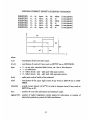
UNIFORM CURRENT DENSITY SOLENOID COMMANDS
SOLENOID,
SOLENOID,
SOLENOID,
SOLENOID,
SOLENOID,
SOLENOID,
rl,
rl,
rc,
rc,
ri,
ri,
z1,
zl,
zc,
zc,
z1,
z1,
isym,
isym,
isym,
isym,
isym,
isym,
dr,
dr,
dr,
dr,
r3,
r3,
dz,
dz,
dz,
dz,
z3,
z3,
cdens
ni
cdens
ni
cdens
ni
(,turn,ngauss)
(,turn,ngauss)
(,turn,ngauss)
(,turn,ngauss)
(,turn,ngauss)
(,turn,ngauss)
z
I
r3
---------------------------I
-----------I
I
rc
I
I
I
-------------I---->+
IdzI
------ri----->1---------I
I
zil
Izc
1z3
I
------------------------------------------
r
where
rl,z1
- coordinates of the lower left corner.
(rc,zc)
- coordinates of centroid if any word on SETUP line is CENTROID.
isym
= 0 - do not plot, calculate fields, forces, etc. due to this element.
= 1 - no reflections.
= 2 - reflect about r axis - split pair with same current.
= -2 - reflect about r axis - split pair with opposing current.
dr,dz
- radial and vertical builds of the solenoid.
r3,z3
- coordinates of the upper right corner if any word on SETUP line is CORNERS.
cdens(ni)
- overall current density (A/m**2) or total ni (ampere-turns) if any word on
SETUP line is NI .
turn
- number of turns (for inductance and resistance only).
ngauss [10) - number of radial integration current sheets for inductance or number of
azimuthal quadrature points for field calculations.
17
UNIFORM CURRENT DENSITY QUAD COMMANDS
QUAD,
QUAD,
r1,z1,r2,z2,r3,z3,r4,z4,
r1,z1,r2,z2,r3,z3,r4,z4,
isym,
isym,
cdens
ni
(,turn,ngauss,nrads)
(,turn,ngauss,nrads)
z
(r4,z4)
-/---------/
I
I
I
I
I
I
/
/
/
/
/
/
/-------/
(rl,zi)
(r3,z3)
/
/
(r2,z2)
where
rl,zl
-
r2,z2
- coordinate pairs of the four corners in counterclockwise order
r3,z3
r4,z4
-
isym
=
=
=
0 - do not calculate fields, etc due to this element
1 - no reflections
2 - reflect about r axis - split pair with same current
= -2 - reflect about r axis - split pair with opposing current
cdens(ni)
- overall current density (A/m**2) or total ni (ampere-turns) if any word on
SETUP line is NI
turn
- number of turns (for inductance and resistance only)
ngauss [10] - number of radial integration current sheets for inductance or number of
azimuthal quadrature points for field calculations
nrads [3]
- number of radial subdivisions of the quadrilateral
The QUAD is treated by breaking the element into nrads (number of radial) rectangular
regions. The user is responsible for picking a reasonable number. The COILS plot with
the OVERLAY option can be used to view both the QUAD and the approximation. See
Example 3.
There is a problem in using GROUP-ENDGROUP commands with an isym=O. The
code counts groups before it checks for isym. Therefore, if there is a data file with a set of
GROUP-ENDGROUP commands, an isym=0 will not suppress the group even if all elements of the group have isym=0. This will cause numbering problems for group-calculated
quantities such as inductance. To cure the problem, delete the GROUP-ENDGROUP commands around coil with an isym=0 or delete the set of coils to be ignored.
18
START
The START command is used to start the (ij) ordering of field output at a pair other
than (1,1). This ordering is used only for plotting. The program expects the input of
istartjstart. The r-z plane is mapped into a logical i-j plane with (ij)=(1,1) at the first
(r,z) point and i increasing with r and j with z. If a single mesh is used to generate a
data set for plotting, this is all transparent to the user. If, however, more than one FIELD
command is used to generate the data, the START command must be used before the
second FIELD command to get the (istartjstart) of the subsequent mesh to be consistent
with the first. See FIELD command and the I (J) option. The form is:
START, istart,
jstart
STOP
The STOP command is used to terminate the program. All files including the PLOT
(if opened) are closed.
TERMINAL
The TERMINAL command allows the user to switch input devices from a file to
terminal. This is particularly useful when many coils need to be defined. An input
is used to invoke setup and to define the coils. After the END command for setup,
file contains the TERMINAL command. The program will echo list the input, set up
coils, and then revert to the interactive mode of input, with the terminal prompts.
the
file
the
the
UNITS
The UNITS command allows the units of length for input and output to be set by the
user. The quantity to be input is the multiplier that converts the input to meters. The
form of the command is:
UNITS, units
For example, if inches are to be used for input and output then the command would be
UNITS, 0.0254.
19
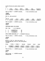
SOLDESIGN EXAMPLES
TERMINAL INPUT AND OUTPUT:
The first example is for a terminal input/output session. A single split pair set of
solenoids is defined. The central field is calculated, and then the force between the two
and system inductance are computed. The input and output shown below are the same as
would appear at the terminal.
$ R USER5:[RDPJ.SOLSOLDESIGN
INPUT FILE NAME (terminal OR t IS ACCEPTABLE)
t
OUTPUT FILE NAME (terminal OR t IS ACCEPTABLE)
t
COMMAND
setup,ni,centroid
SETUP COMMAND (group, symmgroup, endgroup,
solenoid
solenoid, rho, help OR end)
rc,zc,isym,dr,dz,NI
, (turn,ngauss)
1.0, 1.0, 1, 0.1, 0.1, 1.0e6, 1, 5
SETUP COMMAND (group, symmgroup, endgroup,
solenoid
solenoid, rho, help OR end)
rc,zc,isym,dr,dz,NI
, (turn,ngauss)
3.0, 3.0, 1, 0.5, 0.5, 0.5e6, 1, 5
SETUP COMMAND (group, symmgroup, endgroup,
end
Coils =
No.
Time in setup
2 in
=
solenoid, rho, help OR end)
2 groups
7.OOOE-02 seconds,
0 loop calculations used
COMMAND
print
GRP COIL
Rc
Zc
#
#
(im)
( m)
1
1
2
2
1.000
3.000
1.000
3.000
Time in print
=
Delr
(im)
0.100
0.500
Delz
(im)
0.100
0.500
2.OOOE-02 seconds,
NI
(A-t)
1.000E+06
5.OOOE+05
turns
1.OOOE+00
1.OOOE+00
npts
5 1.OOOE+09
5 1.000E+09
0 loop calculations used
COMMAND
field
20
rho
(Ohm-m)
rO,zO,(dr,dz,nr,nz,ipolar,istart,jstart)
2,2
I
1
J
R( m)
1 2.OOOE+00
Time in field
-
Z( m)
Br(T)
2.OOOE+00 -7.3901E-03
Bz(T)
8.9262E-02
4.400E-01 seconds,
B(T)
8.9568E-02
Flux(V-s)
1.8833E+00
0 loop calculations used
COMMAND
peakfield
Coil no.,(nr,nz,iprint)
1
SIDE PT
R( m)
4
3 9.500E-01
Z( m)
Br(T)
1.000E+00 -1.3647E-02
Time in peakfi =
3.580E+00 seconds,
Bz(T)
4.0093E+00
B (T)
4.0093E+00
Flux (V-s)
3.8436E+00
0 loop calculations used
COMMAND
induct
INDUCTANCE MATRIX FOR SYSTEM
COIL
1
1
2
COIL
L or M (Henries)
1
4.0425827D-06
3.7273611D-07
1.0214448D-05
2
2
TOTAL SYSTEM INDUCTANCE IS =
Time in induct =
25
25
25
1.5002503D-05 Henries
1.400E-01 seconds,
0 loop calculations used
COMMAND
force
group no.,(coil no.,intr,intz,iprint) or
loop,ngl,ng2,ninc,(coil no.,intr,intz,iprint)
<return>
Group
1
2
Fr(N/m
)
Fz(N/m
4.7668E+05 1.4420E+04
3.0647E+04 -4.8070E+03
Time in force
)
Rave(m)
1.OOOE+00
3.OOOE+00
-
1.160E+00 seconds,
=
5.420E+00 seconds
1.OOOE+00
3. OOOE+00
dr(m)
1.OOOE-01
5.OOOE-01
dz(m)
1. OOOE-01
5.000E-01
0 loop calculations used
COMMAND
stop
Time in stop
FORTRAN STOP
Zave Cm)
21
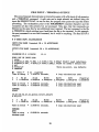
FILE INPUT - TERMINAL OUTPUT
The second example demonstrates an interactive session with a file input of coil geometry
and a TERMINAL command. A split pair and a single solenoid are defined using the
input file EX2INPUT.DAT. As can be seen, the program echo prints the input file before
proceeding. The exclamation point is the SOLDESIGN comment character and the
comments are also echo printed, but not processed. Note also, that the commands are
followed on the same line by any additional input required. The last command in the file
is TERMINAL which switches input back from the file to the terminal. In this example,
the next command is a new field command, but it could be anything. The final STOP is
required.
$ R USER5:[RDPJ.SOL]SOLDESIGN
INPUT FILE NAME (terminal OR t IS ACCEPTABLE)
ex2input
OUTPUT FILE NAME (terminal OR t IS ACCEPTABLE)
t
SOLDESIGN V3.0 11/26/90
10:11
ECHO LIST OF INPUT DATA
1 setup
2 solenoid,0.383,-0.358, 1,0.0166,0.716, 9.954e7 !Didn't need inductance
3 solenoid,0.397, 0.427 8,2,0.0363,0.2382,1.002e8 !so needn't define rest
4 end
5 field,0,0
WOnly one point, use defaults
6 terminal
Coils No.
Time in setup
I
1
3 in
3 groups
= 1.200E-01 seconds,
J3 R( m)
1 0.OOOE+00
Time in field =
Time in termin =
Z( m)
0.OOOE+00
0 loop calculations used
Br(T)
0.0000E+00
4.300E-01 seconds,
0.OOOE+00 seconds,
Bz(T)
2.0001E+00
B (T)
2.0001E+00
Flux (V-s)
0.OOOOE+00
0 loop calculations used
0 loop calculations used
COMMAND
field
rO,zO,(dr,dz,nr,nz,ipolar,istart,jstart)
0.10,0.10
I
1
J
1
R( m)
1.OOOE-01
Z( m)
Br(T)
1.OOOE-01 -1.0390E-05
Time in field
-
2.900E-01 seconds,
COMMAND
stop
Time in stop
FORTRAN STOP
W
8.800E-01 seconds
Bz(T)
2.0001E+00
B (T)
2.0001E+00
Flux (V-s)
6.2835E-02
0 loop calculations used
22
PLOTTING WITH SOLDESIGN
The plotting portion of SOLDESIGN can be used with either batch or interactive
(terminal) input. GRAFLIB is the underlying plot package used by SOLDESIGN. Plotting with SOLDESIGN may be used to generate plots of coil locations, vector plots of
fields or forces, contours of constant flux, total flux density, or flux density components.
In addition, contours of constant field homogeneity may be plotted. These contours in %
are given by (bz-bo)/bo*100, where bo is the value of bz at (ij)=(1,1) which should be
(r,z)=(O,O) for most plots. It may also be used to generate plots of flux, total flux density,
or flux density components versus position (r or z) for fixed z or r. The contour and vector
plots may also include the outlines of the coils.
The contour plotting package can be used to print the coordinates of the contours of
constant (whatever) instead of plotting. This function can serve as a crude contour follower.
The plot package is used to plot the data generated by the FIELD or FORCE commands.
These data may have been just generated or they may have been saved with the SAVE
or SAVEFORCE commands, in which case, the data must be read with the READ or
READFORCE commands, respectively. The (ij) pairs - the first two columns of output
- are essential for the plotting.
In general, coil boundaries will not coincide with the rectangular mesh generated by
a single FIELD command. If nothing were done to get data along the coil boundaries,
the contour and function plots would appear to be incorrect. These routines use linear
interpolation between data points to draw contours or curves. Therefore, if mesh points
do not coincide with coil boundaries, the appropriate components of the flux density will
not appear to experience a jump across the boundaries. SOLDESIGN recognizes this
fact and fills in this data along all coil boundaries. The user need not define meshes
that have lines along coil boundaries. The first time PLOT is called, SOLDESIGN will
generate the required field data so that future plots will be valid in and around coils. If
the SAVE command is used after the PLOT command, all the data including that along
coil boundaries is saved, and future plots using this data will not require the additional
computation.
This filling process is very time consuming and, hence, not very satisfactory. Occasionally it leads to some mysterious effects when the testing fails for some reason or other.
Future versions of SOLDESIGN will incorporate enhancements that make the filling
process more transparent to the user, but for now - what you see is what you get.
NOTE: once the program has filled in data, the original user-defined i-j to r-z mapping
has changed. Care must be taken in the definition of the data to be used in function plots.
The FIELD command mesh for contours has to be purely rectilinear with no missing
data or holes. If other data are to be plotted, minor changes can be made to the package
to make it accept such data.
After the first PLOT command in the interactive mode, SOLDESIGN prompts with:
23
GRAPHICS TERMINAL (y OR n)?
If a supported graphics terminal is being used and plotted output is to be displayed,
then the answer is y. If the answer is y, the program then asks:
SAVE PLOT FILE (y OR n)?
If the plot is to be displayed as well as saved in a file (TEKTRONIX.PLT) the answer is y.
If answer to the first question is n (not a graphics terminal), then plot file is automatically
saved. Similarly, if the graphics input is from a file, the program automatically saves the
file and does not display on the screen.
SOLDESIGN then prompts for a title for all plots. This title must have less than 60
characters. The title will be reproduced at the top of each plot, and is helpful in defining
the run for future reference. The prompt is:
INPUT PLOT TITLE
23456789012345678901234567890123456789012345678901234567890
where the numbers are merely an aid in keeping the title to fewer than 60 characters.
Depending on the default font size, 60 characters may still overflow the line or lines and
be cut off on the plot. A change in font size or in the header is required to eliminate this
truncation - the former requires a program change.
The title can be any combination of letters and numbers. A semicolon (;) within the title
serves as a line feed, and, hence, two-line titles are possible. However, the total number
of characters must be fewer than 60. In general, the second line of a two-line title will
over-write the SOLDESIGN advertisement and not be very aesthetic.
The plotting section uses the same free-field reader as does the main computing section.
That is, numeric and alphabetic variables may be mixed on an input line. Numeric values
or alphabetic words are separated by commas or spaces. The order of entries is important.
Those inputs not specified either by ,, or by < return > are set to the default values (0
unless otherwise specified).
24
The program then prompts for the plot type and other plot information with:
PLOTTYPE, TYPE, rmin, rmax, zmin, zmax (,scale, iout, iprint, DRAW, NOFILL, P,
OVERLAY)
where available PLOTTYPEs are:
COILS, CONTOURS, FUNCTION, VECTORS, HEADER, or END
and where
TYPE
- BR, BZ, B, BX, BY, FLUX, HOMOG (=(bz-bo)/bo*100), or MISC. (see
the READFIELD command for use of MISC option).
rminrmax - the r or x limits of the region to be plotted
zmin,zmax - the z or y limits of the region to be plotted. If PLOTTYPE=FUNCTION,
zmin and zmax are interpreted as the function minimum and maximum,
respectively. If both are entered as zero, the program will calculate the min
and max).
scale
iout[0]
- scale factor for labels [1.0]. If contour labels are desired in gauss scale=1.e+4.
- height of coil (group) numbers on coil plots [65.0].
- length scale for vectors in vector plot [0.12].
- flag for drawing coil outlines on vector and contour plots.
= 0 - omit coils
= 1 - draw coils
if coil plot (TYPE=COILS) then:
= 2 (-2) number groups without (with) coils drawn
= 1 (-1) number coils without (with) coils drawn
= 0 (default) - coil boundaries only
if function plot (TYPE=FUNCTION) then:
= 1 suppress background grid
iprint[0]
flag for printed contour output.
= 0 - normal plotting
-
= 1 - no plotting, but print coordinates of contours.
DRAW
-
see description under CONTOUR plotting. This invocation of DRAW affects
only coil geometry plots. CONTOURS, and VECTORS require the DRAW
option to be specified on the second command line.
NOFILL
-
if NOFILL then the automatic filling of data along the coil boundaries will
not be done. LET THE USER BEWARE!
OVERLAY- a special flag to overlay the nrads radially subdivided rectangular coils used
to model a QUAD element.
25
The major plot types are discussed below in individual sections. The HEADER command is used to change the plot header (title) without exiting the plot package.
The END command is used to terminate the plot section and return control to the
main program. Any subsequent plot command will yield the header prompt, but not the
graphics terminal prompt. New plots are appended to any saved plot. An END, SAVE
command, however, will close the plot file and a subsequent plot command will open a
new plot file if the original request was for a file.
26
COIL PLOTTING
Any coil plots (either outlines in contouring or vector plots or geometry plots) will draw
an X in coils with positive currents - that is, the coil diagonals will be drawn. No diagonals
will be drawn for coils carrying a negative current. A coil with zero current will be drawn
in a dashed line mode. An iout=-1 option will cause the coil diagonals to be suppressed for
positive currents in order to make the vectors (especially force vectors) more apparent. For
coil geometry plotting with coil or group numbers drawn at coil centroids, the diagonals
are automatically omitted.
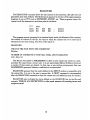
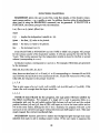
Figure 1 illustrates four sample coil plots. For these samples, the generating command
is shown in the position that usually has the title or header. The coils are defined by the
following sequence of setup commands:
setup,ni,centroid
symmgroup
solenoid, 1.3, 0.4, 2, 0.3, 0.4, 1.e5,
solenoid, 0.5, 0.6, 2, 0.4, 0.2, -1.e5,
quad, 0.20, 0.10, 0.45, 0.20, 0.55, 0.45, 0.16, 0.35, 2, 1.e4, 1, 1, 5
end
The figure in the upper left represents a basic coil plot with no additional options. The
open boxes represent coils with a negative current. The diagonals in a coil imply that the
coil is carrying a positive current.
The figure in the upper right shows the coil numbers at the center of each coil cross
section. The size of the numeric characters can be adjusted using the scale parameter on
the plot command line.
The figure at the lower left shows the coils with the group numbers at the centers. The
negative iout parameter in both this and the previous plot causes the coil outline to be
drawn. A positive iout causes the coil outline to be suppressed.
The final figure shows the OVERLAY option associated with the QUAD option. The
pair of irregularly shaped coils are shown with the five radial "coils" used to model the
QUAD in the field and inductance routines. The use of five subdivisions is arbitrary.
27
COILS. 0.
SOLDESIGN V3.0
2. -1.
1/ 2/91
COILS.I.2. -1. 1. 55 . -1
17.43
1/ 2/91
1
SMLDESIGN V3.0
17:43
I.E
1.9
I..
.8
.8
Eli
.4
.
31
.6
WE
.2
.2
a
0.
...
:
3
0.
-. 2
-. 2
-. 4
LIE
-. 6
-. 6
-. 8
-. 8-
-1.9
-1.
.5
1.9
19 1 mJ
1.5
9.
2.1
.5
1.5
2.0
COILS
COILS
COILS. 0. 2. -1. 1. . OVERLRY
17:43
1/ 2/91
COILS.O.2. -1. 1. 45 . -2
17:43
SOLDESIGN V3.0 1/ 2/91
SOLDESIBN V3.0
.A-
.8
.5
.6-
LI2
W9
.20.I
1.9
.2
U
-
-.
-.4-
W
-. 8 -
I
-1.9
.5
C.
1.9L
19 ( m)
COILS
1.5
.-,
- 1
2.3
2-
0.
-. 6
-
-. 8
-
Wl
-1.9
9.
.5
1.9
C( S
COILS
Fig, 1. SOLDESIGN COIL PLOTTING EXAMPLES
28
1.5
2.0
CONTOUR PLOTTING
If PLOTTYPE=CONTOURS, SOLDESIGN prints the maximum and minimum values of the function within the plot region, and prompts for the necessary data for drawing
and labeling the contours, with the statement:
ncon, (pmin, dp, iplt, htd, lblfrq, ilbl, ndec, intyp, LOG, STYLE, MORE, DRAW) ?
where
ncor
- number of requested contours (0 < Inconl < 100). If ncon < 0, the routine
prompts for input of contours values and linestyles.
pmi
- minimum value (first contour) to be plotted. The default is the program
determined minimum value in the region.
dp
- delta between contours. Calculated default is (pmax-pmin)/ncon
iplt [1000] - measure of number of labels on a contour. Default gives no labels. Iplt
represents a distance between labels expressed as a percentage of the plot
width. E.g. iplt=20 implies the distance between labels is approximately
20% of the plot width.
htd
[55]
- height of label numbers.
lblfrq [2]
- label every lblfrq contour.
ilbl [0]
- =0 label with contour value; =1 label with contour number.
ndec [1]
- number of decimals in label.
Inty p [1]
- line style (see the GRAFLIB manual).
LOG
- contour increment is logarithmic; p(i)=p(i-1)*10.0 for i=2,ncon.
STYLE
- negative, zero and positive values of the function being contoured are drawn
with different line types - light dash, heavy dash, and solid, respectively.
MO RE
- used with MISC to plot more contour data on same axis. Asks for the next
column number to be contoured. Col=0 terminates.
DR AW
- draw outline to be overlayed on contours. Prompts for file(s)
FORMAT 1
FORMAT 2
npts
- Number of points
npts
n,nx,ny,xx,yy
or
xxyy
npts
n,nx,ny,xx,yy
or
npts
xxyy
- Number of points second set
SOLDESIGN accepts multiple sets of data within a file. It also accepts
multiple files. A filename = NONE terminates the outline section.
29
For each file, SOLDESIGN prompts for:
linetype,linesize,xo,yo,xscle,yscle,ifmt
where
linetype[1.]
- GRAFLIB line style
linesize[.4]
- GRAFLIB thickness
xoyo
- origin shifts to account for possible shift in coordinate system between outline and SOLDESIGN
xscle,yscle
- allow stretching of coordinates of the outline. i.e.
xplt = xo + xx xscle and yplt = yo + yy yscle
ifmt
- format flag =1 n,nx,nyxx,yy; =2 xxyy
The scale entry on the plot command can be used to scale contour values. If field
contours in gauss are desired, then scale = 1.e4. If TYPE is MISC, the program will
prompt for a plot title, X-axis title, and Y-axis title, and column number (1 to 4).
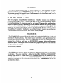
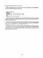
Figure 2 illustrates some of the contouring options of SOLDESIGN. The definition of
the coils and the generating field command are:
setup,ni,centroid
symmgroup
solenoid, 1.3, 0.4, 2, 0.3, 0.4, I.e5,
solenoid, 0.5, 0.6, 2, 0.4, 0.2, -1.e5,
end
field,0.0,0.0,0.05,0.05,41,41
The plot commands are written at the top of each of the four plots in the space where
the plot title is usually placed. As can be seen, the coil boundaries are coincident with the
field mesh. That is, fields are automatically calculated along coil boundaries. Therefore,
the NOFILL option can be safely used in all four of the examples.
The figure in the upper left corner is generated by invoking the simplest of the contour
commands. Fifteen contours of constant flux are requested. SOLDESIGN computes the
minimum and maximum values of flux in the region and calculates the increment. The
first contour (minimum) and increment values are written in the line of text just above the
plot. The iout=1 option on the plot command line is used to superpose the coils on the
contours. The figure in the upper left corner is generated with a similar command, but
fifteen contours of constant B-magnitude are requested.
The figure in the lower left corner is the result of a request for 15 labelled contours of
constant B-magnitude. The starting contour value is required to be zero and the contour
increment is 0.01 T. The frequency of labeling is every 5% of the width of the plot. The
height of the characters is set at 65 (smaller than the default 55). Every other contour is
to be labelled with two decimal places in the label.
NOTE: Specifying contour decimal places must be done with care. Rounding
30
occurs and if a sufficient number of places is not specified, the labels will appear to be
incorrect. For example, a single decimal place for the figure in the lower left corner would
label contours 0.0, 0.0, 0.1, 0.1, 0.1, 0.1, .... corresponding to true values of 0.02, 0.04,
0.06, 0.08, 0.10, 0.12, etc.
The figure in the lower right corner is the same plot, but with the magnitude of B
expressed in gauss. The scaling is accomplished with the 1.e4 scale entry on the CONTOURS command line. NOTE: the change in the dp from 0.01 to 100. Also, the number
of decimal places is set to -1 for an integer form. In addition, the label spacing is set to
10% of the plot width.
31
CONTOURS.fLUX. 0. 2. 0. 2...1.NOFILL
15
coN.ur -1 -
DelT
-5.33K-I2
-
CONTOURS.B.
is
3.520e-02
Contour I
72E~q~
1. 2. 0. 2..
NOFILL
OSIT e
. 581r-f'
-
1.
*
1.U07EI
2.9
.-
1.2
1.6
1.2-
1.2
U
..
1.9
.2
.2
0.
I....
0.
.5
1.5
1.O
0.
2.3
.5
CONTOURS OF FLUlX
1.5
m.O
20
CONTOURS OF B
CONTOURS.B. 0. 2. 0. 2.. 1. NEFILL
15. 0.0. 1.01. 5. 65. 2.. 2
contour 1 -oe
- i.eUIE-oz
2.0
CONTOURS.B. 1. 2. 0. 2. le4.
16. 0. 100. 10. 65. 2..-1
contour i
I..
-
5.emU+i8
1.
Della
NOFILL
1.0Es0IZ
1.2
F
1.8
.02
.02
U
200
1.8
1.2
1.2
1.5
U
1.9
-
-- 0--se
1.6
I...
a
.8
e
2
-. 00---
00
.6
....
0..
.5
1.9
4.,
~
1.5
.5
2.8
CONTOURS OF 8
1.0
CONTOURS OF B
Fig. 2. SOLDESIGN CONTOUR PLOTTING EXAMPLES
32
1.5
2.0
FUNCTION PLOTTING
SOLDESIGN allows the user to plot flux, total flux density, or flux density components versus position - e.g., a profile on axis. In addition, function plots of miscellaneous
data (read in using the READFIELD command) can be generated. If PLOTTYPE is
FUNCTION, the system prompts with the statement:
i or j (for r or z), ijstart, ijfinal, ijnc
where
i (j)
- implies the independent variable is r (z).
j (i) value to be plotted.
the last j (i) value to be plotted.
the increment in j (i).
ijstart - the first
ijfinal
-
ijnc
-
If the PLOTTYPE is FUNCTION and the TYPE is MISC the program will prompt
for the column number of the dependent variable. It will also prompt for the title for the
Y-axis. This routine assumes that the independent variable is stored in the first or second
column (corresponding to r or z).
In this plot routine, i corresponds to r and j to z. For example, if field data are generated
by the statement:
field, 0.0, 0.0, 0.01, 0.01, 21, 21, 0
then, there are data from i=1 to 21 and j=1 to 21 corresponding to r between 0.0 and 0.20
and z between 0.0 and 0.20 in even increments of 0.01. To plot Bz versus z for r=0.0, 0.02,
0.04, 0.06, the response to the prompt would be:
j, 1, 7, 2
That is plot versus z for i=1 (r=0), i=3 (r=0.02), i=5 (r=0.04) and i=7 (r=0.06). If Bz
versus r for z=0 is sought then the input would be:
i, 1, 1, 1
NOTE: If data FILLed by the program, the (ij) pairs will have shifted by
the filled coordinates. For example, if a single coil is used to generate fields on a
rectangular grid, and the coil radial position falls between i=3 and i=4 and the vertical
position between j=2 and j=3, then a FILL will insert an i=4 at the inner radius and an
i=5 at the outer radius, shifting the old i's by 2. Similarly, the program will inset a j=3
and a j=4 at the coil lower and upper vertical extremes and shift larger j's by 2. The user
must request the correct reordered (ij).
SOLDESIGN function plots have a dashed line background grid through each major
(labeled) tick mark to aid in reading numeric values. If the user wants to suppress this
33
grid, then an entry of IOUT=1 can be used.
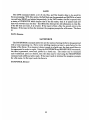
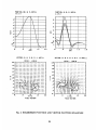
Figure 3 illustrates some of the function and vector plot capabilities of SOLDESIGN.
The coils and field generating command are:
setup,ni,centroid
symmgroup
solenoid, 1.3, 0.4, 2, 0.4, 0.4, 1.e5,
solenoid, 0.5, 0.6, 2, 0.4, 0.2, -1.e5,
end
field,0.0,0.0,0.10,0.10,21,21
The plot commands are written at the top of each of the four plots in the space where
the plot title is placed. The NOFILL option is used in all four of the examples. NOTE: It
must be repeated each time.
The figure in the upper left corner is obtained by requesting a function plot of Bz versus
r or i for j = 1 to 1 with increment 1. That is, the Bz along z = 0 is plotted. SOLDESIGN
will accept the characters "r" or "z" as readily as "i" or
The figure in the upper right corner represents a plot of B-magnitude versus j or z for i =
1, 2 and 3 or for r = 0.0, 0.1, and 0.2, respectively. The present version of SOLDESIGN
does not label curves or change linestyles. However, such a change is relatively easy and
will be made in future versions.
34
FUNCTION, BZ, 0, 2, NOFILL
1.1.1 1
- -------------
- -------- -----
Ij
-
.
-
.~
~..
....................
6.~~
~..
-
3 -------- -- ---------- -------------
I-
FUNCTION, B, 0, 2. NOFILL
J.143.1
-
---
-
-
-
-
--
-- --
-- - -
-
---------
---------------
---------
-
#1 I
3.
....
.
. ....
.....
-- .
-.---- -- - - -
-...
-
2 ------
0
-2
0.
.5
R()
1.5
I.
0
2.1
0..5
VECTORS. B. 5. 2. 0. 2..1. NOFELL
EXIMUN
2.1
.4
'
'
Z (Wi
.AIMLI
-
'
-
-
.
1.5
2.0
VECTORS. B. 0. 2. 0. 2. 0.2. 1.P.NOFILL
1.'4BOE-II
.'
j-.-.----------.-.
2.~
.1
-
-
I.B&-UI
2.
I,
1.8-
1.
I,
r r
E
-o
-0
1. .2t-
.
4
4
'0II*
U
I.
p-a
h.p
.8
+4
+
.6-
.6
~t
.2-
Tr T
94
0..
.
4
.5
.
T
.
.2
or
+4-
I
I-/
- 1
1.0
FI E m)
FIELD VECTORS
1.5
2.1
0.
.5
1.0
1.5
R Vm O
FIELD VECTORS
Fig. 3. SOLDESIGN FUNCTION AND VECTOR PLOTTING EXAMPLES
35
2.0
VECTOR PLOTTING
Vector plots do not require a second command line. For vector plots, the second entry
(TYPE) can be FIELD or FORCE. A third alphabetic input of 'P' may be invoked to
draw the arrowhead proportional to the length of the shank. Otherwise, the arrowhead is
constant in size. The scale option changes the length of the vectors.
The two lower plots in Figure 3 illustrate the use of the VECTORS option. The plot
in the lower left corner is of the magnetic flux density or field vectors with only the coil
outlines as an option. The plot in the lower right corner shows the same information but
with a scale factor of 0.24 instead of the default 0.12 and a arrowhead proportional ("P"
option) to the shank.
36
HINTS AND FURTHER EXPLANATIONS
TURNS, AMPERE-TURNS or CURRENT PER TURN?
The actual number of turns in a coil may not be known explicitly even though the
winding pack envelope and overall current density (or total ampere-turns) are known.
SOLDESIGN was originally written to accept only the overall current density and did
not calculate inductances or resistances. Over the centuries, the NI option and inductance
and resistance calculations were added. For the latter two options, the number of turns
in the coil is needed. Hence, the addition of the turns entry in SETUP. The turns are not
used in the field or force calculations except with the READCURR option.
If SOLDESIGN is used to generate input to other codes such as circuit codes, then
CARE MUST BE TAKEN TO USE THE ENTRIES TURNS AND AMPERETURNS CORRECTLY. Unfortunately, this requires some input file changes depending
on the desired output.
If the total coil inductance and resistance are desired, then the turns entry must be
used. Otherwise, the resulting output is on a per-turn-squared basis - i.e. the loop voltage
equation is on a per-turn basis and the currents in the equation are ampere-turns.
If the field or force influence coefficients (i.e., field components at a point per unit
current in a coil) are desired for use in other postprocessing routines, the ampere-turns
entry is important and the turns are ignored.
Now, here's the problem. If the inductance and resistance matrices have been calculated
using the correct number of turns, then circuit code output is on a current-per-turn basis.
If these currents are to then be used with field or force influence coefficients, then the
SOLDESIGN coefficient run must be made with the NI equal to the number of turns.
That is, the desired output is the field components at a point per unit (turn) current, not
the field per unit ampere-turn. NOTE: if READCURR is used, the currents read from the
file ARE multiplied by the turns on the SOLENOID definition line.
READFIELD and the MISCELLANEOUS OPTION for PLOTTING
The READFIELD and MISC plot options were incorporated into SOLDESIGN to
allow quick access to contour and function plotting routines. SOLDESIGN requires the
format:
i j r(ij) z(ij) data(k),k=1,ncol
where ncol is the total number of data columns in the file. If ncol is greater than 4,
then the program prompts for four columns to be used. This requirement is mandated by
the storage scheme in SOLDESIGN. The scheme is: r(ij), z(ij), br(ij), bz(ij), bt(ij),
flux(ij). The READFIELD routine stores the four columns in the br, bz, bt (mod b),
37
and flux arrays. Therefore, to shortcut some of the MISC plot input such as titles and
column numbers, the regular command such as CONTOURS,FLUX would contour the
-values stored in the fourth array. At this time, there is no MISC option on the VECTOR
command. However, if the desired vector data are read into columns one and two (Br and
Bz), the VECTOR, FIELD option will work.
MULTIPLE FIELD COMMANDS, COIL FILLING, ETC
SOLDESIGN uses two sets of coordinates for calculating, storing, reading and plotting
field quantities. It basically assumes calculations are performed on a rectilinear mesh. The
indices (ij) are used along with the coordinates (r,z). The contouring, vector, and function
plotting routines make use of these two sets of coordinates to make the plotting more efficient. The various plotting functions may be thought of as piecewise linear interpolations
- or connect the dots.
Since SOLDESIGN uses a uniform current density coil, there are no jump changes in
field components across coil boundaries. However, the derivative of the tangential field
component is discontinuous across the boundary. If a field calculation is done with field
points not on the coil boundary, a contour or function plot across the boundary will
"connect the dots" and not show the correct break in slope. The values at both points are
correct, but to get the correct break, the fields need to be calculated on the coil boundary.
An attempt is made in SOLDESIGN to include the coil boundaries correctly, if the
user has not done so. The mesh is expanded to include the boundaries with the appropriate
shifting of the other data. This feature is not particularly efficient and can sometimes cause
mysterious effects. The NOFILL option in the plotting package overrides this option, but
can lead to funny looking plots if a coil does lie within the region of the plot.
One solution is to mesh the original FIELD command(s) so that coil boundaries are
automatically included in the mesh(es). The original inclusion of the START option was
meant to aid the user in using multiple FIELD commands. The recent inclusion of the
istart and jstart options on the FIELD command line is an alternate (and I think better)
way to handle this. A point with the same (ij) and (r,z) can be defined more than once.
Only the last calculation is used in plotting. If this option or the START option are used,
then NOFILL can be used. Indeed, if it is not used, the program tolerances may be such
that SOLDESIGN will attempt to fill anyway.
THE USE OF THE LOOP SWITCH OPTION
The LOOPSW option was added to SOLDESIGN in order to speed up the calculation
of fields, forces, and inductances for a system with a large number of coils. For field
calculations, when the field point is sufficiently far from the coil, a loop calculation is
used rather than the uniform current density formulation. "Sufficiently far" is defined in
SOLDESIGN to mean when the distance from the coil center to the field point, dis, is
38
greater than a user specified tolerance times the coil diagonal, i.e., when dis > tol * dia.
This test is rather arbitrary, but seems to work. The diagonal measure is used to account
for the possibility of a thin, but tall, coil. Typical tolerances of 2 to 5 may be used.
For the calculation of the mutual inductance between coils, the LOOPSW option allows a
smaller number of radial current sheets to be used than that specified on the SOLENOID
definition line. If the distance between coil centers, dis, is greater than tol times the
coil diagonal, the number of sheets specified in the LOOPSW command is used. Testing
on generic problems indicates that two radial sheets with tolerance of 5 give very good
agreement with the mutual from a 5 or 10 sheet integration, with a significant savings in
time.
Errors in field and inductance calculations can be significant if the tolerance or number
of sheets is too small. As always, it is up to the user to make the right choice - this
program is not artificially (or otherwise) intelligent.
GRAFLIB AXIS LABELING ON THE VAX
GRAFLIB was chosen as the underlying graphics package primarily because it was
supported on both the VAXs and the CRAYs. It is a pretty good package. However, the
VAX version has a bug that sometimes rears its ugly head. GRAFLIB chooses the number
of major tick marks on each axis that will be have numeric values printed. Occasionally, a
set is chosen with minimum and maximum values and a label increment that does not get
properly rounded and the result is either a string of 9's or O's or an asterisk plotted as the
tick label. Once in a while, the entire axis line and all tick labels are omitted. The only
cure for this is to replot with a forced scale different from that which lead to the funny
result.
SUBDIVIDING COIL FOR DETAILED FORCE CALCULATIONS
SOLDESIGN has the capability of automatically subdividing coils into a number of
subregions. This addition was meant to allow the user the capability of calculating inductance, resistance, etc., for a rectangular region with multiple elements. It should not be
used to calculate the force distribution over a coil by actually calculating the forces on
a number of subcoils. It is not an efficient process, since the force calculator treats each
subregion as a distinct and independent coil and calculates the field produced by all the
subregions (rather than simply calculating the fields from the overall coil and integrating
only over the subregion).
39
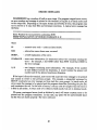
ERROR MESSAGES
SOLDESIGN has a number of built-in error traps. If a program trapped error occurs,
an error number and message is printed to the terminal (or log file in a batch mode) and
to the output file. Depending on the input stream and severity of error, the program may
try to recover or it may close files and terminate execution. A typical error message has
the form:
Error Number iiii encountered in subroutine SUB
BRIEF EXPLANATION OF ERROR COMMAND i1 i2
where
iiii
- numeric error code - codes are listed below.
SUB
- subroutine name where error occurred.
BRIEF...
- a brief explanation of the error.
COMMAND - some more information (10 characters) about the command causing the
error - for example, a line EMD rather than END would have EMD in
the error message.
ii, i2
- two integers containing more information. For example, if the number
of coils defined exceeds the dimension, il would contain the present coil
number and i2 the allowed maximum dimension.
If the input is from the terminal, most errors will cause the error message to be printed
and control to revert to the previous prompt. For example, a misspelled command in
SETUP would print an error message and loop back for a new prompt. In batch mode, all
errors cause the message to be printed and the program closes files (including the plot file)
and terminates the run. In the table of errors, a return code of 0 implies that the error is
is fatal in all modes. A return code of 1 is fatal in batch mode, but not in terminal mode.
Of course, nontrapped errors (such as division by zero) will cause a system error to be
printed and the program terminates. In this case, any plots will be unrecoverable since
the file was not closed properly. The error codes are:
40
U
C)
0
II
w
C)
04
0
8
0
0
u
0
z
z
-e
0
0
I
0
z
0 m
0
D
044
z
0
N
0
H
C,,
0
0
0
~rz1
E-4
E-
0
z
0
o
<
00
pr W
a
0
z
CY
0
z
U
i
z
0
<N
z
0
ii
zr4
H
8
z
I
N
14
I
C,
H
C.) 0
0 0
rxl
N
H
0E H
0
4
z
0
U
-I
0 0
H
rZ4
I0
1-
iii
-I
9a
r-4
r-4
0
0 Q0 Q 0
=
0
r1 -4-4
0
I-I
V-4
0
V-4
-4
--
C.qIem
004T- 'At 10
V-4
4
to
REFERENCES
[1] G. Brown, L. Flax, E. Itean, and J. Laurence, "Axial and Radial Magnetic Fields of
Thick, Finite-Length Solenoids," NASA TR-R-170, Dec. 1963.
[2] M. Garrett,"Calculation of Fields, Forces, and Mutual Inductances of Current Systems
by Elliptic Integrals," Journal of Applied Physics, Vol. 34, No. 9, September, 1963.
[3] W. Smythe, Static and Dynamic Electricity, Third Edition, McGraw-Hill, 1968.
42
HANDY DANDY POCKET GUIDE TO SOLDESIGN COMMANDS
All input is lower case and free-field with comma or space separators. Upper case words
imply alphabetic input; lower case imply numeric.
ENDLIST
FIELD,rO,z,(dr,dz,nr,nz,ipolar,iprint,istart jstart)
FILE,FILENAME
FORCE,group #,(coil #,intr,intziprint)
FORCE,LOOP,grpl,grp2,grpinc,(coil #,intr,intziprint)
HELP
INDUCTigstart,igstopjgstart jgstop
LOOPSW,tol,ngmin
NOLIST
PEAKFIELD,coil #,(nr,nzjprint)
PEAKFIELD,LOOP,ncl,nc2,(nr,nz,iprint)
PRINT
PLOT
GRAPHICS TERMINAL (y OR n)?
if y SAVE FILE (y OR n)?
INPUT PLOT TITLE
PLOTTYPE,TYPE,rmin,rmax,zmin,zmax,(scale,iout,iprint,DRAW,NOFILL)
PLOTTYPE=COILS
TYPE is omitted and no additional input needed
PLOTTYPE=CONTOURS
TYPE=BR, BZ, B, FLUX, HOMOG, or MISC
ncon,(pmin,dp,iplt,htd,lblfrq,ilbl,ndec,lntyp,LOG,STYLE,DRAW,MORE) ?
PLOTTYPE=FUNCTION
TYPE=BR, BZ, B, FLUX, HOMOG, or MISC
I(or J),ijstart,ijfinal,inc
PLOTTYPE=HEADER
TYPE not needed.
PLOTTYPE=VECTORS
TYPE=FIELD or FORCE
PLOTTYPE=END
control returns to SOLDESIGN
READ,FILENAME
READCURR FILENAME
ncirc,time,tol
READFIELD
FILENAME (terminal input)
ncol
if ncol > 4 il,2,i3,i4 (column numbers to be saved)
43
READFORCE,FILENAME
SAVE,FILENAME
SAVEFORCE,FILENAME
SETUP,(NI,CENTROID,CORNERS)
SOLENOIDr1,zl,isym,dr,dz,cdens,(turn,ngauss)
SOLENOID,rl,zl,isym,dr,dz,NI ,(turn,ngauss) if NI
SOLENOID,rc,zc,isym,dr,dz,cdens,(turn,ngauss) if CENTROID
SOLENOID,rc,zc,isym,dr,dz,NI ,(turn,ngauss) if NI & CENTROID
SOLENOID,rl,zl,isym,r3,z3,cdens,(turn,ngauss) if CORNERS
SOLENOID,rl,zl,isym,r3,z3,NI ,(turn,ngauss) if NI & CORNERS
OR
QUAD, ri, zi, r2, z2, r3, z3, r4, z4, isym, cdens, (turn, ngauss, nrads)
QUAD, ri, zi, r2, z2, r3, z3, r4, z4, isym, ni , (turn, ngauss, nrads)
SUBDIVIDE,nnr,nnz
GROUP,rho
ENDGROUP
RHO,rho
SYMMGROUP,rho
END
START,istartijstart
STOP
TERMINAL
UNITS,units
44