Download User Manual∗

User Manual∗
Francesco Russo and Claudia Angelini
CNR-IAC, Naples
March 25, 2014
This work was supported by the Italian Flagship InterOmics Project (PB.P05) and
by BMBS COST Action BM1006.
∗
1
to Luisa
2
Contents
1 Introduction
1.1 Overview of RNASeqGUI R package . . . . . . . . . . . . . .
1.2 Other GUIs for RNASeq data analysis . . . . . . . . . . . . .
1.3 Scope and availability . . . . . . . . . . . . . . . . . . . . . . .
5
5
5
6
2 Installation guide
2.1 For Linux users . . . . . . . . . . . . . . . . . . . . . . . . . .
2.2 For MacOS users . . . . . . . . . . . . . . . . . . . . . . . . .
2.3 For Windows users . . . . . . . . . . . . . . . . . . . . . . . .
6
6
8
8
3 Installation of R and the required R-packages
8
4 Quick start
12
5 Structure of RNASeqGUI main interface
5.1 How to create a new project or select an existing one
5.2 Bam Exploration Section . . . . . . . . . . . . . . . .
5.3 Count Section . . . . . . . . . . . . . . . . . . . . . .
5.4 Pre-Analysis Section . . . . . . . . . . . . . . . . . .
5.4.1 Data Exploration Interface . . . . . . . . . . .
5.4.2 Normalization Interface . . . . . . . . . . . . .
5.5 Data Analysis Section . . . . . . . . . . . . . . . . .
5.5.1 EdgeR . . . . . . . . . . . . . . . . . . . . . .
5.5.2 DESeq . . . . . . . . . . . . . . . . . . . . . .
5.5.3 DESeq2 . . . . . . . . . . . . . . . . . . . . .
5.5.4 NoiSeq . . . . . . . . . . . . . . . . . . . . . .
5.5.5 BaySeq . . . . . . . . . . . . . . . . . . . . . .
5.6 Post Analysis Section . . . . . . . . . . . . . . . . . .
5.6.1 Result Inspection Interface . . . . . . . . . . .
5.6.2 Result Comparison Interface . . . . . . . . . .
5.7 The summary report . . . . . . . . . . . . . . . . . .
13
13
17
21
23
23
26
27
27
29
30
32
33
36
36
38
39
.
.
.
.
.
.
.
.
.
.
.
.
.
.
.
.
.
.
.
.
.
.
.
.
.
.
.
.
.
.
.
.
.
.
.
.
.
.
.
.
.
.
.
.
.
.
.
.
.
.
.
.
.
.
.
.
.
.
.
.
.
.
.
.
.
.
.
.
.
.
.
.
.
.
.
.
.
.
.
.
6 Usage Example
40
6.1 Data Preparation . . . . . . . . . . . . . . . . . . . . . . . . . 40
6.2 Usage of RNASeqGUI . . . . . . . . . . . . . . . . . . . . . . 41
7 How to customize RNASeqGUI
54
7.1 Adding a new button in just three steps . . . . . . . . . . . . 54
8 Technical Details
56
3
Acknowledgement
57
4
1
1.1
Introduction
Overview of RNASeqGUI R package
This manual describes RNASeqGUI R package that is a graphical user interface for the identification of differentially expressed genes from RNA-Seq
experiments.
R (http://cran.r-project.org/) is an open source object oriented language for statistical computing and graphics. RNASeqGUI package includes
several well known RNA-Seq tools, available as command line in www.bioconductor.org.
RNASeqGUI main interface is divided into five sections. Each section is dedicated to a particular step of the data analysis process. The first section covers
the exploration of the bam files. The second concerns the counting process of
the mapped reads against a gene annotation file (GTF). The third focuses
on the exploration of count-data and on data preprocessing, including the
normalization procedures. The fourth is about the identification of the differentially expressed genes that can be performed by several methods, such as:
DESeq, DESeq2, EdgeR, NOISeq, BaySeq. Finally, the fifth section regards
the inspection of the results produced by these methods and the quantitative
comparison among them.
1.2
Other GUIs for RNASeq data analysis
This package was implemented following and expanding the idea presented in
[Villa-Vialaneix et al., 2013] and in http://tuxette.nathalievilla.org/?p=866&lang=en.
The idea of RNASeqGUI is similar to that one presented in [Wettenhall et al., 2004,
Sanges et al., 2007, Lohse et al., 2012, Pramana et al., 2013, Wettenhall et al., 2006,
Angelini et al., 2008] with specific attention on RNA-Seq data analysis. Moreover, RNASeqGUI is designed to facilitate RNA-seq work-flow analysis (via
its organization in several different sections and interfaces and via the inclusions of numerous concise and clear vignettes) and also to facilitate the extensibility of the GUI (via its software development organization that facilitate
the task of expanding and redesign its interfaces). In fact, it is extremely
easy to add new buttons that calls new functionalities. Therefore, a user
can customize RNASeqGUI interfaces for his own purposes and benefits by
adding the methods he needs mostly (for more details see Section 7 How to
5
customize RNASeqGUI: Adding a new button in just three steps).
Hence, we think that RNASeqGUI represents a useful and valid alternative
to other existing GUIs.
1.3
Scope and availability
RNASeqGUI is an R package designed for the identification of differentially
expressed genes across multiple biological conditions. This software is not
just a collection of some known methods and functions, but it is designed
to guide the user during the entire analysis process. Moreover, the GUI is
also helpful for those who are expert R-users since it speeds up the usage of
the included RNA-Seq methods drastically. Current implementation allows
to handle the simple experimental design where the interest is on the experimental condition, future work will cover complex designs.
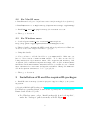
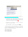
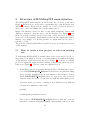
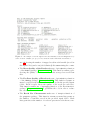
RNASeqGUI is freely available at (see Figure 1) :
http://bioinfo.na.iac.cnr.it/RNASeqGUI/Download
2
Installation guide
RNASeqGUI package requires the RGTK2 graphical library [Lawrence et al., 2010]
to run. The installation process consists in two steps. The first depends on
the operating system (devoted to installation the GTK+ 2.0, an open-source
GUI tool written in C). The second regards the required R packages.
2.1
For Linux users
We tested the RNASeqGUI on Ubuntu 12.10.
1 - Open a terminal and type:
sudo apt-get update
sudo apt-get install libgtk2.0-dev
2 - Type:
sudo apt-get install libcurl4-gnutls-dev
3 - Type:
sudo apt-get install libxml2-dev
4 - Then, go to Section 3.
6
Figure 1: The http://bioinfo.na.iac.cnr.it/RNASeqGUI web page
7
2.2
For MacOS users
1 - Install Xcode developer tools (at least version 5.0.1) from Apple Store (it is free).
2 - Install XQuartz-2.7.5.dmg from http://xquartz.macosforge.org/landing/
3 - Install GTK 2.24.17 X11.pkg from http://r.research.att.com .
4 - Then, go to Section 3.
2.3
For Windows users
1 - download gtk+-bundle 2.22.1-20101229 win64.zip from
http://ftp.gnome.org/pub/gnome/binaries/win64/gtk+/2.22/ .
2 - This is a bundle containing the GTK+ stack and its dependencies for Windows.
To use it, create some empty folder like C : \opt\gtk .
3 - Unzip this bundle.
4 - Now, you have to add the bin folder to your PATH variable. Make sure you
have no other versions of GTK+ in PATH variable. To do this, execute the following instructions: Open Control Panel, click on System and Security, click
on System, click on Advanced System Settings, click on click on Environment
Variables. In the Environment Variables window you will notice two columns
User variables for a user name and System variables. Change the PATH variable in the System variables to be C : \opt\gtk\bin .
5 - Then, go to Section 3.
3
Installation of R and the required R-packages
1 - Install R-3.0.2 from http://cran.r-project.org/ according to your operating system.
2 - Download RNASeqGUI package from http://bioinfo.na.iac.cnr.it/RNASeqGUI/Download.
For Windows operating system, download the zip binary file. For MacOS and
Linux download the tar.gz file.
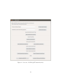
• For Windows users: select “Install packages(s) from local zip files”,
under the “Packages” pull-down menu, as in the Figure 2.
8
Figure 2:
Select “Install packages(s) from local zip files”, under the “Packages” pull-down menu. From
http://outmodedbonsai.sourceforge.net/InstallingLocalRPackages.html
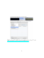
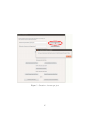
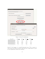
• For MacOS users: under “Package and Data” pull-down menu, select
“Package Installer”. In the “Package Installer”, pull down the top-left
menu, select “Local Binary Package” and navigate to where you have
downloaded the binary package, as in the Figure 3.
• For Linux users: open a shell and go to the directory containing the
package tree and type the command
sudo R CMD INSTALL -l /path/to/library RNASeqGUI 0.0.4
3 - Finally, if the libraries required by RNASeqGUI are not automatically
downloaded and installed, we suggest the user to install all the packages that
are needed to run RNASeqGUI package before loading it. Open R-3.0.2 and
type (the order of the list below is important):
install.packages("e1071")
install.packages("ineq")
install.packages("RGtk2")
install.packages("RCurl")
9
Figure
3:
Under “Package and Data” pull-down menu,
select “Package Installer” and navigate to where you have downloaded the binary package.
From
http://outmodedbonsai.sourceforge.net/InstallingLocalRPackages.html
10
install.packages("digest")
install.packages("ggplot2")
install.packages("RColorBrewer")
install.packages("VennDiagram")
install.packages("XML")
3 - Type (the order of the list below is important):
source("http://bioconductor.org/biocLite.R")
biocLite("biomaRt")
biocLite("DEXSeq")
biocLite("pasilla")
biocLite("GenomicRanges")
biocLite("GenomicFeatures")
biocLite("Rsamtools")
biocLite("edgeR")
biocLite("baySeq")
biocLite("NOISeq")
biocLite("DESeq")
biocLite("DESeq2")
biocLite("gplots")
biocLite("EDASeq")
biocLite("leeBamViews")
biocLite("preprocessCore")
biocLite("scatterplot3d")
biocLite("BiocParallel")
4 - Once the installation is complete, please, check that all the packages listed
above have been installed correctly. To see this, copy and paste the following
list into R-3.0.2 to see whether there are errors coming out.
library(e1071)
library(ineq)
library(RGtk2)
library(e1071)
library(RCurl)
library(digest)
library(ggplot2)
library(RColorBrewer)
library(VennDiagram)
library(XML)
11
library(biomaRt)
library(DEXSeq)
library(pasilla)
library(GenomicRanges)
library(GenomicFeatures)
library(Rsamtools)
library(edgeR)
library(baySeq)
library(NOISeq)
library(DESeq)
library(DESeq2)
library(gplots)
library(EDASeq)
library(leeBamViews)
library(preprocessCore)
library(scatterplot3d)
library(BiocParallel)
In case an error message is displayed, repeat step 3 for the missing packages,
otherwise go to Section 4.
4
Quick start
If you have successfully gone through the installation you are ready to use
RNASeqGUI, as follows.
1 - Open R-3.0.2.
2 - Type
library(RNASeqGUI)
in the R environment. Wait for the package to be loaded.
3 - Finally, type
RNASeqGUI()
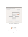
After that, a dialog window, as that one shown in Figure 4, will appear and
you can start interacting with the program.
12
5
Structure of RNASeqGUI main interface
The RNASeqGUI main interface is divided into five Sections, as shown in
Figure 4. Each section corresponds to a particular step of the RNA-Seq data
analysis work-flow. Each section contains one or more Graphical Interfaces
that can be called by clinking the corresponding button.
Inside each interface, there is a How to use this interface button that
displays a vignette to help the user to use the interface (see Figure 10) and
there are several available functionalities (also called functions or methods
in the rest of the manual). Each function takes specific inputs that can be
numeric ones, strings or both and generate an output that can be a plot, a
text file or both.
The sections of RNASeqGUI will be described one by one in the next sections
of this manual.
5.1
How to create a new project or select an existing
one
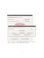
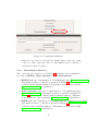
To start using RNASeqGUI, you must either create a new project by choosing a name for it (suppose you choose as name MyProject) and then clicking
on the Create a New Project button (see Figure 5) or select an existing
project by typing the name and then clicking on the Select this Project!
button (see Figure 6). The two cases are explained below.
1. In the first case, if you are using RNASeqGUI for the first time a directory called RNASeqGUI Projects is created in your current working
directory (type getwd() in the R environment to know where you are).
Inside RNASeqGUI Projects directory, a project folder is created
with the name chosen by you (in this case with the name MyProject).
At any moment, you can see or change your working directory with the
following R commands, respectively.
getwd()
setwd("path/you/want/to/set")
The creation of RNASeqGUI Projects directory will only occur the
first time you start using RNASeqGUI. Subsequently, when you click
13
Figure 4: Sections of RNASeqGUI main interface
14
Figure 5: Creation of a new project
15
Figure 6: Selection of an existing project
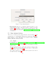
Figure 7: Structure of the MyProject directory
16
the Create a New Project button, RNASeqGUI checks whether the
RNASeqGUI Projects folder already exists in your working directory. If this folder, was already created then RNASeqGUI does not
create a copy of it and all the projects you will create will be stored in
it.
Now, inside RNASeqGUI Projects, you find MyProjects directory. Inside this directory, three folders are automatically created (see
Figure 7), such as: Logs, Results, Plots.
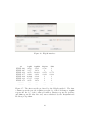
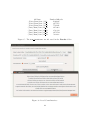
In the Logs folder, a report.txt file is created to report all the actions you perform and which parameters you use by performing those
actions. A session information that summaries all the versions of the
used packages is automatically written in the report.txt file (see Figure 8) at the creation of the project and each time you star this project
again.
2. In the second case, an existing project is selected, see Figure 6. RNASeqGUI checks whether the selected name already exists in the RNASeqGUI Projects folder. If no project with the chosen name is found,
a message warns the user that the selected project does not exist.
When an existing project is restarted, RNASeqGUI continues to write
in the same report.txt file created previously.
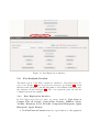
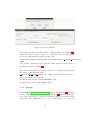
5.2
Bam Exploration Section
In the first section of the GUI, we find the Bam Exploration Interface (see
Figure 9) that can be easily called by clicking the corresponding button. In
this interface we find five different methods to explore the bam files: Read
Counts, Mean Quality of the Reads, Per Base Quality of Reads,
Reads Per Chromosome, Nucleotide Frequencies. Each of these functions takes a folder name as input. This input folder must contain all the
bam files that the user wants to explore. To select the entire bam folder,
select just one bam file inside the bam folder you want to use. The entire
folder will be loaded. To use this interface you can also click on How to use
this Interface button and a vignette window will appear on the screen
describing the interface usage briefly, as shown in Figure 10.
• The Read Counts makes use of barplot function of the graphics
package. This function returns an histogram (as the one shown in Fig17
Figure 8: An example of the file report.txt automatically created in Logs directory
at the creation of MyProject project. Note that the session information is included.
ure 34) showing the number of mapped reads in each bam file (stored in
the input folder) and a txt (tab-delimited) file summarizing the counts.
• The Mean Quality of the Reads makes use of plotQuality function
of the EDASeq package [Risso et al., 2011]. This function returns a plot
showing the quality of each base of the reads averaged across all bam
files.
• The Per Base Quality of Reads makes use of plotQuality function
of the EDASeq package [Risso et al., 2011]. This function returns as
many box-plots as the number of bam files stored in the provided input
folder. Each box-plot shows the quality of the reads per each base.
This function makes use of bplapply function of the BiocParallel
package [Morgan et al., 2014] to parallelize the code in order to reduce
the execution time.
• The Reads Per Chromosome makes use of barplot function of
the graphics package. This function returns as many histograms as
the number of bam files stored in the provided input folder. Each
histogram shows the number of reads are present in each chromosome.
18
Figure 9: By clicking the Bam Exploration Interface button (in the red
cycle), the interface to explore bam files will be displayed.
19
Figure 10: By clicking How to use this Interface button, a vignette window will appear on the screen.
20
This function makes use of bplapply function of the BiocParallel
package [Morgan et al., 2014] to parallelize the code in order to reduce
the execution time.
• The Nucleotide Frequencies makes use of plotNtFrequency function of EDASeq package [Risso et al., 2011]. This function returns a plot
showing the percentage of each nucleotide at each position of the reads.
Figures will be stored in folder Plots, tables in folder Results.
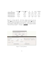
5.3
Count Section
In the second section of the GUI, you find the Count Reads functionality that takes four inputs (see Figure 11). The first input must be the
name of the folder containing the bam files we want to process. The second
input must be an annotation file in GTF format (General Transfer Format). The third input specifies the count mode that can be one of the
following: Union, IntersectionStrict and IntersectionNotEmpty. The
fourth input is Ignore Strand? check-box that allows to perform a strand
specific counting task or not. The Count Reads button calls the function
summarizeOverlaps from the package GenomicRanges [Lawrence et al., 2013]
to obtain gene counts and returns a data-frame, as the one shown in Figure
12. The first column of this data-frame represents the Gene Id, while the
other columns correspond to the names of the loaded bam files. The other entries report the number of reads that have hit a particular gene for each sample (see www.bioconductor.org/packages /release/bioc/vignettes/GenomicRanges/
inst/doc/summarizeOverlaps.pdf for more information about the counting modes).
Read counting can be a very computational demanding task, especially for
large experiments with several samples and big alignment files. The R environment is not optimized from this point of view. Therefore, the counting task can be problematic on standard PC with limited clock speed and
memory space. In this case, it could be beneficial either to process samples independently or to import count tables (in the format specified in
Figure 12) in RNASeqGUI obtained from other tools, such as HTSeq-count
(www-huber.embl.de/users/anders/HTSeq/). Therefore, this function makes
use of bplapply function of the BiocParallel package [Morgan et al., 2014]
to parallelize the code in order to reduce the execution time.
21
Figure 11: Read Count Interface
Gene Id
control 1 control 2 treated 1 treated 2
ENSG00000000003
455
463
583
598
ENSG00000000005
0
0
0
1
ENSG00000000419
1174
1210
1545
1533
ENSG00000000457
260
256
305
349
ENSG00000000460
550
607
709
741
.......................
.....
.....
.....
.....
.......................
.....
.....
.....
.....
Figure 12: An example of a count file with 20062 genes. The row names are
given by the Gene Id in the annotation file (gtf), the column names are given
by the alignment file names (the bam files)
22
Figure 13: Data Exploration Interface
5.4
Pre-Analysis Section
The third section of the GUI contains two interfaces: Data Exploration Interface (see Figure 13) and Normalization Interface (see Figure 14). Both
interfaces take an input count file that must be tab-delimited and must have
the structure shown in Figure 12. The rows represent genes ids and the
columns represent the samples.
5.4.1
Data Exploration Interface
In Data Exploration Interface there are twelve methods: Plot Pairs of
Counts, Plot all Counts, Count Distr, Density, MDPlot, MeanVarPlot, Heatmap, PCA, PCA3D, Component Histogram, Qplot
Histogram, Qplot Density.
• The Plot Pairs of Counts makes use of plot function of the graphics
23
package. This function takes a count file as input (in txt or cvs format)
where the rows correspond to the gene ids and the columns correspond
to the samples. This function also takes two integers, one specifying
Column1 and the other specifying Column2 of the count file (see Figure
13) and plots the counts of sample in Column1 against the counts of
sample in Column2. Moreover, for this function it is possible to plot
either the raw counts or the log of the counts (we add 1 to each number
in the count file to avoid the problem of log(0) ).
• The Plot all Counts makes use of plot function of the graphics
package. This function takes a count file as input and produces all
possible plots that can be generated by each column in the file against
all the other columns. If the input text file has n columns then n(n−1)
plots will be produced. An example of this plot is shown in Figure 41.
For this function, the log check box does not change anything.
• The Count Distr makes use of boxplot function of the graphics
package. This function takes a count file as input and generates a
box plot showing the distribution of the counts for each column in the
file. An example of this plot is shown in Figure 39. Moreover, for this
function it is possible to generate the box plot either of the raw counts
or the log of the counts (we add 1 to each number in the count file to
avoid the problem of log(0) ).
• The Density makes use of density function of the stats package.
This function takes a count file, and a sample specified by an integer
in Column1 as input and produces a curve representing the density
function of the counts for the selected sample. The method is available
in two modes. By default the log of the counts (we add 1 to each
number in the count file to avoid the problem of log(0) ) will be used
to generate the density function. It is possible to uncheck this mode
by clicking in the log? check-box (see Figure 13).
• The MDPlot makes use of MDplot function of the EDASeq package
[Risso et al., 2011]. This function takes a count file and two integers
Column1 and Column2 and returns a plot showing the mean of the
two selected columns against their difference gene by gene. For this
function, the log check box does not change anything.
• The MeanVarPlot makes use of meanVarPlot function of the EDASeq
package [Risso et al., 2011]. This function takes a count file and returns
a plot showing the mean of all columns found in the file against the
24
variance gene by gene. For this function, the log check box does not
change anything.
• The Heatmap makes use of heatmap function of the stats package.
This function takes a count file and an integer N in the How many genes
in the Heatmap? field. The function returns an heat-map of the Nth
most expressed genes (on average). The columns of the heatmap are
the samples, while the rows in the heat-map represent the gene ids of
the most expressed ones. An example of heat-map is shown in Figure
43. Moreover, for this function it is possible to generate the heatmap
either of the raw counts or the log of the counts (we add 1 to each
number in the count file to avoid the problem of log(0) ).
• The PCA makes use of prcomp function of the stats package. This
function takes a count file, a comma separated sequence of strings (e.g.:
a,b,c,d) indicating what are the labels for the legend, to be specified in
the field Factors (see Figure 13) and Legend position in PCA that
can be: topright, bottomright, topleft, bottomleft. The PCA function
returns the principal component analysis plot between the first two
components. An example of PCA plot is shown in Figure 42. For this
function, the log check box does not change anything.
• The PCA3D makes use of scatterplot3d function of the scatterplot3d
package. This function takes the same inputs of the PCA function and
returns the 3D PCA plot between the first, the second and the third
principal component. For this function, the log check box does not
change anything.
• The Component Histogram makes use of screeplot function of
the stats package. This function takes a count file and returns an histogram showing the variance level of each component. For this function,
the log check box does not change anything.
• The Qplot Histogram makes use of qplot function of the ggplot2
package. This function takes a count file and and returns an histogram
showing the count level of each column in the count file. Moreover, for
this function it is possible to generate the histogram either of the raw
counts or the log of the counts (we add 1 to each number in the count
file to avoid the problem of log(0) ).
• The Qplot Density makes use of qplot function of the ggplot2 package. This function takes a count file and and returns a plot showing
the density function of each column in the count file. Moreover, for this
25
Figure 14: Normalization Interface
function it is possible to generate the density either of the raw counts
or the log of the counts (we add 1 to each number in the count file to
avoid the problem of log(0) ).
5.4.2
Normalization Interface
The Normalization Interface (see Figure 14) includes four normalization
procedures: RPKM, Upper Quartile, TMM, Full Quantile.
• RPKM makes use of rpkm function of the NOISeq package [Tarazona et al., 2011].
This function takes a count file as specified in Figure 12 and returns a
count file with normalized numbers. This function performs the RPKM
[Mortazavi et al., 2008] normalization.
• Upper Quartile makes use of uqua function of the NOISeq package
[Tarazona et al., 2011]. This function takes a count file as specified in
Figure 12 and returns a count file with normalized numbers. This function performs the Upper Quartile [Bullard et al., 2010] normalization.
• TMM makes use of tmm function of the NOISeq package [Tarazona et al., 2011].
This function takes a count file as specified in Figure 12 and returns a
count file with normalized numbers. This function performs the TMM
[Robinson et al., 2010] normalization.
26
Figure 15: Data Analysis Interface
• Full Quantile makes use of normalize.quantiles function of the
preprocessCore package. This function takes a count file as specified
in Figure 12 and returns a count file with normalized numbers. This
function performs the Full Quantile [Bolstad et al., 2003, Smyth et al., 2005]
normalization.
5.5
Data Analysis Section
This section contains the Data Analysis Interface shown in Figure 15 and
represents the core of RNASeqGUI. This interface includes five different statistical methods to detect differentially gene expression such as: EdgeR,
DESeq, DESeq2, NoiSeq, BaySeq.
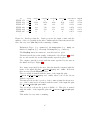
5.5.1
EdgeR
• The EdgeR method [Robinson et al., 2007, Robinson et al., 2008, Robinson et al., 2010,
McCarthy et al., 2012] (see Figure 16) takes an input count file (as the
one shown in Figure 12) via the Open button and returns two text files
and two plots.
The first text file shows the overall result obtained by edgeR (see Figure 17), while the second text file extracts the subset of differentially
expressed genes only (see Figure 18).
The output count file is saved with the name specified by the user in
the Name? field (see Figure 16).
27
Figure 16: EdgeR interface
id
ENSG..003
ENSG..005
ENSG..419
ENSG..457
ENSG..460
ENSG..938
ENSG..971
.............
.............
logFC logCPM
0.023
9.181
2.357
1.058
0.072
10.003
-0.043
8.418
-0.0006 9.164
2.5e-15 0.888
0.078
1.472
.....
.....
.....
.....
PValue
0.736
1
0.178
0.612
1
1
1
.....
.....
FDR
1
1
0.571
0.966
1
1
1
.....
.....
Figure 17: The first text file produced by the EdgeR method. The first
column reports the gene ids, logFC reports the log of the fold-changes, logCPM
reports the the log of the counts per million, PValue reports the p-values
and FDR reports the false discovery rates calculated by the Benjamini and
Hochberg’s algorithm.
28
id
logFC logCPM
ENSG..3756 -0.151 10.652
ENSG..4777 -0.523
8.455
ENSG..5961 -0.506
6.340
ENSG..6025 -0.577
8.699
ENSG..6047 -0.627
6.027
ENSG..6118 -0.152 10.456
ENSG..6282 -0.418
9.966
.............
.....
.....
.............
.....
.....
PValue
0.001
2.6e-10
0.002
2.8e-14
0.001
0.001
1.0e-14
.....
.....
FDR
0.035
4.3e-08
0.049
7.1e-12
0.027
0.039
3.3e-12
.....
.....
Figure 18: The EdgeR second text file showing the differentially expressed
genes only. Columns are the same as in Figure 17.
If no name is specified by the user, then the first output count file is
named with the name of the input file plus “ results EdgeR.txt” suffix. The second file is named with the name of the input file plus
“ fdr=0.05 DE genes EdgeR.txt” suffix, where 0.05 is the chosen FDR.
Both text files are saved in the Results folder.
The first plot shows the Biological Coefficient of Variation for a given
CPM (Count Per Million) and is named with the name of the input
file plus “ Dispersion EdgeR.pdf” suffix. The second plot shows the
relative similarities of the samples and is named with the name of the
input file plus “ MDS EdgeR.pdf” suffix. Both plots are saved in the
Plots folder.
5.5.2
DESeq
• The DESeq method [Anders et al., 2010] (see Figure 19) takes an input count file (as the one shown in Figure 12) via the Open button and
returns two text files and a plot.
The first text file shows the results of this method (see Figure 20), while
the second text file shows the differentially expressed genes only.
The output count file is saved with the name specified by the user in
the Name? field (see Figure 19).
If no name is specified by the user, then the first output count file
is named with the name of the input file plus “ results DESeq.txt”
suffix.
29
Figure 19: DESeq interface
The second file is named with the name of the input file plus
“ padj=0.05 DE genes DESeq.txt” suffix, where 0.05 is the chosen pvalue adjusted.
Both text files are saved in the Results folder. The generated plot
shows the dispersion value for a given mean of normalized counts.
This plot is named with the name of the input file plus “ Dispersion DESeq.pdf”
suffix and it is saved in the Plots folder.
5.5.3
DESeq2
• The DESeq2 method [Anders et al., 2010] (see Figure 21) takes an
input count file (as the one shown in Figure 12) via the Open button
and returns two text files and three plots.
The first text file shows the results of this method (see Figure 20), while
the second text file shows the differentially expressed genes only.
The output count file is saved with the name specified by the user in
the Name? field (see Figure 21).
If no name is specified by the user, then the first file is named with the
30
baseMean
baseMeanA
baseMeanB
foldChange
log2FoldChange
ENSG...0003 625.025
ENSG...0005
0.264
ENSG...0419 1106.882
ENSG...0457 367.367
ENSG...0460 617.493
....
.....
....
.....
id
630.902
0.528
1136.118
362.361
618.055
.....
.....
619.147
0
1077.646
372.374
616.931
.....
.....
0.981
0
0.948
1.027
0.998
.....
.....
-0.027
-Inf
-0.076
0.039
-0.002
.....
.....
Figure 20: DESeq output. The first column reports the gene ids, baseMean
reports the mean normalised counts, averaged over all samples from both
conditions, baseMeanA reports the mean normalised counts from condition
A, baseMeanB mean normalised counts from condition B, foldChange reports the fold changes from condition A to B, log2FoldChange reports the
logarithm (to basis 2) of the fold changes, pval reports the p values for the
statistical significance and padj reports the p values adjusted for multiple
testing calculated by the Benjamini-Hochberg algorithm.
Figure 21: DESeq2 interface
31
pval
padj
0.774
1
0.985
1
0.297 0.935
0.744
1
0.982
1
.....
...
.....
...
id
baseMean
ENSG00000000003 625.025
ENSG00000000005
0.264
ENSG00000000419 1106.882
ENSG00000000457 367.367
ENSG00000000460 617.493
.......................
.....
.......................
.....
log2FoldChange
-0.025
-0.014
-0.072
0.035
-0.002
.....
.....
lfcSE
0.079
0.020
0.062
0.095
0.079
.....
.....
stat pvalue
-0.318 0.750
-0.675 0.499
-1.174 0.240
0.365
0.714
-0.033 0.973
.....
.....
.....
.....
Figure 22: DESeq2 output. The first column reports the gene ids, baseMean
reports the base mean over all rows, log2FoldChange reports the logarithm
(to basis 2) of the fold changes, lfcSE reports the standard errors, stat
reports the Wald statistic, pval reports the p values for the statistical significance and padj reports the p values adjusted for multiple testing calculated
by the Benjamini-Hochberg algorithm.
name of the input file plus “ results DESeq2.txt” suffix. Both text
files are saved in the Results folder.
The second file is named with the name of the input file plus
“ padj=0.05 DE genes DESeq2.txt” suffix, where 0.05 is the chosen
adjusted p-value for rejection.
The first plot shows the dispersion value for a given mean of normalized
counts and it is named with the name of the input file plus
the “ Dispersion DESeq2.pdf” suffix.
The second plot shows the dispersion mean value for a given mean of
normalized counts and it is named with the name of the input file plus
the “ Dispersion Mean DESeq2.pdf” suffix.
The third plot shows the dispersion local value for a given mean of
normalized counts and it is named with the name of the input file plus
the Dispersion Local DESeq2.pdf suffix.
All plots are saved in the Plots folder.
5.5.4
NoiSeq
• The NoiSeq [Tarazona et al., 2011] method (see Figure 23) takes an
input count file (as the one shown in Figure 12) via the Open button
and returns two text files.
32
padj
0.954
0.911
0.768
0.937
0.994
....
....
Figure 23: NoiSeq Interface
The first text file shows the results of this method (see Figure 24),
where M is the log2 ratio of the two conditions. The second text file
shows the differentially expressed genes only.
The first file is named with the name of the input file plus “ results Noiseq.txt”
suffix.
The output count file is saved with the name specified by the user in
the Name? field (see Figure 23).
If no name is specified by the user, then the second file is named with
the name of the input file plus
“ prob=0.8 DE genes Noiseq.txt” suffix, where 0.8 is the chosen posterior probability for rejection.
Both text files are saved in the Results folder.
Both plots are saved in the Plots folder.
5.5.5
BaySeq
• The BaySeq [Hardcastle et al., 2010] method (see Figure 25) takes an
input count file (as the one shown in Figure 12) via the Open button, a list of factors (e.g. treated,treated, control,control) in the
Factors? field, a NDE list (e.g. 1,1,1,1), a DE list (e.g. 1,1,2,2), an
33
id
control mean
ENSG00000000003
575.05
ENSG00000000005
0.22
ENSG00000000419
1000.84
ENSG00000000457
345.75
ENSG00000000460
572.81
.......................
.....
.......................
.....
treated mean
582.71
0.47
1049.17
334.47
570.80
.....
.....
M
D
prob ranking
-0.019 7.659 0.104
-7.659
-1.083 0.251 0.037
-1.112
-0.068 48.333 0.405 -48.333
0.047 11.275 0.164 11.275
0.005 2.004 0.028
2.004
.....
.....
....
....
.....
.....
....
....
Figure 24: NoiSeq result file. The first column reports the gene ids,
control mean is the mean across the control samples, treated mean is the
mean across the treated samples, M is the log2-ratio of the means of the two
conditions) and D is the difference between the two conditions means, prob is
the probability of differential expression, the
√ ranking is a summary statistic
of M and D values (equal to −sign(M) × M 2 + D 2 ).
Figure 25: BaySeq Interface
34
id
ENSG..971
ENSG..419
ENSG..457
ENSG..003
ENSG..460
ENSG..005
......
......
rowID
row
row
row
row
row
row
...
...
7
3
4
1
5
2
control 1
control 2
treated 1
treated 2
Likelihood
FDR.DE
1
1132
354
633
618
0
...
...
1
1070
348
590
580
1
...
...
1
1088
392
618
653
0
...
...
1
1138
377
661
621
0
...
...
0.261
0.217
0.111
0.074
0.067
0.051
....
...
0.738
0.760
0.803
0.833
0.853
0.869
....
....
Figure 26: BaySeq result file. Bayseq reports the input counts and the
number of the row (rowID) in the first columns and the Likelihood and the
false discovery rate (FDR.DE) in the remaining columns.
Estimation Type? (e.g. quantile), the SampleSize (e.g. 1000), an
FDR level, SampleA (e.g. treated) and SampleB (e.g. control).
The BaySeq function returns two text files and two plots.
The first text file shows the results of this method (see Figure 26), while
the second text file shows the differentially expressed genes only.
The output count file is saved with the name specified by the user in
the Name? field (see Figure 25).
If no name is specified by the user, then the first file is named with the
name of the input file plus “ results BaySeq.txt” suffix. Both text
files are saved in the Results folder.
The second file is named with the name of the input file plus
“ fdr=0.05 DE genes BaySeq.txt” suffix, where 0.05 is the chosen
FDR for rejection..
The first plot shows the log ratios of the counts against the mean average of the counts and it is named with the name of the input file plus
the PlotMA BaySeqNB.pdf suffix.
The second plot shows the posterior likelihood. This plot is named
with the name of the input file plus the Posteriors BaySeqNB.pdf
suffix.
This method is very time consuming.
35
Figure 27: Result Inspection Interface
5.6
Post Analysis Section
In the fifth section of the GUI, called Post Analysis Interface, there are
two interfaces: Result Inspection Interface (see Figure 27) and Result
Comparison Interface (see Figure 29). The first interface includes the
possibility to generate several plots for each methods. The second allows to
compare the outcomes obtained from several methods.
5.6.1
Result Inspection Interface
To explore the results of a specific method, we have to click on the used
method in Data Analysis Section (say EdgeR) and the interface in Figure
27 will display the functions available for the selected method (for EdgeR
Plot FC, FDR Hist, P-value Hist functions are available). If we click all
buttons in Figure 27, the interface will grow and we get the interface shown
in Figure 28.
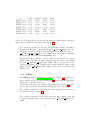
Therefore, for each method, we have Plot FC, FDR Hist (or P-value
Hist) and Volcano Plot functions, except for the BaySeq method since
this method already provides an MAplot and a PosteriorPlot during the
analysis process that can be run in the BaySeq Analysis Interface.
36
Figure 28: Result Inspection Interface after clicking all the five buttons at
the top.
37
Figure 29: Result Comparison Interface
For each function (e.g.: FDR Hist, P-value Hist, Likelihood Hist) of
each method, we just need to provide a “full result” file placed in the Results
folder. For Volcano Plot and Plot FC functions, we must provide a path
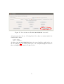
to a “full result” file (as the one shown in Figure 17) and a FDR, P-value or
Prob value (it depends on the chosen method) to point out the differentially
expressed genes (shown in red). In this case, it is also possible to provide a
gene id, provided into the Gene Id field, to point out that particular gene in
the Volcano or FC plot (that gene will be displayed in green).
All generated plots are saved in pdf format in the Plots folder.
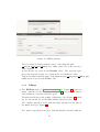
5.6.2
Result Comparison Interface
The second interface includes the possibility to generate Venn diagrams of
either two or three result text files (See Figure 29).
The user must provide two or three text files reporting the results of the
used methods and the corresponding labels to recognize these files in the
generated diagrams.
A Venn diagram is generated and saved in the Plots folder. Moreover, a
text file (showing the gene ids belonging to the intersection of the selected
methods) is created and saved in the Results folder.
38
5.7
The summary report
All the functionalities used by the user are automatically saved in a report
file (as the one shown in Figure 8) inside the Logs directory of the user
project. This report reports the session information that describes all used
package versions by RNASeqGUI at the time of the project creation, along
side with the name of the project, time, date and the parameters (fdr, padj,
etc.) the user selected during the usage of the GUI.
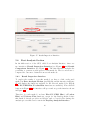
39
Figure 30: At http://bioinfo.na.iac.cnr.it/RNASeqGUI/Example we
can download the example.
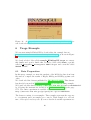
6
Usage Example
We can start using RNASeqGUI by downloading the example data at
http://bioinfo.na.iac.cnr.it/RNASeqGUI/Example, as shown in Figure
30.
We download the folder called example RNASeqGUI.tar.gz, we extract
this bundle and open it. Inside this, we find a folder called demo, a gtf file
called 2L Drosophila melanogaster.BDGP5.70.gtf and a text file called
README.txt file.
6.1
Data Preparation
In this usage example, we start the analysis of the RNA-Seq data from bam
files and we compare the results of EdgeR, DESeq and NOISeq against each
other.
We downloaded the dataset published by [Brooks et al., 2011]. This dataset
has already been used in [Anders et al., 2013] as a real data working example.
We downloaded the data from http://www.ncbi.nlm.nih.gov/sra?term=SRP001537
by following the instructions described in [Anders et al., 2013] at the page
1771. The entire experiment is available at
http://www.ncbi.nlm.nih.gov/geo/query/acc.cgi?acc=GSE18508.
The dataset consists of seven samples. Three samples represent the response
to a treatment and four samples are controls. Each sample is a cell culture of Drosophila melanogaster (For more details about this experiment see
40
BamFileName NameOfTheReducedBam
CG8144 RNA-1
2L 1
CG8144 RNA-3
2L 3
CG8144 RNA-4
2L 4
Untreated-1
2L U1
Untreated-3
2L U3
Untreated-4
2L U4
Untreated-6
2L U6
LibraryType
treated
treated
treated
untreated
untreated
untreated
untreated
LibraryLayout
single
paired
paired
single
paired
paired
single
Figure 31: Experimental design
[Brooks et al., 2011]).
We downloaded and aligned the fastq files by running tophat2 [Kim et al., 2013]
as described in [Anders et al., 2013] at page 1774. Once the bam files were
obtained (we called them CG8144 RNA-1, CG8144 RNA-3, CG8144 RNA-4,
Untreated-1, Untreated-3, Untreated-4, Untreated-6 as in in [Anders et al., 2013]),
it is possible to perform the analysis with RNASeqGUI.
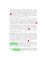
For illustrative purpose and for keeping the computational cost of the
demonstrative example under control, we limit our attention to chromosome
2L. Alignment data (bam files) are contained in the folder called demo inside
the Bam folder, with the following names: 2L 1.bam, 2L 3.bam, 2L 4.bam,
2L U1.bam, 2L U3.bam, 2L U4.bam, 2L U6.bam (see Figure 31).
6.2
Usage of RNASeqGUI
We open R-3.0.2, then we type
library(RNASeqGUI)
and we type
RNASeqGUI()
Once the main RNASeqGUI interface (see Figure 4) has appeared on the
screen, we create a new project (for instance, we can call it demoProject)
and then we click on Bam Exploration Interface button. We select the
demo folder with the Open button. After that, we start the analysis by using the Read Counts button in the Bam Exploration Interface. This action
creates the plot shown in Figure 34. The bam files in the demo folder are
41
Figure 32: Mean Quality of Reads of the bam files stored in the folder
demo without the 2L 1.bam file.
loaded in alphabetically order and their name are displayed at x axis in Figure 34 alphabetically. This plot is automatically saved in pdf format in the
Plots folder of the project you selected.
A text file is also generated and saved in the Results folder with the demo Read
Count.txt name, as shown in Figure 35. This file shows the number of reads
for each bam file.
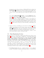
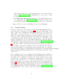
Critical: We cannot use the Mean Quality of Reads or Per Base Quality of Reads function for this dataset, since the
2L 1.bam file was generated by pulling fastq files containing reads of different length (This file correspond to CG8144 RNAi-1
at page 1774 of [Anders et al., 2013]). To use these functions, we need bam files containing reads of the same length.
Otherwise, we get the following error:
Error in as.vector(x, "character"):
cannot coerce type ’environment’ to vector of type ’character’.
If the user wants to use these functions, in this case the 2L 1.bam file must be temporary removed from the demo folder
before using them. In this case, if we use those functions without the 2L 1.bam file, we get the plots in Figure 32 and in
Figure 33, respectively.
Subsequently, we click on Read Count Interface and select the bam folder
demo and the 2L Drosophila melanogaster.BDGP5.70.gtf annotation file.
We select Union as Counting Mode and check the Ignore Strand box, as
shown in Figure 36. Hence, we click on Count Reads button. As result of
42
Figure 33: Per Base Quality of Reads of the bam files stored in the folder
demo without the 2L 1.bam file.
Read Count Histogram
1.2e+07
1.0e+07
8.0e+06
6.0e+06
4.0e+06
2.0e+06
../Data/Bam/e1/2L_U6
../Data/Bam/e1/2L_U4
../Data/Bam/e1/2L_U3
../Data/Bam/e1/2L_U1
../Data/Bam/e1/2L_4
../Data/Bam/e1/2L_3
../Data/Bam/e1/2L_1
0.0e+00
Figure 34: Read Count Histogram of the bam files stored in the folder demo.
43
fileName
NumberOfReads
../Data/Bam/demo/2L 1
12320205
../Data/Bam/demo/2L 3
6477978
../Data/Bam/demo/2L 4
7741241
../Data/Bam/demo/2L U1
9473462
../Data/Bam/demo/2L U3
6586330
../Data/Bam/demo/2L U4
6071744
5883666
../Data/Bam/demo/2L U6
Figure 35: The demo ReadCount.txt file saved in the Results folder.
Figure 36: Read Count Interface.
44
id
FBgn0000018
FBgn0000052
FBgn0000053
FBgn0000055
FBgn0000056
FBgn0000061
FBgn0000075
FBgn0000097
....
....
2L 1
528
2300
2361
1
0
4
2
3849
....
....
2L 3 2L 4 2L U1 2L U3
485 546
613
441
2968 3555 2921
3097
2982 3790 2307
2352
0
0
0
0
0
0
0
0
2
2
1
1
2
1
4
4
3727 4546 4656
4227
....
....
....
....
....
....
....
....
2L U4
501
3244
2542
0
0
5
3
3448
....
....
2L U6
485
2626
1856
0
0
0
1
2569
....
....
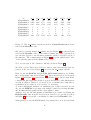
Figure 37: The 2L counts.csv file created by Count Reads function and
saved in the Results folder.
this action, a text file named 2L counts.csv (see Figure 37) is generated and
saved in the Results folder. A file named counts.txt is also generated in
case the user forgets to use the Save Results? check-box at the bottom of
the interface. The column names in Figure 36 follow the alphabetical order
of the bam files placed in the demo folder.
Now, we can explore the obtained count file, shown in Figure 37.
We click on Data Exploration Interface button. Once this interface has appeared on the screen (see Figure 38), we select the 2L counts.csv file.
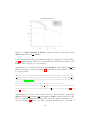
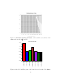
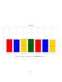
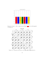
First, we use the BoxPlot and the Plot All Counts functions by clicking
the corresponding buttons (see Figure 38). The generated plots are shown in
Figure 39 and Figure 41, respectively. From Figure 39, we can see that all the
count means (the black lines in the box plot) and all the count distributions
are almost aligned. Therefore, we decide not to normalize the counts since a
normalization procedure does not seem to be necessary.
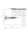
To better understand whether a normalization procedure is needed, we can
also use the MDPlot by plotting each sample counts (by selecting Column1
and Column2 fields) against all the other sample counts.
Anyway, if we use the full quantile normalization procedure by clicking the
Full Quantile button in the Normalization Interface, we get the plot show
in Figure 40 and a text file of normalized counts saved in Results folder.
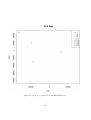
Subsequently, we use the PCA function by typing the 1,3,4,U1,U3,U4,U6
45
Figure 38: Data Exploration Interface
sequence in the PCA Factors? field (see Figure 38) to specify the labels that
will be displayed in the legend at the top-right of the plot generated by this
function (shown in Figure 42).
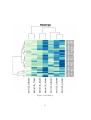
Finally, we can use the HeatMap function to see what are the first (say
thirty) most expressed genes. Therefore, we typed the number 30 in the How
many genes in the Heatmap? field (see Figure 43). From the heatmap, we
can notice that the the most expressed gene is the one called FBgn0000559
(look at the bottom of the Figure 43).
Now, we can start with the analysis. We decide to use EdgeR, DESeq and
NOISeq and compare the results among them.
We click on Data Analysis Interface button.
We start the EdgeR analysis by clicking on the EdgeR button. In the EdgeR
Analysis Interface, we select the 2L counts.csv count file.
We type the T,T,T,U,U,U,U sequence in the Factors? field to specify which
are the treated samples (called T) and which are the untreated ones (called
U) as reported in Figure 31. We choose a 0.05 value as the FDR. Finally, we
click on Run EdgeR button. The EdgeR analysis is performed and two
result text files are created and saved in the Results folder.
46
Figure 39: Box plot generated by the BoxPlot function.
47
Figure 40: Boxplot of the counts shown in Figure 39 after the full quantile
normalization.
Figure 41: Count plots generated by the Plot All Counts function.
48
Figure 42: PCA plot generated by the PCA function.
49
Figure 43: Heatmap
50
We click on DESeq button. In the DESeq Analysis Interface, we select
the 2L counts.csv count file. We type the T,T,T,U,U,U,U sequence in the
Factors? field to specify the treated and untreated samples as in EdgeR
analysis. We type single-end,paired-end,paired-end,single-end,pair
ed-end,paired-end,single-end in the LibTypes field to specify the library
layout as reported in Figure 31. We choose a 0.05 value as the Padj. Finally,
we click on Run DESeq button. The DESeq analysis is performed and two
result text files are created and saved in the Results folder.
We click on NOISeq button. In the NOISeq Analysis Interface, we select
the 2L counts.csv count file. We type the T,T,T,U,U,U,U sequence in the
Factors? field. We type T1,T3,T4,U1,U3,U4,U6 in the TissueRun field to
specify the library layout as specified in Figure 31. We select biological in
the Replicate? field. We choose a 0.6 value as the prob. Finally, we click
on Run NOISeq button. The NOISeq analysis is performed and two result
text files are created and saved in the Results folder.
Once all the results have been obtained, we can start inspecting them by
clicking on Result Inspection Interface. We click on EdgeR, DESEq and
NOISeq buttons at the same time. At each click we can see the Result
Inspection Interface growing (see the top-right of the Figure 44).
For each method, we select the corresponding result file (by giving the all
path to the file in the Select File field) and we click on Plot FC on FDR
Hist and on Volcano Plot of each method. We also provide a gene id to
display a specific gene (in this case we type FBgn0000559 in the Gene Id
field, as shown in Figure 44, that is the most expressed gene found in the
heatmap in Figure 43).
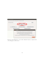
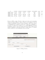
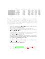
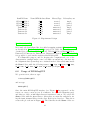
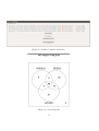
Finally, we compare the results by clicking on Result Comparison Interface.
We fill all the fields as shown in Figure 45. We click on VennDiagrams3setsDE
button. This action creates two files. The first file is the pdf shown in
Figure 46 and saved in Plots folder. The second file is a text file, called
NOISEQ DESEQ EDGER genes in intersection.txt and saved in the Results
folder. This text file reports the 86 gene-ids that fall in the intersection of
all the three methods (see in Figure 46).
All the functionalities we have used are automatically saved in a report
file inside the Logs directory.
51
Figure 44: Fold Change Plot generated by using the function PlotFC of
EdgeR
52
Figure 45: Result Comparison Interface
Figure 46: Venn Diagram
53
7
How to customize RNASeqGUI
It is extremely easy to add new buttons that calls new functions. Hence, a
user can customize RNASeqGUI interfaces for his purposes and benefits by
adding the methods he needs mostly.
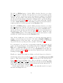
7.1
Adding a new button in just three steps
For the sake of example, suppose you have written a function that generates
a heat-map as the one written below.
MyHeatmap <- function(x,geneNum){
require(RColorBrewer)
n <- as.numeric(geneNum)
x <- as.matrix(x)
means=rowMeans(x)
select = order(means, decreasing=TRUE)[1:n]
# show first n genes
hmcol = colorRampPalette(brewer.pal(7,"Greens"))(100)
heatmap(x[select,],col=hmcol,margins=c(5,8),main="MyHeatMap")
}
If you want to add MyHeatmap function to RNASeqGUI, follow these tree
simple steps.
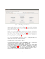
1 - Place MyHeatmap function in a file (for instance, called MyHeatmap.R)
in the R folder inside the RNASeqGUI 0.0.4 directory.
2 - Open calculateGUI1.R file (This is the file that generates the Data Exploration Interface) and copy the following 3 lines and paste them at the
bottom of this file before “}” parenthesis.
#Here you create the button, called "MY OWN FUNCTION"
MYOWNBUTTON <- gtkButtonNewWithMnemonic("MY OWN FUNCTION", show = TRUE)
#Associate the button to MyHeatmapConn that calls MyHeatmap function
gSignalConnect(MYOWNBUTTON , "clicked", MyHeatmapConn)
the.buttons$packStart(MYOWNBUTTON,fill=F)
3 - Finally, Copy the following code
MyHeatmapConn<- function(button, user.data) {
res <- NULL
# Get the information about data and the file
the.file <- filename$getText()
the.sep <- sepEntry$getText()
the.headers <- headersEntry$active
the.geneNum <- geneNum$getText()
d <- read.table(the.file,sep=the.sep,header=the.headers,row.names=1)
# Select numerical variables
numVar <- sapply(1:ncol(d),function(x){is.numeric(d[,x])})
if (sum(numVar)==0) { error <- "ERROR: No numerical variables in the data!"
}else{res=MyHeatmap(d,the.geneNum)} #HERE YOU CALL THE FUNCTION YOU DEFINED!
}
54
Figure 47: A new button called MY OWN FUNCTION is created
and paste it before the two following lines below that are written inside the
calculateGUI1.R file.
# Create window
window <- gtkWindow()
At this point, MY OWN FUNCTION button is created and the result is the one
shown in Figure 47. By clicking this button, we call MyHeatmapConn function
that calls MyHeatmap function defined before.
55
Figure 48: Session Info
8
Technical Details
To see the versions of the used methods, we type
sessionInfo()
and we get the list shown in Figure 48.
56
Acknowledgement
We want to thank M. Franzese, V. Costa and R. Esposito for suggestions
and discussions, D. Granata for technical support.
This work was supported by the Italian Flagship InterOmics Project (PB.P05)
and by BMBS COST Action BM1006.
57
References
[Anders et al., 2010] Anders,S., Huber,W. (2010) Differential expression
analysis for sequence count data. Genome Biology, 11, R106.
[Anders et al., 2013] Anders,S., McCarthy,D.J., Chen,Y., Okoniewski,M.,
Smyth, G.K., Huber,W. and Robinson,M.D. (2013) Count-based differential expression analysis of RNA sequencing data using R and
Bioconductor. Nature Protocols, 8, 1765-1786.
[Angelini et al., 2008] Angelini,C., Cutillo,L., De Canditiis,D., Mutarelli,M.,
Pensky,M. (2008) BATS: a Bayesian user-friendly software for analyzing time series microarray experiments. BMC Bioinformatics 9:415.
[Bolstad et al., 2003] Bolstad B.M., Irizarry,R.A., Astrand,M., SpeedT.P.
(2003) A Comparison of Normalization Methods for High Density
Oligonucleotide Array Data Based on Bias and Variance. Bioinformatics, 19(2), 185-193.
[Brooks et al., 2011] Brooks,A.N., Yang,L., Duff,M.O., Hansen,K.D.,
Park,J.W., Dudoit,S., Brenner,S.E., Graveley,B.R. (2011) Conservation of an RNA regulatory map between Drosophila and mammals.
Genome Research, 21, 193-202.
[Bullard et al., 2010] Bullard,J.H., Purdom, E., Hansen, K.D., Dudoit, S.
(2010) Evaluation of statistical methods for normalization and differential expression in mRNA-seq experiments. BMC Bioinformatics,
11, 94.
[Hardcastle et al., 2010] Hardcastle,T.J., Kelly,K.A. (2010) baySeq: Empirical Bayesian methods for identifying differential expression in sequence count data. Bioinformatics, 11, 422.
[Kim et al., 2013] Kim,D., Pertea,G., Trapnell,C., Pimentel,H., Kelley,R.,
SalzbergS.L .(2013) TopHat2: accurate alignment of transcriptomes
in the presence of insertions, deletions and gene fusions. Genome
Biology, 14, R36.
[Lawrence et al., 2010] Lawrence,M., Temple Lang,D. (2010) RGtk2: A
Graphical User Interface Toolkit for R. Journal of Statistical Software, 37(8).
[Lawrence et al., 2013] Lawrence,M., Huber,W., Pags,H., Aboyoun,P., Carlson M. (2013) Software for Computing and Annotating Genomic
Ranges. PLoS Comput Biol 9(8)
58
[Lohse et al., 2012] Lohse,M.,
Bolger,A.M.,
Nagel,A.,
Fernie,A.R.,
Lunn,J.E., Stitt M., Usadel B. (2012) RobiNA: a user-friendly,
integrated software solution for RNASeq-based transcriptomics.
Nucleic Acid Research, 40(W1), W622-W627.
[McCarthy et al., 2012] McCarthy,D.J., Chen,Y., Smyth,G.K. (2012) Differential expression analysis of multifactor RNA-Seq experiments with
respect to biological variation. Nucleic Acids Research, 40, 42884297.
[Morgan et al., 2014] Morgan,M., Carey,V., Lawrence,M. (2014) BiocParallel: Bioconductor facilities for parallel evaluation. R package version
0.4.1.
[Mortazavi et al., 2008] Mortazavi, A., Williams, B.A., McCue, K., Schaeffer, L., Wold, B. (2008) Mapping and quantifying mammalian transcriptomes by RNA-seq. Nature Methods, 5, 621-8.
[Pramana et al., 2013] Pramana,S. (2013) neaGUI: An R package to perform
the network enrichment analysis (NEA). R package version 1.0.0.
[Risso et al., 2011] Risso,D., Schwartz,K., Sherlock,G., Dudoit S. (2011) GCContent Normalization for RNA-Seq Data. BMC Bioinformatics, 12,
1-480.
[Robinson et al., 2010] Robinson,M.D., McCarthy,D.J., Smyth,G.K. (2010)
edgeR: a Bioconductor package for differential expression analysis of
digital gene expression data. Bioinformatics, 26, 139-140.
[Robinson et al., 2007] Robinson,M.D., McCarthy,D.J., Smyth,G.K. (2007)
Moderated statistical tests for assessing differences in tag abundance.
Bioinformatics, 23, 2881-2887.
[Robinson et al., 2008] Robinson,M.D., McCarthy,D.J., Smyth,G.K. (2008)
Small-sample estimation of negative binomial dispersion, with applications to SAGE data. Biostatistics, 9, 321-332.
[Robinson et al., 2010] Robinson,M.D., Oshlack,A. (2010) A scaling normalization method for differential expression analysis of RNA-seq data.
Genome Biology, 11, R25.
[Sanges et al., 2007] Sanges,R., Cordero,F., Calogero,R.A. (2007) oneChannelGUI: a graphical interface to Bioconductor tools, designed for life
scientists who are not familiar with R language. Bioinformatics, 23,
3406-3408.
59
[Smyth et al., 2005] Smyth,G.K. (2005) Limma: linear models for microarray data. Bioinformatics and Computational Biology Solutions using
R and Bioconductor. Springer, 397-420.
[Soneson et al., 2013] Soneson,C., Delorenzi,M. (2013) A comparison of
methods for differential expression analysis of RNA-seq data. BMC
Bioinformatics , 14, e91.
[Tarazona et al., 2011] Tarazona,S., Garcia-Alcalde,F., Ferrer,A., Dopazo,J.,
Conesa,A. (2011) Differential expression in RNA-seq: a matter of
depth. Genome Research, 21, 2213-222.
[Villa-Vialaneix et al., 2013] Villa-Vialaneix,N., Leroux,D. (2013) sexy-rgtk:
a package for programming RGtk2 GUI in a user-friendly manner.
In Proceedings of: 2mes rencontres R.
[Wettenhall et al., 2006] Wettenhall,J.M., Simpson,K.M., Satterley,K.,
Smyth,G.K. (2006) affylmGUI: a graphical user interface for linear modeling of single channel microarray data. Bioinformatics
22:897-899.
[Wettenhall et al., 2004] Wettenhall,J.M., Smyth,G.K. (2004) limmaGUI: a
graphical user interface for linear modeling of microarray data. Bioinformatics, 20, 3705-3706.
60