Download QoRTs Package User Manual

QoRTs Package User Manual
Stephen Hartley
National Human Genome Research Institute
National Institutes of Health
v0.3.5
May 22, 2015
Contents
1 Overview
3
2 Requirements
2.1 Recommendations . . . . . . . . . . . . . . . . . . . . . . . . . . . . . . . . . . . . .
4
4
3 Preparations
3.1 Alignment . . . . . . . . . . . . . . . . . . . . . . . . . . . . . . . . . . . . . . . . .
3.2 Sorting . . . . . . . . . . . . . . . . . . . . . . . . . . . . . . . . . . . . . . . . . . .
5
5
5
4 Quick Start
6
5 Dataset Organization
5.1 Example data . . . . . . . . . . . . . . . . . . . . . . . . . . . . . . . . . . . . . . .
6
7
6 Processing of aligned RNA-Seq data
8
6.1 Memory Usage . . . . . . . . . . . . . . . . . . . . . . . . . . . . . . . . . . . . . . . 10
7 Visualization
7.1 Reading the QC data into R . . . . . . . .
7.2 Generating all default plots . . . . . . . .
7.3 Plotting by sample, lane, or group . . . . .
7.3.1 Summary Plots . . . . . . . . . . .
7.3.2 Colored by Sample . . . . . . . . .
7.3.3 Colored by Lane/Batch . . . . . .
7.3.4 Colored by Group/Phenotype . . .
7.3.5 Basic Sample Highlight . . . . . .
7.3.6 Sample Highlight, Colored by Lane
7.4 Description of Individual Plots . . . . . . .
1
.
.
.
.
.
.
.
.
.
.
.
.
.
.
.
.
.
.
.
.
.
.
.
.
.
.
.
.
.
.
.
.
.
.
.
.
.
.
.
.
.
.
.
.
.
.
.
.
.
.
.
.
.
.
.
.
.
.
.
.
.
.
.
.
.
.
.
.
.
.
.
.
.
.
.
.
.
.
.
.
.
.
.
.
.
.
.
.
.
.
.
.
.
.
.
.
.
.
.
.
.
.
.
.
.
.
.
.
.
.
.
.
.
.
.
.
.
.
.
.
.
.
.
.
.
.
.
.
.
.
.
.
.
.
.
.
.
.
.
.
.
.
.
.
.
.
.
.
.
.
.
.
.
.
.
.
.
.
.
.
.
.
.
.
.
.
.
.
.
.
.
.
.
.
.
.
.
.
.
.
.
.
.
.
.
.
.
.
.
.
.
.
.
.
.
.
.
.
.
.
.
.
.
.
.
.
.
.
.
.
.
.
.
.
.
.
.
.
.
.
.
.
.
.
.
.
.
.
.
.
.
.
.
.
.
.
.
.
.
.
10
11
11
12
12
15
16
17
18
19
20
QoRTs Package User Manual
7.4.1
7.4.2
7.4.3
7.4.4
7.4.5
7.4.6
7.4.7
7.4.8
7.4.9
7.4.10
7.4.11
7.4.12
7.4.13
7.4.14
7.4.15
7.4.16
7.4.17
7.4.18
7.4.19
7.4.20
7.4.21
7.4.22
7.4.23
7.4.24
7.4.25
2
Phred Quality Score . . . . . . . . . . . . . . . . .
GC Content . . . . . . . . . . . . . . . . . . . . .
Clipping Profile . . . . . . . . . . . . . . . . . . .
Cigar Op Profile . . . . . . . . . . . . . . . . . . .
Cigar Length Distribution . . . . . . . . . . . . . .
Insert Size . . . . . . . . . . . . . . . . . . . . . .
N-Rate . . . . . . . . . . . . . . . . . . . . . . . .
Gene-Body Coverage . . . . . . . . . . . . . . . . .
Cumulative Gene Diversity . . . . . . . . . . . . . .
Nucleotide Rates, by Cycle . . . . . . . . . . . . .
Aligned Nucleotide Rates, by Cycle . . . . . . . . .
Leading Clipped Nucleotide Rates . . . . . . . . . .
Trailing Clipped Nucleotide Rates . . . . . . . . . .
Mapping location rates . . . . . . . . . . . . . . .
Splice Junction Loci . . . . . . . . . . . . . . . . .
Number of Splice Junction Events . . . . . . . . . .
Splice Junction Event Rates per Read-Pair . . . . .
Breakdown of Splice Junction Events . . . . . . . .
Breakdown of Splice Junction Events, by locus type
Strandedness test . . . . . . . . . . . . . . . . . .
Mapping stats . . . . . . . . . . . . . . . . . . . .
Chromosome counts . . . . . . . . . . . . . . . . .
Normalization Factors . . . . . . . . . . . . . . . .
Normalization Factor Ratio . . . . . . . . . . . . .
Read drop rate . . . . . . . . . . . . . . . . . . . .
.
.
.
.
.
.
.
.
.
.
.
.
.
.
.
.
.
.
.
.
.
.
.
.
.
.
.
.
.
.
.
.
.
.
.
.
.
.
.
.
.
.
.
.
.
.
.
.
.
.
.
.
.
.
.
.
.
.
.
.
.
.
.
.
.
.
.
.
.
.
.
.
.
.
.
.
.
.
.
.
.
.
.
.
.
.
.
.
.
.
.
.
.
.
.
.
.
.
.
.
.
.
.
.
.
.
.
.
.
.
.
.
.
.
.
.
.
.
.
.
.
.
.
.
.
.
.
.
.
.
.
.
.
.
.
.
.
.
.
.
.
.
.
.
.
.
.
.
.
.
.
.
.
.
.
.
.
.
.
.
.
.
.
.
.
.
.
.
.
.
.
.
.
.
.
.
.
.
.
.
.
.
.
.
.
.
.
.
.
.
.
.
.
.
.
.
.
.
.
.
.
.
.
.
.
.
.
.
.
.
.
.
.
.
.
.
.
.
.
.
.
.
.
.
.
.
.
.
.
.
.
.
.
.
.
.
.
.
.
.
.
.
.
.
.
.
.
.
.
.
.
.
.
.
.
.
.
.
.
.
.
.
.
.
.
.
.
.
.
.
.
.
.
.
.
.
.
.
.
.
.
.
.
.
.
.
.
.
.
.
.
.
.
.
.
.
.
.
.
.
.
.
.
.
.
.
.
.
.
.
.
.
.
.
.
.
.
.
.
.
.
.
.
.
.
.
.
.
.
.
.
.
.
.
.
.
.
.
.
.
.
.
.
.
.
.
.
.
.
.
.
.
.
.
.
.
.
.
.
.
.
.
.
.
.
.
.
.
.
.
.
.
.
.
.
21
22
23
24
25
26
27
28
29
30
31
32
33
34
35
36
37
38
39
40
41
42
43
44
45
8 Identifying Problems
46
8.1 Example 1: Sequencer Hiccup . . . . . . . . . . . . . . . . . . . . . . . . . . . . . . . 47
8.2 Example 2: Badly Degraded RNA . . . . . . . . . . . . . . . . . . . . . . . . . . . . . 48
9 Secondary Utilities
9.1 Generating a flattened annotation file . .
9.2 Merging Count Data . . . . . . . . . . .
9.3 Generating genome browser tracks . . . .
9.3.1 Generating wiggle tracks . . . . .
9.3.2 Merging wiggle tracks . . . . . .
9.3.3 Generating splice-junction tracks
9.3.4 Merging splice-junction tracks . .
9.4 Importing data into other tools . . . . .
9.4.1 DEXSeq compatibility . . . . . .
.
.
.
.
.
.
.
.
.
.
.
.
.
.
.
.
.
.
.
.
.
.
.
.
.
.
.
.
.
.
.
.
.
.
.
.
.
.
.
.
.
.
.
.
.
.
.
.
.
.
.
.
.
.
.
.
.
.
.
.
.
.
.
.
.
.
.
.
.
.
.
.
.
.
.
.
.
.
.
.
.
.
.
.
.
.
.
.
.
.
.
.
.
.
.
.
.
.
.
.
.
.
.
.
.
.
.
.
.
.
.
.
.
.
.
.
.
.
.
.
.
.
.
.
.
.
.
.
.
.
.
.
.
.
.
.
.
.
.
.
.
.
.
.
.
.
.
.
.
.
.
.
.
.
.
.
.
.
.
.
.
.
.
.
.
.
.
.
.
.
.
.
.
.
.
.
.
.
.
.
.
.
.
.
.
.
.
.
.
.
.
.
.
.
.
.
.
.
.
.
.
.
.
.
.
.
.
.
.
.
.
.
.
.
.
.
.
.
.
.
.
.
.
.
.
50
50
50
51
51
53
53
54
55
55
10 Session Information
56
11 Legal
57
QoRTs Package User Manual
1
3
Overview
The QoRTs software package is a fast, efficient, and portable multifunction toolkit designed to assist in
the analysis, quality control, and data management of RNA-Seq datasets. Its primary function is to aid
in the detection and identification of errors, biases, and artifacts produced by paired-end high-throughput
RNA-Seq technology. In addition, it can produce count data designed for use with differential expression
1
and differential exon usage tools 2 , as well as individual-sample and/or group-summary genome track
files suitable for use with the UCSC genome browser (or any compatible browser).
In its primary role as a QC tool it can produce a wide variety of graphs, plots, and tables that allow
the data to be visualized in various ways. Data can be compiled and contrasted in multiple ways to
allow systematic errors or artifacts to reveal themselves more easily. While it will not directly assign
pass/fail status, it is a powerful tool for bioinformaticians to detect and identify features in the data.
In (hopefully) most cases, these plots and graphs will not reveal anything other than mixed statistical
noise. Next-Gen sequencing technologies have matured to the point where gross systematic errors and
batch-specific biases are relatively modest and rare. However: mistakes can still occur, and basing
conclusions on flawed data can be disastrous.
Across the field of bioinformatics there are numerous cases where biases, artifacts, and other data
quality or bioinformatic issues have called results into question, sometimes resulting in retractions. In
many of these cases the problems were only identified after the study came under intense scrutiny
when the results were interesting and/or contentious, and the specific issues at fault were generally not
well-characterized until afterwards. The primary purpose of QoRTs is to cast a wide net, characterizing
the data in as many ways as is feasible so that quality issues that would otherwise be obscured can be
recognized and dealt with, even if these issues have not been previously encountered.
The QoRTs package is composed of two parts: a java jar-file (for data processing) and a companion R
package (for generating tables, figures, and plots). The java utility is written in the Scala programming
language (v2.11.1), however, it has been compiled to java byte-code and does not require an installation
of Scala (or any other external libraries) in order to function. The entire QoRTs toolkit can be used
on almost any operating system that supports java and R. While not explicitly required, the use of a
64-bit version of java is recommended.
This vignette primarily covers the quality control functionality of QoRTs, and briefly covers the other
functions and capabilities.
The most recent release of QoRTs is available on the QoRTs github page (http://github.com/
hartleys/QoRTs). Additional help and documentation is available online (http://hartleys.github.
io/QoRTs/index.html). A comprehensive walkthrough covering the entire process from post-alignment
all the way to differential expression analysis, along with a full example dataset and example output can be found online (https://dl.dropboxusercontent.com/u/103621176/qorts/exData/
QoRTsFullExampleData.zip).
1
2
Such as DESeq, DESeq2 [1] or edgeR [2]
Such as DEXSeq [3]
QoRTs Package User Manual
2
4
Requirements
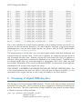
Hardware: The java utility performs the bulk of the data processing, and will generally require at least
4gb of RAM. In general at least 8gb is recommended if available. The R package is only responsible for some light data processing and for plotting/visualization, and thus has much lower resource
requirements. It should run adequately on any reasonably-powerful workstation.
Software: The QoRTs software package requires R version 3.0.2 or higher, as well as java 6 or higher.
It is strongly recommended that a 64-bit version of java be used, as the 32-bit versions generally cannot
allocate sufficient RAM.
Annotation: QoRTs requires transcript annotations in the form of a gtf file. If you are using a
annotation-guided aligner (which is STRONGLY recommended) it is likely you already have a transcript
gtf file for your reference genome. We recommend you use the same annotation gtf for alignment, QC,
and downstream analysis. We have found the Ensembl ”Gene Sets” gtf3 suitable for these purposes.
However, any format that adheres to the gtf file specification4 will work.
Dataset: QoRTs requires aligned RNA-Seq data. Data can be paired-end or single-end, unstranded or
stranded (using either strandedness rule, see Section 6). It is strongly recommended, but not explicitly
required, that the SAM/BAM files be sorted (either by name or position). QoRTs can use additional
metadata (such as technical replicate status, case/control status, batch id, etc) to produce comparisons
between these replicate groups, but this information is optional.
2.1
Recommendations
Clipping: For the purposes of Quality Control, it is generally best if reads are NOT hard-clipped prior to
alignment. This is because hard clipping, espeically variable hard-clipping from both the start and end
of reads, makes it impossible to determine sequencer cycle from the aligned bam files, which in turn can
obfuscate cycle specific artifacts, biases, errors, and effects. If undesired sequence must be removed,
it is generally preferred to replace such nucleotides with N’s, as this preserves cycle information. Note
that many advanced RNA-Seq aligners will ”soft clip” nonmatching sequence that occurs on the read
ends, so hard-clipping low quality sequence is generally unnessessary and may reduce mapping rate and
accuracy.
Replicates: Using barcoding, it is possible to build a combined library of multiple distinct samples which
can be run together on the sequencing machine and then demultiplexed afterward. In general, it is
recommended that samples for a particular study be multiplexed and merged into ”balanced” combined
libraries, each containing equal numbers of each biological condition. If necessary, these combined
libraries can be run across multiple sequencer lanes or runs to achieve the desired read depth on each
sample.
3
4
Which can be acquired from the Ensembl website at http://www.ensembl.org
See the gtf file specification at http://genome.ucsc.edu/FAQ/FAQformat.html
QoRTs Package User Manual
3
5
Preparations
There are a number of processing steps that must occur prior to the creation of usable bam files. We
will briefly go over the required steps here:
3.1
Alignment
QoRTs is designed to run on paired-ended or single-ended next-gen RNA-Seq data. The data must be
aligned (or ”mapped”) to a reference genome before QoRTs can be run. RNA-Star [4], GSNAP [5],
and TopHat2 [6] are all popular and effective aligners for use with RNA-Seq data. The use of short-read
or unspliced aligners such as BowTie, ELAND, BWA, or Novoalign is NOT recommended.
3.2
Sorting
For single-end data, the reads can be in any order, and sorting is unnecessary.
For paired-end data, QoRTs is designed to automatically accept files sorted by either read-name or
position. Sorting can be accomplished via the samtools or novosort tools (which are NOT included with
QoRTs). Sorting is unnecessary for single-end data.
To sort by coordinate:
samtools sort unsorted.bam sorted
OR
novosort unsorted.bam > sorted.bam
Or, to sort by read name:
samtools sort -n unsorted.bam sortedByName
OR
novosort -n unsorted.bam > sortedByName.bam
Running in the default mode, QoRTs will accept both name-sorted and position-sorted BAM files.
Technically QoRTs can accept any BAM files regardless of ordering; however, if a large number of
paired mates are not located near one another in the file then memory usage may be too high as
QoRTs stores unmatched mates in memory.
QoRTs also has a separate mode designed only for name-sorted samples, which can be activated using
the ”--nameSorted” option. Under certain conditions this may improve speed and reduce memory
usage. Under typical conditions any improvement is trivial.
QoRTs Package User Manual
4
6
Quick Start
In order to produce quality control metrics, plots, and pdf reports on a single replicate, simply use the
command:
java -Xmx4G -jar /path/to/jarfile/QoRTs.jar QC \
--generatePlots \
mybamfile.bam \
transcriptAnnotationFile.gtf.gz
/qc/data/dir/path/
\
Note: This command must be executed as a single line. Additional options may be required depending on the nature of the dataset. For single-ended data, the --singleEnded option should be
included. For strand-specific data, the --stranded option should be included, and possibly also the
--fr_secondStrand option depending on the stranded library type. For position-sorted data, the
--coordSorted option should be used. See 6, or the QC utility documentation5 for more information
on the available options.
5
Dataset Organization
Several QoRTs functions will require ”decoder” information in some form, which describes each sample
and all of its technical replicates (if any). The simplest method is to provide a decoder file. All of the
columns are optional except for unique.ID, however if group, lane, and/or technical replicate information
is not supplied then QoRTs obviously will not be able to produce plots that organized and/or grouped
by these factors.
Fields:
ˆ unique.ID: A unique identifier for the row. QoRTs will also accept the synonym ”lanebam.ID”.
THIS IS THE ONLY MANDATORY FIELD.
ˆ lane.ID: The ID of the lane or batch. By default this will be set to ”UNKNOWN”.
ˆ group.ID: The ID of the ”group”. For example: ”Case” or ”Control”. By default this will be set
to ”UNKNOWN”.
ˆ sample.ID: The ID of the biological sample from which the data originated. Each sample can
have multiple rows, representing technical replicates (in which the same sample is sequenced on
multiple lanes or runs). By default QoRTs will assume that every row comes from a separate
sample, and will thus set the sample.ID to equal the unique.ID.
ˆ qc.data.dir : The directory in which the java utility saved all the output data. If this column does
not exist, by default it will be set to be unique.ID.
ˆ input.read.pair.count: (Optional) The number of reads in the original fastq file, prior to alignment.
If this field is left out, then QoRTs will skip comparisons and plotting of mapping rates. There
are a number of other ways to input this value. See Section 7.4.21.
5
Found here.
QoRTs Package User Manual
7
ˆ multi.mapped.read.pair.count: (Optional) The number of reads that were multi-mapped by the
aligner. This field should only be used if filtering for multi-mapped reads is performed prior to
analysis with QoRTs (which is not recommended). Even in this case, this field can simply be left
out and QoRTs will skip plotting and comparisons of multi-mapping rates. See Section 7.4.21.
In addition, the decoder can contain any other additional columns as desired, as long as all of the
column names are distinct.
While QoRTs is primarily designed to allow comparisons between biological groups, lanes, sequencingruns, etc, it can also be used on simpler datasets, or even individual samples. Thus, only the unique.ID
variable is actually required. For testing purposes, you can produce a completed decoder (with all
default values filled in) using the completeAndCheckDecoder function.
The simplest example would just be a character vector of unique.ID’s:
completeAndCheckDecoder(c("SAMPLE1","SAMPLE2","SAMPLE3"));
##
unique.ID sample.ID lane.ID group.ID qc.data.dir
## 1
SAMPLE1
SAMPLE1 UNKNOWN UNKNOWN
SAMPLE1
## 2
SAMPLE2
SAMPLE2 UNKNOWN UNKNOWN
SAMPLE2
## 3
SAMPLE3
SAMPLE3 UNKNOWN UNKNOWN
SAMPLE3
Alternatively, any of the optional fields can be included or left out, as desired:
incompleteDecoder <- data.frame(unique.ID = c("SAMPLE1", "SAMPLE2"),
group.ID = c("CASE","CONTROL"));
completeAndCheckDecoder(incompleteDecoder);
##
unique.ID group.ID sample.ID lane.ID qc.data.dir
## 1
SAMPLE1
CASE
SAMPLE1 UNKNOWN
SAMPLE1
## 2
SAMPLE2 CONTROL
SAMPLE2 UNKNOWN
SAMPLE2
5.1
Example data
The separate R package QoRTsExampleData contains an example dataset with an example decoder:
directory <- system.file("extdata/", package="QoRTsExampleData",
mustWork=TRUE);
decoder.file <- system.file("extdata/decoder.txt",
package="QoRTsExampleData",
mustWork=TRUE);
decoder.data <- read.table(decoder.file,
header=T,
stringsAsFactors=F);
print(decoder.data);
##
## 1
## 2
sample.ID lane.ID unique.ID qc.data.dir group.ID input.read.pair.count
SAMP1
L1 SAMP1_RG1 ex/SAMP1_RG1
CASE
465298
SAMP1
L2 SAMP1_RG2 ex/SAMP1_RG2
CASE
472241
QoRTs Package User Manual
##
##
##
##
##
##
##
##
##
##
##
##
##
##
##
##
3
4
5
6
7
8
9
10
11
12
13
14
15
16
17
18
SAMP1
SAMP2
SAMP2
SAMP2
SAMP3
SAMP3
SAMP3
SAMP4
SAMP4
SAMP4
SAMP5
SAMP5
SAMP5
SAMP6
SAMP6
SAMP6
L3
L1
L2
L3
L1
L2
L3
L1
L2
L3
L1
L2
L3
L1
L2
L3
8
SAMP1_RG3
SAMP2_RG1
SAMP2_RG2
SAMP2_RG3
SAMP3_RG1
SAMP3_RG2
SAMP3_RG3
SAMP4_RG1
SAMP4_RG2
SAMP4_RG3
SAMP5_RG1
SAMP5_RG2
SAMP5_RG3
SAMP6_RG1
SAMP6_RG2
SAMP6_RG3
ex/SAMP1_RG3
ex/SAMP2_RG1
ex/SAMP2_RG2
ex/SAMP2_RG3
ex/SAMP3_RG1
ex/SAMP3_RG2
ex/SAMP3_RG3
ex/SAMP4_RG1
ex/SAMP4_RG2
ex/SAMP4_RG3
ex/SAMP5_RG1
ex/SAMP5_RG2
ex/SAMP5_RG3
ex/SAMP6_RG1
ex/SAMP6_RG2
ex/SAMP6_RG3
CASE
CASE
CASE
CASE
CASE
CASE
CASE
CTRL
CTRL
CTRL
CTRL
CTRL
CTRL
CTRL
CTRL
CTRL
500691
461405
467713
492322
485397
489859
516906
460968
468391
484530
469884
475001
494213
452429
458810
477751
Due to size constraints the example dataset contained in this R package includes only the QC output data, not the raw bam-files themselves. The actual bamfiles, along with a step-by-step example
walkthrough that covers the entire analysis pipeline, are linked to from the QoRTs github website
(https://github.com/hartleys/QoRTs).
The example dataset is derived from a set of rat pineal gland samples, which were multiplexed and
sequenced across six sequencer lanes. For the sake of simplicity, the example dataset was limited to
only six samples and three lanes. However, the bam files alone would still occupy 18 gigabytes of
disk space, which would make it unsuitable for distribution as an example dataset. To further reduce
the example bamfile sizes, only reads that mapped to chromosomes chr14, chr15, chrX, and chrM
were included. Additionally, all the selected chromosomes EXCEPT for chromosome 14 were randomly
downsampled to 30 percent of their original read counts.
THIS DATASET IS INTENDED FOR DEMONSTRATION AND TESTING PURPOSES ONLY. Due
to the various alterations that have been made to reduce file sizes and improve portability, it is not
representitive of the original data and as such is really not suitable for any actual analyses.
6
Processing of aligned RNA-Seq data
The first step is to process the aligned RNA-Seq data. The bulk of the data-processing is performed
by the QoRTs.jar java utility. This tool produces an array of output files, analyzing and tabulating the
data in various ways. This utility requires about 10-20gb of RAM for most genomes, and takes roughly
4-7 minutes to process 1 million read-pairs.
java -jar /path/to/jarfile/QoRTs.jar QC \
mybamfile.bam \
transcriptAnnotationFile.gtf.gz \
QoRTs Package User Manual
9
/qc/data/dir/path/
In the above command (which must be entered as a single line), you must replace /path/to/jarfile/
with the file-path to the directory in which the jar file is kept. The path /qc/data/dir/path/ should
be replaced with the path you want the QC data to be written. This should match the path located in
the decoder in the qc.data.dir column for this sample-run.
The bam processing tool includes numerous options. A full description of these options can be found
in the online documentation of the jar utility6 , or by entering the command:
java -jar /path/to/jarfile/QoRTs.jar QC --man
There are a number of crucial points that require attention when using the QoRTs.jar QC command.
ˆ Stranded Data: By default, QoRTs assumes that the data is NOT strand-specific. For strandspecific data, the --stranded option must be used.
ˆ Stranded Library Type: The --fr_secondStrand option may be required depending on the
stranded library type. QoRTs does not attempt to automatically detect the platform and protocol used for stranded data. There are two types of strand-specific protocols, which are described
by the TopHat/CuffLinks documentation at http://cufflinks.cbcb.umd.edu/manual.html#
library as fr-firststrand and fr-secondstrand. In HTSeq, these same library type options are defined as -s reverse and -s yes respectively. According to the CuffLinks manual,
fr-firststrand (the default used by QoRTs for stranded data) applies to dUTP, NSR, and
NNSR protocols, whereas fr-secondstrand applies to ”Directional Illumina (ligation)” and
”Standard SOLiD” protocols. If you are unsure which library type applies to your dataset, don’t
worry: one of the tests will report stranded library type. If you use this test to determine library
type, be aware that you may have to re-run QoRTs with the correct library type set.
ˆ Read Groups: Depending on the production pipeline, each biological sample may be run across
multiple sequencer lanes. These seperate files can be merged together either before or after
analysis with QoRTs (and maybe even before alignment). However, if the merger occurs before
analysis with QoRTs, then each bam file will consist of multiple seperate lanes or runs. In this
case, it is STRONGLY recommended that seperate QC runs be performed on each ”read group”,
using the --readGroup option. This will prevent run- or lane-specific biases, artifacts, or errors
from being obfuscated.
ˆ Read Sorting: For paired-end data reads must be sorted. By default, QoRTs can accept files
sorted by name OR by position.
ˆ Single-end vs paired-end: By default, QoRTs assumes the input bam file consists of paired-end
data. For single-end data, the --isSingleEnd option must be used.
For example, to read the first read group bam-file for SAMP1 from the example dataset (which is
stranded, coordinate-sorted, and uses the fr_firstStrand stranded library type), one would use the
following command:
java -jar /path/to/jarfile/QoRTs.jar QC \
--stranded \
inputData/bamFiles/SAMP1_RG1.bam \
inputData/annoFiles/anno.gtf.gz \
6
Found here: http://hartleys.github.io/QoRTs/jarHtml/index.html
QoRTs Package User Manual
10
outputData/qortsData/SAMP1_RG1/
This command must be run on each bam file (and possibly more than once on each, if each bam file
consists of multiple separate read-groups).
6.1
Memory Usage
Memory usage: The QoRTs QC utility requires at least 4gb or RAM for most genomes / datasets.
Larger genomes, genomes with more annotated genes/transcripts, or larger bam files may require more
RAM. You can set the maximum amount of RAM allocated to the JVM using the options -Xmx4000M.
This should be included before the -jar in the command line. For example:
#Set the maximum to the minimum recommended 4 gigabytes:
java -Xmx4000M -jar /path/to/jarfile/QoRTs.jar QC \
--stranded \
inputData/bamFiles/SAMP1_RG1.bam \
inputData/annoFiles/anno.gtf.gz \
outputData/qortsData/SAMP1_RG1/
#Or Set the maximum to 16 gigabytes:
java -Xmx16G -jar /path/to/jarfile/QoRTs.jar QC \
--stranded \
inputData/bamFiles/SAMP1_RG1.bam \
inputData/annoFiles/anno.gtf.gz \
outputData/qortsData/SAMP1_RG1/
This option can be used with any and all of the QoRTs java utilities.
7
Visualization
All visualization is performed the the QoRTs companion R package.
For basic QC analyses it is often not necessary to write any R code, as QoRTs comes with a simple R
script that generates a standard set of png multiplots, pdf reports, and a large tab-delimited summary
table. The qortsGenMultiQC.R script should be included in the scripts directory of the main package
archive. This script can be run using the command:
Rscript qortsGenMultiQC.R infile/dir/ decoderFile.txt outfile/dir/
infile/dir/ should be the parent directory within which all the QC output data is contained.
decoderFile.txt should be the decoder file, as described in Section 5. outfile/dir/ should be
the directory where all output plots will be placed.
Alternatively, custom R code can be used to generate non-standard plots or multiplots, alter plotting
parameters, or to generate plots interactively. In addition to the documentation provided in the rest
QoRTs Package User Manual
11
of this section, the full R docs can be found online. See the github page for a link to the complete
documentation.
7.1
Reading the QC data into R
First you must read in all the QC output from the java utility, using the command below. This command
requires 2 arguments: a root directory and a decoder (which can be either a data frame or a file). We
will be using the example data found in package QoRTexampleData, which is described in Section 5.1.
res <- read.qc.results.data(directory, decoder = decoder.data,
calc.DESeq2 = TRUE, calc.edgeR = TRUE);
Note that the calc.DESeq2 and calc.edgeR options are optional, and tell QoRTs to attempt to
load the DESeq2 and edgeR packages (respectively) and use the packages to calculate additional
normalization size factors. This is not strictly needed for most purposes, but allows QoRTs to plot the
normalization factors against one another. See section 7.4.23 for more information.
7.2
Generating all default plots
To generate all the default compiled plots all at once, use the command:
makeMultiPlot.all(res, outfile.dir = "./");
This will usually take some time to run, but will produce all the compiled summary plots described in
the rest of this section, including separate highlight plots for every sample in the dataset. By default
all images will saved to file as pngs. There are a number of alternatives, which can be selected using
the plot.device.name parameter. For example:
#Generate multi-page pdf reports:
makeMultiPlot.all(res, outfile.dir = "./", plot.device.name = "pdf");
#Generate svg vector drawings:
makeMultiPlot.all(res, outfile.dir = "./", plot.device.name = "svg");
Note: The R PDF device primarily uses vector drawings, however, some of the plots are too large to be
efficiently stored as vectors. If pdf reports are desired, we recommend installing the png package. If this
package is installed, then QoRTs will automatically rasterize the plotting areas of certain large plots (in
particular: the gene diversity plots and the various NVC plots). Setting the rasterize.large.plots
parameter to FALSE will deactivate this behavior. The raster.height and raster.width parameters
can be used to increase the pixel resolution of the rasterized plotting regions, if desired.
The png package can be installed with the R command:
install.packages("png");
QoRTs Package User Manual
7.3
12
Plotting by sample, lane, or group
QoRTs includes automated methods for organizing and plotting the results in numerous different ways.
The intent of these tools is to make any patterns and biases more visible to the user.
All plotting functions in QoRTs require a QoRTs Plotter object. A QoRTs Plotter is a RefClass
object that contains all the QC data along with a set of parameters that determine how to color and
draw each replicate’s data. A full accounting of all possible options available in the is beyond the scope
of this manual, but can be found in the help docs for the QoRTs Plotter class.
7.3.1
Summary Plots
The most basic QoRTs Plotter can be created using the command:
basic.plotter <- build.plotter.basic(res);
This QoRTs Plotter object can be used to plot all replicates on top of one another in semi-transparent
blue. For example:
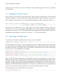
makePlot.insert.size(basic.plotter);
Which produces Figure 1:
Figure 1: Phred Quality Score Plots
The above example plot displays the ”Insert Size” of each replicate, as described in Section 7.4.6.
QoRTs Package User Manual
13
In addition, a compiled multi-plot in this style, containing all the standard QC plots, can be generated
with the command:
makeMultiPlot.basic(res);
Which produces Figure 2:
Figure 2: Compiled summary multi-plot
This plot includes many sub-plots, all in a single frame. The sub-plots are:
ˆ
ˆ
ˆ
ˆ
ˆ
ˆ
(a): Minimum phred quality score, by read position. Described in section 7.4.1
(b): Lower-quartile phred quality score, by read position. Described in section 7.4.1
(c): Median phred quality score, by read position. Described in section 7.4.1
(d): Upper-quartile phred quality score, by read position. Described in section 7.4.1
(e): Maximum phred quality score, by read position. Described in section 7.4.1
(f): Clipping profile. Described in section 7.4.3
QoRTs Package User Manual
ˆ
ˆ
ˆ
ˆ
ˆ
ˆ
ˆ
ˆ
ˆ
ˆ
ˆ
ˆ
ˆ
ˆ
ˆ
ˆ
ˆ
ˆ
ˆ
ˆ
ˆ
ˆ
ˆ
ˆ
ˆ
ˆ
14
(g): Deletion profile. Described in section 7.4.4
(h): Insertion profile. Described in section 7.4.4
(i): Splicing profile. Described in section 7.4.4
(j): Insertion length distribution. Described in section 7.4.5
(k): Deletion length distribution. Described in section 7.4.5
(l): GC content distribution. Described in section 7.4.2
(m): N-rate, by read position. Described in section 7.4.7
(n): Read drop rate. Described in section 7.4.25
(o): Insert size distribution. Described in section 7.4.6
(p): Cumulative gene assignment diversity. Described in section 7.4.9
(q): Gene body coverage, overall. Described in section 7.4.8
(r): Gene body coverage, upper-middle quartile genes. Described in section 7.4.8
(s): Gene body coverage, low expression genes. Described in section 7.4.8
(t): Read mapping location rates. Described in section 7.4.14
(u): Observed splice junction loci counts. Described in section 7.4.15
(v): Splice junction event distribution. Described in section 7.4.17
(w): Splice junction events per read-pair. Described in section 7.4.19
(x): Read-mapping statistics. Described in section 7.4.21
(y): Chromosome counts. Described in section 7.4.22
(z): Comparison of normalization factors. Described in section 7.4.23
(aa): Comparison of normalization factors relative to TC normalization. Described in section
7.4.24
(ab): Strandedness test. Described in section 7.4.20
(ac): Leading-clipped nucleotide rates. Described in section 7.4.12
(ad): Trailing-clipped nucleotide rates. Described in section 7.4.13
(ae): Raw nucleotide rate by read position. Described in section 7.4.10
(af): Aligned nucleotide rate by read position. Described in section 7.4.11
A printable pdf version of this multi-plot, with 6 plots on each page, can be generated with using the
options:
makeMultiPlot.basic(res, plot.device.name = "pdf");
QoRTs Package User Manual
7.3.2
15
Colored by Sample
For small datasets, it can be useful to simply color each sample a distinct color, so that outliers can be
easily identified. For this, you first generate a QoRTs Plotter using the command:
bySample.plotter <- build.plotter.colorBySample(res);
This QoRTs Plotter can be used to draw all the replicate on top of one another, but color them based
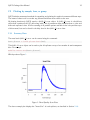
on their sample.ID. The plotter can then be used to create various QC plots, for example:
makePlot.insert.size(bySample.plotter);
makePlot.legend.over("topright",bySample.plotter);
Which produces Figure 3:
Figure 3: Phred Quality Score Plots
The above example plot displays the ”Insert Size” of each replicate, as described in Section 7.4.6.
In addition, a compiled multi-plot in this style, containing all the standard QC plots, can be generated
with the command:
makeMultiPlot.colorBySample(res);
QoRTs Package User Manual
7.3.3
16
Colored by Lane/Batch
In order to more easily detect batch effects, it is possible to color each replicate by lane/batch. For
this, you can generate a QoRTs Plotter with the command:
byLane.plotter <- build.plotter.colorByLane(res);
This QoRTs Plotter can be used to color replicates based on lane.ID. The QoRTs Plotter can then
be used to create various QC plots, for example:
makePlot.insert.size(byLane.plotter);
makePlot.legend.over("topright",byLane.plotter);
Which produces Figure 4:
Figure 4: Phred Quality Score Plots
The above example plot displays the ”Insert Size” of each replicate, as described in Section 7.4.6.
In addition, a compiled multi-plot in this style, containing all the standard QC plots, can be generated
with the command:
makeMultiPlot.colorByLane(res);
QoRTs Package User Manual
7.3.4
17
Colored by Group/Phenotype
To detect variations caused by biological conditions (or artifacts and errors that occur disproportionately
in certain biological conditions), it is sometimes useful to color samples by group.ID.
byGroup.plotter <- build.plotter.colorByGroup(res);
This QoRTs Plotter can then be used to create various QC plots, for example:
makePlot.insert.size(byGroup.plotter);
makePlot.legend.over("topright",byGroup.plotter);
Which produces Figure 5:
Figure 5: Phred Quality Score Plots
The above example plot displays the ”Insert Size” of each replicate, as described in Section 7.4.6.
In addition, a compiled multi-plot in this style, containing all the standard QC plots, can be generated
with the command:
makeMultiPlot.colorByGroup(res);
QoRTs Package User Manual
7.3.5
18
Basic Sample Highlight
Sometimes it is useful to ”highlight” an individual sample.
sample.SAMP1.plotter <- build.plotter.highlightSample("SAMP1",res);
This QoRTs Plotter can then be used to create various QC plots, for example:
makePlot.insert.size(sample.SAMP1.plotter);
makePlot.legend.over("topright",sample.SAMP1.plotter);
Which produces Figure 6:
Figure 6: Phred Quality Score Plots
The above example plot displays the ”Insert Size” of each replicate, as described in Section 7.4.6.
In addition, a compiled multi-plot in this style, containing all the standard QC plots, can be generated
with the command:
makeMultiPlot.highlightSample(res,
curr.sample = "SAMP1");
QoRTs Package User Manual
7.3.6
19
Sample Highlight, Colored by Lane
Sometimes it can be useful to highlight an individual sample. However, if that sample has multiple
”technical replicates” (derived from multiple separate lanes/runs on the same library), it can be useful
to color the different runs with different distinct colors. With this plotter, only the ”highlighted” sample
is colored, all other samples are colored Gray.
sample.SAMP1.colorByLane.plotter <build.plotter.highlightSample.colorByLane("SAMP1",res);
This QoRTs Plotter can then be used to create various QC plots, for example:
makePlot.insert.size(sample.SAMP1.colorByLane.plotter);
makePlot.legend.over("topright",sample.SAMP1.colorByLane.plotter);
Which produces Figure 7:
Figure 7: Phred Quality Score Plots
The above example plot displays the ”Insert Size” of each replicate, as described in Section 7.4.6.
In addition, a compiled multi-plot in this style, containing all the standard QC plots, can be generated
with the command:
makeMultiPlot.highlightSample.colorByLane(res,
curr.sample = "SAMP1");
QoRTs Package User Manual
7.4
20
Description of Individual Plots
QoRTs is capable of producing a wide variety of different plots and graphs. While most of these plots
will not be particularly interesting or informative in the majority of cases, they may reveal artifacts or
errors if and when they occur.
The example plots in the following section all use the byLane.plotter QoRTs Plotter (from Section
7.3.3), which colors each replicate by its lane ID.
What it means and what to look for:
In general, when examining these plots, users should scan for a number of potential anomalies:
ˆ ”Spikes”: In which one of the metrics jumps up or down abruptly, then returns to baseline.
ˆ ”Shelves”: In which one of the metrics jumps up or down abruptly, then continues at an increased
or decreased level.
ˆ Outliers: In which one or more particular samples or replicates are very different from all or most
of the others. The presence of outliers may be an indicator for sample-collection, library-prep, or
sequencing errors or artifacts.
ˆ Systematic Biases: In which consistent differences appear between subsets of the data (eg.
”lane.ID” or ”group.ID”). Many of the biases measured by QoRTs are well-characterized, and
many downstream analysis tools are robust against them when they are consistent and uniform.
However: biases that vary disproportionately between sample groups may still drive false associations downstream.
ˆ Inconsistent samples: In which the technical replicates of a specific biological sample shows substantial variation. In most studies, technical variation is very small relative to biological variation. In
the example dataset (for example) the technical replicates are plotted almost on top of one another
across many of the plots. If technical replicates do not cluster tightly, or if they cluster with the
wrong replicates, then this may be an indicator of a sample swap.
Some ”anomalous” metrics may be fundamental to the dataset and may not be indicative of any
quality issues. For example, when profiling two different cell types one would expect the two groups
to have very different profiles across a number of metrics. However: a single sample that is wildly
different from the others within the same group may be cause for concern. In many cases variations
may be observed across multiple metrics, all driven by the same underlying phenomenon. The
breadth and depth of the metrics provided are intended to provide the tools necessary to identify
the most likely underlying source(s) of the aberration(s).
Some aberrations may not be relevant to the study analysis even when they are representative of a
real data quality issue. A moderate increase in the deletion rate may not have a noticable impact
on expression quantification in a simple differential expression study. The same issue, however,
might be catastrophic in a study focused on quantifying the rate of RNA transcription errors or
RNA editing events. The number of combinations of study design, sample set structure, sequencing
technology, and observed quality control issues are myriad, and all of these factors would inform
decisionmaking.
Ultimatiely, bioinformaticians must use their own judgement in deciding how to proceed when
unexplained abnormalities are discovered in their dataset.
QoRTs Package User Manual
7.4.1
21
Phred Quality Score
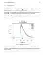
Figure 8: Phred Quality Score Plots
The plots shown in Figure 8 displays information about the phred quality score (y-axis) as a function
of the position in the read (x-axis). Five statistics can be plotted: minimum, maximum, upper and
lower quartiles, and median. These statistics are calculated individually for each replicate and each read
position (ie, each plotted line corresponds to a replicate).
Note that the Phred score is always an integer, and as such these plots would normally be very difficult
to read because lines would be plotted directly on top of one another. To reduce this problem, the plots
are vertically offset from one another.
These plots can be generated individually with the commands:
makePlot.qual.pair(byLane.plotter,"lowerQuartile");
makePlot.qual.pair(byLane.plotter,"median");
makePlot.qual.pair(byLane.plotter,"upperQuartile");
Additional options (Not shown):
makePlot.qual.pair(byLane.plotter,"min");
makePlot.qual.pair(byLane.plotter,"max");
What it means and what to look for: These plots can be used to detect sequencer problems, bad lanes, or
similar hardware-level artifacts and errors. Look for spikes or shelves, and ensure that the quality score is
relatively consistent across samples and lanes, and that any differences that do exist are not disproportionate
with respect to the study condition (or ”group.ID”).
QoRTs Package User Manual
7.4.2
22
GC Content
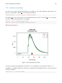
Figure 9: GC Bias
For each replicate, Figure 9 displays a histogram showing the frequency that different proportions of G
and C (versus A, T, and N) appear in the replicate’s reads. Each plotted line corresponds to a replicate.
At the bottom of the plot the mean average G/C content is also plotted. Once again, the means are
offset from one another by lane, to allow for easy detection of batch effects.
This plot can be generated individually with the command:
makePlot.gc(byLane.plotter);
The byPair option can be used to calculate the GC-distribution for read-pairs rather than for all
reads individually. This is disabled by default because it often results in a jagged distribution when a
appreciable proportion of the reads have an insert size equal to or smaller than the read length. When
this occurs, the read-pair will almost always have an even number of G/C nucleotides.
What it means and what to look for: GC bias has been indicated as a potential driver of false discoveries.
Under certain circumstances the GC bias may vary by batch or by sample. If this is apparent in your
dataset, particularly if it is associated with study conditions, one may need to apply a GC bias correction
method (such as CQN).
QoRTs Package User Manual
7.4.3
23
Clipping Profile
Figure 10: Clipping Profile
For each replicate, Figure 10 displays the rate (y-axis) at which the aligner soft-clips the reads as a
function of read position (x-axis). Note that this will only be informative when using aligners that are
capable of soft-clipped alignment (such as RNA-Star or GSNAP, but not TopHat).
This plot can be generated individually with the command:
makePlot.clipping(byLane.plotter);
What it means and what to look for: Abnormalities (”spikes”, ”shelves”, or cases where sample groups are
visibly different) in these plots can be caused by adaptor sequencing, gene fusions, mutations, population
stratification, or differences in insert size.
QoRTs Package User Manual
7.4.4
24
Cigar Op Profile
Figure 11: Cigar Operation Profiles
For each replicate, Figure 11 displays the rate (y-axis) of various cigar operations as a function of read
position (x-axis). All 9 legal cigar operations can be plotted, but for most purposes only Deletions,
Insertions, and Splice junctions will be informative.
This plot can be generated with the command:
makePlot.cigarOp.byCycle(byLane.plotter, "Del");
makePlot.cigarOp.byCycle(byLane.plotter, "Ins");
makePlot.cigarOp.byCycle(byLane.plotter, "Splice");
What it means and what to look for: These plots are most often used in conjuction with the plots in Section
7.4.5. Among other things these plots can reveal sequencer errors: a sequencer cycle-skip might result in
a spike in the deletion rate at a particular cycle, whereas an incomplete wash may result in a spike in the
insertion rate. These plots may also reveal biological differences like population stratification (eg: a subpopulation disproportionately mismatches the reference genome), or broad genome rearrangements/editing
(eg: in cancer cells).
In the example dataset, apparent spikes are plainly visible, stemming from deletions in one short and
highly-expressed mitochondrial gene. The plots are also fairly noisy due to the small number of reads used
in the example dataset and the extremely low frequency of deletions/insertions.
QoRTs Package User Manual
7.4.5
25
Cigar Length Distribution
Figure 12: Cigar Length Distribution
The plots in Figure 12 display histograms of cigar operation lengths for each replicate.
These plots can be generated individually with the commands:
makePlot.cigarLength.distribution(byLane.plotter, "Ins");
makePlot.cigarLength.distribution(byLane.plotter, "Del")
What it means and what to look for: These plots are most often used in conjuction with the plots in Section
7.4.4. They can elucidate the nature of any oddities observed in the previous plots. For example: a large
spike at one particular length may suggest that an apparent spike may be due simply to an unannotated
variant in one particular high-expression gene, although further investigation is likely merited, to confirm
that this is the case.
QoRTs Package User Manual
7.4.6
26
Insert Size
Figure 13: Insert Size
For each replicate, Figure 13 displays a histogram of the ”insert size”. Each line corresponds to one replicate,
and displays the rate (y-axis) at which that replicate’s reads possess a given insert size (x-axis).
Definition: ”Insert Size”: The ”insert size” is the length (in base-pairs) between the two sequencing adapters
for a pair of paired-end reads. In other words, it is the size of the original RNA fragment.
Insert Size Estimation: The Insert size is calculated using the alignment of the paired reads. When the two
paired reads are aligned such that they overlap with one another the insert size can be calculated exactly. In
such cases, the calculation of the insert size does not depend on the transcript annotation. However, when
there is no overlap the exact insert size can be uncertain. Multiple splice junctions may lie in the region between
the endpoints of the two paired reads, and there is no real way to determine which junctions the fragment
used, if any. QoRTs uses the set of all splice junctions found between the endpoints of the two reads, and uses
the shortest possible path from endpoint to endpoint. In some cases this may under-estimate the insert size,
as the actual path may not be the shortest possible path. In other cases this may also over-estimate the insert
size, if the RNA fragment includes novel splice junctions not found in the transcript annotation. However, in
most cases this method appears to produce a reasonably good approximation of the insert size.
Note that the median average insert sizes for each replicate are plotted below the main plot. Each point
corresponds to one replicate.
This plot can be generated individually with the command:
makePlot.insert.size(byLane.plotter);
Note: If the dataset is single-ended, this will generate a placeholder plot.
QoRTs Package User Manual
27
What it means and what to look for: Spikes in the insert size are common, generally the result of short,
highly-expressed (often mitochondrial) transcripts. Because the size-selection of many RNA-Seq protocols
is somewhat random, it is important to ensure that the resultant size selection is (relatively) consistent, and
that variations are not associated with study condition status. If one study group has disproportionately
high or low insert size, this could cause fragment bias that could drive the false discovery of differential
effects.
7.4.7
N-Rate
Figure 14: N-Rate plot
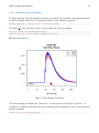
Figure 14 displays the rate (y-axis) at which the read sequence is ”N” (or ”missing”), as a function of
the read position (x-axis). Each line corresponds to one replicate.
This plot can be generated individually with the command:
makePlot.missingness.rate(byLane.plotter);
What it means and what to look for: A number of potential sequencer issues can cause an abrupt ”spike”
or ”shelf” in this plot. In one real sample assessed by QoRTs by the software author, it was determined
that the sequencer camera was slightly offset on one specific cycle of one specific run. All the reads at the
bottom or right edges were lost from that cycle forward, causing the rate of ”N” calls to increase more
than a hundred-fold. Once the problem was recognized the affected reads were identified and removed.
QoRTs Package User Manual
7.4.8
28
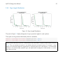
Gene-Body Coverage
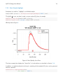
Figure 15: Gene-Body Coverage
For each replicate, the leftmost plot of Figure 15 displays the coverage profile across quantiles of all
genes’ lengths, from 5’ to 3’. The middle plot displays the coverage profile for only the genes that are
in the upper-middle quartile by read-count. The leftmost plot displays the coverage profile for the genes
that are in the two lower quartiles.
Minor notes: To calculate the coverage profile, all the transcripts for each gene are merged together
into a single ”flat” pseudo-transcript which contains all exonic regions belonging to the gene. For each
gene, the pseudo-transcript is broken up into 40 equal-length counting bins, so that each bin contains
2.5% of the total gene length. Each read-pair is counted once for every counting bin with which it
overlaps. Genes are excluded from this analysis if they overlap with other genes or if they have zero reads
for a given replicate. Additionally, any reads that overlap with more than one gene are automatically
excluded.
This plot can be generated individually with the command:
makePlot.genebody.coverage(byLane.plotter);
makePlot.genebody.coverage.UMQuartile(byLane.plotter);
makePlot.genebody.coverage.lowExpress(byLane.plotter);
What it means and what to look for: When run on degraded RNA and/or when using poly-A selection,
RNA-Seq often tends to have ”3’ bias”, in which read coverage is higher on the 3’ end of transcripts. The
degree of this 3’ bias tends to be dependent on the degree of degradation. Many analysis tools are robust
against this issue when it occurs uniformly across the dataset; However, if some samples are substantially
more degraded than others then this may cause problems downstream, particularly if RNA degradation is
associated to the experimental condition(s). When studying this plot, check to make sure the gene-body
coverage is consistant and/or matches your expectations.
Note that the overall gene-body coverage may be strongly influenced by extreme high-coverage genes (and
potentially sequence-specific biases on those specific transcripts). Therefore the upper-middle-quartile plot
is generally the preferred general metric for assessing overall gene-body coverage.
QoRTs Package User Manual
7.4.9
29
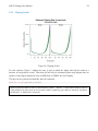
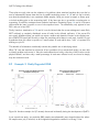
Cumulative Gene Diversity
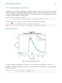
Figure 16: Cumulative Gene Diversity
For each replicate, Figure 16 displays the cumulative gene diversity. For each replicate, the genes are sorted
by read-count. Then, a cumulative function is calculated for the percent of the total proportion of reads as a
function of the number of genes. Intercepts are plotted as well, showing the cumulative percent for 1 gene, 10
genes, 100 genes, 1000 genes, and 10000 genes.
So, for example, across all the replicate, around 50 to 55 percent of the read-pairs were found to map to the
top 1000 genes. Around 20 percent of the reads were found in the top 100 genes. And so on. This can be
used as an indicator of whether a large proportion of the reads stem from of a small number of genes. Note
that this is restricted to only the reads that map to a single unique gene. Reads that map to more than one
gene, or that map to intronic or intergenic areas are ignored.
This plot can be generated individually with the command:
makePlot.gene.cdf(byLane.plotter);
What it means and what to look for: This plot can reveal a number of phenomena. First of all: if the top
few genes dominate a sample (representing a large percentage of the total reads), oddities may appear in
many of the other plots produced by QoRTs, as traits specific to these particular genes are dominant over
the variation found across the genome.
It can also reveal biological variations: Different cell types or cells that are healthy, dying, or under stress
often have very different diversity profiles from one another. If one sample of within a group is an extreme
outlier it may suggest that something is wrong with that sample.
Or technical issues: These plots will often reveal inefficiency of hemoglobin or ribosome depletion protocols, and can also clearly reveal low library complexity (indicated by a very small number of genes being
represented).
QoRTs Package User Manual
7.4.10
30
Nucleotide Rates, by Cycle
Figure 17: Nucleotide rates, by cycle
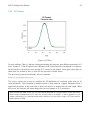
For each replicate, Figure 17 displays the rate at which each nucleotide appears (y-axis), as a function
of the position in the read (x-axis). The color scheme for NVC plots is different from the other plots.
Rather than being used for emphasis or to allow cross-comparisons by sample, biological-condition, or
lane, the colors are used to indicate the four nucleotides: A (green), T (red), G (orange), or C (blue).
Depending on the type of plotter being used, sample-runs will be marked and differentiated by marking
the lines with shapes (R points). In many cases the points will be unreadable due to overplotting, but
clear outliers that stray from the general trends can be readily identified.
When used with a ”sample.highlight” type plotter (see 7.3.5), ”highlighted” samples will be drawn with
a deeper shade of the given color.
This plot displays the ”raw” nucleotide rates, including bases that are soft-clipped by the aligner.
This plot can be generated individually with the command:
makePlot.raw.NVC(byLane.plotter);
What it means and what to look for: This can reveal sequence-specific biases such as hexamer or primer
bias. Additionally, it can reveal adaptor sequencing. Such issues are generally not a problem as long as
they are consistent across samples and groups.
QoRTs Package User Manual
7.4.11
31
Aligned Nucleotide Rates, by Cycle
Figure 18: Aligned nucleotide rates, by cycle
Figure 18 is identical to Figure 17 (described in section 7.4.10), except that it only counts bases that
are not soft clipped off by the aligner.
This plot can be generated individually with the command:
makePlot.minus.clipping.NVC(byLane.plotter);
What it means and what to look for: This can reveal sequence-specific biases such as hexamer or primer
bias. Such issues are generally not a problem as long as they are consistent across samples and groups.
Unlike the raw NVC plot, adaptor sequence will generally be absent from this plot as it usually will not
align to the reference.
QoRTs Package User Manual
7.4.12
32
Leading Clipped Nucleotide Rates
Figure 19: Leading-clipped nucleotide rates
The left plot in Figure 19 displays the nucleotide rate (y-axis) as a function of read position (x-axis), for
the first 6 bases of reads in which exactly 6 bases were clipped off the 5’ end. The right plot displays
the nucleotide rate (y-axis) as a function of read position (x-axis), for the first 12 bases of reads in
which exactly 12 bases were clipped off the 5’ end.
This plot can be generated individually with the command:
makePlot.NVC.lead.clip(byLane.plotter, clip.amt = 6);
makePlot.NVC.lead.clip(byLane.plotter, clip.amt = 12);
Any integer can be used as the clip.amt value.
What it means and what to look for: If a large proportion of the reads are shorter than the read length
then this can reveal the adaptor sequence.
QoRTs Package User Manual
7.4.13
33
Trailing Clipped Nucleotide Rates
Figure 20: Trailing-clipped nucleotide rates
The left plot in Figure 20 displays the nucleotide rate (y-axis) as a function of read position (x-axis), for
the last 6 bases of reads in which exactly 6 bases were clipped off the 3’ end. The right plot displays
the nucleotide rate (y-axis) as a function of read position (x-axis), for the last 12 bases of reads in
which exactly 12 bases were clipped off the 3’ end.
Note concerning the example data: In the example dataset an extremely strong trend is easily visible.
The specific sequence observed matches that of the sequencing adapter used. The pattern appears
in reads coming from fragments that are smaller than the read length. In these cases, the 3’ end of
each read will continue into the adapter sequence after sequencing the entire template fragment. Thus:
for the left and right plots the sequence comes from reads with an insert size of exactly 95 and 89,
respectively (ie 101 base pairs minus 6 or 12).
These plots can be generated individually with the command:
makePlot.NVC.tail.clip(byLane.plotter, clip.amt = 6);
makePlot.NVC.tail.clip(byLane.plotter, clip.amt = 12);
Any integer can be used as the clip.amt value.
What it means and what to look for: If a large proportion of the reads are shorter than the read length
then this can reveal the adaptor sequence.
QoRTs Package User Manual
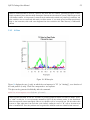
7.4.14
34
Mapping location rates
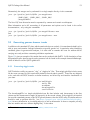
Figure 21: Gene assignment rates
For each replicate, Figure 21 displays the rate (y-axis) for which the replicate’s read-pairs are assigned
to the given categories.
The categories are:
ˆ Unique Gene: The read-pair overlaps with the exonic segments of one and only one gene. For many
downstream analyses tools, such as DESeq, DESeq2 [1] and EdgeR [2], only read-pairs in this category
are used.
ˆ Ambig Gene: The read-pair overlaps with the exons of more than one gene.
ˆ No Gene: The read-pair does not overlap with the exons of any annotated gene.
ˆ No Gene, Intronic: The read-pair does not overlap with the exons of any annotated gene, but appears
in a region that is bridged by an annotated splice junction.
ˆ No Gene, 1kb from gene: The read-pair does not overlap with the exons of any annotated gene, but is
within 1 kilobase from the nearest annotated gene.
ˆ No Gene, 10kb from gene: The read-pair does not overlap with the exons of any annotated gene, but
is within 10 kilobases from the nearest annotated gene.
ˆ No Gene, middle of nowhere: The read-pair does not overlap with the exons of any annotated gene,
and is more than 10 kilobases from the nearest annotated gene.
This plot can be generated individually with the command:
makePlot.gene.assignment.rates(byLane.plotter);
What it means and what to look for: Outliers in these plots can indicate biological variations or the presence
of large mapping problems. They may also suggest the presence of large, highly-expressed, unannotated
transcripts or genes.
QoRTs Package User Manual
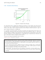
7.4.15
35
Splice Junction Loci
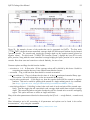
Figure 22: Splice junction loci
For each replicate, Figure 22 displays the number (y-axis) of splice junction loci of each type that appear in
the replicate’s reads. Splice junctions are split into 4 groups, first by whether the splice junction appears in the
transcript annotation gtf (”known” vs ”novel”), and then by whether the splice junction has 4 or more reads
covering it or 1-3 reads.
The six categories of splice junction locus are:
ˆ
ˆ
ˆ
ˆ
ˆ
ˆ
Known: The splice junction locus is found in the supplied transcript annotation gtf file.
Novel: The splice junction locus is NOT found in the supplied transcript annotation gtf file.
Known, 1-3 reads: The locus is known, and is only covered by 1-3 read-pairs.
Known, 4+ reads: The locus is known, and is covered by 4 or more read-pairs.
Novel, 1-3 reads: The locus is novel, and is only covered by 1-3 read-pairs.
Novel, 4+ reads: The locus is novel, and is covered by 4 or more read-pairs.
This plot can be generated individually with the command:
makePlot.splice.junction.loci.counts(byLane.plotter);
What it means and what to look for: This plot can be used to detect a number of anomalies. For example:
whether mapping or sequencing artifacts caused a disproportionate discovery of novel splice junctions in
one sample or batch. It can also be used as an indicator of the comprehensiveness the genome annotation.
Replicates that are obvious outliers may have sequencing/technical issues causing false detection of splice
junctions.
Abnormalities in the splice junction rates are generally a symptom of larger issues which will generally be
picked up by other metrics. Numerous factors can reduce the efficacy by which aligners map across splice
junctions, and as such these plots become very important if the intended downstream analyses include
transcript assembly, transcript deconvolution, differential splicing, or any other form of analysis that in
some way involves the splice junctions themselves. These plots can be used to assess whether other minor
abnormalities observed in the other plots are of sufficient severity to impact splice junction mapping and
thus potentially compromise such analyses.
QoRTs Package User Manual
7.4.16
36
Number of Splice Junction Events
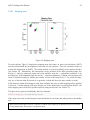
Figure 23: Number of splice junction events
For each replicate, Figure 23 displays the number (y-axis) of all splice junction events falling into each of the
six junction categories. A splice junction ”event” is one instance of a read-pair bridging a splice junction.
Some reads may contain multiple splice junction events, some may contain none. If a splice junction appears
on both reads of a read-pair, this is still only counted as a single ”event”.
Note that because different samples/runs may have different total read counts and/or library sizes, this function
is generally not the best for comparing between samples. In general, the event rates per read-pair should be
used, see the next section, 7.4.17.
This plot is used to detect whether sample-specific or batch effects have a substantial or biased effect on splice
junction appearance, either due to differences in the original RNA, or due to artifacts that alter the rate at
which the aligner maps across splice junctions.
This plot can be generated individually with the command:
makePlot.splice.junction.event.counts(byLane.plotter);
What it means and what to look for: This plot is useful for identifying mapping and/or annotation issues,
and can indicate the comprehensiveness the genome annotation. Replicates that are obvious outliers may
have sequencing/technical issues causing false detection of splice junctions.
In general, abnormalities in the splice junction rates are generally a symptom of larger issues which will
often be picked up by other metrics. See Section 7.4.15.
QoRTs Package User Manual
7.4.17
37
Splice Junction Event Rates per Read-Pair
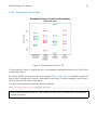
Figure 24: Splice junction events
For each replicate, Figure 24 displays the rate, per read-pair, (y-axis) at which each type of splice
junction events appear. This is equivalent to the results seen in 7.4.16, except that each sample is
scaled by the number of reads belonging to that sample.
This plot can be generated individually with the command:
makePlot.splice.junction.event.ratesPerRead(byLane.plotter);
What it means and what to look for: This plot is used to detect whether sample-specific or batch effects
have a substantial or biased effect on splice junction appearance, either due to differences in the original
RNA, or due to artifacts that alter the rate at which the aligner maps across splice junctions. It can assist
in identifying mapping and/or annotation issues, and can indicate the comprehensiveness the genome annotation. Replicates that are obvious outliers may have sequencing/technical issues causing false detection
of splice junctions.
In general, abnormalities in the splice junction rates are generally a symptom of larger issues which will
often be picked up by other metrics. See Section 7.4.15.
QoRTs Package User Manual
7.4.18
38
Breakdown of Splice Junction Events
Figure 25: Proportions of splice junction events
For each replicate, Figure 25 displays the proportion of all splice junctions events that bridge splice junctions
of each of the six splice junction types.
This plot is used to detect whether sample-specific or batch effects have a substantial or biased effect on splice
junction appearance, either due to differences in the original RNA, or due to artifacts that alter the rate at
which the aligner maps across splice junctions.
This plot can be generated individually with the command:
makePlot.splice.junction.event.proportions(byLane.plotter);
What it means and what to look for: This plot is used to detect whether sample-specific or batch effects
have a substantial or biased effect on splice junction appearance, either due to differences in the original
RNA, or due to artifacts that alter the rate at which the aligner maps across splice junctions. This plot
is useful for identifying mapping and/or annotation issues, and can indicate the comprehensiveness the
genome annotation. Replicates that are obvious outliers may have sequencing/technical issues causing
false detection of splice junctions.
In general, abnormalities in the splice junction rates are generally a symptom of larger issues which will
often be picked up by other metrics. See Section 7.4.15.
QoRTs Package User Manual
7.4.19
39
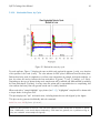
Breakdown of Splice Junction Events, by locus type
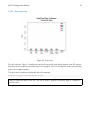
Figure 26: Splice junction events
In Figure 26 the left two columns display the proportion of splice junction events that are known vs
novel. The middle columns display the proportion of known splice junction events that bridge junctions
that have high (more than 4) vs low (1-3) read-pairs covering them. The right two columns display
the proportion of novel splice junction events that bridge junctions that have high (more than 4) vs low
(1-3) read-pairs covering them.
This plot can be generated individually with the command:
makePlot.splice.junction.event.proportionsByType(byLane.plotter);
What it means and what to look for: This plot is useful for identifying mapping and/or annotation issues,
and can indicate the comprehensiveness the genome annotation. Replicates that are obvious outliers may
have sequencing/technical issues causing false detection of splice junctions.
In general, abnormalities in the splice junction rates are generally a symptom of larger issues which will
often be picked up by other metrics. See Section 7.4.15.
QoRTs Package User Manual
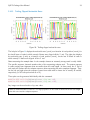
7.4.20
40
Strandedness test
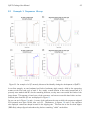
Figure 27: Strandedness
Figure 27 displays the rate at which reads appear to follow the two possible library-type strandedness
rules. (See section 6 for more information on stranded library types).
This plot is used to detect whether your data is indeed stranded, and whether you are using the correct
stranded data library type option. For unstranded libraries, one would expect all points to fall very close
to the 50-50 center line. For stranded libraries, all points should fall closer to 99
This plot can be generated individually with the command:
makePlot.strandedness.test(byLane.plotter);
What it means and what to look for: This plot can indicate the efficiency of the strand-specific selection
protocol, and reveal variations in such efficiency. They can also be used to determine the ”strandedness
rule”, which is required by many downstream analysis tools.
QoRTs Package User Manual
7.4.21
41
Mapping stats
Figure 28: Mapping stats
For each replicate, Figure 28 displays the mapping rates and counts. In order to plot this data, QoRTs
must be provided with the pre-alignment read-count for each replicate. There are a number of ways to
provide this information to QoRTs. The easiest method is to list it specifically in the replicate decoder
(see Section ??). Alternatively, this information can be provided at the initial processing stage (see
Section 6), either by setting the input read count explicitly using the --seqReadCt parameter, or by
providing one of the unaligned fastq files via the --rawfastq parameter, in which case the input read
count is calculated simply by dividing the number of lines in the fastq file by 4. For paired-end data,
only one of the two fastq files needs to be provided, as both will have the same number of reads.
If the dataset contains multi-mapped reads, then numbers and rates of multi-mapping will be included
in this plot. If multi-mapped reads were filtered out of the dataset prior to analysis with QoRTs, the
multi-mapping rates can still be specified explicitly using the decoder (see Section ??).
This plot can be generated individually with the command:
makePlot.mapping.rates(byLane.plotter);
If the input read count or multi-mapped count information is not found, this will generate a placeholder
plot.
What it means and what to look for: Presence of outliers in the mapping rate statistics may be an indicator
of large sample-prep, library-prep, or sequencer errors.
QoRTs Package User Manual
7.4.22
42
Chromosome counts
Figure 29: Mapping stats
For each replicate, Figure 29 displays the number of read-pairs mapping to each category of chromosome.
The chromosome.name.style must be set to match the style of your chromosome names. By default
it assumes the chromosomes are named chr1, chr2, chr3, etc.
For more information, see the help document using the command help(makePlot.chrom.type.rates).
This plot can be generated individually with the command:
makePlot.chrom.type.rates(byLane.plotter);
What it means and what to look for: Presence of outliers in these plots may point to variable inefficiency
in a ribosomal/mitochondrial depletion protocol. In most datasets the Y chromosome counts can be used
to determine sample sex (but not in this case, since the Y chromosome is not included in the example
dataset’s genome assembly). The raw metrics generated by QoRTs can also be used to generate counts
for the ERCC spike-ins or similar.
QoRTs Package User Manual
7.4.23
43
Normalization Factors
Figure 30: Normalization Factors
For each replicate, Figure 30 displays the normalization factors.
By default, QoRTs will automatically detect whether DESeq2 and edgeR are installed and will use
these tools to calculate their respective normalization size factors. If neither package is found, then it
will only plot the total count normalization.
This plot can be generated individually with the command:
makePlot.norm.factors(byLane.plotter);
What it means and what to look for: These normalization factors can be used for a number of downstream
analyses, including the generation of summary browser tracks.
QoRTs Package User Manual
7.4.24
44
Normalization Factor Ratio
Figure 31: Normalization Factors vs TC
For each replicate, Figure 31 displays the ratio of the alternate normalization factors to the Total Count
normalization factors.
By default, QoRTs will automatically detect whether DESeq2 and edgeR are installed and will use
these tools to calculate their respective normalization size factors. If neither package is found, then it
will only plot the total count normalization.
This plot can be generated individually with the command:
makePlot.norm.factors.vs.TC(byLane.plotter);
What it means and what to look for: Large variations in these ratios can indicate large-scale differences
between the samples.
QoRTs Package User Manual
7.4.25
45
Read drop rate
Figure 32: Drop rates
For each replicate, Figure 32 displays the rates and reasons for reads being dropped from QC analysis.
Note that in the example dataset reads were never dropped. This is a consequence of the pre-processing
steps in the example pipeline.
This plot can be generated individually with the command:
makePlot.dropped.rates(byLane.plotter);
What it means and what to look for: This can be used to assess the occurrance rates of a number of
failure modes.
QoRTs Package User Manual
8
46
Identifying Problems
QoRTs produces a vast array of output data, and the interpretation of said data can be difficult.
Proper quality control must consider the study design, sequencer technology, study species, read length,
library preparation protocol, and numerous other factors that might affect the metrics produced by
QoRTs. In some datasets, apparent ”abnormalities” may be expected. Similarly, depending on the type
of downstream analysis that is being performed, some errors or artifacts may be irrelevant.
When an unexplained abnormality is recognized, one must decide what to do with the data. Unfortunetely this question is nontrivial, and depends on numerous factors. Bioinformaticians must be aware
of the statistical assumptions that are being made in the downstream analyses, and must consider the
conditions under which such assumptions would be violated.
Some abnormalities will not affect a given analysis and thus can be ignored outright. Some may require
that the offending sample(s) be removed from the analysis. Others may necessitate additional steps to
normalize the data or adjust for confounding factors. And finally, some artifacts may be so severe that
the intended analysis will be impossible using the supplied data. Ultimately bioinformaticians must use
their own judgement to determine what action should be taken, should an abnormality be discovered.
Here we present two examples of data-quality issues that were incidentally discovered during the development of the QoRTs software package. Note that the sequencing data presented in these examples
are atypical, and were chosen because they illustrated succinctly the abnormalities in the data.
QoRTs Package User Manual
8.1
47
Example 1: Sequencer Hiccup
Figure 33: An example of a QC anomaly discovered incidentally during the development of QoRTs.
In our first example, an rare hardware-level fault of unknown origin caused a shift in the sequencing
scanner at the 53rd read cycle of read 2. As a result, a small fraction of the reads (around half of a
percent) were marked with N’s for the remaining 48 bases, as they were now outside the limits of the
image frame. This appears to have been a freak occurance: we have not seen this issue before or since.
Selected plots from this QC run are displayed in Figure 33.
As you can see in Figure 33a and c, in some of the replicates the rate at which the sequencer assigned
N’s increased more than 10-fold after cycle 53. Furthermore, in figures 33b and d, the replicates
also displayed a small but abrupt increase in the clipping rate. This was due to the fact that aligner
(RNA-Star) always clipped reads when they had no remaining ”called” nucleotides.
QoRTs Package User Manual
48
These plots not only point out the existance of a problem, when examined together they can also be
used to substantially narrow down the list of possibile underlying causes. In 33a and b it can be clearly
seen that the abnormality is not consistent within samples, ruling out errors in sample or library prep,
or indeed anything prior to the sequencing itself. If the issue was due to an artifact occurring prior to
sequencing, it would be consistent across technical replicates. Examining Figure 33c and d, it becomes
obvious that the issue is specific to one of the sequencer lanes. The abnormality only appears in lane
RG2, and not in lane RG1.
Finally, based on examination of 33b and d it can be inferred that the excess missingness is most likely
NOT uniformly or randomly distributed across all reads in the affected replicates. If the excess N’s
were evenly distributed then you would not expect a sudden and dramatic increase in the clipping rate,
since RNA-STAR would still be able to align the remaining called bases in each read. Instead, we can
hypothesize that this effect is specific to a small subset of reads which have ”tails” of repeated N’s
starting at cycle 53.
This breadth of information considerably narrows the possible set of underlying causes.
When ”N” rate was examined as a function of lane coordinate (via a custom-built script), we were able
to identify problem and correct it. Since the reads affected were solely a function of the location on the
physical flowcell, and since only a small percentage of reads were affected at all, we elected to simply
drop the truncated reads.
8.2
Example 2: Badly Degraded RNA
Figure 34: Another example of a QC anomaly discovered incidentally during the development of QoRTs.
In our second case study, one particular RNA sample was substantially more degraded than the others.
All samples were poly-A selected, so this heightened degradation resulted in a strong 3’ bias.
QoRTs Package User Manual
49
In Figure 34 the affected sample is plotted in red and blue (indicating the two technical replicates),
whereas all the other samples are plotted in grey. The vastly-increased 3’ bias can be clearly identified in
34a. Figure 34b shows that this had a substantial effect on the rate at which splice junction events were
observed. Excess 3’ bias can have broad impact, compromising estimates of gene-level and transcriptlevel abundance, and consequently compromising differential expression or differential splicing analyses.
As a result, outliers like this should generally be dropped prior to analysis.
QoRTs Package User Manual
9
50
Secondary Utilities
In addition to the standard quality-control tools described in the previous sections, QoRTs also includes
a number of other minor utilities intended to assist in data visualization, cleaning, and preparation for
downstream analyses.
9.1
Generating a flattened annotation file
Before counting exons and splice junctions, QoRTs generates a set of non-overlapping exonic fragments
out of all the exons in the genome annotation gtf file. It then assigns each exonic fragment a unique
identifier. Similarly, it assigns every splice junction its own unique identifier. A gtf file listing all these
genomic features and their unique identifiers can be created using the following command:
java -jar /path/to/jarfile/QoRTs.jar makeFlatGtf \
input.gtf \
flattened.gff
Both the input and output annotation files can be either .zip or .gz compressed. Compression is
autodetected from the file extension.
strandedness: You must use the --stranded option to create the flattened gff for use with stranded
datasets. DO NOT mix stranded flattened gff with unstranded data, or vice versa.
DEXSeq: DEXSeq also requires a flattened annotation file, which is formatted similarly. In order to
produce a flattened gff file that DEXSeq can read, include the --DEXSeqFmt option.
This gtf file conforms to the UCSC gff file definition, (found here: http://genome.ucsc.edu/FAQ/
FAQformat.html). It will contain 4 different feature types (column 3): ”aggregate gene”, ”exonic part”, ”splice site”, and ”novel splice site”.
9.2
Merging Count Data
For the purposes of quality control it is generally preferable to run QoRTs on each sample-run individually, so that potential technical artifacts related to sequencing run or lane can be identified. However,
for most downstream purposes these ”technical replicates” will be combined and treated as a single
sample. Differential expression tools like DESeq, DESeq2 [1], DEXSeq [3], and EdgeR [7] assume that
each set of gene counts (or exon counts, for DEXSeq) is derived from a different biological sample.
Thus, the java utility includes a function for quickly and easily calculating merged sample-wise counts:
java -jar /path/to/jarfile/QoRTs.jar mergeAllCounts \
decoder.txt \
/path/to/qc/results/dir/
./merged/
This decoder MUST contain the unique.ID and sample.ID columns.
\
QoRTs Package User Manual
51
Alternatively, the merger can be performed for a single sample directly, via the command:
java -jar /path/to/jarfile/QoRTs.jar mergeCounts
./SAMP1_RG1/,./SAMP1_RG2/,./SAMP1_RG3/
./merged/SAMP1/
The list of QC data directories must be separated by commas and contain no whitespace.
More information and a full accounting of all parameters and options can be found in the online
documentation7 , or by using the commands:
java -jar /path/to/jarfile/QoRTs.jar mergeAllCounts--man
and
java -jar /path/to/jarfile/QoRTs.jar mergeCounts --man
9.3
Generating genome browser tracks
In addition to the standard QC plots, which examine the data as a whole, it is sometimes desirable to be
able to query and examine coverage information at specific genetic loci. In particular, when identifying
candidate genes via genome-wide analyses, it is often vital to examine the locus for artifacts before
carrying out costly and time-consuming validation experiments.
Figure 35 is just one example of the tracks that can be produced with QoRTs. A full description of how
this particular splice junction track can be generated can be found in the example dataset walkthrough,
which is linked to on the QoRTs github site.
9.3.1
Generating wiggle tracks
QoRTs includes a utility to generate ”.wig”, or ”wiggle plot” files. These wiggle plot files include counts
for the mean coverage for each equal-sized window across the whole genome. These files are designed
to be used with the UCSC browser or similar interfaces, and allow easy and intuitive visualization of
your data.
java -jar /path/to/jarfile/QoRTs.jar bamToWiggle
infile.bam
trackName
chromLengthFile
outfilePrefix
The chromLengthFile is a simple tab-delimited text file that includes each chromosome in the first
column and the chromosome’s length (in base-pairs) in the second column. If the wiggle file is intended
for use with a standard genome on the UCSC genome browser, then the UCSC utility fetchChromSizes
should be used to generate this file. (see http://genome.ucsc.edu/goldenPath/help/bigWig.
html for more information on fetchChromSizes, as well as information on how to compress your wig
files into smaller and more efficient bigWig files). It also takes
7
Found here: http://hartleys.github.io/QoRTs/jarHtml/index.html
QoRTs Package User Manual
52
Figure 35: An example of some of the tracks that can be generated via QoRTs. The first track
(”CTRL FWD”) shows the mean normalized coverage depth for 100-base-pair windows for the forward
(genomic) strand. The second track reveals the coverage depth on the negative strand (plotted as
negative values). The third track (”CASEvCTRL Junction Counts”) displays the locus ID for each
splice junction, along with the mean normalized coverage bridging the splice junction loci in cases and
controls. Note that cases and controls are colored distinctly, for ease of use.
Common options and flags for this function include:
--sizefactor 1.0 : A float value. All the coverage values will be divided by this factor. Useful for
comparing two samples that may have different normalization factors.
--stranded : Flag to indicate that data should be treated as stranded.
--fr secondStrand : Flag to indicate that the data is of the fr secondstrand stranded library type.
(See section 6 for more information on the two stranded library types).
--negativeReverseStrand : If this flag is set, then the negative strand will be counted in negative
numbers. This can be useful for plotting both strands in a single multiwig track, via a trackhub.
(see http://genome.ucsc.edu/goldenPath/help/trackDb/trackDbDoc.html)
--simpleCountByRead : If this flag is raised, then each read of each read-pair will be counted separately. Thus the wiggle plot will count simple read coverage depth rather than read-pair coverage
depth. This means that when read-pairs overlap they will be counted twice over the overlapping
region. This option will have no effect on single-ended data.
Many of the other parameters are identical to those used by the QC tool: --singleEnded, --nameSorted,
etc.
More information and a full accounting of all parameters and options can be found in the online
documentation8 , or by using the command:
8
Found here: http://hartleys.github.io/QoRTs/jarHtml/index.html
QoRTs Package User Manual
53
java -jar /path/to/jarfile/QoRTs.jar bamToWiggle --man
9.3.2
Merging wiggle tracks
QoRTs includes a utility for summing or averaging multiple wiggle files, either with or without normalization factors. For example, to calculate the normalized mean coverage for each 100-bp window across
all CASE samples in the example dataset:
java -jar /path/to/jarfile/QoRTs.jar mergeWig \
--calcMean \
--filenames outputData/countTables/SAMP1/QC.wiggle.fwd.wig.gz,output\
Data/countTables/SAMP2/QC.wiggle.fwd.wig.gz,outputData/countTables/SAMP3/QC.wiggle.f\
wd.wig.gz \
--sizeFactors 1.057995,0.999932,1.015372 \
path/to/output/CASE.fwd.wig.gz
There are a number of other alternative parameterizations. The --sampleList parameter (which
can be either a comma-delimited list or a ”.txt” file containing a list) can be used along with the
--infilePrefix and --infileSuffix to specify the file names if all of the wiggle files are in
the same parent directory. The size factors can also be provided in a tab-delimited file using the
--sizeFactorFile parameter. If the --sizeFactors and --sizeFactorFile parameters are omitted then the non-normalized sums/means will be calculated.
Common options and flags for this function include:
--calcMean : If this flag is raised, the utility will calculate the average rather than the total coverage
for each window.
--makeNegative : If this flag is raised, all output values will be multiplied by -1.
--sizeFactorFile : A file containing at least two columns, the sample.ID and the size.factor. This
file must include all samples in the sample list, but can include other samples that are not included
in the sample list.
More information and a full accounting of all parameters and options can be found in the online
documentation9 , or by using the command:
java -jar /path/to/jarfile/QoRTs.jar mergeWig --man
9.3.3
Generating splice-junction tracks
To visualize splice junction data, QoRTs can produce bed files that show splice junction counts:
java -jar /path/to/jarfile/QoRTs.jar makeJunctionTrack \
--stranded \
--filenames outputData/countTables/SAMP1/QC.spliceJunctionAndExonCou\
nts.withNovel.forJunctionSeq.txt.gz \
9
Found here: http://hartleys.github.io/QoRTs/jarHtml/mergeWig.html
QoRTs Package User Manual
54
flattened.gff \
path/to/output/CASE.bed.gz
Common options and flags for this function include:
--rgb r,g,b : The color to use for each bed entry. Three integers, comma-delimited (with no spaces),
each between 0 and 255.
--stranded : Whether the data is stranded.
--sizeFactors sf1,sf2,... : A list of size factors with which to normalize replicates to a common
scale. The list must have the same length as the number of replicates provided (ie the filenames
parameter).
--skipNovelJunctions : If this option is used, novel splice junctions will not be included in the
output file.
--title : A prefix to append to each splice junction ID.
More information and a full accounting of all parameters and options can be found in the online
documentation10 , or by using the command:
java -jar /path/to/jarfile/QoRTs.jar makeJunctionTrack --man
9.3.4
Merging splice-junction tracks
Merged splice junction tracks can be created using the same utility used to create single-sample splice
junction tracks. This uses syntax similar to the syntax used for merging wiggle files:
java -jar /path/to/jarfile/QoRTs.jar makeJunctionTrack \
--calcMean \
--stranded \
--filenames outputData/countTables/SAMP1/QC.spliceJunctionAndExonCo\
unts.withNovel.forJunctionSeq.txt.gz,outputData/countTables/SAMP2/QC.spliceJunctionA\
ndExonCounts.withNovel.forJunctionSeq.txt.gz,outputData/countTables/SAMP3/QC.spliceJ\
unctionAndExonCounts.withNovel.forJunctionSeq.txt.gz \
--sizeFactors 1.057995,0.999932,1.015372 \
flattened.gff \
path/to/output/CASE.bed.gz
As with the wiggle-file merge utility, there are a number of other alternative parameterizations. The
--sampleList parameter (which can be either a comma-delimited list or a ”.txt” file containing a list)
can be used along with the --infilePrefix and --infileSuffix to specify the file names if all of the
wiggle files are in the same parent directory. The size factors can also be provided in a tab-delimited file
using the --sizeFactorFile parameter. If the --sizeFactors and --sizeFactorFile parameters
are omitted then the non-normalized sums/means will be calculated.
More information and a full accounting of all parameters and options can be found in the online
documentation11 , or by using the command:
10
11
Found here: http://hartleys.github.io/QoRTs/jarHtml/makeJunctionTrack.html
Found here: http://hartleys.github.io/QoRTs/jarHtml/makeJunctionTrack.html
QoRTs Package User Manual
55
java -jar /path/to/jarfile/QoRTs.jar makeJunctionTrack --man
9.4
Importing data into other tools
In addition to providing quality control information, QoRTs also provides the requisite input files needed
for the DESeq/DESeq2 [1], DEXSeq [3], and EdgeR [2, 7, 8] analysis tools. These files will be identical
to those that would be generated by HTSeq (using the default ”union rule” option).
All the data files can be found in the qc.data.dir directory. The files for use with DESeq, DESeq2 ,
and EdgeR will be named QC.geneCounts.formatted.for.DESeq.txt.gz and the files for use with
DEXSeq will be named QC.exonCounts.formatted.for.DEXSeq.txt.gz
9.4.1
DEXSeq compatibility
A note on the DEXSeq counts: The DEXSeq counts may not be perfectly identical to those produced by
the dexseq_prepare_annotation.py and dexseq_count.py scripts. There are two reasons for these
differences, both relating to the treatment of aggregate genes. The first reason is minor: Aggregate
genes will be named slightly differently. When multiple genes overlap with one another, DEXSeq
produces ”aggregate genes” which include all transcripts for all these overlapping genes. It names the
aggregate gene using the set of genes in the aggregate, delimited with + characters. Unfortunately, the
genes are drawn from an unordered set and thus not listed in any defined order. Thus, it is not possible
for QoRTs to replicate the exact same order in multi-gene aggregates. QoRTs lists the contained genes
in lexicographic order.
Secondly, for UNSTRANDED data, the QoRTs and DEXSeq annotation ”flattening” step will behave
slightly differently under default conditions. DEXSeq’s dexseq_prepare_annotation.py script always operates in ”stranded” mode, and explicitly destinguishes between genes on opposing strands.
QoRTs, on the other hand, prepares the flattened annotation in stranded or unstranded modes. If the
DEXSeq-style behavior is desired, a stranded flat gff file can be produced by the makeFlatGff utility,
then passed explicitly to the QoRTs QC utility running in non-stranded mode using the --flatgff
parameter. This will override the default (and recommended) behavior in which the flattened gff will
use the same stranded rule as the counting utility. Warning: if this variation is used, the counting run
should be restricted to only the DEXSeq-count utility using the additional parameter: ”–runFunctions
writeDEXSeq”. The behavior of the other QoRTs utilities when run with a nonmatching flattened
annotation is not defined.
In general, testing aggregate genes in DEXSeq is not recommended, as the two genes are likely to be
independently regulated and will likely produce false positives. For most purposes it is preferable to
drop such genes from the count tables prior to DEXSeq analysis. In this case, the counts produced by
DEXSeq and QoRTs will be identical.
QoRTs Package User Manual
56
References
[1] Simon Anders and Wolfgang Huber. Differential expression analysis for sequence count data.
Genome Biology, 11:R106, 2010. URL: http://genomebiology.com/2010/11/10/R106.
[2] Mark D. Robinson and Gordon K. Smyth.
Moderated statistical tests for assessing differences in tag abundance.
Bioinformatics, 23:2881, 2007.
URL:
http://bioinformatics.oxfordjournals.org/cgi/content/abstract/23/21/2881,
http://arxiv.org/abs/http://bioinformatics.oxfordjournals.org/cgi/reprint/23/21/2881.pdf
arXiv:http://bioinformatics.oxfordjournals.org/cgi/reprint/23/21/2881.pdf,
doi:10.1093/bioinformatics/btm453.
[3] Simon Anders, Alejandro Reyes, and Wolfgang Huber. Detecting differential usage of exons from
RNA-seq data. Genome Research, 22:2008, 2012. doi:10.1101/gr.133744.111.
[4] Alexander Dobin, Carrie A. Davis, Felix Schlesinger, Jorg Drenkow, Chris Zaleski, Sonali Jha, Philippe Batut, Mark Chaisson, and Thomas R. Gingeras.
STAR: ultrafast universal RNA-seq aligner.
Bioinformatics, 29(1):15–21, 2013.
URL:
http://bioinformatics.oxfordjournals.org/content/29/1/15.abstract,
http://arxiv.org/abs/http://bioinformatics.oxfordjournals.org/content/29/1/15.full.pdf+html
arXiv:http://bioinformatics.oxfordjournals.org/content/29/1/15.full.pdf+html,
doi:10.1093/bioinformatics/bts635.
[5] Thomas D. Wu and Serban Nacu.
Fast and SNP-tolerant detection of complex variants and splicing in short reads.
Bioinformatics, 26(7):873–881, 2010.
http://bioinformatics.oxfordjournals.org/content/26/7/873.abstract,
URL:
http://arxiv.org/abs/http://bioinformatics.oxfordjournals.org/content/26/7/873.full.pdf+html
arXiv:http://bioinformatics.oxfordjournals.org/content/26/7/873.full.pdf+html,
doi:10.1093/bioinformatics/btq057.
[6] Daehwan Kim, Geo Pertea, Cole Trapnell, Harold Pimentel, Ryan Kelley, and Steven Salzberg.
Tophat2: accurate alignment of transcriptomes in the presence of insertions, deletions and gene
fusions. Genome Biology, 14(4):R36, 2013. URL: http://genomebiology.com/2013/14/4/R36,
http://dx.doi.org/10.1186/gb-2013-14-4-r36 doi:10.1186/gb-2013-14-4-r36.
[7] McCarthy DJ Robinson MD and Smyth GK. edger: a bioconductor package for differential expression
analysis of digital gene expression data. Bioinformatics, 26:139–140, 2010.
[8] Davis J. McCarthy, Yunshun Chen, and Gordon K. Smyth. Differential expression analysis of multifactor RNA-Seq experiments with respect to biological variation. Nucleic Acids Research, 40:4288–
4297, 2012.
10
Session Information
The session information records the versions of all the packages used in the generation of the present
document.
QoRTs Package User Manual
57
sessionInfo()
##
##
##
##
##
##
##
##
##
##
##
##
##
##
##
##
##
##
##
##
##
##
##
##
##
##
##
##
##
##
##
##
##
##
##
R version 3.1.1 (2014-07-10)
Platform: x86_64-unknown-linux-gnu (64-bit)
locale:
[1] C
attached base packages:
[1] parallel stats4
stats
[8] methods
base
other attached packages:
[1] edgeR_3.8.2
[4] RcppArmadillo_0.4.500.0
[7] GenomeInfoDb_1.2.2
[10] BiocGenerics_0.12.0
[13] Cairo_1.5-6
graphics
grDevices utils
limma_3.22.1
Rcpp_0.11.3
IRanges_2.0.0
QoRTsExampleData_0.2.0
knitr_1.7
loaded via a namespace (and not attached):
[1] AnnotationDbi_1.28.1 BBmisc_1.8
[4] Biobase_2.26.0
BiocParallel_1.0.0
[7] DBI_0.3.1
Formula_1.1-2
[10] MASS_7.3-35
RColorBrewer_1.0-5
[13] XML_3.98-1.1
XVector_0.6.0
[16] annotate_1.44.0
base64enc_0.1-2
[19] checkmate_1.5.0
cluster_1.15.3
[22] colorspace_1.2-4
digest_0.6.4
[25] fail_1.2
foreach_1.4.2
[28] formatR_1.0
genefilter_1.48.1
[31] ggplot2_1.0.0
grid_3.1.1
[34] highr_0.4
iterators_1.0.7
[37] latticeExtra_0.6-26 locfit_1.5-9.1
[40] nnet_7.3-8
plyr_1.8.1
[43] reshape2_1.4
rpart_4.1-8
[46] sendmailR_1.2-1
splines_3.1.1
[49] survival_2.37-7
tools_3.1.1
11
datasets
DESeq2_1.6.1
GenomicRanges_1.18.1
S4Vectors_0.4.0
QoRTs_0.3.4
BatchJobs_1.5
BiocStyle_1.4.1
Hmisc_3.14-5
RSQLite_1.0.0
acepack_1.3-3.3
brew_1.0-6
codetools_0.2-9
evaluate_0.5.5
foreign_0.8-61
geneplotter_1.44.0
gtable_0.1.2
lattice_0.20-29
munsell_0.4.2
proto_0.3-10
scales_0.2.4
stringr_0.6.2
xtable_1.7-4
Legal
This software is ”United States Government Work” under the terms of the United States Copyright
Act. It was written as part of the authors’ official duties for the United States Government and thus
cannot be copyrighted. This software is freely available to the public for use without a copyright notice.
QoRTs Package User Manual
58
Restrictions cannot be placed on its present or future use.
Although all reasonable efforts have been taken to ensure the accuracy and reliability of the software
and data, the National Human Genome Research Institute (NHGRI) and the U.S. Government does not
and cannot warrant the performance or results that may be obtained by using this software or data.
NHGRI and the U.S. Government disclaims all warranties as to performance, merchantability or fitness
for any particular purpose.
In any work or product derived from this material, proper attribution of the authors as the source of
the software or data should be made, using ”NHGRI Genome Technology Branch” as the citation.
The QoRTs Scala package includes (internally) the sam-JDK library (sam-1.113.jar) from picard tools,
which is licensed under the MIT license: The MIT License Copyright (c) 2009 The Broad Institute
Permission is hereby granted, free of charge, to any person obtaining a copy of this software and
associated documentation files (the ”Software”), to deal in the Software without restriction, including
without limitation the rights to use, copy, modify, merge, publish, distribute, sublicense, and/or sell
copies of the Software, and to permit persons to whom the Software is furnished to do so, subject
to the following conditions: The above copyright notice and this permission notice shall be included
in all copies or substantial portions of the Software. THE SOFTWARE IS PROVIDED ”AS IS”,
WITHOUT WARRANTY OF ANY KIND, EXPRESS OR IMPLIED, INCLUDING BUT NOT LIMITED
TO THE WARRANTIES OF MERCHANTABILITY, FITNESS FOR A PARTICULAR PURPOSE AND
NONINFRINGEMENT. IN NO EVENT SHALL THE AUTHORS OR COPYRIGHT HOLDERS BE
LIABLE FOR ANY CLAIM, DAMAGES OR OTHER LIABILITY, WHETHER IN AN ACTION OF
CONTRACT, TORT OR OTHERWISE, ARISING FROM, OUT OF OR IN CONNECTION WITH
THE SOFTWARE OR THE USE OR OTHER DEALINGS IN THE SOFTWARE.
The MIT license and copyright information can also be accessed using the command:
java -jar /path/to/jarfile/QoRTs.jar "?" samjdkinfo