1
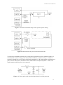
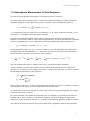
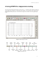
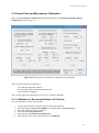
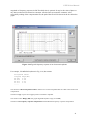
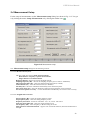
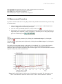
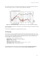
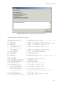
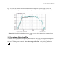
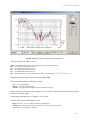
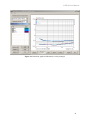
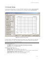
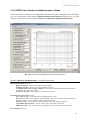
STEPS Program for Frequency Response Measurements Using Heterodyned Stepped Sine Technique User Manual Version 1.8.5 Ivo Mateljan Artalabs J. Rodina 4, 21215 Kaštel Lukšić, Croatia February, 2015. Copyright © Ivo Mateljan, 2004 - 2015. All rights reserved. STEPS User Manual Content 1 INTRODUCTION .............................................................................................................................................. 3 1.1 REQUIREMENTS ............................................................................................................................................. 3 1.2 MEASUREMENT HARDWARE SETUP ............................................................................................................... 3 1.3 HETERODYNED MEASUREMENT OF SINE RESPONSE ...................................................................................... 5 2 USING STEPS FOR STEPPED-SINE TESTING .......................................................................................... 8 2.1 STEPS MENUS ............................................................................................................................................ 11 2.2 AUDIO DEVICES SETUP ................................................................................................................................ 13 2.2.1 WDM Audio Driver Setup for Windows 2000 / XP ............................................................................. 14 2.2.2 WDM Audio Driver Setup for Windows Vista / 7 / 8 ........................................................................... 16 2.2.3 ASIO driver setup ................................................................................................................................ 18 2.3 SOUND CARD AND MICROPHONE CALIBRATION .......................................................................................... 19 2.3.1 Calibration of Soundcard Output Left Channel .................................................................................. 19 2.3.2 Calibration of Soundcard Input Channels ........................................................................................... 20 2.3.3 Calibration of the Microphone ............................................................................................................ 20 2.3.4 Frequency Response Compensation .................................................................................................... 20 2.4 MEASUREMENT SETUP ................................................................................................................................ 22 2.5 MEASUREMENT PROCEDURE ....................................................................................................................... 23 2.6 OVERLAYS ................................................................................................................................................... 24 2.7 FILE MANIPULATIONS.................................................................................................................................. 25 2.8 GRAPH SETUP AND EDITING ........................................................................................................................ 28 2.8.1 GRAPH SETUP ........................................................................................................................................... 28 2.8.2 Editing graph colors and line style ...................................................................................................... 29 2.8.3 Editing plotted curve ........................................................................................................................... 31 2.8.4 Low Frequency Loudspeaker Box Diffraction Scaling ........................................................................ 32 2.9 PERCENTAGE DISTORTION PLOT.................................................................................................................. 33 2.10 TIME RECORD ............................................................................................................................................ 36 3. USING STEPS FOR STEPPED-AMPLITUDE TESTING ........................................................................ 38 3.1 DISTORTION VS. AMPLITUDE TESTING......................................................................................................... 38 3.2 LINEARITY TESTING .................................................................................................................................... 42 3.3. DISPLACEMENT AND DISTORTIONS TESTING ............................................................................................. 44 3.3.1 Definition of Xmax............................................................................................................................... 44 3.3.2 Measurement of Xmax ......................................................................................................................... 44 3.3.3 STEPS user interface for measurement of Xmax ................................................................................. 46 3.4 LOUDSPEAKER DISTORTION LIMITED MAXIMUM SPL .................................................................................. 48 2 STEPS User Manual 1 Introduction The STEPS is a program for frequency response measurement using a heterodyned stepped-sine technique. Compared to the Fourier analyzer, that uses a random noise excitation, this technique gives a larger dynamic range (at least 30dB), but measurements are much slower. This program is also useful for measuring harmonic distortions as it estimates the linear part of the system response and the magnitude of distorted sine harmonics. 1.1 Requirements Minimum requirements to use the STEPS are: o o o o Operating systems: Windows XP / Vista / 7 / 8 Processor class Pentium, clock frequency 600 MHz or higher, memory 256M for Windows 2000/XP or 2MB for Vista/Windows 7 Full duplex soundcard with synchronous clock for AD and DA converters WDM or ASIO soundcard driver (ASIO is trademark and software of Steinberg Media Technologies GmbH). The Installation of this software is easy; use ARTA installation program or just copy the program "steps.exe" and the help file "steps.chm" in some folder and make a shortcut to it. All registry data will be automatically saved at the first program execution. Files with extension ".HSW" are registered to be opened with the program STEPS. They contain the frequency response data. Results of measurements can also be saved as textual - ASCII formatted files. The STEPS does not output graphs to the printer, instead all graphs can be copied to the Windows Clipboard and pasted to other Windows applications. 1.2 Measurement Hardware Setup In this document, we refer to following measurement setups: 1. Dual channel measurement setup 2. Single channel measurement setup The general measurement setup for the system testing is shown in Fig. 1.1. The soundcard left lineoutput channel is used as a signal generator output. The left line-input is used to measure a D.U.T. output voltage and the right line-input is used to measure a D.U.T. input voltage. In a single channel setup, only a D.U.T. output voltage is recorded. The setup for acoustical measurements is shown in Fig. 1.2. 3 STEPS User Manual Figure 1.1 General measurement setup for the system response testing Figure 1.2 Measurement setup for acoustical measurements To protect the soundcard input form large voltage that is generated at a power amplifier output, it is recommended to use the voltage probe circuit with Zener diodes, as shown on Fig. 1.3. Values of resistors R1 and R2 have to be chosen for arbitrary attenuation (i.e. R1=8200 and R2=910 ohms gives probe with -20.7dB (0.0923) attenuation if the soundcard has usual input impedance - 10kΩ). In a single channel mode this probe is not connected. Figure 1.3 Voltage probe with soundcard input channel overload protection 4 STEPS User Manual 1.3 Heterodyned Measurement of Sine Response The idea of a heterodyned measurement of a sinusoidal response is as follows. We assume that a time-invariant system is excited with a sinusoidal signal g(t) of known frequency, amplitude and phase. At the output of the system we measure a noisy and distorted signal y(t); y (t ) A1 sin(t 1 ) N A sin( kt k k) n(t ) k 2 A1 is a amplitude of the base sinusoid (or base harmonic), 1 is a phase of the base sinusoid, n(t) is a noise and Ak is a amplitude of k-th harmonic (distortion). We want to estimate the amplitude and the phase of harmonic components with a minimal noise influence. We can achieve that by using a heterodyned technique; we extract k-th harmonic component from y(t) by multiplying it with a complex form of the input signal that has known frequency ; gk (t ) sin( kt ) j cos(kt ) je jkt , i 1,2,... and integrating the product y(t) gk(t) in a time T. What we get is k-th signal harmonic filtered with a heterodyne filter of bandwidth equal to 1/T. The former procedure is equivalent to the estimation of the k-th harmonic component by the Fourier series expansion: T ck j T 1 A A 1 y (t )e j kt dt k cos k j k sin k j (other _ harmonics noise )e j kt dt T 0 2 2 T 0 Note: the multiplication with j is arbitrary; that way we get the proper phase estimation. An exact solution is possible only if there is no noise and if the integration time T is equal to the multiple of 1/. In that case, the integral term of other_harmonics is equal to the zero and we estimate the amplitude and the phase by the expression: Ak 2 Re( ck ) 2 Im( ck ) 2 k arctan( Im( ck ) ) Re( ck ) In the presence of the noise, we have a biased estimation, but that bias will be very small if we apply a long integration time that gives a small bandwidth of a heterodyne filter. To calculate the Fourier series integral we can use some numerical integration algorithm; the simplest is the Discrete Fourier Transform. In a discrete domain, the condition that integration time is a multiple of a sinusoid period cannot be fulfilled, and we have a "leakage" in the spectral estimation. The usual technique to suppress the leakage is to apply the window function w(t) (well known are Hanning, Blackman or Kaiser window). The STEPS uses the Kaiser window and a special form of DFT algorithm called Goertzel algorithm. 5 STEPS User Manual The STEPS shows the distortion of sinusoidal signal induced by n-th harmonic component as a percentage of harmonic distortion (%) or a harmonic distortion level in dB: Dn (%) = 100 (An/A1) - percentage of n-th harmonic distortion Dn (dB) = 20 log(An/A1) - distortion level of n-th harmonic component The STEPS shows the Total Harmonic Distortion of a sinusoidal signal as : THD (%) = 100 sqrt((A22+A32+...A122) /A12) THD (dB) = 10 log((A22+A32+...A122) /A12) Fig. 1.4 shows the STEPS PC based measuring system. The computer generated signal g, after D/A filtering with a transfer function D, is applied to the test system that has a transfer function H. Note that H represent the best linear fit of a possible nonlinear transfer function. The generator noise is neglected. The output from the test device, together with an additive system noise n, is acquired by the computer as a discrete signal sequence y. The acquisition process implies the use of an antialiasing filter that has a transfer function A. Figure 1.4 Block diagram of measuring system Note: In acoustical measurements we neglect the influence of the generator noise and the noise in the input channel x, as they are much smaller than the noise and distortions in the output channel y. In a dual channel mode the input to the test device is acquired by the computer as a discrete signal sequence x. The output from test device is acquired by the computer as a discrete signal sequence y. Then the D.U.T frequency response is, Magnitude(H) = Magnitude(Y) / Magnitude(X) Phase(H) = Phase(Y) - Phase(X) In a single channel mode signal at a system input is not measured and the signal g from - computer memory - is treated as a system excitation. Now the estimated frequency response includes response of A/D and D/A filters; Estimated Magnitude(H) = Magnitude(Y) = Magnitude(DHAG) Estimated Phase(H) = Phase(Y) = Phase(DHAG) This mode is also called a level mode, as STEPS actually shows level at the measured system output. 6 STEPS User Manual For both measurement modes the time relationship between the excitation signal and analyzed signals is illustrated in Fig. 1.5. Figure 1.5 Time relationship between the excitation signal and analyzed signals The user has to define several measurement parameters: o o o o o o range of frequencies for the excitation signal, frequency increment between two measurements (in STEPS user chooses: 1/6, 1/12, 1/24 or 1/48 octave frequency increment) I/O delay in a measured system (i.e. delay from loudspeaker to microphone), integration time for heterodyne filtering (common values are from 100ms to 1s), transient time that is necessary to reach a steady-state condition (in acoustical measurements, if we want to measure the influence of reverberation, the transient time should be greater than one-fifth of the reverberation time), duration of pause between two successive sine bursts (in acoustical measurements duration of intra-burst pause should be greater than one-fifth of the reverberation time) Note: the criteria that transient time should be greater than one-fifth of the reverberation time assures that the magnitude error will be lower than 1dB. The measurement procedure is as follows: 1. Start measurements with burst of sine signal of known frequency and in single channel mode record the system output signal, in dual channel mode record system input and output signals. 2. Acquire the steady state response, after the transient and I/O delay time. Calculate the magnitude and the phase of the frequency response, and magnitudes of harmonic distortions, using Fourier transform. 3. Increment the working frequency. If that frequency is inside the user-defined range, wait for the predefined intra-burst pause time and then repeat the step 1. For all above operations the STEPS has a suitable user interface. That interface will be described in the next chapter. 7 STEPS User Manual 2 Using STEPS for stepped-sine testing The Steps has the main program window as shown in Fig. 2.1. A menu bar and a toolbar are on the top of the window and a status bar is on the bottom of the window. The central part of the window shows the magnitude and the phase plot. The control bar on right side of window is used for graph margin setup. Figure 2.1 Main program window Figure 2.2 Toolbar icons 8 STEPS User Manual Figure 2.3 Status bar shows peak level (ref. full scale) of left and right line inputs Start (Hz) combo box – chooses start frequency Stop (Hz) combo box – chooses stop frequency AutoOvr check box – if checked, on new measurement automatically sets current curve as overlay Delay (ms) edit box – enter delay for phase estimation Figure 2.4 Top and right dialog bars Images of graphs and windows can be copied to Windows clipboard or saved to the file in a three image formats: png, bmp and jpg. It is recommended to use png format. Obtaining copy of the full window picture is simple. User needs to simultaneously press keys Ctrl+P. After that command the window picture will be saved in the System Clipboard, from were the user can paste it in other opened Windows applications (MS Word, MS Paint). Keys Ctrl+Alt+P activate command to save that image in the file. To copy or save the graph picture, that is shown inside the window, user needs to simultaneously press keys Ctrl+C or activate the menu command 'Edit->Copy', or press appropriate 'Copy' button. In the main window toolbar, the 'Copy' button is shown as toolbar icon . 9 STEPS User Manual The Copy command opens the dialog box 'Copy/Save Image with Extended Information', shown in Figure 2.5. Here user has to setup following options: 1) By using the combo box above ‘OK’ button, user chooses one of three modes of saving the image: Copy to Clipboard, Save to File and Save to File + Copy to Clipboard. 2) In the Edit box user optionally enters the text that will be appended at the bottom of the graph. 3) Check box ' Add filename and date' enables adding text to the graph that shows file name, date and time. 4) Check box 'Save text' enables saving entered text for the next copy operation. 5) Bitmap size is chosen by selecting one of following combo box items: Current screen size - variable width and height option Smallest (400 pts) - fixed graph width 400 points Small (512 pts) - fixed graph width 512 points Medium (600 pts) - fixed graph width 600 points Large (800 pts) - fixed graph width 800 points Largest (1024 pts) - fixed graph width 1024 points The options with fixed width give graphs with the aspect ratio 3:2. The button 'OK' copies the graph to the system clipboard or opens dialog to enter name of file in which picture will be saved. The button 'Cancel' cancels the copy operation. Figure 2.5 Dialog box 'Copy / Save Image with Extended Information', 10 STEPS User Manual 2.1 STEPS Menus Here is a brief explanation of all Steps menus: File New - Creates a new file Open... - Opens an existing file (*.HSW) Save - Saves the file with current name Save As... - Saves the file under a new name Export ASCII - Exports the file in ASCII format: Magnitude + Phase (commented .TXT) - text file with comment text and with rows containing frequency (Hz), magnitude (dB), and phase (deg), Magnitude + Phase (plain .FRD) - text file with rows containing frequency (Hz), magnitude (dB), phase (deg), Magnitude + distortion (.TXT) - text file with rows containing frequency (Hz) and percentage distortions for THD, 2nd, 3rd and higher order harmonics, Magnitude + Phase (.CSV) – CVS (Excel) file containing frequency (Hz), magnitude (dB), and phase (deg), Magnitude + distortion (.CSV) - CVS (Excel) file containing frequency (Hz) and percentage distortions for THD, 2nd, 3rd and higher order harmonics. File Info - shows information of currently opened file. Recent File - opens a recently opened file. Exit - exits program. Overlay Set - sets the current measured FR curve as an overlay. Manage overlays – opens the 'Overlay Manager' dialog box for editing of the overlay’s list. Delete all - deletes all overlays. Delete last - deletes last entered overlay overlays. Load - loads an overlay from STEPS (.hsw) file. Load impedance overlay - loads impedance overlay from .zma or .lim file. Delete impedance overlay – deletes loaded impedance overlays. Edit Undo - undoes last state. Copy - copies the graph bitmap and user defined text to the clipboard or saves that image to the file. Colors and grid style - sets graph colors and grid plotting style. B/W Color - changes the background color to black or white. Use thick pen - sets pen style to draw thicker lines. Smooth Magnitude - Power smoothes magnitude in band. 1/1 octave, 1/2 octave, 1/3 octave. Scale level - scales the magnitude level. LF box diffraction - scales the frequency response with response of loudspeaker box LF diffraction. Cut below cursor - cuts plotted points below the cursor position. 11 STEPS User Manual Cut above cursor - cuts plotted points above the cursor position. View Toolbar - shows or hides the toolbar. Status Bar - shows or hides the status bar. Fit graph top - fits graph top margin to maximum magnitude. Time Record - shows the time record of the last recorded signal. Percentage distortion - shows window with log-log plot of percentage distortion. Magnitude - shows the magnitude. Phase - shows the phase. Magnitude+Phase - shows the magnitude and the phase. Magnitude+Distortion - shows the magnitude, 2nd and 3rd harmonic distortion. Sound pressure units - sets the sound pressure unit if the microphone input is enabled to: dB re 20uPa/V dB re 20uPa/2.83V dB re 1Pa/V Record Run - starts recording (measurement). Stop - stops recording (measurement). Distortion vs. amplitude - opens dialog for stepped amplitude distortion testing. Linearity function - opens dialog for stepped amplitude I/O linearity testing. Distortions and Displacement - opens dialog for stepped amplitude measurement of displacement. Loudspeaker distortion limited SPL - opens dialog for measurement of distortion limited SPL Setup Audio devices - sets current input and output devices. Calibrate devices - calibrates the soundcard and the microphone. FR compensation - gets dialog box for frequency response compensation. Measurements - configures measurements. Graph - sets graph margins. CSV format - sets decimal separator character for CSV files (dot or comma). Help User Manual - shows the help file. Registration - shows license registration info. About... - shows information about the STEPS version. Useful shortcuts keys are: Up and Down keys - change the top graph margin. Left and Right keys - move the cursor left and right. Ctrl+S key - saves the file. Ctrl+N key - makes a new file. Ctrl+O key - opens the file. Ctrl+C key - copies the graph bitmap and user defined text to the clipboard or saves that image to the file Ctrl+P key - copies a whole window bitmap to the clipboard Ctrl+Alt+P key - saves a whole window bitmap to the file Ctrl+B key - changes background color. Ctrl+A key - sets currently plotted curve as overlay. Ctrl+M key - opens overlay manager window . 12 STEPS User Manual 2.2 Audio Devices Setup Before you start measuring you have to setup your hardware and audio devices by clicking the menu 'Setup->AudioDevices' or by clicking the toolbar icon . You will get the dialog box for the audio devices setup shown in the Fig. 2.6. Figure 2.6 Dialog box for audio devices setup The 'Audio Device Setup' dialog box has following controls: In section Sound Card: Soundcard driver - chooses the type of soundcard driver (WDM – windows multimedia driver or one of installed ASIO drivers). Input channels - chooses the soundcard input stereo channels. ASIO driver can have large number of channels. Output Device - chooses the soundcard output stereo channels. Generally, user chooses input and output channels of the same soundcard (mandatory in ASIO driver mode). Control panel button – if WDM driver is chosen, it opens sound mixer on Windows 2000/XP or Sound control panel in Vista/Win7. If ASIO driver is chosen, it opens ASIO control panel. Wave format – on Windows 2000/XP chooses Windows wave format: 16 bit, 24 bit, 32 bit or Float. Float means IEEE floating point single precision 32-bit format. It is recommended to use 24-bit or 32-bit modes when using a high quality soundcard (many soundcards are declared as 24-bit, but their real bit-resolution is less than 16-bits). On Windows Vista / Windows 7, it is recommended to choose resolution type ‘Float’. This control has no effect in the ASIO mode, where a bit resolution has to be setup in the ASIO control panel. 13 STEPS User Manual In section I/O amplifier interface: LineIn sensitivity - enters the sensitivity of the line input (i.e. peak voltage in mV that corresponds to the full excitation of the line input). LineOut sensitivity - enters the sensitivity of the left line output (i.e. peak voltage in mV that corresponds to the full excitation of the line output). Ext. preamp gain - If you connect a preamplifier or voltage probe to the line inputs you should enter the gain of the preamplifier or probe attenuation in the edit box, otherwise set it to unity gain. LR channel diff. - enters the difference between the level of the left and the right input channels in dB. Power amplifier gain - If you connect the power amplifier to the line-output, and if you need, calibrated results in single channel setup, you have to enter the power amplifier voltage gain. The best way to enter these values is to follow the calibration procedure as described in the next chapter. In section Microphone: Sensitivity - enters the sensitivity of the microphone in mV/Pa. Microphone used - check box if you use the microphone and want the plot to be scaled in dB re 20μPa or dB re 1Pa. Also, use combo box to choose the channel where the microphone is connected (we strongly recommend to use the soundcard left channel as the microphone input channel). The setup data may be saved and loaded, by pressing the buttons 'Save setup' and 'Load setup'. The setup-files have the extension '.cal' Important notice: Please mute the line and microphone channels at the output mixer of the soundcard; otherwise, you might have a positive feedback during measurements. If you use a professional audio soundcard, switch off the direct or zero-latency monitoring of the line inputs. 2.2.1 WDM Audio Driver Setup for Windows 2000 / XP After selection of the soundcard user has to disable (mute) line-in and microphone inputs in output mixer. In addition, user has to select which input will be used for recording: Line In or Microphone (Mic). For a standard PC soundcards, the procedure is as follows: 1) In ‘Audio device setup’ dialog, click the button ‘Control panel’ to open the Windows ‘Master Volume’ dialog box, which is shown on Fig. 2.8. 2) Click on menu ‘Options->Property’ and select soundcard channel that will be used for output (playback), as shown in Fig. 2.7. 3) Mute Line In and Mic channels in dialog ‘Master Volume’ (Fig. 2.8). 4) Set Master Volume and Wave Out volume to maximum. 5) Click on menu ‘Option->Property’ and select soundcard channel that will be used for input and enable Line In and Mic channels in recording mixer. 6) Choose Line In or Mic Input. Normally, STEPS uses Line In input on which external microphone amplifier should be connected. 7) Set volume control of Line In to some lower position. Later it will be set more precisely. 14 STEPS User Manual Figure 2.7 Dialog for choosing soundcard and input/output channels Figure 2.8 Typical setup of a soundcard output mixer in Windows XP Note: Most professional audio soundcards have their own program for adjustment of input and output channel, or have hardware control of input monitoring, and input and output volume controls. 15 STEPS User Manual 2.2.2 WDM Audio Driver Setup for Windows Vista / 7 / 8 Microsoft has changed their approach in control of sound devices in Vista / Win7 / Win8. Now operating system (also, sometimes in conjunction with control programs of professional soundcards) is responsible for setting soundcard native sampling rate and bit resolution. Operating system changes native resolution to floating point format for high quality mixing and eventually for the sample rate conversion. For ARTA this means that it is strongly recommended to use resolution type ‘Float’ and sets the sampling rate to the native format. Access to these values is in ‘Windows sound control panel’, which user gets by clicking the button ‘Control Panel’ in the ‘Audio Device Setup’ dialog. Fig. 2.9 shows Vista/Win 7 control panel, that has four property pages. As first step, user has to adjust 'Playback page' and later repeat the same procedure for 'Recording page'. Adjustment steps are: 1) Click on channel info to choose a playback channel. It is not recommended to use the measurement channel as a default audio channel. 2) Click on button ‘Properties’ to opens channel ‘Sound properties’ dialog. 3) Click on the tab ‘Levels’ to open the output mixer (as in Fig. 2.10). Then mute Line In and Mic channels, if exist. 4) Click on the tab ‘Advanced' to set the channel resolution and a sample rate (as in Fig. 2.11) 5) Repeat previous procedure 1) to 4) for recoding channel, and choose the same sampling rate as in the playback channel. Figure 2.9 Vista Sound Control panel 16 STEPS User Manual Figure 2.10 Playback channel properties – Output levels Figure 2.11 Setting the native bit resolution and sampling rate in Vista 17 STEPS User Manual Note: Many drivers do not work stable under Windows 7. In that case, please use ASIO driver if soundcard has one. 2.2.3 ASIO Driver Setup ASIO drivers are decoupled from the operating system control. They have their own control panel to adjust native resolution and memory buffer size. The buffer is used for transfering sampled data from the driver to the user program. User opens the ASIO control panel by clicking button ‘Control Panel’ in the ‘Audio Device Setup’ dialog. Fig. 2.12 shows an example of ASIO control panel. Figure 2.12 E-MU Tracker Pre ASIO Control panel for setting bit-resolution and buffer size In music applications user usually sets buffer size as small as possible with stable operation. That gives the lowest input/output latency (system-introduced delay). In STEPS, latency is not a problem, as it is encountered in software, but it is not recommended to use buffer with size larger than 2048 samples, or smaller than 256 samples. Some ASIO control panels express the buffer size in samples, while other express the buffer size in time [ms]. In that case, we can calculate the size in samples using the following expression: buffer_size [samples] = buffer_size[ms] *samplerate[kHz] / number_of_channels. Some ASIO drivers allow setup of buffer size (in samples) that is a power of number 2 (256, 512, 1024, …). In that case, STEPS adjust buffer size automatically. STEPS always works with two input channels, and two output channels, treating them as a stereo left and right channels. As ASIO support multichannel devices, user has to choose in a dialog box ‘Audio Device Setup’’ which pair of channels will be used in STEPS (1/2, 3/4, ...). Note: ARTA closes and releases ASIO driver when measurement stops, but if driver needs long time to be loaded in memory, ARTA keeps driver open all the time. 18 STEPS User Manual 2.3 Sound Card and Microphone Calibration Menu command Setup->Calibrate devices opens the dialog box 'Soundcard and Microphone Calibration' shown on Fig. 2.13. Figure 2.13 Dialog box for calibration of soundcard and microphone Three sections lead to the calibration of (a) soundcard output left channel, (b) soundcard input left and right channels and (c) microphone calibration. Note: during calibration sampling rate can be set to 44100 or 48000 Hz. 2.3.1 Calibration of Soundcard Output Left Channel It is recommended to follow this procedure: 1. 2. 3. 4. 5. 6. Connect the electronic voltmeter to the left line output channel. Press the button 'Generate sine (400Hz)'. It changes label to 'Stop Generator'. Enter the voltmeter readout in edit box. Press the button 'Stop Generator'. Press the button 'Estimate Peak Output mV' The estimated value will be shown in the box 'Estimated'. 19 STEPS User Manual 7. If you are satisfied with the measurement, press the button 'Accept', and the estimated value will become the current value of the 'LineOut Sensitivity'. Also, it will be automatically entered as a value for the input channel calibration. 2.3.2 Calibration of Soundcard Input Channels You can use an external generator or the output channel of the soundcard to calibrate the input channels. In case of using the output channel of the soundcard as a calibrated generator: 1. Set the left and the right line input volume to maximum. 2. Connect the left output to the left line input. 3. Press the button 'Generate sine (400Hz)' and monitor the input level at bottom peak-meters. If the soundcard input is clipping, lower the level of input volume to -3dB. 4. Enter the value of signal generator voltage in the edit box, but only if it differs from value used during output channel calibration (2.3.1). 5. Press the button 'Estimate Peak Input mV'. 6. If you are satisfied with the measurement press the button 'Accept', and estimated value will become the current value of the 'LineIn Sensitivity'. 7. Repeat 1-6 for the right input channel. Note: This procedure is recommended as it guarantees that you can connect the soundcard in loopback mode. If you want to calibrate input channels with input volume set to maximum, many soundcards require a reduction of the level of the output channel. 2.3.3 Calibration of the Microphone To calibrate the microphone you must have a sound calibrator. Then: 1. 2. 3. 4. 5. Connect the microphone preamplifier to the soundcard input (left or right). Enter the preamplifier gain. Attach the sound calibrator on the microphone. Press the button 'Estimate mic sensitivity'. If you are satisfied with a measurement, press the button 'Accept'. Note: If you don't know the preamplifier gain, you can set some arbitrary gain value, but that value must be used as a preamplifier gain in the 'Audio Devices Setup' dialog box. 2.3.4 Frequency Response Compensation The quality of measurements depends on the quality of used sensors, i.e. microphones. It is possible to enter frequency response of sensor in STEPS and make the compensation of their frequency response (by applying the inverse of sensor FR to measured FR). The menu command Setup->FR compensation or click on icon Response for Compensation", shown in Fig. 2.14. gets the dialog box "Frequency The dialog has a few controls and a graph that shows the frequency response which will be used for FR compensation. The button Load opens the dialog for loading ASCII files that contain frequency response data. The file name must have extension .MIC and data entered in lines of text. Lines that start with a digit or dot characters must contain at least two values: first value is frequency in Hz and the second value is 20 STEPS User Manual magnitude of frequency response in dB. The third value is optional. It may be the value of phase or any other text that will be treated as comment. All other lines are treated as comment. After successfully reading of the compensation file, the path of the file will be shown in the box below the graph. Figure 2.14 Typical frequency response of an electret microphone. For example, file MB550-B (shown in Fig. 2.14) has content: microphone mb550 freq(Hz) Magn(dB) 48.280 0.34 48.936 0.28 49.601 0.21 50.275 0.16 ..... The check box "Show interpolated values" enables us to see the interpolated FR curve that will be used in FR compensation. The button 'Copy' copies current graph picture on Windows clipboard. The combo list box 'Range (dB)' sets graph magnitude dynamic range (10-100dB). The button 'Use frequency response compensation' enables/disables frequency response compensation. 21 STEPS User Manual 2.4 Measurement Setup For the setup of measurements use the 'Measurement setup' dialog box shown in Fig. 2.15. You get it by clicking the menu Setup->Measurement or by clicking the toolbar icon . Figure 2.15 Measurement setup The 'Measurement setup' dialog box has following controls: In section Measurement System: The first combo box chooses mode of measurements: Dual channel - frequency response measurements, Single channel - level measurements. Response channel - chooses the Left or the Right channel. Sampling frequency (Hz) - chooses the sampling frequency (from 11025 to 192000 Hz). Min. integration time (ms) - enters the minimal integration time (0 to 2000). Transient time (ms) - enters the transient time (0 to 2000ms). I/O delay (ms) - enters the estimated constant delay in the measured system. Intra burst pause (ms) - enters the duration of pause between generation of two sinusoids. Set current response as overlay – on new measurement automatically sets current curve as overlay. In section Stepped Sine Generator: Start frequency (Hz) - enters the starting frequency in Hz. Stop frequency (Hz) - enters the ending frequency in Hz. Frequency increment - chooses an increment: 1/6, 1/12, 1/24 or 1/48 octave. Generator level (dB re FS) - enters the output generator level. Test frequency (Hz) - enters frequency in Hz for testing I/O levels. Mute generator switch-off transient – suppress sine switch-off transients, but measurement time is enlarged. 22 STEPS User Manual Button Generate starts generation of test sine signal, and peak meters show input levels. Button Default sets the default measurement configuration. Button OK accepts measurement configuration. Button Cancel rejects changes in measurement configuration. 2.5 Measurement Procedure If you have done the audio device setup, the generator setup and the measurement setup you are ready for measurements. 1. Connect voltage probes or other sensors to measured system output. In dual channel mode connect voltage probes to measured system input. 2. Click the menu item Record->Start or click the toolbar icon . 3. Measurement will be repeated for logarithmically spaced frequencies and results shown as a magnitude, phase, magnitude + phase or magnitude + distortion plot. To change the plot type press one of following icons: . Notes: You can stop measurements prematurely by clicking the menu Record->Stop or by clicking the toolbar icon . You can copy the graph bitmap to the clipboard by clicking the menu Edit->Copy or by clicking the toolbar icon . The quality of measurement depends on the quality of a soundcard. Fig. 2.16 shows the frequency response plot of a high quality soundcard EWX 24/96. It is obvious that STEPS can measure distortions, that are more than 120 dB below the maximum signal level, but actual distortion resolution depends on the quality of the soundcard used. Figure 2.16 Typical frequency response plot of a high quality soundcard. The bottom grey curve shows second harmonic distortion and the red curve shows the third harmonic distortion. 23 STEPS User Manual In acoustical measurement we usually measure much higher level of harmonic distortion. Figure 2.17 shows the frequency response of a small low-quality multimedia loudspeaker. Figure 2.17 Typical frequency response and distortion level of a small multimedia loudspeaker. You can define the current plot as overlay plot, or you can load an overlay plot. The number of overlay plots is not limited. File formats and manipulations are explained in the next section. 2.6 Overlays The overlay is a curve that is permanently shown besides the currently shown measured curve. The user can set the current frequency response curve as overlay, he can also define some overlays to have the crossover target filter response. Manipulations with overlays are handled with menu Overlay. It has following pop-up items: Set as overlay - saves the current curve as an overlay. Manage Overlays - opens dialog box 'FR Overlay Manager'. Delete all - deletes all overlays. Delete last - deletes last overlays. Load - loads overlay from STEPS ‘.hsw’ file. Load imedance overlay - loads an impedance overlay from ‘.zma’ or ‘.lim’ file. Delete imedance overlay – deletes impedance overlays. Advanced manipulations with overlays can be done using the dialog box 'FR Overlay Manager' (shown in Figure 2.18). It is activated by menu command 'Overlay->Manage Overlays'. 24 STEPS User Manual Figure 2.18 Dialog box 'FR Overlay Manager' and dialog box 'Overlay colors' In the dialog, some buttons replicate menu commands: Add overlay - sets current curve as an overlay. Delete all - deletes all overlays. Other buttons enable advanced operations on selected list box items: Replace sel - replaces selected overlay with current curve. Delete sel - deletes selected overlays. Color - changes color of selected items using the dialog box 'Overlay Colors' shown in Figure. 2.18. Mouse click on List box item has following effects: Single click - selects list items. Single click on check box - makes overlay visible or invisible. Double click - enables editing of overlay names. All list items can be set visible by pressing button 'Check All'. 2.7 File Manipulations The STEPS uses special binary format to keep measured data in files whose names end with extension .HSW. Besides measured data .HSW files can contain user defined text of arbitrary length. User can enter the text in the edit box of File Info dialog (see Fig. 2.19). This dialog can be opened by clicking menu command File->Info. 25 STEPS User Manual Figure 2.19 Dialog for viewing and entering file information The format of binary .HSW file is as follows: char filesignature[4] unsigned int version; int numpoints; int numdist2; int numdist3; if (version >= 0x0103 ) int numdist4 if (version >= 0x0104 ) int numdist5; int numdist6; int numchannels; int resolution; int smoothing; int crspos; int micused; used on input float micsens; float frequency[numpoints]; float magnitude[numpoints]; float phase[numpoints]; float D2[numdist2]; float D3[numdist3]; if( version >= 0x0103 ) float D4[numdist4]; if( version >= 0x0104 ) float D5[numdist5]; float D6[numdist6]; // // // // // four signature characters: 'H','S','W','\0' version of file format number of measured frequency points number of frequency points for D2 and THDs number of frequency points for D3 // number of frequency points for D4 // // // // // // // number of frequency points for D5 number of frequency points for D6+ 1 or 2 (channel measurement) 24 or 48 of octave 1,2,3 of octave cursor position microphone: 0-not used, 1-used on output 2- // // // // // // microphone sensitivity V/Pa frequency in Hz magnitude in dB phase in degree 2nd harmonic levels in dB 3rd harmonic levels in dB // 4th harmonic levels in dB // 5th harmonic levels in dB // 6th plus higher harmonic levels in dB float THD[numdist2]; // THDs levels in dB int infotext_length; // user info text length (in bytes) char info[infotext_length]; // user info text 26 STEPS User Manual Note: Dn denotes n-th harmonic distortion, but D6 also contains power of 7th to 12th harmonic component. In files version 103 D4 contains power of 7th to 12th harmonic component. Steps can export data in three textual forms: 1) Magnitude+Phase (commented .TXT) - contains comments lines and lines with data: frequency, magnitude, phase. <Steps info> Start frequency: 200.0 Stop frequency: 20318.8 Frequency increment: 1/12 octave Num frequency points: 81 Num channels: 2 Microphone not used < Steps values > dBV/V Freq(Hz) Magn(dB) Phase(deg) 200.0 0.01 0.0 212.0 0.01 0.0 224.5 0.01 0.0 237.7 0.01 0.0 2) Magnitude+Phase (plain .TXT) - contains lines with data: frequency, magnitude, phase. 200.0 212.0 224.5 237.7 0.01 0.01 0.01 0.01 0.0 0.0 0.0 0.0 3) Magnitude + distortion - has following form: <Steps info> Start frequency: 200.0 Stop frequency: 20318.8 Frequency increment: 1/12 octave Num frequency points: 81 Num channels: 2 Microphone not used < Steps values > dBV/V Freq(Hz) Magn(dB) THD(%) Dist2(%) 200.0 0.01 0.00072 0.00015 212.0 0.01 0.00082 0.00019 224.5 0.01 0.00083 0.00018 237.7 0.01 0.00085 0.00015 252.0 0.01 0.00093 0.00021 267.0 0.01 0.00077 0.00019 Dist3(%) Dist4 .... 0.00061 0.00061 0.00069 0.00065 0.00070 0.00063 27 STEPS User Manual 2.8 Graph Setup and Editing 2.8.1 Graph Setup The menu command Setup->Graph Setup or pressing button Set in right control bar or right-clicking mouse in the plot area opens the dialog box 'Graph Setup' (Fig. 2.20). Use this dialog box to set the plot type and adjust graph magnitude and frequency range. Figure 2.20 Graph setup The 'Graph Setup' dialog box has following controls: Dynamic range (dB) section: Graph top - enters the value of top graph magnitude. Graph range - enters the graph magnitude range. Fit to graph top - sets the graph top value from the current data. Freq. range (Hz) section: High - enters the highest frequency shown (in Hz). Low - enters the lowest frequency shown (in Hz). View section: Pressure units - chooses: dB re 20uPa/V, dB re 20uPa/2.83V or dB re 1Pa/V units. Plot type - chooses: Magnitude, Phase, Magnitude+Phase or Magnitude+Distortion plot. Harmonics distortion levels section check boxes: THD - shows the level of the total harmonic distortion. D2 – shows the level of the second harmonic. D3 - shows the level of the third harmonic. D4 - shows the level of the fourth harmonic. D5 - shows the level of the fifth harmonic. D6+ - shows the level of sixth plus higher order harmonics. Default – sets default values. Update - updates the current graph. Note: setup values can also be chosen by using the menu command 'View'. 28 STEPS User Manual 2.8.2 Editing Graph Colors and Line Style We edit some graph values by using commands from menu 'Edit'. For changing the presentation of the graph we use following commands: Colors and grid style - Sets graph colors and grid plotting style Use thick pen - Sets pen style to draw thicker lines Graph colors can be changed in two ways. First one is to change the color scheme from "Black" background mode to "White" background mode. It can be done by clicking the menu View->B/W color or by clicking the toolbar icon . The second way to change graph colors is "user mode". The user sets an arbitrary color for every graph element using the dialog box 'Color Setup', shown in Fig. 2.21. You activate it by clicking the menu Edit->Colors and grid style. The color setup is different for "Black" background mode and "White" background mode (as shown in Fig. 2.21). The magnitude curve uses the Plot pen 1 color, the phase curve uses the Plot pen 2 color, the harmonic distortion curves use Plot pen 2 to Plot pen 6 colors, the THD curve uses the Overlay 8 color. Clicking the left mouse button on a named color rectangle opens the standard Windows dialog box 'Color' (Fig. 2.22) which serves as color picker. Button Default restores default colors. Note 1: If the check box 'All overlays with same color' is checked, all overlays will be plotted with same color. Note 2: If the check box 'Dotted graph grid' is checked, the graph grid will be drawn in dotted style. Graph grid style is defined with three options: If the check box 'Dotted graph grid' is checked, the graph grid in all types of graphs will be drawn in dotted style. If the check box 'Add axes tick marks' is checked, FR and Spectrum graphs axes will have tick marks. If the check box 'Add subgrid on magnitude axis' is checked, FR and Spectrum graphs will have denser magnitude grid. This option disables the dotted grid option. 29 STEPS User Manual Figure 2.21 a) Dialog boxes for graph color setup in black background mode Figure 2.21 b) Dialog boxes for graph color setup in white background mode 30 STEPS User Manual Figure 2.22 Standard Windows dialog box for choosing colors 2.8.3 Editing Plotted Curve For editing plotted curve we use following commands: Smooth Magnitude - smoothes magnitude in octave bands: 1/1 octave, 1/2 octave, 1/3 octave. Scale level - scales the magnitude level. LF box diffraction - scales frequency response with transfer function of LF loudspeaker box diffraction. Cut below cursor - cuts plotted curve below the cursor position. Cut above cursor - cuts plotted curve above the cursor position. Menu commands 'Cut bellow cursor', 'Cut above cursor' and 'Scale level' are normally used to “combine” two graphs; one for the high frequency and the other for the low frequency response. Menu command 'Scale level' - opens dialog box (shown in Fig. 2.23) in which user enters arbitrary level (in dB) to scale the magnitude response. 31 STEPS User Manual Figure 2.23 Dialog box 'Scale Magnitude Level' 2.8.4 Low Frequency Loudspeaker Box Diffraction Scaling Menu item 'LF box diffraction' opens dialog box (shown in Fig. 2.24). In this dialog user enters the form of the box (spherical, squared or rectangular), width and height of loudspeaker baffle. These values are used for the definition of scaling transfer function W(f) that is used for the estimation of the free field response from the response of loudspeaker that is measured mounted in an infinite baffle (or in the near field). STEPS uses following expression for the LF diffraction scaling transfer function : W( f ) 1 j f / f0 2 j f / f0 where f0 = 42.7 / d - for sphere of diameter d, or f0= 34.16 / d - for squared box of width d. These values are obtained by numerically fitting transfer function W(f) with transfer function of a spherical loudspeaker box. This transfer function is also called 2/4 equalizer as it gives the difference of lowfrequency loudspeaker response in half space (2) and response in a full space (4). For a rectangular box, that has front baffle width w and height h, STEPS internally uses - as approximation - an equivalent squared box of width d = w (h/w)1/3. Figure 2.24 Dialog box 'LF Box Diffraction' 32 STEPS User Manual Fig. 2.25 shows an example of the measured near field loudspeaker response (upper curve) and estimated free-field response (bottom curve). At very lower frequencies the level difference is 6dB. Figure 2.25 Near field loudspeaker response (upper curve) and 2/4 equalized response (lower curve). 2.9 Percentage Distortion Plot A common way to plot distortion frequency characteristics is in log-log percentage distortion plot as shown in Figure 2.26. Figure shows distortion of small low-quality multimedia loudspeaker. We get this plot by clicking menu command ‘View->Percentage distortions’ or by clicking toolbar icon D%. 33 STEPS User Manual Figure 2.26 The window for percentage distortion plot The log-log graph can show six curves: THD - total harmonic distortion in % (calculated from first twelve harmonics), D2 - the second harmonic distortion (%), D3 - the third harmonic distortion (%), D4 - the fourth harmonic distortion (%), D5 - the fifth harmonic distortion (%), D6+ - the distortion due to 6th to 12th harmonics (D6+ = 100 sqrt((A62+A72+...A122) /A12) % ). depending on selected check box in the section ‘D% range’. In the same section there are following controls: Top - sets top graph margin. Bottom - sets bottom graph margins. Autofit - sets graph vertical margins to fit into the distortion range. Mouse or keyboard cursor keys move graph cursor. The values of distortions at current cursor position are shown below the graph. On the right graph side there is a legend for curve colors. Controls at the bottom of the dialog box are: Range list boxes - sets low and high frequency graph margin. Autofit button - sets graph horizontal margins to fit in measured frequency range. Copy button – copies graph to clipboard 34 STEPS User Manual Thick pen button - check box to set plotting pen width to thick or thin B/W button - check box to change the background color to White or Black If there is one or more overlay plots in the frequency response window, then the distortion window shows automatically overlay check boxes (see Fig. 2.27) which allows to control the view of distortions for the first overlay. The right plot legend shows colors of "overlay" distortions (THDo, D2o, D3o, D4o, D5o, D6o+). Figure 2.27 The ‘Distortion’ window with a current an overlay distortions plotted 35 STEPS User Manual 2.10 Time Record The time record of the last recorded signal can be seen in a 'Time record' window (shown on Fig. 2.28). It can be activated by clicking the menu View->Time record, or by clicking the toolbar icon . Figure 2.28 Time record of the last captured signal The plot shows a properly scaled time record of the input signal. The yellow line denotes the cursor position, and the red line denotes the marker position. User sets the cursor position by pressing and dragging the left mouse key, and marker position by pressing and dragging the right mouse key. Double clicking the right mouse button turns the marker on and off. The 'Cursor:' label denotes the report for the magnitude of the signal at the cursor position (time in ms or sample position - in braces). The 'Gate:' label denotes the report for the difference in time (and in samples) between the cursor and the marker. Buttons on the right pane serve as commands to Scroll the signal plot, to Zoom plot in and out, to change the Gain and vertical Offset. Zoom ratio is shown above the upper right corner of the graph. It is written as ratio p:n, where p means number of pixels used to draw n signal samples. Maximal zoom is defined with ratio 8:1, normal zoom is defined with ratio 1:1 and minimal zoom is defined with ratio 1:m, where m=signal length/graph width in pixels. Zoom commands: Up - increases the zoom ratio. 36 STEPS User Manual Down - decreases the zoom ratio. Min - sets minimal zoom ratio (to show almost all signal samples). Max - sets maximal zoom ratio, by following these rules: If marker is set, then all samples between the cursor and the marker will be shown with maximum possible zoom ratio. If the marker is switched off, the plot is zoomed to ratio 1:1 or 8:1 with cursor position sets to first graph point. (or maximum ratio 8:1 if previous zoom ratio is lower or equal to 1:1). Gain commands: Up - increases the gain factor. Down - decreases the gain factor. Min - sets minimal gain factor. Max - sets maximal gain factor. Offset commands: Up - increases the vertical offset. Down - decreases the vertical offset. Null - sets the vertical offset to zero. Scroll commands: Left – scrolls the plot to the left. Right – scrolls the plot to the right. The 'Channel' combo box shows the currently used channel (left or right). You can also use following shortcut keys: Up and Down Ctrl+Up and Ctrl+Down Left and Ctrl+Left Right and Ctrl+Right Shift+Left and Shift+Right PgUp and PgDown to change the gain, to change the vertical offset, to scroll the plot left, to scroll the plot right, to move the cursor left and right, to change the zoom factor. Shortcut keys are active if graph window has focus. The focus is set by clicking the mouse in the graph area. Dragging the mouse in the label area scrolls the plot horizontally and vertically. Double-clicking of the left mouse button in the time axis area toggles the time/sample position labeling. Menu commands are: File Export ASCII - saves time and amplitude data in textual file. Info - opens message box that shows the signal RMS value and crest factor. If the marker is set, the RMS value is determined for the gated part of the signal. Edit Copy – copies graph window to clipboard. BW background color – changes background color to black or white. 37 STEPS User Manual 3. Using STEPS for stepped-amplitude testing The stepped-amplitude testing is a measurement method in which we measure system response and distortion as a function of the excitation signal amplitude. The excitation signal is the sine or two-sine signal with a user-defined frequency. The amplitude of the excitation signal is changing from lowest to highest value in a predefined number of measurement steps. In stepped-amplitude mode, STEPS can measure and graphically show three functions: 1) Distortion vs. amplitude (harmonic and intermodulation distortions as a function of signal amplitude). 2) Linearity function (system output or system gain as a function of the input excitation amplitude) . 3) Loudspeaker displacement/distortion (combined measurement of displacement with optical laser device and distortion with microphone) 4) Loudspeaker distortion limited maximum SPL (in user defined frequency range) First two type of measurements are primary targeted to measurements of power amplifiers, audio compressors and automatic gain control systems, while third type of measurement is for measurement of loudspeaker response. 3.1 Distortion vs. Amplitude Testing For the Distortion vs. amplitude, testing the user interface is given in the window ‘Distortion vs. amplitude’ (shown in Fig. 3.1). This window is opened by the menu command ‘Record->Distortion vs. amplitude’. Figure 3.1 Distortion vs. amplitude window 38 STEPS User Manual Measurement of distortions is a single channel measurement. We measure system response to sine signal and estimate distortions (THD or IMD) from that signal, the same way as we do in the sweptsine mode. The measured system must be excited with the STEPS sine or two-sine signal generator. The graph shows the percentage of distortion as a function of the measured signal RMS voltage. Alternatively, the graph can show the percentage of distortion as a function of the estimated value of RMS voltage on the output of the power amplifier. It is a product of the playback lineout RMS value and Power Amplifier Gain (as defined in Audio Devices Setup Dialog). The measurement setup is defined in three sections: General distortion measurement section First Combo box is used to define what type of distortions will be measured: THD – total harmonic distortion with user defined excitation frequency, DIN IMD with two-sine excitation on 250 Hz and 8 kHz, SMPTE IMD with two-sine excitation on 60 Hz and 7 kHz, CCIF IMD with two-sine excitation on 13 and 14 kHz, CCIF IMD with two-sine excitation on 19 and 20 kHz. Response channel - chooses input on Left or Right channel. Sampling rate - chooses sampling rate in Hz. Excitation sine voltage range section Frequency (Hz) – enters frequency for measuring THD. Start value (V rms) - enters starting (minimal) RMS voltage value. Stop value (V rms) - enters ending (maximal) RMS voltage value (in parenthesis a maximum possible value, for a given Power Amplifier Gain, is shown). Use logarithmic step – check box to use logarithmically spaced amplitudes. Number of steps – enters number of steps of stepped amplitudes. Integration constant section Intg. time (ms) - enters integration time used for RMS value estimation. Transient time (ms) - enters time that is needed for system to reach the steady state. It can be from several ms to more than 1000 ms. The larger value are appropriate for measuring audio compressors or circuits with automatic gain control. Bottom buttons Record – starts/stops the measurement. Copy – copies the current graph to the clipboard in .bmp format. B/W – changes the current graph background color to black or white. Setup - opens the dialog for Graph setup. Overlay – opens the dialog for overlay manipulations Cancel – closes the window and discards current measurement setup. OK – closes the window and saves the current measurement setup. The window has two submenu items: File and Edit. File commands are: Open - retrieves data from binary (.vsl) file. Save - saves data in binary (.vsl) file. Export… - saves data in textual files in plain ASCII or Excel CSV format. Edit commands are: B/W – changes graph background color to black or white. Copy – copies graph in Windows clipboard. 39 STEPS User Manual The right mouse click in the graph area (or click on button Setup) opens the dialog box ‘Distortion graph setup’. It is shown in Fig. 3.2. Figure 3.2 Dialog box Distortion graph setup Dialog box ‘Distortion graph setup’ has following controls: Axis Type section Log Y- axis – sets logarithmic or linear Y-axis. Log X- axis – sets logarithmic or linear X-axis X-axis measured - check box to set x-axis labeling to measured or estimated RMS value (the measured value is RMS value measured at soundcard input, and the estimated value is RMS playback value on lineoutput multiplied with Power Amplifier Gain). Y-axis range section Distortion (percentage) - enters the range or maximum value of percentage distortions. Num decades - chooses number of decades below maximum value that are shown in the log-plot. X-axis range section High (V) - enters maximum RMS voltage shown on x-axis. Low (V) - enters minimum RMS voltage shown on x-axis Every graph curve can be set as an overlay curve. An example is shown in Fig. 3.3. That figure also shows dialog box Distortion Overlays that serves as an overlay manager. Manipulation with overlays is the same as with overlays in main window, described in the Section 2.6. 40 STEPS User Manual Figure 3.3 Distortion graph and Distortion overlay manager 41 STEPS User Manual 3.2 Linearity Testing For the linearity measurements, we use the user interface defined in the window ‘Linearity Function’ (shown in Fig. 3.4). This window is opened by the menu command ‘Record->Linearity function’. Figure 3.4 Linearity Function window Linearity testing is a dual channel measurement. We measure some system excitation as X signal and the system response as Y signal. The excitation signal is generated by STEPS sine signal generator. The measurement setup is defined in three sections: Measurement channels section Y – channel - chooses soundcard line-input channel for measuring system response. X – channel - chooses soundcard line-input channel for measuring system excitation. Sampling rate - chooses sampling rate in Hz. Excitation sine voltage range section Frequency (Hz) – enters sine frequency. Start value (V rms) - enters start ( minimal) RMS voltage value Stop value (V rms) - enters ending (maximal) RMS voltage value (in parenthesis a maximum possible value, for a given Power Amplifier Gain, is shown). Use logarithmic step - check box to uses logarithmically spaced amplitudes. Number of steps - enters number of steps of stepped amplitudes. 42 STEPS User Manual Power reduction (duty cycle) – enters number in the range 2 to 50, which represents the ratio of the duration of generated signal + pause and duration of generated signal signal in one step. It is proportional the ratio of peak signal power during signal generation to total output signal power. Integration constants section Intg. time (ms) - enters integration time used for RMS estimation Transient time (ms) - enters time that is needed for system to reach the steady state. It can be from several ms to more than 1000 ms. The larger value are appropriate for measuring audio compressors or circuits with automatic gain control. Bottom buttons Record - starts the measurement. If pressed during the measurement this button stops the measurement. Copy – copies the current graph to the clipboard in .bmp format. B/W - changes the current graph background color to black or white. Setup - opens the dialog for Graph setup. Overlay - opens the dialog for overlay manipulations. Cancel - closes the window and discards current measurement setup. OK - closes the window and saves the current measurement setup. The window has two menu items: File commands are: Open - retrieves data from binary (.vsl) file. Save - saves data in binary (.vsl) file. Export… - saves data in textual files in plain ASCII or Excel CSV format. Edit commands are: B/W – changes graph background color to black or white. Copy – copies graph in Windows clipboard. The right mouse click in the graph area (or click on button Setup) opens the dialog box ‘Linearity graph setup’. It is shown in Fig. 3.5. Figure 3.5 Dialog box Linearity graph setup Dialog box ‘Linearity graph setup’ has following controls:: Axis Type section Show Log V (or dBV) - check box to set logarithmic or dB Y-axis Show relative (dB V/V) - check box to use linearity function as Y/X vs. X. Y-axis range section Ymax (dBV) - enters maximum of shown level or transfer function (depends on the state of the check box Show relative). Ymin (dBV) - enters minimum of shown level or transfer function (depends on the state of the check box Show relative). 43 STEPS User Manual X-axis range section Xmax (dBV) - enters maximum of shown input level. Xmin (dBV) - enters minimum of shown input level. 3.3. Displacement and Distortions Testing The estimation of a peak acoustic power, which can be generated from some loudspeaker driver, is based on the loudspeaker voice coil peak displacement, usually denoted as Xmax. Here a method for measuring Xmax will be presented. During the measurement various types of distortion will be measured and presented graphically (harmonic distortion: THD, D2, D3, and intermodulation distortions: MD2, MD3). 3.3.1 Definition of Xmax AES recommendation 2-1984 defines the Xmax as "the voice-coil peak displacement at which the linearity of the motor deviates by 10%. Linearity may be measured by percent distortion of the input current or by percent deviation of displacement versus input current. Manufacturer shall state method used. The measurement shall be made in free air at fs." This definition is not quite clear, and effort has been made to introduce a new standard for definition and measurement of Xmax. This new draft standard is available now as: "IEC PAS 62458: Sound System Equipment – Electroacoustical transducers – Measurement of large signal parameters". This standard is based on the W. Klippel's definition for Xmax: "The voice-coil peak displacement Xmax at which either the total harmonic distortion THD or the nthorder modulation distortion (where n=2 or 3) exceeds 10% in the sound pressure radiated by the driver in free air excited by the linear superposition of a first tone at the resonance frequency f1=fs and a second tone f2=8.5 fs with an amplitude ratio of 4:1. The total harmonic distortion assesses the harmonics of f1 and the modulation distortions are measured by the modulation components f2 ± (n-1) f1 according to IEC 60268". 3.3.2 Measurement of Xmax Following previous definition, STEPS gives user interface for practical measurement procedure that is being executed as follows: 1. Mount the driver in a free field and measure resonance frequency fs of the driver. 2. Use measurement setup with two sensors: - microphone, that is placed in a driver near field, connect to the one input channel, and - optical laser devices, that can measure voice-coil displacement, connect to the other input channel. 3. Connect input of a driver's power amplifier to the soundcard left output channel and excite the driver with a two-tone signal f1=fs and f2=8.5fs and with amplitude ratio U1=4U2 and perform a series of stepped-amplitude measurements with Ustart < U1 < Uend. 4. Measure the peak displacement spectral component Dx(f1), and spectral content of the sound pressure in the near field, versus amplitude U1. For each amplitude U1 determine: - amplitudes of fundamental tones P(f1) and P(f2), - harmonic components P(k f1) with k= 2, 3, ...,K, and total harmonic distortions 44 STEPS User Manual THD 100 P(2 f1 ) 2 P(3 f1 ) 2 .. P( Kf1 ) 2 (%) P( f1 ) 2 P(2 f1 ) 2 P(3 f1 ) 2 .. P( Kf1 ) 2 - second-order and third-order modulation distortions MD2 100 P ( f 2 f1 ) P ( f 2 f1 ) (%), P( f 2 ) MD3 100 P ( f 2 2 f1 ) P ( f 2 2 f1 ) (%) P( f 2 ) 5. Search for the minimal value of the excitation voltage U10% (in the range Ustart < U10% < Uend) where either the THD, MD2 or MD3, respectively, equals 10%. 6. Find the peak voice-coil displacement Xmax as a displacement that correspond to the amplitude U10%. Fig. 3.6 Two-channel measurement setup for loudspeaker pressure response and voice-coil displacement measurements. The excitation signal is a stepped-amplitude two-tone signal. Figure 3.7. Positioning of laser displacement sensor and microphone 45 STEPS User Manual 3.3.3 STEPS User Interface for Measurement of Xmax For the simultaneous measurement of loudspeaker distortions and voice-coil displacement, the STEPS gives us a user interface in the window ‘Displacement/Distortion Function’ (shown in Fig. 3.8). This window is opened by the menu command ‘Record->Loudspeaker displacement/distortion’. Fig. 3.8 Distortions and Displacement measurement window Window ‘Distortion and displacement ’ has following controls:: Measurement channels section: Response channel - chooses the microphone input channel. Sampling rate (Hz) - chooses the current sampling frequency. Use displacement sensor on other channel - check if sensor for the displacement measurement is connected to the other input channel. Sensitivity (mV/mm) - enters sensitivity of displacement sensor. Excitation sine voltage range section: Start value (V rms) - enters stepped voltage amplitude start value. Stop value (V rms) - enters stepped voltage amplitude stop value. The maximum value is denoted below this control (a power amplifier output voltage is reported). Number of steps - enters number of repeated measurement with voltage increment. Logarithmic step increment - switches voltage steps to logarithmic increment. THD break value (%) - enters limiting value for distortion, after which measurement stops. Sine frequencies section: 46 STEPS User Manual Frequency f1(Hz) - enters fundamental frequency for harmonic distortions measurement. Use f2 = 8,5f1 (U1=4U2) - check box to use intermodulation distortions measurement. Integration constants section: Integration time (ms) - enters RMS detector integration time. Transient time (ms) – enters transient time, as time necessary to reach the steady state condition. Bottom Buttons Record - starts or stops measurements. B/W - changes background color to black or white. Copy - copies graph to clipboard. Click on button 'Setup' or right mouse click in the graph area opens the dialog box ‘Distortion/displacement graph setup’. It is shown in Fig. 3.9. Fig. 3.9 Dialog box for Distortion/displacement graph setup Dialog box ‘Distortion/displacement graph setup’ has following controls: Axis Type section Log Y- axis - sets logarithmic or linear Y-axis. Log X- axis - sets logarithmic or linear X-axis. Num decades - chooses number of decades in logarithmic Y-axis. Y-axis range section Distortion (%) - enters Y-axis range for distortion graph. Displacement (mm) - enters Y-axis range for displacement graph. X-axis range section High (V) - enters voltage for the graph right margin. Low (V) - enters voltage for the graph left margin. If check box 'Show 2nd and 3rd harmonic distortions' is checked the graph shows additional distortion curves. The window has two menu items: File and Edit. File commands are: Open - retrieves data from binary (.vdx) file. Save - saves data in binary (.vdx) file. Export… - saves data in textual files in plain ASCII or Excel CSV format. Info – shows information about current file. Edit commands are: 47 STEPS User Manual B/W – changes graph background color to black or white. Copy – copies graph to Windows clipboard. Fig. 3.10. Example of measurement results. For displacement measurement a laser sensor type Baumer OADM 20I6441/S14F is used. The Fig. 3.10 shows results of measurement where dominant distortion type was harmonic distortion. The comparison of displacement and THD curves shows that in this case Xmax = 5mm. Measurement data can be saved in file. Two format are possible: textual files and binary files that have name extension ".vdx". 3.4 Loudspeaker Distortion Limited Maximum SPL Loudspeaker maximum SPL is a sound pressure level of sine signal that can be achieved under condition that THD of signal radiated from loudspeaker is below the user defined threshold (usually 10%). Important notice: It is of great importance that user follow proposed measurement procedure, otherwise measured loudspeaker can be severely damaged. Here we work with high sound pressure. It is recommended that you protect your ears. Please, use professional microphones that linearly transduce large sound pressure. Figure 3.11 shows measurement setup. A loudspeaker is driven by power amplifier that is connected to the soundcard left output channel. Power amplifier has volume control. Output from the loudspeaker is recorded by microphone connected on soundcard left input channel. Power amplifier output voltage, scaled by resistive voltage divider (R2/ (R1+ R2)) is recorded using soundcard right input channel. Value of divider resistors depends on power amplifier rating. For 200W amplifiers, that has 40Vrms maximum output voltage we can use divider with R1=3900 and R2 = 100, and set probe gain of 100/4000=0.025 in Device Setup - Right preamplifier gain edit box. 48 STEPS User Manual Right out power amplifier loudspeaker Left out microphone soundcard R1 Right input R2 Left input preamplifier Figure 3.11 Hardware setup for measurement of distortion-limited levels Figure 3.12 'Distortion Limited Levels' measurement window User has to set the testing sine frequency, THD limit (in %), level step (0.5, 1, 1.5 or 2 dB) and adjust maximum dynamic range (30, 36, 40 or 46 dB) for chosen power amplifier. For example, if user choose dynamic range of 30 dB then testing will be done for soundcard output levels from -31 to -1 dBFS. Before the measurement, user is responsible to adjust power amplifier volume control so that generator level of -31 dBFS gives power amplifier output voltage that is 31 dB (or 35.5 times) lower 49 STEPS User Manual that amplifier maximum voltage, i.e. for 200 W amplifier with maximum output rms voltage of 40 V user have to set volume control to obtain 40/35, 5 = 1.12Vrms at amplifier output when generator level is -31dBFS. For this purpose, user can use dialog box Measurement Setup as level controlled sine signal generator. If user does not set amplifier volume control properly, there is a chance of pushing power amplifier output to clipping. If STEPS works in dual channel mode, the clipping is checked and reported to user. Window ‘Distortion Limited Levels’ has following controls: Measurement channels section: SPL channel - chooses the microphone input channel. Measure excit. voltage – check to record power amplifier output and amplifier clipping. Sampling rate (Hz) - chooses the current sampling frequency Excitation sine range section: THD limit (%) - enters distortion threshold Start freq. (Hz) - enters starting frequency Stop freq. (Hz) - enters highest frequency Freq. resolution - chooses fractional octave frequency increment in one measurement step. Level step (dB - chooses magnitude increment in one measurement step. Dynamic range (dB) - chooses maximum dynamic range for level testing (30, 36, 40 or 46 dB). Power reduction factor (2-1000) - enters number in the range 2 to 1000, which represents the ratio of the duration of generated signal + pause and duration of generated signal in one step. It is proportional the ratio of peak signal power during signal generation to total output signal power. Integration constants section: Transient time (ms) – enters transient time, as time necessary to reach the steady state condition (integration time is always approximately equal to200ms). Bottom Buttons Record - starts the measurement. If pressed during the measurement this button stops the measurement. Copy - copies the current graph to the clipboard in .bmp format. B/W - changes the current graph background color to black or white. Setup - opens the dialog for Graph setup. Overlay - opens the dialog for overlay manipulations. Cancel - closes the window and discards current measurement setup. OK - closes the window and saves the current measurement setup. The window has two menu items: File commands are: Open - retrieves data from binary (.spm) file. Save As - saves data in binary (.spm) file. Export… - saves data in textual files in plain ASCII or Excel CSV format. Edit commands are: B/W - changes graph background color to black or white. Copy - copies graph in Windows clipboard. Scale level - Opens dialog for entering the Scale in dB for shifting the current level The right mouse click in the graph area (or click on button Setup) opens the dialog box ‘Graph Margins’. It is shown in Fig. 3.13. Setup of Power reduction factor is very important, as it can save us from burning the loudspeaker. If loudspeaker has declared long term power P and testing will be done with power amplifier that can generate power Pmax, we must set power reduction factor to value Pmax/P. 50 STEPS User Manual When testing tweeters use even larger power reduction factor. It is best that you assume that tweeter can withstand only 1-2 W of continuous power. Figure 3.13 Dialog box Graph Margins Dialog box ‘Graph Margins’ has following controls: Frequency range section High (Hz) - enters maximum frequency for right graph margin. Low (Hz) - enters minimum frequency for left graph margin SPL range (dB re 20uPa) section Top (dB) – enters top margin in dB for SPL graph Range (dB) – enters SPL graph range in dB Excitation Voltage (dBV) section Top (dBV) – enters top margin for excitation voltage graph, in dBV Range (dBV) – enters graph range for excitation voltage, in dBV Show excitation voltage - check to show plot of excitation voltage in dBV 51