1
E2LSH 0.1
User Manual
Alexandr Andoni
Piotr Indyk
June 21, 2005
Contents
1 What is E2 LSH?
2
2 E2 LSH Usage
2.1 Compilation . . . . . . . . . . . . . . . . . . . . . . . . . .
2.2 Main Usage . . . . . . . . . . . . . . . . . . . . . . . . . .
2.3 Manual setting of the parameters of the R-NN data structure
2.4 Memory . . . . . . . . . . . . . . . . . . . . . . . . . . . .
2.5 Additional utilities . . . . . . . . . . . . . . . . . . . . . .
2.6 File formats . . . . . . . . . . . . . . . . . . . . . . . . . .
2.6.1 Data set file and query set file . . . . . . . . . . . .
2.6.2 Output file format . . . . . . . . . . . . . . . . . . .
2.6.3 File with the parameters for the R-NN data structure
2.6.4 The remainder of the parameter file . . . . . . . . .
.
.
.
.
.
.
.
.
.
.
.
.
.
.
.
.
.
.
.
.
.
.
.
.
.
.
.
.
.
.
.
.
.
.
.
.
.
.
.
.
.
.
.
.
.
.
.
.
.
.
.
.
.
.
.
.
.
.
.
.
.
.
.
.
.
.
.
.
.
.
.
.
.
.
.
.
.
.
.
.
.
.
.
.
.
.
.
.
.
.
.
.
.
.
.
.
.
.
.
.
.
.
.
.
.
.
.
.
.
.
.
.
.
.
.
.
.
.
.
.
.
.
.
.
.
.
.
.
.
.
.
.
.
.
.
.
.
.
.
.
.
.
.
.
.
.
.
.
.
.
.
.
.
.
.
.
.
.
.
.
.
.
.
.
.
.
.
.
.
.
4
4
4
4
6
6
6
6
7
7
8
3 Algorithm description
3.1 Notations . . . . . . . . . . . . . . . . . . .
3.2 Generic locality-sensitive hashing scheme . .
3.3 LSH scheme for lp norm . . . . . . . . . . .
3.3.1 p-stable distributions . . . . . . . . .
3.3.2 Hash family . . . . . . . . . . . . . .
3.4 Parameters for the LSH scheme . . . . . . .
3.4.1 Faster computation of hash functions
3.5 Implementation details . . . . . . . . . . . .
3.5.1 R-NN data structure construction . .
3.5.2 Bucket hashing . . . . . . . . . . . .
3.5.3 Additional optimizations . . . . . . .
3.6 Memory . . . . . . . . . . . . . . . . . . . .
3.7 Future possible optimizations . . . . . . . . .
.
.
.
.
.
.
.
.
.
.
.
.
.
.
.
.
.
.
.
.
.
.
.
.
.
.
.
.
.
.
.
.
.
.
.
.
.
.
.
.
.
.
.
.
.
.
.
.
.
.
.
.
.
.
.
.
.
.
.
.
.
.
.
.
.
.
.
.
.
.
.
.
.
.
.
.
.
.
.
.
.
.
.
.
.
.
.
.
.
.
.
.
.
.
.
.
.
.
.
.
.
.
.
.
.
.
.
.
.
.
.
.
.
.
.
.
.
.
.
.
.
.
.
.
.
.
.
.
.
.
.
.
.
.
.
.
.
.
.
.
.
.
.
.
.
.
.
.
.
.
.
.
.
.
.
.
.
.
.
.
.
.
.
.
.
.
.
.
.
.
.
.
.
.
.
.
.
.
.
.
.
.
.
.
.
.
.
.
.
.
.
.
.
.
.
.
.
.
.
.
.
.
.
.
.
.
.
.
.
.
.
.
.
.
.
.
.
.
.
.
.
9
9
9
10
10
10
11
12
12
12
13
14
14
15
.
.
.
.
.
.
.
.
.
.
.
.
.
.
.
.
.
.
.
.
.
.
.
.
.
.
.
.
.
.
.
.
.
.
.
.
.
.
.
.
.
.
.
.
.
.
.
.
.
.
.
.
.
.
.
.
.
.
.
.
.
.
.
.
.
.
.
.
.
.
.
.
.
.
.
.
.
.
.
.
.
.
.
.
.
.
.
.
.
.
.
.
.
.
.
.
.
.
.
.
.
.
.
.
4 The E2 LSH Code
16
4.1 Code overview . . . . . . . . . . . . . . . . . . . . . . . . . . . . . . . . . . . . . . . . . 16
4.2 E2 LSH Interface . . . . . . . . . . . . . . . . . . . . . . . . . . . . . . . . . . . . . . . . 17
5 Frequent Anticipated Questions
20
1
Chapter 1
What is E2LSH?
Short answer:
E2 LSH (Exact Euclidean LSH) is a package that provides a randomized solution for the high-dimensional
near neighbor problem in the Euclidean space l2 . After preprocessing the data set, E2 LSH answers queries,
typically in sublinear time, with each near neighbor being reported with a certain probability. E2 LSH is
based on the Locality Sensitive Hashing (LSH) scheme described in [2].
Long answer:
The R-near neighbor problem is defined as follows. Given a set of points P ⊂ Rd and a radius R > 0,
construct a data structure that answers the following queries: for a query point q, find all points p ∈ P
such that ||q − p||2 ≤ R, where ||q − p||2 is the Euclidean distance between q and p. E2 LSH solves a
randomized version of this problem, which we call a (R, 1 − δ)-near neighbor problem. In this case, each
point p satisfying ||q − p||2 ≤ R has to be reported with a probability at least 1 − δ (thus, δ is the probability
that a near neighbor p is not reported).
E2 LSH can be also used to solve the nearest neighbor problem, where, given the query q, the data
structure is required the report the point in P that is closest to q. This can be done by creating several R-near
neighbor data structures, for R = R1 , R2 , . . . Rt , where Rt should be greater than the maximum distance
from any query point to its nearest neighbor. The nearest neighbor can be then recovered by querying the
data structures in the increasing order of the radiae, stopping whenever the first point is found.
E2 LSH is based on locality-sensitive hashing (LSH) scheme, as described in [2]. The original localitysensitive hashing scheme solves the approximate version of the R-near neighbor problem, called a (R, c)near neighbor problem. In that formulation, it is sufficient to report any point within the distance of at most
cR from the query q, if there is a point in P at distance at most R from q (with a constant probability). For
the approximate formulation, the LSH scheme achieves a time of O(nρ ), where ρ < 1/c.
To solve the (R, 1 − δ) formulation, E2 LSH uses the basic LSH scheme to get all near neighbors (including the approximate ones), and then drops the approximate near neighbors. Thus, the running time of
E2 LSH depends on the data set P. In particular, E2 LSH is slower for “bad” data sets, e.g., when for a query
q, there are many points from P clustered right outside the ball of radius R centered at q (i.e., when there
are many approximate near neighbors).
E2 LSH is also different from the original LSH scheme in that E2 LSH empirically estimates the optimal
parameters for the data structure, as opposed to using theoretical formulas. This is because theoretical
formulas are geared towards the worst case point sets, and therefore they are less adequate for the real data
2
sets. E2 LSH computes the parameters as a function of the data set P and optimizes them to minimize the
actual running time of query on the host system.
The outline of the remaining part of the manual is as follows. Chapter 2 describes the package and how
to use it to solve the near neighbor problem. In Chapter 3, we describe the LSH algorithm used to solve the
(R, 1 − δ) problem formulation, as well as optimizations for decreasing running time and memory usage.
Chapter 4 discusses the structure of the code of the E2 LSH: the main data types and modules, as well as the
main functions for constructing, parametrizing and querying the data structure. Finally, Chapter 5 contains
FAQ.
3
Chapter 2
E2LSH Usage
In this chapter, we describe how to use our E2 LSH package. First, we show how to compile and use the
main script of the package; and then we describe two additional scripts to use when one wants to modify or
set manually the parameters of the R-NN data structure. Next, we elaborate on memory usage of E2 LSH
and how to control it. Finally, we present some additional useful utilities, as well as the formats of the data
files of the package.
All the scripts and programs should be located in the bin directory relative to the E2 LSH package root
directory.
2.1 Compilation
To compile the E2 LSH package, it is sufficient to run make from E2 LSH’s root directory. It is also possible
to compile by running the script bin/compile from E2 LSH’s root directory.
2.2 Main Usage
The main script of E2 LSH is bin/lsh. It is invoked as follows:
bin/lsh R data_set_file query_set_file [successProbability]
The script takes, as its parameters, the name data set file of the file with the data set points and the
file query set file with the query points (the format of the files is described in Section 2.6). Given these
files, E2 LSH constructs the optimized R-NN data structure, and then runs the queries on the constructed data
structure. The values R and successProbability specify the parameters R and 1 − δ of the (R, 1 − δ)near neighbor problem that E2 LSH solves. Note that successProbability is an optional parameter; if
not supplied, E2 LSH uses a default value of 0.9 (90% success probability).
2.3 Manual setting of the parameters of the R-NN data structure
As described
in Chapter 3, the LSH data structure needs three parameters, denoted by k, L and m (where
√
m ≈ L). However, the script bin/lsh computes those parameters automatically in the first stage of data
structure construction. The parameters are chosen so that to optimize the estimated query time. However,
4
since these parameters are only estimates, there are no guarantees that these parameters are optimal for
particular query points. Therefore, manual setting of these parameters may occasionally provide better
query times.
There are two additional scripts that give the possibility of manual setting of the parameters:
bin/lsh computeParams and bin/lsh fromParams. The first script, bin/lsh computeParams,
computes the optimal parameters for the R-NN data structure from the given data set points and outputs the
parameters to the standard output. The usage of bin/lsh computeParams is as follows:
bin/lsh_computeParams R data_set_file {query_set_file | .} [successProbability]
The script outputs an estimation of the optimal parameters of the R-NN data structure for the data set
points in data set file. If one specifies the query set file as the third parameter, then we use several of
the points from the query set for optimizing data structure parameters; if a dot (.) is specified, then we use
instead several points from the data set for the same purpose. The output is written to standard output and
may be redirected to a file (for a later use) as follows:
bin/lsh_computeParams R data_set_file query_set_file > data_set_parameters_file
See section 2.6 for description of the format of the parameter file.
The second script, bin/lsh fromParams, takes as an input a file containing the parameters for the
R-NN data structure (besides the files with the data set points and the query points). The script constructs
the data structure given these parameters and runs queries on the constructed data structure. The usage of
bin/lsh fromParams is the following:
bin/lsh_fromParams data_set_file query_set_file data_set_params_file
The file data set params file must be of the same format as the output of
bin/lsh computeParams. Note that one does not need to specify the success probability and R since
these values are embedded in the file data set params file.
Thus, running the following two lines
bin/lsh_computeParams R data_set_file query_set_file > data_set_parameters_file
bin/lsh_fromParams data_set_file query_set_file data_set_params_file
is equivalent to running
bin/lsh R data_set_file query_set_file
To modify manually the parameters for the R-NN data structure, one should modify the file
data set params file before running the script bin/lsh fromParams.
For ease of use, the script bin/lsh also outputs the parameters it used for the constructed R-near neighbor data structure. These parameters are written to the file data set file.params, where data set file
is the name of the supplied data set file.
5
2.4 Memory
E2 LSH uses a considerable amount of memory: for bigger data sets, the optimal parameters for the R-NN
data structure might require an amount of memory which is greater than the available physical memory.
Therefore, when choosing the optimal parameters, E2 LSH takes into consideration the upper bound on
memory it can use. Note that if E2 LSH starts to swap, the performance decreases by a few orders of
magnitude.
The user thus can specify the maximal amount of memory that E2 LSH can use (which should be at
most the amount of physical memory available on the system before executing E2 LSH). This upper bound
is specified in the file bin/mem in bytes. If this file does not exist, the main scripts will create one with an
estimation of the available physical memory.
2.5 Additional utilities
bin/exact is an utility that computes the exact R-near neighbors (using the simple linear scan algorithm).
Its usage is the same as that of bin/lsh:
bin/exact R data_set_file query_set_file
bin/compareOutputs is an utility for checking the correctness of the output generated by the
package (by bin/lsh or bin/lsh fromParams). The usage is the following:
E2 LSH
bin/compareOutputs correct_output LSH_output
correct output is the output from bin/exact and LSH output is the output from bin/lsh
(or bin/lsh fromParams) for the same R, data set file, and query set file.
For each query point from query set file, bin/compareOutputs outputs whether E2 LSH’s
output is a subset of the output of bin/exact: in this case OK=1; if E2 LSH outputs a point that is not
a R-near neighbor or outputs some points more that once, then OK=0. bin/compareOutputs also
outputs for each query point the fraction of the R-near neighbors that E2 LSH manages to find. Finally,
query set file outputs the overall statistics: the and of the OKs for all queries, as well as the ratio of
the number of R-near neighbors found by E2 LSHto their actual number (as determined by bin/exact).
2.6 File formats
2.6.1 Data set file and query set file
Both the file for data set and for the query set (data set file and query set file) are text files with
the following format:
coordinate_1_of_point_1 coordinate_2_of_point_1 ... coordinate_D_of_point_1
coordinate_1_of_point_2 coordinate_2_of_point_2 ... coordinate_D_of_point_2
...
coordinate_1_of_point_N coordinate_2_of_point_N ... coordinate_D_of_point_N
Each entry coordinate j of point i is a real number.
6
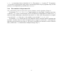
2.6.2 Output file format
The output of E2 LSH is twofold. The main results are directed to standard output (cout). The output
stream has the following format:
Query point i : found x NNs. They are:
......
......
Total time for R-NN query: y
Additional information is reported to standard error (cerr).
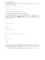
2.6.3 File with the parameters for the R-NN data structure
The file with the parameters for the R-NN data structure is the output of the bin/lsh computeParams
and the command-line parameter data set params file for the script bin/lsh fromParams. It
specifies the estimation of the optimal parameters for a spefic data set and for a specific machine. Below is
an example of such a file:
1
R
0.53
Success probability
0.9
Dimension
784
Rˆ2
0.280899972
Use <u> functions
1
k
20
m [# independent tuples of LSH functions]
35
L
595
W
4.000000000
T
9991
typeHT
3
All lines except the first one define the parameters in the following way (the first line is reserved for future use). Each odd line defines the value of a parameter (the preceding even line simply describes the name
of the corresponding parameter). The parameters R, Success Probability, Dimension, k,
m, L, W are the parameters that appear in the algorithm description (note that Success Probability,
7
k, m, L are interrelated values as described in 3.5.1). The parameter Rˆ2 is equal to R2 . The parameter
T is reserved for specifying how many points to look through before the query algorithm stops, but this
parameter is not implemented yet (and therefore is set to n).
2.6.4 The remainder of the parameter file
Note: understanding of the description below requires familarity with the algorithm of Chapter 3.
The parameter “Use <u> functions” signals whether to use the original g functions (each of the
L functions gi is a k-tuple of LSH functions; all kL LSH functions are independent) or whether to use g’s
that are not totally independent (as described in the section 3.4.1). If the value of the parameter is 0, original
g’s are used and L = m; if the value is 1, the modified g’s are used and L = m · (m − 1)/2.
The parameter typeHT defines the type of the hash table used for storing the buckets containing data
set points. Currently, values of 0 and 3 are supported, but we suggest to use the value 3. (Refering to the
hash table types described in the section 3.6, the value 0 corresponds to the linked-list version of the hash
tables, and the value 3 – to the hash tables with hybrid storage array Y .)
8
Chapter 3
Algorithm description
In this chapter, we describe first the general locality-sensitive hashing algorithm (as in [2] but with slight
modifications). Next, we gradually add more details of the algorithm as well as the optimizations in our
implementation.
3.1 Notations
We use lpd to denote the d-dimensional real space Rd under the lp norm. For any point v ∈
||v||p represents the lp norm of the vector v, that is
d
X
||v||p = (
Rd , the notation
vip )1/p
i=1
In particular ||v|| = ||v||2 is the Euclidean norm.
Let the data set P be a finite subset of Rd , and let n = |P|. A point q will usually stand for the query
point; the query point is any point from Rd . Points v, u will usually stand for some points in the data set P.
The ball of radius r centered at v is denoted by B(v, r). For a query point q, we call v an R-near
neighbor (or simply a near neighbor) if v ∈ B(q, R).
3.2 Generic locality-sensitive hashing scheme
To solve the R-NN problem, we use the technique of Locality Sensitive Hashing or LSH [4, 3]. For a domain
S of points, the LSH family is defined as:
Definition 1 A family H = {h : S → U } is called locality-sensitive, if for any q, the function p(t) =
PrH [h(q) = h(v) : ||q − v|| = t] is strictly decreasing in t. That is, the probability of collision of points q
and v is decreasing with the distance between them.
Thus, if we consider any points q, v, u, with v ∈ B(q, R) and u 6∈ B(q, R), then we have that p(||q −
v||) > p(||q − u||). Intuitively we could hash the points from P into some domain U , and then at the query
time compute the hash of q and consider only the points with which q collides.
However, to achieve the desired running time, we need to amplify the gap between the collision probabilities for the range [0, R] (where the R-near neighbors lie) and the range (R, ∞). For this purpose we concatenate several functions h ∈ H. In particular, for k specified later, define a function family G = {g : S → U k }
9
such that g(v) = (h1 (v), . . . , hk (v)), where hi ∈ H. For an integer L, the algorithm chooses L functions
g1 , . . . , gL from G, independently and uniformly at random. During preprocessing, the algorithm stores each
v ∈ P (input point set) in buckets gj (v), for all j = 1, . . . , L. Since the total number of buckets may be
large, the algorithm retains only the non-empty buckets by resorting to hashing (explained later).
To process a query q, the algorithm searches all buckets g1 (q), . . . , gL (q). For each point v found in a
bucket, the algorithm computes the distance from q to v, and reports the point v iff ||q − v|| ≤ R (v is a
R-near neighbor).
We will describe later how we choose the parameters k and L, and what time/memory bounds they give.
Next, we present our choice for the LSH family H.
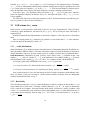
3.3 LSH scheme for lp norm
In this section, we will present the LSH family H that we use in our implementation. This LSH family
is based on p-stable distributions, that works for all p ∈ (0, 2]. We use exactly the same LSH family as
suggested by [2].
It should be noted that the implementation as described in Chapter 2 works only for the l2 (Euclidean)
norm.
Since we consider points in lpd , without loss of generality we can assume that R = 1, since otherwise,
we can scale down all the points by a factor of R.
3.3.1 p-stable distributions
Stable distributions [5] are defined as limits of normalized sums of independent identically distributed variables (an alternate definition follows). The most well-known example of a stable distribution is Gaussian (or
normal) distribution. However, the class is much wider; for example, it includes heavy-tailed distributions.
Stable Distribution: A distribution D over R is called p-stable, if there exists p ≥ 0 such that for any n real
P
numbers v1 . . . vn and i.i.d. variables X1 . . . Xn with distribution D, the random variable i vi Xi has the
P
same distribution as the variable ( i |vi |p )1/p X, where X is a random variable with distribution D.
It is known [5] that stable distributions exist for any p ∈ (0, 2]. In particular:
• a Cauchy distribution DC , defined by the density function c(x) =
1 1
π 1+x2 ,
is 1-stable
• a Gaussian (normal) distribution DG , defined by the density function g(x) =
2
√1 e−x /2 ,
2π
is 2-stable
From a practical point of view, note that despite the lack of closed form density and distribution functions, it is known [1] that one can generate p-stable random variables essentially from two independent
variables distributed uniformly over [0, 1].
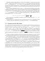
3.3.2 Hash family
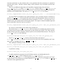
The LSH scheme proposed in [2] uses p-stable distributions as follows: compute the dot products (a.v) to
assign a hash value to each vector v. Formally, each hash function ha,b (v) : Rd → Z maps a d dimensional
vector v onto the set of integers. Each hash function in the family is indexed by a choice of random a and
b where a is a d dimensional vector with entries chosen independently from a p-stable distribution and b is
a real number chosen uniformly from the range [0, w]. For a fixed a, b the hash function ha,b is given by
ha,b (v) = ⌊ a·v+b
w ⌋
10
The intuition behind the hash functions is as follows. The dot product a.v projects each vector to the
real line. It follows from p-stability that for two vectors (v1 , v2 ) the distance between their projections
(a.v1 − a.v2 ) is distributed as ||v1 − v2 ||p X where X is a p-stable distribution. If one “chops” the real line
into equi-width segments of appropriate size w and assign hash values to vectors based on which segment
they project onto, then it is intuitively clear that this hash function will be locality preserving in the sense
described above.
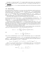
One can compute the probability that two vectors v1 , v2 collide under a hash function drawn uniformly
at random from this family. Let fp (t) denote the probability density function of the absolute value of the
p-stable distribution. We will drop the subscript p whenever it is clear from the context. For the two vectors
v1 , v2 , let c = ||v1 − v2 ||p . For a random vector a whose entries are drawn from a p-stable distribution,
a.v1 − a.v2 is distributed as cX where X is a random variable drawn from a p-stable distribution. Since b is
drawn uniformly from [0, w] it is easy to see that
p(c) = P ra,b [ha,b (v1 ) = ha,b (v2 )] =
Z
0
w
t
t
1
fp ( )(1 − )dt
c
c
w
For a fixed parameter w the probability of collision p(c) decreases monotonically with c = ||v1 − v2 ||p ,
satisfying the definition 1.
The optimal value for w depends on the data set and the query point, but it was suggested in [2] that
w = 4 provides good results, and, therefore, we currently use the value w = 4 in our implementation.
3.4 Parameters for the LSH scheme
To use LSH, we need to specify the parameters k and L. From the problem formulation, specifically from
the requirement that a near neighbor is reported with a probability at least 1 − δ, we can derive a necessary
condition on k and L. Consider a query point q and a near neighbor v ∈ B(q, R). Let p1 = p(1) = p(R).
Then, P rg∈G [g(q) = g(v)] ≥ pk1 . Thus, q and v fail to collide for all L functions gi with probability at
most (1 − pk1 )L . Requiring that the point q collides with v on some function gi is equivalent to inequation
log δ
1 − (1 − pk1 )L ≥ 1 − δ, which implies that L ≥ log(1−p
k ) . Since there are no more conditions on k and L
1
log δ
(other than minimizing the running time), we choose L = ⌈ log(1−p
k ) ⌉ (the running time is increasing with
1
L).
The value k is chosen as a function of the data set to minimize the running time of a query. Note that
this is different from the LSH scheme in [2], where k is chosen as a function of the approximation factor.
For a fixed value of k and L = L(k), we can decompose the query time into two terms. The first term
is Tg = O(dkL) for computing the L functions gi for the query point q as well as retrieving the buckets
gi (q) from hash tables. The second term is Tc = O(d · #collisions) for computing the distance to all
points encountered in the retrieved buckets. #collisions is the number of points encountered in the buckets
P
g1 (q), . . . gL (q); the expected value of #collisions is E[#collisions] = L · v∈P pk (kq − vk).
Intuitively, Tg increases as a function of k, while Tc decreases as a function of k. The latter is due to the
fact that higher values of k magnify the gap between the collision probabilities of “close” and “far” points,
which (for proper values of L) decreases the probability of collision of far points. Thus, typically there exists
an optimal value of k that minimizes the sum Tg + Tc (for a given query point q). Note that there might be
different optimal k’s for different query points, therefore the goal would be optimize the mean query time
for all query points. We discuss more on the optimization procedure in the section 3.5.1
11
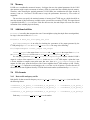
3.4.1 Faster computation of hash functions
In this section, we describe a slight modification to the LSH scheme that enables a considerable reduction
of the time Tg , the time necessary for computing the functions gi .
(i)
(i)
(i)
In the original LSH scheme, we choose L functions gi = (h1 , . . . , hk ), where each function hj is
chosen uniformly at random from the LSH family H. For a given point q, we need O(d) time to compute a
(i)
function hj (q), and O(dkL) time to compute all functions g1 (q), . . . , gL (q).
(i)
To reduce the time for computing functions gi for the query q, we reuse some of the functions hj
(in this case, gi are not totally independent). Specifically, in addition to functions gi , define functions
ui in the following manner. Suppose k is even and m is a fixed constant. Then, for i = 1 . . . m, let
(i)
(i)
(i)
ui = (h1 , . . . , hk/2 ), where each hj is drawn uniformly at random from the family H. Thus ui are
vectors each of k/2 functions drawn uniformly at random from the LSH family H.
Now, define functions gi as gi = (ua , ub ), where 1 ≤ a < b ≤ m. Note that we obtain L = m(m − 1)/2
functions gi .
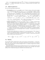
Since the functions gi are interdependent, we need to derive a different expression for the probability that
the algorithm reports a point that is within the distance R from the query point (a R-near neighbor). With
k/2 m
new functions gi , this probability is greater than or equal to 1 − 1 − p1
k/2
− m · p1
To require a success probability of at least 1 − δ, we restrict m to be such that 1 −
k/2
1 − p1
m−1
k/2 m−1
· 1 − p1
k/2 m
p1
+m·
k/2
p1
.
·
≤ δ. This inequation yields a slightly higher value for L = m(m − 1)/2 than in the case
when functions gi are independent, but L is still O
log 1/δ
pk1
√
. The time for computing the gi functions for a
query point q is reduced to Tg = O(dkm) = O(dk L) since we need only to compute m fuctions ui . The
expression for the time Tc , the time to compute the distance to points in buckets g1 (q), . . . , gL (q), remains
unchanged due to the linearity of expectation.
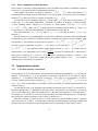
3.5 Implementation details
3.5.1 R-NN data structure construction
For constructing the R-NN data structure, the algorithm first computes the parameters k, m, L for the data
structure. The parameters k, m, L are computed as a function of the data set P, the radius R, and the
probability 1 − δ as outlined in the section 3.4 and 3.4.1. For a value of k, the parameter m is chosen
k/2 m
k/2
k/2 m−1
≤ δ; L is set to
+ m · p1 · 1 − p1
to be the smallest natural number satisfying 1 − p1
m(m − 1)/2. Thus, in what follows, we consider m and L as functions of k, and the question remains only
of how to choose k.
For choosing the value k, the algorithm experimentally estimates the times Tg and Tc as a function of k.
Remember that the time Tc is dependent on the query point q, and, therefore, for estimating Tc we need to
use a set S of sample query points (the estimation of Tc is then the mean of the times Tc for points from S).
The sample set S is chosen to be a set of several points chosen at random from the query set. (The package
also provides the option of choosing S to be a subset of the data set P.)
Note that to estimate Tg and Tc precisely, we need to know the constants hidded by the O(·) notation
in the expressions for Tg and Tc . To compute these constants, the implementation constructs a sample data
structure and runs several queries on that sample data structure, measuring the actual times Tg and Tc .
12
Concluding, k is chosen such that T˜c + Tg is minimal (while the data structure space requirement is
withinP
the memory bounds), where T˜c is the mean of the times Tc for all points in the sample query set S:
Tc (q)
T˜c = q∈S
.
|S|
Once the parameters k, m, L are computed, the algorithm constructs the R-NN data structure containing
the points from P.
3.5.2 Bucket hashing
Recall that the domain of each function gi is too large to store all possible buckets explicitly, and only nonempty buckets are stored. To this end, for each point v, the buckets g1 (v), . . . gL (v) are hashed using the
universal hash functions. For each function gi , i = 1 . . . L, there is a hash table Hi containing the buckets
{gi (v) | v ∈ P}. For this purpose, there are 2 associated hash functions h1 : Zk → {0, . . . , tableSize − 1}
and h2 : Zk → {0, . . . , C} (each gi maps to Zk ). The function h1 has the role of the usual hash function in
an universal hashing scheme. The second hash function identifies the buckets in chains.
The collisions within each bucket are resolved by chaining. When storing a bucket gi (v) = (x1 , . . . xk )
in its chain, instead of storing the entire vector (x1 , . . . xk ) for bucket identification, we store only h2 (x1 , . . . xk ).
Thus, a bucket gi (v) = (x1 , . . . xk ) has only the following associated information stored in its chain: the
identifier h2 (x1 , . . . , xk ), and the points in the bucket, which are gi−1 (x1 , . . . xk ) ∩ P.
The reasons for using the second hash function h2 instead of storing the value gi (v) = (x1 , . . . xk )
are twofold. Firstly, by using a fingerprint h2 (x1 , . . . xk ), we decrease the amount of memory for bucket
identification from O(k) to O(1). Secondly, with the fingerprint it is faster to look up a bucket in the hash
table. The domain of the function h2 is chosen big enough to ensure with a high probability that any two
different buckets in the same chain have different h2 values.
All L hash tables use the same primary hash function h1 (used to dermine the index in the hash table)
and the same secondary hash function h2 . These two hash functions have the form
k
X
h1 (a1 , a2 , . . . , ak ) =
!
!
ri′ ai mod prime mod tableSize,
i=1
and
h2 (a1 , a2 , . . . , ak ) =
k
X
ri′′ ai
i=1
!
mod prime,
where ri′ and ri′′ are random integers, tableSize is the size of the hash tables, and prime is a prime number.
In the current implementation, tableSize = |P|, ai are represented by 32-bit integers, and prime is
equal to 232 −5. This value of prime allows fast hash function computation without using modulo operations.
Specifically, consider computing h2 (a1 ) for k = 1. We have that:
h2 (a1 ) = r1′′ a1 mod 232 − 5 = low r1′′ a1 + 5 · high r1′′ a1
mod (232 − 5)
where low[r1′′ a1 ] are the low-order 32 bits of r1′′ a1 (a 64-bit number), and high[r1′′ a1 ] are the high-order
32 bits of r1′′ a1 . If we choose
ri′′ from the range [1, . . . 229 ], we will always have that α = low [r1′′ a1 ] + 5 ·
high [r1′′ a1 ] < 2 · 232 − 5 . This means that
h2 (a1 ) =
(
α
, if α < 232 − 5
32
α − 2 − 5 , if α ≥ 232 − 5
13
For k > 1, we compute progressively the sum
P
k
′′
i=1 ri ai mod prime keeping always the partial sum
modulo 232 − 5 using the same principle as the one above. Note that the range of the function h2 thus
becomes {1, . . . 232 − 6}.
3.5.3 Additional optimizations
We use the following additional optimizations.
• Precomputation of gi (q), h1 (gi (q)), and h2 (gi (q)). To answer a query, we first need to compute
gi (q). As mentioned in the section 3.4.1, since gi = (ua , ub ), we need only to compute k/2-tuples
ua (q), a = 1, . . . m. Further, for searching for buckets gi (q) in hash tables, we need in fact only
h1 (gi (q)) and h2 (gi (q)). Precomputing h1 and h2 in the straight-forward way would take O(Lk)
time. However, since gi are of the form (ua , ub ), we can reduce this time in the following way. Note
P
that each function hj , j ∈ {1, 2}, is of the form hj (x1 , . . . xk ) = (( kt=1 rij xi )mod Aj )mod Bj .
Pk
Pk/2 j
Therefore, hj (x1 , . . . xk ) may be computed as (( t=1 rt xt + t=k/2+1 rtj xt )mod Aj )mod Bj . If
j
j
, . . . rkj ), then we have that hj (gi (q)) = ((rjleft ·
), and rjright = (rk/2+1
we denote rjleft = (r1j , . . . rk/2
ua (v) + rjright · ub (v))mod Aj )mod Bj . Thus, it suffices to precompute only rjside · ua (v), where
j ∈ {1, 2}, side ∈ {lef t, right}, a ∈ {1, . . . m}, which takes O(km) time.
• Skipping repeated points. In the basic query algorithm, a point v ∈ P might be encountered more
than once. Specifically, a point v ∈ P might appear in more than one of the buckets g1 (q), . . . gL (q).
Since there is no need to compute the distance to any point v ∈ P more than once, we keep track
of the points for which we already computed the distance ||q − v||, and not compute the distance a
second time. For this purpose, for each particular query, we keep a vector ei , such that ei = 1 if we
already encountered the point vi ∈ P in an earlier bucket (and computed the distance ||q − v||), and
ei = 0 otherwise. Thus, the first time we encounter a point v in the buckets, we compute the distance
to it, which takes O(d) time; for all subsequent times we encounter v we spend only O(1) time (for
checking the vector ei ).
Note that with this optimization, the estimation of Tc is not accurate anymore. This is because Tc
is the time for computing the distance to points encountered in the buckets g1 (q), . . . gL (q). Taking
into the consideration only the distance computations (i.e., assuming we spend no time on subsequent
copies of a point), the new expression for Tc is
E[Tc ] = d ·
X
v∈P
k/2
1 − 1 − p(||q − v||)
m
k/2
− m · p(||q − v||)
k/2
· 1 − p(||q − v||)
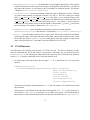
m−1 3.6 Memory
The R-NN data structure described above requires O(nL) memory (for each function gi , we store the n
points from P). Since, L increases with k, the memory requirement is big for big data set or for moderate
data set for which optimal time is achived with higher values of k. Therefore, an upper limit on memory
imposes an upper limit on k.
Because the memory requirement is big, the constant in front of O(nL) is very important. In our current
implementation, with the best variant of the hash tables, this constant is 12 bytes. Note that it is the structure
and layout of the L hash tables that plays the substantial role in the memory usage.
14
Below we show two variants of the layout of the hash tables that we deployed. We assume that 1) the
number of points is n ≤ 220 ; 2) each pointer is 4 bytes long; 3) tableSize = n for each hash table.
One of the most straightforward layouts of a hash table Hi is the following. For each index l of the hash
table, we store a pointer to a singly-linked list of buckets in the chain l. For each bucket, we store its value
h2 (·), and a pointer to a singly-linked list of points in the bucket. The memory requirement per hash table is
4 · tableSize + 8 · #buckets + 8 · n ≤ 20n, yielding a constant of 20.
To reduce this constant to 12 bytes, we do the following. Firstly, we index all points in P, such that
we can refer to points by index (this index is constant across all hash tables). Refering to a point thus takes
only 20 bits (and not 32 as in the case of a pointer). Consider now a hash table Hi . For this hash table,
we deploy a table Y of 32-bit unsigned integers that store all buckets (with values h2 (·)) and points in the
buckets (thus, Y is a hybrid storage table since it stores both buckets’ and points’ description). The table
has a length of #buckets + n and is used as follows. In the hash table Hi , at index l, we store the pointer
to some index el of Y ; el is the start of the description of the chain l. A chain is stored as follows: h2 (·)
value of the first bucket in chain (at position el in Y ) followed by the indeces of the points in this bucket
(positions el + 1, . . . el + n1 ); h2 (·) value of the second bucket in the chain (position el + n1 + 1) followed
by the indeces of the points in this second bucket (positions el + n1 + 2, . . . el + n1 + 1 + n2 ); and so forth.
Note that we need also to store the number of buckets in each chain as well as the number of points in
each bucket. Instead of storing the chain length, we store for each bucket a bit that says whether that bucket
is the last one in the chain or not; this bit is one of the unused bits of the 4-byte integer storing the index of
the first point in the corresponding bucket (i.e., if the h2 (·) value of the bucket is stored at position e in Y ,
then we use a high-order bit of the integer at position e + 1 in Y ). For storing the length of the bucket, we
use the remaining unused bits of the first point in the bucket. When the remaining bits are not enough (there
are more than 232−20−1 − 1 = 211 − 1 points in the bucket), we store a special value for the length (0),
which means that there are more than 211 − 1 points in the bucket, and there are some additional points (that
do not fit in the 211 − 1 integers alloted in Y after the h2 (·) value of the bucket). These additional points
are also stored in Y but at a different position; their start index and number are stored in the unused bits of
the remaining 211 − 2 points that follow the h2 (·) value of the bucket and the first point of the bucket (i.e.,
unused bits of the integers at positions e + 2, . . . e + 211 − 1).
3.7 Future possible optimizations
• Parameter w of the LSH scheme. In addition to optimizing k, the algorithm could optimize the
parameter w to achieve the best query time. The function p depends on the parameter w, and, thus,
both times Tc and Tg depend on w. Currently, we use a fixed value of 4, but the optimal value of w is
a function of the data set P (and a sample query set).
• Generalization of functions gi = (ua , ub ). In section 3.4.1 we presented a new approach to choosing
functions gi . Specifically, we choose functions gi = (ua , ub ), 1 ≤ a < b ≤ m, where each uj ,
j = 1 . . . m, is a k/2-tuple of random independent hash functions from the LSH family H.
√ In this
way, we decreased the time to compute functions gi (q) for a query q from O(dkL) to O(dk L).
This approach could be generalized to functions g that are t-tuples of functions u, where u are drawn
indepently from Hk/t , reducing in this way the asymptotic time
computing the functions g. We
for did not pursue this generalization since, even if L is still O
log 1/δ
pk1
, the constant hidden by O(·)
notation for t > 2 would probably nullify the theoretical gain for the typical data sets.
15
Chapter 4
The E2LSH Code
4.1 Code overview
The core of the E2 LSH code is divided into three main components:
• LocalitySensitiveHashing.cpp – contains the implementation of the main LSH-based Rnear neighbor data strucure (except the hashing of the buckets). The main functionality is for constructing the data structure (given the parameters such as k, m, L), and for answering a query.
• BucketHashing.cpp – contains the implementation of the hash tables for the universal hashing
of the buckets. The main functionality is for constructing hash tables, adding new buckets/points to
it, and looking-up a bucket.
• SelfTuning.cpp – contains functions for computing the optimal parameters for the R-near neighbor data structure. Contains all the functions for estimating the times Tc , Tg (including the functions
for estimating #collisions).
Additional code making part of the core is contained in the following files:
• Geometry.h – contains the definition for a point (PPointT data type);
• NearNeighbors.cpp, NearNeighbors.h – contain the functions at the interface of the E2 LSH
core (see a more detailed description below);
• Random.cpp, Random.h – contain the pseudo-random number generator;
• BasicDefinitions.h – contains the definitions of general-purpose types (such as, IntT, RealT)
and macros (such as the macros for timing operations);
• Utils.cpp, Utils.h – contain some general purpose functions (e.g., copying vectors).
Another important part of the package is the file LSHMain.cpp, which is a sample code for using
E2 LSH. LSHMain.cpp only reads the input files, parses the command line parameters, and calls the corresponding functions from the package.
The most important data structures are:
16
• RNearNeighborStructureT – the fundamental R-near neighbor data structure. This structure
contains the parameters used to construct the structure, the description of the functions gi , the index of
the points in the structure, as well pointers to the L hash tables for storing the buckets. The structure
is defined in LocalitySensitiveHashing.h.
• UHashStructureT – the structure defining a hash table used for hashing the buckets. Collisions
are resolved using chaining as explained in sections 3.5.2 and 3.6. There are 2 main types of hash
tables: HT LINKED LIST and HT HYBRID CHAINS (the field typeHT contains the type of the
hash table). The type HT LINKED LIST corresponds to the linked-list version of the hash table, and
HT HYBRID CHAINS – to the one with hybrid storage array Y (see section 3.6 for more details).
Each hash table also contains pointers to the descriptions of the functions h1 (·) and h2 (·) used for the
universal hashing. The structure is defined in BucketHashing.h.
• RNNParametersT – a struct containing the parameters necessary for constructing the
RNearNeighborStructureT data structure. It is defined in LocalitySensitiveHashing.h.
• PPoint – a struct for storing a point from P or a query point. This structure contains the coordinates
of the point, the square of the norm of the point, and an index, which can be used by the callee outside
the E2 LSH code (such as LSHMain.cpp) for identifying the point (for example, it might by the
index of the point in the set P); this index is not used within the core of E2 LSH.
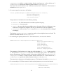
4.2 E2LSH Interface
The following are the functions at the interface of E2 LSH core code. The first two functions are sufficient for constructing the R-NN data structure, and querying it afterwards; they are declared in the file
NearNeighbors.h. The following two functions provide a separation of the estimation of the parameter
(such as k, m, L) from the construction of the R-NN data structure itself.
1. To construct the R-NN data structure given as input 1 − δ, R, d, and the data set P, one can use the
function
PRNearNeighborStructT
initSelfTunedRNearNeighborWithDataSet(RealT thresholdR,
RealT successProbability,
Int32T nPoints,
IntT dimension,
PPointT *dataSet,
IntT nSampleQueries,
PPointT *sampleQueries)
The function will estimate optimal parameters k, m, L, and will construct a R-NN data structure from
this parameters.
The parameters of the function are the input data of the algorithm: R, 1 − δ, n, d, and respectively P.
The parameter sampleQueries represents a set of sample query points – the function optimizes
the parameters of the constructed data structure for the points specified in the set sampleQueries.
17
sampleQueries could be a sample of points from the actual query set or from the data set P.
nSampleQueries specifies the number of points in the set sampleQueries.
The return value of the function is the R-NN data structrure that is constructed. This function is
declared in NearNeighbors.h.
2. For a query operation, one can use the function
Int32T getRNearNeighbors(PRNearNeighborStructT nnStruct,
PPointT queryPoint,
PPointT *(&result),
IntT &resultSize)
The parameters of the function have the following meaning:
• nnStruct – the R-NN data structure on which to perform the query;
• queryPoint – the query point;
• result – the array where the near neighbors are to be stored (if the size of this array is not
sufficient for storing the near neighbors, the array is reallocated to fit all near neighhbors);
• resultSize – the size of the result array (if the result is resized, this value is changed
accordingly);
The function getRNearNeighbors returns the number of near neighbors that were found. The
function is declared in the file NearNeighbors.h.
3. For estimating the optimal parameters for a R-NN data structure, one can use the function
RNNParametersT computeOptimalParameters(RealT R,
RealT successProbability,
IntT nPoints,
IntT dimension,
PPointT *dataSet,
IntT nSampleQueries,
PPointT *sampleQueries)
The parameters of the function are the input data of the algorithm: R, 1 − δ, n, d, and respectively
P. The parameter sampleQueries represents a set of sample query points – the function optimizes the parameters of the data structure for the points specified in the set sampleQueries.
sampleQueries could be a sample of points from the actual query set or from the data set P.
nSampleQueries specifies the number of points in the set sampleQueries.
The return value is the structrure with optimal parameters. This function is declared in SelfTuning.h.
4. For constructing the R-NN data structure from the optimal parameters, one can use the function
PRNearNeighborStructT initLSH_WithDataSet(RNNParametersT algParameters,
Int32T nPoints,
PPointT *dataSet)
18
algParameters specify the parameters with which the R-NN data structure will be constructed.
The function returns the constructed data structure. The function is declared in
LocalitySensitiveHashing.h.
19
Chapter 5
Frequent Anticipated Questions
In this section we give answers to some questions that the reader might ask when compiling and using the
package.
1. Q: How to compile this thing ?
A: Since you are reading this manual, you must have already gunzipped and untarred the original file.
Now it suffices to type make in the main directory to compile the code.
2. Q: OK, it compiles. Now what ?
A: You can run the program on a provided data set mnist1k.dts and query set mnist1k.q. They
reside in the main directory. Simply type
bin/lsh 0.6 mnist1k.dts mnist1k.q >o
This will create an output file o containing the results of the search. To see if it worked, run the exact
algorithm
bin/exact 0.6 mnist1k.dts mnist1k.q >o.e
and compare the outputs by running
bin/compareOutputs o.e o
You should receive an answer that looks like:
Overall: OK = 1. NN_LSH/NN_Correct = 5/5=1.000
This means that the run was “OK”, and that the randomized LSH algorithm found 5 out of 5 (i.e., all)
near neighbors within distance 0.6 from the query points. Note that, since the algorithm is randomized,
your results could be different (e.g., 4 out of 5 near neighbors). However, if you are getting 0 out of
5, then probably something is wrong.
20
3. Q: I ran the code, but it is so slow!
A: If the code is unusually slow, it might mean two things:
• The code uses so much memory that the system starts swapping. This typically degrades the
performance by 3 orders of magnitude, so should be definitely avoided. To fix it, specify the
amount of available (not total) memory in the file bin/mem.
• The search radius you specified is so large that many/most of the data points are reported as near
neighbors. If this is what you want, then the code will not run much faster. In fact, you might be
better off using linear scan instead, since it is simpler and has less overhead.
Otherwise, try to adjust the search radius so that, on average, there are few near neighbors per
query. You can use bin/exact for experiments, it is likely to be faster than LSH if you
perform just a few queries.
21
Bibliography
[1] J. M. Chambers, C. L. Mallows, and B. W. Stuck. A method for simulating stable random variables. J.
Amer. Statist. Assoc., 71:340–344, 1976.
[2] M. Datar, N. Immorlica, P. Indyk, and V. Mirrokni. Locality-sensitive hashing scheme based on p-stable
distributions. DIMACS Workshop on Streaming Data Analysis and Mining, 2003.
[3] A. Gionis, P. Indyk, and R. Motwani. Similarity search in high dimensions via hashing. Proceedings of
the 25th International Conference on Very Large Data Bases (VLDB), 1999.
[4] P. Indyk and R. Motwani. Approximate nearest neighbor: towards removing the curse of dimensionality.
Proceedings of the Symposium on Theory of Computing, 1998.
[5] V.M. Zolotarev. One-Dimensional Stable Distributions. Vol. 65 of Translations of Mathematical Monographs, American Mathematical Society, 1986.
22