Download A User's Guide to Zot

A User’s Guide to Zot
June 2013
CONTENTS
i
Contents
1 Overview
1
2 Installation
2.1 Hello world . . . . . . . . . . . . . . . . . . . . . . . . . . . .
2
2
3 Languages
3.1 CLTLB . . . . . . . .
3.2 Quantifiers . . . . . .
3.3 Short examples . . . .
3.4 PLTL . . . . . . . . .
3.5 TRIO . . . . . . . . .
3.6 Operational constructs
3.7 MTL . . . . . . . . . .
3.8 Timed Automata . . .
.
.
.
.
.
.
.
.
.
.
.
.
.
.
.
.
.
.
.
.
.
.
.
.
.
.
.
.
.
.
.
.
.
.
.
.
.
.
.
.
.
.
.
.
.
.
.
.
.
.
.
.
.
.
.
.
.
.
.
.
.
.
.
.
.
.
.
.
.
.
.
.
.
.
.
.
.
.
.
.
.
.
.
.
.
.
.
.
.
.
.
.
.
.
.
.
.
.
.
.
.
.
.
.
.
.
.
.
.
.
.
.
.
.
.
.
.
.
.
.
.
.
.
.
.
.
.
.
.
.
.
.
.
.
.
.
.
.
.
.
.
.
.
.
.
.
.
.
.
.
.
.
.
.
.
.
.
.
.
.
.
.
.
.
.
.
.
.
.
.
.
.
.
.
.
.
6
7
8
9
10
10
11
13
13
4 Usage
4.1 SAT-solvers . . . . . .
4.2 SMT-solvers . . . . . .
4.3 Model Checking . . . .
4.4 Completeness . . . . .
4.5 Satisfiability Checking
4.6 Temporary data . . .
.
.
.
.
.
.
.
.
.
.
.
.
.
.
.
.
.
.
.
.
.
.
.
.
.
.
.
.
.
.
.
.
.
.
.
.
.
.
.
.
.
.
.
.
.
.
.
.
.
.
.
.
.
.
.
.
.
.
.
.
.
.
.
.
.
.
.
.
.
.
.
.
.
.
.
.
.
.
.
.
.
.
.
.
.
.
.
.
.
.
.
.
.
.
.
.
.
.
.
.
.
.
.
.
.
.
.
.
.
.
.
.
.
.
.
.
.
.
.
.
.
.
.
.
.
.
.
.
.
.
.
.
15
15
15
15
21
23
25
5 Architecture
26
5.1 PLTL-to-SAT encodings . . . . . . . . . . . . . . . . . . . . . 26
5.2 Main Interface . . . . . . . . . . . . . . . . . . . . . . . . . . 27
5.3 Other modules and plug-ins . . . . . . . . . . . . . . . . . . . 29
1
1
OVERVIEW
1
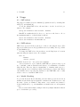
Overview
Zot is an agile and easily extendible bounded model checker, which can be
downloaded at http://home.dei.polimi.it/pradella/.
The tool supports different logic languages through a multi-layered approach: its core uses CLTLB(DL)[6] and on top of it a decidable predicative
fragment of TRIO [14] is defined. An interesting feature of Zot is its ability
to support different encodings of temporal logic as SMT problems by means
of plug-ins. This approach encourages experimentation, as plug-ins are expected to be quite simple, compact (usually around 500 lines of code), easily
modifiable, and extendible. At the moment, a variant of the eventuality encoding presented in [8] is supported, (approximated) dense-time MTL [11],
and a bi-infinite encoding [18], [19].
Zot offers three basic usage modalities:
1. Bounded satisfiability checking (BSC): given as input a specification
formula, the tool returns a (possibly empty) history (i.e., an execution
trace of the specified system) which satisfies the specification. An
empty history means that it is impossible to satisfy the specification.
2. Bounded model checking (BMC): given as input an operational model
of the system, the tool returns a (possibly empty) history (i.e., an
execution trace of the specified system) which satisfies it.
3. History checking and completion (HCC): The input file can also contain a partial (or complete) history H. In this case, if H complies with
the specification, then a completed version of H is returned as output,
otherwise the output is empty.
The provided output histories have temporal length ≤ k, the bound
given by the user, but may represent infinite behaviors thanks to the loop
selector variables, marking the start of the periodic sections of the history.
The BSC/BMC modalities can be used to check if a property prop of the
given specification spec holds over every periodic behavior with period ≤ k.
In this case, the input file contains spec ∧ ¬prop, and, if prop indeed holds,
then the output history is empty. If this is not the case, the output history
is a counterexample, explaining why prop does not hold.
2
INSTALLATION
2
2
Installation
Zot’s core is written in Common Lisp (with ASDF packaging http://www.cliki.net/asdf). It can be used under Linux, Windows, or MacOS X, but
has been tested only under Linux and Windows XP, using the following
Common Lisps1 :
• SBCL (http://www.sbcl.org),
• CLISP (http://clisp.cons.org),
• CMUCL (http://www.cons.org/cmucl/),
• ABCL (http://common-lisp.net/project/armedbear/),
• Clozure CL (http://www.clozure.com/clozurecl.html),
This approach makes Zot an open system, as it uses Common Lisp also as
internal scripting language of the tool, both to define complex verification
activities, and to add new constructs and languages on top of the existing
ones.
Typically, to install Zot in a Debian system (or Ubuntu), the user must
install a Common Lisp (e.g. one of the packages clisp, sbcl, cmucl,
. . . ), and the common-lisp-controller package. To perform a systemwide install of the Zot packages, just put symbolic links to its .ads files in
the /usr/share/common-lisp/systems/ directory. Note that it is possible to
avoid a system-wide installation, but in this case the user has to work inside
the main Zot directory.
Zot works with external SAT-solvers. The supported SAT-solvers are
MiniSat (default) [9], MiraXT [15], PicoSAT [7], and zChaff [16]. Zot assumes that executable files called minisat, MiraXTSimp (optional), picosat
(optional), zchaff (optional), are system-wide installed.
A pre-packaged all-inclusive version for Windows (WinZot, based on
Cygwin-compiled binaries and SBCL) is available from the author.
All Zot’s components are available as open source software (GPL v2).
2.1
Hello world
Here, the user can find short examples of the functionality of Zot which can
be used to test the installation and to understand the basic notion supporting the tool (knowledge about verification and bounded model checking are
hardly recommended).
Zot is tailored to solve the Bounded Model Checking problem (BMC)
and Bounded Satisfiability Checking (BSC) which are both reduced to a
satisfiability problem. The aim of the satisfiability process is to represent
1
SBCL and CMUCL are usually the fastest implementations, for running Zot.
2
INSTALLATION
3
infinite model of CLTLB/LTL formulae by means of a finite representation of
length k (i.e., k instant of time). A model is an infinite word of propositional
atoms (and counters’ values when CLTLB is considered). In the following
sections, the term model and behavior (of a system), in particular when the
satisfiability checking is performed, have the same meaning and they can be
equivalently used.
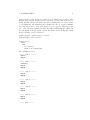
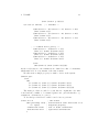
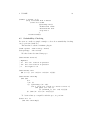
The first example shows how to solve the BSC for a LTL formula by
means of a finite representation of its model of length 5.
(asdf:operate ’asdf:load-op ’eezot)
(use-package :trio-utils)
(eezot:zot 5
(&& (-P- Hello)
(next (-P- world))))
The first two lines load the plugin eezot for LTL and the basic definitions of
operators available from trio-utils.lisp. The Common Lisp function zot
of the package eezot is invoked with the length of the (finite) model and the
LTL formula to be satisfied. The output reported is the model satisfying the
LTL formula hello ∧ Xworld (hello holds in the origin instant and world
in the next one).
------ time 0 -----WORLD
------ time 1 -----HELLO
WORLD
------ time 2 -----HELLO
WORLD
------ time 3 ----------- time 4 ----------- time 5 ----------- end -----The formula is evaluated in 1, which is the origin of the model; the instant
0 is defined for technical reasons. It is worth noticing that predicate hello
holds in 1 and world holds in 2. If no formula defines the truth value of
2
INSTALLATION
4
generic subset of the atomic propositions (or formulae) for a generic time
instant, then, in that instant, it may, or may not, holds; this is the case of
world which holds in 1 and hello in 2. The resulting finite model is a prefix
of all infinite models satisfying the formula since the proposition *LOOP*,
denoting the position of the periodicity, does not appear. This is not the
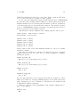
case of the following example in which the LTL formula G(hello ∧ Xworld)
(for all instant from the origin towards the future, hello holds and world
in the following one) is considered:
(asdf:operate ’asdf:load-op ’eezot)
(use-package :trio-utils)
(eezot:zot 5
(alwf
(&&
(-P- hello)
(next (-P- world)))))
the resulting model is:
------ time 0 -----HELLO
WORLD
------ time 1 -----**LOOP**
HELLO
WORLD
------ time 2 -----HELLO
WORLD
------ time 3 -----HELLO
WORLD
------ time 4 -----HELLO
WORLD
------ time 5 -----HELLO
WORLD
------ end ------
2
INSTALLATION
5
The LTL operator G is written as alwf (always in the future) and the
symbol && is the usual ∧ boolean connective. The finite model represents
the infinite periodic model given by the ω-regular expression
({h, w}, {h, w}, {h, w}, {h, w}, {h, w})ω ,
where h, w are shorthands for hello and world, respectively.
Let consider the following example in which it is shown an unsatisfiable
LTL formula G(hello ∧ Xworld) ∧ F(¬hello):
(asdf:operate ’asdf:load-op ’eezot)
(use-package :trio-utils)
(eezot:zot 5
(&&
(alwf
(&&
(-P- hello)
(next (-P- world))))
(somf (!! (-P- hello)))))
The output is, clearly:
---------UNSAT--------The operator somf corresponds to the LTL operator F and means “eventually in the future”.
3
LANGUAGES
3
6
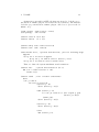
Languages
Being an open system, Zot supports different languages. At present, the
main native language is CLTLB[6] (linear temporal logic with future and
past operators over constraint systems) and its subclasses. The other main
layer based on PLTL is the metric temporal logic TRIO.
Zot scripts are interpreted as a usual Lisp code2 . Beside the CLTLB
temporal operators and relations/functions available from the constraints
system used (Difference Logic, Linear Integer Arithmetic), the user can define own constructs and embeds them in the CLTLB formulae. These constructs are defined accordingly to Common Lisp language. They are firstly
interpreted by the Common Lisp interpreter and the results is used to define
the CLTLB formulae. Here, a short list of useful constructs of the Common
Lisp language is provided.
Constants: a Lisp constant c of value v is declared in the following way:
(defconstant c v)
Variables: a Lisp variable v is declared in the following way:
(defvar v 1)
(defvar v ’(One Two))
Note that the value of a constant or a variable can be any Common Lisp object including CLTLB formula (since they are Common Lisp list), as shown
later in the section 3.3.
Functions: an n-ary Lisp function f un of domain is defined as:
(defun fun (x_1 ... x_n) axioms )
where axioms describe the properties of f un. The user should consider these
functions as procedure and should not confuse them with a CLTLB unintepreted function/relation, defined in the following section. At the end of
the section, after the definition of of the syntax of CLTLB, a simple example
is provided.
Valuation of a function: if f un is an n-ary Lisp function, the value
f un(x1 , . . . , xn ) is written as (fun x_1 ... x_n).
Predefined operation and relations: a small number of binary operation/relations between integer are predefined in Common Lisp, namely =,
\=, <, <=, >, >=, +, -, with their usual meanings:
(op x_1 x_2);
2
A basic knowledge of the language is required. It is very easy to find online a lot of
tutorials and short presentations, e.g., http://gigamonkeys.com/book/
3
LANGUAGES
3.1
7
CLTLB
CLTLB (Counters LTL)3 is, essentially, Propositional LTL with both future
and past operators (PLTLB), with in addition terms that are arithmetic
constraints in Integer Difference Logic, CLTLB(DL), or in Linear Integer
Arithmetic, CLTLB(LIA).
Propositional operators: are written as !! (not), && (and), || (or), ->
(implies) and <-> (equivalent).
Propositional letters: a proposition Q is written (-P- Q).
Relations: there exist two possible way to define a relation.
1. Uninterpreted time-variant relations: an uninterpreted (i.e. satisfying
no axioms) time-variant relations (i.e. varying in time) rel on the set
type1 × · · · × typen is defined as
(define-tvar rel *type_1* ... *type_n*)
2. Uninterpreted time-invariant relations: an uninterpreted (i.e. satisfying no axioms) time-invariant relations (i.e. constant in time) rel on
the set type1 × · · · × typen is defined as
(define-var rel *type_1* ... *type_n*)
Time-variant/unvariant variables are defined as 0-ary relations. The domains specified as *type_i* are, actually, the ones supported by the used
SMT-solver. Available keywords are: one to define Integers, *int*, one to
define Reals, *real* and *bool* to define Boolean (supported in Z3).
Valuation of a predicate: if R is an n-ary relation, the boolean R(x1 , . . . , xn )
is written as (-V- R x1 ... xn).
Valuation of a variable: a variable is evaluated differently depending on
if it is a Lisp variable or a 0-ary function:
• if var is a Lisp variable, its value is written as a usual Lisp variable;
• if var is a logic variable, its value is written as (-V- var).
Predefined operation and relations: a small number of binary operation/relations between integers are predefined in the SMT-library, namely
3
only available in the plugin ae2zot
3
LANGUAGES
8
=, <, <=, >, >=, +, -, % with their usual meanings (% is the remainder operator). As CLTLB operations (which map to SMT-LIB operations) they are
written:
([op] x_1 x_2).
Observe that some operations are not defined in all constraint systems: in
order to use + and − the logic QF_UFLIA has to be declared.
Arithmetic temporal terms: if α is an arithmetic temporal term, Xα and
Yα are written respectively as (next (-V- alpha)) and (yesterday (-V- alpha)).
Temporal operators: the following temporal operators are supported:
until, since, release, trigger, next, yesterday, zeta. The last one is
the dual of yesterday, and is used only in the mono-infinite semantics.
For the semantics of these operators, see e.g. [6]. TRIO operator are
also supported, see section 3.5
3.2
Quantifiers
Quantification is possible over finite and infinite domains (in the second case
undecidability problems can arise). Finite domains can be declared as Lisp
list:
(defvar Set ’(One Two))
The formula ∃t ∈ Set : F ormula(t) is written
(-E- t Set (Formula t)).
The definition of the Lisp variable Set is optional, and the same formula
can be written as:
(-E- t ’(One Two) (Formula t)).
-A- is the universal quantifier.
Infinite domains are implicitly declared by the definition of the constraint system. Available domains from SMT-LIB are Integers and Reals.
By the definition of satisfiability, all logic variables (as well as values of
uninterpreted functions and predicates) are existentially quantified. The
formula ∃t ∈ Z : F ormula(t) requires the definition of a logic variable by
(define-var h *int*) or (define-var h *real*) and it is written:
(Formula (-V- h)).
by simply substituting the instance of t with the evaluation of (-V- h).
3
LANGUAGES
9
It is worth noticing that the Naturals can be defined by constraining
the value of the existentially quantified variable. The formula ∃t ∈ N :
F ormula(t) can be written:
(&& ([>=] (-V- h) 0) (Formula (-V- h))).
and Formula should be defined by the construct defun. The first form,
which uses the Lisp definition of sets as lists, can be equivalently written by
using logic variables; values of a variable over a finite set are defined by an
explicit list:
(&& (|| ([=] (-V- h) c_0) ([=] (-V- h) c_1) ...)
(Formula (-V- h))).
3.3
Short examples
Some simple examples of compound syntax of CLTLB and Common Lisp
are here shown.
(defconstant p
(<->
(until (-P- A) ([>] (-V- x) 0))
(!! (-P- B))))"
The following function is useful to define the transition from the value 1 to
0 of an arithmetic temporal term.
(defun g (z)
(&& ([=] z 0) (yesterday ([=] z 1))))
The definition of g is realized by combining CLTLB language and Common
Lisp language. During the process of evaluation of the function, the variable
z is substituted with its evaluation. The function has to be used accordingly
to the syntax defined by the declared formula. In this case, the variable z
is an arithmetic temporal term Xj x; a correct use is, for example:
(<-> (-P- A) (g (next (-V- y)))))
where the variable y is a CLTLB variable defined by using the construct
define-tvar.
The following example makes use of two uninterpreted function A and B and
quantification over finite domains (-A- ...) and (-E- ...).
(define-tvar A *int* *int* *int*)
(define-tvar B *int* *int*)
(defconstant f
3
LANGUAGES
10
(-A- x ’(1 2 3)
(-A- y ’(1 2 3)
(alwf
(->
(&& ([!=] x y) ([>=] (-V- A x y) 0))
([=] (next (-V- A x y)) ([+] (-V- A x y) (-V- B x)))))))
...
3.4
PLTL
PLTL is a subclass of CLTLB in which no relations, functions and variables
appear. Nevertheless variables over finite domains can still be used (actually
this is only a useful shorthand). If the problem is expressed in PLTL there
is no need to declare a costraint system.
The following temporal operators are supported: until, since, release,
trigger, next, yesterday, zeta. The last one is the dual of yesterday,
and is used only in the mono-infinite semantics.
For the semantics of these operators, see e.g. [6] or any other note about
LTL.
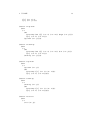
3.5
TRIO
Zot was originally born as a satisfiability checker for the TRIO metric temporal logic [14].
The list of supported operators (and their correct “Zot spelling”) is the
following:
dist
futr
past
lasts
lasted
withinf
withinp
lasttime
nexttime
somf
somp
alwf
alwp
until
since
lasts_ee
lasted_ee
withinf_ee
withinp_ee
lasttime_ee
nexttime_ee
somf_e
somp_e
alwf_e
alwp_e
until_ie
since_ie
lasts_ie
lasted_ie
withinf_ie
withinp_ie
lasttime_ie
nexttime_ie
somf_i
somp_i
alwf_i
alwp_i
until_ee
since_ee
lasts_ei
lasted_ei
withinf_ei
withinp_ei
lasttime_ei
nexttime_ei
som
lasts_ii
lasted_ii
withinf_ii
withinp_ii
lasttime_ii
nexttime_ii
alw
until_ii
since_ii
Bounded version of since and until are written as:
until_ei
since_ei
3
LANGUAGES
11
(until_ie_<=_<= t1 t2 A B)
B will be true at t instants in the future with t1<=t<=t2
(until_ie_>= t1 A B)
B will be true at t instants in the future with t>=t1
since_ie_<=_<=
since_ie_>=
Caveat emptor! The default until is PLTL’s (which is usually called
until_ie in TRIO). For example, the following model satisfies (until A B)
at 0:
0
B
---------------------AAAAAAAAAAAAAAAAAAAAA
B may appear at 0.
For MTL users:
1. ♦=t A (or =t A)) is written (futr (-P- A) t);
2. ≤t A is written (lasts (-P- A) t);
3. ♦≤t A is written (withinf (-P- A) t);
4. =t A (or =t A)) is written (past (-P- A) t);
5. ≤t A is written (lasted (-P- A) t);
6. ≤t A is written (withinp (-P- A) t);
with t > 0.
3.6
Operational constructs
Zot offers some simple facilities to describe operational systems. The following constructs are represented by means of a propositional encoding and,
therefore, they are available both for SAT-based plug-in, e.g., eezot, and for
SMT-based plug-in, ae2zot.
(define-item
<varname> <domain>)
is used to define variables `
a la Von Neumann over finite domains (e.g. counters).
(define-array <varname> <index-domain> <domain>)
is used to define mono-dimensional arrays.
Example usage:
3
LANGUAGES
12
(define-item cont (loop for i from 0 to 9 collect i))
(define-array arr (loop for i from 0 to 9 collect i)
’(on off unknown))
In the spec, the user can e.g. write (cont= 6); (arr= 6 ’off).
Caveat: both define-item and define-array have side effects. It is therefore wrong to “define-items” after a zot main procedure call, since successive
calls may work with spurious constraints. It is therefore recommended to
perform (clean-up) before defining items or arrays.
Typically, to define an operational model means to constraint operational
variables and arrays. This can be done either by using simple next-time
formulae, i.e. containing only the next temporal operator, or by using the
two dual constructs and-case and or-case [20].
To give the reader an idea of their semantics, here is an automatic translation made by Zot on two simple examples.
(and-case (x ’(1 2) y ’(3 4))
((-P- P x) (-P- Q x))
((-P- R y) (-P- R1 y))
(else (-P- R2 x)))
expands to
(-A- X ’(1 2)
(-A- Y ’(3 4)
(&& (-> (-P- R Y) (-P- R1 Y)) (-> (-P- P X) (-P- Q X))
(-> (&& (!! (-P- R Y)) (!! (-P- P X))) (-P- R2 X)))))
and
(or-case (x ’(1
((-P((-P(else
2) y
P x)
R y)
(-P-
’(3 4))
(-P- Q x))
(-P- R1 y))
R2 x)))
expands to
(-E- X ’(1 2)
(-E- Y ’(3 4)
(|| (&& (-P- R Y) (-P- R1 Y)) (&& (-P- P X) (-P- Q X))
(&& (!! (-P- R Y)) (!! (-P- P X)) (-P- R2 X)))))
3
LANGUAGES
3.7
13
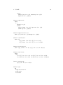
MTL
There is an experimental plug-in (called ap-zot for using a variant of densetime MTL through approximation (see [11], and [10]). Observe that MTL
is a pure propositional temporal logic, so relations, functions and variables
over possible infinite domains are not supported.
Here is a list of the time operator defined in ap-zot.
until-b
since-b
release-b
trigger-b
until-b-v
since-b-v
release-b-^
trigger-b-^
until-b-inf
since-b-inf
release-b-inf
trigger-b-inf
diamond
diamond-p
box
box-p
until-b-^
since-b-^
release-b-v
trigger-b-v
until-b-v-inf
since-b-v-inf
release-b-^-inf
trigger-b-^-inf
until-b-^-inf
since-b-^-inf
release-b-v-inf
trigger-b-v-inf
diamond-inf
diamond-inf-p
box-inf
box-inf-p
The plug-in offers the following operations
normalize
basicize
compute-granularity
over-approximation
under-approximation
nth-divisor
To compute over- and under-approximations, an axiom must be prepared
through the two functions basicize and normalize
(e.g. with (setf ax1 (normalize (basicize ax1)))).
The two functions over-approximation and under-approximation are used
to compute the approximated formulae, while compute-granularity is used
to set the ρ parameter (see [11] for details).
The interested reader may find a complete example in coffee.lisp.
3.8
Timed Automata
Timed Automata (TA) are supported through a very experimental plug-in
called ta-zot (see [12], [13]), which is based on the approximations offered
by ap-zot. As for ap-zot only the pure propositional version is supported.
First, here is a list of the added operators, and approximations procedures:
3
LANGUAGES
14
white-tri
white-tri/3
black-tri
black-tri/3
timed-automaton-under-formula
timed-automaton-over-formula
timed-automata-under-formula
timed-automata-over-formula
Here is the main data structure used to represent TA’s, together with
its interface:
(defstruct timed-automaton
alphabet
states
initial-states
clocks)
(defgeneric
(defgeneric
(defgeneric
(defgeneric
(defgeneric
(defgeneric
(defgeneric
(defgeneric
add-trans (autom from to lamb constr))
add-label (autom state list-of-symbols))
alpha (autom state))
get-trans-from-states (autom from to))
all-connected-pairs (autom))
all-unconnected-pairs (autom))
get-all-trans (autom))
get-trans-from-clock-reset (autom clock))
The interested reader may find a complete example in
trans_prot.lisp.
4
USAGE
4
15
Usage
4.1
SAT-solvers
The supported SAT-solvers are MiniSat [9] (which is used by default), MiraXT [15], and zChaff [16].
To use the zChaff SAT-solver, the user has to set the *zot-solver* parameter. For example:
(setq sat-interface:*zot-solver* :zchaff)
MiraXT is a multi-threaded solver, so to use it we also have to choose
the maximum number of threads that it will use:
(setf sat-interface:*zot-solver* :miraxt)
(setf sat-interface:*n-threads* 3)
4.2
SMT-solvers
SMT-solver are used in the decision procedure for the plug-in ae2zot. The
supported SAT-solvers are Z3 [3] (which is used by default), Yices [5], CVC3
[1] and MathSat [2].
To change the SMT-solver, the user has to set the Lisp keyword :solver
when invoking the function zot. For example:
(zot 10
formula
:solver :yices)
Available keyword are: :z3,:yices and :mathsat.
ae2zot is written to agree with the SMT-LIB v.1 [4] whose major goal
is to establish common standards and library of benchmarks for Satisfiability Modulo Theories, that is, satisfiability of formulas with respect to
background theories for which specialized reasoning procedures exist. Every
other SMT-solvers, respecting the standard of the SMT-LIB, can be easily
added to the set of available SMT-solver.
4.3
Model Checking
To perform Bounded Model Checking, the user must provide the model as
transition system through as argument :transitions. In this section, only
the next operator is admitted. Important: every variable used must be
declared implicitly by e.g. an initialization formula as the second argument
of Zot.
Here we start with a simple example: mutex3 (a simple mutual exclusion
protocol with three processes).
4
USAGE
16
As mutex3 is expressible in LTL, the first part is used to load the propositional mono-infinite plug-in, and defines the used variables. The first line
loads the propositional mono-infinite plug-in, called eezot. (bezot is the biinfinite one.)
(asdf:operate ’asdf:load-op ’eezot)
(use-package :trio-utils)
(defvar state-d ’(N T C))
(defvar turn-d ’(1 2 3))
(define-array state turn-d state-d)
(define-item turn turn-d)
(defconstant decl ; optional declarations, just for checking usage
(append
(loop for x in state-d append
(loop for y in turn-d collect (state= y x)))
(loop for x in turn-d collect (turn= x))))
Then, we define the system initialization and transitions:
(defvar init
; system initialization (at 0)
(&& (-A- x turn-d (state= x ’N))
(turn= 1)))
(defvar trans ; list of model constraints
(list
(-A- p turn-d
(or-case (x state-d)
((state= p ’N)
(next (state= p ’T)))
((&& (state= p ’T)
(|| (-A- p1 turn-d (-> (not (equal p p1))
(state= p1 ’N)))
(turn= p)))
(next (state= p ’C)))
((state= p ’C)
(next (state= p ’N)))
(else
(&& (state= p x)
4
USAGE
17
(next (state= p x))))))
(or-case (x turn-d)
; -- schedule --
((&& (state= 1 ’N) (state= 2 ’T) (state= 3 ’N))
(next (turn= 2)))
((&& (state= 1 ’T) (state= 1 ’N) (state= 3 ’N))
(next (turn= 1)))
((&& (state= 1 ’N) (state= 1 ’N) (state= 3 ’T))
(next (turn= 3)))
; --- random choice policy --((&& (state= 1 ’T)(state= 2 ’T))
(next (|| (turn= 1)(turn= 2))))
((&& (state= 1 ’T)(state= 3 ’T))
(next (|| (turn= 1)(turn= 3))))
((&& (state= 2 ’T)(state= 3 ’T))
(next (|| (turn= 2)(turn= 3))))
(else
(&& (turn= x) (next (turn= x)))))))
As the reader may see, the transitions are defined as a list of constraints,
which must hold on every instant of the time domain.
We then write a simple property we wish to check on the system:
(defvar spec
(alw
(&&
(-> (turn= 1) (somf (|| (turn= 2)(turn= 3))))
(-> (turn= 2) (somf (|| (turn= 1)(turn= 3))))
(-> (turn= 3) (somf (|| (turn= 1)(turn= 2)))))))
The main procedure is called zot, and has two arguments: the time
bound and the formula to be satisfied (plus some optional switches, e.g.
:transitions, :declarations, :loop-free).
To check if spec-0 holds for a time bound of 30, we perform:
(eezot:zot 30
(&& (yesterday init)
(!! spec))
:transitions trans
:declarations decl
)
; time bound
; initialization (init must hold at 0)
; (negated) property
; list of model constraints
; (optional) declarations
4
USAGE
18
UNSAT means that the desired property holds. If the output is SAT, then
spec does not hold and Zot returns a counter-example.
Now we show an example that require the full expressiveness of CLTLB(LIA).
It represents a time varying variable taking two possible values (0 and 1) in
an hysteresis like way, led by an independent variable x. The two parameters
of the hysteresis cycle are the thresholds x0 and x1. The system is defined
by a set of CLTLB(LIA) formulae (descriptive specification) and, therefore
it is not represented by a transition system.
The first line loads the arithmetic mono-infinite plug-in, called ae2zot.
(asdf:operate ’asdf:load-op ’ae2zot)
(use-package :trio-utils)
(define-tvar x
(define-tvar y
(define-tvar d
(define-var x0
(define-var x1
*int*)
*int*)
*int*)
*int*)
*int*)
Observe that x0 and x1 are time-invariant variables, so they are actually
undefined constant.
We define some high-level construct, following the suggested constructs
explained in Section 3.1, in order to have a coincise description of formulae
defining the system:
(defun up-down (z)
(&& ([=] z 0) (yesterday ([=] z 1))))
(defun down-up (z)
(&& ([=] z 1) (yesterday ([=] z 0))))
(defun low (z)
([=] z 0))
(defmacro high (z)
([=] z 1))
As previously anticipated, it is worth noticing that the definition of these
function is realized by merging CLTLB language and Common Lisp language. During the process of evaluation of the function, the variable z will
be substituted with its evaluation.
Then, we define the system initialization and formulae defining the behavior of the system:
(defvar init
(&&
4
USAGE
19
([=] (-V- x) 3)
([=] (-V- y) 0)))
(defvar tr-up-down
(alwf
(->
(&&
(yesterday (&& ([<] (-V- x) (-V- x1)) (high (-V- y))))
([>=] (-V- x) (-V- x1)))
(up-down (-V- y)))))
(defvar tr-down-up
(alwf
(->
(&&
(yesterday (&& ([>] (-V- x) (-V- x0)) (low (-V- y))))
([<=] (-V- x) (-V- x0)))
(down-up (-V- y)))))
(defvar s-up-down
(alwf
(->
(up-down (-V- y))
(&&
(yesterday ([<] (-V- x) (-V- x1)))
([>=] (-V- x) (-V- x1))))))
(defvar s-down-up
(alwf
(->
(down-up (-V- y))
(&&
(yesterday ([>] (-V- x) (-V- x0)))
([<=] (-V- x) (-V- x0))))))
(defvar low-state
(alwf
(->
(low (-V- y))
4
USAGE
(since
(until (low (-V- y)) (down-up (-V- y)))
(up-down (-V- y))))))
(defvar high-state
(alwf
(->
(high (-V- y))
(since
(until (high (-V- y)) (up-down (-V- y)))
(down-up (-V- y))))))
(defvar high-low-state-is
(alwf (|| (low (-V- y)) (high (-V- y)))))
(defvar continuous-x
(alwf (||
([=] (next (-V- x)) ([+] (-V- x) 1))
([=] (next (-V- x)) ([-] (-V- x) 1)))))
(defvar Ncontinuous-x
(alwf ([=] (next (-V- x)) ([+] (-V- x) (-V- d)))))
(defvar safe-state
(alwf
(&&
(-> ([=] (-V- (-V- y)) 1) ([<=] (-V- x) (-V- x1)))
(-> ([=] (-V- (-V- y)) 0) ([>=] (-V- x) (-V- x0))))))
(defvar thresholds
([>] (-V- x1) (-V- x0)))
(defvar syst
(&&
high-low-state-is
high-state
low-state
20
4
USAGE
21
tr-up-down
tr-down-up
s-up-down
s-down-up
continuous-x
thresholds))
As already anticipated, the main procedure is called zot, and has two arguments: the time bound and the formula to be satisfied (plus some optional
switches, e.g. :transitions, :declarations, :logic).
To check if the system is satisfiable, i.e., it admits at least one behavior,
for a time bound of 15, we perform:
(ae2zot:zot 15
(&&
init
syst
:logic :QF_UFLIA)
If it is the case, then the tool provides two values for the two thresholds x0
and x1. The satisfiability of the formula represents an instance of synthesis
problem, since the two thresholds’ values are not previously defined. Being
variables of the problem, they will be given a value which fulfills the axioms.
To check if the property safe-state holds for a time bound of 15, we
perform:
(ae2zot:zot 15
(&&
init
syst
(!! safe-state)
:logic :QF_UFLIA)
If the safe-state property holds, then the tool answers UNSAT.
Available keyword for :logic are QF_UFIDL and QF_UFLIA. Observe that
the formula uses explicitly sum and difference, and so the constraints system
QF_UFLIA must be loaded. If not the default constraint system is QF_UFIDL.
4.4
Completeness
A switch of the zot procedure (:loop-free, nil by default) of the propositional
plug-in (eezot, beezot, . . . ) is used to check completeness. In the first example
above, we can check completeness by performing:
(eezot:zot 30
(yesterday init)
; time bound
; initialization (init must hold at 0)
4
USAGE
22
:transitions trans ; list of model constraints
:declarations decl ; (optional) declarations
:loop-free t
; check completeness
)
UNSAT means that the completeness bound is reached.
The zot procedure returns t if the spec is satisfiable, nil otherwise. So,
it is possible to write a loop to actually find the completeness bound, e.g.:
4
USAGE
23
(format t "Found: ~s~%"
(loop for bound from 2 unless
(eezot:zot bound
(yesterday init)
:transitions trans
:declarations decl
:loop-free t
)
return bound))
4.5
Satisfiability Checking
Let us now consider a simple example to show how satisfiability checking
can be performed with Zot.
The first line loads the bi-inifinite plug-in.
(asdf:operate ’asdf:load-op ’bezot)
(use-package :trio-utils)
We then define the timed lamp spec:
(defconstant delta 5)
;
;
;
;
Alphabet
on: the "on" button is pressed
off: the "off" button is pressed
L:
the light is on
(defconstant init
(&& (!! (|| (-P- on)(-P- off)(-P- L)))))
(defconstant the-lamp
(alw (&&
(<->
(-P- L)
(|| (yesterday (-P- on))
(-E- x (loop for i from 2 to delta collect i)
(&& (past (-P- on) x)
(!! (withinP_ee (-P- off) x))))))
(!! (&& (-P- on) (-P- off))))))
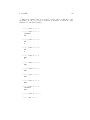
To obtain a history compatible with the spec, we perform:
(bezot:zot 10
(&& init the-lamp))
4
USAGE
24
This is an example history generated by Zot, where **LOOP**, and
**POOL** are the loop selector variables (**POOL** towards the past,
**LOOP** towards the future):
------ time 0 ----------- time 1 -----**LOOP**
ON
------ time 2 -----ON
L
------ time 3 -----ON
L
------ time 4 -----OFF
L
------ time 5 -----OFF
------ time 6 -----OFF
------ time 7 -----OFF
------ time 8 -----OFF
------ time 9 -----**POOL**
OFF
------ time 10 ----------- end ------
4
USAGE
4.6
25
Temporary data
Zot uses files to save temporary data during the verification activity. They
differ depending on the used plug-in. The propositional plug-in, like eezot,
creates
1) output.cnf.txt
2) output.sat.txt
3) output.hist.txt
(1) contains the resulting boolean formula of the system (in the standard DIMACS CNF format); (2) is the output of the SAT-solver; (3) is the
resulting trace of the system (e.g. a TRIO history), if it exists.
SMT-based ae2zot creates different files:
1)
2)
3)
4)
output.smt.txt
output.1.txt
output.hist.txt
output.dict.txt
(1) contains the resulting SMT-LIB description of the system (the standard is SMT-LIB v.1); (2) is the output of the SMT-solver, whose syntax
and structure vary with respect to the used solver; (3) is the resulting trace
of the system, if it exists. Finally, output.dict.txt is the set of all the subformulae which the tool handles
5
ARCHITECTURE
5
26
Architecture
Zot’s architecture is based on a PLTL-to-SAT core, which interacts with
the “outside world” through a TRIO-based interface and different plug-ins.
The core itself is structured as a plug-in, so that different encodings can be
defined and used.
More recently (May 2009), we added two plugins to Zot, natively supporting metric operators (like lasts, withinf). These native metric plugins
are called meezot (mono-infinite), and mbezot. Their usage is exactly the
same as eezot and bezot [17].
5.1
PLTL-to-SAT encodings
As said before, Zot’s core is based on encoding PLTL into SAT and CLTLB(IDL)
or CLTLB(LIA) into SMT. At present two main propositional encodings are
available in the standard distribution: eezot, which is a standard eventualitybased encoding on a mono-infinite time domain (N, see e.g. [8]), and the
bi-infinite one, bezot [18] on Z. The arithmetic encoding (see [6]) is implemented in ae2zot.
The two propositional encodings are packaged (as asdf systems) in the
following files:
eezot.lisp
bezot.lisp
eezot.asd
bezot.asd
The arithmetic encoding is packaged in:
ae2zot.lisp
ae2zot.asd
The file kripke.lisp contains the basic data structure and the definition
of the generics.4
(defclass kripke ()
(; time bound i.e. [0..k]
(the-k
:accessor kripke-k)
; number of used prop. variables
(numvar
:accessor kripke-numvar)
; formula -> integer data structure (hash-table)
(the-list
:accessor kripke-list)
; integer -> formula data structure (hash-table)
(the-back
:accessor kripke-back)
4
kripke does not actually contain a Kripke structure - names of data structures and
generics come from previous, forsaken incarnations of the tool-set.
5
ARCHITECTURE
27
; list of propositional letters
(sf-prop
:accessor kripke-prop)
; list of used boolean subformulae
(sf-bool
:accessor kripke-bool)
; list of used future-tense subf.
(sf-futr
:accessor kripke-futr)
; list of used past-tense subf.
(sf-past
:accessor kripke-past)
; n. of props used in the encoding
(max-prop
:accessor kripke-maximum)
; resulting SAT formula
(the-formula :accessor kripke-formula)))
There is also an old variant of eezot, called ezot, which supports virtual
unrollings (as presented in [8], usually called δ), so its data structure is
extended through inheritance. The user may change the default behavior
(i.e. δ = 0), by setting ezot:*FIXED-DELTA* to nil, which tells eezot to
actually compute δ, or (s)he may change to set it to a fixed meaningful
value.
The call generic translates a formula/proposition and a time instant into
an integer (the SAT-solver proposition); self must be an instance of kripke
(or of a subclass).
(defgeneric call (self obj the-time &rest other-stuff))
The back-call generic is used to translate an integer in [0..k] into the corresponding subformula; self must be an instance of kripke (or of a subclass).
(defgeneric back-call (self x))
(defgeneric back-call-time (self x))
5.2
Main Interface
There are two interfaces:
sat-interface.lisp
the first one is with the SAT/SMT-solver, and it is used to send the output
of the PLTL/CLTLB encoding to it; then, to parse its output and get a
counter-example, if any.
The other one,
5
ARCHITECTURE
28
trio-utils.lisp
is the basic interface with the user, and is based on TRIO (see Section 3.5)
augmented with the operational constructs covered in Section 3.6.
5
ARCHITECTURE
5.3
29
Other modules and plug-ins
At present just ap-zot and ta-zot are available. Please refer to Sections 3.7,
3.8, and the related papers.
The two plug-ins are implemented and packaged (as asdf systems) in
ap-zot.lisp
ta-zot.lisp
ap-zot.asd
ta-zot.asd
ta-zot is based on ap-zot, which uses TRIO as underlying language (through
the trio-utils interface).
Acknowledgments
I thank the following people: Stefano Riboni for his work on the CNF translator; Davide Casiraghi for the metric plugins (meezot and mbezot).
REFERENCES
30
References
[1] CVC3. http://http://www.cs.nyu.edu/acsys/cvc3/.
[2] Mathsat5. http://http://www.cs.nyu.edu/acsys/cvc3/.
[3] Microsoft Z3. http://z3.codeplex.com/.
[4] Smt library. http://smt-lib.org/.
[5] Yices2. http://yices.csl.sri.com/.
[6] M. M. Bersani, A. Frigeri, M. Pradella, M. Rossi, A. Morzenti, and
P. San Pietro. Bounded Reachability for Temporal Logic over Constraint System. In Proc. TIME, 2010.
[7] A. Biere. PicoSAT essentials. Journal on Satisfiability, Boolean Modeling and Computation (JSAT), 4:75–97, 2008.
[8] A. Biere, K. Heljanko, T. Junttila, T. Latvala, and V. Schuppan. Linear encodings of bounded LTL model checking. Logical Methods in
Computer Science, 2(5):1–64, 2006.
[9] N. E´en and N. S¨
orensson. An extensible SAT-solver. In SAT Conference, volume 2919 of LNCS, pages 502–518. Springer-Verlag, 2003.
[10] C. A. Furia, M. Pradella, and M. Rossi. Dense-time MTL verification through sampling. Technical Report 2007.37, DEI, Politecnico di
Milano, April 2007.
[11] C. A. Furia, M. Pradella, and M. Rossi. Dense-time MTL verification
through sampling. In Proceedings of FM’08, volume 5014 of LNCS,
2008.
[12] C. A. Furia, M. Pradella, and M. Rossi. Practical automated partial verification of multi-paradigm real-time models. Technical Report
arXiv.org 804.4383, April 2008.
[13] C. A. Furia, M. Pradella, and M. Rossi. Practical automated partial
verification of multi-paradigm real-time models. In 10th International
Conference on Formal Engineering Methods (ICFEM), October 2008.
[14] C. Ghezzi, D. Mandrioli, and A. Morzenti. TRIO: A logic language for
executable specifications of real-time systems. Journal of Systems and
Software, 12(2):107–123, 1990.
[15] M. Lewis, T. Schubert, and B. Becker. Multithreaded SAT solving. In
12th Asia and South Pacific Design Automation Conference, 2007.
REFERENCES
31
[16] M. W. Moskewicz, C. F. Madigan, Y. Zhao, L. Zhang, and S. Malik.
Chaff: engineering an efficient SAT solver. In DAC ’01: Proceedings of
the 38th Conf. on Design automation, pages 530–535, New York, NY,
USA, 2001. ACM Press.
[17] M. Pradella, A. Morzenti, and P. S. Pietro. A metric encoding for
bounded model checking. In A. Cavalcanti and D. Dams, editors,
FM 2009: Formal Methods, Second World Congress, Eindhoven, The
Netherlands, November 2-6, 2009. Proceedings, volume 5850 of Lecture
Notes in Computer Science, pages 741–756. Springer, 2009.
[18] M. Pradella, A. Morzenti, and P. San Pietro. The symmetry of the
past and of the future: Bi-infinite time in the verification of temporal
properties. In Proc. of The 6th joint meeting of the European Software
Engineering Conference and the ACM SIGSOFT Symposium on the
Foundations of Software Engineering ESEC/FSE, Dubrovnik, Croatia,
September 2007.
[19] M. Pradella, A. Morzenti, and P. San Pietro. Benchmarking modeland satisfiability-checking on bi-infinite time. In 5th International Colloquium on Theoretical Aspects of Computing (ICTAC 2008), Istanbul,
Turkey, September 2008.
[20] M. Pradella, A. Morzenti, and P. San Pietro. Refining real-time system specifications through bounded model- and satisfiability-checking.
In 23rd IEEE/ACM International Conference on Automated Software
Engineering (ASE 2008), L’Aquila, Italy, September 2008.