Download PIANOS user manual

PIANOS user manual
Group Linja
Helsinki 7th September 2005
Software Engineering Project
UNIVERSITY OF HELSINKI
Department of Computer Science
Course
581260 Software Engineering Project (6 cr)
Project Group
Joonas Kukkonen
Marja Hassinen
Eemil Lagerspetz
Client
Marko Salmenkivi
Project Masters
Juha Taina
Vesa Vainio (Instructor)
Homepage
http://www.cs.helsinki.fi/group/linja
i
Contents
1 Introduction
1.1
1
Version history . . . . . . . . . . . . . . . . . . . . . . . . . . . . . . .
1
2 Glossary
2
3 Installing PIANOS
4
4 Starting the program
4
5 Running the simulation
5
6 Input files
7
6.1
Model file . . . . . . . . . . . . . . . . . . . . . . . . . . . . . . . . . .
7
6.1.1
Names and constants . . . . . . . . . . . . . . . . . . . . . . . .
7
6.1.2
Defining global variables . . . . . . . . . . . . . . . . . . . . . .
7
6.1.3
Defining entities . . . . . . . . . . . . . . . . . . . . . . . . . .
10
6.1.4
Defining variables inside entities . . . . . . . . . . . . . . . . . .
11
6.1.5
Spatial operations . . . . . . . . . . . . . . . . . . . . . . . . . .
11
6.1.6
General restrictions . . . . . . . . . . . . . . . . . . . . . . . . .
13
6.1.7
Example model . . . . . . . . . . . . . . . . . . . . . . . . . . .
15
Simulation parameter files . . . . . . . . . . . . . . . . . . . . . . . . .
19
6.2.1
Simulation file . . . . . . . . . . . . . . . . . . . . . . . . . . .
19
6.2.2
Initial value file . . . . . . . . . . . . . . . . . . . . . . . . . . .
19
6.2.3
Proposal file . . . . . . . . . . . . . . . . . . . . . . . . . . . .
21
6.2.4
Update strategy file . . . . . . . . . . . . . . . . . . . . . . . . .
22
6.2.5
Parameters to output file . . . . . . . . . . . . . . . . . . . . . .
22
6.3
Data files . . . . . . . . . . . . . . . . . . . . . . . . . . . . . . . . . .
23
6.4
Adjacency matrix files . . . . . . . . . . . . . . . . . . . . . . . . . . .
24
6.5
User-defined distributions file . . . . . . . . . . . . . . . . . . . . . . . .
25
6.5.1
Definition lines . . . . . . . . . . . . . . . . . . . . . . . . . . .
25
6.5.2
Subroutines . . . . . . . . . . . . . . . . . . . . . . . . . . . . .
27
6.2
7 Outputs of the program
7.1
Outputs of the generator . . . . . . . . . . . . . . . . . . . . . . . . . .
29
29
ii
7.2
Outputs of the Fortran program . . . . . . . . . . . . . . . . . . . . . . .
8 References
29
30
1
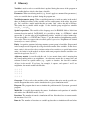
1 Introduction
This is the user manual of the PIANOS1 software. This software was produced on the
course “Software Engineering Project” of the department of Computer Science, University of Helsinki. PIANOS was implemented and designed by a group of research-oriented
students 2 .
This document describes the product, how to start it and the format of the input files.
The software product analyzes spatial data by using a semi-Bayesian model and prior
distributions to calculate points from the posterior distributions for a set of variables.
This kind of computation is heavy and time consuming on large sets of data. In order to
avoid creating one static program, which can run simulations with all possible models, the
program consists of two parts: the generator and the generated program. The generator
reads the input files and creates a customized Fortran program for the given problem.
The input files define the problem and how the program should run the simulation with
the given model. The main input file is the model file, which describes a semi-Bayesian
model. The model could describe, for example, a bird species’ distribution in Finland.
The main topic of interest is the question about the most accurate model to describe a
given real life phenomenon. The only way to compare the models is to compare the results. The program will not analyze how accurate the given model is, it will only calculate
points from the posterior distribution for variables and print them as output.
The program is limited to small set of possible simulation problems. There are limitations
to the models and distributions that can be used. The key feature is the possibility to use
spatial relations in the calculations.
The generator can be executed on any computer with the Java runtime environment version 1.5 (or greater) installed. The generated program however needs a Fortran 90 compiler. It also uses NAG libraries, so a computer with a valid NAG license is required. The
program was designed with NAG Mark 19.
1.1 Version history
Version
0.2
1.0
1.1
1
2
Date
29.07.2005
22.08.2005
25.08.2005
Modifications
Document template
First full-featured draft
Reviewed and corrected final
Probabilistic Inference ANd Other Stuff
http://www.cs.helsinki.fi/opiskelu/tutkijalinja/ at the department
2
2 Glossary
Variable is used to refer to a variable that is updated during the course of the program or
to a variable that has a fixed value from a data file.
Parameter: When considering models (e.g. doesn’t apply to command-line parameters),
refers to a variable that is updated during the program run.
Variable/parameter group: When a variable/parameter is inside an entity in the model,
there are multiple instances of the variable; one for each instance of the entity. An example: Let’s consider a model model that has an entity ‘bird’ with a data file of 50 lines.
This entity has a variable called weight. So the variable group weight has variables
weight1 , ..., weight50 .
Spatial expressions: The models of the language used in PIANOS differ a little from
common bayesian models. In PIANOS, it is possible to define ‘a = SUM(&x)’ which
means that ‘a’ gets the value of all neighbouring entities’ variable x’s values summed up.
We can also define ‘a = COUNT(&x)’ where ‘a’ gets the number of neighbouring entities
as its value. These two expressions are called spatial expressions. Neighbours are defined
in an adjacency matrix (below).
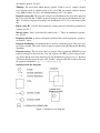
Entity: A repetitive structure (indexing structure, parent group) of variables. Represented
in the example model diagrams by a large box that contains some variables. In this document, entity is also used to refer to an intersection of two entities as a special intersection
entity. An entity is in the models an object with some properties that the variables contained in it represent. See 6.1.3
Adjacency matrix: A text file with 0:s and 1:s in a matrix form, each 1 meaning that
the corresponding indices are neighbours. An adjacency matrix has as many lines and
columns as there are spatial entities (e.g. squares or counties, the data file’s number
of lines) in the model. If we have, for example, 4 squares, and squares 1 and 3 are
neighbours, the matrix would look like this:
0
0
1
0
0
0
0
0
1
0
0
0
0
0
0
0
Generator: Used to refer to the modules of the software that write out the specific executable Program that carries out the simulation for a given simulation model.
Program: The program that is run to simulate the problem model. Synonym: generated
program.
Model file: A text file that contains the names, distributions and equations of variables
and entities for a PIANOS model. See 6.1
Iterations: The number of rounds a simulation will last. Note that burn-in counts towards
the iterations. See 6.2.4
Burn-in: The number of iterations or variable updates that a simulation will run before
3
any output is printed. See 6.2.1
Thinning: The period after which output is printed. If this is set to 1, output is printed
every iteration round or variable update, if it is set to 100, for example, output is printed
every 100th iteration. See 6.2.1 for defining thinning, and 7.2 for output.
Proposal strategy file: The proposal strategies and distributions file (also called proposal
file) is used for just that: it defines proposal strategies and proposal distributions for variables. See below for proposal strategies and distributions, See 6.2.3 for the format of the
file.
Initial values file: a text file that contains the starting values for simulated parameters in
a model. See 6.2.2
Missing values: ‘holes’ in the data file, marked with ‘*’. These are simulated as parameters. See 6.3
Frequency function: A density or frequency function that is used to gauge the ‘goodness’
of variables’ values.
Proposal distribution: A distribution that is used for calculating a new value to be proposed for a variable. This value is then accepted or rejected using the Metropolis-Hastings
algorithm.
Proposal strategy: The way new values are proposed for a parameter. PIANOS has two
proposal strategies to choose from: fixed and random walk (RW). A fixed proposal strategy means that the new value from the proposal distribution is proposed ‘as is’. Random
walk means that the proposed value is the variable’s current value added to the value from
the proposal distribution, e.g. x0 = x + unif orm(−1, 1)
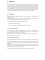
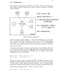
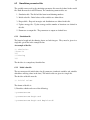
Symbols used in the diagrams:
Figure 1: Symbols used in diagrams.
4
3 Installing PIANOS
There is no installing to be done with PIANOS. The program is path-independent and
runnable right from the CD-ROM (it cannot write the generated program on the CDROM, though). The only thing that needs to be done is to pick a directory and copy
everything from the directory ‘release’ (on the CD-ROM) there. After doing this you are
ready to run PIANOS.
Note that PIANOS requires a Java runtime environment of version 1.5 or later.
4 Starting the program
This section describes how to run PIANOS and also acts as a quick-start guide. There are
several example models and simulation files that can be used for experimentation in the
directory ‘release/models’ on the PIANOS CD-ROM or the tar.gz package. The directory
release also contains examples on how to run PIANOS.
There are two methods to run PIANOS on the command-line, and one Java static method
for further development.
On the command-line, the user can specify one file that contains the file names of the
simulation parameter files and the model file, or these files can be given directly on the
command-line.
An example:
java -jar PIANOS.jar allfiles.txt
In this case, ‘allfiles.txt’ should contain file names in the format:
user distributions:
model:
initial values:
simulation:
proposals:
update strategy:
to output:
last values:
relative/path/to/user_dist.f90
relative/path/to/modelFile
relative/path/to/initialValuesFile
relative/path/to/simulationFile
relative/path/to/proposalsFile
relative/path/to/updateFile
relative/path/to/toOutputFile
relative/path/to/lastValuesFile
Here the order of the header - file name pairs is arbitrary. this file can also contain empty
lines and comment lines (starting with a hash ‘#’).
Note that the file name of the user distributions file must always be ‘user_dist.f90’ and it
must contain a valid Fortran module named ‘user_dist’ (even when all used distributions
would be provided ones).
The other method on the command line is used like this:
5
java -jar PIANOS.jar user_dist.f90 modelFile initialValuesFile
simulationFile proposalsFile updateFile
toOutputFile lastValuesFile
Here each parameter is the relative path to the file such as above.
As the user can see, the methods differ only in the way of providing the necessary files.
Refer to the Javadoc documentation for details on the Java method to run PIANOS with.
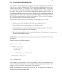
5 Running the simulation
After PIANOS has finished there should be a couple of .f90-files in the program directory.
These are the simulation program that can be compiled and run on a computer with a
Fortran compiler and the NAG library. List of produced files:
• definitions.f90
• input.f90
• main.f90
• output.f90
• proposal.f90
In addition to these the user needs a Fortran module file named ‘user_dist.f90’ that contains the user-defined distributions for the model used. With PIANOS are provided a
few of these, one for each example model and one that combines all the contents of the
separate files for the models. The larger collection of distributions can be found in the
directory ‘release/models’ while each model’s specific user_dist.f90 can be found in the
model’s directory ( ‘release/models/themodel’).
The simulation program requires some of the model files, including data and initial values
file, to be available when it is started. To be on the safe side, we encourage users to copy
all of the model files to the computer used for the simulation.
Note that the files need to be in the same relative path as they were when running the
PIANOS generator program.
An example:
We have PIANOS at ‘home/we/PIANOS/release’. We have the model files for the example model called simplebirds_spatial in ‘home/we/PIANOS/release/models/simplebirds_spatial’.
First we run PIANOS:
java -jar PIANOS.jar models/simplebirds_spatial/allfiles.txt
6
Now, we transfer the .f90-files to a suitable computer:
scp *.f90 models/simplebirds_spatial/user_dist.f90
we@computer:work/.
We already have a directory called models under ‘work/’ at the computer. We transfer the
model files there:
scp -r models/simplebirds_spatial/
we@computer:work/models/.
Now we only need to compile and run the simulation at the computer.
When all these files are on a suitable computer, compiling and running the simulation is
done like this:
f95
f95
f95
f95
f95
-lnag
-lnag
-lnag
-lnag
-lnag
-c
-c
-c
-c
-c
definitions.f90
proposal.f90
user_dist.f90
input.f90
output.f90
f95 -lnag -o main main.f90 definitions.o
proposal.o user_dist.o input.o output.o
./main
Note that running a simulation with a large number of iterations might take a long time.
The simulation prints messages on its progress while it is running. See 7.2 on the outputs
of the simulation.
7
6 Input files
This section describes the input files. The generator reads the input files and generates a
program for the given problem. Should the user change any input files after running the
generator, he/she needs to run the generator again before the changes are reflected to the
generated program. The generated program writes a summary of all the variables at the
end of a simulation run (see 7.2). It’s possible to continue the simulation later with these
values as data and/or as initial values. However it is the user’s responsibility to copy those
values to the initial value and data files and adjust the model file accordingly.
6.1 Model file
The model file describes the Bayesian model used in the simulation. The file must be in
ASCII text format.
A model description consists of variable and entity definitions. It can also include comment lines, any line beginning with ‘#’ is considered a comment.
The model description file consists of the following parts:
1. Definitions of global variables
2. Definitions of entities, which contain definitions of variables
6.1.1 Names and constants
Names of variables and entities can include lowercase letters ‘a’ - ‘z’ and numbers ‘0’ ‘9’. A name must start with a letter. No other characters are allowed. The variable names
must not be equal to any reserved words of Fortran.
Floating point constants may be expressed using the scientific format except that the exponent ‘E’ must be an uppercase ‘E’.
6.1.2 Defining global variables
Variables can be either integer or floating point type. Every variable is also either stochastic or functional. Stochastic variables can also be data variables, if they are defined inside
an entity. Global variables can be stochastic or functional, but they can not be defined in
a data file.
NOTE: Variables must be defined in topological order; That is, if the variable ‘alpha’
affects variable ‘beta’ then alpha must be defined before beta. Functional variables with
spatial expressions are an exception, see 6.1.5.
The definition of global variables should be before any definition of an entity.
8
NOTE: Chaining of multiple functional variables is not allowed! The chain of two functional variables can be expressed by one functional variable. Functional variables with
spatial expressions are an exception, more about this later.
The type of a variable is expressed by an ‘INTEGER’ or ‘REAL’ in front of their names.
The syntax is:
type name ...
type name ...
For example:
REAL alpha ...
INTEGER delta ...
If the variable is functional, an equation must be provided. If the variable is stochastic, a
distribution must be provided (variables coming from data are an exception). The syntax
is:
type name ~ distribution
type name = expression
For example:
REAL alpha = 1 * gamma
INTEGER delta ~ poisson(alpha)
Distributions
The following distributions are possible for INTEGER variables:
• discrete_uniform(INTEGER a, INTEGER b)
• binomial(INTEGER n, REAL p)
• poisson(REAL mu)
• user_bernoulli(REAL p)
The following distributions are possible for REAL variables:
• continuous_uniform(REAL a, REAL b)
• beta(REAL alpha, REAL beta)
• user_gamma(REAL a, REAL b)
9
• user_normal(REAL mu, REAL sigma2)
Note that it’s possible to define other “user-defined” distributions. The name of these
distributions must start with ‘user_’. The user defined function file is described in 6.5.
Examples:
REAL alpha ~ beta(0.1, 1.0)
INTEGER delta ~ poisson(alpha)
Expressions
Expressions are not allowed as parameters for distributions. A parameter must be a real
or integer number, depending on the type of the distribution, or a variable of the correct
type.
List of operators allowed in equations
The following operations are possible:
• +
• • *
• /
• ** (power expression in Fortran)
• EXP()
• LOG()
• Fortran intrinsic functions (such as SIN())
• Type conversions (such as REAL())
Examples:
REAL beta = alpha**2
REAL gamma = EXP(alpha + 1) / EXP(alpha - 1)
There are two spatial operations SUM() and COUNT(). See 6.1.5.
The user must take care of type conversions, that is, the program doesn’t perform any type
conversions other than the conversions automatically performed by Fortran.
Examples:
INTEGER n = ...
INTEGER p = ...
REAL q = REAL(p) / n
10
6.1.3 Defining entities
An entity is an object that groups variables together. An entity can describe for example
a bird species or a geographical area.
The first line, identified with ENTITY, defines the name of the entity. It also defines the
data file where all data about the entity is found (if some variables from the entity are
taken from data), the data file name defining spatial relations (if it exists) and which other
entities the entity combines (if the entity describes an intersection of two entities).
The adjacency matrix which defines spatial relations is defined in 6.4. The format of data
files is defined in 6.3.
Examples:
ENTITY bird, "birds.txt"
{
...
}
In this example the name of the entity is ‘bird’ and the data file is ‘birds.txt’.
If no data is provided, the data file name must equal “”. It is also possible that an entity
has no variables in it. For example:
ENTITY bird, ""
{
}
ENTITY square, "squares.txt", "spatial.txt"
{
...
}
Similarly we define an entity called square. In this example, ‘square’ is a spatial unit, so
a file name of the adjacency matrix is given.
ENTITY observation, "observations.txt", combines(square, bird)
{
...
}
This example shows how to define an intersection entity. The combines-clause states that
the squares are the vertical units and birds are the horizontal units in the matrices related
to the intersection entity (for example, data matrices).
NOTE: an intersection entity cannot be spatial. Also, a model file may define only one
spatial entity.
11
6.1.4 Defining variables inside entities
The variables related to the entity are defined inside the brackets. The variables inside
entities can be defined in a data file. This is done by adding “(column_number)” after
the variable name, where column_number defines the column of the data file in which the
corresponding data is found. If the data is a matrix, there is no single column containing
the data and this situation is specified simply by adding “(*)” after the variable name.
The variables are defined in the same way inside entities, as are the global variables.
Examples:
ENTITY bird, "birds.txt"
{
REAL size(1)
}
ENTITY square, "squares.txt", "spatial.txt"
{
INTEGER northerness(1)
}
ENTITY observation, "observations.txt", combines(square, bird)
{
REAL p = EXP(alpha * northerness) / (1 + EXP(alpha * northerness))
INTEGER x ~ user_bernoulli(p)
INTEGER obs(*) ~ user_defined_points(x)
}
6.1.5 Spatial operations
Functional parameters describing spatial relations can be defined inside entities, which
have an adjacency matrix defined. Spatial functional parameters can also be used inside
an entity which combines a spatial and a ‘normal’ entity.the character ‘&’ has a special
meaning ‘all neighbouring units’. & x means ‘all instances of the variable x in neighbouring units’.
The referenced variable in a &-expression can only be a stochastic variable. For example,
in ’& x’ the variable x must be stochastic.
The following spatial operations are possible:
• SUM(&variable)
• COUNT(&variable)
A functional variable can only have one spatial operation in it. (e.g. One cannot define ‘a
= SUM(&x) * 53’ or ‘a = SUM(&x)/COUNT(&x)’) (see 6.1.6)
12
Example:
ENTITY square, "squares.txt", "spatial.txt"
{
INTEGER n = COUNT(&mu)
REAL p = SUM(&mu)
REAL alpha = p / n
REAL mu ~ beta(alpha, beta)
}
In this example alpha is the average of all neighbour mu variables. Since we need to
define variable in topological order, alpha needs to be defined before mu. Also p and n
must be defined before alpha. However as you can see topological order is not possible
with spatial variables since n and p depend on mu, which is defined after them. In cases
like this the functional variables with a SUM() or COUNT() operation can and must be
defined before the variable they depend on.
There is also a chain of functional variables in the last example. Chaining functional variables is only allowed in spatial cases like this, since SUM() and COUNT() must appear
in separate variables’ expressions.
13
6.1.6 General restrictions
There are a few global restrictions to the semantics of the model description file.
Spatial operations A functional variable can have a SUM() or COUNT() operation in its
expression. If either of these operations is used, no other operations may be used in the
expression.
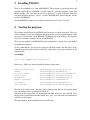
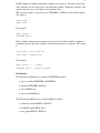
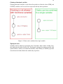
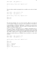
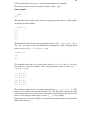
Dependencies between variables
A global variable can affect another global variable, a variable inside an entity or a variable inside an intersection of entities.
A variable inside an entity can affect a variable inside the same entity, or a variable inside
an intersection of entities where either one is the entity of the affecting variable.
A variable inside an intersection of two entities can only affect a variable inside the same
intersection.
Cycles are not allowed in the model, excluding the spatial relations.
Figure 2: Allowed dependencies
14
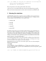
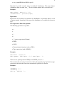
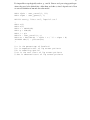
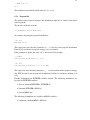
Chaining of functional variables
Chaining functional variables is only allowed in spatial cases like this, where SUM() and
COUNT() variables can’t be used in an expression with any other operations.
Figure 3: Chains can be combined into single variable.
Topological order
Variables must be defined in topological order. If variable ‘alpha’ affects variable ‘beta’
then alpha must be defined before beta. Topological ordering is not always possible with
spatial variables. In these cases functional variables, with a SUM() or COUNT() operation
can and must be defined before the variable they depend on.
15
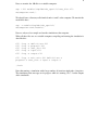
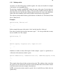
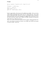
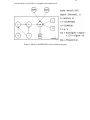
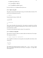
6.1.7 Example model
In this section we will construct a model file from scratch. We will use the lip cancer
model, which describes the amount of lip cancers among the populations of different
regions in England.
Figure 4: Model in logical form.
‘alpha’ and ‘sigma’ are global variables. ‘e’ is the expected number of cases in a county
and ‘x’ describes the amount of farmland in a county. ‘mu’ is a variable which combines
other variables. ‘b’ contains a spatial expression. Note that ‘b’ is not valid PIANOS
model format. The spatial operations need to be split into their own variables. We will do
this later in this section.
As the figure shows, alpha and sigma are global variables. They should be defined first
since they do not depend on any other variable. The normal and gamma distribution have
been programmed in the testing phase of PIANOS. they are examples of user-defined
distributions and are used in this model.
REAL alpha ~ user_normal(0, 100)
REAL sigma ~ user_gamma(1, 1)
The figure has only one entity. It is spatial (COUNT() and SUM() operations are used)
and there are variables which are defined in data (obs, x and e). Let’s assume the data file
is called ‘data.txt’ and the adjacency matrix file ‘spatial.txt’. Let’s also assume that the
variable obs is defined in the first column, x in the second and e in the third column. The
entity describes a geographical area, a county, so lets call it ‘county’.
REAL alpha ~ user_normal(0, 100)
16
REAL sigma ~ user_gamma(1, 1)
ENTITY county, "data.txt", "spatial.txt"
{
...
}
We need to define variables in topological order, so variables x and e need to be defined
next.
REAL alpha ~ user_normal(0, 100)
REAL sigma ~ user_gamma(1, 1)
ENTITY county, "data.txt", "spatial.txt"
{
REAL x(2)
REAL e(3)
...
}
We assume here that both x and e are real type in the data. Before we can define mu
we need to define b. However as you can see, we hit a problem here. B is defined as
b ñormal(SUM(&b) / COUNT(&b), COUNT(&b)). A distribution can only have fixed
numbers or variables as parameters. We need to replace the operations with two new
variables. Lets call those variables ‘t and ‘n’.
Now we can define n as n = COUNT(&b) and t as t = SUM(&b) / COUNT(&b). However
we still have a problem. T has three operations in it’s expression. Since we are using
spatial operations, only one is allowed. We need to replace both spatial operations with
new variables. Luckily we have a variable for COUNT() already, the variable n. Lets
define a new variable called q as q = SUM(&b). Now we can define b, n, t and q in the
model file:
REAL alpha ~ user_normal(0, 100)
REAL sigma ~ user_gamma(1, 1)
ENTITY county, "data.txt", "spatial.txt"
{
REAL x(2)
REAL e(3)
REAL n = COUNT(&b)
REAL q = SUM(&b)
REAL t = q/n
REAL b ~ user_normal(t, n)
...
}
17
It’s impossible to topologically order n, q, t and b. Since n and q are using spatial operations, they need to be defined first. After them we define t, since b depends on it. Now
we can add definition of mu and obs to the model.
REAL alpha ~ user_normal(0, 100)
REAL sigma ~ user_gamma(1, 1)
ENTITY county, "data.txt", "spatial.txt"
{
REAL x(2)
REAL e(3)
REAL n = COUNT(&b)
REAL q = SUM(&b)
REAL t = q/n
REAL b ~ user_normal(t, n)
REAL mu = EXP(LOG(e) + alpha * x / 10 + sigma * b)
INTEGER obs(1) ~ poisson(mu)
}
#
#
#
#
#
x is the percentage of farmland
e is expected count of lip cancer patients
b is something spatial
mu is the real count of lip cancer patients
obs is observed count of lip cancer patients
18
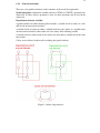
Our model file is ready. Here is a graphical presentation of it.
Figure 5: Model in the PIANOS model description language.
19
6.2 Simulation parameter files
The variable names used in the simulation parameter files must be defined in the model
file. Each file must be in ASCII format. The simulation parameter files are:
1. Simulation file - The file hold the burn-in and thinning numbers.
2. Initial value file - Initial values of the variables are defined here.
3. Proposal file - Proposal strategies and distributions are defined in this file.
4. Update strategy file - Update strategy and the number of iterations are defined in
this file.
5. Parameters to output file - The parameters to output are defined here.
6.2.1 Simulation file
The burn-in length and the thinning factor are both integers. They must be given in a
single file, given like in the example below:
An example of the file:
?? simulation
? burn-in
100
? thinning
100
The first line is a compulsory identifier line.
6.2.2 Initial value file
The user must provide initial values for all parameters (stochastic variables and variables
which have missing values in the data). The initial values are given in a single file.
The first line of the file must be:
?? initial values
The format of the file is:
1) Identifier, which can be one of the following:
? parametername
? parametername begin:end
? parametername begin:end begin2:end2
20
2) The initial values in an array or a matrix corresponding to the identifier.
The file may contain several consecutive identifier - values - pairs.
Some examples:
? alpha
4.0
The identifier of the example means that we are giving an initial value to a single variable
on the line after the identifier.
? alpha 1:5
3.2
0.3
3.1
5.3
2.9
The identifier describes that we are giving initial values to alpha1 , alpha2 , alpha3 , alpha4
and alpha5 in an array on the lines following the identifier line. After setting the initial
values, we have alpha1 = 3.2, alpha2 = 0.3 etc.
? beta 1:3
5.4
2.1
1.0
The identifier means that we are giving initial values to beta1 , beta2 and beta3 in an array on the lines after the identifier. After setting the initial values, we have beta 1 =
5.4, beta2 = 2.1 etc.
? x
1.0
1.2
3.8
4.4
5.6
1:5
3.2
5.2
4.1
2.7
0.4
1:3
5.3
3.1
8.0
3.2
1.2
The identifier describes that we are giving initial values to x1,1 , x1,2 , x1,3 , x2,1 , ...x5,3 . The
values are in a matrix form after the identifier line. The first index corresponds to the
vertical dimension and the second index corresponds to the horizontal dimension of the
matrix. After setting the initial values, we have x3,2 = 4.1 for example.
If some instances of, say, the variable obs are missing from the data, the user must provide
initial values for them.
21
? obs 4:4 1:1
4.3
This definition states that the initial value of obs4,1 is 4.3.
6.2.3 Proposal file
The format of the proposal strategies and distributions input file is similar to the initial
values input file.
The first line of the file must be:
?? proposal distributions
An example of giving the proposal distributions:
? b all
poisson(3.0)
This expression states that the parameters b1 , ..., b5 have the same proposal distribution
Poisson(3.0) and the fixed proposal strategy is used as default.
If the parameter is global, the word “all” is not needed. For example:
? alpha
continuous_uniform(0.0, 2.0)
? b all
continuous_uniform(-1.0, 1.0) RW
This expression states that the parameters b1,1 , ... use the random walk as proposal strategy
(the ‘RW’ keyword) and the proposal distribution for them is continuous_uniform(-1.0,
1.0).
Possible distributions for INTEGER variables include: The following distributions are
possible for INTEGER variables:
• discrete_uniform(INTEGER a, INTEGER b)
• binomial(INTEGER n, REAL p)
• poisson(REAL mu)
The following distributions are possible for REAL variables:
• continuous_uniform(REAL a, REAL b)
22
• beta(REAL alpha, REAL beta)
• user_gamma(REAL a, REAL b)
• user_normal(REAL mu, REAL sigma2)
It is also possible to use a distribution defined by the user.
6.2.4 Update strategy file
The update strategy file defined the update strategy used and the number of iterations. The
first line of the specification file must be:
?? update
Sequential update strategy is defined with:
? strategy
sequential
? iterations
42
The user gives the number of iterations, that is: the parameters are updated once and then
the output is printed (considering the thinning factor of course) and this is repeated until
the iteration count is reached.
Currently the only implemented update strategy is the sequential one.
6.2.5 Parameters to output file
The parameters to output are defined in a manner similar to the initial values. For example:
The compulsory identifier is:
?? output outputFile summaryFile
where outputFile is the filename of the output file and summaryFile is the filename of the
summary file.
? b all
? mu all
? alpha
This definition states that the parameter to output are all b : s, all mu : s and alpha. Note
that it is not possible to define that only some instances, for example b 1 , are output. More
about outputs in 7.2
23
6.3 Data files
Data files can be in a column or matrix format. A data file needs to be defined for each
entity that contains a variable getting its values from data.
Data files must be saved in ASCII format. All the rows (and columns) of a data file should
be of equal length (e.g. no blank positions or uneven lines allowed). Accepted values are
integers, real numbers and the missing value sign (*). Values are separated with a space
on the rows. Comments are allowed in data files. The comment sign is ‘#’. Empty lines
are allowed in data files.
Missing values are denoted by ‘*’. Should a variable have missing values in its data, the
variable needs a proposal distribution and initial values for missing data. Initial values
and proposal distributions are defined in the simulation parameter files. The program
considers missing values as parameters and proposes new values to them.
Should the entity’s variables be in “column format”, that is no “combines” word in the
entity definition, then the data file has to be in column format. In column format each
column defines one variable’s values. It’s possible for a data file in the format to contain
more columns than actual variables which are defined in the model file. In this format, all
the values in a column must be in the same format: integer or real. Note that in the real
format the number ‘1’ must be written as ‘1.0’.
If the entity combines two other entities, the variables defined inside the entity are in
matrix format. In matrix format, the size of the data file is fixed by those two entities’
data files, which the current entity combines.
Example:
ENTITY observation, "observations.txt", combines(square, bird)
{
...
}
Now the observation.txt must be in matrix format. The file must have as many rows as
square entity’s data file has and as many columns as bird entity’s data file has rows. The
data files also needs to be in either integer or real format.
24
6.4 Adjacency matrix files
Spatial dependencies are defined in an adjacency matrix file. An adjacency matrix file
can only be defined to a single one dimension entity (no combines word in its definition).
The entity’s data file defines the size of the adjacency matrix. The number of rows and
columns must be exactly the same in the adjacency matrix as is the number of rows in the
entity’s data file (excluding comments). Adjacency matrix files must be saved in ASCII
format.
Each row (or column) in the adjacency matrix defines the neighbours of a variable. Position (i, j) defines if the i:th and j:th variables are adjacent. Value ‘0’ means that the
variables are not adjacent or neighbours and value 1 means they are.
Example:
A
8
7
1
4
data file:
2 3
9 2
6 7
8 9
An adjacency matrix file:
0 1 0 0
1 0 0 0
0 0 0 1
0 0 1 0
Let’s assume that variable alpha is defined on the 1st column of the data file. Now actually
the alpha group has 4 variables since we have 4 rows in the data file. The variables are
alpha_1 = 8, alpha_2 = 7, alpha_3 = 1, and alpha_4 = 4.
In our example, variable alpha_1’s neighbour is alpha_2 (and alpha_2’s neighbour is
alpha_1). Alpha_3’s neighbour is alpha_4.
25
6.5 User-defined distributions file
It is possible to add distributions to the program. These new distributions are defined and
found in a user-defined distribution file. The program takes the filename of the file as a
command line parameter. It’s possible to use a unique distribution file in every model,
or to use only one user-defined distribution file. The file must be a Fortran 90 source
file named ‘user_dist.f90’. It must contain a valid Fortran module named ‘user_dist’. A
user-defined distribution consists of two parts. The first one is an introductory line at the
beginning of the file and the second part are the Fortran subroutines and functions in the
file. One file can hold multiple user-defined distributions. The user-defined distribution
file is compiled with the rest of the Fortran modules.
When the user wants to add an own distribution, the following steps are needed:
1. Decide a name for the distribution. The name must begin with ‘user_’.
2. Add a definition line in the beginning of user-distribution file.
3. Add a subroutine user_name_freq() into the user-distribution module. The parameters depend on the parameters of the distribution.
4. If the distribution could be used as a proposal distribution, add a subroutine user_name_gen()
into the user-distribution module.
NOTE: Both user_name_gen() and user_name_freq() need to be subroutines. They cannot
be functions.
The file needs to be in following format:
Definition lines
MODULE user_dist
IMPLICIT NONE
CONTAINS
Subroutines and functions
END MODULE user_dist
6.5.1 Definition lines
The program reads the definition lines at the beginning of the user-distribution file and
creates a distribution objects into its data structures. The program assumes that the subroutines are present and in the same format as the definitions.
NOTE: The definitions need to be at the start of the file. No empty lines, comments, or
any other lines are allowed before them.
26
Since the module is compiled, the definitions need to start with Fortran comment mark ‘!’.
Should you want to add Fortran comments to the beginning of the module, add an empty
line after the last definition and begin the comment from the next line after the empty line.
The definition line has the following syntax:
! name param_count types gen_present
Where
• name is the name of the distribution
• ‘param_count’ is the number of distribution’s parameters
• ‘types’ contain as many types as param_count suggests
• each type is either INTEGER or REAL
• gen_present is .TRUE. if there is a subroutine that generates proposals from the
distribution, .FALSE. otherwise.
NOTE: ‘param_count’ is the number of the distribution’s parameters, not the number of
the subroutine’s parameters.
The name of the distribution needs to start with ‘user_’. For example a valid name would
be ‘user_gamma’. This function could then be used in the model and proposal distribution
file with the name ‘user_gamma’.
The parameters count is the amount of the parameters of the distribution. For example for
the Normal distribution the count would be two, for the Poisson distribution it would be
one. Note that the program assumes that a generation subroutine has one more parameter
than the ‘param_count’ and that the frequency function has two more parameters. These
extra parameters are the point for which the frequency is calculated and the return value
parameter.
‘types’ is a list of parameter types. Should the parameter count be two for the distribution,
you need to define the types of both.
The last field ‘gen_present’ tells if distribution has a generation function defined in the file.
The generation function is required for generating proposals from the distribution. It is
optional (the distribution can be used for variables that are not updated) but the frequency
function is always required.
An example:
! user_points 1 INTEGER .FALSE.
This distribution could be used with the name ‘user_points’ in the input files. It has only
one parameter which is an integer type. It does not have a generation function, so it can
not be used as a proposal distribution. It could be used in the model file in this manner:
An example:
27
INTEGER alpha ...
INTEGER beta ~ user_points(alpha)
NOTE: The return value isn’t defined. It’s up to the user to use correct distributions for
integer and real variables.
6.5.2 Subroutines
The parameters of user_name_freq and user_name_gen subroutines depend on the parameters of the distribution: the subroutine implementing the frequency function has two
additional parameters (the point on which the frequency is calculated and the result) and
the subroutine generating the proposals has one additional parameter (the array which to
generate proposals to).
Should a distribution be defined as ‘! user_normal 2 REAL REAL .TRUE.’ in the beginning of the file, the frequency and generation functions need to be in following format:
SUBROUTINE user_normal_freq(param1, param2, point, result)
! param1 and param2 are real type
...
END SUBROUTINE user_normal_freq
SUBROUTINE user_normal_gen(param1, param2, result)
! param1 and param2 are real type
...
END SUBROUTINE user_normal_gen
NOTE: The generation subroutine is assumed to generate an array full of proposals.
NOTE: All user-defined subroutines and functions that user REAL variables must define
them as REAL (KIND=SELECTED_REAL_KIND(8,0)) for compliance with NAG.
NOTE: It is possible to program the subroutines to use existing NAG subroutines.
NOTE: You can add other functions and subroutines to the file and use them in the required subroutines.
An example:
! user_gamma 2 REAL REAL .TRUE.
MODULE user_dist
IMPLICIT NONE
CONTAINS
SUBROUTINE user_gamma_freq(alpha, lambda, point, freq)
28
...
END SUBROUTINE user_gamma_freq
SUBROUTINE user_gamma_gen(param1, param2, buffer)
...
END SUBROUTINE user_gamma_gen
END MODULE user_dist
29
7 Outputs of the program
This section outlines the outputs of PIANOS, that is, the generated Fortran program and
its outputs.
7.1 Outputs of the generator
The generator outputs Fortran source code into Fortran module files. These files are:
• definitions.f90, the file containing the Fortran data structures necessary for the simulation
• proposal.f90, the module that handles proposing new values for variables
• input.f90, the module that handles reading of data into the Fortran program
• output.f90, the module that writes out results of the simulation
• main.f90, the main program, uses other modules and runs the simulation
The generator also produces a modified data file and a binary map of missing values for
each data file, named datafile_1.txt and datafile_missing.txt (naming may vary). These
must be in the same relative path that the data files are defined in the model file for the Fortran program. In addition to these, running of the result program requires user_dist.f90,
a Fortran module file that contains the user-defined distributions necessary for the model
(or an empty module if none are necessary). This should be in the same directory with
the other modules.
7.2 Outputs of the Fortran program
The Fortran program, once compiled and run, produces three files. The last values file that
contains the last values at the end of the simulation (replace the initial values file with this
to continue the simulation with these), the update summary file that details the number of
updates proposed for each variable that has been chosen to output and a ratio of accepted
updates, and update values that contains the values of variables chosen to output for each
round of updates not thinned out. Note that the names of the update summary and update
values files must be given in the parameters to output file (See 6.2.5). The name of the
last values file is given when starting the program (See 4)
30
8 References
jdoc PIANOS javadoc documentation
http://www.cs.helsinki.fi/group/linja/PIANOScdrom/src/java/doc/