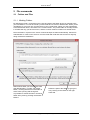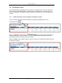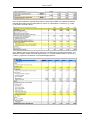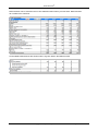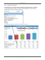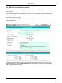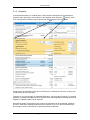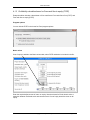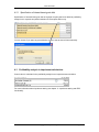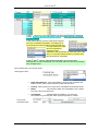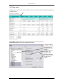
1
Invest for Excel® Version 3.7 Earnings and FCF 3 000 000 60% 58% 2 500 000 56% EUR 2 000 000 54% 1 500 000 52% 50% 1 000 000 48% 500 000 46% 0 44% 12/2016 Turnover 12/2017 12/2018 EBITDA 12/2019 12/2020 12/2021 12/2022 Free cash flow to firm (FCFF) User Manual Copyright © Datapartner Oy 12/2023 12/2024 EBITDA margin % for Excel Page 2 Copyright © Datapartner Oy 11/17/2014 Invest for Excel® Copyright DataPartner Oy DataPartner Oy accepts no responsibility for any errors or omissions in this publication. Furthermore, DataPartner Oy accepts no liability for damages arising from the use of the program or this manual. All rights are reserved regarding copying, distribution and translation of this document. This program is covered by copyright legislation. Unauthorised duplication and distribution of the program or its contents is prohibited. Any copying of the program apart from a safety copy for personal use is prohibited. DataPartner Oy is not responsible for a program package tampered or altered in any way by the purchaser or a third party. Microsoft Excel, Office and Windows are registered trademarks of Microsoft Corporation. Acrobat Reader is a registered trademark of Adobe Systems Incorporated. The supplier accepts no liability for any indirect loss or damage suffered by the customer due to supplier’s delay or omission. Therefore, the supplier is not responsible for the correctness of calculations and cannot be held liable for any economic consequences of decisions made on the basis of the calculations. The supplier’s liability for damages will under no circumstances exceed the price paid for the program. DataPartner Oy Raatihuoneenkatu 8 A FIN-06100 Porvoo Tel. +358-19-54 10 100 Fax: +358-19-54 10 111 E-mail: [email protected] [email protected] Internet: http://www.investforexcel.com 11/17/2014 Copyright © Datapartner Oy Page 3 Invest for Excel® Page 4 Copyright © Datapartner Oy 11/17/2014 Invest for Excel® Table of contents 1 INTRODUCTION ............................................................................................................................. 10 1.1 SYSTEM REQUIREMENTS ............................................................................................................... 10 1.2 INSTALLATION .............................................................................................................................. 10 1.3 SOLVING PROBLEMS ..................................................................................................................... 12 1.4 START-UP ..................................................................................................................................... 12 1.5 COMPONENTS ............................................................................................................................... 14 1.6 ENTERING DATA .......................................................................................................................... 14 1.7 WORKING ORDER ......................................................................................................................... 15 1.8 HOME SCREEN (START-UP SCREEN) ............................................................................................. 16 1.9 GENERAL BUTTONS ...................................................................................................................... 18 1.9.1 Picture copy ......................................................................................................................... 19 1.10 INVEST FOR EXCEL MENUS ........................................................................................................... 20 2 FILE COMMANDS .......................................................................................................................... 22 2.1 FOLDERS AND FILES ..................................................................................................................... 22 2.1.1 Working Folders .................................................................................................................. 22 2.1.2 Template Folders ................................................................................................................. 23 2.1.3 Template Files ..................................................................................................................... 24 2.1.4 Utility Files .......................................................................................................................... 25 2.2 EXPLORE FOLDER OF ACTIVE FILE ................................................................................................ 25 2.3 NEW ............................................................................................................................................. 25 2.4 OPEN ............................................................................................................................................ 28 2.5 CLOSE .......................................................................................................................................... 28 2.6 SAVE ............................................................................................................................................ 28 2.6.1 Working simultaneously on several calculations ................................................................. 29 2.7 SAVE SNAPSHOT ........................................................................................................................... 30 2.8 SHAREPOINT FILE MENU ............................................................................................................... 30 2.9 PRINT ........................................................................................................................................... 31 2.10 PAGE SETUP ................................................................................................................................. 32 2.11 PRINTER ....................................................................................................................................... 33 2.12 EXIT ............................................................................................................................................. 33 3 INPUT................................................................................................................................................. 34 3.1 BASIC VALUES SHEET................................................................................................................... 34 3.1.1 Calculation term .................................................................................................................. 34 3.1.1.1 3.1.1.2 3.1.1.3 3.1.2 Calculation point ............................................................................................................................. 36 Residual value ................................................................................................................................. 37 Historical periods ............................................................................................................................ 38 Basic Values ........................................................................................................................ 39 3.1.2.1 Currency conversion ....................................................................................................................... 39 3.1.2.2 Discount rate (per annum) ............................................................................................................... 42 3.1.2.2.1 WACC ....................................................................................................................................... 42 3.1.2.2.2 Variable discount rates............................................................................................................... 43 3.1.2.2.3 Cost of equity............................................................................................................................. 44 3.1.2.3 Income tax rate ................................................................................................................................ 44 3.1.2.4 Income tax options .......................................................................................................................... 45 3.1.2.4.1 Tax calculated automatically ..................................................................................................... 45 3.1.2.4.1.1 Include positive tax effects ................................................................................................. 45 3.1.2.4.1.2 Include tax effects of financing items in discounted cash flow .......................................... 45 3.1.2.4.1.3 Goodwill depreciation is tax-deductible ............................................................................. 46 3.1.2.4.2 Enter income tax manually ........................................................................................................ 46 3.1.2.4.3 Impairment test and income tax ................................................................................................. 46 3.1.2.5 File locking ..................................................................................................................................... 47 3.1.2.5.1 Partial locking ............................................................................................................................ 47 3.1.2.5.2 Full lock ..................................................................................................................................... 48 3.1.3 Contact Information............................................................................................................. 49 3.2 CALCULATIONS SHEET ................................................................................................................. 50 3.2.1 Unfreeze/freeze column headers (Calculation sheet) .......................................................... 50 11/17/2014 Copyright © Datapartner Oy Page 5 Invest for Excel® 3.2.2 3.2.3 3.2.4 Buttons in Calculations sheet .............................................................................................. 51 Row outlining ....................................................................................................................... 52 Investments / Realizations .................................................................................................... 54 3.2.4.1 Depreciation method ....................................................................................................................... 55 3.2.4.2 Depreciation options ....................................................................................................................... 57 3.2.4.2.1 Investment expenditure allocated .............................................................................................. 57 3.2.4.2.2 Basis for depreciation ................................................................................................................ 58 3.2.4.2.3 Begin depreciation ..................................................................................................................... 58 3.2.4.2.4 First depreciation ....................................................................................................................... 58 3.2.4.2.5 Use consecutively ...................................................................................................................... 59 3.2.4.2.6 Old investment ........................................................................................................................... 59 3.2.4.2.7 Continue old depreciation plan .................................................................................................. 59 3.2.4.2.8 Carry over book value ............................................................................................................... 60 3.2.4.2.9 Balance sheet items.................................................................................................................... 61 3.2.4.2.10 Corporate acquisition (available only in the ‘corporate acquisition / valuation’ template in Enterprise edition) ........................................................................................................................................ 61 3.2.4.2.11 Investment category ................................................................................................................. 62 3.2.4.2.12 Investments / Subventions ....................................................................................................... 62 3.2.4.2.13 Proposed / Reinvestments ........................................................................................................ 62 3.2.4.2.14 Residual value.......................................................................................................................... 63 3.2.4.2.15 Apply depreciation options to multiple investments ................................................................ 64 3.2.4.3 Imputed depreciation ....................................................................................................................... 64 3.2.4.4 Hiding rows and grouping investments ........................................................................................... 67 3.2.5 Income statement ................................................................................................................. 68 3.2.5.1 Entering income .............................................................................................................................. 69 3.2.5.2 Entering costs .................................................................................................................................. 71 3.2.5.3 Specification and detail rows .......................................................................................................... 72 3.2.5.3.1 Create row specification ............................................................................................................ 73 3.2.5.3.2 Modify row specification ........................................................................................................... 73 3.2.5.3.3 Insert rows before selected row ................................................................................................. 74 3.2.5.3.4 Delete selected rows .................................................................................................................. 74 3.2.5.3.5 Hide/show row specification...................................................................................................... 75 3.2.5.3.6 Delete row specification ............................................................................................................ 75 3.2.5.3.7 Create detail level specification rows ........................................................................................ 76 3.2.5.3.8 Modify, hide or delete detail level specification rows ............................................................... 76 3.2.5.3.9 Residual column and specification rows .................................................................................... 77 3.2.5.3.10 Hide/show rows ....................................................................................................................... 78 3.2.5.3.11 Clear input cells of hidden rows .............................................................................................. 79 3.2.5.3.12 Flip buttons for sub-rows ......................................................................................................... 80 3.2.5.4 Edit row texts .................................................................................................................................. 80 3.2.5.5 Copy / Distribute -function.............................................................................................................. 82 3.2.5.5.1 Annual change % in cell ............................................................................................................ 84 3.2.5.5.2 Change indicators ...................................................................................................................... 85 3.2.5.6 Formatting cells ............................................................................................................................... 86 3.2.5.7 Provisions ........................................................................................................................................ 86 3.2.5.8 Deferred taxes ................................................................................................................................. 86 3.2.5.9 Financial ratios ................................................................................................................................ 88 3.2.5.10 Return On Net Assets (RONA), %. ............................................................................................ 88 3.2.5.10.1 Economic Value Added (EVA) ............................................................................................... 89 3.2.6 3.2.6.1 3.2.6.2 3.2.6.3 3.2.6.4 3.2.7 3.2.7.1 3.2.8 3.2.9 3.2.9.1 Working capital ................................................................................................................... 90 Detailed definition of Working Capital ........................................................................................... 90 Short term assets ............................................................................................................................. 93 Inventories....................................................................................................................................... 94 Current liabilities ............................................................................................................................. 94 Cash Flow Statement ........................................................................................................... 96 Correction of income tax for financial items ................................................................................... 97 Balance sheet (Pro and Enterprise editions) ....................................................................... 98 Key financials ...................................................................................................................... 99 Key financials in analyses ............................................................................................................. 100 3.2.10 Roll Forecast ..................................................................................................................... 102 3.3 DEBT FINANCING (ENTERPRISE EDITION) ................................................................................... 104 3.3.1 Capitalizing financing costs on assets ............................................................................... 107 4 RESULT ........................................................................................................................................... 109 4.1 Page 6 PROFITABILITY ANALYSIS .......................................................................................................... 109 Copyright © Datapartner Oy 11/17/2014 Invest for Excel® 4.1.1 4.1.1.1 4.1.1.2 4.1.1.3 4.1.1.4 4.1.1.5 4.1.1.6 4.1.1.7 4.1.1.8 4.1.1.9 4.1.1.10 4.1.2 4.1.2.1 4.1.2.2 4.1.2.3 4.1.3 4.1.3.1 Profitability indicators....................................................................................................... 110 Net Present Value (NPV) .............................................................................................................. 110 Monthly annuity of net present value ............................................................................................ 110 Discounted Value Added (DCVA) ................................................................................................ 110 Annuity of investment ................................................................................................................... 111 Internal Rate of Return (IRR) ........................................................................................................ 111 Internal Rate of Return before tax ................................................................................................. 112 Modified IRR ................................................................................................................................ 112 Profitability Index (PI) .................................................................................................................. 114 Payback time, years (discounted) .................................................................................................. 114 Simple Payback, years (not discounted) ................................................................................... 115 Perpetuity........................................................................................................................... 117 Extrapolation period ...................................................................................................................... 119 Implied exit multiple ..................................................................................................................... 120 EV / EBITDA................................................................................................................................ 120 Profitability calculation based on Free cash flow to equity (FCFE) ................................. 121 Debt residual correction ................................................................................................................ 124 4.1.4 DCVA-based profitability indicators ................................................................................. 125 4.2 PROFITABILITY ANALYSIS IN ACQUISITION CALCULATIONS ........................................................ 126 4.2.1 Specification of interest-bearing net debt .......................................................................... 127 4.3 PROFITABILITY ANALYSIS IN IMPAIRMENT CALCULATIONS ........................................................ 127 4.4 COMPARISON TABLE ................................................................................................................... 128 4.4.1 Edit Profitability comparison texts .................................................................................... 130 4.4.2 NPV chart .......................................................................................................................... 131 4.4.3 IRR chart............................................................................................................................ 131 4.4.4 Payback chart .................................................................................................................... 132 4.5 MARGINAL EFFECT ..................................................................................................................... 133 4.5.1 Assumptions used in a Marginal effect .............................................................................. 133 4.5.2 Updating a Marginal effect calculation ............................................................................. 134 4.6 CONSOLIDATION......................................................................................................................... 135 4.6.1 Assumptions used in consolidation .................................................................................... 136 4.6.2 Investment summary and consolidation info ...................................................................... 136 4.6.3 Updating the consolidated file ........................................................................................... 137 4.6.4 Consolidation Options ....................................................................................................... 137 4.6.4.1 4.6.4.2 4.6.4.3 Consolidation file periods ............................................................................................................. 138 Elimination of internal transactions............................................................................................... 138 Consolidation with currency translation ........................................................................................ 143 4.6.5 Currency file ...................................................................................................................... 144 4.6.6 Consolidation of financing files ......................................................................................... 145 4.7 IMPAIRMENT TEST VERIFICATION ............................................................................................... 148 4.7.1 Perpetuity........................................................................................................................... 150 4.8 INVESTMENT PROPOSAL ............................................................................................................. 152 4.8.1 Modified investment proposal form ................................................................................... 158 5 ANALYSIS ....................................................................................................................................... 161 5.1 UPDATE CHARTS AUTOMATICALLY ............................................................................................ 161 5.2 DISCOUNT FACTOR ANALYSIS..................................................................................................... 162 5.3 TOTAL INVESTMENT ANALYSIS................................................................................................... 164 5.4 INCOME ANALYSIS ...................................................................................................................... 165 5.5 VARIABLE COSTS ANALYSIS ....................................................................................................... 165 5.6 FIXED COSTS ANALYSIS .............................................................................................................. 165 5.7 INCOME VARIABLE ANALYSES .................................................................................................... 166 5.8 CHARTS ...................................................................................................................................... 167 5.8.1 Create new chart ............................................................................................................... 168 5.8.2 Create new Sensitivity Analysis chart (Spider) .................................................................. 170 5.8.3 Create new Sensitivity Analysis chart (Tornado) .............................................................. 174 5.9 CELL BREAK-EVEN .................................................................................................................... 177 5.9.1 Undo Cell Break-Even ....................................................................................................... 178 6 FORMAT ......................................................................................................................................... 179 6.1 6.2 FORMATTING CELLS ................................................................................................................... 179 NUMBER ..................................................................................................................................... 179 11/17/2014 Copyright © Datapartner Oy Page 7 Invest for Excel® 6.3 6.4 6.5 6.6 6.7 6.8 6.9 6.10 6.11 7 TEXT ALIGNMENT ...................................................................................................................... 180 FONT .......................................................................................................................................... 180 BORDERS .................................................................................................................................... 181 FORMAT PATTERN ...................................................................................................................... 181 ROW HEIGHT .............................................................................................................................. 181 COLUMN WIDTH......................................................................................................................... 182 MARK/UNMARK UNLOCKED CELLS ............................................................................................ 182 ARRANGE BUTTONS ................................................................................................................... 182 INSERT WORKSHEET ................................................................................................................... 182 OTHER............................................................................................................................................. 184 7.1 7.2 HOME SCREEN............................................................................................................................ 184 CHANGE LANGUAGE .................................................................................................................. 184 ................................................................................................................................................................... 184 7.3 CALCULATION ............................................................................................................................ 186 7.4 OPTIONS ..................................................................................................................................... 187 7.4.1 Other Options: ................................................................................................................... 187 7.5 INSERT COMMENT....................................................................................................................... 188 7.6 DELETE COMMENT ..................................................................................................................... 188 7.7 EDIT LINKS ................................................................................................................................. 188 7.8 CALCULATOR ............................................................................................................................. 190 7.9 EXCEL MENUS ............................................................................................................................ 191 7.9.1 Invest for Excel Menus....................................................................................................... 191 7.9.2 Menu setting at startup ...................................................................................................... 191 8 HELP ................................................................................................................................................ 192 8.1 8.2 9 USER MANUAL ........................................................................................................................... 192 ABOUT INVEST FOR EXCEL......................................................................................................... 192 BALANCE SHEET (PRO- AND ENTERPRISE EDITION) ...................................................... 193 9.1 FIXED ASSETS AND OTHER LONG-TERM INVESTMENTS ............................................................... 193 9.1.1 Intangible assets ................................................................................................................ 193 9.1.2 Tangible assets .................................................................................................................. 193 9.1.3 Investments ........................................................................................................................ 194 9.2 INVENTORIES AND CURRENT ASSETS .......................................................................................... 194 9.2.1 Inventories and work in progress ...................................................................................... 194 9.2.2 Receivables ........................................................................................................................ 194 9.2.3 Bank and Cash ................................................................................................................... 194 9.3 SHAREHOLDER’S EQUITY AND LIABILITIES ................................................................................. 196 9.3.1 Shareholder’s Equity ......................................................................................................... 196 9.3.2 Accumulated appropriations and minority interests .......................................................... 196 9.3.3 Liabilities ........................................................................................................................... 196 10 CORPORATE ACQUISITION (ENTERPRISE EDITION) .................................................. 197 10.1 INVESTMENT .............................................................................................................................. 197 10.1.1 Allocation of overvalue according to IFRS 3..................................................................... 198 10.1.2 Depreciation of goodwill ................................................................................................... 200 10.1.3 Financing ........................................................................................................................... 201 10.2 INCOME STATEMENT................................................................................................................... 201 10.3 CASH FLOW ................................................................................................................................ 202 10.4 BALANCE SHEET ......................................................................................................................... 202 11 IMPAIRMENT TESTING AND IFRS FUNCTIONALITY ................................................... 203 11.1 IMPAIRMENT TESTING................................................................................................................. 203 11.1.1 Corporate acquisitions ...................................................................................................... 203 11.1.2 Fixed assets........................................................................................................................ 203 11.1.3 Impairment test options ..................................................................................................... 203 11.2 IFRS REPORT SHEET ................................................................................................................... 204 11.2.1 Consolidated income sheet ................................................................................................ 205 Page 8 Copyright © Datapartner Oy 11/17/2014 Invest for Excel® 11.2.2 11.2.3 12 12.1 12.2 12.3 12.4 13 Consolidated balance sheet ............................................................................................... 206 Consolidated cash flow statement...................................................................................... 207 HINTS ........................................................................................................................................... 209 CREATING LINKS TO EXCEL WORKBOOKS. ................................................................................. 209 USING TEMPLATES ...................................................................................................................... 209 INCLUDING POSITIVE TAX EFFECTS. ............................................................................................ 209 EXCEL’S GOAL SEEK FUNCTION ................................................................................................. 210 THE FINANCING MODULE (ENTERPRISE EDITION)..................................................... 211 13.1 GENERAL.................................................................................................................................... 211 13.2 PROJECT SHEET .......................................................................................................................... 212 13.3 CURRENCY SHEET....................................................................................................................... 214 13.4 INVSPEC SHEET .......................................................................................................................... 214 13.4.1 Include equity changes ...................................................................................................... 215 13.5 01PARAM SHEET......................................................................................................................... 216 13.6 01SPEC SHEET ............................................................................................................................ 220 13.7 VIEW SHEET ............................................................................................................................... 222 13.8 HANDLING OF MULTIPLE LOANS ................................................................................................. 223 13.9 UPDATING YOUR CALCULATION FILE WITH FINANCING .............................................................. 223 14 CUSTOM MACROS ................................................................................................................... 226 15 FEATURES OF INVEST FOR EXCEL ................................................................................... 230 11/17/2014 Copyright © Datapartner Oy Page 9 Invest for Excel® 1 Introduction Invest for Excel® was originally designed for investment appraisals (capital budgeting, investment feasibility studies, investment calculations) but has evolved to be a generally applicable financial modelling software. Invest for Excel® now also supports areas of usage like: Valuation, mergers and acquisitions Business planning, budgeting, forecasting, long-term strategic planning Profitability analysis of projects, business, products, customers, restructuring… Project financing, liquidity planning, corporate finance Impairment testing/ recoverability test, calculating value in use Consolidation of group including eliminations of internal transactions Lifecycle costing Post implementation reviews / post audit calculations Cost comparisons Investment problems are usually solved technically with the aid of investment calculations. The purpose of the calculations is to give the investment-decision makers basic numeric, estimable data to support investment decision-making. Furthermore, all other relevant data, including that which is difficult to estimate, will be taken into account before a decision for or against the investment is made. The same approach can be used in calculating real investments and finance investments alike. As a result, Invest for Excel is equally applicable when planning an investment in equipment or bonds. The criteria to base decisions on, for example the required return on the investment, may differ. The investment process can be divided into the following stages: 1) 2) 3) 4) 5) 6) 1.1 Finding an investment object Determining the factors that make each investment alternative advantageous. Making investment calculations, and comparing alternatives. Planning how to finance the investment. Deciding on the investment, taking into account the optional factors, as well. Monitoring the investment. System requirements The workstation shall have at least 1 GB RAM. The program files take about 150 MB of hard disk space. Having been compiled with Visual Basic for Applications, and being based on Microsoft Excel, Invest for Excel cannot function without Excel. Invest for Excel 3.7 runs in Excel 2007, Excel 2010 and Excel 2013. OS: Microsoft Windows XP, Windows Vista, Windows 7 and Windows 8. 1.2 Installation Installing on a workstation or a file server FROM CD-ROM: 1) Insert the software CD into the CD-ROM drive (or USB-stick into USB port). 2) Wait till the program starts or locate setup.exe file. 3) Follow the instructions of the installation program. Page 10 Copyright © Datapartner Oy 11/17/2014 Invest for Excel® If the program doesn’t start automatically then you have to click on setup.exe on your CD/USB. Note that for Excel 2003 version 3.6024 of Invest for Excel is supplied. The installation program will create a program group named DataPartner, and add the start-up icons for the program and the manuals. Note! Invest for Excel uses macros. Allow the use of our macros when you use the program. In Excel 2013, the Macro Settings should be “Disable all macros with notification” or “Disable all macros except digitally signed macros”: In Excel 2013 menu select “File” – “Options” – “Trust Center” – “Trust Center Settings” – “Macro Settings” – “Disable all macros with notification” or “Disable all macros except digitally signed macros”. 11/17/2014 Copyright © Datapartner Oy Page 11 Invest for Excel® 1.3 Solving problems Problems with installing program update? If the installation doesn't update the files or there seems to be something wrong with the software, try uninstalling the software before running the update. From Start > Control Panel > Programs and features (Vista/7) remove all versions of the software (this doesn't remove the calculation files you have made). Windows 8: “Control Panel> Programs>Uninstall a program”. You might also check that the installation folder is empty (usually “C:\Program Files (x86) \DataPartner\Invest for Excel”). Then reinstall the program. Problems with taking the program into use? Note! Our Excel programs use macros. Allow the use of our macros the first time you use the program. If nothing happens when you try to run the program, then you might have as Macro Settings “Disable all macros without notification”, in that case you need to change to “Disable all macros with notification”. The lowest security level is not recommended. The program doesn't start? If the macro security level is high and the program doesn't start, then it is possible that the digital certificate has expired. Then you have to set the macro security level to "Medium" (in the Excel menu - "Tools" - "Macro" - "Security" - "Medium"). The lowest security level is not recommended. A new digital certificate will be distributed with the next program version. 1.4 Start-up Invest for Excel’s start-up file is named INVEST.XLAM (Excel 2003 and older: INVEST.XLA). You can start the program in four alternative ways: Click Start – select Programs – (DataPartner) – Invest for Excel Start Excel and select from the menu: File – Open and select INVEST.XLAM, Open the file INVEST.XLAM from the file list of files in Windows Explorer, Click the Invest for Excel start-up icon on your desktop. or or or Enabling macros: Page 12 Copyright © Datapartner Oy 11/17/2014 Invest for Excel® A program acquired from an unknown source may contain harmful viruses. Excel will ask you to enable or disable the macros. Select here Enable macros in order to activate Invest for Excel. Program files contain digital signatures. You can accept Datapartner as a reliable supplier (check “Always trust macros from this source”). This way, the Security warning dialog box will not be shown again. Note that appearance may vary depending on the version of the Microsoft Office used. Control number At first start-up, a dialog box will open up asking you to enter the control number for Invest for Excel. You will find the control number on the registration card supplied with the program package. If you have lost the control number, please contact Datapartner Oy or your local reseller. On-Screen Manual To be able to view the Manual, you need to have the Adobe Acrobat Reader software installed in your computer. You can download it free of charge from the following Internet web site: http://www.adobe.com, or direct from: http://www.adobe.com/products/acrobat/readstep.html. Note that you may also print out the manual on paper. 11/17/2014 Copyright © Datapartner Oy Page 13 Invest for Excel® 1.5 Components Invest for Excel includes the following program files: INVEST.XLAM INVHOME.XLSM INVCODE.XLAM INVFILE.XLTM INVCOMP.XLTM INVPROP.XLTM INVFIN.XLTM INVITV.XLTM INVCALC.XLAM INVEST.INI & INVSTART.INI INVM-UK.PDF, INVM-SWE.PDF, INVM-D.PDF, NVM-FIN.PDF, INVM-PL.PDF & INVM-RU.PDF INVGUIDE.XLAM, INVGUIFI.XLAM, INVGUISE.XLAM, INVGUIUK.XLAM INVGUIPO.XLAM, INVGUISP.XLAM WACCENG.BMP, WACCGER.BMP, WACCSWE.BMP, WACCFIN.BMP WACCPOL.BMP, WACCSPA.BMP IRibEn01.XLAM, IRibEn02.XLAM IRibFi01.XLAM, IRibFi02.XLAM IRibGe01.XLAM, IRibGe02.XLAM IRibPo01.XLAM, IRibPo02.XLAM IRibRu01.XLAM, IRibRu02.XLAM IRibSp01.XLAM, IRibSp02.XLAM IRibSw01.XLAM, IRibSw02.XLAM The start-up file controlling other components Home screen, from which all functions of the program can be accessed. Main program code file. Template file for investment calculations. Template file for investment comparisons. Investment proposal template. Financing template. Impairment test verification template. Program code file, calculator. Initialisation files containing start-up information. User manuals in Acrobat Reader format. Invest for Excel Guide function in several languages WACC calculation charts. Program menus Invest for Excel automatically creates a default directory called CALC, in which calculation files can be saved. If the software is running in a network, the CALC folder must have both read and write rights. 1.6 Entering Data As a general rule, negative cash flows should be entered as negative (-) figures, and positive cash flows as positive (+) figures. Consequently, enter costs and investments as negative (-) figures, and profits or realisations (sale of investment objects) as positive (+) figures. You should avoid using the Cut & Paste function. Use Copy and Paste command instead. When calculating the profitability of an investment, try to estimate the marginal effects of the investment, unless you use the Marginal effect function. It is equally important to remember not to let the expected result influence the values you enter when making investment calculations. Do not change data only to get a positive net present value (NPV) etc., always be objective when entering numbers. Page 14 Copyright © Datapartner Oy 11/17/2014 Invest for Excel® 1.7 Working Order When starting a new Investment calculation, always start by entering: 1) Basic Values and 2) Contact Information (if needed) After that you specify: 3) Investments (capital expenditures) 4) Income and costs in the Income statement Table, and 5) Changes in working capital in the Working Capital table. The program then calculates the following in respect of the investment: 6) Cash flow; the calculation can be supplemented with financing data. 7) Balance sheet: calculated on the basis of your data input. You may supplement the balance sheet with an opening balance. Next you will see the result of the calculation in the 8) Profitability analysis. Now you can analyse the effect of various variables on the profitability of the investment. These variables include: 9) 10) 11) 12) 13) 14) 15) Discount Rate used in calculations, Total Investment, Income, Variable costs, Fixed costs, Income Variable, and In addition to the above analyses, you can create analysis charts for any input variable If necessary, you can always return to input screens to simulate different situations. That way you can have more than one variable in a chart. Remember to save your work! If you have several alternative investment projects, you can compare them in the 16) Comparison table. The differences between the alternatives can be illustrated using the following charts: NPV chart, IRR chart, and Payback chart. When you are satisfied with your calculations, you can process the results further to make an 17) Investment Proposal. Submit that proposal to the decision-makers. 18) Option: If you have the Financing module, use it to produce financing calculations. (Enterprise edition only) 19) Option: If you have created a calculation for asset impairment testing, use the impairment test verification. (Enterprise edition only) 11/17/2014 Copyright © Datapartner Oy Page 15 Invest for Excel® 1.8 Home Screen (Start-up screen) The Home Screen shows the contents and structure of the program. From here you can go to any program module. For example, click the button to the left of the text “Basic Values” to go to the Basic Values screen, where you begin any calculations. The Exit command closes both Invest for Excel and Microsoft Excel. Remember to save your workbooks when you exit the program, otherwise your work may be lost. Please, note that the Exit command will also close all other Excel workbooks open at the time. The Guide function contains useful tips about using the program. You can activate or close the Guide in the Home Screen. When starting a new function, a few tips on its use are displayed. Even when you are feeling more confident about using the program, you can check the comments on any particular part of the program by clicking on the help button when available. Create new file. Open saved file. Go to file. Centralised printing of reports (see chapter 2.9). The Change Language function: By pointing to this globe button you can quickly change the language of various parts of the calculation. Page 16 Copyright © Datapartner Oy 11/17/2014 Invest for Excel® Click on the Invest for Excel logo to display information on the user licence: Click on the 11/17/2014 -button to see in which Invest for Excel edition the open files are created: Copyright © Datapartner Oy Page 17 Invest for Excel® 1.9 General buttons Button Description Print current table. Move to previous table Move to next table. Move to the Invest for Excel home page. Create chart. Show help for current table. Pressing the camera button will place a picture copy of the table or chart in the clipboard. The picture can then be pasted into another sheet, document or software. See 1.9.1 Picture copy below. Unfreeze/freeze column headers (Calculation sheet) Page 18 Copyright © Datapartner Oy 11/17/2014 Invest for Excel® 1.9.1 Picture copy Invest for Excel files created with version 3.7 (or newer) templates have camera buttons at each table. Pressing the camera button will place a picture copy of the table or chart in the clipboard. The picture can then be pasted into another sheet, document or software. <- 1. Press button to take a picture copy of the table 2. Paste the picture where you want -> 11/17/2014 Copyright © Datapartner Oy Page 19 Invest for Excel® By default, a message is displayed telling that a picture has been copied to the clipboard. Check “Don’t show this message again” before pressing OK, if you don’t want this message to be displayed again. If you want to have the message displayed again, go to Invest for Excel’s Options and check “Picture copy: show "Picture added to clipboard" message”. This function can also be applied by pressing Shift while clicking the button. This way it can be used in calculation files created before version 3.7, which don’t have camera buttons! 1.10 Invest for Excel menus The Excel ribbon menu is modified to include Invest for Excel commands. Invest for Excel menus Page 20 Copyright © Datapartner Oy 11/17/2014 Invest for Excel® Excel menus You can switch between Excel and Invest for Excel menus at any time by pressing: or 11/17/2014 Copyright © Datapartner Oy Page 21 Invest for Excel® 2 File commands 2.1 Folders and Files 2.1.1 Working Folders By defining the folder, you decide on the name and path of the folder where you primarily save your calculations. You can have both a private folder and a common default folder. When you do calculations for your own use you save them in your private folder. When you want calculations to be shared with others, save them in the common folder. The private folder is normally located in a folder that only you have access to, and the common folder is located on a shared server. Place the folder in a place on the server of which backups are taken automatically. Ask the PC Administrator to create on the server a common folder with read and write access for anybody doing investment calculations. Define which folder you will use more often (the default folder), or select “No default folder”, meaning that the last used folder is active when opening and saving files. Define the path to the folder by typing it in, or by clicking on the button on the right hand side. It’s possible to activate Private or Common folder at any time by pressing the activate buttons. Page 22 Copyright © Datapartner Oy 11/17/2014 Invest for Excel® 2.1.2 Template Folders Templates are modified Invest for Excel files to be used as templates when starting a new calculation. E.g. the user wants own headers and footers, some pre-entered information, some pre-selected settings, some hidden rows, some renamed rows, pre-set depreciations, asset types and tax settings and some restrictions in user rights. Template folders are folders where you save your templates. Here you can tell the program where your templates are located. When you create new files, you may choose whether you start from Invest for Excel’s standard template or from one of your saved templates. 11/17/2014 Copyright © Datapartner Oy Page 23 Invest for Excel® 2.1.3 Template Files By specifying template files, you decide whether to use the standard templates of Invest for Excel (default templates) or your company’s own template. You can either enter the path to your own folder, or find it by clicking the hand side. button on the right If management wants to direct the calculation by setting certain default values, they can be put in customised templates for use in certain investment projects. The investment requests can also be customized according to the customer’s wishes. In that case, the customer specific Proposal File shall be saved as the default template. You can change the template in this dialogue box. Find it by clicking in the Home Screen, or in Invest for Excel’s own File menu. Page 24 Copyright © Datapartner Oy 11/17/2014 Invest for Excel® 2.1.4 Utility Files In the Utility files tab you can define default currency file, create a new currency file and open existing currency file. A currency file includes exchange rates for currencies. 2.2 Explore folder of active file ‘Explore active file folder' opens a new Explorer window showing the folder for the active file. 2.3 New When creating a new calculation, comparison, proposal or financing file, go to Invest for Excel’s own File menu, and select the command New…. To make a new calculation, select New Calculation file, To compare the results of different calculations scenarios, select New Comparison File, To make an investment proposal, select New Investment Proposal, or New Financing File, to plan debt financing. New Impairment test verification for a detailed impairment test verification. New Currency File to create a new list of currency conversion rates 11/17/2014 Copyright © Datapartner Oy Page 25 Invest for Excel® Choose here if you want to save the file in your private folder (default) or in the common folder (e.g. on a file server). If neither is selected then the last accessed folder is used. When you choose ‘New Calculation file’ and you are using the Enterprise edition of Invest for Excel you will get a new menu to select the main type of template (this doesn’t apply for Pro, Standard or Lite editions): For capital budgeting, financial modelling, profitability analysis, business planning. Lifecycle costing and product calculations, choose: ‘1. Asset investment, project or business planning’. Choose ‘2. Corporate acquisition / valuation’, for valuation of a company/ business, for mergers and acquisitions and if you want to see how long term planning affects the equity value of the corporation. This alternative provides extra lines showing group effects of acquisition. This function requires the Enterprise edition. Please refer to ‘Corporate acquisition calculations’ in Section 10 for more information. Page 26 Copyright © Datapartner Oy 11/17/2014 Invest for Excel® Choose ‘3. Impairment Test’ if you want to do an impairment test/ recoverability test on existing goodwill and assets. The created file is an asset investment calculation file with the following settings: - Calculation term is five years by default. Calculation point is locked to the start of the calculation term. This is because compounding is not recognized in accounting standards. The result sheet shows an impairment test calculation in addition to the standard profitability key figures. The result sheet holds a button for creating/updating an impairment test verification. It is advisable to name the file and choose the folder at this point: Replace the name and path suggested by the program with a suitable descriptive file name, in order to find your calculations easily on later occasions. However we do recommend to keep the ‘Invfile’ – word in the beginning of the name in order to separate different types of Invest for Excel files. Select the “Template Files” tab if you have premade template files in template folder. Choose the template you want and press “Use the template to create a new calculation”: 11/17/2014 Copyright © Datapartner Oy Page 27 Invest for Excel® 2.4 Open Go to the File menu and select Open… to open a previously saved file: The appearance of the dialogue box differs to some extent depending on the operating system and version of Excel used. Note that, if you use Microsoft Excel's Open function, you will be prompted to activate macros. You can open a file from any drive and folder. When you start Invest for Excel, it activates the default folder you have specified. If you do not choose to save the files in another folder, Invest for Excel automatically saves all calculation files in this folder. You can also open other Excel files with this function. 2.5 Close The Close function of the File menu will close the active Excel workbook, as the same function in Excel would do. If you have made changes to the file after last saving it, the program asks you “Do you want to save the changes you made to [file name]?”: 2.6 Save To save the file, left click the File menu, then select Save or Save as ( or Save To Zip file or Save Snapshot).The operating system may limit the use of certain symbols or characters in the file name. When you save a file by choosing Save in the File menu (or by clicking on the floppy icon in the toolbar on top), the file is saved in the active folder. The file will retain the name it had when you opened it, or given to a new file when created. It is safer to select the Save as… function, which allows you to specify folder and file name to use. The appearance of the Save As dialog box differs depending on the operating system and version of Excel used. Page 28 Copyright © Datapartner Oy 11/17/2014 Invest for Excel® If "Save As…" is used, you will be prompted to replace any existing files. 2.6.1 Working simultaneously on several calculations Invest for Excel supports simultaneous handling or processing of several calculation files. When you change from one function to another (for example via File>Go To>1 Calculation file), the program displays a list of all files related to that function. In order to choose the file you want, just click on the appropriate name. The situation could look as follows: The same function applies to other type of files; you can work with several files at a time. 11/17/2014 Copyright © Datapartner Oy Page 29 Invest for Excel® 2.7 Save Snapshot ”Save Snapshot” creates a light (file size about ¼ of original size) copy of active calculation file. The Invest for Excel formulas are deleted, the cells contain only values, and all cells are locked. Buttons and program macros are also left out. Date and time (“YYYY-MM-DD_HH-MM-SS”) is added to file name. NO CHANGES ARE MADE TO THE ORIGINAL CALCULATION FILE. Example uses: Thanks to the fact that numbers can’t be changed in a Snapshot file, it can be for documentation and reporting issues (for example: as addendum for investment proposals, for post audit purposes, for banks within finance talks). The Snapshot-file does not include program buttons or program macros, so the file can be given to a person who does not have Invest for Excel. The Snapshot-file is suited for sending via e-mail, thanks to the small file size. NOTE! Hidden rows can’t be unhidden in a Snapshot file. 2.8 SharePoint file menu A SharePoint file menu has been added for quick open from and save to a SharePoint location. (Enterprise -edition is required) To set default SharePoint location, select SharePoint location in the Invest for Excel SharePoint menu. Page 30 Copyright © Datapartner Oy 11/17/2014 Invest for Excel® Enter SharePoint location and press OK. 2.9 Print Select the reports to be printed: Select what you want to print and from which files, and then click the Print button. You can also select the number of copies to print. Preview is a good way to ensure that you get what you intend to print. In Preview, you can use all Excel’s printing options to make the hard copy look the way you want it to look. Please note that the charts you have created are listed to the right of the dialogue box, and they can be selected to the print queue. 11/17/2014 Copyright © Datapartner Oy Page 31 Invest for Excel® You may select the columns to be printed (e.g. only the 1st five years). When you press the Periods… -button, the following dialog box appears: The periods marked blue will be printed. Each screen of the program also has a Print button for printing the active screen. 2.10 Page Setup An Excel function for changing the page setup for printing. Refer to Excel’s Help function for further information. Page 32 Copyright © Datapartner Oy 11/17/2014 Invest for Excel® 2.11 Printer To select the printer, go to Invest for Excel's own File menu and click on Printer. 2.12 Exit To exit Invest for Excel, go to the File menu and click Exit. A confirmation message is shown. The program asks you whether or not to save the changes made to any open Excel workbooks since they were last saved. 11/17/2014 Copyright © Datapartner Oy Page 33 Invest for Excel® 3 Input 3.1 Basic Values sheet You begin your investment calculation, entering the basic values. Go to the Input menu to access the Basic Values screen. Alternatively, you can click the Basic Values button in the Home Screen. Press New if you don’t have a calculation file open. To open a new calculation file, select the command "New", or to open a previously saved calculation file, select "Open...". 3.1.1 Calculation term When you start a new calculation file, the Calculation term dialog box is automatically shown. You have to select the total time span (term) for your calculation. By default, the calculation term is defined on a yearly basis. A more detailed approach can be selected, where the investment term can be split into two phases, in order to enable calculation intervals of variable lengths. The phases can be divided into intervals ranging from a month for the most detailed, to a year for a rough calculation. The idea is to allow monitoring of the different phases, such as the initial phase (Phase 1), and the actual implementation phase (Phase 2) in more, or alternatively less detail. You can open the Investment term dialog by clicking the button in the Basic Values screen. The calculations sheet is limited to 240 columns. It is advisable to use a calculation term that corresponds to the useful life of the investment object. Ideal term would be the economical life of the object, or if it is not known, the technical life of the object, or if neither is known, the depreciation period of the object. A shorter investment term can also be used, as long as residual value of the project is included. Select the month in which the company’s financial year ends (default is December). The program automatically divides the calculation intervals into financial years. This is particularly significant if the financial effect of depreciation and taxation on are taken into account. Page 34 Copyright © Datapartner Oy 11/17/2014 Invest for Excel® You may define the calculation term in financial-year intervals or more detailed. If you are making a calculation on annual basis, just press OK. A detailed calculation term may hold one or two phases. The calculation term can be split in two calculation phases with different interval lengths, e.g. phase 1 on quarterly basis and phase 2 on annual basis. 11/17/2014 Copyright © Datapartner Oy Page 35 Invest for Excel® In the example above, the calculation term is 5 years and 3 months, defined as 3 months in a start-up phase on a monthly basis, and a 5-year operational phase on yearly basis. When the construction phase of the investment lasts several months or even years, it makes sense to divide the calculation into two phases, i.e. ‘construction phase’ and ‘operations’. These two phases follow each other without any gap in the tables, only their intervals might be different. In calculating, this means that the program discounts the data from the end of each consecutive interval (on a monthly basis from the end of each month, and on an annual basis from the end of each year). 3.1.1.1 Calculation point Normally, the net cash flow of the investment calculation is discounted to the beginning of the calculation term. This is default for a new calculation in Invest for Excel, if no customized calculation template is used. Page 36 Copyright © Datapartner Oy 11/17/2014 Invest for Excel® If appropriate, the calculation point can be changed to another point in time, in which case cash flow before the calculation point will be compounded and cash flow after the calculation point will be discounted to the calculation point. An alternative calculation point can be defined for payback calculation. Here, you can also choose not to include a zero-period column. 3.1.1.2 Residual value In the Enterprise edition you can select how the residual value of the investment calculation is calculated. Perpetuity can be used for "going concern" type of calculation, where the operation is expected to continue for a foreseeable future. In this case, you use a calculation term of, for example, 5 or 10 years and select the last typical financial year as basis for perpetuity. Extrapolation is useful in long-term projections, e.g. 40 years of operation can be done so that you model 10 years and then extrapolate 30 years with some trend. The options for perpetuity / extrapolation – are specified in the Profitability Analysis table (details in section 4.1.2). The Residual column (which is the only residual value option in all other editions than Enterprise) can be used to freely specify residual cash flow effects of any item in the calculation. In the Enterprise edition, you can also specify that no residual value is to be used for the calculation. 11/17/2014 Copyright © Datapartner Oy Page 37 Invest for Excel® 3.1.1.3 Historical periods You can also include historical financial statements. Tick the years you wish to include and you will get the necessary columns in the following calculation tables. If the forecast period starts in the middle of the current year, you can include the months that have already passed into the calculations on e.g. a monthly or quarterly level. Note that, although historical periods are not included in calculating the result of the calculation, they can affect cash flow. Changes in working capital can be affected by opening balance in Balance Sheet. Also, depreciations of opening balance book values will affect income tax calculation. The history columns can be hidden if necessary when printing or presenting calculations. Click on in the blue bar at the top of the calculation tables. When you wish to unhide the columns, re-click the same button. Page 38 Copyright © Datapartner Oy 11/17/2014 Invest for Excel® 3.1.2 Basic Values Enter the following data: Project description: An informative text, shown as an identifier in Invest for Excel’s input screens, reports and printouts. Calculation phase Description: Informative text: Description texts are showing if you have selected two phases and chosen to use phase descriptions. Figures (1/1000/...): Unit (1, 1000, 1000000). Specifies the accuracy of amounts. In the case of a large investment, it is practical to enter sums in thousands or even larger units. When using thousands as accuracy level, enter 1000 in this cell. The unit used is shown as an informative text in the calculations. Currency: Informative text: The currency unit used in the calculation. Type in currency unit, e.g. USD. 3.1.2.1 Currency conversion Currency conversion is valid only for Pro and Enterprise edition. Note! This function is used only to convert a readymade calculation from one currency to another. Use the 11/17/2014 button to open the Currency conversion dialog box. Copyright © Datapartner Oy Page 39 Invest for Excel® In the first page of the dialog box you can specify any non-monetary rows (that should not be included when the currency conversion is done): Mark the rows that contain noncurrency data. Click the button. The specified “Non-currency rows” will not be affected by the currency translation. In the second page you specify the conversion rate to use and if you want to convert formulas to values and lock the file. Page 40 Copyright © Datapartner Oy 11/17/2014 Invest for Excel® Note that in a currency conversion, only value cells are converted and fomulas remain unchanged. As a result, a formula like "=13000+5500+27000" will remain unchanged. This could lead to erroneous results, unless the option 'Convert formulas to values' is used. Multiple conversion rates can be specified, if needed: Note that when multiple rates are used, formulas are always converted to values. Lock file option will give this warning: If you press OK it will show this message after currency conversion: We recommend to press Yes. When saving Invest for Excel automatically adds to the offered file name the ending “_LOCKED”. Now the saved file can’t be changed. 11/17/2014 Copyright © Datapartner Oy Page 41 Invest for Excel® 3.1.2.2 Discount rate (per annum) The Discount rate (annual Discount Factor) refers here to the required rate of return on the investment capital. This corresponds to the annual yield required of investments of similar type. It can also be seen as the cost of capital. Invest for Excel® applies the discount rate to calculating net present values and to defining the payback term. In other words, the cash flows are discounted to the calculation point with the discount rate. The calculation point is by default the start of calculation. The discount rate works as the time factor of money. For example, 1 million USD received after one year is worth 909,090 million USD in today’s money (present value), if the required rate of return is 10%. When specifying the discount rate, you are looking for an answer to the question ‘what returns would some other investment in the same risk category yield’? The higher the risk is, the higher the yield expectation. The level of the imputed interest rate depends also on the company’s line of business, the returns expected by the owners, the liquidity of the company, etc. The criteria for the required returns on investment are therefore usually specified individually for each company and each case. Companies often have a specific overall rate of return requirement on their capital investments. The minimum rate of return is equal to financing costs. The financing costs consist of costs for both debt and equity (see WACC definition in next chapter). In practice, the required rate of return is often determined step-by-step depending on the kind of investments undertaken. The step-by-step approach to required returns on different types of investments makes it possible to delegate investment decisions on the one hand, and to manage investment activity according to the chosen investment policy on the other hand. CLASSIFICATION OF INVESTMENTS: Investments can be classified and the required returns can be staggered, for example: Class 1. 2. 3. 4. 5. 6. Investment motive Imperative reasons To safeguard market shares To substitute present investments To cut costs To get higher returns To enter new markets Required rate of return None For example: 6% For example: 12% For example: 15% For example: 20% For example: 25% Source: Honko 1979. The program converts the annual discount rate per interval and month. Please, note that there is a difference between the required rate of return before and after taxes. Please note also that if the input values are not inflated, the discount rate should not include inflation. 3.1.2.2.1 WACC When specifying the discount rate, you may draw on your knowledge about the company’s required rate of return on its equity, and its equity to liabilities ratio. Click the button beside the discount rate and then "WACC…" and enter the necessary data. The WACC dialog box has separate tabs for formulas (Formula) and definitions (Usage). If you select "Use calculated WACC as discount factor", WACC will be used as discount rate. Page 42 Copyright © Datapartner Oy 11/17/2014 Invest for Excel® In the above example, we have used 7% as the average borrowing rate for debt, 15% for the required rate of return on equity; the company’s income tax rate is 29%. Equity is about 500,000, while its liabilities amount to 400,000 €. When you click on the Use calculated WACC as discount factor button, the program copies the calculated WACC rate to the input field for imputed interest rate. The WACC formula: Enter percentages as numbers, for example, enter 7% as the figure 7. The program converts the figures automatically to percentages. 3.1.2.2.2 Variable discount rates The Free cash flow of each period (column) can be discounted/compounded to the calculation point using variable discount rates. Specify that you want to use variable discount rates by clicking the Discount rate in Basic values: button beside the Select "Variable discount rate" in the "Discount Rate" dialog box: 11/17/2014 Copyright © Datapartner Oy Page 43 Invest for Excel® When you press OK you are taken to the Cash flow statement on the Calculations sheet, where you can specify a discount rate for each cash flow: Note that each columns ‘Free cash flow (FCF)’ is discounted/compounded to the calculation point using the discount rate specified for the column. Enter annual discount rates even if the columns period is shorter than 12 months. 3.1.2.2.3 Cost of equity Only in Enterprise edition: Cost of equity is added to the Basic values table, when FCFE calculation is selected to be included in the file. FCFE can be included from the Options dialog box (Invest menus). Enter the required after-tax rate of return on equity. Note that Invest for Excel doesn't make a distinction between Preferred stock and common stock. Cost of equity should be return on all equity. 3.1.2.3 Income tax rate Enter the company’s income tax rate for each of the first five years. The rate applicable in the fifth year is presumed to remain unchanged for the rest of the investment calculation term. This feature enables you to take into account changing tax rates in your calculation. If the organisation is exempted from taxation, or if tax effects are for some other reason not taken into consideration, enter 0 (zero) for each year. Taxes are often ignored completely in investment calculations. In that case, the discount rate should also be defined before taxes. When the tax rate has been specified, the effect of taxation on income in the investment calculation equals the tax rate. Depreciation affects the result by reducing the amount of tax paid (outward cash flow). Page 44 Copyright © Datapartner Oy 11/17/2014 Invest for Excel® 3.1.2.4 Income tax options Press this button to open the income tax options dialog box. Income tax can be calculated automatically or entered manually. 3.1.2.4.1 Tax calculated automatically 3.1.2.4.1.1 Include positive tax effects The result of the investment is calculated on discounted cash flows after tax. The effect of tax is usually a decrease in profit and cash. By default, only this negative tax effect is taken into account when evaluating an investment. Checking this box however means that tax benefits are also taken into account, when the investment (usually in the beginning) produces negative cash flows. If the company is generally profitable and if its future financial statements are presumed to be critical, the investment will have positive tax effects (a reduction in taxable income on a company level), which can be taken into account in the calculation by choosing this option. 3.1.2.4.1.2 Include tax effects of financing items in discounted cash flow By default (this option is off), if any financing items have been included in Income statement, the income tax effect of the financing items is included in the Income statement, but not in the discounted cash flow. When this option is activated, the income tax effects of financing items are also included in discounted free cash flow and therefore affect NPV. This is an alternative to taking financial 11/17/2014 Copyright © Datapartner Oy Page 45 Invest for Excel® structure into account in the discount factor. This option should NOT be activated when WACC is used as discount factor. 3.1.2.4.1.3 Goodwill depreciation is tax-deductible When this option is activated, goodwill deprecation is tax deductible. 3.1.2.4.2 Enter income tax manually When this option is activated, income tax is entered manually. The income tax row cells are unlocked and formulas are cleared. The Income tax row in the cash flow statement by default holds a reference to the income tax row in the Income statement. 3.1.2.4.3 Impairment test and income tax IFRS recommends that an impairment test should be done before tax with a pretax discount factor. This is default in Invest for Excel (option Calculate Value in use after tax is off): Sometimes it is easier or more accurate to do an impairment test after tax with an after-tax WACC and then iterate a pre-tax WACC that will give a corresponding result. This can be done by activating this option. Page 46 Copyright © Datapartner Oy 11/17/2014 Invest for Excel® 3.1.2.5 File locking (This function is only available in Pro and Enterprise editions.) You can protect the calculation file from being altered by pressing the “lock” button. You can choose if you want to lock the whole file or some parts of it. 3.1.2.5.1 Partial locking When you choose ‘Partial locking’ you can choose the parameters that should be locked. This is useful when you use a template with pre-entered data and/ or settings that should not be altered. A password can be applied for the Partial locking options. NOTE! The password is case sensitive. If you enter a password the program asks you to confirm it. If you try to use a protected function, the following message is shown: 11/17/2014 Copyright © Datapartner Oy Page 47 Invest for Excel® Or if you try to enter a value in a locked cell: 3.1.2.5.2 Full lock “Full lock” means you can’t edit any data in the file, but you can still navigate and print on the calculation after locking the file. Use this option when you want to ensure that no changes are made to the file. NOTE! Full lock can't be opened once it has been applied. The program asks you to confirm that you want to lock the file and prompts you to save the file with a new name: Page 48 Copyright © Datapartner Oy 11/17/2014 Invest for Excel® 3.1.3 Contact Information Use this input screen to enter contact information and other comments useful for yourself or your colleagues. Project description: Link to the Basic Values screen. Contact person: Contact info: Name of the person who made the calculation. How to contact her / him. Date: The date when the calculation was made or last updated. <- Click this button to update the date. Comments: Text field for comments. Enter here the basic assumptions in the calculation, any explanatory notes or comments, and cross-references or links to other calculations, reports etc. Calculation file: Name of the calculation file and the path to its folder. Useful information, if you should forget in which folder the file was saved. The path will be updated the next time you save it. For explanations on buttons, see chapter 1.9 11/17/2014 Copyright © Datapartner Oy Page 49 Invest for Excel® 3.2 Calculations sheet The result indicating the feasibility of the investment is calculated on the basis of the data input into the following spreadsheet tables. Together with the calculated return, this data forms the core of the calculation. The tables show information both entered by user and calculated by the program. 3.2.1 Unfreeze/freeze column headers (Calculation sheet) You can unfreeze and freeze column headers by pressing the following button on the Calculations sheet: When you unfreeze column headers, only the row texts columns to the left are locked when you scroll right. When you scroll up or down, no rows are locked. This is useful when you create formulas that reference rows above the current table. When you freeze column headers, both the row text columns to the left and the Header rows are locked when scrolling. Page 50 Copyright © Datapartner Oy 11/17/2014 Invest for Excel® 3.2.2 Buttons in Calculations sheet Hiding/ un-hiding rows and grouping rows into categories. See 3.2.3. Flip buttons for sub-rows. You can toggle (hide/unhide) sub-rows for the row with the Flip button by clicking it. Running the Cell Break-Even function. You can analyse for any input variable what value returns NPV=0. Move the cursor to the cell to be changed, before running the Break-Even function. For more information, refer to the Analysis chapter. Copy/ distribute value or formula to the next columns. See 3.2.10. This button shows/ hides row and column indexing (R1C1/ A1), like in Excel. This button takes you to the last column of the table. It is very handy, when there are a lot of columns and you want to have a quick look at the status of the last column. You may also need this function when entering the residual value of the investment object as a positive (+) figure in the last column (Residual). Go to the first column of the spreadsheet with this button. If the calculation includes historical data columns you can hide or unhide them by clicking this button on the right. Other buttons Button Description Print current table. Move to previous table Move to next table. Move to the Invest for Excel home page. Go to chart / create a chart. To select an existing chart, or create a new one, based on the figures in the table. Show help for current table. Pressing the camera button will place a picture copy of the table or chart in the clipboard. The picture can then be pasted into another sheet, document or software. Unfreeze/freeze column headers (Calculation sheet) 11/17/2014 Copyright © Datapartner Oy Page 51 Invest for Excel® 3.2.3 Row outlining Row outlining in the Calculations sheet is available from Standard edition of Invest for Excel. Modifying outline levels is available from Pro edition. Each table/statement in the Calculations sheet of a calculation file has two controls for outlining: The dropdown list is for selecting outline level: Five levels have been reserved for outlining: The last item in the list ('…'), as well as the button, opens the 'Outline' dialog: In the 'Choose' tab, you can select if the outline level selection applies to the current table/statement, or the whole sheet. In the 'Modify' tab you can modify the outline level for each row in the current table/statement: Page 52 Copyright © Datapartner Oy 11/17/2014 Invest for Excel® Modifying outline levels is available from Pro edition. A locking option for outline levels have been added in the 'File locking Options' dialog: 11/17/2014 Copyright © Datapartner Oy Page 53 Invest for Excel® 3.2.4 Investments / Realizations The ‘Investments/ Realizations’ table is used for input of capital expenditures and defining depreciation plans. Also realizations and residuals are entered/ calculated here. Enter each investment in its row in a time period when it will have an effect on the company’s cash flow. You can also enter realizations (sales of assets) in this table. Remember to enter the investments as negative values, and realization (selling price) as positive values. The most common investments (Capital Expenditures) are fixed assets, but they can just as well be activated costs, e.g. development costs or other immaterial assets. 1) Enter investments 2) Click the depreciation button to specify depreciation method Positive investments are also supported. When you enter a positive value, a popup dialog is displayed, asking you to confirm type of entry. The same will happen when a negative value is entered on row that has been confirmed as a positive investment. In the investment table you can specify up to 30 different investment components (partial investments with individual depreciation methods and depreciation percentages). Bear in mind that the calculation should only include assets for one investment project. Separate investment projects should be evaluated in separate calculation files. You can enter several investments in the same row, provided that their depreciation method is the same. This way, it is easy to calculate investment projects with more than one start-up period. Note that a realization applies to an investment row as a whole. Part of an investment cannot be realized if the investment is not split in more than one row. A name or short description of the investment can be entered in the first column. The default description of the first row is the description of the investment project, but you are welcome to type over. Page 54 Copyright © Datapartner Oy 11/17/2014 Invest for Excel® The “Residual” column at the end of the calculation term is reserved for entering residual value. In the "Depreciation method" dialog, you can choose if you want an ending book value to be automatically realized at the end of the calculation term, or not. Automatic realization is default. In the Enterprise edition of Invest for Excel, the residual column can be left out of the calculation. In this case, the automatic realization option is not available. 3.2.4.1 12/2013 12 12/2014 12 -200 000 250 000 -200 000 50 000 -40 000 50 000 0 -240 000 0 300 000 -40 000 10 000 0 -240 000 0 60 000 Residual (12/2014) 100 000 50 000 0 10 000 0 0 60 000 50 000 0 Depreciation method Select the depreciation method ( Method dialog box: button) and specify calculation options in the Depreciation The available depreciation methods are: 1. Straight-line depreciation 2. Declining balance depreciation 3. One-time depreciation 4. Changing from declining balance to straight-line depreciation (applicable in Germany). 5. Sum-of-years´ digits (applicable in Switzerland and Spain). 11/17/2014 Copyright © Datapartner Oy Page 55 Invest for Excel® 6. Depreciation can be entered manually by selecting Enter manually. You can also define the percentage of the investment that declining, straight line or sum-ofyears´ digits depreciation is based on (the default value is 100%). That way you can calculate depreciation of a part of the investment only, for instance when the residual value has been set, and depreciation concerns the difference between purchase price and residual value. Straight-line Enter either the depreciation percentage or expected economic lifetime of the object (depreciation time). Invest for Excel automatically calculates the other. The depreciation is calculated from the initial investment (purchase price). Declining balance Enter the depreciation percent. The depreciation is calculated from the ending balance of each financial year. Ending balance is the same as book value at the end of previous year + new investments during ongoing financial year. One-time depreciation The asset is depreciated 100% in the specified "first depreciation" period. Declining -> Straight line The higher of declining balance or straight-line depreciation, is used. This method, which ensures maximum depreciation, is used in Germany. Specify the depreciation percentage and the economic lifetime of the investment object. Sum-of-years´ digits This depreciation method uses the sum of years left to depreciate, when calculating the depreciation. The sum of the years' digits is a form of accelerated depreciation. Example, A 3-year depreciation plan: the digits in the years of the asset's useful life are summed: 1 + 2 + 3 = 6. 1st year depreciation is 3/6* book value. 2nd year 2/6 and 3rd year 1/6 * book value. Enter manually Enter each depreciation manually in the investment table. Please note the following: Enter depreciations as negative values. As the depreciation percentage is not applicable here, it can be deleted, if it is not used in any entered formulas. Depreciations affect the result of the calculation through tax effects. If taxes are excluded, depreciations will have no effect on the Investment profitability ratios (NPV, IRR, Payback etc.). Page 56 Copyright © Datapartner Oy 11/17/2014 Invest for Excel® 3.2.4.2 Depreciation options Press More options (top-right) to show more depreciation options: More functions will be available in the Depreciation method dialog box: A shift factor of 1, 1.25 or 1.5 can be used to consider wearing of the asset in shift use. These factors are used in Germany. When shift factor 1 is used, the depreciation is not altered. 3.2.4.2.1 Investment expenditure allocated Subsequent investment expenditures can be depreciated as one investment using the Allocate expenditure option: 11/17/2014 Copyright © Datapartner Oy Page 57 Invest for Excel® Example of a 2,000,000 € investment depreciated starting 12/2005 in a traditional straight-line matter and allocated as one investment expenditure: The allocated investment expenditures (2) are depreciated as a whole from the first depreciation, whereas traditional investment expenditures (1) depreciations accrue with the book value. 3.2.4.2.2 Basis for depreciation In most cases, the basis for depreciation is 100% of the purchase price. In some cases, however, the basis is not 100%. An example of this is an asset with a known salvage cost at the end of the economic lifetime. The basis can be entered or calculated using a calculation dialog box (opened from the Depreciations dialog box): 3.2.4.2.3 Begin depreciation Select the period when depreciation begins. Then select how many months should be depreciated that period. E.g. If your calculation is on annual basis and operations start 1st of April 2015; for Straight line depreciation select ‘Begin depreciation’ 12/2015, and then select ‘First depreciation year includes’ 9 months (April-Dec.). 3.2.4.2.4 First depreciation Enter the number of months on which to base the calculation of depreciation for the first interval. You can enter the actual number of months, or if local legislation allows it, you can use a simplified method, according to which depreciation is calculated over 12 months, although the investment was made near the end of the financial year. Default value is 12 months. Page 58 Copyright © Datapartner Oy 11/17/2014 Invest for Excel® 3.2.4.2.5 Use consecutively The ‘Use consecutively’ –option is useful when investments continue during many years of operation. Typical use: If you want each year’s new investments to be depreciated for a half year, enter 6 months and select the ‘Use consecutively’ –option. 3.2.4.2.6 Old investment It is possible to include depreciation of an existing asset in the calculation. The book value (and depreciation method) of an existing asset can be specified in the "Old investment" page. For the best quality calculation, find out the purchase price of the asset, when it was purchased, how it is depreciated and use the "Continue old depreciation plan" option. Note that including an old investment in the investment table is an alternative to including (and depreciating) book values in the balance sheet. In chapter 3.1.1.3 the use of historical periods was explained. Including an old investment in the investment table does not require including historical periods in the calculation. However, if historical periods are not used and no opening balance sheet items have been entered, there will be a difference in the balance sheet. 3.2.4.2.7 Continue old depreciation plan Enter purchase price and time. Depreciation will be calculated using these parameters. It is not necessary to include historical periods in the calculation for this. However, if a complete starting balance is not entered in a historical period, there will be an unaddressed difference in the balance sheet. 11/17/2014 Copyright © Datapartner Oy Page 59 Invest for Excel® The old depreciation plan will continue in the calculation term of the file. 3.2.4.2.8 Carry over book value The book value of an existing asset can be carried over to a chosen point-of-time in the investment table and depreciated with a new depreciation plan using the Carry over book value option: There is no initial cash-flow effect so the only effect is the tax effects of the depreciations and a possible realization/residual value. Note that since this introduces a new asset to the calculation without any cash flow, there will be an in balance in the balance sheet: Page 60 Copyright © Datapartner Oy 11/17/2014 Invest for Excel® BALANCE SHEET ASSETS Openi ng ba l a nce Fi xed a s s ets a nd other non-current a s s ets Tota l fi xed a s s ets a nd other non-current a s s ets Tota l Current As s ets ASSETS SHAREHOLDERS' EQUITY AND LIABILITIES Tota l s ha rehol ders ' equi ty Li a bi l i ti es Tota l l i a bi l i ti es SHAREHOLDERS' EQUITY AND LIABILITIES Check: Equi ty atind i a bi l i ti es - As sdepreci ets EBITDA; Opera ng il ncome before a ti on 1/2015 52 500 52 500 52 500 0 52 500 0 0 0 0 0 -52 500 12/2015 42 000 42 000 42 000 0 42 000 -10 500 -10 500 0 0 -10 500 -52 500 12/2016 31 500 31 500 31 500 0 31 500 -21 000 -21 000 0 0 -21 000 -52 500 12/2017 21 000 21 000 21 000 0 21 000 -31 500 -31 500 0 0 -31 500 -52 500 Residual 21 000 0 0 21 000 21 000 -31 500 -31 500 0 0 -31 500 -52 500 NOTE! The depreciation of the old investments will affect taxes in the same way that depreciation of new investments will. The result of the calculation will be altered. This option can be used in combination with the "Marginal effect" function. 3.2.4.2.9 Balance sheet items Define whether the investment concerns Tangible assets (fixed property), Intangible assets (e.g. software) or Investments (securities). The only effect of the ”Type of asset” –selection is the correct grouping of assets in Balance sheet. It does not affect result in any way. 3.2.4.2.10 Corporate acquisition (available only in the ‘corporate acquisition / valuation’ template in Enterprise edition) Select this option only when you are entering the purchase price of an acquisition. This item will not be included in the balance. The cost of the acquisition will be included in the cash flow of the investment, in order to ensure that the profitability analysis of the acquisition is correct. 11/17/2014 Copyright © Datapartner Oy Page 61 Invest for Excel® 3.2.4.2.11 Investment category Investment category is used for directing investments to different categories in the profitability analysis on the result sheet. 3.2.4.2.12 Investments / Subventions Select "Investment" for a normal investment. Select "Subventions" if you want to separate the subvention part from an investment. Subvention = subsidy or grant. Note that the investment should be entered as a (negative) gross amount and the subvention as a positive amount. Use the same depreciation method and percent for investment and subvention: Investments and subventions are separated in the Profitability analysis: 3.2.4.2.13 Proposed / Reinvestments This categorisation can be used to separate initial proposed investments from reinvestments. A normal use of this category: proposed investments require funding whereas reinvestments are covered by operative cash flow. Reinvestments are typically maintenance investments. Proposed investments are shown with blue background. Investment table: Profitability analysis (Result sheet): Page 62 Copyright © Datapartner Oy 11/17/2014 Invest for Excel® 3.2.4.2.14 Residual value Book value at the end of the calculation term is automatically realized (sold) when automatic residual calculation is checked. This gives a cash flow effect of the Residual book value of asset. This option is only available if the residual column is used. Now the object is liquidated at book value. If you remove the tick (unchecked): Now the asset is not liquidated (no residual effect on cash flow). You may always enter the residual value of the object: 11/17/2014 Copyright © Datapartner Oy Page 63 Invest for Excel® 3.2.4.2.15 Apply depreciation options to multiple investments Depreciation options defined for one asset can easily be applied to multiple investments. This will save time if you have many assets using the same or similar depreciation options. Press the box. button beside the asset name to open the "Apply Depreciation Options" dialog Select the investment rows you want to apply the depreciation options to. With the exception of old investment options, all depreciation options are applied to the selected assets. Any investments depreciation options can be altered separately afterwards if there are some options that are not the same for each asset. 3.2.4.3 Imputed depreciation Investments in the Investment table can be depreciated using two separate depreciation schedules, one for income tax effects and an imputed depreciation schedule for internal profit effects. Page 64 Copyright © Datapartner Oy 11/17/2014 Invest for Excel® Activate imputed depreciation in the header bar of the investment table: Imputed depreciation rows are shown with yellow background: In the "Depreciation method" dialog box, imputed depreciation is separated with a yellow "Imputed" box: Independent from tax deprecation, imputed depreciation can be calculated using any depreciation method: 11/17/2014 Copyright © Datapartner Oy Page 65 Invest for Excel® In the Income statement, imputed depreciation is shown before EBIT. The difference between imputed depreciation and tax depreciation is shown on "Depreciation in excess of (-) / under (+) imputed" row before taxes: In the Balance sheet, fixed assets book values are calculated using imputed depreciation. The difference between imputed and total depreciation (i.e. cumulative Depreciation in excess of (-) / under (+) imputed) is included in "Accumulated appropriations". Page 66 Copyright © Datapartner Oy 11/17/2014 Invest for Excel® 3.2.4.4 Hiding rows and grouping investments By clicking the button on the left of the blue bar you can add investment rows to the screen or hide unnecessary rows. You can add group headers for investments of similar kind. Headers can be edited, moved or removed at any time. Group headers are informative and don’t affect calculation. Headers can be defined in each language by clicking the ‘Edit header’ -button (Only Editions Pro & Enterprise): 11/17/2014 Copyright © Datapartner Oy Page 67 Invest for Excel® 3.2.5 Income statement Use the Income statement table to input all incomes and expenses estimated to arise from the implementation of this investment. Consider the Income statement as a Profit/ loss account of planned project/ investment/ business. The Income statement is one of the financial statements. It displays the revenues recognized for a specific period, and the cost and expenses charged against these revenues, including depreciations of various assets and taxes. The purpose of the income statement is to show you whether the project/ investment/ business made or lost money during each period. One important thing to remember about an income statement is that it represents a period of time like the cash flow statement. This contrasts with the balance sheet, which represents a single moment in time. INCOME STATEMENT You may want to do preliminary calculations in other Excel worksheets to get the values you want to enter in this Invest for Excel table. You can make links to the results of Excel tables and show them here, or to a separate workbook conveniently linked to the Invest for Excel table. You can also create additional worksheets from the Invest for Excel menu item Format. You may use Excel’s functions and features quite freely. For instance, you can copy data from your own calculation tables, create new formulas to calculate figures in the income and cost rows, etc. You can personally name all row headings in the shaded areas. The blue bar at the top of the Income statement table shows the investment calculation term entered under Basic Values. It is divided into intervals specified by you, and their length in months is shown below each heading. 1/2015 12/2015 12 12/2016 12 12/2017 12 Residual (12/2017) Income Other opera ti ng i ncome Va ri a bl e cos ts Ra w ma teri a l s a nd cons uma bl es Externa l cha rges Sta ff cos ts Other va ri a bl e cos ts 0 0 0 0 0 0 0 0 0 0 Gross margin Fi xed cos ts Sta ff cos ts Rents Other fi xed cos ts 0 0 0 0 0 0 0 0 0 0 0 0 0 0 0 0 0 0 0 0 0 0 0 0 0 0 0 0 0 0 0 0 0 0 0 0 0 0 0 0 0 0 0 0 0 0 0 0 0 0 0 0 0 0 0 0 0 0 0 0 0 0 0,0% 0 0 0,0% 0 0 0,0% 0 0 0,0% 0 Months per i nterva l Income s peci fi ed: Provi s i ons , i ncrea s e (-) / decrea s e (+) EBITDA; Operating income before depreciation Depreci a ti on EBIT; Operating income Fi na nci ng i ncome a nd expens es Fi na nci ng i ncome a nd expens es Fi na nci ng i ncome a nd expens es Fi na nci ng fi l e EBT; Income after financing items Extra ordi na ry i ncome a nd cha rges Rea l i za ti on profi t (-l os s ) Other extra ordi na ry i ncome (-cha rges ) Income before appropriations and taxes Cha nge i n a ppropri a ti ons Appropri a ti ons , i ncrea s e (-) / decrea s e (+) Income ta x Deferred ta x Mi nori ty i nteres t Net income for the period Return on net assets (RONA), % Economic Value Added (EVA) The first calculation column reflects the beginning of the investment (the zero point in time), and is not used in the Income statement. The first input/ calculation interval is in the next column. Its duration might depend on the end of the financial year: If detailed periodization has been selected and if the interval has been defined as 12 months long, the investment term starts at the e.g. in the beginning of March and the financial year ends on December 31st, the second column covers 10 months. As default the columns are on annual basis (full year). Page 68 Copyright © Datapartner Oy 11/17/2014 Invest for Excel® In the income statement there are 10 income rows, 10 variable cost rows and 10 fixed cost rows available, all with the possibility to add sub-rows. Income specified: Sales 1 Sales 2 Sales 3 Sales 4 Sales 5 Sales 6 Sales 7 Sales 8 Sales 9 Sales 10 Variable costs Raw materials and consumables External charges Staff costs Other variable costs Fixed costs Staff costs Rents Other fixed costs As two levels of up to 99 sub-rows are available, you can have up to 98010 rows for income, for variable costs and for fixed costs (10 * 99 * 99 = 98010). 3.2.5.1 Entering income On the rows under the header “Income specified:” you can write sub-headings: Income can be entered in the table in the following complementary ways: 1) As figures or Excel formulas in cells on income rows. 2) By reference or link to another calculation, e.g. another Excel spreadsheet. 3) For the first period only (Note: check the time span – does the column cover a month, a quarter, etc.); then distribute the income to other columns with the ancillary function of this button: shown in the blue bar. 4) By using Invest for Excel operators as illustrated in picture below (e.g. multiply the increase in capacity obtained through the investment with the utilization rate and the sales price). 11/17/2014 Copyright © Datapartner Oy Page 69 Invest for Excel® Click the button to the left to specify the income more precisely. You may hide (and unhide) the specification, in order to show the sum of this row only. The sums of all rows will be added up to a sum total in the Income row. For specifying income you may use up to 98010 rows (10 sub headers [grey] * 99 Specification rows [yellow] * 99 Detail level rows [fawn, light yellow brown]. 10 * 99 * 99 = 98010. Additionally you can link to other Sheets and Workbooks. You may use the calculation operators (+ - * / or blank) of the drop down menu, when specifying the relationships between the income rows. When you start a new investment calculation, the default operator is “+”. Change the operator when necessary. As one of the operators is a blank space, you can specify that row as informative text because the figure will not sum up, or as a variable for use elsewhere. You may name specification rows and detail rows as you wish. Income (cumulative financial year) shows cumulative incomes per financial year. For example, if the financial year is 12 months, and the calculation is monthly, income is cumulated, e.g.: Use the row Other operating income to enter extraordinary income outside of main business. Page 70 Copyright © Datapartner Oy 11/17/2014 Invest for Excel® 3.2.5.2 Entering costs There are already some headings for Variable costs, which you may change at will. They are of the grey input field type. Remember to enter costs as negative values (outward cash-flow)! Click the button to the left to specify the rows more precisely. You may hide (and restore) the specification, in order to show the product of this row only. You have all the same functionality to add rows as in income (10*99*99=98 010 rows for variable costs). The variable costs of the investment reduce the profits for the period. The difference is shown as gross margins per interval and financial year, and as a percentage of the profits per Remember to enter costs cumulative financial year. as negative values! You can use the formulas to specify other costs, as well. There are already some headings for Fixed costs, which you may change at will. Click the button on the left hand side to specify the rows more precisely. You may hide the specification, in order to show the product of this row only. Hint! It is not compulsory to split the costs in variable and fixed. Just hide the rows between variable and fixed costs, and change the heading: Result: Depreciation does not affect the cash flow of an investment directly. Depreciation has an effect on taxation through EBIT; Operating income, and thereby indirectly on cash flow. 11/17/2014 Copyright © Datapartner Oy Page 71 Invest for Excel® Note! When estimating the feasibility of an investment, its mode of financing is usually not taken into account. The assumption is that the financing cost is the discount rate. This principle is based on the idea that the investment itself should first prove itself profitable, before doing more detailed plan of financing. Normally financing is taken into account only if the investment object is tied to a particularly beneficial mode of financing (e.g. a subsidy/ subvention). The row Financial income and expenses is for entering financing costs and income from financing. You can enter the NET of financing income and expenses on one row, or you can use specification rows (and detailed rows) to specify financing costs and income You maymore nameexactly. specification rows and of detail rows and as you Users of Enterprise -edition can use the financing module for the calculation interest allwish. other types of financing costs involved. The costs associated with financing, as calculated in the Financing module, can be imported to this table using the button. NOTE! Please note, that financing costs do not affect NPV, IRR or Payback, by default! - In the ‘Income Tax Options’ dialog (button tax effects from financing. ) in ‘BASIC VALUES’ you can select to include Extraordinary income and expenses: Realisation profit (or loss) from investment objects (this data comes straight from the Investment table) Extraordinary income (or expenses), expressly associated with the implementation of this investment, are given here. Use as many rows as you need. Income tax = total income taxes for the financial year. The income tax is calculated as a percentage of the sum of ‘Income before appropriations and taxes’ and Appropriations. Other tax options are available, see 3.1.2.4. Net income for the period (profit /loss) is shown per period, cumulatively per financial year, and as a percentage of the profits per cumulative financial year. The ‘Net income for the period’ is the sum of ‘Income before appropriations and taxes’, ‘Appropriations, increase (-) / decrease (+)’, ‘Income tax’, ‘Deferred tax’ and ‘Minority interest’. 3.2.5.3 Specification and detail rows Invest for Excel allows flexible handling and processing of rows. You can add, name, delete and hide specification rows freely for many rows with the buttons. You can also select calculation operators by yourself. For an example, see the table below: In the calculation shown, the user has: 1. Named the first row ‘Income production’. Page 72 Copyright © Datapartner Oy 11/17/2014 Invest for Excel® 2. Clicked the button and created five specification rows. 3. Named the specification rows. 4. Clicked the button again and created two additional detail rows for "Sales price/ ton". Entered row names “price component 1 (& 2)”. 5. Entered multiplier (*) as operator for two specification rows (Load factor & Sales price) 6. Entered the values in column for 2005. 7. Entered an Excel formula for tonnes produced (Excel formula =Capacity * Load factor). 8. Deleted operator for the row “Tonnes produced” (only for information, not to be included in calculation of the product of specification rows). 9. Distributed the values from 2005 to other periods with the Copy/ distribute button. 3.2.5.3.1 Create row specification Click the button to open the following Row specification dialog box. Enter number of rows to add. Five rows is default. You can freely change the number of rows to be created (max. 99). You can also choose if you want to indent the texts or not. When you have created the additional rows, you will notice that the actual row (host) has become a white, protected total row. If there were numbers on the actual row they are moved to the first new additional row. Enter descriptions for the new rows. 3.2.5.3.2 Modify row specification Click the 11/17/2014 button to open the dialog box. The Modify option is chosen by default. Copyright © Datapartner Oy Page 73 Invest for Excel® You can change the number of rows with the Modify function. Increasing number of rows will add rows to the end of the row specification. Decreasing number of rows will delete rows from the end of the specification. 3.2.5.3.3 Insert rows before selected row To insert rows before a specific row (as opposed to adding to end using the Modify function), follow these instructions: Click the button to open the dialog box. Activate the Insert/delete page Choose option Insert rows before selected row (chosen by default) Select the row, before which you want to enter rows Enter number of rows to insert (default is one row) and click OK. 3.2.5.3.4 Delete selected rows To delete selected rows (as opposed to deleting from the end the Modify function), follow these instructions: Click the button to open the dialog box. Activate the Insert/delete page Choose option Delete selected rows Select the rows you want to delete and click OK. Page 74 Copyright © Datapartner Oy 11/17/2014 Invest for Excel® 3.2.5.3.5 Hide/show row specification When you want to hide a row specification, click the Hide and click OK. button to open the dialog box, choose To show (unhide) a hidden row specification, click the choose Show and click OK. button to open the dialog box, 3.2.5.3.6 Delete row specification To delete a row specification, click the click OK. 11/17/2014 button to open the dialog box, choose Delete and Copyright © Datapartner Oy Page 75 Invest for Excel® The result of the specification rows will be written on the main row. Note that the Delete function will delete the specification rows irreversibly. 3.2.5.3.7 Create detail level specification rows You can add one sub-level of detail rows for specification rows. Choose the specification row to which you want to add new detail rows, specify number of rows to add and click OK. Detail rows are shown in a different background color and texts are indented by default. 3.2.5.3.8 Modify, hide or delete detail level specification rows To modify detail level specification rows, choose the specification row with the detail level rows and choose Modify, Hide or Delete . Page 76 Copyright © Datapartner Oy 11/17/2014 Invest for Excel® You can create, modify, hide and delete detail rows in the same way as specification rows. 3.2.5.3.9 Residual column and specification rows Residual column is not included when row specifications are created. Any entries in the residual column should be entered on the main row above the row specifications. 11/17/2014 Copyright © Datapartner Oy Page 77 Invest for Excel® 3.2.5.3.10 Hide/show rows By clicking the button on the left of the blue bar you can select rows to hide. In this window you can choose which rows you want to hide. Rows marked with blue will be hidden. You can freely select rows by clicking them with mouse or use buttons on the right side in the window. If specification rows are not in use, the “Select row specification” button is hidden. When you open the window the program shows row numbers automatically on the left side in the calculation. This will help you to choose the right rows to hide/ unhide. Page 78 Copyright © Datapartner Oy 11/17/2014 Invest for Excel® 3.2.5.3.11 Clear input cells of hidden rows When hiding rows in a calculation file, you can choose to clear input cells on the rows to be hidden. This way you can make sure that no numbers or formulas that could impact the result of the calculation will accidently be left on the hidden rows. Text cells will not be cleared. Check “Clear input cells of hidden rows in the “Hide / Show Rows” dialog box to use this function when you are hiding rows. 11/17/2014 Copyright © Datapartner Oy Page 79 Invest for Excel® 3.2.5.3.12 Flip buttons for sub-rows Flip buttons are automatically added for sub-rows, i.e. Specification rows and Change indicator rows. You can toggle (hide/unhide) sub-rows for the row with the Flip button by clicking it. Flip Change indicators: Flip Specification rows: 3.2.5.4 Edit row texts In this form you can change row texts in each language used in the program. (This function is only available in Pro and Enterprise editions). Page 80 Copyright © Datapartner Oy 11/17/2014 Invest for Excel® It’s also possible to filter out languages not needed. The blue ones stay, the white ones will be hidden: 11/17/2014 Copyright © Datapartner Oy Page 81 Invest for Excel® 3.2.5.5 Copy / Distribute -function You can copy the formula or the value from a cell to the following columns using Excel’s Copy and Paste commands. For that purpose, Invest for Excel has a useful function, which you can activate by clicking the button. But first select the cell, the contents of which you want to copy to the next columns! We strongly recommend using Invest for Excel’s ‘Copy / Distribute’ function instead of Copy and Paste in Excel. Reasons are, much more security (i.e. less risk) and ease of analysis. Distribute Value of active cell If you don’t want to copy the value to all columns then select from the list in the box to the right the last period to which the value shall be copied. Checking Adjust with number of months per interval: Example (see picture at left): The first month’s income is 10,000 (11/2015). The next interval ends at financial closing 12/2015, also 1month long. Therefore, the income/savings for that interval is also 10,000. The third interval lasts an entire year, why the amount should be 120,000. If you check ‘Adjust with number of months per interval’, it will be so. If you apply this function to a figure that should not change; that is, it should not be multiplied twelve times when changing from monthly to annual columns (e.g. unit price, margin-%, number of employees), do not check the “Adjust with number of months per interval” (by default it is not checked). By entering the change as a percentage, you can determine how the values of the following intervals will change, for example how sales prices or sales volume will increase or decrease. In the example to the left, the calculation is divided into annual (12-month) intervals. The calculation can just as well be divided into e.g. monthly or quarterly intervals. The change percentage is given on an annual basis. The program shows the value of the active cell and those of the next two cells. Page 82 Copyright © Datapartner Oy 11/17/2014 Invest for Excel® By default Distribute as Formulas is selected. This means that Invest for Excel will create formulas in the columns referring to the previous column. This makes simulations a lot easier. In addition, you can distribute the value of active cell as numbers instead of formulas, should the situation call for it. This leads to a static calculation, making simulations more challenging. Use the default Distribute Value of active cell and accept the selection with the Distribute button. Copy Formula in active cell When you copy a cell containing an Excel formula to adjacent columns, use the Copy formula in active cell function and click the Copy button. See example to the left. Other options: Use ‘Copy cell formatting to target cells’ to copy the cell formatting such as decimals, fonts and percentages. 11/17/2014 Copyright © Datapartner Oy Page 83 Invest for Excel® 3.2.5.5.1 Annual change % in cell When distributing the value of a cell, you can choose to put the annual change % in a cell in column D. The annual change of the cell can easily be altered from this cell. This feature is not available for all rows. Page 84 Copyright © Datapartner Oy 11/17/2014 Invest for Excel® 3.2.5.5.2 Change indicators In the Distribution dialog box you can choose to include Change indicators under the selected row. Chosen Change indicators are written to the sheet: Change, yearly % shows the change per year of the parent row. Index (base year 100) shows the cumulative change as an index, where the starting year is 100. Notice that these indicators are calculated for your information only, they are not input cells. Use ‘Copy / Distribute’ –function to edit change-percentage. After some practise, you will find the benefits of this “Copy/ Distribute” -function, compared to the normal Copy function. One of the benefits is the linking of formulas between cells, which is a precondition for the Break-even function. If you change the figure in the first column, and a formula covers it and the adjacent columns, the figures in the other columns will also change. Use these buttons to move between the first and the last column of the table. Cell Break-even button: Refer to the Cell Break-even chapter 5.9, later in this manual for more information. 11/17/2014 Copyright © Datapartner Oy Page 85 Invest for Excel® 3.2.5.6 Formatting cells Formatting calculation file cells is allowed using Microsoft Excel’s menus and shortcuts. 3.2.5.7 Provisions Changes in provisions can be entered in the Income statement before EBITDA. Changes in provisions are non-cash items and will affect free cash flow only through changes in income tax. Accumulated provisions are shown in the Balance sheet on the liabilities side. 3.2.5.8 Page 86 Deferred taxes Copyright © Datapartner Oy 11/17/2014 Invest for Excel® Deferred taxes can be entered in the Income statement after ordinary Income taxes. Deferred taxes do not affect Free cash flow. Accumulated Deferred taxes are shown under Long-term debt in the Balance sheet. 11/17/2014 Copyright © Datapartner Oy Page 87 Invest for Excel® 3.2.5.9 Financial ratios When you click the button at the ‘Return on Net Assets (RONA)’ row you can select the calculation basis of the RONA and EVA indicators: 3.2.5.10 Return On Net Assets (RONA), %. Definition: RONA = Operating income before tax (EBIT) or after tax (NOPAT) Net assets * * ”Average”, ”Opening balance” or ”Balance at the end of period”. That is, the return on the invested capital. Concerning the net capital of this investment only, the figure might not be comparable with the return on the net capital of the whole company. Where: NOPAT (Net Operating Profit After Tax) = EBIT – Tax. Note that tax can be income tax in the Income statement or a calculated tax EBIT * tax percent, if the following option is selected: Page 88 Copyright © Datapartner Oy 11/17/2014 Invest for Excel® Net Assets = Total fixed assets and other non-current assets + Net Working Capital. Where Total fixed assets and other non-current assets are the sum of assets in balance sheet: Net Working Capital is the sum of the Working capital statement (last row). Net assets – definitions for period t: Net Assets Average(t) Net Assets (t 1) Net Assets (t) 2 Net Assets (OpeningBalance)(t) Net Assets(t-1) Net Assets (ClosingBalance)(t) Net Assets(t) 3.2.5.10.1 Economic Value Added (EVA) EVA can be defined as the net operating profit that a company earns above its cost of capital. EVA is a trademark of Stern Stewart & Co. General EVA formula: EVA = NOPAT - COST OF CAPITAL x CAPITAL INVESTED where NOPAT (Net Operating Profit After Tax) = EBIT – Tax. Note that tax can be income tax in the Income statement or a calculated tax EBIT * tax percent, if the following option is selected: COST OF CAPITAL = Weighted Average Cost of Capital (WACC) = discount rate CAPITAL INVESTED = non-interest bearing capital in the beginning of year Implementation in Invest for Excel: EVA = (operating income [EBIT] - tax) - (discount factor / 100) * (all assets + working capital) ** ** Assets and working capital: average, opening balance or at the end of the period. Operating profit = EBIT; Operating income Net Operating profit after tax (NOPAT) = EBIT – Income tax for the period (cumulative financial year) or EBIT – calculated tax [EBIT *(1-tax %)], if the following option is selected: 11/17/2014 Copyright © Datapartner Oy Page 89 Invest for Excel® 3.2.6 Working capital Use this table to calculate the amount of working capital required for your project/ business: 3.2.6.1 Detailed definition of Working Capital Each of the main Working capital groups (Short-term assets, Inventories and Current liabilities) can be specified in up to 5 sub-groups. Page 90 Copyright © Datapartner Oy 11/17/2014 Invest for Excel® Click the small button for the asset group you want to specify in more detail. The Specify dialog box is shown for the asset group. Choose Specify and choose how many subgroups (2-5) you want. Click OK and the working capital table will give you the chosen number of subgroups. 11/17/2014 Copyright © Datapartner Oy Page 91 Invest for Excel® For each working capital subgroup you can define row(s) that the calculation is based on. Click the button for the subgroup. Choose row(s) to base the calculation on from the list of rows. In the table you can enter average number of days that you want to use as the term of payment. Page 92 Copyright © Datapartner Oy 11/17/2014 Invest for Excel® 3.2.6.2 Short term assets Current receivables. How much short term assets an investment, project or business ties up depends mainly on Accounts receivable. There are two ways to enter the accounts receivable: 1. Enter the average term of payment for accounts receivable in days (i.e., the average number of days from delivery until payment), and the program calculates the average amount of accounts receivable per interval, based on sales (Income row in Income statement) and rotation. Invest for Excel liquidates the accounts receivables automatically at the end of the investment term in the last column, otherwise they would remain outstanding (credit loss). To override this feature type in a value on the row for “Adjusted balance” in the “Residual” –column. 2. Enter the estimated average accounts receivable per period on the line Adjusted balance. This is an alternative to entering the information on rotation (term of payment). NOTE! If you enter values in Adjusted accounts receivables, then these values overrule the values calculated from entered days. Although ‘Average term of payment, days’ is visible in calculation, only the ‘Adjusted balance’ values are taken into account. Explanations of rows used in Working Capital - Short-term assets table: Receivables average term of payment, days – enter number of days per period Accounts receivable – calculated according to the formula: Accounts receivables are basically calculated according to the formula: 𝐴𝑐𝑐𝑜𝑢𝑛𝑡𝑠 𝑟𝑒𝑐𝑒𝑖𝑣𝑎𝑏𝑙𝑒 = term of payment, days ∗ sum of selected rows for the current period Number of days in period If the term of payment is longer than the number of days per column (e.g. 45 days in a monthly calculation) two things happen: 1. The balance increases only with 30 days income (not 45) 2. The next period(s) will be affected cumulatively Adjusted accounts receivable – in this row you can enter values or formulas. The values will overrule the Accounts receivable values per period Change in accounts receivable(t) = Accounts receivable(t-1) – Accounts receivable(t) Or – if the Adjusted accounts receivable where used, then: Change in accounts receivable = Adjusted Accounts receivable(t-1) – Adjusted Accounts receivable(t) Other Short term assets supported by Invest for Excel are: 1. Minimum cash reserves: Enter here the amount of non-interest bearing cash reserves needed for implementing this investment. 2. Other receivables: Other than accounts receivable and cash buffer, e.g. advances paid, prepaid expenses and accrued income. These kinds of items are typically not necessary for investment calculations. The total of short-term assets is: Short term assets, increase (-)/ decrease (+) = Change in accounts receivable + Change in other receivables + Minimum cash increase (-)/ decrease (+) 11/17/2014 Copyright © Datapartner Oy Page 93 Invest for Excel® 3.2.6.3 Inventories Inventories tie up capital and have an impact on the investment's profitability. Enter the rotation time of inventory in days or the inventory balance (goods in stock) in the Working Capital table. Inventories comprise (by theory): Raw materials and consumables (materials and supplies) Work in progress, and Finished goods. If you select ‘Turnover period, days’, the calculation of the value of inventory will as default be based on the row ”Variable costs” in the Income statement. For more detailed inventory management, click the -button for specification of inventories. If you give both ‘Turnover period, days’ and ‘Adjusted balance’, the program will only consider the latter. The true residual of the inventory can be entered into the last column if a value different from that calculated by the application is desired. Inventories are basically calculated according to the formula: 𝐼𝑛𝑣𝑒𝑛𝑡𝑜𝑟𝑦 = turnover period, days ∗ 𝑆𝑢𝑚 𝑜𝑓 𝑎𝑚𝑜𝑢𝑛𝑡𝑠 𝑖𝑛 𝑡ℎ𝑒 𝑠𝑒𝑙𝑒𝑐𝑡𝑒𝑑 𝑟𝑜𝑤𝑠 for the current period Number of days in period If the turnover period is longer than the number of days per column (e.g. 45 days in a monthly calculation) two things happen: 1. The balance increases only with 30 days costs (not 45) 2. The next period(s) will be affected additionally 3.2.6.4 Current liabilities Accounts Payable. How much less working capital is needed, thanks to payment term to suppliers? There are two ways to enter the accounts payable: 1. Enter the average term of payment for accounts payable in days (i.e., the average number of days from receiving the goods until payment). The program calculates the average amount of accounts payable per interval, in default based on the 2 first rows of Variable costs: ”Raw materials and consumables” and ‘’External charges’’ in the Income statement. For more detailed liabilities management, click the -button for specification of current liabilities. 2. Enter the estimated average accounts payable per period on the line Adjusted balance. This is an alternative to entering the information on rotation. The values in ‘Adjusted balance’ overrule the values of term of payment for accounts payable. Page 94 Copyright © Datapartner Oy 11/17/2014 Invest for Excel® Invest for Excel liquidates the accounts payable automatically at the end of the investment term in the last column, otherwise they would remain outstanding (unpaid). To overrule this feature, type in a value on the row for ‘Adjusted balance’ in the “Residual” –column. Other current liabilities. Besides accounts payable there may be other current liabilities, like e.g. advance payments from customers, tax liabilities, accrued expenses and prepaid revenues. These kinds of items are typically not necessary for investment calculations. Current liabilities are basically calculated according to the formula: 𝐶𝑢𝑟𝑟𝑒𝑛𝑡 𝑙𝑖𝑎𝑏𝑖𝑙𝑖𝑡𝑦 = term of payment, days ∗ 𝑆𝑢𝑚 𝑜𝑓 𝑎𝑚𝑜𝑢𝑛𝑡𝑠 𝑖𝑛 𝑡ℎ𝑒 𝑠𝑒𝑙𝑒𝑐𝑡𝑒𝑑 𝑟𝑜𝑤𝑠 𝑓𝑜𝑟 𝑡ℎ𝑒 𝑐𝑢𝑟𝑟𝑒𝑛𝑡 𝑝𝑒𝑟𝑖𝑜𝑑 Number of days in period If the term of payment, days is longer than the number of days per column (e.g. 45 days in a monthly calculation) two things happen: 1. The balance increases only with 30 days costs (not 45) 2. The next period(s) will be affected additionally Adjusted balance – in this row you can enter values or formulas. The Adjusted balance will overrule the term of payment, days. The last row of the table, Net working capital, shows the netted working capital tied up in the project/ business. The larger the inventories are, the more capital they tie up. The longer the payment term given to customers, the more capital is out of the cash reserves. The terms of payment concerning accounts payable liabilities work in an opposite way. Change in working capital is Short-term assets increase (-)/ decrease (+), plus Inventories increase()/ decrease (+), plus Current liabilities increase (+)/ decrease (-) Net working capital = Working capital(t-1) - Change in working capital(t) 11/17/2014 Copyright © Datapartner Oy Page 95 Invest for Excel® 3.2.7 Cash Flow Statement The cash flow calculation is a report giving a general view of the distribution of cash flows. While calculating the overall profitability of an investment, (NPV, IRR, MIRR and Payback), Invest for Excel discounts the Free cash flow of the investment. Discounted free cash flow , means the current free cash flow discounted to the Calculation point (in time, usually the beginning). The alternative cost of capital has been taken into account (discount factor). ”Cumulative discounted free cash flow” = the realised total ‘Discounted free cash flow’. Hint: The investment has paid itself back when the “Cumulative discounted free cash flow” turns positive. If you want to analyse the cash flows to be expected during each period or cumulatively, not forgetting cash flows from financing, enter the increase and decrease of debts, increase of equity and possible dividend payments. Input the cost of debt in the Income statement, it will show here in Cash flow statement in the row Financing income and expenses. These figures have no bearing on the overall profitability of the investment, but by taking them into account you will see here the effect on total cash flow. If you have the Enterprise –edition of Invest for Excel you can: 1) Bring the cash flow from the investment calculation to Financing –module. 2) Plan project financing in Financing module, and 3) Update your calculation file Cash flow calculation with changes in debt. 4) Update your Calculation file Income statement with the cost of debt. 5) See profitability indicators based on Free Cash Flow to Equity (FCFE). By taking the debt leverage into account, the investor’s true return is shown. Refer to chapter 13 for more information on using the financing module. Page 96 Copyright © Datapartner Oy 11/17/2014 Invest for Excel® 3.2.7.1 Correction of income tax for financial items "Correction of income tax for financial items" row is used when tax effect of financial items are not included in free cash flow, but are taken into account in the profit statement. Any difference between profit statement income tax and cash flow statement income tax is shown here and included in total cash flow. In the Enterprise edition the ‘Free cash flow to equity’ can be added for profitability analysis from owner’s point of view. See chapter 4.1.3. Profitability calculation based on ‘Free cash flow to equity (FCFE)’. 11/17/2014 Copyright © Datapartner Oy Page 97 Invest for Excel® 3.2.8 Balance sheet (Pro and Enterprise editions) In investment calculations, the balance sheet is mainly a supplementary report. When you are calculating a corporate acquisition or want an investment calculation to take your existing assets into account, the balance sheet is also an input table. The balance sheet is described in more detail in Chapter 9 of this User Manual. The following is a brief description of how to use the balance sheet as a report when calculating a new investment: When you were entering the investments (in the “Investments” –screen), you selected the type of fixed assets for the investment. In the Assets section of the balance sheet, under the heading Fixed assets and other non-current assets, you can see the book value of assets divided into intangible and tangible assets, and investments. Current assets are divided into inventories and receivables based on the data you have entered in the Working capital calculation. As the cash flow is usually negative at the beginning of the investment term, the item Bank and cash in the balance sheet is also negative. If financing of the investment was taken into account, cash and bank would of course be positive. When evaluating profitability of an investment, it’s perfectly normal, Page 98 Copyright © Datapartner Oy 11/17/2014 Invest for Excel® and in most cases even desirable, to ignore financing and let bank and cash be negative in the beginning of the investment term. Profits for the current financial year and the past years accumulate equity. Debts are shown under liabilities, and similarly, accounts payable is shown under short-term liabilities. 3.2.9 Key financials A table with 60 editable rows is reserved for entering your own key financials: Any type of ratios, information or totals can be defined: Number format of Key financials cells can easily be changed using the button in the header bar. The key financials can be used in Invest for Excel charts and sensitivity analyses. 11/17/2014 Copyright © Datapartner Oy Page 99 Invest for Excel® 3.2.9.1 Key financials in analyses In the Analysis sheet, each analysis can use Key financials as period-specific ratios. For each of the 6 period-specific rows, you can select “EBITDA; Operating income before depreciation”, “EBITDA, %”, "EBIT; Operating income", "EBIT, %", "Return on net assets (RONA), %", "Economic Value Added (EVA)" or any of your own added Key financials: The selected Key financials are updated when the analysis is updated: Page 100 Copyright © Datapartner Oy 11/17/2014 Invest for Excel® When you create custom analysis charts, you can analyse the following indicators: NPV, IRR, IRR before tax, MIRR, Profitability Index (PI), DCVA, Payback, Simple Payback, *EBITDA; Operating income before depreciation’, ‘EBITDA %’, ‘EBIT; Operating income’, ‘EBIT; Operating income, %’, ‘Return on net assets (RONA), %’, ‘Economic Value Added (EVA)’ and any of the entered Key financials: In the Enterprise edition also the following ratios are available when FCFE is activated: ‘Net Present Value to equity (NPVe)’, ‘Internal Rate of Return to equity (IRRe)’, ‘Internal Rate of Return to equity before tax’, ‘Modified Internal Rate of Return to equity (MIRRe)’, ‘Payback time to equity’ and ‘Simple payback time to equity’. When a period-specific Key financial is selected, you also need to specify which period you want to analyse: 11/17/2014 Copyright © Datapartner Oy Page 101 Invest for Excel® 3.2.10 Roll Forecast This feature is available in the Pro edition and Enterprise edition of Invest for Excel. You can use this feature when you want to have a rolling forecast, i.e. a time-frame that stays the same but moves forward in time when new actual figures are available. Before rolling: INCOME STATEMENT 1000 EUR Months per i nterva l Income s peci fi ed: Sa l es foreca s t Income (cumul a tive fi na nci a l yea r) Other opera ting i ncome Va ri a bl e cos ts Va ri a bl e cos ts , total Gross margin Fi xed cos ts Fi xed cos ts , total Provi s i ons , i ncrea s e (-) / decrea s e (+) EBITDA; Operating income before depreciation Depreci a tion EBIT; Operating income Fi na nci ng i ncome a nd expens es Fi na nci ng i ncome a nd expens es Fi na nci ng i ncome a nd expens es Fi na nci ng fi l e EBT; Income after financing items Income tax Net income for the period (cumul a tive fi na nci a l yea r) % (cumul a tive fi na nci a l yea r) 3/2014 3 6/2014 3 9/2014 3 12/2014 3 3/2015 3 6/2015 3 9/2015 3 12/2015 3 23 345 23 345 23 345 1 320 -2 801 -2 801 21 864 -4 570 -4 570 24 120 24 120 47 465 1 100 -2 894 -2 894 22 326 -4 610 -4 610 22 970 22 970 70 435 1 100 -2 756 -2 756 21 314 -4 660 -4 660 23 988 23 988 94 423 1 100 -2 856 -2 856 22 232 -4 680 -4 680 24 127 24 127 24 127 1 106 -2 895 -2 895 22 337 -4 703 -4 703 24 127 24 127 48 254 1 106 -2 895 -2 895 22 337 -4 703 -4 703 24 127 24 127 72 381 1 106 -2 895 -2 895 22 337 -4 703 -4 703 24 127 24 127 96 508 1 106 -2 895 -2 895 22 337 -4 703 -4 703 17 294 -32 17 262 -120 -120 17 716 -35 17 681 -122 -122 16 654 -35 16 619 -122 -122 17 552 17 552 -124 -124 17 634 -44 17 590 -125 -125 17 634 -88 17 546 -125 -125 17 634 -247 17 387 -125 -125 17 634 -7 691 9 943 -125 -125 17 142 17 559 16 497 17 142 17 142 73,4% 17 559 34 700 73,1% 16 497 51 197 72,7% 17 428 -15 940 1 488 52 685 55,8% 17 465 0 17 465 17 465 72,4% 17 421 0 17 421 34 885 72,3% 17 262 0 17 262 52 147 72,0% 9 818 -16 111 -6 293 45 854 47,5% In the Invest for Excel menus, Roll forecast can be found in the Input page: In the short menu: Page 102 Copyright © Datapartner Oy 11/17/2014 Invest for Excel® You can choose to roll periods and numbers or periods only. When you roll numbers, formulas are converted to values if the moved formula would change the value of the cell. If you however prefer to keep all formulas even if values would change, you can uncheck the “Convert formulas to values when needed to preserve value” checkbox. After rolling (periods and numbers): INCOME STATEMENT 1000 EUR Months per i nterva l Income s peci fi ed: Sa l es foreca s t Income (cumul a tive fi na nci a l yea r) Other opera ting i ncome Va ri a bl e cos ts Va ri a bl e cos ts , total Gross margin Fi xed cos ts Fi xed cos ts , total Provi s i ons , i ncrea s e (-) / decrea s e (+) EBITDA; Operating income before depreciation Depreci a tion EBIT; Operating income Fi na nci ng i ncome a nd expens es Fi na nci ng i ncome a nd expens es Fi na nci ng i ncome a nd expens es Fi na nci ng fi l e EBT; Income after financing items Income tax Net income for the period (cumul a tive fi na nci a l yea r) % (cumul a tive fi na nci a l yea r) 6/2014 3 9/2014 3 12/2014 3 24 120 24 120 24 120 1 100 -2 894 -2 894 22 326 -4 610 -4 610 22 970 22 970 47 090 1 100 -2 756 -2 756 21 314 -4 660 -4 660 23 988 23 988 71 078 1 100 -2 856 -2 856 22 232 -4 680 -4 680 17 716 -35 17 681 -122 -122 16 654 -35 16 619 -122 -122 17 552 0 17 552 -124 -124 0 0 17 559 16 497 0 17 559 17 559 72,8% 16 497 34 055 72,3% 17 428 -15 940 1 488 35 543 50,0% 3/2015 3 0 0 0 0 0 0 0 6/2015 3 9/2015 3 12/2015 3 3/2016 3 24 127 24 127 24 127 1 106 -2 895 -2 895 22 337 -4 703 -4 703 24 127 24 127 48 254 1 106 -2 895 -2 895 22 337 -4 703 -4 703 24 127 24 127 72 381 1 106 -2 895 -2 895 22 337 -4 703 -4 703 24 610 24 610 24 610 1 111 -2 953 -2 953 22 767 -4 727 -4 727 17 634 -88 17 546 -125 -125 17 634 -247 17 387 -125 -125 17 634 -291 17 342 -125 -125 18 041 -176 17 864 -126 -126 17 421 0 17 421 17 421 72,2% 17 262 0 17 262 34 682 71,9% 17 217 -13 494 3 723 38 406 53,1% 17 738 0 17 738 17 738 72,1% You can see that actual values (2014) have moved left and quarter 3/2015 is cleared for actual numbers entry. When rolling periods only, all numbers stay in their cells and only the periods are moved one column to the left. 11/17/2014 Copyright © Datapartner Oy Page 103 Invest for Excel® 3.3 Debt financing (Enterprise edition) With the additional Financing module, included in the Enterprise edition, you can plan the financing of your investment. Use the Financing module to find the need for financing in your investment calculation, and transfers interest expenses and amortisation instalments to it. The financing module will be explained in more detail in Chapter 11: Financing module. Here is only a short overview (3 pages): Project details screen: The financing module enables you to compile a financing package consisting of one or more loans. You can add loans by clicking the Add financing button. The program covers various types of loans and the costs associated with them. Page 104 Copyright © Datapartner Oy 11/17/2014 Invest for Excel® Param –sheet: Entering loan parameters: 11/17/2014 Copyright © Datapartner Oy Page 105 Invest for Excel® Spec –sheet: Specification of the loan in a detailed tabular form: The loan can be viewed also in report form. You can set the rows, columns and interval lengths as you please. View –sheet: Example of loan summary: When the financing is made up of several loans, the program will make a summary of all loans, including details and a report. (TotalSpec & TotalView -sheets) TotalView –sheet: Example of summary report: Page 106 Copyright © Datapartner Oy 11/17/2014 Invest for Excel® 3.3.1 Capitalizing financing costs on assets Part of the financing costs in a Financing file can be capitalized on an investment asset and depreciated in the Income statement according to the depreciation plan of the asset. You can choose to capitalize financing costs when they are read to the Calculation file. Check the "Capitalize financing costs before and including period:" option in the Update financing dialog box. Select the last month of financing costs that you want to capitalize and the investment table asset you want to capitalize the financing costs on. 11/17/2014 Copyright © Datapartner Oy Page 107 Invest for Excel® Without capitalization, all financing costs go to the Financing income and expense: When capitalization is used, the capitalized part of the financing costs is included in the chosen assets book value and depreciated accordingly. Page 108 Copyright © Datapartner Oy 11/17/2014 Invest for Excel® 4 Result 4.1 Profitability analysis The result of the investment calculation is shown in this table: By removing the tick you remove the ‘profitable/ not profitable’ comments. An investment is considered profitable when the IRR and MIRR are at least as high as the discount rate (capital cost), NPV is positive (>=0) and PI is at least 1. Project description the descriptive text from the Basic Values table. Nominal value of all investments is the sum of all investments defined in the Investments table. Discounted Investments the discounted sum of all investments defined in the Investments table. Required rate of return the discount rate entered in the Basic Values table. Copyright © Datapartner Oy Invest for Excel® Calculation term Number of years and the starting and ending months of the project. Calculation point The point in time to where the Free cash flow is discounted/compounded. By default, the calculation point is equal to the starting point of the calculation term. 4.1.1 Profitability indicators 4.1.1.1 Net Present Value (NPV) The net present value is the sum of discounted free cash flows after tax. NPV is an abbreviation of the term ‘Net Present Value’, a term widely used in other languages, too. The method for calculating NPV is called the Discounted cash flow (DCF) method. The Discounted cash flow method is based on discounting the expected net investment cash flows per interval to the beginning of the investment term, using the investment’s required rate of return. NOTE! If the calculation point is not set at the beginning of the calculation term, free cash flow before the calculation point is compounded and free cash flow after the calculation point is discounted to the calculation point using the required rate of return. Decision-making rule: The investment is profitable when NPV 0. N Formula: NPV = FCF * (1 r ) t 0 t t FCF (t) = Free cash flow in period t, t = period, r = discount rate per period, N = number of periods, For residual values t = N In acquisition calculations, net debt of the acquired company is deducted from NPV. 4.1.1.2 Monthly annuity of net present value As the NPVs of two or more investments with different economic life are not directly comparable, a monthly annuity of NPV can be used as the basis for comparison. Decision-making rule: The higher the monthly annuity, the better the investment is. Formula: NPV as monthly annuity = NPV * r (1-(1+r)-n r = discount rate per month n= number of months 4.1.1.3 Discounted Value Added (DCVA) DCVA = EVA for each financial year is discounted/compounded to calculation point. DCVA is the sum of discounted EVAs. DCVA gives approximately the same result as NPV. The following corrections are made to DCVA for compatibility with NPV: Page 110 Copyright © Datapartner Oy 11/17/2014 Invest for Excel® Asset investment/impairment test: - Sum of discounted correction of income tax for financial items Acquisition/valuation: + Tax effects, mother company - Sum of discounted correction of income tax for financial items + Interest-bearing net debt of acquired company + Net assets, opening balance Decision-making rule: The investment is profitable when DCVA 0. 4.1.1.4 Annuity of investment The investment annuity method shows the sum of discounted investments divided into fixed amortisation instalments over the estimated term of the investment, using the discount factor as the interest rate. This method is not a profitability gauge as such, but it is a complementary indicator. Think of it as an annual leasing payment for the investment. It is an imputed cost of the investment per year. By default, this row is hidden in the Profitability Analysis, but it can be shown pressing the button, found top left. 4.1.1.5 - Internal Rate of Return (IRR) The internal rate of return is the discount rate resulting in NPV=0. In other words, this method is used to calculate the discount rate yielding a net present value of Cash flow from operations to equal the investment costs. IRR is an abbreviation of the term ‘Internal Rate of Return’. The term is widely used in other languages, too. Internal rate of return is the most common investment profitability index. Companies usually have a policy concerning the required rate of return on the investment capital. The required rate of return should at least match the financing costs. The required rate of return is staggered according to the type of investment. Staggering the required returns on different types of investments makes it possible to delegate investment decisions, and to direct operations in line with the chosen investment policy. It makes sense to assess investment alternatives in advance on the basis of a specific rate of return requirement, as companies usually become aware of potential investment objects one by one. FORMULA: The internal rate of return (IRR) is defined as the compound rate of return r that makes the NPV equal to zero: N Formula: 0 = NPV = FCF * (1 IRR) t 0 t t FCF (t) = Free cash flow in period t, t = period, IRR = Internal rate of return (per period) N = number of periods, For residual values t = N 11/17/2014 Copyright © Datapartner Oy Page 111 Invest for Excel® Multiple Internal Rates of Return. Sometimes a series of ‘Free cash flows’ has more than one IRR. Invest for Excel searches for 40 possible IRR’s. If it finds more than one solution, it will return the highest and the lowest IRR. 4.1.1.6 Internal Rate of Return before tax Internal rate of return before tax can be found in the Profitability analysis table. In some type of calculations, like real estate valuations, IRR before tax is of interest. IRR before tax is calculated the same way as IRR, but with taxes added back to the cash flow. When free cash flow is separated for firm and equity, IRR to Equity before tax is also available. The IRR before tax row is hidden by default and must be unhidden manually. Decision-making rule: The investment is profitable when IRR (greater than or equal to) the required rate of return (discount factor). 4.1.1.7 Modified IRR Modified IRR differs from the above method in that it reinvests the returns at the discount rate, not at the Internal Rate of Return. In terms of the calculation, it means that interest accrues on the investment’s cash flows primarily at the discount rate during its economic lifetime. According to the traditional IRR method, the total annual profit is assumed to be reinvested at the same interest rate, meaning that the profit from this investment would be invested in something else yielding exactly the same rate of return. If the internal rate of return differs significantly from the discount rate, being much higher or lower, use this method of calculating interest, as it is more prudent and realistic. Called Modified Internal rate of return according to the Baldwin theory (after its creator), it is abbreviated as Modified IRR in the Invest for Excel program. Decision-making rule: The investment is profitable when Modified IRR (greater than or equal to) the required rate of return (discount factor). MIRR is calculated as follows: n = number of periods reinvestment rate = required rate of return =discount rate finance rate = cost of capital = WACC = discount rate Page 112 Copyright © Datapartner Oy 11/17/2014 Invest for Excel® In Invest for Excel is implemented same rate for positive cash flows as for negative cash flows. 11/17/2014 Copyright © Datapartner Oy Page 113 Invest for Excel® 4.1.1.8 Profitability Index (PI) Definition: The Profitability Index is the Total Present Value (PV), divided by the sum of discounted Investments. “PI” is the abbreviation of Profitability Index. Benefit-Cost Ratio is another term used for this measure. Decision-making rule: An investment is profitable, when the Profitability index 1. FORMULA: Profitability index = PV -C C = PV of Proposed investments*, PV = Present value of all other cash flows * Proposed investments don’t include investments categorized as Reinvestments (maintenance). Implementation in Invest for Excel: Profitability index = 4.1.1.9 PV of Free cash flow – PV of proposed investments PV of proposed investments Payback time, years (discounted) Definition: Payback time refers to the number of years the investment has to generate cash flows before NPV=0. The program calculates the payback time from the discounted net cash flow. ‘Payback’ is the English term for the repayment period. Decision-making rule: The shorter the Payback time, the better the investment is. This rule is, however, not straightforward. For instance, it fails to take into account any consecutive cash flows, although they might be significant for profitability. Therefore Payback should be used only as a supplement to other measures of profitability. You can also see when the Payback point will be reached (break-even point), i.e. cumulative discounted cash flow becomes greater than 0. If you want to know the payback time without the effect of the discount factor, change the discount rate to zero (0) in the Basic Values screen. Payback is calculated using NPV formula. N Formula: 0 = NPV = FCF * (1 r ) t 0 t t FCF (t) = Free cash flow in period t, t = period, r = discount rate per period, N = number of periods, For residual values t = N Payback time, years = The number of periods (t) for which NPV = 0 12 / Duration of period in months In Invest for Excel payback is presented in years with one decimal. E.g. 3,6 is 3 years + 60% of 4th year (not 3 years and 6 months). Page 114 Copyright © Datapartner Oy 11/17/2014 Invest for Excel® Payback can also be viewed as a chart. Click the button. P ROFI TABI LI TY ANALYS I S Project description To Firm Cumulative Discounted Free Cash Flow, USD (Payback time (NPV=0) = 3,4 Based on discounted FCF) 150 000 Nominal value of all investments Required rate of return Calculation term Calculation point 169 714 12,00 % 8,0 1/2013 Present value of business cash flows ±100 PV000 of operative cash flow + PV of residual value Present value of business cash flows 285 071 20 841 305 912 - Present value of reinvestments (maintenance etc.) Total Present Value (PV) -30 690 275 222 Investment proposal 50 000 - Proposed investments in assets + Investment subventions Investment proposal USD Discounted investments 150 690 years 1/2013 - 12/2020 (In the beginning of period) Notes Nominal -120 000 0 -120 000 PV -120 000 0 -120 000 Net Present Value (NPV) NPV as a monthly annuity 155 222 2 471 >= 0 -> profitable Annuity of investment Internal Rate of Return (IRR) Internal Rate of Return before tax Modified Internal Rate of Return (MIRR) Profitability Index (PI) 30 334 38,05 % 48,74 % 24,25 % 2,29 Annual annuity >= 12 % -> profitable >= 12 % >= 1 -> -> profitable profitable 0 -50 000 time, years Payback 3,4 2,7 Simple Payback, years Return on net assets (RONA), % Economic Value Added (EVA) 73,9 % 34 172 Discounted Value Added (DCVA) 1/2013 -100 000 Calculation 12/2013 is made by 12/2013 12/2014 12/2015 12/2016 Stefan Westerbladh Based on discounted FCF Based on FCF Average 8 years Average 8 years 157 672 ? 12/2017 12/2018 The chart is shown on a yearly basis, regardless of used intervals. Click 12/2019 12/2020 4.7.2013 to close the chart. Residual values are not included in Payback Residual column entries and perpetuity are not included when payback is calculated. Only cash flow during the actual calculation term is taken into account. The reason for this is that residual values are often substantial and will make the cumulative discounted cash flow positive independent of the length of the calculation term. As a result, if residual values are included in payback, the shorter the calculation term, the shorter payback will be. This misleading effect has now been eliminated. 4.1.1.10 Simple Payback, years (not discounted) Definition: Payback time refers to the number of years the investment has to generate cash flows equal to invested cash flows without considering time value of money. The program calculates the Simple payback from the free cash flow. ‘Payback’ is the English term for the repayment period. 11/17/2014 Copyright © Datapartner Oy Page 115 Invest for Excel® Decision-making rule: The shorter the Simple payback, the better the investment is. This rule is, however, not straightforward. For instance, it fails to take into account time value of money and any consecutive cash flows, although they might be significant for profitability. Simple payback should be used only as a supplement to other measures of profitability. Page 116 Copyright © Datapartner Oy 11/17/2014 Invest for Excel® 4.1.2 Perpetuity In the Enterprise edition, the residual value of the investment calculation can be defined as a perpetuity value (Perpetuity can be chosen in the Residual value dialog box, button). In this case, the perpetuity calculation can be opened (use the button) in the result table: Perpetuity can be calculated A) with the net cash flow for a selected year as basis, or B) by entering the basis value for Perpetuity. Furthermore, you can calculate A) a standard Perpetuity, or B) a growing Perpetuity. For growing perpetuity, a growth percentage should be entered. Note, that the growth percentage can also be negative, if negative growth is to be expected. Note that the impact of Perpetuity on the result of the calculation can be substantial. Perpetuity should be used when calculating projects that are expected to go on for the foreseeable future. An example of such a calculation is a corporate acquisition calculation. 11/17/2014 Copyright © Datapartner Oy Page 117 Invest for Excel® Perpetuity is not applicable on projects with clear economic lifetimes. The formulas for calculation of perpetuity A) Standard Perpetuity P= C/r where P - perpetuity C - cash flow selected for perpetuity (net cash flow for selected year or entered annual value) r – discount rate PV of perpetuity = P/(1+r)-t where P – perpetuity r – discount rate per period t – period B) Growing Perpetuity P= C/r-g where P - perpetuity C - cash flow selected for the perpetuity (net cash flow for selected year or entered annual value) r – discount rate g - growth rate PV of perpetuity = P/(1+r)-t where P – perpetuity r – discount rate per period t – period Page 118 Copyright © Datapartner Oy 11/17/2014 Invest for Excel® 4.1.2.1 Extrapolation period Perpetuity can be restricted to an extrapolation period of 1-100 years in addition to a perpetual period. The standard way of calculating Perpetuity is discounting a perpetual cash flow. You can also limit the discounted cash flow to a number of years (1-100) by using the Extrapolation term dropdown list. The discounted cash flow is limited to the selected number of years. This is useful if the expected economic lifetime of the primary asset is known but you don't want to create a full cash flow forecast for that long a period. Also, in impairment testing, reporting standards can stipulate that a full forecast model should be created for a fixed number of years and the last year’s cash flow should be used as base for discounted cash flows for another number of years. 11/17/2014 Copyright © Datapartner Oy Page 119 Invest for Excel® 4.1.2.2 Implied exit multiple When perpetuity/extrapolation is used, an implied exit multiple is automatically calculated in the bottom of the perpetuity calculation table. The implied exit multiple is: undiscounted residual value / last year’s EBITDA. 4.1.2.3 EV / EBITDA In a valuation file Profitability analysis an EV / EBITDA-ratio is calculated. EV is the Free cash flow-based equity value (also referred to as Enterprise value) and EBITDA can be selected from a dropdown list consisting of the periods in the calculation. Page 120 Copyright © Datapartner Oy 11/17/2014 Invest for Excel® 4.1.3 Profitability calculation based on Free cash flow to equity (FCFE) Enterprise edition includes a break-down of free cash flow to Free cash flow to firm (FCFF) and Free cash flow to equity (FCFE). Program options You can include FCFE in the Invest for Excel program options: Basic values Cost of equity is added to the Basic values table, when FCFE calculation is included in the file. Enter the required after-tax rate of return on equity. Note that Invest for Excel doesn't make a distinction between Preferred stock and common stock. Cost of equity should be return on all equity. 11/17/2014 Copyright © Datapartner Oy Page 121 Invest for Excel® Cash flow statement When FCFE is included, the Free cash flow (FCF) is renamed to Free cash flow to firm (FCFF) and three rows are added to the Cash flow statement: Free cash flow to equity (FCFE), Discounted free cash flow to equity (DFCFE) and Cumulative discounted free cash flow to equity. Note that Invest for Excel doesn't make a distinction between preferred stock and common stock so there's no separation of preferred dividends. Page 122 Copyright © Datapartner Oy 11/17/2014 Invest for Excel® Profitability analysis The Profitability analysis is divided in two parts when FCFE based indicators are included: Free cash flow to equity-based indicators are shown in the "To Equity" part of the table. 11/17/2014 Copyright © Datapartner Oy Page 123 Invest for Excel® 4.1.3.1 Debt residual correction When free cash flow to equity based profitability indicators are calculated, the return can be too favourable if there is an outstanding long-term debt that has not been corrected for. As an example, let’s we are looking at a company with an expected outstanding interest-bearing long-term debt of 45000 at the end of the calculation term. No corrections have been done to the free cash flow to equity for this debt. If the option “Include Debt residual correction” is checked in the Options dialog box, Invest for Excel will automatically correct for this debt residual. The option is checked by default in new calculation files. The debt residual correction is shown in the Profitability analysis on the Result sheet discounted to the beginning of the calculation term (or other selected calculation point) by the Cost of Equity (45000 discounted 5 years by 15% = 22373). Note that if you have corrected for the debt residual in the Residual column, you should uncheck the “Include Debt residual correction” option in the Options dialog box. Debt residual correction is only available for calculation files of version 3.6 or newer. Page 124 Copyright © Datapartner Oy 11/17/2014 Invest for Excel® 4.1.4 DCVA-based profitability indicators DCVA-based IRR (IRRd), MIRR (MIRRd) and Payback have been added to Profitability analysis. WACC = discount rate entered in Basic values. DCVA = sum of discounted yearly EVAs with capital cost based on WACC. The yearly EVAs are also disounted using WACC. IRRd = the discount rate that gives DCVA = 0. Goal seek is applied for finding IRRd. The cash flow used for calculating MIRRd is yearly EVAs with capital cost based on IRRd. MIRRd is calculated using the MIRR function using the WACC for both positive and negative EVAs. Payback time, years, based on DCVA returns number of years from Calculation point, Payback until the time cumulative DCVA is and stays positive. Calculation point, Payback is by default the beginning of the calculation term. IRRd and MIRRd are not calculated automatically but require manual refreshing. Press the button to refresh IRRd and MIRRd. IRRd and MIRRd are refreshed automatically when: - Profitability analysis is printed from the home screen - Result sheet is activated and the program option "Update analysis charts automatically" is activated. 11/17/2014 Copyright © Datapartner Oy Page 125 Invest for Excel® 4.2 Profitability analysis in acquisition calculations In acquisition calculations, Interest-bearing net debt of acquired company is subtracted from PV, and Free cash flow-based equity value is shown. Interest-bearing net debt of acquired company is calculated from pre-calculation term balance sheet. Definition: Cash and bank – interest bearing long-term debt – interest bearing short-term borrowings. Example: Cash and bank, 100 – interest bearing long-term debt, 120 – short-term borrowings, 60 – current portion of long-term loans, 30 = interest-bearing net debt of -110. Note that interest-bearing net debt of acquired company changes the definition of NPV. Proposed investments in shares are shown on a separate row in the investment proposal. Page 126 Copyright © Datapartner Oy 11/17/2014 Invest for Excel® 4.2.1 Specification of interest-bearing net debt Specification of Interest-bearing net debt of acquired company has been added to profitability analysis in an corporate acquisition/valuation file. Enterprise edition only. You can choose if you want any precalculation or if you want to enter all items manually. 4.3 Profitability analysis in impairment calculations Control value is calculated in the profitability analysis in an impairment test calculation. For more information about impairment testing see chapter 11 ‘Impairment testing and IFRS functionality’. 11/17/2014 Copyright © Datapartner Oy Page 127 Invest for Excel® 4.4 Comparison table The following buttons above the Results table lead to the Comparison Table file: Use these buttons to copy the result of the investment calculation to a comparison table. If you are creating a new comparison table file you will be asked to name it and save it. Comparison Tables are in separate files, and you can use them independently. If you cannot remember to which section (from 1 to 6) you may already have transferred data, you can safely look for a blank one. If the column already contains data, the program first makes sure that you want to overwrite it. You can compare up to six different investment alternatives: Get figures from your investment calculation by clicking the exclamation mark button in the top left corner. When you have more than one calculation open, you can choose from which calculation file you want to transfer figures to the column in question. Please, note the following decision-making rules when comparing alternative investments: Page 128 Copyright © Datapartner Oy 11/17/2014 Invest for Excel® Net present value (NPV): NPV is an indicator of how much value an investment or project adds to the firm. The higher the NPV, the better. NPV should be used together with other indicators, like IRR/MIRR/PI and Payback to get a wider perspective. Monthly annuity: The higher the monthly annuity, the better the investment is. Monthly annuity can be used to compare alternative calculations with different investment terms. Should not be used standalone. Internal rate of return (IRR): The higher IRR, the better the investment is. Modified IRR: The higher MIRR, the better the investment is. Profitability Index (PI): The higher PI, the better the investment is. Payback time (discounted): The shorter payback time, the better. (Can be ambiguous). Never base a decision on one indicator only. NPV is considered the most important indicator, but when comparing different projects it doesn’t necessarily reflect the size of the investments. IRR, MIRR and PI show the relative profitability and Payback shows the timing. When comparing investments of different terms, you should rather use the monthly NPV annuity than NPV. It is important that the compared calculations are based on the same assumptions, so that the comparison makes sense. For printing purposes, use the following buttons to hide (and restore) the alternatives you want: Hides empty columns. By clicking 11/17/2014 Shows all alternatives. Clears the column. Hides the column. button, a dialog will open where you can select rows to hide or show: Copyright © Datapartner Oy Page 129 Invest for Excel® 4.4.1 Edit Profitability comparison texts Profitability comparison row texts can be edited in all available languages. Press the button in the top left corner of the Profitability comparison table. Select the Edit Row Texts tab to edit row texts. Use the tabs at the bottom of the page, the buttons in the Home screen, or the Invest for Excel menu, to access the charts. Page 130 Copyright © Datapartner Oy 11/17/2014 Invest for Excel® 4.4.2 NPV chart The net present values of the investment alternatives: 4.4.3 IRR chart Internal rates of return on the investment alternatives. Choose conventional IRR, IRR before tax or modified IRR. The bold line marks the required rate of return of each alternative: 11/17/2014 Copyright © Datapartner Oy Page 131 Invest for Excel® The higher the IRR, the better the investment is. 4.4.4 Payback chart The payback times of investment alternatives: The shorter payback time, the better (can sometimes be ambiguous). Page 132 Copyright © Datapartner Oy 11/17/2014 Invest for Excel® 4.5 Marginal effect You can calculate if a new investment is more profitable compared to the current situation by creating a Marginal effect calculation. Create two separate calculations of equal calculation term and with same basic assumptions (discount rate, tax percent etc.). First, create an investment calculation describing the current situation, i.e. a ‘Status quo’ calculation. Enter this calculation as file A in the Marginal effect dialog. Use the Status quo calculation as basis for the second investment calculation and add effects of the new investment. Enter this calculation as file B in the Marginal effect dialog. You can start the Marginal effect creation from the home screen or the “Result” –menu. You can select open calculations from the drop-down list or alternatively open an existing investment calculation from any folder with the browse button. Start creating by pressing the ‘Create’ button. If you want to include sub rows in the Income Statement of the marginal calculation, you need to define specific template with these sub rows. 4.5.1 Assumptions used in a Marginal effect - The source calculations have been created with the same basic assumptions (unit, currency, income tax-%, include positive tax effects and discount factor). - Basic values and balance fixed assets grouping are written to the Marginal effect from the first source calculation, defined as “A”. - Specification rows (first level) are included if operators "*" or "/" have not been used. If operators "*" or "/" have been used, the margin value is calculated to the header row. - Taxes are calculated using the tax percent in the basic values. - Custom templates can be used for Marginal effects. 11/17/2014 Copyright © Datapartner Oy Page 133 Invest for Excel® 4.5.2 Updating a Marginal effect calculation The Marginal effect works like any investment calculation, and it can be used as a starting point for a new calculation. You can update the Marginal effect with the “Update” button on the basic values sheet in case the source calculations have changed. NOTE! If the calculation is updated from the source files, any manual changes will be undone. Page 134 Copyright © Datapartner Oy 11/17/2014 Invest for Excel® 4.6 Consolidation The Consolidation summarizes several workbooks and creates a new workbook based on them. First you select type of consolidation (usually ‘Calculation files’): Press "Add…" to choose the files you want to consolidate. The chosen files can be saved as a consolidation description (*.dsc) for later use. Open and save the consolidation description file with the “open” and “save” buttons: The “new” button . clears the file list. Start the consolidation by pressing the ‘Consolidate’ button. 11/17/2014 Copyright © Datapartner Oy Page 135 Invest for Excel® NOTE! The consolidation may, depending on the number of source files, take several minutes. The program proposes that you name and save the new consolidation file. 4.6.1 Assumptions used in consolidation - The source calculations have been created with the same assumptions for income tax-%, include positive tax effects and discount factor. - Basic values are written to the consolidated file from the first source calculation. - By default the consolidation file is created on annual basis except for the beginning and the end of the term, regardless of periods used in the source file. - Investments are grouped by the Balance sheet fixed asset types in the investment table. - Incomes and costs are summed to the main row level, leaving the yellow specifications- and detailed specification rows out. - Income tax is summed from source files. Income tax option ( button in Basic values) Tax calculated automatically can be activated to calculate income tax in the consolidated file. 4.6.2 Investment summary and consolidation info Two additional sheets are created to the consolidated file: Investment summary Shows Investments, Subventions, Net investment (investment+subvention), Depreciation time and Depreciation for the first four years of the consolidated files. The following fields are for entering additional information: Field Cost center Account Prio Responsibility Info Investment year Completed Depr. /year Comments Explanation Cost center or other organization id Account number Priority Responsibility coding Information field Year of the initial investment Investment completed Depreciation per year Comments Consolidation info Shows Calculation file path, Description, Term, User, Date, Total investment, Discount factor, NPV, Unit, Currency of the consolidated files. The calculation file path is a hyperlink. Clicking it will open the file. Page 136 Copyright © Datapartner Oy 11/17/2014 Invest for Excel® 4.6.3 Updating the consolidated file The consolidated file works like any investment calculation, and it can be used as a starting point for a new calculation. You can update the consolidation file with the “Update” button if you make any changes to the source files. NOTE! If the calculation is updated from the source files, any manual changes will be undone. 4.6.4 Consolidation Options Pressing the ‘Options’ tab reveals more consolidation functionality: 11/17/2014 Copyright © Datapartner Oy Page 137 Invest for Excel® 4.6.4.1 Consolidation file periods Periods in the consolidated file are defined in the "Options" tab. Financial year Periods are summed to financial years, regardless of what periodization is used in the source files. Longest common period Source file periods define periods used in the consolidated file. If quarters are used in the source file, the consolidated file will be in quarters. If the source file periods differ, the longest common period is used. Example: 4.6.4.2 Elimination of internal transactions Elimination is available in Enterprise edition for consolidation of calculation files. The elimination function removes the effects of inter-company transactions in a consolidation statement. When consolidating calculation files, it is possible to apply eliminations of internal transactions. Eliminations can be specified on a separate sheet, which can be included in the Invest for Excel Options (Other options tab). An empty Eliminations sheet is included in the calculation file. Page 138 Copyright © Datapartner Oy 11/17/2014 Invest for Excel® Press the button to select the calculation row, which corresponds to the elimination you want to add. A select screen for choosing Calculation rows is shown: Press the button to include one or more rows and press OK when you are done. Selected rows will be added to the sheet for entering eliminations. You can include the same row as many times as you like. 11/17/2014 Copyright © Datapartner Oy Page 139 Invest for Excel® ELIMINATION 1/2014 12/2014 12/2015 12/2016 12 12 12 0,00 1 450,00 1 479,00 1 508,58 0,00 1 450,00 1 479,00 1 508,58 Months per interval Sales Elimination Consolidated Sales You can change the elimination row description if you like and then enter the eliminations. ELIMINATION 1/2014 12/2014 12 12 12 0,00 1 450,00 1 479,00 1 508,58 -550,00 -561,00 -572,22 900,00 918,00 936,36 Months per interval Sales Internal sales 12/2015 Consolidated Sales 0,00 By pressing the button you can move to the corresponding row on the Calculations sheet. You can use grouping of eliminations as a means to apply only part of entered eliminations when consolidating by checking Grouping. A Group column appears to left. You choose from to 25 groups of eliminations. Page 140 Copyright © Datapartner Oy 11/17/2014 12/2016 Invest for Excel® Grouping is useful when you are consolidating different parts or levels of an organisation. You could apply group 1 eliminations when consolidating from lowest level units to the an next level unit and all groups when consolidating to the highest level unit. Note that you can include same rows several times and use different elimination groups. This way the elimination of one calculation number can be different for different consolidations. Eliminations options in consolidation are found in the Options tab of the Consolidation dialog box. By default all eliminations are applied. You can choose to apply only selected groups of eliminations when you are doing a partial consolidation. In the Invest for Excel menus, Eliminations can be found in the Input page: 11/17/2014 Copyright © Datapartner Oy Page 141 Invest for Excel® In the short menu: Page 142 Copyright © Datapartner Oy 11/17/2014 Invest for Excel® 4.6.4.3 Consolidation with currency translation To consolidate with currency translation, check Translate currency in the Options tab of the Consolidation dialog box. Specify the currency file to use when translating currencies and specify consolidated file currency and the unit in which to show figures. Note that each consolidated source files must have currency specified in the basic values. 11/17/2014 Copyright © Datapartner Oy Page 143 Invest for Excel® 4.6.5 Currency file Currency translation is available in Enterprise edition for consolidation of calculation files and financing files. A currency file can be used to handle currency translation rates. To create a new Currency file, choose “New” in the Invest File menu. Choose “New Currency File” in the opening dialog box: A new currency file while will open: Currency translation rates Currency Reference EUR USD JPY Rate EUR 1,000000 EUR/EUR 1,341500 USD/EUR 133,270000 JPY/EUR Refresh date 13.11.2013 13.11.2013 You can enter the currency translation rates manually or update the rates from the European Central Bank web service by clicking the button. Note that all rates that are found in the European Central Bank web service will automatically be updated. (Note that, for this to work, you need to be connected to internet and Microsoft Excel must be allowed to run internet queries.) A new currency file can also be created from the Consolidation dialog boxes Page 144 Copyright © Datapartner Oy 11/17/2014 Invest for Excel® 4.6.6 Consolidation of financing files To consolidate financing files, press “Financing files” in the “Consolidate” dialog box: Press “Add…” in the “Consolidate” dialog box to add the files you want to consolidate: 11/17/2014 Copyright © Datapartner Oy Page 145 Invest for Excel® In the Options page you can choose Currency translation. Check “Translate currency”: For currency translation you can use exchange rates in: a Currency file. When new Currency file is chosen, a new currency file is created and the rates are automatically refreshed from the European Central Bank web service. (Note that, for this to work, you need to be connected to internet and Microsoft Excel must be allowed to run internet queries.) Financing file (source file): the rates in the first financing files are used. Consolidated file (target file). This option can be valid when the consolidated file is updated. Used currency rates are copied to the consolidated file. The consolidated file will include all periods found in the source files. Example: Source file A: Figures: USD (All transactions at end of month) Month Totals: 0 6/2014 1 7/2014 2 8/2014 3 9/2014 4 10/2014 5 11/2014 6 12/2014 Total amount: IRR: 800 000 Withdrawals Principal Ending Interest Fees 6,33284 % Financing cash flow USD % of total payment balance Accrued Paid Total Cash flow Cumulative 800 000,00 100,00 800 000,00 0,00 259 200,00 259 200,00 8 000,00 160 000,00 0,00 0,00 160 000,00 0,00 0,00 480 000,00 20,00 0,00 0,00 20,00 0,00 0,00 60,00 0,00 0,00 0,00 0,00 0,00 0,00 0,00 160 000,00 160 000,00 160 000,00 320 000,00 320 000,00 320 000,00 800 000,00 0,00 800,00 1 600,00 2 400,00 4 000,00 5 600,00 7 200,00 0,00 0,00 0,00 0,00 0,00 0,00 7 200,00 8 000,00 0,00 0,00 0,00 0,00 0,00 0,00 -267 200,00 152 000,00 0,00 0,00 160 000,00 0,00 0,00 472 800,00 -267 200,00 152 000,00 152 000,00 152 000,00 312 000,00 312 000,00 312 000,00 784 800,00 0,00 0,00 0,00 0,00 0,00 40 000,00 40 000,00 0,00 259 000,00 259 200,00 0,00 1 200,00 0,00 0,00 800 000,00 100,00 800 000,00 0,00 259 200,00 259 200,00 8 000,00 0,00 -41 200,00 -267 200,00 -226 000,00 -267 200,00 -267 200,00 Total amount: 20 IRR: 5,94477 % Principal Ending … 125 126 11/2024 12/2024 Totals: Source file B: Figures: MEUR (All transactions at end of month) Month Totals: 0 9/2014 1 10/2014 2 11/2014 3 12/2014 Withdrawals Interest Fees Financing cash flow MEUR % of total payment balance Accrued Paid Total Cash flow Cumulative 20,00 100,00 20,00 0,00 2,53 7,55 0,39 17,00 0,00 0,00 3,00 85,00 0,00 0,00 15,00 0,00 0,00 0,00 0,35 17,00 17,00 17,00 19,65 0,00 0,09 0,18 0,27 0,00 0,00 0,00 0,03 0,06 0,00 0,00 0,02 -7,95 16,94 0,00 0,00 2,61 -7,95 16,94 16,94 16,94 19,55 … Page 146 Copyright © Datapartner Oy 11/17/2014 Invest for Excel® 242 243 0,00 0,00 0,00 0,00 0,00 0,36 0,36 0,00 2,53 2,53 0,00 0,01 0,00 0,00 20,00 100,00 20,00 0,00 2,53 7,55 0,39 Total amount: 200 000 Principal Ending 11/2034 12/2034 Totals: 0,00 -0,36 -7,95 -7,58 -7,95 -7,95 IRR: 6,51404 % Source file C: Figures: TJPY (All transactions Withdrawals at end of month) Month Totals: 0 9/2014 1 10/2014 2 11/2014 3 12/2014 Interest Fees Financing cash flow TJPY % of total payment balance Accrued Paid Total Cash flow Cumulative 200 000,00 100,00 200 000,00 0,00 22 942,50 73 167,50 3 000,00 152 000,00 0,00 0,00 48 000,00 76,00 0,00 0,00 24,00 0,00 0,00 0,00 3 500,00 152 000,00 152 000,00 152 000,00 196 500,00 0,00 864,17 1 728,33 2 592,50 0,00 0,00 0,00 142,50 600,00 0,00 0,00 150,00 -76 167,50 151 400,00 0,00 0,00 44 207,50 -76 167,50 151 400,00 151 400,00 151 400,00 195 607,50 0,00 0,00 0,00 0,00 0,00 4 000,00 4 000,00 0,00 22 926,67 22 942,50 0,00 95,00 0,00 0,00 200 000,00 100,00 200 000,00 0,00 22 942,50 73 167,50 3 000,00 0,00 -4 095,00 -76 167,50 -72 072,50 -76 167,50 -76 167,50 IRR: 5,98952 % … 182 183 11/2029 12/2029 Totals: Consolidated file: Figures: EUR Total amount: (All transactions at end of month) Month Totals: 0 6/2014 1 7/2014 2 8/2014 3 9/2014 4 10/2014 5 11/2014 6 12/2014 Withdrawals EUR 22 097 060,21 119 269,47 0,00 0,00 18 259 811,23 0,00 0,00 3 717 979,50 Principal Ending Interest Fees Financing cash flow payment balance Accrued Paid Total Cash flow Cumulative 100 119 269 0 0 18 259 811 0 0 3 717 980 22 097 060,21 0,00 2 529 280,12 8 294 013,70 421 961,52 0,00 0,00 0,00 0,00 0,00 0,00 376 262,47 119 269,47 119 269,47 119 269,47 18 379 080,71 18 379 080,71 18 379 080,71 21 720 797,74 0,00 596,35 1 192,69 1 789,04 100 507,73 199 226,43 297 945,12 0,00 0,00 0,00 0,00 0,00 0,00 34 561,38 5 963,47 0,00 0,00 64 502,14 0,00 0,00 16 125,53 -8 715 975,21 113 306,00 0,00 0,00 18 195 309,09 0,00 0,00 3 291 030,11 -8 715 975,21 113 306,00 113 306,00 113 306,00 18 308 615,09 18 308 615,09 18 308 615,09 21 599 645,21 0 0 100 0,00 355 856,57 355 856,57 0,00 2 528 168,07 2 529 280,12 0,00 6 672,31 0,00 0,00 22 097 060,21 0,00 2 529 280,12 8 294 013,70 421 961,52 0,00 -362 528,88 -8 715 975,21 -8 353 446,34 -8 715 975,21 -8 715 975,21 … 245 246 11/2034 12/2034 Totals: 0,00 0,00 22 097 060,21 The consolidated file can easily be updated from the Project sheet. Project information Description Consolidated Total investment 22 396 218 EUR Total financing 22 097 060 EUR 11/17/2014 Copyright © Datapartner Oy Page 147 Invest for Excel® 4.7 Impairment test verification An impairment test is performed (press Update) by comparing the book value of an asset (cashgenerating unit) to value in use (future discounted cash flow before tax [default] + discounted residual value). A verification is produced for recording purposes. Rule: Value in use - book value < 0 -> Impairment loss! Value in use - book value > 0 -> No need for action. Page 148 Copyright © Datapartner Oy 11/17/2014 Invest for Excel® The verification can be locked from modifications by pressing: Note! Once the file is locked it can't be unlocked. A specification of the calculation is automatically enclosed: To open an impairment test verification, choose one of the following three different ways: By clicking: 1. The impairment test button in the Home Screen. 2. The button in the top right corner of the Result table (only impairment files). 3. By selecting it from the Invest for Excel menu: - File - New – Impairment test opens a new, blank verification. - File - Open to open a saved impairment test verification - Result – Impairment test, the following dialog is shown (if a file is not open): 11/17/2014 Copyright © Datapartner Oy Page 149 Invest for Excel® 4.7.1 Perpetuity When perpetuity is used as residual value, additional perpetuity information is shown. Page 150 Copyright © Datapartner Oy 11/17/2014 Invest for Excel® When growing perpetuity is used, the growth percentage is shown in Cash flow changes. 11/17/2014 Copyright © Datapartner Oy Page 151 Invest for Excel® 4.8 Investment Proposal The third file type of Invest for Excel contains a form (‘card’) for use when presenting the calculation to the investment decision-makers. It is a so-called investment proposal. Many key figures are automatically transferred from the investment calculation to this form, hence they need not be filled in manually. When the calculations are ready, experts in various parts of the organisation have been heard, and the matter has been discussed once more face to face with a colleague, you can print the calculation in report form. It is also possible to send the calculations as files, e.g. attached to email messages. The investment proposal contains general information about the project, the decision-making process, the persons responsible for the project, and the key figures. The investment proposal is a separate file that you can freely name, save, copy or print. To open an investment proposal form, choose one of the following three different ways: By clicking: 1. The investment proposal button in the Home Screen. 2. The button in the top right corner of the Result table. 3. By selecting it from the Invest for Excel menu: - Choose File - New - Investment Proposal (creates a new investment proposal). - Choose File - Open – “Invprop XYZ” (opens a proposal called Invprop XYZ). When switching to non-opened Investment proposal, the following window will open up: Now you can open either an investment proposal that you have previously prepared by clicking Open, or a new, blank investment proposal by selecting New… in the menu window. Fill in the necessary new data, edit it and print the form as your proposal. Note! The text you wrote will remain unchanged even if you use the Change Language function. Unlike other parts of the Invest for Excel program, the Investment Proposal file can be edited. You can undo the protection with the Excel command (Review-Unprotect Sheet) and edit the existing texts, formatting the way you want. By contrast, the figures on the second page that the program updates from the investment calculation can only be changed through reprogramming. For more information, refer to Item 4.9.1 Modified Investment Proposal form. Page 152 Copyright © Datapartner Oy 11/17/2014 Invest for Excel® 11/17/2014 Copyright © Datapartner Oy Page 153 Invest for Excel® Some data in the investment calculation can be copied using the button. If you have several investment calculations open, the program prompts you to choose one of them. The Update function will take a while to run. Enter the necessary data, in other words, use the applicable parts of the form: Department: Informative text field. Drawn up by: Name of person, who did the investment proposal. Date: Date when the investment proposal was made or updated. Investment object: Informative text field on the investment. Investment number: Numbering of the proposal. Project name and number: Informative text field. Description of investment: Informative text field. (Go to this field with the mouse). Implementation term: Lead-time from order to commissioning of object. Project begins: Project kick-off (month/year). Completion time: Time when project is due for completion (month/year). Start-up time: Utilization of object begins (month/year). Investment capital: Sum of proposed investments. Feasibility and grounds for the investment: Informative text field. (Go to this field with the mouse). Environmental effects of the investment: Acknowledgement of effects, if any, according to corporate regulations. Person in charge: Project Manager and person in charge. Date processed or prepared: Dates when the matter was handled, and the initials of the presenting persons. Print button for printing the investment proposal. Go to the following page of the investment proposal. Page 154 Copyright © Datapartner Oy 11/17/2014 Invest for Excel® 11/17/2014 Copyright © Datapartner Oy Page 155 Invest for Excel® Category of investment: To choose one of the options, click the appropriate cell. Clicking adds a tick in the cell. The following are the optional investment categories: Productivity investment, Inv. For expansion and development, maintenance investment, replacement investment, strategic investment, statutory investment / fixed by law. You can also rename a category. Place a tick to indicate whether the investment will be carried out as a project, as normal work, or as a parallel (sidelong) project. Agreement and decision: Complete all applicable items, or create new headings (refer to Protection above). Coverage of binding offers (%): Enter as a percentage the proportion of investment acquisition costs that are tied to offers. Estimated duration of project: Enter a figure representing the duration of the project in months. Change in personnel (+/-): If the staff complement will be reduced in the course of the investment term, enter the reduction as a negative (-) of employees. Correspondingly, add employees as positive numbers (+). Environmental protection, share %: If a part of the investment is targeted at environmental protection, indicate its proportion as a percentage of the total investment Investment proposal is valid until: Enter the date of expiry of the investment proposal. Quotations are valid until: Enter the date or expiry of tenders for the acquisition of the investment as proposed. Estimated start-up time: Enter the month and year when the investment object will be taken into use. From decision to start-up (months): Lead-time from date of investment decision to that of taking the object in use. From start-up to full production (months): Lead-time from taking into use until investment object is in normal use (normal operating rate). Click this button in order to update figures from investment calculation. Remember to click here, if you change the investment calculation. Cost estimate: Capital requirement. Data can be entered in the grey cells. Other values come from the investment calculation. Proposed investment: Sum of proposed investments from the calculation file. Note that reinvestments are not included. Net working capital: Short term assets of first period + inventories accounts payable. Page 156 Copyright © Datapartner Oy 11/17/2014 Invest for Excel® Interests from construction time: Enter here financing costs accrued during implementation, if you want to include them in the budget. Loss of margins: Here you can specify the disruption of other activity due to taking the investment in use. Please, note that loss of margin should also be taken into account in the investment calculation. Profitability The figures are copied from the investment calculation. Discount rate: The rate of return requirement entered under Basic Values discount factor. Average operating margin per annum: The program calculates the average EBITDA; operating income before depreciation per year on the basis of the margin per period. Internal Rate of Return (%): Is abbreviated IRR. It is a value taken from the Result screen representing annual income from the investment as a percentage. NPV excluding residual value: NPV – PV of residual value. NPV including residual value: NPV from Profitability analysis. Payback time (years): Payback time with the discount rate of interest taken into account. Shows how long it takes before the net cash flow, as discounted to the present time with the discount rate, is positive. If you want to know the payback time without interest, change the discount rate to zero (0) in the Basic Values screen. Economic life: Often the same as the investment term entered in the Investment Term dialogue box. If the calculation includes ‘construction time’, the investment calculation term is longer than the economic life of the investment object. The economic life of the investment object can, however, exceed the investment term. Sensitivity analysis The investment’s cost of acquisition and EBTDA ±10% from the starting point. Investment capital (Proposed investments) 1. The first column shows the sum total of the investment as added up in the investment calculation. Look under Profitability which internal rate of return applies, for the base case. 2. The total investment has been increased by 10% in the second column. 3. The third column shows the corresponding internal rate of return. 4. The acquisition cost is 10% lower in the fourth column, and 5. The fifth column shows the corresponding internal rate of return. EBITDA 1. The first column shows the average EBITDA; operating income before depreciation per year, as obtained from the Investment calculation. Look under Profitability, which internal rate of return applies, for the base case. 2. The operating profit is 10% lower in the second column. 3. The third column shows the corresponding internal rate of return. 4. In the fourth column, the operating profit is 10% better, and 11/17/2014 Copyright © Datapartner Oy Page 157 Invest for Excel® 5. The fifth column shows the corresponding internal rate of return. Break-even Point: Investment capital: This is how much the investment may cost at a maximum, without the required returns having to be reduced. You also see the margin of change from the planned value to Break-Even point as a figure and a percentage. Operating Margin: The lowest the average EBITDA per year the investment can bear, taking the interest rate into account. You also see the margin of change from the planned value to the Break-Even point as a figure and a percentage. NOTE! Invest for Excel cannot always calculate the Break-Even point. How well this function works, depends on the data in the calculation. Person in charge: Reference to the front cover of the form. Suggested responsible person. Supporters: Persons in favour of the suggestion. Date and signature. Level of approval decision: Person or body deciding on the issue. Date, and possibly signature. Decision: Tick one of the following boxes. Accepted (approved) Rejected (refused) Postponed (transferred) or Other (other decision). Go to the previous page of the investment proposal. You can order customised investment proposal forms from DataPartner. The program can use various investment proposal formats. Thus each organisation can use its own forms in conjunction with Invest for Excel. 4.8.1 Modified investment proposal form Note: The default format represents suggested contents, which can be made more applicable, if necessary. Do as follows to edit it: The investment proposal file is protected without a password. To undo the protection: Exit from the Invest for Excel menu by selecting Other and after that Excel menus. In Excel, select: Tools, Protection, Unprotect Sheet...). It is an Excel workbook that you can then edit quite freely. You can rename headings, and add or delete headings and input fields, and move fields. Page 158 Copyright © Datapartner Oy 11/17/2014 Invest for Excel® BUT: 1) Note that the Change Language function will not work with the edited items. 2) Caution must be taken when editing the proposal form, otherwise the update function might not work as it should. Note that, if you need to make changes to this section, you can also contact Datapartner and ask for an offer for the work involved. Remember to save the modified form as a new template. Select: File menu, then Save as, change the file type from XLSM (Excel Macro-Enabled Workbook) to XLTM (Excel MacroEnabled Template). Give the file a name and save it in the folder you prefer. See chapter 2.1.3 template files for more information about using templates. 11/17/2014 Copyright © Datapartner Oy Page 159 Invest for Excel® To return to the Invest for Excel menu, select the Invest for Excel option added to Excel’s menu. To access your modified form, go to Invest for Excel’s File menu, select Folders and Files. Select the Template Files tab and select the template you want. Page 160 Copyright © Datapartner Oy 11/17/2014 Invest for Excel® 5 Analysis Sensitivity analyses are aimed at reducing the uncertainty in the evaluation of investments. Usually sensitivity analyses are calculations for studying how alternative assumptions in the various variables affect profitability. The analyses can be used for studying when an investment becomes unprofitable or which assumptions make a difference between two profitable alternatives with regard to their profitability. Sensitivity analyses give an idea how the profitability of an investment project is affected by changing certain basic assumptions or values (e.g. the acquisition cost increases by 10%, or variable costs decrease by 5%). You can do sensitivity testing freely using these tables and study the changes. Your testing will not change the actual calculations. The analysis can be done separately for each parameter. They change equally much over the whole investment term. In order to check the changes in a variable for certain periods only (or to simulate simultaneous changes in several parameters), enter the changes in the actual Investment calculation. Combinations of two or more variables may lead to completely different results. One way is to conduct the analysis using one variable at a time and identify a few variables that affect profitability the most. After this, you can feed the most critical variables into the investment calculation. 5.1 Update charts automatically Charts can be updated automatically or manually (default). It’s possible to set automatically update from Invest for Excel options (Menu: Other – Options): 11/17/2014 Copyright © Datapartner Oy Page 161 Invest for Excel® When automatic update is activated, every analysis on a sheet is updated when the sheet is activated. Note that this updating takes some time. 5.2 Discount factor analysis You can analyse the discount rate’s impact on profitability by entering alternative discount rates. A ±10% and ±20% change in the discount rate is shown as default. Enter the analysis values and then click on the button to the left. Note that the analysis requires manual updating by pressing this button. Discount factor's impact on profitability Discount factor Change, % Value (NPV) (NPV) Net Present Value Change, % 9,60 % 10,80 % 12,00 % 13,20 % 14,40 % -20,0 % -10,0 % 0,0 % +10,0 % +20,0 % 14 910 9 545 4 557 -88 -4 419 +227,2 % +109,5 % 0,0 % -101,9 % -197,0 % Net Present Value (NPV) 20 000 15 000 10 000 5 000 0 -5 000 -10 000 9,60 % Key financials 10,80 % 12/2013 12,00 % 13,20 % 14,40 % 9,60 % 10,80 % 12,00 % 13,20 % 14,40 % EBITDA; Operating income before depreciation, USD 21 660 21 660 21 660 21 660 21 660 EBITDA, % 67,7% 67,7% 67,7% 67,7% 67,7% EBIT; Operating Operating income, income, USD USD 11 660 11 660 11 660 11 660 11 660 EBIT, % % 36,4% 36,4% 36,4% 36,4% 36,4% (RONA), % Return on net assets (RONA), 12,3 % 12,3 % 12,3 % 12,3 % 12,3 % -492 -1 632 -2 772 -3 912 -5 052 Economic Value ValueAdded Added(EVA), (EVA),USD USD Economic The analysis can be done for Net Present Value, Profitability Index (PI), Discounted Value Added (DCVA), Payback time, years and Simple payback time, years. Additionally, up to six key financial ratios (including user-created ratios) can be included for a selected period. When Free cash flow to equity is included in the calculation, Net Present Value to equity, Payback time to equity, years and Simple payback time to equity, years can also be analysed. Change in Cost of equity is used for these profitability ratios. Page 162 Copyright © Datapartner Oy 11/17/2014 Invest for Excel® Discount factor's impact on profitability Discount factor 9,60 % 10,80 % 12,00 % 13,20 % 14,40 % Change, % -20,0 % -10,0 % 0,0 % +10,0 % +20,0 % Cost of equity 12,80 % 14,40 % 16,00 % 17,60 % 19,20 % Change, % -20,0 % -10,0 % 0,0 % +10,0 % +20,0 % Value to to equity (NPVe) (NPVe) Net Present Value Change, % 20 751 13 891 7 625 1 891 -3 367 +172,1 % +82,2 % 0,0 % -75,2 % -144,2 % Net Present Value to equity (NPVe) 25 000 20 000 15 000 10 000 5 000 0 -5 000 12,80 % Key financials 14,40 % 12/2013 EBITDA; Operating income before depreciation, USD 16,00 % 17,60 % 19,20 % 12,80 % 14,40 % 16,00 % 17,60 % 19,20 % 21 660 21 660 21 660 21 660 21 660 EBITDA, % 67,7% 67,7% 67,7% 67,7% 67,7% EBIT; Operating Operating income, income, USD USD 11 660 11 660 11 660 11 660 11 660 EBIT, % % 36,4% 36,4% 36,4% 36,4% 36,4% Return on net assets (RONA), (RONA), % 12,3 % 12,3 % 12,3 % 12,3 % 12,3 % -492 -1 632 -2 772 -3 912 -5 052 Economic Value ValueAdded Added(EVA), (EVA),USD USD Economic 11/17/2014 Copyright © Datapartner Oy Page 163 Invest for Excel® 5.3 Total investment analysis You can analyse the total investment’s impact on profitability by entering alternative amounts of investment capital. The program shows the impact of a ±10% and ±20% change as default. Change the default values and then click on the values). button to the left (only the click updates the The question to ask here is: What happens to profitability, if we can manage the same investment with a lesser capital outlay, or what excesses can we go to without compromising our profitability target? The changes in the total investment are an average, i.e. the possible distribution ratio between machines and buildings is maintained. From the drop down list, choose alternatively: ‘Net Present Value (NPV)’, ‘Internal Rate of Return (IRR)’, ‘Internal rate of return before tax’, ‘Modified Internal Rate of Return (MIRR)’, ‘Profitability Index (PI)’, ‘Discounted Value Added (DCVA)’, ‘Payback time, years’ or ‘Simple Payback time, years’ as the profitability measure. Note that Payback is limited to the calculation term. Total investment's impact on profitability Total investm ent, USD -80 000 -90 000 -100 000 -110 000 -120 000 Change, % -20,0 % -10,0 % 0,0 % +10,0 % +20,0 % 20 358 12 458 4 557 -3 343 -11 244 +346,7 % +173,4 % 0,0 % -173,4 % -346,7 % Value (NPV) (NPV) Net Present Value Change, % Net Present Value (NPV) 25 000 20 000 15 000 10 000 5 000 0 -5 000 -10 000 -15 000 -80 000 Key financials -90 000 12/2013 12/2013 -100 000 -110 000 -120 000 -80 000 -90 000 -100 000 -110 000 -120 000 EBITDA; Operating income before depreciation, USD 21 660 21 660 21 660 21 660 21 660 EBITDA, % 67,7% 67,7% 67,7% 67,7% 67,7% EBIT; Operating Operating income, income, USD USD 13 660 12 660 11 660 10 660 9 660 EBIT, % % 42,7% 39,6% 36,4% 33,3% 30,2% (RONA), % Return on net assets (RONA), 18,0 % 14,8 % 12,3 % 10,2 % 8,5 % 988 -892 -2 772 -4 652 -6 532 Economic Value ValueAdded Added(EVA), (EVA),USD USD Economic Beneath the bar chart is another drop down list from which you can choose the period for the financial statement’s key figures you want to analyse. The table shows how the change affects the Operating Income, Return on Net Assets and Economic Value Added. Operating Result comes from the Operating Profit (cumulative financial year) row in the Income statement. Page 164 Copyright © Datapartner Oy 11/17/2014 Invest for Excel® 5.4 Income analysis You can see the effect that changes in the total income has on profitability. The program shows the impact of a ±10% and ±20% change as default. The default percentage can be changed freely. When you enter a change in income as a percentage (e.g. +5 or –5), remember to click the button to the left of the figures, as only the click updates the values. From the drop down list, choose alternatively: ‘Net Present Value (NPV)’, ‘Internal Rate of Return (IRR)’, ‘Internal rate of return before tax’, ‘Modified Internal Rate of Return (MIRR)’, ‘Profitability Index (PI)’, ‘Discounted Value Added (DCVA)’, ‘Payback time, years’ or ‘Simple Payback time, years’ as the profitability measure. Note that Payback is limited to the calculation term. Total investment's impact on profitability Total investm ent, USD -80 000 -90 000 -100 000 -110 000 -120 000 Change, % -20,0 % -10,0 % 0,0 % +10,0 % +20,0 % 20 358 12 458 4 557 -3 343 -11 244 +346,7 % +173,4 % 0,0 % -173,4 % -346,7 % Value (NPV) (NPV) Net Present Value Change, % Net Present Value (NPV) 25 000 20 000 15 000 10 000 5 000 0 -5 000 -10 000 -15 000 -80 000 Key financials -90 000 12/2013 12/2013 -100 000 -110 000 -120 000 -80 000 -90 000 -100 000 -110 000 -120 000 EBITDA; Operating income before depreciation, USD 21 660 21 660 21 660 21 660 21 660 EBITDA, % 67,7% 67,7% 67,7% 67,7% 67,7% EBIT; Operating Operating income, income, USD USD 13 660 12 660 11 660 10 660 9 660 EBIT, % % 42,7% 39,6% 36,4% 33,3% 30,2% (RONA), % Return on net assets (RONA), 18,0 % 14,8 % 12,3 % 10,2 % 8,5 % 988 -892 -2 772 -4 652 -6 532 Economic Value ValueAdded Added(EVA), (EVA),USD USD Economic Beneath the bar chart is another drop down list from which you can choose the period for the financial statement’s key figures you want to analyse. The table shows how the change affects the Operating Result, Return on Net Assets and Economic Value Added. Operating Result comes from the Operating Profit (cumulative financial year) row in the Income statement. 5.5 Variable costs analysis Refer to Item 5.4. Income analysis. Here you simulate the effect of changes in variable costs. 5.6 Fixed costs analysis Refer to Item 5.4. Income analysis. Here you simulate the effect of changes in fixed costs. 11/17/2014 Copyright © Datapartner Oy Page 165 Invest for Excel® 5.7 Income variable analyses You can create up to 6 Income variable analyses. An Income variable can be selected from Investment rows, Income rows, Variable cost rows or fixed cost rows. Example: You can choose if you want to include row numbers in the dropdown lists with the check button beside the analysis: Page 166 Copyright © Datapartner Oy 11/17/2014 Invest for Excel® 5.8 Charts It is easy to create diagrams and sensitivity analyses for use in the investment calculation using the Charts function. Go to the Analysis – Charts menu, or use the button. The Charts dialog box: There are four alternatives in the dialog box: 1) 2) 3) 4) Create new chart, Create new analysis chart (Spider), Create new analysis chart (Tornado )and Goto chart, if there are any existing charts in the file. 11/17/2014 Copyright © Datapartner Oy Page 167 Invest for Excel® 5.8.1 Create new chart From the drop down menu, choose first the report or Input screen from which to import rows to your chart. Next, mark the row or rows (Tip: When selecting several rows at the same time, keep pressing the Ctrl button when selecting rows): Page 168 Copyright © Datapartner Oy 11/17/2014 Invest for Excel® When you click the button in the centre of the dialog box, the rows selected become sets of bars in your chart. Give your chart a title. Select the periods that you want to include in your chart from the box to the right. Note! You can change the figures for periods shorter than a year to annual figures with a tick in the box Yearly figures only. Check the box Convert negative to positive to get the bars or lines of the chart above the X-axis, change the costs and investments to positive figures when appropriate. Click the Create chart button. Invest for Excel creates a separate worksheet, containing the chart specified by you, in your investment calculation file. 11/17/2014 Copyright © Datapartner Oy Page 169 Invest for Excel® Now you can continue formatting your chart using Excel’s functions. 5.8.2 Create new Sensitivity Analysis chart (Spider) Page 170 Copyright © Datapartner Oy 11/17/2014 Invest for Excel® The principle is the same as that applied to creating charts: 1) Select the rows you want to analyse. 2) Click the button. 3) Give your analysis a title. 4) You can choose if you want to include a line for each analyzed row, a sum-of-changes line or both. To create lines for each analyzed row, each row is separately applied with the change percentages, whereas for the sum-of-changes line, all analyzed rows are changed at once. 5) Choose analysis variable from the following: Net Present Value (NPV) Internal Rate of Return (IRR) Internal Rate of Return before tax Modified Internal Rate of Return (MIRR) Profitability Index (PI) Discounted Value Added (DCVA) Payback time, years Simple Payback, years EBITDA; Operating income before depreciation, USD EBITDA, % EBIT; Operating income, USD EBIT, % 11/17/2014 Copyright © Datapartner Oy Page 171 Invest for Excel® Return on net assets (RONA), % Economic Value Added (EVA), USD If Free cash flow to equity (FCFE) based profitability calculation is used, the following variables are furthermore included: Net Present Value to equity (NPVe) Internal Rate of Return to equity (IRRe) Internal Rate of Return to equity before tax Modified Internal Rate of Return to equity (MIRRe) Payback time to equity, years Simple Payback to equity, years Any Key financial ratio defined in the Key Financials table si also included. Note that all variables may not be included if the calculation file is created with an older version of Invest for Excel 6) Select the change in value percentages (sensitization), and 7) Click OK. Page 172 Copyright © Datapartner Oy 11/17/2014 Invest for Excel® The buttons at the top from left to right: The first button returns to the Create Analysis Chart screen. The second button returns to the previous table or chart. The third button goes to the next table or chart. The Exclamation mark button updates the chart (if the figures in the calculation have changed). The chart above shows that a 15% drop in turnover (price*volume) output leads to negative NPV. 11/17/2014 Copyright © Datapartner Oy Page 173 Invest for Excel® 5.8.3 Create new Sensitivity Analysis chart (Tornado) A Tornado analysis chart type is available as an option to the traditional Spider analysis chart. The Tornado chart shows how a selected result factor is affected when selected calculation rows are changed by selected minus and plus percentages. Page 174 Copyright © Datapartner Oy 11/17/2014 Invest for Excel® If the factor value is selected as Center value, the chart will show the actual value of the changed result factor. 11/17/2014 Copyright © Datapartner Oy Page 175 Invest for Excel® Page 176 Copyright © Datapartner Oy 11/17/2014 Invest for Excel® 5.9 Cell Break-Even By running the Cell Break-Even function, you can quickly calculate the break-even point of the investment, for example how much certain incomes can drop, or costs rise, while the NPV falls to zero level, meaning that if implemented with the given target interest rate, the investment would, theoretically, only just be feasible. Note! The Cell Break-Even command changes the calculation file, and therefore it is good practice to save the file before running the Cell Break-Even function. To start the Cell Break-Even: 1. First select the cell containing a value you want to analyse. 2. Then select from Invest for Excel’s menu Analysis - Cell Break-Even, or click the 3. To restore the status afterwards, select from the same menu Cancel Break-Even. -button. Let us assume that you have defined the following income items (NPV is positive): You now want to analyse how low the selling price could be before the NPV of the investment becomes negative. Choose the first cell containing the selling price and run Cell Break-Even. You will be asked the question: Choose OK. When the Break-Even point has been found, Invest for Excel informs you as follows: 11/17/2014 Copyright © Datapartner Oy Page 177 Invest for Excel® The Break-Even function now told us that the Break-Even of the Sales price / ton is 165.42 €, which is much lower than the planned price (350 €). The Profitability analysis screen shows that net present value is zero (NPV=0) in the table: Total investment capital 2 400 000 Required rate of return 17,30 % Calculation term 10,0 Calculation point 1/2005 Present value of net cash flow -56 094 Present value of residual value 56 094 Net Present Value (NPV) 0 0 NPV as a monthly annuity -26 048 Discounted Value Added (DCVA) Internal Rate of Return (IRR) Profitability Index (PI) 17,30 % 1,00 Payback time - Hint! Use Copy/ Distribute function to create dependence between columns, otherwise only the value in one cell is changed! 5.9.1 Undo Cell Break-Even In Invest for Excel’s main menu, under the Analysis column, the 2nd to last item is Undo BreakEven. True to its name, this function enables you to restore the situation prior to looking for the break-even point. Page 178 Copyright © Datapartner Oy 11/17/2014 Invest for Excel® 6 Format 6.1 Formatting cells Formatting calculation file cells is allowed using Microsoft Excel’s menus and shortcuts. Some of Excel’s formatting functions are accessible from the Invest for Excel menu. The interface language of the dialogue box has been defined already when installing the Microsoft Office package or Excel. The Change Language function will not work here. 6.2 Number This is Excel’s Format - Cell function. Here you define the format in which figures are presented. 11/17/2014 Copyright © Datapartner Oy Page 179 Invest for Excel® 6.3 Text Alignment Use Excel’s Alignment function to align text in active cells. 6.4 Font This is Excel’s Format - Fonts… function. Here you define the font in which text and numbers are displayed. Page 180 Copyright © Datapartner Oy 11/17/2014 Invest for Excel® 6.5 Borders Use Excel’s Format-Cell function to change the borders style and color of the column where the cursor is. 6.6 Format pattern Format pattern command. This Microsoft Excel-command allows you to change the cell pattern of selected cells: 6.7 Row Height Use Excel’s Row Height function to set the height of the row where the cursor is. 11/17/2014 Copyright © Datapartner Oy Page 181 Invest for Excel® 6.8 Column Width Use Excel’s Column Width function to set the width of the column where the cursor is. 6.9 Mark/Unmark unlocked cells In Invest for Excel the unlocked cells are marked with grey or yellow background colour: With this function you can remove and return the background colours: 6.10 Arrange Buttons In case Excel misplaces some of the buttons in Invest for Excel calculation file, you can use this function to put them back in the right places. 6.11 Insert worksheet Here is one way of including a table to the workbook you are using. The table or tables are appended to your investment calculation and any changes in them are relayed to the actual Invest for Excel tables through links. Page 182 Copyright © Datapartner Oy 11/17/2014 Invest for Excel® For example, you can separate and calculate the total of fixed costs in a table like this. When you have established a link e.g. between the Income statement and the separate table of fixed costs, all changes in the fixed costs are also relayed to the Invest for Excel calculations. Note that you can rename, move and delete an inserted sheet like any Excel sheet. An optional IFRS reports sheet can be added to a calculation file in the Enterprise edition of Invest for Excel. See chapter 11.2 below for details. 11/17/2014 Copyright © Datapartner Oy Page 183 Invest for Excel® 7 Other 7.1 Home Screen We call the start-up window of the Invest for Excel program the Home Screen. The Home Screen functions also as a menu, from which you can go to almost every part of the Invest for Excel program by clicking the Home Screen buttons. 7.2 Change Language The Change Language function is quite useful. It changes the language of parts of the program as selected. In addition to the text in tables, the language of printouts and the Manual texts will change. You can make use of all the languages (English, Finnish, Swedish, German, Polish, Spanish and Russian). You can change language by clicking the globe icon in the Home Screen or from the Invest for Excel menu "Other – Change Language…". It is possible to change the language separately for: The commands of the Invest for Excel program, Any Calculation file, Any comparison file, and Any investment proposal file. Any financing file Any impairment test verification file. Page 184 Copyright © Datapartner Oy 11/17/2014 Invest for Excel® Choose type of files, that you want to change language for. Select the files, the language of which you want to change. Choose the language here. If several files are open at the same time, the program lists them all. Select the file(s), of which you want to change the language. The file must be open for this function to work. Changing the language will not affect Excel's own dialog boxes. 11/17/2014 Copyright © Datapartner Oy Page 185 Invest for Excel® 7.3 Calculation In the Calculation Options dialog box you can adjust Invest for Excel’s manner of calculating. In practice, you are unlikely to need to change the default settings. One reason might be that you have devised formulas for calculations requiring iteration. Being an Excel function, it will work in the same language as your Excel. For more information, refer to Excel’s Help function. Open the Calculation dialog box from Invest menu Other – Calculation – Calculation (Excel). Page 186 Copyright © Datapartner Oy 11/17/2014 Invest for Excel® 7.4 Options Define how financial ratios Net assets, RONA and EVA are calculated in a new calculation file or, if an calculation file is active, in the active calculation file. Financial ratios are described further in chapter 3.259 Financial ratios 7.4.1 Other Options: 1st option, see chapter 4.1.3 Profitability calculation based on Free cash flow to equity (FCFE). 2nd option, see chapter 4.6.4.2 Elimination of internal transactions. 3rd option, you can choose to have sensitivity analyses updated automatically every time you activate a sheet including a sensitivity analysis. 11/17/2014 Copyright © Datapartner Oy Page 187 Invest for Excel® 7.5 Insert comment You can insert a comment to any input cell. It makes sense to use this function often to jog your memory, or to assist other users of the program. The text of the comment is usually hidden. Cells with a comment inserted have a small red dot in the top right corner. To display a comment, move the cursor to the cell. 7.6 Delete comment Deletes comment in active cell. Select cell and choose "Delete comment" from the "Other" menu. 7.7 Edit links Links to external documents can be edited from Invest for Excel’s menus. Excel 2003: Excel 2007: Page 188 Copyright © Datapartner Oy 11/17/2014 Invest for Excel® 11/17/2014 Copyright © Datapartner Oy Page 189 Invest for Excel® 7.8 Calculator How to use the calculator: Click an input field of the calculator and enter a number (see the example above). You can also add references to the calculator. To do this, click one of the fields in the calculator with the mouse. Then click the cell in the calculation table that contains the reference value (see the example above). Use the left mouse button to choose a calculation operator (+ - * /), from the pull down menus. Click the Enter button to copy the result to the active cell in the calculation table. Page 190 Copyright © Datapartner Oy 11/17/2014 Invest for Excel® 7.9 Excel menus This function changes the Invest for Excel menus to Excel menus. Excel menus enable you to make better use of Excel’s functions. Please note, though, that an additional menu has appeared under the Excel menu: Invest. It contains some of Invest for Excels functions. 7.9.1 Invest for Excel Menus This function enables you to restore the Invest for Excel menu structure. In Excel 2007, the ribbon menu is modified to include Invest for Excel commands. Full Invest for Excel-menus: Short Invest menu as part of Excel menus: 7.9.2 Menu setting at startup Invest for Excel remembers menu setting so that, if Excel menus were active the last time the program was closed, Excel menus will be active at the next startup. 11/17/2014 Copyright © Datapartner Oy Page 191 Invest for Excel® 8 Help 8.1 User Manual Opens User manual (pdf format). 8.2 About Invest for Excel This dialog box shows the version of the program and to whom it is licensed: The compilation number shows the exact release of your version of Invest for Excel. By pressing the Page 192 button, you get file version information on files: Copyright © Datapartner Oy 11/17/2014 Invest for Excel® 9 Balance sheet (Pro- and Enterprise edition) As a feature, Balance Sheet gives the person doing investment calculations new scope. This feature complements Invest for Excel calculations, but its use is by no means obligatory. Like other tables, the Balance Sheet table has been divided into intervals. It contains links to figures and sums from other tables as default. To unhide the Balance Sheet categories (and hide again), click these buttons: 9.1 Fixed assets and other long-term investments INTANGIBLE ASSETS, TANGIBLE ASSETS, INVESTMENTS If you have checked the ”Include Historical Data” option in the Calculation term dialog box, you can enter historical balances in the left hand columns. The last history period balance acts as the opening balance for the investment calculation. The figures belonging to this group, which have been entered in the Investments table, will be shown by default. 9.1.1 Intangible assets There are four asset types under this heading: Immaterial rights, Capitalized development costs, Goodwill and Other intangible assets. For each fixed asset type there are three rows. The first row, ending in "(specified)", shows asset investments specified in the investment table. The second row shows the book value entered in historical period after depreciation. The third row shows the depreciation of the historical book value. You can choose between three depreciation methods: straight-line, declining balance or enter manually. Choose from the drop down menu. Enter the depreciation percentage in the grey cell to the right of the drop down menu, if straight-line or declining balance deprecation. 9.1.2 Tangible assets There are four asset types under this heading: Machinery and equipment, Buildings and structures, Land and water and Other tangible assets. For each fixed asset type there are three rows. The first row, ending in "(specified)", shows asset investments specified in the investment table. The second row shows the book value entered in historical period after depreciation. The third row shows the depreciation of the historical book value. You can choose between three depreciation methods: straight-line, declining balance or enter manually. Choose from the drop down menu. Enter the depreciation percentage in the grey cell to the right of the drop down menu, if straight-line or declining balance deprecation. 11/17/2014 Copyright © Datapartner Oy Page 193 Invest for Excel® 9.1.3 Investments There are four asset types under this heading: Investments in associated companies, Deferred tax assets, Long-term loans receivable and Other investments. For each fixed asset type there are three rows. The first row, ending in "(specified)", shows asset investments specified in the investment table. The second row shows the book value entered in historical period after depreciation. The third row shows the depreciation of the historical book value. You can choose between three depreciation methods: straight-line, declining balance or enter manually. Choose from the drop down menu. Enter the depreciation percentage in the grey cell to the right of the drop down menu, if straight-line or declining balance deprecation. 9.2 Inventories and current assets INVENTORIES, RECEIVABLES, BANK AND CASH Enter the balances for history periods only. The figures entered the working capital calculation, or taken from the Income statement based on rotation days, are shown by default. 9.2.1 Inventories and work in progress This row shows the sum total of all inventories in the Working capital table. Note that, if you enter an opening balance, it can affect the change in working capital and that way, the result of the investment calculation. 9.2.2 Receivables The balance of accounts receivable and other receivables entered in the Working Capital table are shown here. Note that, if you enter an opening balance, it can affect the change in working capital and that way, the result of the investment calculation. 9.2.3 Bank and Cash This row shows the cash situation at any time. It should be equal to total cumulative cash flow in the cash flow table + minimum cash reserve (if entered) in the working capital table. Page 194 Copyright © Datapartner Oy 11/17/2014 Invest for Excel® An example balance sheet: 11/17/2014 Copyright © Datapartner Oy Page 195 Invest for Excel® 9.3 Shareholder’s equity and liabilities 9.3.1 Shareholder’s Equity Share capital, share issue premium and other restricted equity: In addition to the opening balance item, increase/decrease in equity given in the cash flow table has an effect on this row. Retained earnings: The profit/loss of the financial period accumulated. Dividends entered in the cash flow table, are subtracted from this row. Profit (loss) for the period: Profit (loss) for the period (cumulative financial year) from the Income statement. 9.3.2 Accumulated appropriations and minority interests The changes of accumulated appropriations and minority interests come from the Income statement, the balance is shown here. 9.3.3 Liabilities Long-term Liabilities: Long-term liabilities are divided in interest-bearing and interest-free long-term debt. In addition to the opening balance, increases and decreases entered in the cash flow table will change these items. The current portion of long-term debt is shown separately under short-term liabilities. Short-term Liabilities: Short-term liabilities are divided in interest-bearing and interest-free short-term debt. Interest-bearing short-term debt include short-term borrowings, which can be altered in the cash flow table, and current portion of long-term debt, which is calculated from changes to long-term debt, entered in the cash flow table. Example: Accounts payable and Other interest-free short-term debt can be changed in short-term liabilities in the Working Capital table. Page 196 Copyright © Datapartner Oy 11/17/2014 Invest for Excel® 10 Corporate acquisition (Enterprise edition) Investment as a concept and the Invest for Excel tool are much more than the investments made in tangible assets, such as machinery, equipment and buildings in order to increase productivity, or the related profitability calculations. The program can also help you in the profitability evaluation of an acquisition of a business or a business function. The profitability can be calculated by feeding in the data on the income and costs related to the acquisition of a business or a business function and the future cash flow. The calculation will also return the recommended maximum purchase sum based on this information. 10.1 Investment When starting an acquisition calculation, select New - Calculation file in the Invest for Excel menu and corporate acquisition as the calculation type. The Corporate acquisition calculation type is selected only when Company A (buyer) evaluates the profitability of acquiring Company B (the business or function to be acquired). The Invest for Excel calculation is made of Company B and it shows the effects of the acquisition on Company A (goodwill). In the Depreciation screen, select the ”Corporate Acquisition” option when entering the purchase price of the corporate acquisition. As a default, the first investment in the investment table is defined as corporate acquisition in a new investment calculation. 11/17/2014 Copyright © Datapartner Oy Page 197 Invest for Excel® The basic data of the investment is entered regardless of balance item type. Depreciation percent is however not needed for corporate acquisition. The number of columns for entering historical data has been defined under basic values. History columns can be toggled with the hide/unhide button . Enter the expected purchase price Company A is prepared to pay for Company B on the first row. The other rows of investment table are by default reserved for future capital expenditures of Company B. There are a total of 30 rows available and any of the rows can be hidden if not needed. The texts of mother company/group-related figures are shown in blue. 10.1.1 Allocation of overvalue according to IFRS 3 Overvalue in acquisitions can be allocated on existing assets and depreciated with added deferred tax liability according to the depreciation of the asset. Make sure IFRS 3 is selected as the method for calculating goodwill: (IFRS 3 is the default method of handling goodwill. "N GAAP" = "National GAAP" refers to an alternative method with straightforward depreciation of goodwill without allocation.) A deferred tax liability is added to overvalue: Page 198 Copyright © Datapartner Oy 11/17/2014 Invest for Excel® The deferred tax liability is by default calculated as: ( Overvalue before tax liability / ( 1 – Tax-% ) ) * Tax-% In other words, the tax liability equals Tax-% * Overvalue. Adjust deferred tax liability if necessary. Overvalue can be allocated on the Balance sheet fixed assets of the purchased company: If a depreciation method is defined for the asset in the Balance sheet, Invest for Excel will use the same depreciation method as default: Enter value to allocate: Note that the entered value should be part of (or all of) Overvalue before tax liability. An equal share of the deferred tax liability is automatically allocated. Any remaining overvalue is shown as goodwill. Allocated overvalue is depreciated according to selected depreciation method. The available methods are: 11/17/2014 Copyright © Datapartner Oy Page 199 Invest for Excel® Both overvalue and corresponding deferred tax liability is depreciated using the same method, also when depreciations are entered manually (Enter). To enter a new allocation, press To remove an allocation, press . A new allocation and tax liability appears: . To hide/unhide details, press . A maximum of 12 allocations of overvalue can be specified. Any remaining overvalue after allocations is shown as Goodwill and is not depreciated (according to IFRS 3). Note! This feature requires the Enterprise edition of Invest for Excel. 10.1.2 Depreciation of goodwill When "N Gaap" is selected as goodwill handling method, goodwill will be depreciated. By clicking on the depreciation row button a dialog box opens for entering the depreciation time in years. Page 200 Copyright © Datapartner Oy 11/17/2014 Invest for Excel® Note that you can determine whether depreciation of negative goodwill (badwill) is allowed. 10.1.3 Financing By clicking the button on the "interest-bearing long-term debt" row, the financing structure for the corporate acquisition can be specified. Enter the loan amount, repayment term and financing costs (annual percentage). Cash flows are calculated for the loan when you press OK. A financing file can also be used for specifying the loan. 10.2 Income statement The expected income and costs of the future operations of Company B, i.e. the expected INCOME STATEMENT, is entered into the profitability calculation. The extra blue rows at the 11/17/2014 Copyright © Datapartner Oy Page 201 Invest for Excel® bottom of the calculation show the effects on parent company A. Enter the figures also in the working capital table. The opening balance is entered into the balance sheet. The data preceding the year of the corporate acquisition is entered into the history columns selected under basic values. This information is used for estimating the business trend or continuity. Chapter 0 gives further information on the Income statement. When calculating the profitability of a corporate acquisition compared to an ordinary investment, the difference will show at the bottom of the table as effect on the result and as indicators on group level. 10.3 Cash flow The blue rows in the calculation will show how a corporate acquisition, possible sales profit/loss and taxes affect the cash flow. 10.4 Balance sheet The goodwill of the corporate acquisition is shown under assets in the balance sheet offset by adjusted shareholders’ equity and liabilities with interest. Page 202 Copyright © Datapartner Oy 11/17/2014 Invest for Excel® 11 Impairment testing and IFRS functionality 11.1 Impairment testing The Cash flow table and the Impairment test calculation table under the Balance sheet in Invest for Excel include a ”Value in use” row. Value in use is the present value of future cash flows in continuous use and the realization value of the asset. Value in use is needed when applying IAS 22, IAS 36 and IAS 38, to perform periodical impairment tests. A control value is calculated by comparing the value in use to the tested assets book value. The method for calculating the control value differs if a corporate acquisition or an asset is tested. A detailed Impairment test verification is available from the Home screen or the Result sheet. 11.1.1 Corporate acquisitions In the case of a corporate acquisition the purchase price and net assets will generate goodwill in the balance sheet of the acquiring company. This goodwill is depreciated in 5 – 20 years. The depreciation affects the result. This obligation to depreciate goodwill is often questioned by companies. Why depreciate an assets value may even increase? According to IAS 22, no depreciation is done on assets without a specific lifetime, but these items must be impairment tested. This test is done by comparing Value in use to the company’s assets + goodwill. Control value = value in use – total assets – goodwill 11.1.2 Fixed assets According to IAS 36 a company is required to recognize an impairment loss if the carrying amount of assets exceed their recoverable amount. The recoverable amount of an asset or a cash-generating unit is the higher of its fair value less costs to sell and its value in use. Invest for Excel is used when the recoverable amount is value in use. Control value = value in use – total assets When the control value is positive, no impairment loss needs to be recognized. 11.1.3 Impairment test options Working capital and financial assets can be included in the tested assets (requires that the impairment test calculation file is created with version 3.4 or newer). 11/17/2014 Copyright © Datapartner Oy Page 203 Invest for Excel® The Impairment test options-dialog box can be opened from the Book value of assets row beneath the Balance sheet and on the Result sheet: 11.2 IFRS report sheet An IFRS report sheet can be added to an calculation file Available only in Enterprise edition.. The IFRS report sheet uses the forecast data on the Calculations sheet. Included reports: Consolidated income statement Consolidated balance sheet Consolidated cash flow statement Page 204 Copyright © Datapartner Oy 11/17/2014 Invest for Excel® 11.2.1 Consolidated income sheet A couple of non-IFRS standard key ratios can be included: 11/17/2014 Copyright © Datapartner Oy Page 205 Invest for Excel® 11.2.2 Page 206 Consolidated balance sheet Copyright © Datapartner Oy 11/17/2014 Invest for Excel® 11.2.3 Consolidated cash flow statement Calculation sheet items can be included in the IFRS reports either as "Continuing operations" or "Discontinued operations", if that’s appropriate. As default all items are included in continuing operations. Investments can be specified as part of continuing operations and discontinued operations in the Depreciation method dialog box: 11/17/2014 Copyright © Datapartner Oy Page 207 Invest for Excel® Income statement rows can be divided in continuing and discontinued operations in the IFRS page of the Hide / Show Rows dialog box. Note! This feature requires the Enterprise edition of Invest for Excel. Page 208 Copyright © Datapartner Oy 11/17/2014 Invest for Excel® 12 Hints 12.1 Creating links to Excel workbooks. When you are working on an Invest for Excel calculation and you want to create a link to an Excel workbook saved earlier: 1) Select first File – Open and open the file you want to refer to. 2) Return to your Invest for Excel calculation by choosing the file name in the Window menu. 3) In Invest for Excel, activate the cell to which you want to place the reference, and enter the equals (=) sign in the cell. 4) Return to the Excel calculation, use the mouse to activate the cell where the source file is, and press the Enter key. Now you have created a link between the workbooks. It is advisable to save both workbooks! Later on, when you reopen the Calculation file, Invest for Excel will ask, whether you want to update the existing link to the Excel-calculation. If you choose Yes, Invest for Excel will update the Calculation file with all changes made in the Excel-workbook. You can, of course, also make links to extra sheets within the Invest for Excel Workbook (Insert Worksheet). 12.2 Using templates If you use regularly the same rate of return requirement or other such information, it makes sense to create a file called template. You can save the template in any folder you choose (see 2.1.3 Template Files). The Company can limit and direct the use of calculations related to certain investments by setting default values. When starting a new investment calculation, open this template file and only enter the missing values into it. Separate template files can be made for various types of recurring investments. When similar types of investments are made repeatedly, you don’t have to do everything again from the start; instead, changing a few figures will suffice. 12.3 Including positive tax effects. (See the bottom left corner of the text Basic Values screen, and the chapter Income Tax Rate above. Example: Investment X results in a loss of -100,000 USD in the first interval. The result of the company’s remaining business shows a profit of 1,000,000 USD. The corporate tax rate is 29%. 1) Without investing in X Our profit from other activities Tax (29%) 1 000 000 - 290 000 2) We invest in object X 11/17/2014 Copyright © Datapartner Oy Page 209 Invest for Excel® Our profit from other activities Result of investment Total profit Tax (29%) 1 000 000 - 100 000 900 000 -261 000 If we choose Include positive tax effects, the cash flow will increase by 29,000 USD during the first interval (i.e. 290,000 -261,000 = 29,000). 12.4 Excel’s Goal Seek function Example: How many products XY have to be produced, before earnings reach a certain level. 1) First, choose Excel menus from Invest for Excel’s menu. 2) Move the cursor to the cell, the value of which you want to set at a specific level. 3) Choose from Excel’s Data – What if analysis menu - Goal Seek and enter the goal value (To value) in the dialog-box. 4) Specify the variable you want to analyse. To do that, activate the first cell containing a value of an input row in the calculation table. 5) Choose OK in the Goal Seek window. The result will be shown in the Goal Seek Status window and in the calculation. Page 210 Copyright © Datapartner Oy 11/17/2014 Invest for Excel® 13 The Financing module (Enterprise edition) 13.1 General The Financing file (InvFin) consists initially of the following sheets: Project, general information and synchronization between investment calculation file (InvFile) and the financing file. Currency, currency rates for synchronization between investment calculation and project financing. InvSpec, will include cash flows from calculation file once you have updated the numbers with the exclamation mark button in Project sheet. 01Param, here define the parameters of loan # 1. This is the main input sheet. 01Spec, in this sheet you will see all details of loan1 payment schedule 01View, is a report of the loan payment schedule and other financing costs. TotalSpec, shows all specified loans payment schedules consolidated in detail. TotalView, is a report showing all loan payment schedules aggregated. On the top, there is a bar with buttons and a drill-down menu. The functionality explained (from left to right): print function for printout of current sheet moves to the leftmost sheet moves one sheet left moves one sheet right moves to the rightmost sheet moves to start-screen the drill-down menu lets you select which function you move to the Add financing button adds more sheets for more loans (e.g. 02Param, 02Spec & 02View) 11/17/2014 Copyright © Datapartner Oy Page 211 Invest for Excel® 13.2 Project sheet Description Describe your project financing plan, the purpose of this financing or who is the financier. Total investment The sum of investments (capital expenditures) from your calculation file. Is updated by pressing the exclamation mark on the left *. Total financing Enter how much debt you are planning to take for this project. Financing/ investment The percentage ratio of Total financing vs. Total investment. Utilized financing Once you have entered the debt parameters and the withdrawals, the sum of debt taken will show here. Utilized / total Shows the ratio between the sum of entered withdrawals vs. planned total financing. Calculation figures Page 212 In order to synchronize the numbers for updating from calculation file you need to select the figures and currency of both investment calculation file and financing file. In the example above, the investment calculation was done in 1000 SEK, but the financing plan will be done in 1 USD. When exchanging data both ways, the numbers are automatically converted. Copyright © Datapartner Oy 11/17/2014 Invest for Excel® * 11/17/2014 Pressing the exclamation mark will open this dialog box: Open Investment calculation files will be listed. Select the one whose cash flow you want to import. Notice the amounts, units, currency and exchange rate. Press OK, to update, Cancel to cancel. Copyright © Datapartner Oy Page 213 Invest for Excel® 13.3 Currency sheet This sheet is only for currency exchange rates used when updating numbers between investment calculation file and financing file. You only need to enter a currency exchange rate when you use it. There is no need to update other exchange rates. 13.4 InvSpec sheet The cash flows from your investment calculation file are brought to this sheet. Although your investment calculation might have been e.g. on annual basis, the financing file is always on monthly basis: Three cash flows are brought: Cash flow from operations Investments and realizations Free cash flow (net cash flow) All three are also shown as cumulative. The reason for importing cash flows from investment calculation is to have a better idea of how much debt financing is needed, when withdrawals need to made and how soon can the debt be repaid? The best indicator for the need of financing Copyright © Datapartner Oy Invest for Excel® is cumulative investment net cash flow (free cash flow). Think of it as the debt balance needed. But remember that you need more than that in order to pay financing costs (e.g. interest). 13.4.1 Include equity changes Equity changes can be included when updating financing file cash flows from the calculation file. This way it’s easy to see the financing need after equity for each period. 11/17/2014 Copyright © Datapartner Oy Page 215 Invest for Excel® 13.5 01Param sheet Enter parameters for debt financing. The picture above shows the upper part of 01Param sheet. Type of financing…: You may choose from 2-types: Commercial loan and ECA. ECA is short for Export Credit Agency. Export Credit Agencies, commonly known as ECAs, are public agencies and entities that provide government-backed loans, guarantees and insurance to corporations from their home country that seek to do business overseas in developing countries and emerging markets. Most industrialized nations have at least one ECA. Selecting ECA here, means that certain parameters for the loan are given, it will a typical ECA standard debt under guidelines set by the OECD. IN ALL OTHER CASES (not ECA), USE COMMERCIAL LOAN AS TYPE OF FINANCING. Please use following working order, while entering parameters for debt: Financing description: Please feel free to describe this debt with own words. Currency: Select the currency of the loan. Total amount: Enter the size of the loan to be taken or % of total financing (if you entered the debt amount on Project -sheet). Financial closing: Date when the loan is granted and possible startup costs are paid. Select month and year. Drawdown period: Loan withdrawal period. E.g. the length of the construction period of a project. Enter the length of the drawdown period. The drawdown period is defined as the time from the first drawdown to the starting point of credit (i.e., the beginning of the repayment period which usually falls six months before the first repayment of principal). If the transaction involves only a single loan withdrawal, the drawdown period is usually zero. In all other cases, enter the anticipated number of months between the first draw and the starting point of credit. Repayment period: The term for repayment of loan in years + months. E.g. 10 years, 0 months. Starts at: Starting Point of Credit. Three options: A) Financial closing, B) First draw and C) The end of drawdown period (default). When option A is selected the repayment period begins immediately from financial closing. When option B is selected the repayment period starts from first withdrawal. When option C is selected the repayment period starts at the end of the Drawdown period. Now, press the Enter withdrawals button (Enter loan withdrawals). The 01Spec sheet is activated and you have the following view: Page 216 Copyright © Datapartner Oy 11/17/2014 Invest for Excel® In the 2nd column the color shows different phases: light turquoise is Financial closing, turquoise represents Drawdown period and dark turquoise represents repayment period. In the yellow column you have cash flows imported from your investment calculation. This helps you to synchronize the need for financing with the financing. You may select from Cash flow from operations, investments and realizations and Investment net cash flow (Free cash flow). You may also select whether you prefer cash flow per period or cumulative. In the 4th and 5th columns, here labeled Drawdown you enter the debt Withdrawals. For each withdrawal, you may enter either as value or percentage. See example above Next, please return to 01Param sheet. Select type of loan: 11/17/2014 Equal amortizations: each amortization is of same size, payment and interest varies. Each payment will be smaller than previous. Annuity: each payment is of same size, amortization and interest varies. Bullet: only interest is paid. One amortization of the whole loan at the end of the loan term. Customized: totally flexible amortization. You enter the amortizations by pressing the “Enter principal payments” –button: Copyright © Datapartner Oy Page 217 Invest for Excel® Balloon payment is one extra amortization in order to accelerate repayment. Select only when applicable. Can be used with all loan types. Select Balloon payment and press “Enter balloon ->” button. You may then enter the balloon payment in the period of your choice. Select amortization interval of loan: You may select between 1,2,3,4,6,12 months interval or “Enter”. If you select “Enter” you may input customized irregular amortizations by pressing the “Enter principal payments” –button: Next section is about interest rates First field is for information only: Next field is about how interest will be handled during the drawdown period: The alternative methods and their explanations: A. Paid monthly from financing interest calculated on loan amount and paid monthly B. Paid from first draw according to interest payment interval interest paid according to selected payment interval, starting from first loan withdrawal C. Paid at first principal payment after drawdown period the first interest payment paid at the first amortization D. Capitalized on financing and paid according to repayment plan during drawdown period interests are not paid, accrued interests are put on top of loan, so the loan amount will be bigger. Enter interest rate Page 218 Copyright © Datapartner Oy 11/17/2014 Invest for Excel® In the example to the right the benchmark rate (Euribor 6 m.) is entered + a margin. It is not necessary to break the interest in two parts. Yield (p.a.) is effective annual rate. When interest rate is floating, you may enter forecasted interest rates for future periods by pressing the “Enter interest rate changes ->” – button. You can always stick to the initial interest rate if you don’t think you can predict the future. Select interest payment interval Typically interest payments follow the amortization schedule, but not always. You may select 1, 2, 3, 4, 6 or 12 months interest payment intervals. Interest is calculated either based on the assumption of 360 days per year or 365 days per year. The simplified 360 days is more common. Entering other costs related to the debt financing In the left column “Fees” you may name the fees. In the 2nd column you enter either a percent or a monetary value. Please do not use %-format. Then select from the dropdown menu, how the fee is calculated. You may select from 15 options. (Not in use) - use this option when you don’t want to calculate a fee A: Upfront % of total financing at financial closing 11/17/2014 Copyright © Datapartner Oy Page 219 Invest for Excel® - the fee is calculated as a percentage of total debt, paid immediately at financial closing B: Upfront amount at financial closing - the fee is entered (not calculated), payable immediately at financial closing C: Flat % on each disbursement - the fee is a percentage of each withdrawal, paid at the time of corresponding withdrawal D: % of undisbursed balance on each disbursement - the percentual fee is calculated on the unused loan reservation, paid each month there is a withdrawal. E: % of paid interest - a percentage fee calculated on paid interest, paid each time interest is paid F: % of balance in advance, repayment period - a percentage fee calculated on loan balance, paid according to amortization schedule, but upfront. G: % of balance in arrears, repayment period - a percentage fee calculated on loan balance, paid according to amortization schedule. H: Fixed fee in advance - the fee is entered, paid according to amortization schedule, but upfront. I: Fixed fee in arrears - the fee is entered, paid according to amortization schedule. J: % of disbursed balance in advance - otherwise like option “F” but payments start already at financial closing, continuing according repayment interval (upfront). K: % of disbursed balance in arrears - otherwise like option “G” but payment schedule starts already at financial closing, continuing according repayment interval. L: % of undisbursed balance in advance, drawdown period - a percentage fee calculated on unused loan reservation, paid upfront at selected payment interval but only during drawdown period. M: % of undisbursed balance in arrears, drawdown period - a percentage fee calculated on unused loan reservation, paid at selected payment interval but only during drawdown period. N: Entered - when you select this option, press the arrow on the right and you get to enter fees manually. 13.6 01Spec sheet This sheet is a detailed report of one specified loan. Page 220 Copyright © Datapartner Oy 11/17/2014 Invest for Excel® Columns from left to right (see picture above) 1. Capitalized interest If option is chosen: Interest from drawdown period is D: Capitalized on financing and paid according to repayment plan, then the capitalized interests will show here. 2. Principal payment Amortization of loan. 3. Ending balance Loan amount after amortization 4. Interest Rate The interest rate applied for that month 5. Interest Calculated The imputed interest for that month 6. Interest Accrued Cumulative unpaid interest 7. Interest Paid Interest payments, according to interest payment schedule 8. Fees Calculated The 1st fee specified in 01Param sheet is calculated here 9. Fees Paid The payments of the 1st fee specified in 01Param sheet 10. Fees Calculated The 2nd fee specified in 01Param sheet…. IRR: The effective cost of finance including all fees and interests, calculated with Internal Rate of Return method. Fees Total: Sum of the fees paid per month according to specification on 01Param sheet. Cash flow: Total monthly cash flow of this debt, including loan withdrawals, loan repayments, interest payments and all fees. Cumulative: debt cumulated. 11/17/2014 Copyright © Datapartner Oy Total cash flow of this Page 221 Invest for Excel® 13.7 View sheet A report view of current debt. Gives a good overview. You may modify line and period settings by pressing button *. All-in rate (p.a.) is the total cost of financing, shown as an annual interest. Total finance cost is the total costs paid for this debt. * Clicking on dialog box button gives you the opportunity to 1) select rows to be hidden, to 2) select columns to be hidden and 3) select column intervals separately for drawdown period and repayment period. Page 222 Copyright © Datapartner Oy 11/17/2014 Invest for Excel® 13.8 Handling of multiple loans Press Add financing… -button to include several loans to the financing package Select type of Loan: Select ECA only for Export Credit Agency types of loans, select “Commercial” for all other loans! Three new sheets are generated: e.g. 02Param, 02Spec and 02View. The same rules apply for these, as for the first loan already described. Please note that you also have sheets TotalSpec and TotalView. These sheets show all specified loans summed up together as consolidated reports. Please save your Financing file. 13.9 Updating your Calculation file with financing Now you may return to your Calculation file for importing of financing items. In the Income statement and the Cash flow statement you will find buttons with exclamation marks for importing financing: Left above, Income statement. To the right Cash flow statement. Pressing the button gives following dialog box: Open Financing files are listed. Select the one you want to import from. If none is listed, please open one. The currency and unit of the 2 files are listed here. Invest for Excel converts automatically, when importing. The Clear function can be used for removing of imported values. Press OK. Now financing costs are updated to Income statement (income statement) and to Cash flow statement. Also loan withdrawals and repayments are updated in cash flow analysis. Balance sheet is updated with debt. 11/17/2014 Copyright © Datapartner Oy Page 223 Invest for Excel® Income statement (Income statement) is updated Cash flow statement is updated Balance sheet is updated. Page 224 Copyright © Datapartner Oy 11/17/2014 Invest for Excel® When working with ACQUISITIONS you may also use the Financing module for planning a financing for the acquiring corporation. To update: In the acquisition template, in the Goodwill calculation, you will find a button for financing of acquisition. Press the button. A Dialog box will appear: Select “Use Financing file”, and press Update… 11/17/2014 Copyright © Datapartner Oy Page 225 Invest for Excel® 14 Custom macros Use the macro definitions sheet to use macros with the calculation file. The macro definitions sheet can be shown by clicking "Show macro definitions sheet" in the "File Locking Options" dialog box: The dialog box is opened by pressing the locking": button in Basic values and selecting "Partial If a password has been entered for the locking settings of the file, you need to enter the password before the "File Locking Options" dialog box is shown. The macro definitions sheet can be hidden by pressing the the macro definitions sheet. Page 226 Copyright © Datapartner Oy button in the upper right corner of 11/17/2014 Invest for Excel® Custom macros can be assigned to buttons etc. on your own sheet without direct linking by the use of the macro definitions sheet: Enter the name of file holding your macros under "Macro workbook name": Note that the file is assumed open when a macro is run. If you want to run a macro of your own after a calculation term change in Invest for Excel, enter the name of the macro under "Term change macro": The specified macro workbook should contain the macro: Personal.xls Note! The term change macro should be carefully programmed, so that any program code execution of Invest for Excel is not compromised. A total of 99 assignable macros are reserved for buttons etc. on your own sheets in an calculation file. To use an assignable macro, follow these steps: 11/17/2014 Copyright © Datapartner Oy Page 227 Invest for Excel® Enter the name of the macro: The macro should be located in the specified macro workbook: Enter, for example, a button (or buttons) on your own sheet: Assign a macro to the button(s): Page 228 Copyright © Datapartner Oy 11/17/2014 Invest for Excel® Select the assignable macro: The selected assignable macro should correspond to the one that you used in the macro definitions sheet: When the button is clicked in this example, the "OutlineMySheet" macro located in Personal.xls is excecuted. The advantage of assigning custom macros using the macro definitions sheet is that no linking between files is required. 11/17/2014 Copyright © Datapartner Oy Page 229 Invest for Excel® Pro Standard Lite Features of Invest for Excel Enterprise 15 Features of Invest for Excel Invest for Excel Lite Flexible definition of calculation term Asset depreciation and realization calculation Income statement for specifying income and costs Working capital changes calculation Cash flow statement Investment performance ratios: NPV, IRR, payback etc. A great variety of sensitivity analysis Break-even can easily be found on input variables Invest for Excel Standard Comparison of investment alternatives Marginal effect Function for creating custom graphics and sensitivity analysis Flexible adding of input and calculation rows Invest for Excel Pro Balance sheet Investment proposal form Currency conversion Languages (English, German, Swedish, Finnish, Polish, Spanish, Russian) Locking (partial/full) Rolling forecast Renaming of headers, rows and key factors Invest for Excel Enterprise Project financing module Consolidation, the cooperative action of several investments IFRS and US Gaap impairment test Acquisitions and business simulations Perpetuity / extrapolation term Profitability calculation based on Free Cash Flow to Equity (FCFE) SharePoint server integration Page 230 Copyright © Datapartner Oy 11/17/2014