1
EASEWASTE
TECHNICAL UNIVERSITY OF DENMARK
User Manual
Last Updated April 2012
1
EASEWASTE
TECHNICAL UNIVERSITY OF DENMARK
Documentation
Table of Content
1 2 3 4 5 6 7 8 9 10 11 12 13 14 15 16 17 18 19 20 21 22 Scenarios .............................................................................................................................. 5 Waste Composition ............................................................................................................... 9 Waste Quantity.....................................................................................................................11 Sorting efficiencies ...............................................................................................................13 Waste collection ...................................................................................................................17 Waste transportation ............................................................................................................21 Ash Treatment......................................................................................................................25 Biotechnology: Biogas & Composting .................................................................................29 Energy Utilization .................................................................................................................45 Landfill: Mixed waste ........................................................................................................51 Landfill: Mineral waste ......................................................................................................67 Material Recovery Facilities..............................................................................................75 Material Recycling ............................................................................................................79 Material Utilization ............................................................................................................83 Thermal Treatment ...........................................................................................................87 Use-on-land ......................................................................................................................95 Flow ...............................................................................................................................103 External Processes ........................................................................................................107 Evaluation ......................................................................................................................113 Administration ................................................................................................................121 Features .........................................................................................................................123 Installation ......................................................................................................................125 3
EASEWASTE
TECHNICAL UNIVERSITY OF DENMARK
Scenarios
1 Scenarios
Updated 2009-06-1 (AND). Original document prepared by THC and AND. Controlled by AWL.
The scenario is the model of an actual waste management problem. Setting up of a scenario and
the associated evaluations are first briefly described. This is followed by detailed instructions on
how to do, involving waste generation, waste collection, treatment, recovery and disposal. Also
LCI, LCIA, normalization, weighting, and sensitivity analysis are presented.
A scenario is a project or a study where the management of a certain amount of waste is
assessed in terms of mass flows, LCI and LCA and where uncertainties and sensitivities can be
assessed for the whole scenario (waste generation, collection and transport, treatment etc.) or for
parts of the scenarios. It is also possible within a scenario to identify where important loads to the
environment happen or where significant savings are obtained by recovering materials and
energy.
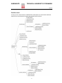
Setting up and evaluating a scenario
Setting up a scenario involves three phases: Defining the amount and composition of the waste to
be managed (Waste Generation), defining the source segregation scheme and the type of waste
collection (Waste Collection), and finally defining the managing of the separately collected waste
streams, maybe routed through several treatment steps before recovery and or final disposal
(Treatment, Recovery & Disposal). These steps must be defined so far that no significant waste
stream is left unmanaged in the system. The model allows for truncation of the waste flows and
for leaving out side streams if found appropriate for the problem being studied.
The evaluation of a scenario usually involves several steps:
Material flows: The model calculates all masses of waste entering a process and all solid
waste streams leaving a process, these be products or residues. The calculated mass
flows should be compared with the mass flows of the actual case being modeled. If
unacceptable discrepancies are observed, the model set up must be checked and
modified until a reasonable match with the real case is obtained.
Out-put composition: The model calculates the composition of the out-puts from each
treatment process, e.g. the bottom ash from the waste incinerator or the compost
composition from the composting plant. These calculated out-put compositions should be
compared with measured compositions, when possible, in order to assess how well the
model represents the real case. Adjustments in the model set-up may be needed.
However, it is not always possible to find real data on out-put composition that are
comparable to the ones calculated, because actual plants may simultaneously treat
several waste streams, which also will be reflected in the composition of the out-puts.
The LCI provides the account of all emissions and resource consumptions associated
with the waste management system. The LCI can be organized with respect to
substance, magnitude, or process. A sensitivity analysis can be made at LCI level.
Impact Potentials are calculated according the chosen LCA method. The impact
potentials can be related to substances or to processes and can be sorted according to
magnitude. A sensitivity ratio can be calculated at this level.
Normalization converts the Impact Potentials into person-equivalents. The normalized
impacts can be related to substances or to processes and can be sorted according to
magnitude. A sensitivity ratio can be calculated at this level
Weighting introduces a political weight on the normalized impact potentials. These
weighted values can be related to substances or to processes and can be sorted
according to magnitude. A sensitivity ratio can be calculated at this level
The final results may be expressed graphically or exported to Excel.
5
EASEWASTE
TECHNICAL UNIVERSITY OF DENMARK
Scenarios
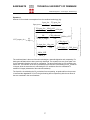
Possible routes
The way you can route the flows in EASEWASTE is hardcoded. This means that the individual
modules can only be followed by specific other modules that fit into them.
6
EASEWASTE
TECHNICAL UNIVERSITY OF DENMARK
Scenarios
User instruction
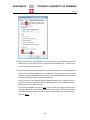
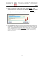
Adding a new scenario:
1. Select [Scenario] in the left pane window. Right click in the main window and press
[New] to create a new scenario. A new window will open.
2. Give the scenario a [name], usually the name of the project, city, country and year.
The year refers to year that the dataset is valid. Save the dataset before entering
further data.
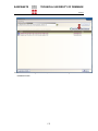
3. Choose a Scenario Type. Choose “single family”, “multi family” and SCBU” or any
combination hereof. The listed names are fixed and reflect the most common way of
using the model, but basically the issue is to choose how many parallel systems to
model simulateously. A maximum of three can be chosen. The three parallel
entrances may reflect urban setting with very different housing and waste collection
system, the same city in three different years, etc. The most simple is to work with
only one scenario type, because for each entrance the full scenario must be defined
individually.
For simplicity the following is described for “Single Family” only.
The scenario contains three phases in sequence: Waste Generation, Waste
Collection, and Treatment, Recovery & Disposal. The latter actually may contain
sequences of treatment, recover, etc.
4. [Waste Generation]: Choose a waste generation data set from the database that
opens up.. The data of the chosen dataset will appear in the window. The data can
be edited and saved in the window. However, the only value carried on is the Total
Waste [tonnes]. Choose a waste composition data set from the database that opens
up.. The data of the chosen dataset (material fraction distribution, chemical
composition as found under [View Composition]) will appear in the window. The data
can be edited and saved in the window. If any editing has been done you should
push [Update Data] before moving on. Editing does not affect the original databases,
only the data used in the scenario.
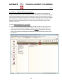
5. [Waste Collection]: This second phase is divided into Waste Sorting and Waste
Collection. Select first Waste Sorting and choose a data set on Sorting
Efficiencies from the database that opens up. The waste sorting data are used for
source segregation of waste. Even if no source segregation is anticipated a (any)
data set must be chosen.
6. Choose Number of Sorting Fraction from the scroll bar. A corresponding number of
name slots open up. The lower one is always called Residual Waste. The chosen
number of sorting fractions are named by selecting from the scroll bar. The names
available are those used in the chosen dataset on sorting efficiencies.
7. The [View] button allows for inspecting and editing the actual sorting efficiencies for
the actual sorting fractions. Editing must be followed by saving. Editing does not
change the data base, only the data used in the scenario. Note that the first column
represents the residual waste, and is calculated from the chosen sorting efficiencies
so that 100% of the waste is present in the scenario.
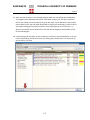
8. [Waste Collection]: The second half of the second phase is also called Waste
Collection. Here all the collection fractions including the residual waste are listed in
terms of the amount of waste to be collected separately. Select a Waste Collection
Technology for each Collection Fraction after double clicking in the respective box.
The [View] button can be used to inspect the fuel consumption (litre of diesel per
7
EASEWASTE
TECHNICAL UNIVERSITY OF DENMARK
Scenarios
tonne of wet waste) or the emission standards for the diesel combustion. Neither the
fuel consumption nor the combustion technology can be edited within the scenario.
Specifying the second stage Waste Collection and Transportation is optional. The
program can work without including this information, e.g. if only treatment
technologies are to be assessed
9. [Treatment, Recovery & Disposal] addresses the further transport and
management of the waste. For each Collection Fraction define a Distance for the
transportation (one way distance in km), a Transportation Technology, the type of
Treatment, Recovery & Disposal, and finally a Technology from the scroll bars
that represent the available databases. The routing of the waste from collection to the
first treatment step is not restricted by the model and should be chosen with due
consideration of the nature of the collection fraction.
10. For each Collection Fraction, after specifying the first treatment step, the [View]
button must be activated to specify the further routing of the waste after the first
treatment step. The routings available are locked in order to minimize the risk for
irrational management of the waste further downstream.
11. The technology activated by the [View] button should be inspected and edited to suit
the purpose. After editing, saving is needed before closing the technology window. At
the bottom of each technology window, residues and products are shown and should
be routed further by repeating steps 9 and 10 until no significant waste stream is left
within the waste management system
Editing an exiting scenario:
1. Open the scenario and edit any user-made specification. Save within each window
before closing the window. Warnings are offered if the number and type of collection
fractions are changed, because such changes will jeopardize the specifications made
under Treatment, Recovery & Disposal.
Comparison of two to four scenarios:
1. It is possible to compare up to four scenarios. This is done by selecting the scenarios
you are interested in by holding down CTRL and left clicking the scenarios of interest.
You then right click and choose LCA evaluation and choose one of the two
comparison options.
Technology evaluation within a scenario:
1. It is also possible to evaluate a technology within a scenario including the waste flow
set up in a scenario. This is done by choosing [Output] in the top bar and then
pressing [LCA Evaluation].
8
EASEWASTE
TECHNICAL UNIVERSITY OF DENMARK
Waste Generation - Waste Composition
2 Waste Composition
Document updated 29 November, 2007 by THC. Original document prepared by THC and controlled by CHR.
The module presents the composition of the waste at the point of generation in terms of the
weight distribution of material fractions and the chemical composition of each material fraction.
Each waste composition dataset may contain three different datasets regarding the distribution of
material fractions, but only one chemical composition is included. The waste composition is the
starting point for all routings of waste mass (e.g. in source segregation, material recovery and
incineration), for calculation of energy content and recovery, and for all calculations of in-put
specific emissions in the waste management system. The waste composition is also crucial for
the calculation of the stored toxicity.
Approach
The waste composition is a key factor in determining the potential for source segregation and
estimating energy recovery and emissions from the waste management system. Therefore it is
crucial that the waste composition used in the modeling closely reflects the actual waste.
Waste composition is described by the wet weight distribution of material fractions and the
chemical composition of each of these fractions. The three individual wet weight distributions for
municipal waste are a priori defined as representing single family housing [Single Family(%)]
multi-family housing [Multi Family(%)] and small commercial business units [SCBU(%)]. These
names cannot be changed, but they may represent any part of the waste management system
with respect to variations in material faction composition, source segregation or waste
management technology. EASEWASTE calculates flows and environmental assessment
individually for the three material fraction distributions.
The material fraction distribution represents the wet waste prior to any source segregation of any
kind. The 48 default material fractions are named according to the dataset on Danish household
waste 2003 presented by Riber et al. (2008). Material fractions can be renamed but this will affect
the source segregation efficiencies and transfer coefficients in all technology modules. If data are
not available for a fraction the composition values can be set at zero.
The chemical composition is in most cases based on dry matter (TS: Total Solids), but in some
cases on the basis of organic matter in terms of volatile solids (VS) or wet weight. The actual
units are shown in each case. In addition to the chemical substances also water content, heating
values (lower heating value on TS basis), methane potential are included. The chemical content
is total content, which means that sample digestion prior to analysis must be very effective and
any partial sample digestion is not recommended. If data are not available for a substance the
values can be set at zero.
Literature
Riber, C., Rodushkin, I., Spliid, H. & Christensen, T.H. (2007): Method for fractional solid waste
sampling and chemical analysis. International Journal of Environmental Analytical Chemistry, 87,
321-335.
Riber, C., Petersen, C & Christensen, T.H. (2008): Chemical composition of material fractions in
Danish household waste. (submitted).
9
EASEWASTE
TECHNICAL UNIVERSITY OF DENMARK
Waste Generation - Waste Composition
User instructions
A new dataset is established by:
1. Select [Waste generation] [Composition] in the left window pane of the screen.
2. Click the white sheet icon to make a new waste composition. It is also possible to modify an
existing dataset or make a copy of one.
3. Enter a [name] of the waste composition. Waste compositions in the EASEWASTE database
4.
5.
6.
7.
8.
9.
are named according to: waste type, country or region and year the data was collected, e.g.
Household waste [SF + MF], DK, 2003.
Enter the material composition using either the 48 predefined names or new names. A new
material fraction name is made by right clicking on a fraction name and select [Open] – then
the name can be redefined. This will take effect everywhere in your EASEWASTE program,
also in the saved scenarios; therefore this feature is rarely used.
The mass distribution of material fractions in percentages within each of the sub-systems are
entered in the three columns called [Single Family (%)], [Multi Family (%)], and [SCBU
(%)]. If the sum of all material fractions does not equal 100%, then you must adjust the
numbers so the sum of all material fractions is 100%.
Values for the chemical composition are entered in the remaining columns. The unit for each
substance is stated in the head row. It can be either % of wet mass, % of TS, or % of VS.
H2O plus TS is set to be 100 % of wet waste, and VS plus Ash is set to be 100% of TS. When
one of them is keyed in, the other is automatically calculated. C-biological plus C-fossil is also
set to be 100 % of C-total, but the value is given as %TS. These rules cannot be deviated.
In general, values are entered by selecting the cell pressing “enter” (or double click) and
entering the value. After entering by pressing “enter” the next cell to the right will be selected
and by using the arrows other directions can be chosen. Copy/paste works from one cell to
another by marking the value; selecting copy; choosing a new cell; and selecting paste.
Note! Most predefined technology datasets in EASEWASTE are based on 48 fractions. Thus,
a choice of more fractions will make the predefined technologies unavailable.
Data requirements
The user must assure that the waste composition reflects the actual waste, as this could be
crucial for the LCA results. The distribution of material fractions and the chemical composition of
each material fraction are highly correlated and should ideally be measured in the same
investigation. It is recommended to be very careful when data are mixed from different sources.
The sorting method of material fractions from waste is to some degree defining the chemical
composition of the sorted fractions and even though the name is identical the composition could
vary substantially.
10
EASEWASTE
TECHNICAL UNIVERSITY OF DENMARK
Waste Generation – Waste Quantity
3 Waste Quantity
Document updated November 29, 2007 by THC
The module presents the quantity of waste at the point of generation in terms of the wet weight.
Each waste quantity dataset may contain three different sets of data, for example, representing
three different sources of waste, collection systems, or years. The module offers help in calculating
the mass of wet waste. The amount of waste (wet tonnes of waste) for each set of data constitutes
the basis for all calculations within scenarios using the dataset.
Approach
The waste quantity is a key factor in modeling the waste management system. The model is linear
with respect to waste quantity. Therefore it is crucial that the waste quantity used in the modeling
closely reflects the actual waste management issues addressed.
Waste quantity is described by the wet weight. Three individual sources of wet weight for
municipal waste are a priori defined as representing single family housing [Single Family(%)]
multi-family housing [Multi Family(%)] and small commercial business units [SCBU(%)]. These
names cannot be changed, but they may represent any part of the waste management system with
respect to variations source, waste management technology, or years. For example the three sets
could represent Copenhagen 2007, Copenhagen 2012 and Copenhagen 2017. EASEWASTE
calculates flows and environmental assessment individually for the three sets of data
Waste quantity in EASEWASTE does not have a unit of time. EASEWASTE deals only with a
mass of waste. Since most data on waste quantity are associated with a time period (e.g. per year)
it is important in the documentation of the actual data to specify the time issues.
Often the waste quantity is based on number of housing units, number of persons per unit and the
unit generation rate per person. Data are entered via these parameters but only the final wet
weight is used in the calculations in the model.
Literature
No specific literature
User instructions
A new dataset is established by:
1. Select [Waste generation] [Waste quantities] in the left window pane of the screen.
2. Click the white sheet icon to make a new waste quantity dataset. It is also possible to modify
an existing dataset or make a copy of one.
3. Enter a [name] of the waste quantity dataset. Waste quantity datasets in the EASEWASTE
database are named according to: waste type, country or region and year the data was
collected, e.g. Household waste [SF + MF], DK, 2003.
4. Enter [No. of Units], [people/Unit], and [Waste] (the latter in kg/pers.) so they reflect the
actual waste generation or any combination that results in the amount of waste that should be
modelled (e.g. 1000 tonnes). Total Waste (tons) is the amount of wet waste used in the
further calculation.
11
EASEWASTE
TECHNICAL UNIVERSITY OF DENMARK
Waste Generation – Waste Quantity
Data requirements
The user must assure that the waste quantities represent the actual waste management issue
addressed.
12
EASEWASTE
TECHNICAL UNIVERSITY OF DENMARK
Waste Generation – Sorting Efficiencies
4 Sorting efficiencies
Document updated November 29, 2007 by THC. Original document prepared by THC and AWL and controlled by JAM.
The module deals with source segregation of material fractions within a waste type. The module
provides a database on how much of a material fraction is segregated into a sorting fraction
collected separately at the source (here named sorting efficiencies) and thus defines the separate
waste streams to be managed in a scenario. The sorting efficiencies represent the average
performance of the area modelled. If a fraction was defined as being subject to source segregation
and all citizens all the year followed the guideline 100%, then the sorting efficiency would be 100%.
Sorting efficiencies appear in two ways:
As a dataset under Waste Generation with a range of possible sorting fractions with
potentially a range of sorting efficiencies. The database should include realistic sorting
efficiencies for alternative source segregation schemes.
In the scenarios where the number of sorting fractions can be defined and the
corresponding sorting efficiencies can be selected from the above-mentioned database.
In the scenario the sorting percentages for each fraction are cumulative and the remaining waste
not defined as subject to source segregation is routed to residual waste in order to ensure mass
conservation.
Approach
At the source of waste generation it is important within a single waste type to define the waste
streams that shall be collected separately. This is done by defining sorting efficiencies for each
material fraction defined in the waste type. The sorting efficiency defines how much of the material
fraction is segregated into the defined sorting fraction in average for the area modeled. In this way
the sorting efficiency differs from the participation rate, because participating citizens may not
participate all year round and may not sort the waste 100% correct according to the sorting
guideline.
Source segregation should be defined to obtain a sound routing of the segregated fractions in the
waste management system, i.e. through collection, transport, treatment etc. Source segregation is
often introduced by providing the citizens with sorting guidelines specifying which material fractions
in the waste go into which sorting fractions (e.g. paper, packaging, organics, etc.). The sorting
efficiencies depend on the sorting fractions defined (e.g. as described in the sorting guideline given
to the citizen), on the collection system available (a full service system collecting the recyclables at
the house or must the citizen bring the source segregated material to a recycling station), and the
general engagement of the citizen (level of information, means of paying for waste service
etc.).These factors are however all correlated: A meaningful and clear sorting guideline requiring a
minimum of effort by the citizen combined with a collection system that makes it easy to deliver the
recyclables should give high sorting efficiencies (maybe 80-90%), while less user friendly systems
may have much lower sorting efficiencies.
In the Waste Generation database sorting efficiencies can be defined for a range of systems
relevant for an area. In the database the sorting fractions and efficiencies may represent
alternative systems, because in the scenario any combination of sorting fractions can be selected
from the database (note that you will get an error message, if you choose sorting options that
13
EASEWASTE
TECHNICAL UNIVERSITY OF DENMARK
Waste Generation – Sorting Efficiencies
together exceed 100% for one waste fraction). In the scenario the sorting fractions must be
complementary representing a realistic system, and the material fractions not included in the
source segregation and the part of the material fractions not successfully segregated at the source
are automatically routed to the residual fraction in order to ensure mass conservation at the
source.
Sorting efficiencies can also be used to include foreign items in a sorting fraction (e.g. cardboard
that mistakenly was placed in a newspaper sorting fraction)
Literature
No specific literature
User instructions
Adding a new dataset (outside the scenario):
1. Select [Waste Generation] [Sorting efficiencies] in the left window pane. Right
click in the main window and press [New] to create a new dataset. A new window will
open.
2. Give the dataset a [name]. Sorting efficiencies in the EASEWASTE database are
named according to: focus of the source segregation system, the name of the city,
country and year. The year refers to year that the dataset is valid. Save the dataset
before entering further data.
3. Define for “single family”, “multi family” and “SCBU” or only part of them which sorting
fractions should be included. This is done by right clicking and adding the needed
number of columns (click for each new sorting fraction). The names of the sorting
fractions can be defined by right clicking and choosing [Edit Fraction Name].
4. Alternative sorting fractions can be defined since there is no need to consider mass
conservation here. This is done in the scenario. For each material fraction a
percentages is defined showing how much of the material fraction (% of wet weight) in
average will go to the defined sorting fraction. This may also apply to contaminants
and mis-sorting
Supplementing an exiting dataset (outside the scenario):
1. Select [Waste Generation] [Sorting efficiencies] in the left window pane of the
screen. Click on an existing dataset.
2. File the edited dataset under a new name by “save as” .Give the edited dataset a
[name]
3. Right click on the dataset and add the additional sorting fraction (click for each new
sorting fraction). The names of the sorting fractions can be defined by right clicking
and choosing [Edit Fraction Name].
Use a sorting efficiency dataset in a scenario:
1. In a scenario, under “Waste Collection” , “Choose” the dataset for sorting efficiencies
that you want to use.
2. Define “Number of sorting fraction” by the scroll bar (Number = number of source
segregated sorting fractions plus the residual waste fraction).
3. Define the names of the sorting fractions as they appear by the scroll bar. The last
sorting fraction is always named “Residual Waste”.
14
EASEWASTE
TECHNICAL UNIVERSITY OF DENMARK
Waste Generation – Sorting Efficiencies
4. By clicking “View” the corresponding sorting efficiencies appear. The “residual waste
fraction” is calculated by the model to ensure mass conservation.
5. Close the window and move on with the modeling.
Editing a sorting efficiency dataset in a scenario:
1. In a scenario, under “Waste Collection” click “View” to see the original dataset.
2. Change any number in the sorting efficiencies and the model will recalculate the
“residual waste” fraction. Save before moving on with the edited dataset. The dataset
will remain changed in the scenario also when the scenario is opened later. The
original sorting efficiency dataset will not be changed.
Data requirements
Following issues must be considered when collecting data for creation of dataset with sorting
efficiencies:
The sorting guidelines available for actual systems with source segregation may be a
source of inspiration.
It is important to focus on how the sorting fraction is managed afterwards. How clean must
it be, is moisture a problem for storage etc. The material fractions to be included in a
sorting fraction must reflect this and respect the citizens’ ability to understand the
guideline.
Data from existing systems regarding collected tonnes and “mis-sortings” may be useful in
setting up realistic sorting efficiencies.
Technical calculations
Mass conservation is introduced in the scenario so that all waste in source separated fractions and
the residual fraction make up 100% of the mass.
Equation 1
The amount of a material fraction that is routed to the next technology (tonne); it is assumed that
the water content does not change:
Material_frac = Input_mass * Input_frac * Sorting_frac
Each material fraction is kept separate throughout the system, but is added up for routing a total
mass to the next technology.
Economics
Not yet available
Variables and Constants
Input_frac
Amount of each material fraction in %
Input_mass
Input of waste to the sorting system (tonne ww)
15
EASEWASTE
TECHNICAL UNIVERSITY OF DENMARK
Waste Generation – Sorting Efficiencies
Material_frac
Material_fraction sent on to a new technology (tonne
ww)
Sorting_frac
Amount of each input fraction sorted into a sorting
category in %.
16
EASEWASTE
TECHNICAL UNIVERSITY OF DENMARK
Waste Management – Waste Collection
5 Waste collection
Document updated November 28, 2007 by AWL. Original document prepared by AWL and HKL and controlled by THC
The module represents collection of waste in trucks in terms of the fuel consumption and the
exhaust emissions caused by the fuel combustion. Use of fuel is considered the predominant
environmental load from waste collection. The environmental load from producing and using bins,
sacks, containers and from producing and maintaining trucks is not included in the technology.
Collection is defined in terms of the fuel consumption per tonne of wet waste from the first stop on
the collection route to the final stop on the collection route. Fuel spent on driving from the garage to
the start of the collection route, driving from the final stop on the collection route to the unloading
point, and driving from that point back to the garage is considered part of transportation and can be
modelled in the transportation module. The emissions associated with combustion of the fuel are
obtained from the external process database.
Approach
Each waste collection dataset represents collection of a certain type of wet waste (mixed, residual,
paper, etc.) and is characterized by the type of container (size, type), the type of vehicle (size,
emission standards), and layout of the collection route within a defined neighborhood (density of
bins, bins per stop, traffic, and access to bins). The specific fuel consumption per tonne of wet
waste can be estimated from approaches suggested in the literature or by direct measurements,
e.g. Larsen et al. (2008) shows the measurements of collection of several kinds of household
waste.
Fuel and its combustion is the major environmental load from waste collection. The most important
exhaust emissions are carbon dioxide, sulphur dioxide and heavy metals, which are related to the
chemical composition of the fuel, and nitrogen oxides, carbon monoxide, non-combusted
hydrocarbons (NMVOC) and particles, which depends on the engine operations. Environmental
loads from infrastructure, wear on vehicles and maintenance of vehicles are not included.
The fuel consumption depends on parameters such as type of truck, engine size of the truck,
compaction of the waste, capacity use, distance between stops, amount of waste collected per
stop, and acceleration, speed and braking between stops. The fuel consumption of a vehicle is
also influenced by the type of road (whether it is urban or rural collection) and by the mechanical
bin lifting devices. The fuel consumption is expressed for a given combination of truck, route and
waste as an average consumption of diesel per tonne of wet waste. It is not necessary to obtain
data for all abovementioned parameters, as these are aggregated into one parameter for diesel
consumption. If fuel is spent locally on collection of waste by small tractors or by vacuum collection
systems the corresponding fuel consumption must be converted to fuel consumption per tonne of
wet waste and included in the waste collection fuel consumption. The default unit is liters of diesel,
but other types of fuel can as well be chosen, e.g. Nm3 gas or kWh electricity; all must be per
tonne of wet waste.
Production and maintenance of bins, containers and trucks are not included in this approach for
waste collection.
Literature
Larsen, A., Vrcog, M. & Christensen, T.H. (2008): Diesel Consumption in Waste Collection and
Transport. (in preparation).
17
EASEWASTE
TECHNICAL UNIVERSITY OF DENMARK
Waste Management – Waste Collection
User instructions
A new dataset is established by choosing a fuel combustion technology and a value for the fuel
consumption per tonne of wet waste:
12. Select [Waste Management] [Collection] in the left window pane of the screen.
13. To create a new waste collection technology, right click anywhere on the window and
select New. Provide a [name] for the technology. Collection technologies in the
EASEWASTE database are named according to: type of waste collected, the type of
residency or collection technology, city, country and year. The year refers to when the
main data behind the technology were collected, e.g. “Paper, drop-off-containers,
Aarhus, DK, 2004”. Save the technology before entering further data.
14. [Fuel combustion technology] is used for calculation of the environmental load from
production and combustion of 1 litre of fuel. It is an external process which is chosen in
the database. Any new combustion processes must be added in the external process
database.
15. [Fuel consumption] is the parameter value for the specific fuel consumption in a new
waste collection dataset. The default unit is liter of diesel per tonne of wet waste.
In a scenario, the waste collection dataset is chosen by double clicking in the cell [Waste
Collection Technology], located in the waste collection window under the waste collection sub
tab. The number and type of collection fractions are defined in the waste sorting tab.
Data requirements
Creating a new waste collection dataset requires two parameters:
The input data in [Fuel combustion technology] are external processes, which
should emphasize at least production and combustion of the fuel. Data on production
are most often included in LCI databases. Exhaust emissions from the combustion
process depends on engine technologies and operations and can be obtained from
standard tables on emissions or transport simulation software. Some emission
substances depend on the chemical composition of the fuel, while other depends on
operation of the combustion engine.
[Fuel consumption] can be measured directly on real collection schemes by following
a standard measurement procedure. Alternatively, the specific fuel consumption can
be estimated from the waste collection operator’s statistics on fuel consumption and
model estimates on how much fuel is used on transportation outside the collection
area, e.g. driving from the garage and back and between the collection area and the
point of unloading.
Technical calculations
Calculation of LCI tables for waste collection is performed in the Waste Collection Window.
Datasets for waste collection are given as fuel consumption per tonne of wet waste and are
multiplied with the mass of a chosen collection fraction. Within the dataset, the fuel consumption
parameter is multiplied with an LCI table for the chosen external process for fuel production and
combustion. The resulting equation is:
Equation 1
LCI _ col Output _ mass Ext _ LCI Fuel _ collect
18
EASEWASTE
TECHNICAL UNIVERSITY OF DENMARK
Waste Management – Waste Collection
Economics
Not yet available
Variables and Constants
Ext_LCI
LCI table of an external process (kg/tonne)
Fuel_collect
The fuel consumption parameter used in waste collection
(liter/tonne)
LCI_col
LCI table of waste transportation (kg/tonne)
Output_mass
Wet output mass from a collection fraction or a
technology (tonne)
19
EASEWASTE
TECHNICAL UNIVERSITY OF DENMARK
Waste Management - Waste transportation
6 Waste transportation
Document updated November 29, 2007 by AWL. Original document prepared by AWL and HKL and controlled by THC
The module represents transportation of waste by truck, ship and railway. Waste transportation is
defined as transportation of waste between treatment facilities after collection of the waste.
Collection is therefore not a part of the transportation, but it can be modeled separately in the
collection module. The datasets each includes a fuel consumption value expressed in the unit liters
of fuel per tonne of waste per traveled km as well as a process for production and combustion of
the fuel. The processes are obtained in the external process database. The most important
impacts from transportation are considered to be consumption of fuel and the exhaust emissions
caused by fuel combustion. Transportation can be added once in each step of the waste treatment
system.
Approach
Transportation represents the fuel consumption for the transport of the collected waste to the point
of unloading, e.g. at the treatment facilities or landfill. Transportation can be characterized by the
means of transportation (e.g. truck, ship or railway), capacity use, engine technology, etc. The
transportation can be assessed precisely if the transportation route between the collection point
and the point of unloading is known in terms of the physical distance between waste management
facilities. However, if the waste is exported, regionally or globally, the transportation means and
routes may vary significantly and estimates will be uncertain. Since transportation accounts for only
a minor part of the environmental impact from waste management, the modeling of it should be
kept simple. Therefore, only one type of transportation can be added between two waste treatment
facilities.
Fuel and its combustion is the major environmental load from transportation of waste. The most
important emissions are carbon dioxide, sulphur dioxide and heavy metals, which are related to the
chemical composition of the fuel, and nitrogen oxides, carbon monoxide and non-combusted
hydrocarbons (NMVOC) and particles, which depend on the operation of the engine and actual
emission standards. Emissions are regulated for road vehicles, for example by European Emission
Standards. Environmental loads from production and maintenance of means of transportation,
infrastructure and tire wear are most often not included.
The fuel consumption is expressed as a unit fuel consumption corresponding to the amount of fuel
used for transporting 1 tonne of waste a distance of 1 km. That has by default the unit
[liter/(ton·km)], but it could also be expressed in, e.g. Nm3 gas or kWh electricity, all per tonne of
wet waste per km. The fuel consumption depends on many different parameters such as type and
size of the means of transportation, volume weight of material, capacity use, combustion engine
technologies, and traffic conditions on the transportation route. All these conditions are aggregated
into one parameter for fuel consumption. Datasets for various kinds of transport are found in the
external process database.
The distance traveled for the waste is the length of a travel route in km from where collection was
complete and to the point of unloading. This one-way distance is also the distance in km used for
calculating the fuel consumption. This means that any fuel used on driving from the garage to the
collection area and from the point of unloading back to the garage should be accounted for in the
fuel consumption value.
21
EASEWASTE
TECHNICAL UNIVERSITY OF DENMARK
Waste Management - Waste transportation
Literature
No specific literature
User instructions
A new dataset is established by:
1. Select [Waste Management] [Transportation] in the left window pane of the
screen.
2. To create a new transportation technology, right click anywhere on the window and
select New. Provide a [name] for the technology. Transportation technologies that
refer to a specific kind of waste collection are named according to: the type of truck,
type of waste collected, type of residency or collection technology, city, country and
year. The year refers to when the main data behind the technology were collected, e.g.
“Collection truck, paper, drop-off-containers, Aarhus, DK, 2004”. Datasets for more
generic types of transportation should be named according to: the type of means of
transport, size, waste type, region, year, e.g. “Long haul truck, 25 tonne, generic,
global, 2007”. Save the technology before entering further data.
3. [Fuel combustion technology] is used for calculation of the environmental load from
production and combustion of 1 liter of fuel. It is an external process which is chosen
from the database. Any new processes must be added in the external process
database.
4. [Fuel consumption] is the parameter value for the specific fuel consumption in a new
waste transportation dataset. The default unit is liter of fuel per tonne of wet waste per
km.
In a scenario, the waste collection dataset is chosen in the cell [Transportation Technology] and
linked to a mass of waste either between collection and the first waste technology or between
successive waste technologies. The transportation distance is entered in the cell [Distance] in
connection with the chosen dataset. This distance is the one-way distance in km.
Data requirements
Creating a new waste transportation dataset requires two parameters:
The input data in [Fuel combustion technology] are external processes, which
should emphasize production and combustion of the fuel. Data on production are often
included in LCI databases. Exhaust emissions from the combustion process depends
on engine technologies and operations and can be obtained from standard tables on
emissions or transport simulation software. Some emission substances depend on the
chemical composition of the fuel, while other depends on operation of the combustion
engine.
The parameter value for [Fuel consumption] can be obtained in different ways.
Datasets for transportation by truck, ship and railway are found in various LCI
databases. These will most often include a value for fuel consumption that can be
converted to the default value liter per tonne per km. The value can also be calculated
in transport simulation software and linked to a combustion process. Other possibilities
are to perform measurements on real vehicles or to calculate it from operators’ fuel
consumption statistics.
22
EASEWASTE
TECHNICAL UNIVERSITY OF DENMARK
Waste Management - Waste transportation
Technical calculations
Calculation of LCI tables for transportation is done by multiplying the dataset with a mass of wet
waste and a given distance. Within the dataset, the fuel consumption parameter is multiplied with
an LCI table for the chosen external process for fuel production and combustion. The resulting
equation is:
Equation 1
LCI _ trans Output _ mass Ext _ LCI Fuel _ trans Dist
Economics
Not yet available
Variables
Dist
Waste transportation distance (km)
Ext_LCI
LCI table of an external process (kg/tonne)
Fuel_transp
The fuel consumption parameter used in waste
transportation (liter/tonne/km)
LCI_trans
LCI table of waste transportation (kg/tonne)
Output_mass
Wet output mass from a collection fraction or a
technology (tonne)
23
EASEWASTE
TECHNICAL UNIVERSITY OF DENMARK
Waste Management – Technologies – Ash Treatment
7 Ash Treatment
Document updated 08-01-2008 by AND. Original document prepared by THA and controlled by THC.
The module represents treatment of ashes originating from thermal treatment of waste. The
module focuses on the treatment process itself. Treated ashes can be routed further to material
utilization or landfilling. Examples of ash treatment processes that the module may be used to
evaluate are: extraction processes, chemical stabilization processes, solidification processes, and
thermal treatment processes. All processes produces as minimum a single solid output that may
either be utilized or landfilled. Transfer coefficients can be defined for each output material.
Approach
The module represents treatment of ashes from thermal treatment of waste. The module can be
used for modelling of various kinds of ash treatment, e.g. extraction processes, chemical
stabilization, solidification, as well as vitrification and melting of the ashes. Useful solid outputs
from the ash treatment process may be routed further to material utilization and/or landfilling.
Each ash treatment dataset represents a full treatment plant as defined by the type of process
and technology used. The module includes process-specific auxiliary material and energy use as
well as process-specific emissions originating from the process itself and based on the ash input
quantity (i.e. ash routed from a thermal treatment plant). Transfer coefficients are used to link
substances in the ash input and with substances in the defined material outputs, e.g. the treated
residues and any secondary waste streams.
Process-specific and input-specific emissions are categorized according to the receiving
environmental compartments (air, surface water, soil) and/or material outputs. The transfer
coefficients are defined for each output material fraction (the module only has a single input) and
are distributing the input to the defined outputs. All transfer coefficients should add up to 100 %.
As ashes may be quenched or wetted at the thermal treatment plant in order to avoid dusting
during transportation, the dry matter content specified in the thermal treatment module (TS in %
of WW) for an individual material output is carried over to the ash treatment module and
automatically gives the amount of TS and WW. As the treated ashes may also contain water, a
dry matter content can be specified for each material output defined.
Literature
Astrup T, Fruergaard T, Christensen TH: Life-cycle assessment of residue treatment
technologies: methodology. (In preparation).
Fruergaard T, Astrup, T. Life-cycle assessment of residue treatment technologies: case-studies.
(In preparation).
User instruction
25
EASEWASTE
TECHNICAL UNIVERSITY OF DENMARK
Waste Management – Technologies – Ash Treatment
A new dataset is established by:
1. Give the technology a [name]. In the EASEWASTE database ash treatment plants
are named according to: Process type, name of the plant or process (if any), city,
country and year. The year refers to when the main data behind the technology were
collected, e.g. “Chemical stabilization, Ferrox, Copenhagen, Denmark, 2006”. Save
the technology before entering further data.
2. One to ten outputs are defined [Number of Outputs] in the top part of the screen.
3. The type/name of the outputs is defined in the bottom of the screen [Output
Materials].
4. Specify the TS-content of each output, i.e. the dry-matter content of the output after
the ash treatment process ([TS in % of WW] of each output).
5. For all outputs and substances specify [Transfer Coefficients].These coefficients
represent the percentage of an individual [substance] in the input ash being
transferred to the defined outputs. Unlike the thermal treatment module, the ash
treatment module does not include input specific air emissions and does not allow
[Transfer Coefficients] to be defined for air emissions. In this module, air emissions
(if any) should be specified as process specific emissions.
6. [Input – Material and Energy] is used to list materials and energy that are
consumed in the ash treatment process and the operation of the facility (process
specific data).
7. [Input – Resources and Raw Materials] is used to list materials that are used in the
process but are not contributing to any significant emissions during their extraction,
production, transport and consumption. These materials are only counted as
resource use.
8.
[Output – “Compartment”] is used to list the direct process specific emissions to
various environmental compartments (kg/tonne of wet waste).
9. In a scenario, the user can route the [Output materials] to either material utilization
or landfilling.
Data requirements
When collecting data for creating a new ash treatment process the following important
parameters should be considered:
[Input – material and energy] may have a significant impact on the overall evaluation of
the ash treatment process, in particular when comparing different treatment processes,
as for example, energy consumptions can indirectly contribute with relative large impacts.
Relevant units are typically kg, kWh, l (liter) or MJ /tonne.
[Output – “Compartment”] represent direct emissions from the process itself; these
emissions may for some processes be significant compared with the impacts related to
materials and energy consumptions. Required unit is kg/tonne.
26
EASEWASTE
TECHNICAL UNIVERSITY OF DENMARK
Waste Management – Technologies – Ash Treatment
[Transfer coefficients] are typically of less relative importance for the evaluation of the
ash treatment process itself; however the coefficients may have significant impact on
emissions from the treated ashes when routed to material utilization or landfilling as these
coefficients define the composition of the treated ashes. It should however be realized
that a good mass balance of a treatment plant is necessary, in particular to make sure
that all relevant mass flows are accounted for. The unit of transfer coefficients is a
percentage of the input.
Technical calculations
The main calculations performed in the ash treatment module are shown below. For calculations
regarding definition of the ash input to the module, please refer to the information available for the
thermal treatment module.
Equation 1
The amount of a substance in a specific material output (such as treated ash) is calculated. The
word “output” in the equation below may be exchanged with the name of specific outputs (e.g.
treated ash, secondary waste stream, etc.) and the word “substance” may be changed to a
specific substance (e.g. Cd, Cu, etc.).
Subs_output = Input_mass*TS_input*Sub_input*Subs_output_TFC
The input mass of ashes is converted into TS and the fraction of a specific substance in % of TS
in the ash is calculated. This is then multiplied with the transfer coefficient for the material output
in question thereby yielding the amount of a substance in the specific output.
Equation 2
The amount of a given output is calculated from routing of the dry waste amount, TS % in the
output defined in the technology window:
Output_mass = input_mass*TS_input*TS_output
The mass of an output is calculated as the TS in the input multiplied with the TS fraction routed to
the output in question. This TS fraction is specified within the transfer coefficients window. Please
note that the user can specify the dry matter content ("Output_TS") of the output itself as it leaves
the ash treatment process (i.e. to account for water added to avoid dusting, etc.). This value does
not affect routing of mass to the individual outputs.
Equation 3
LCI calculation for a substance is the sum of all process specific emissions and the LCI of all
external processes. The overall equation is as follows:
LCI =
Input_mass ×
Process_amount × Ext_LCI
processes
The LCI for ash treatment includes process specific emissions to air, soil and water as described
in the equation above. Any use of materials or energy (like additives or electricity) is added to the
27
EASEWASTE
TECHNICAL UNIVERSITY OF DENMARK
Waste Management – Technologies – Ash Treatment
LCI as well with the related emissions. For further description of the equation see the document
on LCI.
Equation 4
It should be noted that substance concentrations in the outputs are not part of a LCA method but
are provided in EASEWASTE to facilitate the evaluation and comparison of results with
monitoring data usually expressed in concentrations.
The output substance concentration is defined as the ratio between total mass of a material
output and the quantity of a substance routed to this material output (e.g. grammes of mercury
per tonne of treated ash).
Output_subs =
Subs_output
Output_mass
Economics
The general approach and user instruction for the economic part are described in the feature
document “Documentation: Economics”.
Variables and Constants
Variables
Ext_LCI
LCI table of a external process (unit/tonne)
Input_mass
Input of ash to the technology (tonne ww)
LCI
LCI table of a treatment process (kg/tonne)
Output_mass
Mass of a material output in TS (tonne)
Output_TS
User defined TS in percent for an output (%)
Process_amount
??
Sub_input
Amount of a substance as a percent of TS in the incoming
ashes (%)
Subs_output
Amount of a substance in a material output (tonne)
Subs_output_TFC
Transfer coefficient in percent for a substance to a given
material output (%)
TS_input
Percent of total solids (TS) in the incoming ashes (%)
TS_output
Percent of total solids (TS) in a material output (%)
28
EASEWASTE
TECHNICAL UNIVERSITY OF DENMARK
Waste Management – Technologies – Biotechnology
8 Biotechnology:
Biogas & Composting
Document updated November 28, 2007 by ALB. Original document prepared by ALB and controlled by JAM.
The module represents biological conversion of waste resulting in emissions to air, water and soil
as well as solid outputs and for anaerobic digestion also in energy production. The module
addresses degradation of organic matter, transfer of materials to defined outputs and any process
specific emission to air, water and soil. Use of the degraded waste in terms of compost or digest
is not included in the module. Any solid output must be routed further downstream. The module
focuses on composting, anaerobic digestion or a combination hereof. The module may potentially
also be used for biotechnological production of ethanol, hydrogen and methane gas for a market.
Based on the chemical composition, water content and methane potential of the material fractions
present in the input waste, the module calculates the biogas production (if any) for a defined
degradation rate, composition of outputs based on degradation of organic matter and materialbased transfer coefficients for defined outputs. Energy recovery, process specific emissions, offgas cleaning and losses of methane, nitrous oxide and ammonia can be specified. The type of
energy production avoided as a consequence of the energy recovered by the anaerobic digestion
must be specified to provide crediting of saved emissions and resource use.
Approach
Each biotechnological treatment dataset represents a full plant, including the technology of the
plant and the operation of the plant. If supplementary technologies, e.g. additional screening of
compost or magnetic metal removal, are needed, this can only be modelled by establishing a new
dataset where the considered add-on-technology is an integrated part of the dataset.
The module employs process-specific (mass per tonne of waste processed) material and energy
use as well as process-specific emissions. Process-specific emissions are categorized according
to the receiving compartment (air, surface water, soil, etc.). The degradation of the organic waste
is user defined and is expressed as percent degradation of volatile solids (VS) for each material
fraction by composting (aerobic process) and/or digestion (anaerobic process). Ash is not
degraded during biologic process, (i.e., the degradation coefficient for this fraction should be set
to zero). Transfer coefficients are used to transfer the non-degraded part of each material fraction
to defined outputs. The number and type of outputs can be specified for each individual
technology. The transfer coefficients are mass conserving (after degradation) and, considering all
outputs, add up to 100%.
Other non-solid outputs, emissions and pollution control devices are specific for the chosen
treatment among three technologies: composting, anaerobic digestion and a combination hereof.
The composting module includes a sub-module for emissions to air of nitrogen-compounds and
carbon-compounds. The total amount of nitrogen lost (as % of total N) and its distribution among
ammonia (NH3), nitrous oxide (N2O) and nitrogen (N2) is user specified. The amount of methane
released to the atmosphere, which depends on how the plant is operated, is also user defined as
a percent of the degraded C. The module calculates by default the degraded C and CO2 emission
to air using the degradation percentages specified by the user. These gaseous emissions can be
29
EASEWASTE
TECHNICAL UNIVERSITY OF DENMARK
Waste Management – Technologies – Biotechnology
treated in a gas-cleaning device (e.g. biofilter). Removal efficiencies (as percent) for NH3, N2O
and CH4 can be specified.
Anaerobic digestion has biogas as an output. Methane production is calculated based on
methane potentials included in the waste composition and the VS degradation specified by the
user. The methane content in the biogas is also user defined. Unburned CH4 is the amount of
methane lost in the process due to imperfect gas-tightness of reactor and pipes, incomplete
combustion, etc. It is defined as percent of produced CH4 (and not produced biogas!).
The module calculates the energy content of the biogas based on its methane content and,
through user-specified energy recovery (to be defined in a separate window as percent of the
energy content in the produced biogas), calculates the electricity and/or heat recovered. The user
must specify the avoided energy production in order to obtain the credits for saving in resource
use and emissions. The energy recovery is the gross energy recovery, since the plant’s own use
of energy is accounted for in the tables on material and energy input.
If the combined composting and anaerobic digestion module is chosen, all these features are
present in the same window and a degradation table with two columns is to be defined, one
related to anaerobic digestion and the other to composting.
Normally, the input waste for these technologies will be source-sorted organic household waste.
EASEWASTE, however, also includes the possibility to insert a Material Recovery Facility (MRF)
before the biotech module to model separation of different material fractions in unsorted waste.
Literature
Hansen, T.H., Sommer, S.G., Gabriel, S. & Christensen, T.H. (2006) Methane Production during
Storage of Anaerobically Digested Municipal Organic. Journal of Environmental Quality 35: 830–
836.
Hansen, T.H., Svärd, Å., Angelidaki, I., Schmidt, J.E., la Cour Jansen, J. & Christensen, T.H.
(2003) Chemical characteristics and methane potentials of source-separated and pre-treated
organic municipal solid waste. Water Science and Technology 48: 205–208.
Hansen, T.H., Schmidt, J.E., Angelidaki, I., Marca, E., la Cour Jansen, J., Mosbæk, H. &
Christensen, T.H. (2004) Method for determination of methane potentials of solid organic waste.
Waste Management 24: 393–400.
Boldrin, A., & Christensen T.H. Life Cycle Assessment Models for Biowaste Management (in
preparation).
User instructions
A new dataset is established by:
1. Select [Waste Management] [Technologies] [Biotechnology] in the left
window pane of the screen.
2. Give the technology a [name]. In the EASEWASTE database biotechnologies are
named according to: Type of treatment, technology and waste, city, country and year.
The year refers to when the main data behind the technology were collected, e.g.
30
EASEWASTE
TECHNICAL UNIVERSITY OF DENMARK
Waste Management – Technologies – Biotechnology
“Anaerobic digestion (household waste+green waste), “city”, “country”, “year”. Save
the technology before entering further data.
3. The type of treatment is defined [Type] in the top part of the screen. Three
alternatives are available: Anaerobic Digestion, Composting, Anaerobic &
Composting.
4. The degradation percentages are defined in [Degradation] for each material fraction
in the waste composition. In case of anaerobic digestion, the percentage is to be
interpreted as methane yield based on the methane potential, e.g., 60% degradation
of the vegetable food waste fraction means that the methane yield is 60% of the
methane potential of this waste fraction. In case of composting the number is to be
interpreted as percent of VS degraded during the process. In the combined
technology two columns are to be defined. The first column reporting the methane
yield during the anaerobic stage and the second defining VS degradation during
composting, their sum can theoretically exceed 100 %.
5. One to eight outputs are defined [Number of Outputs] in the top part of the screen.
6. The type/name of the outputs is defined in the bottom of the screen [Solid Outputs Output materials]. The TS content of each of the outputs must be specified ([TS in
% of wet weight] of each output).
7. The [Arrow] button placed beside [Number of Outputs] opens a new window where
[Distribution of TS after Degradation] are defined for each substance for all
outputs and represent the percent of the [substance] in each material fraction
transferred to the defined outputs. There is no distinction between ash and VS.
8. Depending on technology type chosen at point [1], several other parameters are to
be defined:
a. For anaerobic digestion the [methane content in biogas - % of CH4] and
[Unburned methane - % of CH4 produced]. ([Methane production – Nm3]
and [Energy in biogas – MJ] are calculate by the module). [Biogas
Utilization] is used to define the technology used for biogas combustion
(columns) and the energy substituted (lines). As the recovered energy refers
to a specific technology, a single percentage per line can be entered. The
sum of all percentages corresponds to the total recovery efficiency of the
energy contained in the biogas.
b. For composting the size of nitrogen-emissions as [Total N – loss - % of
Total N] and its distribution [Distribution of N – loss % - Ammonia NH3],
[Distribution of N – loss % - Nitrous Oxide N2O], [Distribution of N – loss
% - Nitrogen N2]. For carbon-emissions only the methane loss has to be
defined [CH4 - % of Degraded C], while CO2 is calculated by the module. If
gas cleaning devices are present, additional parameters to be defined are
the removal efficiencies (in percent) for the single gases: [NH3 - %
Removal], [N2O - % Removal], [CH4 - % Removal].
c. For combined technology all the parameters at both 7.a and 7.b have to be
defined.
9. [Input – material and energy] is used to list materials and energy that are
consumed in the biological process and the operation of the facility.
31
EASEWASTE
TECHNICAL UNIVERSITY OF DENMARK
Waste Management – Technologies – Biotechnology
10. [Input – resources and raw materials] is used to list materials that are used in the
process but are not contributing to any significant emissions during their extraction or
production, transport and consummation. These materials are only accounted for as
resource use.
11. [Output – Compartment] is used to list the direct process specific emissions to
various environmental compartments (kg/tonne of wet waste).
In a scenario, the user must route all outputs (except emissions to air) to further downstream
technological modules including a specification of the means of transport and transport distance.
The routings available appear in separate documentation file on the EASEWASTE website.
Data requirements
When collecting data for creating a new biological treatment technology there are a number of
crucial parameters:
[Degradation] has large impact because the conversion of VS determines the biogas
production (in case of anaerobic digestion) or the emissions of NH3, N2O and CH4
(composting).
[Unburned methane - % of CH4 produced] influences the impact on global warming.
Although measured data for this parameter are usually not available, for an average well
functioning plant this value should be fairly low (a few percent).
The amount and distribution of N-compounds and C-compounds in [Composting] can
have an impact on the assessment.
[Biogas Treatment] regarding the recovered energy is also very important. Both in terms
of the percentage of energy recovered and in terms of the type of energy recovered. It
has a significant impact whether the substituted energy is based on coal, gas or an
energy mix. The choice of a substitution process for the electricity production might often
be based on regional consensus on which process is substituted, since electricity often is
fed into a transnational grid. Selecting a substitution process for heat production delivered
to a local district heating grid requires detailed information on the alternative production
processes in the distribution net. In some cases a process representing the local heat
substitution will not be present in the database and specific information must be gathered
and a new process must be entered in the database for external processes.
[Gas Cleaning] in composting can substantially decrease the environmental impact of
gas emissions, as compounds with high impact can be removed or transformed to less
harmful substances. On the other hand, studies have shown that N2O can actually be
produced in biofilters. In this case a negative removal coefficient for N2O is defined.
[Transfer coefficients] have a large impact on the overall evaluation of the technology,
in particular the transfer coefficients controlling the amount of heavy metals released to
the compost fraction. It is therefore very important to obtain reliable data on transfer
coefficients. Information on chemical characterization of all outputs from the technology
as well as a precise mass balance is pre-requisite to make good estimates of the transfer
coefficients.
[Methane content in biogas - % of CH4] is an important parameter for anaerobic
digestion, as equations for mass balance, carbon balance and VS degradation are based
on it. When possible, it is recommended to use values measured at the real plant under
assessment.
32
EASEWASTE
TECHNICAL UNIVERSITY OF DENMARK
Waste Management – Technologies – Biotechnology
Beside this, a parameter highly influencing the impact of biological treatments is the content of VS
in the waste, because methane production in case of anaerobic digestion and emissions of
greenhouse gases in case of composting are directly related to this parameter.
Technical calculations
The main calculations performed in the biological treatment module are shown below.
Calculations that are necessary for generating data on the waste fed to the technology are not
shown, as these calculations are identical to those specified for the out-put from the preceding
technological modules. Most of the equations are working only inside a scenario. Every equation
is contained in a summation sign, meaning that the calculation is iterated for each material
fraction defined in the waste composition and the results are aggregated. In those equations
using an input in tonnes and calculating the result in kilograms, a factor 1000 is used for the
conversion.
Equation 1
Amount of total carbon emitted to the atmosphere during the anaerobic digestion (kg):
Input_frac TS_input_frac VS_input_frac
×
×
100 ×
100
100
Meth_yield
C_output_air = Input_mass ×
×CH4_pot
material fraction
100
×Molar_C
× CH4_%_biogas
×Vol_idealgas
100
Carbon is contained in the biogas in different forms and from there emitted to atmosphere. The
assumption is that the carbon degradation (and C-release to the atmosphere) is proportional to
the methane yield. Methane yield is a function of the methane potential of the specific fraction and
the VS degradation rate.
Multiplication of the upper terms of the fraction calculates the amount of produced methane.
Using the content of methane in the biogas (user defined) the whole fraction calculates the
amount of carbon contained in the biogas and hence emitted to atmosphere.
Equation 2
Amount of CO2 emitted to atmosphere from anaerobic digestion (kg):
Input_frac TS_input_frac VS_input_frac
×
×
100 ×
100
100
Input_mass ×
Meth_yield
material fraction
×CH4_pot
100
×
CO2_output_air =
Vol_idealgas
100
CH4_unburned
×Molar_CO2
100
CH4_%_biogas
33
EASEWASTE
TECHNICAL UNIVERSITY OF DENMARK
Waste Management – Technologies – Biotechnology
As in (Hansen et al., 2006) the assumption is that methane production from anaerobic digestion is
proportional to degraded volatile solids (VS). Biogas produced during anaerobic digestion is
mainly composed of methane and CO2. The CO2 emitted to atmosphere is the sum of the CO2
contained in biogas and that resulting from combustion of the methane contained in the biogas.
The first bracket calculates the amount of methane produced during the anaerobic digestion
stage. The first term in the second bracket (multiplied by Molar_CO2) calculates the amount of
CO2 contained in the biogas, while the second terms calculates the amount of CO2 produced form
the methane combustion.
Equation 3
Amount of CH4 produced in anaerobic digestion which is not burnt but emitted to the atmosphere
(kg):
Input_frac TS_input_frac VS_input_frac
×
×
100 ×
100
100
CH4_output_air = Input_mass ×
CH4_unburned Molar_CH4
material fraction Meth_yield
×CH4_pot×
×
×
100
100
Vol_idealgas
The methane produced during anaerobic digestion is burnt and hence released to the
atmosphere as CO2. A percentage of it is anyway escaping as fugitive methane loss.
The multiplication of the first 6 terms calculates the amount of methane produced. The second
last term accounts for the unburned methane.
Equation 4
Energy content in the methane produced in anaerobic digestion and burned for energy recovery
(MJ):
Input_frac TS_input_frac VS_input_frac
×
×
100 ×
100
100
Meth_yield
CH4_unburned
Energy_process = Input_mass × ×
×CH4_pot× 1×
100
100
material fraction
×Energy_CH4× Prod_eff_avoid
100
Substitution of an external process due to energy production is defined by a substitution process
and a related percentage expressing the efficiency of the energy recovery process. The overall
available energy amount is a multiplication of the methane produced by anaerobic digestion
(subtracted by the unburned methane) and the specific energy content of methane. The energy
substitution is then calculated by multiplying the available energy with the substitution processrelated production efficiency. The equation is valid also in the case of combined technology.
34
EASEWASTE
TECHNICAL UNIVERSITY OF DENMARK
Waste Management – Technologies – Biotechnology
Equation 5
Amount of total carbon emitted to the atmosphere during the composting process (kg):
Input_frac TS_input_frac C_input_frac
×
×
100 ×
100
100
C_output_air = Input_mass ×
material fraction Deg_rate
×1000
×
100
The assumption is that carbon degradation (and C-release to the atmosphere) is proportional to
both the carbon content in the waste and the VS degradation. The degraded carbon is emitted to
the atmosphere in different gaseous forms. Multiplication of the first four terms calculates the
amount of carbon contained in the feedstock to the process. The second two terms calculate the
amount of VS degraded. The multiplication of all of them gives the amount of carbon emitted to
the atmosphere.
Note: the equation is based on total carbon. Ideally, the release of fossil carbon and the impact
related to it should be calculated separately. Anyway, this is a very small issue, as material
fractions such as organic waste have a relatively small content of C-fossil and, moreover,
degradation of C-fossil during the processes under consideration is insignificant.
Equation 6
Amount of CO2 emitted to atmosphere during the composting process (kg):
CH4_degr_C CH4_degr_C CH4_clean
CO2_output_air = C_output_air 1
+
×
100
100
100
Molar_CO2
Molar_C
In the composting process CO2 is produced from degradation of organic matter under aerobic
conditions or from degradation of CH4 (or other volatile organic molecules not included in the
model) in the gas cleaner. The first term of the sum contained in the brackets account for CO2
directly from composting, while the second one accounts for the CO2 from the gas-cleaning
device.
35
EASEWASTE
TECHNICAL UNIVERSITY OF DENMARK
Waste Management – Technologies – Biotechnology
Equation 7
Amount of methane emitted to atmosphere during composting process (kg):
CH4_output_air = C_output_air
CH4_degr_C CH4_clean Molar_CH4
1
100
100
Molar_C
Composting can result in methane emissions due to transient anaerobic conditions in the
compost matrix. The first term of the equation is the total carbon emitted to air and previously
calculated. The second term calculates the percentage of the carbon emitted as CH4. This
coefficient is user-defined and might depend on the specifics of the facility. The third term is
accounting for the gas cleaning.
Equation 8
Amount of total carbon emitted to the atmosphere from the combined technology (kg):
Input_frac TS_input_frac
×
100 ×
100
VS_input_frac× Meth_yield ×CH4_pot
100
100
C_output_air = Input_mass ×
×Molar_C+
CH4_%_biogas
material fraction
×Vol_idealgas
×
100
C_input_frac Deg_rate
×
×1000
+
100
100
The combined plant is the sum of the two technologies: anaerobic digestion and composting. For
both types calculations have been previously described. The equation is a sum of two parts: one
for the anaerobic digestion and one for composting.
The first term of the sum (in brackets) in the second line is accounting for C contained in the
biogas (as product of degradation process), calculated using the methane content in biogas (user
defined). The third line is calculating the carbon degraded during composting and emitted to air
(in different forms).
36
EASEWASTE
TECHNICAL UNIVERSITY OF DENMARK
Waste Management – Technologies – Biotechnology
Equation 9
Amount of CO2 emitted to atmosphere from the combined technology (kg):
Input_frac TS_input_frac
×
×
100
100
VS_input_frac Meth_yield
×
×CH4_pot
100
100
×
Vol_idealgas
+
100
CH4_unburned
×
×Molar_CO2
CH4_%_biogas
100
CO2_output_air=
material_fraction
×
CH4_degr_C
+
C_input_frac Deg_rate 1100
×
×
×
CH4_degr_C CH4_clean
100
100
×
+
+
100
100
Molar_CO2
×
Molar_C
Input_mass×
The combined plant is the sum of the two technologies: anaerobic digestion and composting. For
both types calculations have been previously described. The equation is a sum of two parts: one
for the anaerobic digestion and one for composting. The terms contributing to CO2 emissions are
hence four. The first term of the sum (in brackets) in the third line is accounting for CO2 contained
in biogas, while the second term is calculating the CO2 emissions from the combustion of
methane in biogas (subtracted of the unburned methane).
The fourth line is calculating the CO2 emissions from composting, as produced from the process
in itself and the degradation of CH4 in the gas cleaning device respectively with the two terms in
the sum contained in the round brackets.
37
EASEWASTE
TECHNICAL UNIVERSITY OF DENMARK
Waste Management – Technologies – Biotechnology
Equation 10
Amount of CH4 emitted to atmosphere from the combined technology (kg):
Input_frac TS_input_frac VS_input_frac Deg_rate
100
100
100
100
+
CH4_pot CH4_unburned Molar_CH4 ×1000
100
Vol_idealgas
CH4_output_air = Input_mass ×
C_input_bio_frac Deg_rate
material fraction Input_frac TS_input_frac
100
100
100
100
+
× CH4_degr_C Molar_CH4 × 1- CH4_clean ×1000
100
Molar_C
100
The combined plant is the sum of the two technologies: anaerobic digestion and composting. For
both types description on how calculations are performed for the single plant has been previously
provided. The equation is a sum of two parts: one for the anaerobic digestion and one for
composting. The first term of the sum is accounting for CH4 contained in biogas and not burned
but released to atmosphere, while the second term is calculating the CH4 produced during the
composting process and not removed by the gas cleaning device.
Equation 11
Total N emitted to atmosphere during composting (kg):
Input_frac TS_input_frac
×
100 ×
100
N_output_air = Input_mass×
material fraction N_input Total_N_Deg_rate
×
×1000
×
100
100
The equation is valid also for the combined technology. In that case the input mass is the output
from the anaerobic reactor transferred to the composting facility.
The first five terms are calculating the amount of nitrogen contained in the input material. The
degradation rate is based on total nitrogen and is user defined. This degradation rate can be
estimated with a nitrogen balance on the plant.
The nitrogen is then released to atmosphere in different forms. The amounts of ammonia and
nitrous oxide emitted are calculated according to the next equations. In each of them, the second
term is user defined as the percentage of degraded N emitted in the specific form. The last term
accounts for the gas cleaning device.
NH3_output_air = N_output_air
NH3_degr_N Molar_NH3 NH3_clean
1
100
Molar_N
100
N2O_output_air = N_output_air
N2O_degr_N Molar_N2O N2O_clean
1
100
Molar_N2
100
Equation 12
38
EASEWASTE
TECHNICAL UNIVERSITY OF DENMARK
Waste Management – Technologies – Biotechnology
Amount of outputs from anaerobic digestion (tonnes in ww):
_
(
_
∗∑
_
100
∗ 1 −
_
∗
_
100
ℎ_
100
4_%_
100
=
100
∗
_
∗(
∗
ℎ_
100
4_
∗
_
_
_
100
_
∗
_
+
_
_
100
_
∗ 1.89 )
1000
_
It is assumed that degradation of VS is proportional to the carbon degradation.
Using the total solids (TS), the equation is calculating the output from the process. TS in the input
material are calculated with multiplication of the first three terms. The sum in the internal square
brackets is accounting for the ash content (which is not degraded) and the amount of VS
contained in the output after degradation has taken place. The multiplication of 1.89 is the TS loss
per kg CH4 formation. The last term is accounting for the distribution of TS among different
outputs. The denominator is converting from total solid (TS) to wet weight. The total solid content
is user defined.
Equation 13
Amount of outputs from composting (kg in ww):
Ash_input_frac
+
100
Input_frac TS_input_frac
100
100-Deg_rate VS_input_frac
100
Input_mass×
100
100
material fraction
Subs_output_TFC_frac
100
Output_mass =
Output_TS
100
Using the total solids (TS), the equation is calculating the output from the process. TS in the input
material are calculated with multiplication of the first three terms. The sum in the internal brackets
is accounting for the ash content (which is not degraded) and the amount of VS contained in the
output after degradation has taken place. The last term is accounting for the distribution of TS
among different outputs. The denominator is converting from total solid (TS) to wet weight. The
total solid content is user defined.
39
EASEWASTE
TECHNICAL UNIVERSITY OF DENMARK
Waste Management – Technologies – Biotechnology
Equation 14
Amount of outputs from combined technology (tonnes in ww):
_
(
_
∗∑
∗ 1 −
_
100
∗
_
ℎ_
100
_
100
4_%_
100
∗
∗
=
100
∗
_
∗ (
ℎ_
4_
_
_
_
_
100
∗
100
_
+
_
_
∗ 1.89 −
1000
_
100
_
100
_
Using the total solids (TS), the equation is calculating the output from the process. TS in the input
material are calculated with multiplication of the first three terms. The sum in the internal square
brackets is accounting for the ash content (which is not degraded) and the amount of VS
contained in the output after degradation has taken place, after both anaerobic digestion and
composting. The multiplication of 1.89 is the TS loss per kg CH4 formation. The last term is
accounting for the distribution of TS among different outputs. The denominator is converting from
total solid (TS) to wet weight. The total solid content is user defined.
Equation 15
Amount of nitrogen in the output from composting or combined technology (kg):
Input_frac TS_input_frac N_input
×
×
100 ×
100
100
N_output = Input_mass
material fraction 100-Total_N_deg_rate Subs_output_TFC_frac
×
×1000
×
100
100
The calculation of the output composition is presented here. For biological treatments
degradation depends on the considered compound (some compounds such as heavy metals are
not degraded at all) and the process (aerobic-anaerobic, etc). Therefore, it is not possible to
calculate the composition of the outputs from the treatments with a single equation.
The equation calculates the amount of nitrogen not lost during the process and still contained in
the output material from a composting plant or a combined technology. The first four terms
calculate the total nitrogen in the input. The fifth term accounts for the nitrogen not degraded. The
second last term is accounting for the distribution of TS among different outputs.
Equation 16
Amount of nitrogen in the output from anaerobic digestion (kg):
Input_frac TS_input_frac N_input
×
×
100 ×
100
100
N_output = Input_mass
material fraction Subs_output_TFC_frac
×1000
×
100
40
)
EASEWASTE
TECHNICAL UNIVERSITY OF DENMARK
Waste Management – Technologies – Biotechnology
The equation calculates the amount of nitrogen contained in the output material from an
anaerobic digestion plant. The assumption is that no nitrogen is lost during the process. The first
four terms calculate the total nitrogen in the input. The second last term is accounting for the
distribution of TS among different outputs.
Equation 17
Amount of biological carbon in the output from anaerobic digestion (kg):
Input_frac TS_input_frac
100 ×
100
C_input_bio_frac
100
C_output_bio = Input_mass × VS_input_frac × Meth_yield ×CH4_pot
Molar_C
material fraction
100
100
×
CH4_%_biogas
1000
×Vol_idealgas
100
Subs_output_TFC_frac
×1000
×
100
The equation calculates the amount of biological carbon not degraded during the process and still
contained in the output material from anaerobic digestion treatment. The first three terms
calculate the total solids in the input. The internal brackets calculate the remaining carbon as
difference between the input carbon and the degraded one. The second last term is accounting
for the distribution of TS among different outputs.
Equation 18
Amount of biological carbon in the output from composting (kg):
Input_frac TS_input_frac C_input_bio_frac
100 ×
100
100
C_input_frac
Deg_rate
C_output_bio = Input_mass × 1
×
×
100
C_input_bio_frac
material fraction
Subs_output_TFC_frac
×1000
100
The equation calculates the amount of biological carbon not degraded during the process and still
contained in the output material from composting treatment. The first three terms calculate the
biological carbon in the input. The internal brackets calculate the remaining carbon as difference
between the input carbon and the degraded one. The second last term is accounting for the
distribution of TS among different outputs.
Equation 19
Amount of biological carbon in the output from the combined technology (kg):
41
EASEWASTE
TECHNICAL UNIVERSITY OF DENMARK
Waste Management – Technologies – Biotechnology
Input_frac TS_input_frac
100 ×
100
C_input_bio_frac Deg_rate
C_input_frac
×
1
-
100
100
C_input_bio_frac
C_output_bio = Input_mass × VS_input_frac × Meth_yield ×CH4_pot
material fraction
Molar_C
100
100
×
CH4_%_biogas
1000
×Vol_idealgas
100
× Subs_output_TFC_frac ×1000
100
The equation calculates the amount of biological carbon not degraded during the process and still
contained in the output material from the combined treatment. The two terms in the first line
calculate the total solids in the input. The internal brackets calculate the remaining carbon as
difference between the input carbon, carbon degraded in the anaerobic stage and carbon
degraded in the composting process. The second last term is accounting for the distribution of TS
among different outputs.
Equation 20
Amount of fossil carbon in the output from a biological treatment (kg):
Input_frac TS_input_frac C_input_fossil_frac
×
×
100 ×
100
100
C_output_fossil = Input_mass
material fraction Subs_output_TFC_frac
×1000
×
100
The equation calculates the amount of fossil carbon contained in the output material from a
biological treatment. The assumption is that no fossil carbon is degraded during the process. The
first four terms calculate the total nitrogen in the input. The second last term is accounting for the
distribution of TS among different outputs.
Equation 21
Amount of any substance except C an N in the output from a biological treatment (kg):
Input_frac TS_input_frac Sub_input_frac
×
×
100 ×
100
100
Subs_output = Input_mass
material fraction Subs_output_TFC_frac
×1000
×
100
The equation calculates the amount of substances contained in the output material from a
biological treatment, which are not undergoing any degradation (e.g.: heavy metals). The first four
terms calculate the amount of a specific substance in the input. The second last term is
accounting for the distribution of TS among different outputs.
42
EASEWASTE
TECHNICAL UNIVERSITY OF DENMARK
Waste Management – Technologies – Biotechnology
Equation 22
Total amount of carbon in the output from a biological treatment (kg):
_
_
= _
_
+ _
_
It is calculated as sum of biogenic and fossil carbon.
Equation 23
The chemical composition of the produced outputs in the technology is the sum of all the
substance concentrations in the output. The word output could be changed to any output name.
Output_subs =
Subs_output
Output_mass
The chemical composition of one of the outputs can be seen right-clicking on the output line (any
point) and choosing [Output Composition] from the list of options; a new table with the chemical
composition of the output will then pop-up.
Equation 24
The LCI calculation is the sum of process specific emissions, the LCI of external processes used
and substitution of external processes. The overall equation is:
LCI = Input_mass ×
Specific_emis + Input_mass ×
Process_amount × Ext_LCI +
Emissions
processes
+
Subs_output_comp
Process_avoid × Ext_LCI
Substances compartment
Processes
Specific_emis
avoid_mass ×
Emissions
The LCI for biological treatment includes emissions to air, soil or water related to the waste input
(e.g, emissions to air of SO2 and NOx in anaerobic digestion) described in the first bracket in the
LCI equation. The use of materials or energy (e.g. diesel or electricity for the machineries) is
added to the LCI with the emissions related in the second bracket. If any waste specific emissions
are present in form of a transfer coefficient (e.g. CH4 or N2O to air related to C and N content in
the waste) the related emission is added to the LCI in the third bracket. Emissions to air related
directly to the waste input of a substance are those calculated in equations 2, 3, 5, 6, 7, 8, 9. Any
products that substitute a process (e.g. heat and power production from biogas) are subtracted
from the LCI with regards to the avoided emissions in the fourth bracket. The last bracket
accounts for output substituting other materials (e.g. compost replacing peat or commercial
fertilizers utilization). For further description of the equation see the document on LCI.
Economic calculations
Not yet available
43
EASEWASTE
TECHNICAL UNIVERSITY OF DENMARK
Waste Management – Technologies – Biotechnology
Variables and Constants
Constants
Energy_CH4
Energy content of methane (37 MJ/STPm3)
Molar_C
Molar weight of carbon (12.01 g/mole)
Molar_CH4
Molar weight of methane (16.042 g/mole)
Molar_CO2
Molar weight of carbon dioxide (44.01 g/mole)
Molar_N
Molar weight of nitrogen (14.01 g/mole)
Molar_N2
Molar weight of molecular nitrogen (28.02 g/mole)
Molar_N2O
Molar weight of nitrous oxide (44.02 g/mole)
Molar_NH3
Molar weight of ammonia (17.03 g/mole)
Vol_idealgas
Ideal volume of 1 mole of gas (22,414 l at 273,15 K)
Variables
Ash_input_frac
Percent Ash in TS in a material fraction (%)
C_input_bio_frac
Biological carbon as a percent of TS (%)
C_input_fossil_frac
Fossil carbon as a percent of TS (%)
C_input_frac
Total carbon as a percent of TS (%)
C_output_air
Amount of carbon emitted to air (kg)
C_output_bio
Amount of biological carbon in the output from a technology
(kg)
C_output_fossil
Amount of fossil carbon in the output from a technology (kg)
C_output_total
Amount of total carbon in the output from a treatment (kg)
CH4_%_biogas
Methane content in biogas (%)
CH4_clean
CH4 removal efficiency in gas cleaning device (%)
CH4_degr_C
Percent of the emitted C in CH4 form (%)
CH4_output_air
Amount of CH4 emitted to air (kg)
CH4_pot
Experimentally determined maximum methane potential
relative to the content of organic matter (VS) in the sample at
the beginning of the experiment
CH4_unburned
Percent of CH4 not burned and lost to atmosphere (%)
CO2_output_air
Amount of CO2 emitted to air (kg)
Deg_rate
Percent of total VS in waste degraded in the composting
process (%)
Energy_process
The energy amount that substitute a given external process
(MJ or kWh)
Ext_LCI
LCI table of a external process (unit/tonne)
Input_frac
Percent of each material fraction in generated waste (%)
44
EASEWASTE
TECHNICAL UNIVERSITY OF DENMARK
Waste Management – Technologies – Energy Utilization
9 Energy Utilization
Document updated November 28, 2007 by THF. Original document prepared by THF and AND and controlled by THC.
The module represents the utilization for energy purposes outside the waste management system
of products or waste fractions with a high calorific content. This could be refuse-derived fuel
(RDF) from a material recycling facility (MRF) used in a power plant or a cement kiln, landfill gas
converted to fuel for vehicles, or ethanol produced in a biotechnological waste treatment facility
and sold on the market. RDF is in this documentation paper used as general term for all incoming
waste fractions to this module. The module typically handles products sold on a market and
utilized by a general technology rather than on a specific plant. All emissions counted are
general, process-specific emissions and do as such not represent the detailed chemical
composition of the waste. The database for a certain type of technology may contain several
datasets representing different performance levels (e.g. low quality RDF from a mechanicalbiological treatment (MBT) plant used in a cement kiln with limited flue gas cleaning). The energy
produced is quantified as a percentage of the lower heating value of the RDF. The type of energy
production avoided as a consequence of the energy utilization obtained in the module must be
specified to provide crediting of saved emissions and resource use. The module neglects any
environmental aspects from residues from the conversion of the energy containing material, i.e.
solid outputs like for example bottom ash cannot be further routed.
Approach
Each energy utilization module represents a full plant, including the technology of the plant and
the operation of the plant, or a general technology if the utilization is distributed among many
units. An example of the former could be a specific cement kiln. The latter can be exemplified by
upgraded landfill gas used as car fuel.
The module employs process-specific material and energy use as well as process-specific
emissions. The material and energy use is relevant if further upgrading of the input takes place
before the actual energy utilization, if significant amounts of energy are used in the up-start, and if
additional materials are added in order to limit emissions. Process-specific emissions are
categorized according to the receiving compartment (air, surface water, soil, etc.). The emissions
are thus the overall emissions representing the quality of the incoming RDF as well as the quality
of the plant or technology utilizing the energy content in the RDF.
The module uses the lower energy content of the RDF or a value defined by the user, and a userspecified percentage energy recovery (percentage of calorific content in RDF) to calculate the
electricity, heat, gas or fuel utilization. The user must specify the avoided energy production or
use in order to obtain the credits for savings in resource consumption and emissions. The energy
recovery is the gross energy recovery, since the plant’s own use of energy is accounted for in the
tables on material and energy use.
45
EASEWASTE
TECHNICAL UNIVERSITY OF DENMARK
Waste Management – Technologies – Energy Utilization
Literature
No specific literature
User instruction
A new dataset is established by:
1. Choose [Waste Management] → [Technologies] → [Energy Utilization]. Right
click in the main window and press [New], or choose the “blank page” button to
create a new technology. A new technology window will open. Name the technology
according to type of RDF, utilization technology, substituted energy and year.
2. Define an [Amount] in tonnes. This is as default set to 1 tonne as it will be multiplied
with the incoming material in tonnes when used in a scenario.
3. Define an [Input Type]. It can either be User Defined or Waste Related. User
Defined is chosen if the user wants to define the lower heating value of the incoming
material himself. Waste Related is chosen if the incoming material from a previous
module is routed to the Energy Utilization module.
4. [Input – Material and Energy] is used to list materials and energy that are
consumed in the processing and the utilization of the material. These processes are
chosen from the list of external processes, and if an existing external process does
not cover the needed input, it is necessary to create a new external process. See the
External Process feature for more information. The materials included under [Input –
material and energy] are all LCI’s and therefore have an associated set of
emissions which will be included in the LCI for the utilization process.
5. [Output – Material and Energy] is used to list the energy process(es) substituted by
the energy recovered in the energy utilization process. The substituted process is
chosen from the external processes. [Amount] shows the percentage of the energy
in the RDF being substituted. The sum of all [Amounts] corresponds to the total
energy efficiency of the plant.
6. [Input – Resources and Raw Materials] is used to list materials that are used in the
process but are not contributing to any significant emissions during their extraction,
production, transport and consummation. These materials are only accounted as
resource use.
7. [Output – Compartment] is used to list the direct process specific emissions valid
for the actual combination of RDF and energy utilization technology to various
environmental compartments (kg/tonne of wet waste).
Data requirements
Collection of data for creating a new energy utilization technology should focus on the following
parameters:
The [Substitution Process] chosen among the external processes must closely
correspond to the actual utilization process. For electricity and heat production this is
trivial, but for utilization as fuels much less data is available.
The [Output – Compartment] must closely reflect the emissions related to the
conversion of the actual RDF in the actual energy utilization process.
46
EASEWASTE
TECHNICAL UNIVERSITY OF DENMARK
Waste Management – Technologies – Energy Utilization
Technical calculations
Equation 1
Lower heating value (LHV) of the RDF received in the energy utilization module (GJ/tonne ww).
LHV is calculated on basis of each material fraction received:
=
(
_
_
∗
_
_
100
− 2 _
∗
2 _
_
100
)
LHV of the received RDF is based on the wet weight of the source separated waste and the
available energy of the wet waste, calculated in the second bracket. Multiplication of the heating
value of TS in the source separated fraction by the TS amount followed by subtracting the energy
needed to evaporate the water content gives the available energy of the wet waste. The sum of
the energy contributions of all fractions equals the LHV of the received waste.
Equation 2
The total energy amount produced (GJ) and substituting an external process:
Energy _ process Input _ mass LHV
Pr od _ eff _ process
100
Substitution of an external process due to LHV of received RDF is based on the available energy
amount and a substitution percentage. The available energy amount is LHV times input mass.
The substituted energy is then calculated by multiplying the available energy with the percentage
of energy being recovered in the RDF.
Equation 3
LCI calculations are the sum of process specific and input specific emissions, LCI of external
processes and substitution of external processes and the overall equation looks like this:
LCI Input _ mass
Specific _ emis
Emissions
Input _ mass
Pr ocess _ amount Ext _ LCI
Pr ocesses
Energy _ process Ext _ LCI
Pr ocesses
The LCI for energy utilization includes emissions to air, water or soil related to the quality of the
RDF or the quality of the technology utilizing the energy content of the RDF (first bracket in the
LCI equation). The use of materials or energy is added to the LCI with the related emissions in
the second bracket. Substitution of an external process with regard to avoided emissions and
resources is subtracted the LCI in the third bracket.
Economic calculations
Not yet available.
Variables
47
EASEWASTE
TECHNICAL UNIVERSITY OF DENMARK
Waste Management – Technologies – Energy Utilization
Energy_process
The energy amount that substitutes an given external process
(MJ or kWh)
Ext_LCI
LCI table of a external process (unit/tonne)
H2O_constant
Evaporation heating constant for H2O at 25oC (2.435 MJ/kg)
H2O_input_frac
Percent of H2O per wet material fraction (%)
Heat_input_frac
Heating value for the specific waste fraction (GJ/tonne TS)
Input_mass
Input of wet mass to the technology (tonne ww)
LCI_tech
LCI table of an technology (unit/tonne ww)
LHV
Lower Heating Value in wet input waste (GJ/tonne ww)
Material_frac
Percent of each material fraction in generated waste (%)
Process_amount
Amount of a material, raw material or energy (tonne)
Prod_eff_process
Percent of input that substitutes a given external process (%)
Sorting_frac
Percent of a material fraction sorted at source (%)
Specific_emis
Emission specified for the process related only to the waste
amount (kg/tonne ww)
TS_input_frac
Percent of total solids (TS) in wet material fraction (%)
48
EASEWASTE
TECHNICAL UNIVERSITY OF DENMARK
Waste Management – Technologies – Energy Utilization
Input_mass
Input of wet waste to the technology (tonne ww)
Material_amount
Mass of an input or raw material routed to the output (tonne)
Meth_yield
Methane yield (fraction of the methane potential developed)
(%)
N_input
Nitrogen as a percent of TS (%)
N_output
Amount of nitrogen in the output from a technology (kg)
N_output_air
Amount of nitrogen emitted to air (kg)
N2O_clean
N2O removal efficiency in gas cleaning device (%)
N2O_degr_N
Percent of the emitted N in N2O form (%)
N2O_output_air
Amount of nitrous oxide emitted to air (kg)
NH3_clean
NH3 removal efficiency in gas cleaning device (%)
NH3_degr_N
Percent of the emitted N in NH3 form (%)
NH3_output_air
Amount of ammonia emitted to air (kg)
Output_mass
Wet output mass from a technology (kg)
Output_subs
Table of chemical composition of an output from a technology
(g/tonne)
Output_TS
User defined TS in percent for an output (%)
Prod_eff_avoid
Percent of an input that substitutes a given external process
(%)
Subs_input_frac
Percent substance in TS in a material fraction (%)
Subs_output
Substance amount in an output (tonne)
Subs_output_TFC_frac
Transfer coefficient in percent for a substance to a given
output from technology for a material fraction (%)
Total_N_deg_rate
Percent of Total-N degraded in the process (%)
TS_input_frac
Percent of TS in wet material fraction (%)
VS_input_frac
Volatile solids (VS) as a percent of total solids (%)
49
EASEWASTE
TECHNICAL UNIVERSITY OF DENMARK
Waste Management – Technologies - Landfill Mixed Waste
10
Landfill: Mixed waste
Document updated April 12, 2007 by AND. Original document prepared by SIM and THC and controlled by AND.
The module represents landfilling of mixed waste containing organic matter in a conventional
landfill or a landfill designed and operated as a bioreactor, a flushing bioreactor or a semi-aerobic
reactor landfill. The module can also be used to represent a landfill for mechanically-biologically
pretreated waste. If the landfilled waste contains no organic matter and the gas production is
therefore marginal, then the technology “Landfill: Mineral Waste” should be used. The module
addresses landfill gas as well as leachate. The module may also account for any use of soil or
flexible membranes for lining and energy used for earth works, operation etc. The amount and
composition of gas and leachate as well as the efficiencies of technical measures (liners, gas
collection, etc.) can be set for four time periods defined individually for each factor. The sum of
periods in years represents the full life time of the landfill considered in the inventory and thus the
time horizon of the life-cycle-impact-assessment. All emissions are counted equally, regardless of
the moment they occur within the defined time period. A mass balance calculates the amount of
toxic elements in terms of heavy metals left in the landfill at the end of the considered time
horizon. The module accounts for gas generation, gas utilization (credits calculated for energy
savings), gas flaring and gas oxidation in landfill covers. The module accounts for leachate
generation, leachate entering into treatment plant as well as leachate migrating into surface water
and groundwater.
Approach
Each landfill dataset represents a full plant, including the technology of the plant and the
operation of the plant. If supplementary technologies, e.g. additional leachate treatment are
needed, this can only be modeled by establishing a new dataset where the considered add-ontechnology is an integral part of the dataset.
The landfill module is based on two key assumptions:
the amount of gas generated in the landfill is directly related to the methane potential in
the waste landfilled, while the composition of the gas (methane as well as trace gasses)
is set at typical values within each period
the amount of leachate generated is set as typical values (mm/year) representing the
hydrological conditions (precipitation, evapotranspiration, run-off, etc.) at the site and the
composition of leachate (main constituents as well as trace components) is set as typical
values within each period. This means that the leachate composition is not directly
related to the waste composition
The module employs process specific (mass or energy per ton of waste landfilled) material and
energy use as well as process specific emissions. Process specific emissions are categorized
according to the receiving compartment (air, surface/marine/ground-water, soil). Input specific
emissions are not employed since emissions to the various environmental compartments depend
principally on the way the landfill is designed and operated (conventional, bioreactor, etc.) rather
than the quality of waste landfilled. If the receiving waste to the landfill to a great extent deviate
from an average waste composition this should be described in detail in both the name of the
landfill and in the documentation.
51
EASEWASTE
TECHNICAL UNIVERSITY OF DENMARK
Waste Management – Technologies - Landfill Mixed Waste
Handling of landfill gas is structured in two sets of independent time periods. The first set of time
periods is assumed to address gas generation, composition and oxidation in soil top cover. The
second set of time periods addresses gas collection and treatment. Durations of time periods and
selected values for parameters within each time period are independent.
The chief parameter defining the gas generation is the fraction of the total methane potential in
waste landfilled that is actually generated within each time period. The choice of this fraction
within each time period and the length of the time period should reflect the specific way the landfill
is operated. For a time period representing for instance the methanogenic stage of degradation,
both duration of the time period and methane generation within the period (in term of fraction of
methane potential in waste) should be set differently for a conventional landfill, a flushing landfill
or another technology. Likewise, the time period subdivision considered for the gas collection
depends on parameters that are strictly technology-specific, such as duration of the collection
stage, way of disposing or treating the collected gas and emissions from the considered
treatments.
An option for the utilization of the collected gas is to send it to an energy recovery facility. The
model includes the options power plant and combined heat and power plant. The purpose is to
exploit the energy content of the gas (mainly due the methane fraction) by producing electricity
(power plant) or electricity and heat as a co-product (combined heat and power plant). The
efficiency of the energy recovery is defined as the fraction of the total energy content in the gas
that is actually recovered to produce electricity and/or heat, and it has to be specified by the user.
The user must also specify the avoided energy production in order to obtain the credits for saving
in resource use and emissions. In a life cycle perspective this leads to avoided impact to the
environment. The energy recovery is the gross energy recovery, since the plant’s own use of
energy is accounted for in the tables on material and energy input. As the other gas utilization
options, the energy recovery facilities provide treatment to the gas and the removal efficiencies of
the gas constituents have to be specified by the user. For each treatment option a specific set of
emission can be specified by the user.
Handling of landfill leachate is structured in three sets of independent time periods. These
address leachate generation, leachate composition and leachate collection, respectively. The
amount of leachate generated in time periods has to be specified by the user and does not only
depend on the annual precipitation. In fact, amongst the various technical and environmental
factors influencing leachate generation, the user should also consider the effect of the final soil
cover in limiting the actual rain-water infiltration to the waste body. The composition of the
generated leachate, defined by the user, should reflect the evolution of the waste degradation
process. Leachate composition can be specified not only in terms of for instance BOD, COD,
ammonia, salts, etc, but also in terms of heavy metal, organic and trace organic contents.
The subdivision in time periods for leachate collection should reflect the operational and postclosure stages of the considered landfill. Leachate collection efficiencies in time periods should
reflect the technical measures adopted in each stage. Uncollected leachate is considered to
reach the groundwater as it is or, eventually, somewhat purified because natural attenuation
processes have occurred. Cleaning efficiencies of leachate constituents due to natural
attenuation are user-defined. Collected leachate can either be discharged to soil, or sent to a
plant for treatment, or any combination of the two options. Cleaning efficiencies achieved in the
treatment plant have to be specified by the user for all constituents considered in the leachate
composition. Emissions of treated leachate can be diverted to both surface water and marine
water bodies in a proportion that is user defined.
52
EASEWASTE
TECHNICAL UNIVERSITY OF DENMARK
Waste Management – Technologies - Landfill Mixed Waste
In the impact category stored ecotoxicity, the model keeps account of how much is left of each
toxic substance in the waste at the end of the time horizon and ascribes each substance the
characterization factor for ecotoxicity to water and to soil, 50% to each. This inherently assumes
that, in the long run, half of the toxic substances end up in the water compartment and the other
half in the soil compartment. This is a somewhat arbitrary choice, but the intention of the stored
toxicity is to represent the potential ecotoxicity of what is left in the landfill after the time horizon,
were it to be released, perhaps abruptly due to later geological events or as slow leaching.
An overview of the flows of landfill gas and leachate in the specified time period is provided in the
model by pressing the [Gas & Leachate] button. This brings the user to a table that gives the
flows throughout the defined LCA time horizon. The first icon of the table, [Gas Generation,
Collection & Utilization], quantifies the volumetric flows of gas; the second icon [Leachate
Generation & Collection] quantifies the volumetric flows of leachate; the third icon [Gas,
Leachate Composition & Treatment] estimates the mass flows of each compound in the landfill
gas and leachate.
Literature
Kirkeby, J.T., Birgisdóttir, H., Bhander, G.S., Hauschild, M.Z. & Christensen, T.H. (2007):
Modeling of environmental impacts of solid waste landfilling in a life cycle perspective
(EASEWASTE). Waste Management, (Accepted).
Hansen, E., Olsen, S.I., Schmidt, A., Hauschild, M., Hjelmar, O., Bendtsen, N., Poulsen, T.S.,
Hansen, H.H., Christensen, K. (2004); Life cycle assessment of landfilled waste (in Danish).
Environmental project no. 971, Danish Environmental Protection Agency, Copenhagen, Denmark
User instructions
A new dataset is established by:
1. Select [Waste Management] [Technologies] [Landfill Mixed Waste] in the
left window pane of the screen.
2. [Leachate Substance] in the bottom right pane of the screen is used to select the
substances present in the landfill leachate and the compartments (fresh water,
marine water and groundwater) receiving the emission of each substance.
3. Give the technology a [name]. In the EASEWASTE database Mixed Waste Landfills
are named according to: Type, name of the landfill (if any), geographical area,
country and year. The year refers to when the main data behind the technology were
collected, e.g. “Conventional landfill with energy recovery, Faxe, DK, 2006”. Save the
technology before entering further data.
4. Once the [Landfill Mixed Waste] has been selected the button [Leachate
Substance] appears in the bottom of the screen. It allows entering a table listing all
the leachate constituents. From the table, the water-compartments that leachate
constituents are potentially allowed to reach are selected. Additional leachate
constituents can be added to the table, heavy metals does not need to be added as
they will figure under [General Leachate Substances] which is substances set up in
the chemical composition of the waste.
5. The amount of waste landfilled (in tonne of wet waste) can be defined in [Amount]
and the methane potential in this amount can be specified in [CH4 Potential]. This
53
EASEWASTE
TECHNICAL UNIVERSITY OF DENMARK
Waste Management – Technologies - Landfill Mixed Waste
only works outside a scenario – inside a scenario these values are calculated by the
program.
6. All the inputs to the landfill needed throughout the time horizon of the assessment are
defined in [Material and Energy Inputs]. They are specified in term of amount of
input-material (mass or volume) per tonne of waste landfilled. Furthermore inputs for
energy used for soil and clay movement can be selected [General Input].
7. Time periods for gas generation are defined in term of duration (years) and
characterized in term of percentage of the gas potential in landfill which is actually
generated within each time period [Gas Generation].
8. Time periods for collection of the generated gas are defined [Gas Collection].
Duration of each time period and correlated percentages of generated gas collected
are specified.
9. Each flow of collected gas is diverted to the available treatment technologies
[Treatment Technology for Collected Gas]. The distribution of each flow to the
treatment technologies is defined.
10. The [Gas Specific Info] buttom at the bottom of the screen is used to complete the
definition of the gas quality and utilization. Information and data are divided into three
categories, which are accessible from the icons [Gas Composition & Oxidation],
[Gas Removal Efficiencies] and [Gas Treatment].
11. [Gas Composition & Oxidation] is used to define in detail the composition of the
generated gas and the efficiencies of the oxidation of each component that the final
soil cover provides. The time periods this information refers to are those defined in
the gas generation table.
12. [Gas Removal Efficiencies] is used to specify the removal efficiencies of the gas
constituents.
13. [Gas Treatment] is used to characterize the gas utilization technologies. In the upper
table the efficiency of the energy recovery process is specified and the avoided
energy production facility is selected. In the lower table the emissions to air which the
gas treatment technologies lead to are specified in term of emitted mass of
substance per unit-volume of methane processed.
14. Back to the main window the time periods for leachate generation are defined and
the relative amount of leachate produced is specified [Leachate Generation].
15. Time periods for leachate collection are defined and the collection efficiencies are
specified for each time period [Leachate Collection]. The percentages of collected
leachate diverted to the treatment plant or discharged to soil without treatment are
specified [Treatment and Discharge of Leachate]
16. The [Leachate Composition] button at the bottom of the screen is used to define
time periods for leachate concentration. Substance in leachate are categorized into
two groups, accessible from the icons [Input General Leachate Substances] and
[Input Additional Leachate Substances]. Emission of leachate occurring beyond
the time frame of the assessment are distributed among surface water bodies and
soil [Stored Emission Distribution %].
17. Back to the main window, the button [Leachate Attenuation] at the bottom of the
screen is used to specify attenuation efficiencies for components of uncollected
leachate due to natural processes.
54
EASEWASTE
TECHNICAL UNIVERSITY OF DENMARK
Waste Management – Technologies - Landfill Mixed Waste
18. The button [Leachate Treatment] at the bottom of the main window is used to define
the activity of the treatment plant in cleaning the processed leachate. Energy
consumptions needed for the treatment is specified in term of electricity consumption
per unit volume of leachate processed [WWTP Energy Consumption]. Removal
efficiencies of substances in leachate and distribution of emission of treated leachate
to fresh or marine water are defined for each substance [WWTP Removal
Efficiencies].
Data requirements
When collecting data for creating a new landfill technology for mixed waste there are a number of
crucial parameters:
[CH4 Potential] in the waste landfilled has a large impact on the overall evaluation of the
technology. The model in fact calculates the overall amount of gas generated and show it
as this number. It is therefore very important to obtain reliable data on methane potential
in the waste. Chemical characterization of landfilled waste is the information needed to
estimate the methane potential.
[% of Gas Generation Collected] and [% of Leachate Generation Collected] are
crucial parameters for the results of the assessment. They control the amount of fugitive
gaseous and liquid emission to the environment, which are decisive to the impact
assessment. A precise estimation of the efficiencies of gas and leachate collection
systems is therefore needed.
[Gas Treatment – Energy recovery] is also very important. Both in terms of the percent
of energy recovered and in terms of the type of energy recovered. It has a large impact
whether the substituted energy is based on coal, gas or an energy mix. The choice of a
substitution process for the electricity production might often be based on regional
consensus on which process is substituted, since electricity often is fed into a
transnational grid. Selecting a substitution process for heat production delivered to a local
district heating grid requires detailed information on the alternate production processes in
the distribution net. In some cases a process representing the local heat substitution will
not be present in the database and specific information must be gathered and a new
process must be entered in the database for external processes.
[Inputs – Material and Energy Input] might be important, if materials with a high
environmental production load or long transportation distance are used.
Technical calculations
The main calculations performed in the mixed waste landfill module are shown below.
Calculations that are necessary for generating data on the waste fed to the technology are not
shown, as these calculations are identical to those specified for the output from the preceding
technological modules.
Equation 1
Overall methane potential in the landfilled waste, based on the methane potentials of the single
input fractions (m3 of methane):
55
EASEWASTE
TECHNICAL UNIVERSITY OF DENMARK
Waste Management – Technologies - Landfill Mixed Waste
Input_frac TS_input_frac VS_input_frac
×
×
×CH4_pot
100
100
100
material
Tot_CH4_pot=Input_mass×
fraction
Input _ frac
100
material
fraction
The summation includes all the fractions constituting the waste composition. The first bracket
within the summation is the mass part of a fraction which is multiplied with the fraction of TS, the
fraction of VS and with the methane potential of the fraction.
Equation 2
Overall amount of gas generated throughout the time horizon of the assessment (m3 of landfill
gas):
_
_
=
_
∑
(
4_
_
_
4_
∗ 100 )
100
_
_
∑
100
The calculation of the total amount of gas generated is based on the overall amount of methane
generated. The summation represents the relative importance of the overall emission of gas
compared to the emission of methane.
Equation 3
Overall amount of methane generated throughout the time horizon of the assessment (m3 of
methane):
i=4 Gas_gen_tp CH 4 _ tp
i
i
Tot_CH4_gen=Tot_gas_gen×
100
100
i=1
The summation refers to the overall assessment time horizon, which is divided into four time
periods (tpi, i=1, 2, 3, 4). The summation represents total fraction of the gas potential that is
actually generated throughout the time horizon of the assessment.
Equation 4
Overall amount of gas collected throughout the time horizon of the assessment (m3 of
landfill gas):
i=4 Gas_gen_tp Gas_coll_tp
i×
i
Tot_gas_coll=Tot_gas_gen×
100
100
i=1
The total volume of gas collected is given by the total gas generation multiplied with the
summation of the fractions of the generated gas that are actually collected for all time periods.
Equation 5
56
EASEWASTE
TECHNICAL UNIVERSITY OF DENMARK
Waste Management – Technologies - Landfill Mixed Waste
Overall amount of methane collected throughout the time horizon of the assessment (m3 of
methane):
i=4 Gas_gen_tp Gas_coll_tp
i×
i
Tot_CH4_coll=Tot_CH4_gen×
100
100
i=1
The total volume of methane collected is given by the total methane generation multiplied with the
summation of the fractions of the generated gas that are actually collected for all time periods
Equation 6
Total amount of gas diverted to a treatment facility throughout the time horizon of the assessment
(m3 of gas). Flare is used as an example:
i=4 Gas_gen_tp Gas_coll_tp Gas_flare_tp
i×
i×
i
Tot_gas_flare=Tot_gas_gen×
100
100
100
i=1
The total volume of gas diverted to treatment on flares is given by the total volume of gas
generated multiplied with a coefficient that includes, for all time periods, specific gas generation,
efficiency of the collection system of fraction of the collected gas diverted to flares facility.
Equation 7
Overall amount of methane emitted to the atmosphere throughout the time horizon of the
assessment (m3 of methane). As example, the collected gas is sent to treatment in flares:
Tot_CH4_air=Tot_CH4_gen×
Gas_coll_tp Gas_flare_tp CH4_ox_flare
i×
i 1
+
i=4 Gas_gen_tp
100
100
100
i×
Gas_coll_tp
100
i=1
+ 1
i × 1- CH4_ox
100
100
The total amount of methane emitted to the atmosphere is given by two main contributions:
methane emitted from treatment facilities (flares in the example) due to incomplete oxidation and
methane leaving the final cover surface not oxidized. The first contribution depends on the
amount of gas collected and diverted to the treatment facility; the second contribution depends on
the amount of uncollected gas, which is supposed to reach the final soil cover where it is partially
oxidized.
Equation 8
Overall amount of carbon dioxide emitted to the atmosphere throughout the time horizon of the
assessment (m3 of carbon dioxide). As example, the collected gas is sent to treatment in flares:
57
EASEWASTE
TECHNICAL UNIVERSITY OF DENMARK
Waste Management – Technologies - Landfill Mixed Waste
Gas_gen_tp Gas_coll_tp
i × 1i ×
100
100
i=4
Tot_CO2_air=Tot_gas_gen×
+
CO2_gas_tp
CH4_gas_tp
i=1
i+
i × CH4_ox
×
100
100
100
i=4 Gas_gen_tp Gas_coll_tp Gas_flare_tp CH4_ox_flare
i×
i×
i ×
+Tot_CH4_gen×
100
100
100
100
i=1
The total amount of carbon dioxide emitted to the atmosphere is given by two main contributions:.
The first contribution is mathematically quantified with the first summation. It includes the carbon
dioxide that leaves the final soil cover as it is and the methane that has been converted into
carbon dioxide in the final cover. The second summation gives the second contribution to carbon
dioxide emission and includes the emission originated in flares due to combustion of methane.
Equation 9
Overall amount of a gas substance that is emitted to the atmosphere throughout the time horizon
of the assessment (g). As example, the collected gas is sent to treatment in flares:
Gas_gen_tp Gas_coll_tp
i × 1i ×
100
100
i=4
Tot_sub_air=Tot_gas_gen×
+
Sub_ox_tp
i=1
i
×Sub_gas_tpi × 1
100
i=4 Gas_gen_tp Gas_coll_tp Gas_flare_tp
i×
i×
i ×Sub_gas_tp
+Tot_CH4_gen×
i
100
100
100
i=1
Sub_ox_flare
× 1
100
The total mass of a substance in the gas that is emitted to the atmosphere is given by two
contributions that, in the equation, are represented by two summations. The first contribution
expresses the mass of substance leaving the surface of the final soil cover not oxidized. It is
therefore related to the amount of uncollected gas. The second contribution expresses the
release of substance due to incomplete combustion in flares. It is therefore related to the amount
of gas collected and diverted to flares facility.
Equation 10
Amount of energy produced from recovery of the energy content of landfill gas and substituting a
given external process (MJ or kWh):
58
EASEWASTE
TECHNICAL UNIVERSITY OF DENMARK
Waste Management – Technologies - Landfill Mixed Waste
Gas_gen_tp Gas_coll_tp
i×
i×
i=4
100
100
Energy_process=Tot_CH4_gen×
Gas_nrgplant_tp Prod_eff_avoid
i=1
i×
100
100
The total amount of energy recovered from the landfill gas depends on the overall amount of
methane diverted to a given plant (first three terms of the summation) and on the efficiency of the
energy recovery process (last term of the summation).
Equation 11
Overall amount of leachate generated throughout the time horizon of the assessment (m3):
i=4 Leach_gen_tp
i ×Dur_tp
i
1000
i=1
Tot_leach_gen=Input_mass
Landf_height×Waste_wd
The total volume of leachate generated is calculated as the mass of waste landfilled multiplied by
the specific leachate generation per tonne of waste landfilled. The specific leachate generation in
time periods, expressed in mm/year, is converted into m3/year with a division by the factor 1000
(1000 mm in 1m). Landfill height and waste wet density are also involved in the calculation.
Equation 12
Overall amount of leachate collected throughout the time horizon of the assessment (m3):
Leach_coll_tp
i=4 Leach_gen_tp
i ×Dur_tp ×
i
i
1000
100
i=1
Tot_leach_coll=Input_mass×
Landf_height×Waste_wd
The total volume of leachate collected is calculated as the mass of waste landfilled multiplied by
the specific leachate collection per tonne of waste landfilled. Leachate collection efficiencies may
vary in time periods and are therefore included in the summation.
Equation 13
Overall amount of leachate diverted to the treatment plant throughout the time horizon of the
assessment (m3):
Leach_gen_tp
i ×Dur_tp ×
i=4
i
1000
i=1 Leach_coll_tpi Leach_wwtp_tpi
×
100
100
Tot_leach_wwtp=Input_mass×
Landf_height×Waste_wd
59
EASEWASTE
TECHNICAL UNIVERSITY OF DENMARK
Waste Management – Technologies - Landfill Mixed Waste
The total volume of leachate diverted to the treatment plant is calculated as the mass of waste
landfilled multiplied by the volume of collected leachate that is diverted to the plant, expressed
per ton of waste landfilled. Fraction of leachate collected diverted to the plant may vary in time
Sub_atten
Sub_remov_wwtp
Sub_leach_tpi
Percent of mass of substance in leachate that is removed
due to natural attenuation processes (%)
Percent removal efficiency of a substance in leachate due
to treatment in wwtp (%)
Concentration of a substance in leachate in time period
“i”, i=1,2,3,4 (g /m3 leachate)
periods and are therefore included in the summation.
Equation 14
Overall amount of leachate reaching groundwater (untreated) throughout the time horizon of the
assessment (m3):
i=4 Leach_gen_tp
Leach_coll_tp
i ×Dur_tp × 1
i
i
1000
100
i=1
Tot_leach_gw=Input_mass×
Landf_height×Waste_wd
The model considers uncollected leachate as entirely reaching groundwater. Therefore, in the
equation, the amount of leachate generated is multiplied by the fraction of leachate that is not
collected.
Equation 15
Overall amount of a substance in leachate reaching groundwater through emission of uncollected
leachate, throughout the time horizon of the assessment (g of substance):
Leach_gen_tp
i ×Dur_tp ×
i
i=4
1000
Leach_coll_tp
i ×Sub_leach_tp
i=1 1i
100
× 1- Sub_atten
Tot_sub_gw=Input_mass×
Landf_height×Waste_wd
100
The equation calculates the mass of a generic substance in leachate that reaches groundwater
through leachate percolation. The last term in the summation is the concentration of the
substance in leachate. Natural attenuation processes of leachate constituents might take place.
The cleaning effects of these processes are mathematically considered in the last term of the
equation.
Equation 16
Overall amount of a substance in leachate that reaches surface water bodies through emission of
treated leachate (after treatment in wwtp) throughout the time horizon of the assessment (g of
substance):
60
EASEWASTE
TECHNICAL UNIVERSITY OF DENMARK
Waste Management – Technologies - Landfill Mixed Waste
Leach_gen_tp
i ×Dur_tp ×
i=4
i
1000
i=1 Leach_coll_tpi
×Sub_leach_tp
i Sub_remov_wwtp
100
Tot_sub_swb=Input_mass×
× 1
Landf_height×Waste_wd
100
Treatment plants receiving leachate from landfills do emit treated leachate to surface water
bodies. The equation calculates the amount of a given substance in the leachate diverted to the
plants and reduces its concentration according to the removal efficiency achieved in the plant for
that substance, which is expressed in the last term of the equation.
Equation 17
Overall amount of a substance in sludge from leachate treatment assumed to end in soil
throughout the time horizon of the assessment (g of substance):
Leach_gen_tpi
×Dur_tpi ×
1000
i=1 Leach_coll_tpi
×Sub_leach_tpi
100
× Sub_remov_wwtp
Tot_sub_soil=Input_mass×
Landf_height×Waste_wd
100
i=4
Treatment plants receiving leachate from landfills do emit treated leachate to surface water
bodies. The equation calculates the amount of a given substance in the leachate diverted to the
plants and reduces its concentration according to the removal efficiency achieved in the plant for
that substance, which is expressed in the last term of the equation.
Equation 18
Overall amount of a substance in leachate reaching the surface water compartment through
direct discharge of collected leachate, throughout the time horizon of the assessment (g of
substance):
Leach_coll_tpi
Leach_gen_tpi
×Dur_tpi ×
×
1000
100
i=1 Leach_soil_tpi
×Sub_leach_tpi
100
Tot_sub_soil=Input_mass×
Landf_height×Waste_wd
i=4
A certain fraction of the collected leachate might be discharged directly to soil. The equation
calculates the mass of substance reaching the soil. The fourth term in the summation expresses
the fraction of collected leachate that is directly discharged to soil.
Equation 19
LCI calculation for a substance is the sum of process specific and input specific emissions, LCI of
external processes and substitution of external processes and the overall equation looks like this:
61
EASEWASTE
TECHNICAL UNIVERSITY OF DENMARK
Waste Management – Technologies - Landfill Mixed Waste
_____________________
LCI= Input_mass×
Specific_emiss
Emissions
Input_mass×
_____________
+
Process_amount×
Ext_LCI
Processes
_____________
____________________
Proces_avoid×
- Avoid_mass×
Ext_LCI
Specific_emis
Processes
Emissions
The LCI for landfill of mixed waste includes emissions to air, soil or water related to the waste
input (like CO emissions to air) described in the first bracket in the LCI equation. The use of
materials or energy (like CaCO3 or Electricity) is added to the LCI with the emissions related in
the second bracket. Any products that substitute a process (like heat and power production) is
subtracted the LCI with regards to the avoided emissions in the third bracket. For further
description of the equation see the document on LCI.
Equation 20
Overall amount of a substance left in the landfilled waste after the time horizon of the assessment
(g of substance):
Input _ frac TS _ input _ frac
Tot _ sub _ stored Input _ mass
Toxsub _ waste
100
100
- Tot _ sub _ air Tot _ sub _ gw Tot _ sub _ swb Tot _ sub _ soil
The equation accounts for the mass of a given toxic substance that is left in the landfilled waste
after the time horizon of the assessment. This mass is calculated as subtraction of the mass of
substance emitted to the various compartments throughout the time horizon of the assessment
from the mass of substance in the waste landfilled. The latter is based on the mass and on the
composition of waste landfill. Processes contributing to emission of the substance are emission of
landfill gas (uncontrolled or controlled), leachate percolation toward groundwater, emission of
treated leachate to surface water bodies and direct discharge of leachate to soil.
Equation 21
Overall amount of a carbon which is assumed to be permanently sequestered in the landfill:
Tot_CO2_air*12
Tot_CH4_air*12
* 716.1 *1964.7
C_bio_in 44
16
C_sequested=
∑(Leach_gen_tpi * COD_tpi * 18 * 12)
-
32 ∗ 17.5
The equation accounts for the biological carbon that is assumed to be sequestered and which will
not leave the landfill. This is calculated based on the input of biological carbon in the waste to the
landfill, from which the individual amounts of carbon leaving the landfill through the generated gas
and leachate are subtracted. These are are: amount of carbon in the overall methane generated
(where 716.1 is the mass (g) of 1m3 of methane at STP), amount of carbon in the overall
62
EASEWASTE
TECHNICAL UNIVERSITY OF DENMARK
Waste Management – Technologies - Landfill Mixed Waste
biological CO2 generated (where 1964.7 is the mass (g) of 1m3 of Carbon Dioxide) and lastly the
amount of carbon in the leachate generated represented by the COD (Chemical Oxygen
Demand).
Economic calculations
Not yet available.
Variables and Constants
CH4_gas_tpi
Percent of CH4 in the generated gas in time period “i”,
i=1,2,3,4 (%)
CH4_ox
Percent of CH4 oxidized to CO2 in soil top cover (%)
CH4_ox_flare
Percent of CH4 oxidized to CO2 by treatment of the gas
in flares (%)
CH4_tpi
Percent of methane in the generated gas in time period
“i”, i=1,2,3,4 (%)
CO2_gas_tpi
Percent of CO2 in the generated gas in time period “i”,
i=1,2,3,4 (%)
COD_ tpi
Amount of COD generated per m3 leachate in time
period “i”, i=1,2,3,4 (%)
Dur_tpi
Duration of time period “i”, i=1,2,3,4 (year)
Gas_coll_tpi
Percent of gas generated collected in time period “i”,
i=1,2,3,4 (%)
Gas_flare_tpi
Percent of gas collected diverted to flare treatment in time
period “i”, i=1,2,3,4 (%)
Gas_gen_tpi
Percent of gas potential generated in time period “i”,
i=1,2,3,4 (%)
Gas_nrgplant_tpi
Percent of gas diverted to a facility for energy recovery in
time period “i”, i=1, 2, 3, 4 (%)
Leach_gen_tpi
Amount of leachate generated per year in time period “i”,
i=1,2,3,4 (mm/year)
Landf_height
Height of the landfill (m)
Leach_coll_tpi
Percent of leachate collected in time period “i”, i=1,2,3,4
(%)
Leach_wwtp_tpi
Percent of leachate diverted to waste water treatment
plant in time period “i”, i=1,2,3,4 (%)
Prod_eff_avoid
Percent efficiency of energy recovery (%)
63
EASEWASTE
TECHNICAL UNIVERSITY OF DENMARK
Waste Management – Technologies - Landfill Mixed Waste
Tot_CH4_air
Overall amount of CH4 emitted to the atmosphere
throughout the time horizon of the assessment (in m3
CH4)
Tot_CH4_gen
Overall amount of gas generated throughout the time
horizon of the assessment (m3 CH4)
Tot_CH4_pot
Total methane potential in landfilled waste (m3 CH4)
Tot_CO2_air
Overall amount of CO2 emitted to the atmosphere
throughout the time horizon of the assessment (in m3
CO2)
Tot_gas_flare
Overall amount of gas diverted to flare treatment
throughout the time horizon of the assessment, in m3
Tot_gas_gen
Overall amount of gas generated throughout the time
horizon of the assessment (m3)
Tot_leach_coll
Overall amount of leachate collected throughout the time
horizon of the assessment, in m3
Tot_leach_gen
Overall amount of leachate generated throughout the time
horizon of the assessment (m3)
Tot_leach_gw
Overall amount of leachate reaching groundwater
throughout the time horizon of the assessment (m3)
Tot_leach_wwtp
Overall amount of leachate diverted to the treatment plant
throughout the time horizon of the assessment (m3)
Tot_sub_gw
Overall amount of a substance in leachate reaching
groundwater through emission of treated leachate,
throughout the time horizon of the assessment (g)
Tot_sub_soil
Overall amount of a substance in leachate reaching soil
compartment through emission of leachate either directly
or via sludge from leachate treatment, throughout the
time horizon of the assessment (g)
Tot_sub_stored
Overall mass of substance left in the landfilled waste after
the time horizon of the assessment (g)
Toxsub_waste
Concentration of a toxic element in the input of waste
landfilled (g /tonne wet waste)
Sub_gas_tpi
Concentration of a substance in the gas in time period “i”,
i=1,2,3,4 (g/m3)
Sub_ox_flare
Percent of oxidation of a substance in the gas due to
combustion in flares (%)
64
EASEWASTE
TECHNICAL UNIVERSITY OF DENMARK
Waste Management – Technologies - Landfill Mixed Waste
Sub_ox_tpi
Percent of oxidation of a substance in the gas in time
period “i”, i=1,2,3,4 (%)
Waste_wd
Wet density of waste landfilled, in tonne wet waste/m3
65
EASEWASTE
TECHNICAL UNIVERSITY OF DENMARK
Waste Management –Technologies - Landfill Mineral Waste
11
Landfill: Mineral waste
Document updated February 10, 2007 by AND. Original document prepared by SIM and THC and controlled by AND.
The module represents landfilling of mineral waste containing no organic matter in a conventional
landfill. The absence of organic matter leads to negligible methane potential in the waste
landfilled. No technical measures for gas handling are therefore taken. The module may also
account for any use of soil or flexible membranes for lining and energy used for earth works,
operation etc. The amount and composition of leachate as well as the efficiencies of technical
measures (liners, leachate collection, etc.) can be set for four time periods defined individually for
each factor. The sum of periods in years represents the full life time of the landfill considered in
the inventory and thus the time horizon of the life-cycle-impact-assessment. All emissions are
counted equally, regardless of the moment they occur within the defined time period. A mass
balance calculates the amount of toxic elements in terms of heavy metals left in the landfill at the
end of the considered time horizon. The module accounts for leachate generation, leachate
entering into treatment plant as well as leachate migrating into surface water and groundwater.
Approach
Each landfill dataset represents a full plant, including the technology of the plant and the
operation of the plant. If supplementary technologies, e.g. additional leachate treatment are
needed, this can only be modeled by establishing a new dataset where the considered add-ontechnology is an integral part of the dataset.
The landfill module is based on two key assumptions:
mineral wastes are assumed to contain no organic matter and therefore they have a
negligible methane potential. Technical measures for the gas handling (collection,
utilization, etc.) are therefore not implemented. As a consequence, there is no potential
for energy recovery.
the amount of leachate generated is set as typical values (mm/year) representing the
hydrological conditions (precipitation, evapotranspiration, runoff, etc.) at the site and the
composition of leachate (main constituents as well as trace components) is set as typical
values within each period. This means that the leachate composition is not directly
related to the waste composition
The module employs process-specific (mass or energy per ton of waste landfilled) material and
energy use as well as process-specific emissions. Process-specific emissions are categorized
according to the receiving compartment (air, surface/marine/ground-water, soil). Input-specific
emissions are not employed since emissions to the various environmental compartments depend
principally on the way the landfill is designed and operated rather than the quality of waste
landfilled.
Handling of landfill leachate is structured in three sets of independent time periods. These
address leachate generation, leachate composition and leachate collection, respectively. The
amount of leachate generated in time periods has to be specified by the user and does not only
depend on the annual precipitation. In fact, amongst the various technical and environmental
factors influencing leachate generation, the user should also consider the effect of the final soil
67
EASEWASTE
TECHNICAL UNIVERSITY OF DENMARK
Waste Management –Technologies - Landfill Mineral Waste
cover in limiting the actual rain-water infiltration to the waste body. The composition of the
generated leachate, defined by the user, should reflect the evolution of the waste degradation
process. Leachate composition can be specified not only in terms of for instance BOD, COD,
ammonia, salts, etc, but also in terms of heavy metal, organic and trace organic contents.
The subdivision in time periods for leachate collection should reflect the operational and postclosure stages of the considered landfill. Leachate collection efficiencies in time periods should
reflect the technical measures adopted in each stage. Uncollected leachate is considered to
reach the groundwater as-it-is or, eventually, somewhat purified because natural attenuation
processes have occurred. Cleaning efficiencies of leachate constituents due to natural
attenuation are user-defined. Collected leachate can either be discharged to soil, or sent to a
plant for treatment, or any combination of the two options. Cleaning efficiencies achieved in the
treatment plant have to be specified by the user for all constituents considered in the leachate
composition. Emissions of treated leachate can be diverted to both surface water and marine
water bodies in a proportion that is user defined.
In the impact category stored ecotoxicity, the model keeps account of how much is left of each
toxic substance in the waste at the end of the time horizon and ascribes each substance the
characterization factor for ecotoxicity to water and to soil, 50% to each. This inherently assumes
that, in the long run, half of the toxic substances end up in the water compartment and the other
half in the soil compartment. This is a somewhat arbitrary choice, but the intention of the stored
toxicity is to represent the potential ecotoxicity of what is left in the landfill after the time horizon,
were it to be released, perhaps abruptly due to later geological events or as slow leaching.
An overview of the flows of landfill leachate in the specified time period is provided in the model
by pressing the [Gas & Leachate] button. This brings the user to a table that gives the flows
throughout the defined LCA time horizon. The first icon of the table [Leachate Generation &
Collection] quantifies the volumetric flows of leachate; the second icon [Gas, Leachate
Composition & Treatment] estimates the mass flows of each compound in the landfill leachate.
Literature
Kirkeby, J.T., Birgisdóttir, H., Bhander, G.S., Hauschild, M.Z. & Christensen, T.H. (2007):
Modeling of environmental impacts of solid waste landfilling in a life cycle perspective
(EASEWASTE). Waste Management, (Accepted).
Hansen, E., Olsen, S.I., Schmidt, A., Hauschild, M., Hjelmar, O., Bendtsen, N., Poulsen, T.S.,
Hansen, H.H., Christensen, K. (2004); Life cycle assessment of landfilled waste (in Danish).
Environmental project no. 971, Danish Environmental Protection Agency, Copenhagen, Denmark
User instructions
A new dataset is established by:
1. Select [Waste Management] [Technologies] [Landfill Mineral Waste] in the
left window pane of the screen.
2. [Leachate Substance] in the bottom right pane of the screen is used to select the
substances present in the landfill leachate and the compartments (fresh water,
marine water and groundwater) receiving the emission of each substance.
3. Give the technology a [name]. In the EASEWASTE database Mixed Waste Landfills
are named according to: Type, name of the landfill (if any), geographical area,
68
EASEWASTE
TECHNICAL UNIVERSITY OF DENMARK
Waste Management –Technologies - Landfill Mineral Waste
country and year. The year refers to when the main data behind the technology were
collected, e.g. “Conventional landfill, Faxe, DK, 2006”. Save the technology before
entering further data.
4. Once the [Landfill Mineral Waste] has been selected under “waste managementtechnologies”, the button [Leachate Substance] appears in the bottom of the
screen. It allows entering a table listing all the leachate constituents. From the table,
the water-compartments that leachate constituents are potentially allowed to reach
are selected. Additional leachate constituents can be included in the table.
5. The amount of waste landfilled (in tonne of wet waste) can be defined in [Amount].
This only works outside a scenario – inside a scenario this value is calculated by the
program.
6. All the inputs to the landfill needed throughout the time horizon of the assessment are
defined [Inputs]. They are specified in term of amount of input-material (mass or
volume) per tonne of waste landfilled. Besides inputs of materials and energy needed
to keep the site operational [Material and Energy Input], inputs of general nature
can be selected [General Input].
7. Time periods for leachate generation are defined and the relative amount of leachate
produced is specified [Leachate Generation].
8. Time periods for leachate collection are defined and the collection efficiencies are
specified for each time period [Leachate Collection]. The percentages of collected
leachate diverted to the treatment plant or discharged to soil without treatment are
specified [Treatment and Discharge of Leachate]
9. The [Leachate Composition] button at the bottom of the screen is used to define
time periods for leachate concentration. Substance in leachate are categorized into
two groups, accessible from the icons [Input General Leachate Substances] and
[Input Additional Leachate Substances]. Emission of leachate occurring beyond
the time frame of the assessment are distributed among surface water bodies and
soil [Stored Emission Distribution %].
10. Back to the main window, the button [Leachate Attenuation] at the bottom of the
screen is used to specify attenuation efficiencies for components of uncollected
leachate due to natural processes.
11. The button [Leachate Treatment] at the bottom of the main window is used to define
the activity of the treatment plant in cleaning the processed leachate. Energy
consumptions needed for the treatment is specified in term of electricity consumption
per unit volume of leachate processed [WWTP Energy Consumption]. Removal
efficiencies of substances in leachate and distribution of emission of treated leachate
to fresh or marine water are defined for each substance [WWTP Removal
Efficiencies].
69
EASEWASTE
TECHNICAL UNIVERSITY OF DENMARK
Waste Management –Technologies - Landfill Mineral Waste
Data requirements
When collecting data for creating a new landfill technology for mixed waste there are a number of
crucial parameters:
[% of Leachate Generation Collected] is a crucial parameter for the results of the
assessment. In fact, it decides the amount of uncontrolled liquid emission to groundwater,
which is decisive to the impact assessment. A precise estimation of the efficiencies of the
leachate collection systems is therefore needed.
[Leachate Composition], especially in terms of heavy metals and toxic organics
concentrations, is crucial in a mineral waste landfill, where the leachate generated has
very low levels of BOD and COD.
[Inputs – Material and Energy Input] might be important, if materials with a high
environmental production load or long transportation distance are used.
Technical calculations
The main calculations performed in the mixed waste landfill module are shown below.
Calculations that are necessary for generating data on the waste fed to the technology are not
shown, as these calculations are identical to those specified for the output from the preceding
technological modules.
Equation 1
Overall amount of leachate generated throughout the time horizon of the assessment (m3):
i=4 Leach_gen_tp
i ×Dur_tp
i
1000
i=1
Tot_leach_gen=Input_mass
Landf_height×Waste_wd
The total volume of leachate generated is calculated as the mass of waste landfilled multiplied by
the specific leachate generation per tonne of waste landfilled. The specific leachate generation in
time periods, expressed in mm/year, is converted into m3/year with a division by the factor 1000
(1000 mm in 1m). Landfill height and waste wet density are also involved in the calculation.
Equation 2
Overall amount of leachate collected throughout the time horizon of the assessment (m3):
Leach_coll_tp
i=4 Leach_gen_tp
i ×Dur_tp ×
i
i
1000
100
i=1
Tot_leach_coll=Input_mass×
Landf_height×Waste_wd
The total volume of leachate collected is calculated as the mass of waste landfilled multiplied by
the specific leachate collection per tonne of waste landfilled. Leachate collection efficiencies may
vary in time periods and are therefore included in the summation.
70
EASEWASTE
TECHNICAL UNIVERSITY OF DENMARK
Waste Management –Technologies - Landfill Mineral Waste
Equation 3
Overall amount of leachate diverted to the treatment plant throughout the time horizon of the
assessment (m3):
Leach_gen_tp
i ×Dur_tp ×
i=4
i
1000
i=1 Leach_coll_tpi Leach_wwtp_tpi
×
100
100
Tot_leach_wwtp=Input_mass×
Landf_height×Waste_wd
The total volume of leachate diverted to the treatment plant is calculated as the mass of waste
landfilled multiplied by the volume of collected leachate that is diverted to the plant, expressed
per ton of waste landfilled. Fraction of leachate collected diverted to the plant may vary in time
periods and are therefore included in the summation.
Equation 4
Overall amount of leachate reaching groundwater (untreated) throughout the time horizon of the
assessment (m3):
i=4 Leach_gen_tp
Leach_coll_tp
i ×Dur_tp × 1
i
i
1000
100
i=1
Tot_leach_gw=Input_mass×
Landf_height×Waste_wd
The model considers uncollected leachate as entirely reaching groundwater. Therefore, in the
equation, the amount of leachate generated is multiplied by the fraction of leachate that is not
collected.
Equation 5
Overall amount of a substance in leachate reaching groundwater through emission of uncollected
leachate, throughout the time horizon of the assessment (g of substance):
Leach_gen_tp
i ×Dur_tp ×
i
i=4
1000
Leach_coll_tp
i ×Sub_leach_tp
i=1 1i
100
× 1- Sub_atten
Tot_sub_gw=Input_mass×
Landf_height×Waste_wd
100
The equation calculates the mass of a generic substance in leachate that reaches groundwater
through leachate percolation. The last term in the summation is the concentration of the
substance in leachate. Natural attenuation processes of leachate constituents might take place.
The cleaning effects of these processes are mathematically considered in the last term of the
equation.
71
EASEWASTE
TECHNICAL UNIVERSITY OF DENMARK
Waste Management –Technologies - Landfill Mineral Waste
Equation 6
Overall amount of a substance in leachate that reaches surface water bodies through emission of
treated leachate (after treatment in wwtp) throughout the time horizon of the assessment (g of
substance):
Leach_gen_tp
i ×Dur_tp ×
i=4
i
1000
Leach_coll_tp
i=1
i ×Sub_leach_tp
i Sub_remov_wwtp
100
Tot_sub_swb=Input_mass×
× 1
Landf_height×Waste_wd
100
Treatment plants receiving leachate from landfills do emit treated leachate to surface water
bodies. The equation calculates the amount of a given substance in the leachate diverted to the
plants and reduces its concentration according to the removal efficiency achieved in the plant for
that substance, which is expressed in the last term of the equation.
Equation 7
Overall amount of a substance in leachate reaching the soil compartment through direct
discharge of collected leachate, throughout the time horizon of the assessment (g of substance):
Leach_coll_tp
Leach_gen_tp
i ×Dur_tp ×
i ×
i=4
i
1000
100
Leach_soil_tp
i=1
i ×Sub_leach_tp
i
100
Tot_sub_soil=Input_mass×
Landf_height×Waste_wd
A certain fraction of the collected leachate might be discharged directly to soil. The equation
calculates the mass of substance reaching the soil. The fourth term in the summation expresses
the fraction of collected leachate that is directly discharged to soil.
Equation 8
Overall amount of a substance in sludge from leachate treatment assumed to end in soil
throughout the time horizon of the assessment (g of substance):
Leach_gen_tp
i ×Dur_tp ×
i=4
i
1000
Leach_coll_tp
i=1
i ×Sub_leach_tp
i Sub_remov_wwtp
100
Tot_sub_soil=Input_mass×
×
Landf_height×Waste_wd
100
Treatment plants receiving leachate from landfills do emit treated leachate to surface water
bodies. The equation calculates the amount of a given substance in the leachate diverted to the
72
EASEWASTE
TECHNICAL UNIVERSITY OF DENMARK
Waste Management –Technologies - Landfill Mineral Waste
plants and reduces its concentration according to the removal efficiency achieved in the plant for
that substance, which is expressed in the last term of the equation.
Equation 9
LCI calculation for a substance is the sum of process specific and input specific emissions, LCI of
external processes and substitution of external processes and the overall equation looks like this:
_____________________
LCI= Input_mass×
Specific_emiss
Emissions
Input_mass×
_____________
+
Process_amount×
Ext_LCI
Processes
_____________
____________________
Proces_avoid×
- Avoid_mass×
Ext_LCI
Specific_emis
Processes
Emissions
The LCI for landfill of mixed waste includes emissions to air, soil or water related to the waste
input (like CO emissions to air) described in the first bracket in the LCI equation. The use of
materials or energy (like CaCO3 or Electricity) is added to the LCI with the emissions related in
the second bracket. Any products that substitute a process (like heat and power production) is
subtracted the LCI with regards to the avoided emissions in the third bracket. For incinerators no
specific emissions can be substituted why the last bracket is zero. For further description of the
equation see the document on LCI.
Equation 10
Overall amount of a substance left in the landfilled waste after the time horizon of the assessment
(g of substance):
Input_frac TS_input_frac
Tot_sub_stored= Input_mass×
×
×Toxsub_waste +
100
100
- Tot_sub_gw+Tot_sub_swb +Tot_sub_soil
The equation accounts for the mass of a given toxic substance that is left in the landfilled waste
after the time horizon of the assessment. This mass is calculated as subtraction of the mass of
substance emitted to the various compartments throughout the time horizon of the assessment
from the mass of substance in the waste landfilled. The latter is based on the mass and on the
composition of waste landfill. Processes contributing to emission of the substance are leachate
percolation toward groundwater, emission of treated leachate to surface water bodies and direct
discharge of leachate to soil.
Economic calculations
Not yet available.Variables and Constants
73
EASEWASTE
TECHNICAL UNIVERSITY OF DENMARK
Waste Management –Technologies - Landfill Mineral Waste
Dur_tpi
Duration of time period “i”, i=1,2,3,4 (year)
Landf_height
Height of the landfill (m)
Leach_coll_tpi
Percent of leachate collected in time period “i”, i=1,2,3,4
(%)
Leach_gen_tpi
Amount of leachate generated per year in time period “i”,
i=1,2,3,4 (mm/year)
Leach_wwtp_tpi
Percent of leachate diverted to waste water treatment
plant in time period “i”, i=1,2,3,4 (%)
Tot_leach_coll
Overall amount of leachate collected throughout the time
horizon of the assessment, in m3
Tot_leach_gen
Overall amount of leachate generated throughout the time
horizon of the assessment (m3)
Tot_leach_gw
Overall amount of leachate reaching groundwater
throughout the time horizon of the assessment (m3)
Tot_leach_wwtp
Overall amount of leachate diverted to the treatment plant
throughout the time horizon of the assessment (m3)
Tot_sub_gw
Overall amount of a substance in leachate reaching
groundwater through emission of treated leachate,
throughout the time horizon of the assessment (g)
Overall amount of a substance in leachate reaching soil
compartment through emission of leachate either directly
or via sludge from leachate treatment, throughout the
time horizon of the assessment (g)
Overall mass of substance left in the landfilled waste after
the time horizon of the assessment (g)
Overall amount of a substance in leachate reaching
surface water bodies through emission of treated leachate
(after treatment in wwtp), throughout the time horizon (g)
Concentration of a toxic element in the input of waste
landfilled (g /tonne wet waste)
Percent of mass of substance in leachate that is removed
due to natural attenuation processes (%)
Concentration of a substance in leachate in time period
“i”, i=1,2,3,4 (g /m3 leachate)
Percent removal efficiency of a substance in leachate due
to treatment in wwtp (%)
Wet density of waste landfilled, in tonne wet waste/m3
Tot_sub_soil
Tot_sub_stored
Tot_sub_swb
Toxsub_waste
Sub_atten
Sub_leach_tpi
Sub_remov_wwtp
Waste_wd
74
EASEWASTE
TECHNICAL UNIVERSITY OF DENMARK
Waste Management – Technologies - MRF
12 Material Recovery
Facilities
Document updated November 29, 2007 by AWL. Original document prepared by AWL and HKL and controlled by THC.
The module represents mechanical treatment plants that separate the incoming waste into
separate outputs. MRFs (Material Recovery Facilities) may include technologies as screens,
shredders, magnets, air classifiers, etc. The module accounts for any use of energy and materials
and process specific emissions (mass per tonne of wet waste) to air, water and soil. Transfer
coefficients are used to route each material fraction to defined outputs. A residue waste output,
included in all modules, accommodates all mass not routed to a specific output, thereby
maintaining the mass balance. The transfer coefficients may also be instrumental in quantifying
foreign items in the defined outputs. The transfer coefficients are based on wet waste and all
characteristics of each material fraction are transferred proportionally to the mass transfer.
Approach
The MRF (Material Recovery Facility) is used for separating waste into multiple outputs and a
residual output by transferring all characteristics of each material fraction in proportion to the wet
weight. Typical technologies used in a MRF are screens, air classifiers, magnets, optical sorters
and shredders. The non-organic MRF module assumes that all characteristics of a material
fraction are transferred to the outputs proportional to the transfer of wet mass.
Each MRF dataset represents a full plant, including the technology of the plant and the operation
of the plant. If supplementary technologies, e.g. adding magnetic separation to an existing plant,
are needed, this can be modeled by establishing a new dataset where the considered add-ontechnology is an integral part of the dataset.
The module employs process-specific (mass per tonne of waste) material and energy use as well
as process-specific emissions. Process-specific emissions are categorized according to the
receiving compartment (air, surface water, soil, etc.).
Transfer coefficients are used to route a material fraction or part of a material fraction to defined
outputs. The number and types of outputs can be specified for each plant. The transfer
coefficients are defined for each material fraction in the input. The transfer coefficients are mass
conserving and, considering all outputs, add up to 100%. This is obtained by calculating the
residual waste output as the mass not routed by the user to the defined outputs.
Literature
No specific literature
User instructions
A new dataset is established by:
75
EASEWASTE
TECHNICAL UNIVERSITY OF DENMARK
Waste Management – Technologies - MRF
1. Select [Waste Management] [Technologies] [MRF] in the left window pane of
the screen.
2. Give the technology a [name]. In the EASEWASTE database MRF’s are named
according to: Type, name of the plant (if any), city, country and year. The year refers
to when the main data behind the technology were collected, e.g. “Paper sorting
facility, Copenhagen, DK, 2006”. Save the technology before entering further data.
3. Data are entered per tonne of wet waste and the [Amount] “1 tonne”, which is placed
under the [name], cannot be changed.
4. One to ten outputs are defined in [Number of Outputs]. The residue also counts as
an output.
5. User-defined names of the outputs are entered in the bottom of the screen: [Output
materials]. The output called Residue appears by default, but the name can be
changed.
6. Press [Transfer Coefficients], and a window containing a table with material
fractions in rows and output names in columns appears. [Transfer Coefficients] are
defined for all outputs and represent the percentage of the mass of each material
fraction being transferred to the defined outputs. The transfer coefficients in the
rightmost column are automatically calculated when data is entered in the other
columns.
7. [Input – material and energy] is used to list materials and energy that are used in
the operation of the plant. These inputs are chosen from the list of external
processes, and new materials and energy processes must be created there.
Resources and emissions associated with the extraction, production, manufacturing
and use of these inputs contribute to the LCI of the plant.
8. [Input – resources and raw materials] is used to list materials that are used in the
process but are not contributing to any significant emissions during their extraction,
production, transport and consumption. These inputs are only accounted as resource
use.
9. [Output – Compartment] is used to list the direct process specific emissions to
various environmental compartments (kg/tonne of wet waste). The compartments
are: [Air Emissions], [Fresh Water Emissions], [Groundwater Emissions],
[Marine Water Emissions], [Soil Emissions] and [Solid Emissions].
In a scenario, the user can route all [Outputs] to further downstream technological modules
including a specification of the means of transport and transport distance. The routings available
appear in a separate documentation file. It is not possible to change transfer coefficients from
inside a scenario, but needs to be done in the technology itself. Be aware that changes in a
technology will automatically update in all the scenario’s the technology is used in.
Data requirements
The following issues must be considered when collecting data for creation of a new MRF
technology:
[Transfer coefficients] have a large impact on the overall performance of the
technology. The transfer coefficients are related to the material fractions and should be
76
EASEWASTE
TECHNICAL UNIVERSITY OF DENMARK
Waste Management – Technologies - MRF
defined for the material fractions intended for the defined outputs, but transfer coefficients
can also be used to describe contamination of the defined outputs by other material
fractions in the waste. Transfer coefficients are best estimated if detailed information with
respect to material composition is available for all outputs including the residual waste.
However, often less detailed information is available and the transfer coefficients must be
estimated focusing on representing the overall mass balances.
Data on inputs to the facility, like materials and energy, and outputs, like production of
waste and emissions to air, water and soil, must be collected. All inputs and outputs are
stated per tonne of wet waste. These are often available green accounts, emission
monitoring, purchase accounts, and other statistics.
Technical calculations
The main calculation performed in the MRF module is shown in Equation 1. The incoming mass
of wet waste is distributed to user-defined outputs for each material fractions and by transfer
coefficients. The relative TS-content and substance content of each material fraction are not
modified in the module. However, the substance compositions of the individual outputs can be
different from the substance composition of the incoming waste, since the distribution of material
fractions within each output is different. These new tables of substance composition are carried
on to the successive modules. No mass is lost in the module, thus, the sum of outputs is equal to
the input of wet waste (Equation 2).
Equation 1
Input _ frac Mass _ output _ TFC _ frac
100
100
frac
Output _ mass Input _ mass
Equation 2
Input _ mass Output _ mass
LCI calculation for the substances is the sum of process specific emissions and LCI of external
processes. Equation 3 shows the general form of the calculation:
Equation 3
LCI Input _ mass Specific _ emis Input _ mass Pr ocess _ amount Ext _ LCI
Emissions
Pr ocess
The LCI for MRF’s includes emissions to air, soil or water related to the waste input mass (like
CO emissions to air) described in the first bracket in the LCI equation. The use of materials or
energy (like electricity) is added to the LCI with the emissions related in the second bracket.
Economics
Not yet available
Variables and Constants
Input_frac
Percent of each material fraction in the incoming waste
(%)
77
EASEWASTE
TECHNICAL UNIVERSITY OF DENMARK
Waste Management – Technologies - MRF
Input_mass
Input of wet waste to the technology (tonne)
Mass_output_TFC_frac
Transfer coefficients in percent to a given output for a
material fraction (%)
Output_mass
Wet output mass from a collection fraction or a
technology (tonne)
78
EASEWASTE
TECHNICAL UNIVERSITY OF DENMARK
Waste Management – Technologies - Material Recycling
13
Material Recycling
Document updated November 28, 2007 by AND. Original document prepared by HKL, and controlled by JAM
The module represents material recycling of recyclable waste fractions (e.g. paper, glass, metals,
plastics). The module accounts for any use of energy and materials and for process specific
emissions to air, water and soil. The module includes the material loss, representing that some of
the waste material is lost in the recycling process. Additionally, the module includes a quality loss
in the recycling process as the materials can loose quality during the processing and therefore
cannot be recycled eternally. The amount of output material is thus a percentage of the input
waste amount. If the recycled material is a substitute for another product, a process representing
the avoided production of the substituted material is chosen. The material recycling module thus
calculates the both the environmental exchanges at the recycling plant and at the substituted
production plant.
Approach
The material recycling module is used to model the recycling of a waste material into a new
material/product. It is reasonably to assume that the recycled material is sold and can substitute
for similar materials on the market. In this approach recycling leads to avoided production of other
materials based on virgin resources which should be accounted for in the LCA of the waste
management system.
Each material recycling dataset represents a full processing plant for the recycled material,
including the operation of the plant, and a processing plant for the avoided material. The avoided
process is chosen from the external processes and the materials produced in the two processes
should be compatible with each other.
The module employs process-specific (amount per ton of waste applied) material and energy use.
The module assumes that the materials chemical compositions do not influence the emissions
from the process, and therefore only process specific data is employed. Process-specific
emissions are categorized according to the receiving compartment (air, surface water, soil, etc.).
The dataset for this module requires a substituted amount to be entered, meaning that the
amount of output is specified as a percentage of the amount of waste material input. This is
required in order to take into account the material loss that occurs in the recycling process. When
creating the dataset it is also necessary to specify a substitution percentage for the avoided
production, because the recycled material not always can fully substitute a similar product on the
market for several reasons: there might be a loss of quality (loss of material grade) during the
reprocessing meaning that the material cannot be recycled forever; the properties of recycled
material can be different from the properties of virgin material; and market elasticity, and thereby
substitution ratio, might be different for recycled and virgin material.
If it is necessary to separate materials after collection in order to recycle these, the separation
process should be modelled in the MRF module.
79
EASEWASTE
TECHNICAL UNIVERSITY OF DENMARK
Waste Management – Technologies - Material Recycling
Literature
No specific literature
User instruction
A new dataset is established by:
1. Go to [Waste Management] → [Technologies] → [Material Recycling]. Right click
in the main window and press [New], or choose the “blank page” button to create a
new technology. A new technology window will open.
2. Give the technology a [Name]. Material recycling technologies in the EASEWASTE
database are named according to: type of waste material, type of reprocessed
material, city, country and year. The year refers to when the main data behind the
technology were collected, e.g. “Paper waste to fine paper, Dalum, DK, 2001”. Save
the technology before entering further data.
3. Define an [Amount] in tonnes. This is as default set to 1 tonne as it will be multiplied
with the incoming material in tonnes when used in a scenario.
4. Define a [Substituted amount] in the top right part of the window. This informs
about how big a percentage of the input material processed into the material output.
This says something about how much material is lost each time it is recycled, due to
plant efficiency.
5. [Input – Material and Energy] is used to list materials and energy that are
consumed in the processing of the material. These processes are chosen from the
list of external processes, and if an existing external process does not cover the
needed input, it is necessary to create a new external process. See the
documentation on External Process feature for more information. The material
included under [Input – Material and Energy] are all LCI’s(Life Cycle Inventories)
and therefore have an associated set of emissions which will be included in the LCI
for the recycling process.
6. [Input – Resources and Raw Materials] is used to list materials that are used in the
process but are not contributing to any significant emissions during their extraction,
production, transport and consumption. These materials are only accounted as
resource use in the LCI.
7. [Output – Compartment] is used to list the direct process specific emissions to
various environmental compartments (kg/tonne of wet waste).
8. [Substitution] is used to define the substituted material including the processing of
this material. This process is chosen from the list of external processes, and if an
existing external process does not cover the needed profile, it is necessary to create
a new external process. See the documentation on External Process feature for more
information. The [Avoided production (%)] has to be defined. This represents the
amount of product that can be avoided in relation to the amount produced in the
recycling process. This says something about the quality of the product from the
recycled material. If the recycled material has a lower quality than the substituted
material the percentage will be lower than 100 %, and vice versa.
80
EASEWASTE
TECHNICAL UNIVERSITY OF DENMARK
Waste Management – Technologies - Material Recycling
Data requirements
When collecting data for creating a new Material Recycling technology there are a number of
important parameters:
[Substituted amount] have a large impact on the overall evaluation of the technology,
as this is a having a direct impact on the amount of material substituted and thereby the
environmental profile of the overall technology.
[Input – material and energy] might be important, if materials with a high environmental
production load or long transportation distances are used.
[Output – Compartment] can have a large impact if there are substances used in the in
the processing of the material which have an important environmental impact.
[Substitution] have a large impact on the overall evaluation of the recycling technology,
as the substitution can be of high importance in relation to the environmental benefits.
Technical calculations
The main calculations performed in the Material Recycling module are shown below. Calculations
that are necessary for generating data on the waste fed to the technology are not shown, as
these are calculations that are identical to those specified for the output from the preceding
technological modules.
Equation 1
The total mass that is produced from the recycled material (tonne):
Re cycling _ mass _ output Input _ mass
Pr ocess _ eff
100
This amount is a multiplication of the input mass and the substituted amount percentage, which
represents the process material utilization efficiency. The amount is used in the calculation of
substitution.
Equation 2
The total mass that is substituted (tonne):
Pr ocess _ avoid Re cycling _ mass _ output
Pr od _ eff _ avoid
100
The substituted mass is linked to an external process including a number of inputs and outputs.
This amount is a multiplication of the mass of material/product output from the recycling process
and the substitution percentage.
Equation 3
LCI calculation for a substance is the sum of process specific and input specific emissions, LCI of
external processes and substitution of external processes and the overall equation looks like this:
81
EASEWASTE
TECHNICAL UNIVERSITY OF DENMARK
Waste Management – Technologies - Material Recycling
LCI = Input_mass ×
Specific_emis
Emissions
+ Input_mass ×
Process_amount × Ext_LCI
processes
Proces_avoid × Ext_LCI
Proceses
The LCI for material recycling includes emissions to air, soil or water related to the waste input
(like CO emissions to air) described in the first bracket in the LCI equation. The use of materials
or energy in the processing or addition to the material (like electricity or virgin material) is added
to the LCI with the emissions related in the second bracket. Any products that substitute a
process (like paper or glass produced from virgin material) is subtracted from the LCI with
regards to the avoided emissions in the fourth bracket. The fifth bracket is used for the material
specific emissions in the substituted material similar to the first bracket for the recycled material.
Variables
Avoid_mass
Mass that is avoided due to a substitution process (tonne)
Ext_LCI
LCI table of a external process (unit/tonne)
Input_mass
Input of wet mass to the technology (tonne ww)
Process_amount
Amount of a material, raw material or energy (tonne)
Process_avoid
The amount that substitutes a given external process (e.g.
kWh or kg)
Process_eff
Percent of input mass that is left in the output
material/product (%)
Prod_eff_avoid
Percent of input that substitutes a given external process
or substitution profile (%)
Recycling_mass_output
The amount of material produced in the process from the
amount of waste input (kg/tonne)
Specific_emis
Emission specified for the process related only to the
waste amount (kg/tonne)
82
EASEWASTE
TECHNICAL UNIVERSITY OF DENMARK
Waste Management – Technologies - Material Utilization
14
Material Utilization
Document updated November 28 by ALB 2007. Original document prepared by AND and controlled by HKL and THF.
The module represents material utilization of waste resulting in emissions to air, water, soil; and
substitution of avoided products. The module can be used, for example, for utilization of compost
(e.g. peat substitution) and incineration bottom ash (e.g. gravel substitution). The module
contains a profile of the leaching from the use of the utilized material as well as a profile for the
substituted material. Based on the chemical composition and water content of the material
fractions present in the input waste and the leaching profile, the module calculates the potential
stored toxicity. Process specific emissions allow the model to calculate emissions to air, soil,
water and solid outputs (the solid outputs cannot be routed any further).
Approach
Each material utilization dataset represents a full utilization of the input waste, encompassing the
application of the material as well as the emissions related to this use. Processes that are
identical for both the material utilized as well as the substituted material can be left out by choice
as these will out-balance each other.
The module employs process-specific (amount per tonne of waste applied) material and energy
use as well as leaching-specific emissions (kg per tonne of waste applied). Process-specific
emissions are categorized according to the receiving compartment (air, surface water, soil, etc.).
Stored emissions are calculated by subtracting each leaching substance from the same
substance inherent in the input waste.
The user must specify the substitution value (based on wet weight of the utilized waste material)
in order to obtain credits for the materials substituted.
Literature
Boldrin, A., Hartling, K.R., Smidt, M.M. & Christensen, T.H. Use of compost and peat in growth
media preparation: An environmental comparison using LCA-modeling (EASEWASTE) (in
preparation).
User instructions
A new dataset is established by:
1. Choose [Waste Management] → [Technologies] → [Material Utilization]. Right
click in the main window and press [New], or choose the “blank page” button to
create a new technology. A new technology window will open.
2. Define an [Amount] in tonnes. This is as default set to 1 tonne as it will be multiplied
with the incoming material in tonnes when used in a scenario.
3. Define a [Substitution %] in the top part of the screen. This informs about how big a
percentage of the original material that is substituted. This says something about how
83
EASEWASTE
TECHNICAL UNIVERSITY OF DENMARK
Waste Management – Technologies - Material Utilization
well the utilized material works. If the utilized material is less efficient than the
substituted material the percentage will be lower than 100 %, and higher than 100% if
it is more efficient. This represents how much is saved expressed in percentage of
substituted material relative to waste material (wet weight)
4. [Input – material and energy] is used to list materials and energy that are
consumed in the processing and the utilization of the material. These processes are
chosen from the list of external processes, and if an existing external process does
not cover the needed input, it is necessary to create a new external process. See the
External Process feature for more information. The materials included under [Input –
material and energy] are all LCI’s and therefore have an associated set of
emissions which will be included in the LCI for the utilization process.
5. [Input – resources and raw materials] is used to list materials that are used in the
process but are not contributing to any significant emissions during their extraction,
production, transport and consummation. These materials are only accounted as
resource use.
6. [Output – Compartment] is used to list the direct process specific emissions to
various environmental compartments (kg/tonne of wet waste).
7. [Leaching profile] is used to define the leaching from the utilized material. In the
table can be added substances which are defined in the “Documentation: Waste
Composition”. The leaching can be set to go to [Fresh Water], [Marine Water] and
[Groundwater]. Finally it is necessary to define a [Soil] and [Stored Soil and water
Emissions Distribution %] which is used to set the distribution between soil and
water of the substances left in the utilized material. If the material utilization module is
placed after a thermal treatment module, the remaining none-leached substances will
be considered as an impact as Stored Soil or Stored water, as the material will most
likely be bottom-ash locked as a sub-base in road construction. If the material
utilization module is placed after a biotech module the none-leached substances will
be considered to be left as impact to soil or Stored water emissions, as the material
here most likely will be biogenic material mixed into soil. The model will show which
type it is when opened inside a scenario.
8. [Substitution profile] is used to define the substituted material including the
processing of this material. The profile is defined for 1 tonne of substituted material
and it is necessary to define the similar field as in the bullets 4-7 above. Leaching
from the substituted material will be defined in the [Output – Compartment] fields.
Data requirements
When collecting data for creating a new Material Utilization technology there are a number of
important parameters:
[Substitution %] have a large impact on the overall evaluation of the technology, as this
is having a direct impact on the environmental profile of the overall technology.
[Input – material and energy] might be important, if materials with a high environmental
production load or long transportation distance are used. This is relevant for both the
utilized material and the substituted product.
84
EASEWASTE
TECHNICAL UNIVERSITY OF DENMARK
Waste Management – Technologies - Material Utilization
[Output – Compartment] and [Leaching profile] can have a large impact if there are
substances with a critical environmental impact used in the utilized material or in the
processing of the material.
Technical calculations
The main calculations performed in the Material Utilization module are shown below. Calculations
that are necessary for generating data on the waste fed to the technology are not shown, as
these are calculations that are identical to those specified for the output from the preceding
technological modules.
Equation 1
The total mass that is substituted is calculated from:
Pr ocess _ avoid Input _ mass
Pr od _ eff _ avoid
100
The substituted mass is linked to a whole profile including a number of specific emissions and
external processes. This amount is input mass times the substitution percentage.
Equation 2
The amount that is considered as stored toxicity (kg):
Subs_input_frac
Input_frac
×
×
100
100
Stored_tox_emis = Input_mass ×
TS_input_frac × 1000 - Leach_subs
100
The stored toxicity gives an indication of unresolved issues from the utilization of a material where
a substance might have an impact at a later time; especially heavy metals are very persistent and
will stay in the environment for thousands of years. The emission amount is a found by
multiplying the following variables: the input fraction for each material, the substance input
fraction, the TS in the input fraction and with 1000 (to get the answer in kg/tonne). This is then
subtracted the amount of substance leached. Finally this is multiplied with the input mass.
Note: when running the simulation an error message could pop up. A reason could that the define
leaching profile contain an amount of a certain compound bigger than the input material. In the
case no stored toxicity is calculated.
Equation 3
LCI calculation for a substance is the sum of process specific and input specific emissions, LCI of
external processes and substitution of external processes and the overall equation looks like this:
85
EASEWASTE
TECHNICAL UNIVERSITY OF DENMARK
Waste Management – Technologies - Material Utilization
LCI = Input_mass ×
Specific_emis + Input_mass ×
Process_amount × Ext_LCI
Emissions
processes
Proces_avoid × Ext_LCI avoid_mass ×
Specific_emis
Proceses
Emissions
The LCI for material utilization includes emissions to air, water or soil related to the waste input
(like CO emissions to air) described in the first bracket in the LCI equation. The leaching
emissions described in the leaching profile are included in the first bracket. The use of materials
or energy in the processing or addition to the material (like fertilizer or electricity) is added to the
LCI with the emissions related in the second bracket. Any product that substitute a process (like
peat or bottom ash for gravel) is subtracted the LCI with regards to avoided emissions in the
fourth bracket. The fifth bracket is used for the material specific emissions in the substituted
material similar to the first bracket for the utilized material.
Economic calculations
Not yet available
Variables
Avoid_mass
Mass that is avoided due to a substitution process (tonne)
Ext_LCI
LCI table of an external process (unit/tonne)
Input_frac
Percent of each material fraction in incoming waste
Input_mass
Input of wet mass to the technology (tonne ww)
Leach_subs
Substance leaching from a technology (kg/tonne)
Process_amount
Amount of a material, raw material or energy (tonne)
Process_avoid
The amount that substitutes a given external process (e.g.
kWh or kg)
Prod_eff_avoid
Percent of input that substitutes a given external process
or substitution profile(%)
Specific_emis
Emission specified for the process related only to the
waste amount (kg/tonne)
Stored_tox_emis
The amount of a substance left in the waste after the time
period defined for the process (kg)
Subs_input_frac
Percent substance in TS in a material fraction (%)
TS_input_frac
Percent of total solids (TS) in wet material fraction (%)
86
EASEWASTE
TECHNICAL UNIVERSITY OF DENMARK
Waste Management - Technologies - Thermal Treatment
15
Thermal Treatment
Document updated January 11, 2007 by THC. Original document prepared by CHR and controlled by AND.
The module represents thermal conversion of waste resulting in emissions to air, solid outputs
and energy production. The module focuses on incineration of waste, but can also be used for
pyrolysis and gasification as long as the gasses are combusted within the technical unit
represented by the module. The thermal treatment technology may be extended in order to
include additional management of solid outputs (e.g. bottom ash). This can also be modeled in a
separate module following the thermal treatment module. Based on the chemical composition,
water content and calorific value of the material fractions present in the input waste, the module
calculates the energy recovery, emissions and solid outputs. The module also includes specific
data on energy efficiency, use of auxiliary materials for air pollution control, process-specific
emissions to air, transfer coefficients to air, wastewater and solid outputs, as well as the water
content specified for the solid outputs. The type of energy production avoided as a consequence
of the energy recovered by the thermal treatment must be specified to provide the appropriate
credits of saved emissions and resource use.
Approach
The module represents thermal conversion of waste resulting in emissions to air, solid outputs
and energy production. The module focuses on incineration of waste, but can also be used for
pyrolysis and gasification as long as the gasses are combusted within the technical unit
represented by the module.
Each thermal treatment dataset represents a full plant, defined by the type of technology and the
operation of the plant. If supplementary technologies, e.g. additional flue gas cleaning, are
needed, this can only be modeled by establishing a new dataset where the considered add-ontechnology is an integral part of the dataset.
The module employs process-specific auxiliary material and energy use, based on the incoming
quantity of waste related to the type of technology. The module also includes process-specific
emissions originating specifically from the process, based on the waste input quantity and the
technology type. In addition, transfer coefficients are used to link substances between the waste
inputs and the outputs (input specific emissions).
Process-specific and input-specific emissions are categorized according to the receiving
environmental compartments (air, surface water, soil) and/or material outputs. The number and
types of outputs can be specified for each individual technology, but air emissions are always
included. Process-specific and input-specific emissions can be used simultaneously to provide
the flexibility to model plants as realistically as possible. This mix of emissions is particularly
relevant where elemental inputs are closely monitored in the plant and the air pollution control
system constantly adjusted to meet stack emission standards.
The transfer coefficients are defined for each input material fraction and are distributing outputs in
different proportion for the air compartment or material output. All the transfer coefficients should
add up to 100 %. This allows for distribution of heavy metals according to their origin. For
example, chromium in leather is distributed differently than chromium in steel. Likewise,
87
EASEWASTE
TECHNICAL UNIVERSITY OF DENMARK
Waste Management - Technologies - Thermal Treatment
aluminum in cans is distributed differently between bottom ash and fly ash compared to aluminum
foil in juice containers. Unfortunately, current data is usually too limited to make such fraction
specific distribution coefficients, and in most datasets the distribution coefficients are the same for
all fractions.
The bottom ash is often quenched (cooled down), drained and stored resulting in variable
moisture content of the ash. Likewise APC-residues may be sprayed in order to reduce dust
problems. Considering the transport of outputs away from the plant, the water content in the
outputs must be specified, since all calculations of outputs are based on dry matter.
The module calculates the lower heating value of the waste input and through user-specified
energy recovery factor (defined in percent of lower heating value) calculates the electricity and /or
heat recovered. Following this stage, the user must specify the avoided energy production from a
selected external process in order to obtain the credits for saving in resource use and emissions.
The energy recovery is the gross energy production, since the plant’s own use of energy is
accounted for as an energy input.
Literature
Riber C., Christensen T.H., Bhander G.S. (2008), Environmental assessment of waste
incineration in a life-cycle-perspective (EASEWASTE), Accepted by Waste Management &
Research.
User instructions
A new dataset is established by:
10. Give the technology a [name]. In the EASEWASTE database thermal treatment
plants are named according to: Type, name of the plant (if any), city, country and
year. The year refers to when the main data behind the technology were collected,
e.g. “Incinerator, Knudsmoseværket, Herning, DK, 2006”. Save the technology before
entering further data.
11. One to five outputs are defined [Number of Outputs] in the top part of the screen.
12. The type/name of the outputs is selected in the bottom of the screen [Output
materials]. If an output is not found in the drop-down list, it can be added by
selecting [Waste Management], [Technologies], [Thermal Treatment] and [Solid
Output], at the bottom of the screen.
13. The TS-content of each of the outputs must be specified ([TS in % of wet weight] of
each output).
14. A lower heating value typical for the specific technology can be set in the [LHV] box.
This parameter can only be entered/edited if the technology is used on its own,
outside a scenario. For the modeling of a waste scenario, the LHV is always
calculated and cannot be edited.
15. [Transfer Coefficients] are defined for each substance for all outputs and represent
the percentage of the [substance] in each material fraction being transferred to the
defined outputs. Air emissions are always found among the outputs and the transfer
coefficients to air reflect emissions related to the content of the substance in the in-
88
EASEWASTE
TECHNICAL UNIVERSITY OF DENMARK
Waste Management - Technologies - Thermal Treatment
put waste. The transfer coefficient for the ash content of the waste determines the
mass of ash in the outputs. Note that the amount of output may also be affected by
materials used as specified in [Input – Material and Energy] and [Input –
Resources and Raw Materials].
16. [Input – Material and Energy] is used to list materials and energy that are
consumed in the incineration process and the operation of the facility (process
specific data). If any of these inputs contribute to outputs that must be routed further
in the scenario, this can be defined in the same line as [Output] by specifying the
corresponding contribution [%/Unit] (percent of input mass that is found in output).
Note that only the mass and not the chemical composition is routed to the output. If
fossil fuels are used in the thermal treatment in significant quantities, care should be
taken not to double count the emissions (if the emissions from the fuel combustions
already are included in the emissions measured and allocated to the waste, the
chosen external process representing the fuel combusting should not include the
emissions again). CO2-fossil constitutes a special issue, because this emission is not
based on emission measurements but estimated from the waste composition.
17. [Output – Material and Energy] is used to list the energy produced by the thermal
process. [Amount] shows the percentage of the energy produced based on the
lower heating value of the wet waste input (Energy efficiency factor). The sum of all
[Amounts] corresponds to the total energy production efficiency of the plant. This
percentage also includes the energy recovered from conversion of additional fuels,
which suggests that the energy efficiency may be higher than what is directly
recovered from the waste.
18. [Input – Resources and Raw Materials] is used to list materials that are used in
the process but are not contributing to any significant emissions during their
extraction, production, transport and consumption. These materials are only counted
as resource use. For example, water extracted from its own well would be listed here.
If any of these resources or raw materials contribute to outputs that must be routed
further in the scenario this can be defined in the same line as [Output] by specifying
the corresponding contribution [%] (percent of input mass that is found in output).
Note that only the mass and not the chemical composition is routed to the output.
19. [Output – “Compartment”] is used to list the direct process specific emissions to
various environmental compartments (kg/tonne of wet waste).
20. In a scenario, the user can route all [outputs] (except emissions to air) to further
downstream technological modules including a specification of the means of
transport and transport distance. The routings available appear in separate
documentation file.
Data requirements
When collecting data for creating a new thermal treatment technology there are a number of
important parameters:
[Transfer coefficients] have a large impact on the overall evaluation of the technology,
in particular the transfer coefficients controlling the amount of a substances being
released to air. It is therefore very important to obtain reliable data on transfer
coefficients. Chemical characterization of all outputs from the technology as well as
89
EASEWASTE
TECHNICAL UNIVERSITY OF DENMARK
Waste Management - Technologies - Thermal Treatment
precise mass balance is the information needed to estimate the transfer coefficients. The
unit of transfer coefficients is a percentage of the input.
[Output – Material and Energy] regarding the recovered energy is also very important.
Both in terms of the percent of energy recovered and in terms of the type of energy
recovered. The choice of substituted energy, based on coal, gas or an energy mix, has a
large impact on the LCI and LCA results. The choice of a substitution process for the
electricity production might often be based on regional consensus on which process is
substituted, since electricity often is fed into a regional grid. Selecting a substitution
process for heat production delivered to a local district heating grid requires detailed
information on the alternative production processes for heat. In some cases, a process
representing the local heat substitution will not be present in the database and specific
information must be gathered and a new process entered in the database for external
processes. The percent of energy recovered is calculated from the lower heating value of
waste input and the substituted energy amount. The lower heating value of waste input is
usually not known, but can be calculated by subtracting the energy from the added fossil
fuel and the process loss. The process loss is often set at 5% as a first estimate.
[Input – material and energy] might be important, if materials with a high environmental
production load or long transportation distance are used. Required unit is related to the
processes used, typically kg, kWh, l (liter) or MJ /tonne is used.
[Output – “Compartment”] can be of great importance for the air compartment in the
LCI/LCA result. Data is often present in form of continuous measurements or point
samples in the stack. Required unit is kg/tonne.
Technical calculations
The main calculations performed in the thermal treatment module are shown below. Calculations
that are necessary for generating data on the waste fed to the technology are not shown, as
these calculations are identical to those specified for the output from the preceding technological
modules.
Equation 1
Lower heating value (LHV) in wet waste input to the thermal treatment in GJ/tonne:
LHV
Input_frac
100
TS_input_frac
H2O_input_frac
frac × Heat_input_frac ×
H2O_constant ×
100
100
Input_frac
100
The first bracket within the summation is the wet mass of a fraction which is multiplied with the
LHV of the wet fraction. The heating value is based on the wet waste and this is calculated in the
second bracket. Multiplication of the heating value of TS in the fraction with the TS amount
followed by subtracting the energy needed to evaporate the water content gives the available
energy of the wet waste. The sum of the energy contributions of all fractions equals the LHV in
the input waste, finally divided with the input fraction in order to make sure that it is per tonne.
90
EASEWASTE
TECHNICAL UNIVERSITY OF DENMARK
Waste Management - Technologies - Thermal Treatment
Equation 2
The total energy amount produced and substituting a specific process in GJ:
Energy_process = (input_mass × LHV ×
Prod_eff_process
)
100
Substitution of an external process due to energy production is defined by a substitution process
and a related efficiency percentage of the overall available energy amount. The overall available
energy amount is a multiplication of the LHV and the input mass. The energy substitution is then
calculated by multiplying the available energy with the substitution process related production
efficiency.
Equation 3
Amount of a substance in an output (such as bottom ash or fly ash) is calculated. This equation
also accounts for output to air (input specific emissions = Waste_emis). The word “output” in the
equation might be exchanged with the name of any output and the word “substance” might be
changed to any substance.
Subs_input_frac
Input_frac
×
100
100
Subs_output = Input_mass ×
TS_input_frac
Subs_output_TFC_frac
frac ×
×
100
100
Within the summation the fraction part is multiplied with the fraction concentration to the output.
This is summed up to be the overall concentration in the output and multiplied with the waste
input to equal the output mass of the substance to the output. The fraction concentration to the
output is the substance concentration (in % of TS) multiplied with the TS concentration of the wet
waste and multiplied with the fraction of the waste concentration routed to the given output. For C
to air output the emission is multiplied with 44/12 to correct C to CO2 emission.
91
EASEWASTE
TECHNICAL UNIVERSITY OF DENMARK
Waste Management - Technologies - Thermal Treatment
Equation 4
Amount of a given output is calculated from routing of the waste ash content, TS % in the output
defined in the technology window and any material input routed to the output:
Material_output%
Ash_output +
Material_amount ×
100
Material
Output_mass =
Output_TS%
100
The mass of ash routed to an output is calculated as the “Subs_output” where Subs is exchanged
with “Ash_output”. The output is added to the mass of any inputs routed to the output and
multiplied with the correction factor from dry to wet mass. This factor is calculated from the
entered TS % in the technology window. The routed mass of an input is calculated from the
consumed mass of the material and a user defined routed %.
Equation 5
LCI calculation for a substance is the sum of process specific and input specific emissions, LCI of
external processes and substitution of external processes and the overall equation looks like this:
LCI = Input_mass ×
Specific_emis + Input_mass ×
Process_amount × Ext_LCI
Emissions
processes
+
Subs_output_comp
Proces_avoid × Ext_LCI
Substances compartment
Proceses
The LCI for incineration includes emissions to air, soil or water related to the waste input (like CO
emissions to air) described in the first bracket in the LCI equation. The use of materials or energy
(like CaCO3 or Electricity) is added to the LCI with the emissions related in the second bracket. If
any waste specific emissions for air are present in form of a transfer coefficient to air (like 0.003%
Hg to air) the related emission is added to the LCI in the third bracket. Any products that
substitute a process (like heat and power production) is subtracted the LCI with regards to the
avoided emissions in the fourth bracket. For further description of the equation see the document
on LCI.
Equation 6
It should be noted that substance concentrations of the outputs are not part of a LCA method but
are provided in EASEWASTE to facilitate the evaluation and comparison of results with
monitoring data usually expressed in concentrations.
The output substance concentration is defined as the ratio between total mass of a material
output and the quantity of a substance routed to this material output (e.g. grammes of mercury
per tonne of ash). Note that the concentrations are not calculated for emissions but only for
material outputs.
92
EASEWASTE
TECHNICAL UNIVERSITY OF DENMARK
Waste Management - Technologies - Thermal Treatment
Output_subs =
Subs_output
Output_mass
Economics
Not yet available
Variables and Constants
Constants
H2O_constant
Variables
Ext_LCI
o
Evaporation heating constant for H2O at 25 C (2.435 MJ/
kg)
LCI table of a external process (unit/tonne)
Energy_process
The energy amount that substitute an given external
process (MJ or kWh)
H2O_input_frac
Percent of H2O per wet material fraction (%)
Heat_input_frac
Lower heating value for the specific waste fraction (GJ /
tonne TS)
Input_frac
Percent of each material fraction in incoming waste
Input_mass
Input of wet waste to the technology (tonne ww)
LCI
LCI table of an technology (kg/tonne)
Material_amount
Mass of a solid material input or raw material (tonne)
Material_output
Percent of the Material_amount routed to an output (%)
Output_mass
Wet output mass from a technology
Output_subs
Table of chemical composition of an output from a
technology (g/tonne)
Output_TS
User defined TS in percent for an output (%)
Prod_eff_process
Percent of overall energy amount in incoming waste that
substitute an given external process (%)
Specific_emis
Emission specified for the process related only to the
waste amount (kg/tonne)
Sub_input_frac
Chemical substance as a percent of total solids (%)
Subs_input_frac
Percent substance in TS in a material fraction (%)
Subs_output
Substance amount in an output (tonne)
93
EASEWASTE
TECHNICAL UNIVERSITY OF DENMARK
Waste Management - Technologies - Thermal Treatment
Subs_output_TFC_frac
Transfer coefficient in percent for a substance to a given
output from technology for a material fraction (%)
Total_waste
The total amount of waste generated (tonne)
TS_input_frac
Percent of total solids (TS) in wet material fraction (%)
VS_input_frac
Volatile solids (VS) as a percent of total solids (%)
94
EASEWASTE
TECHNICAL UNIVERSITY OF DENMARK
Waste Management – Technologies - Use-on-land
16
Use-on-land
Document updated November 29, 2007 by JAM. Original document prepared by JAM, ALB and THC and controlled by
AND.
The module represents the use of compost and anaerobic digest in agriculture. The module
calculates the additional release of ammonia and nitrous oxide as well as additional leaching of
nitrogen as a consequence of using processed organic waste on land as a substitute for manure
or mineral fertilizer. The module accounts for the long term consequences of a single application
of organic waste, by quantifying the releases relative to the content of organic nitrogen and
ammonia in the compost or digest. The releases may be negative if the use of compost or digest
releases less nitrogen than the fertilizer that would have been used otherwise. The amount of
nutrients utilized by the crops results in a similar saving in production of fertilizer. The heavy
metal content in the organic waste is quantified and contributes directly to human toxicity and
ecotoxicity according to the impact assessment. The module employs key parameters, e.g. for
leaching, that eventually should be estimated by use of an agricultural nutrient management
model.
Approach
Each use-on-land dataset represents one type of organic residue used on farmland with a
specified agricultural profile. The module employs process-specific (mass per ton of waste
processed) material and energy use as well as process-specific emissions. Process-specific
emissions are categorized according to the receiving compartment (air, surface water, soil, etc.).
The module calculates the impact of the mechanical application of the waste, the impact after the
processed organic waste has been applied to the soil as well as the substitution value relative to
the use of mineral fertilizers or manure.
Because an agricultural field is a complex system characterized by local conditions, soil type,
nutrient content in the soil, yearly sequence of crops, crop management as well as fertilizer type
the module includes a user-defined agricultural profile, where data should be entered to describe
the specific conditions of the application in question. The agricultural profile contains – for each
crop or crop rotation - data on soil type (clay, sand or loam), leaching, surface run-off, ammonia
evaporation, nitrous oxide formation and carbon binding in the soil. The user also specifies the
nitrogen content of the applied waste in terms of percentages of ammonia, nitrate and organic
bound nitrogen.
In most cases, organic waste will be applied to a specific field occasionally, in respect of the
existing crop rotation, and as a commodity together with commercial fertilizers or animal manure.
Moreover, since mineralization of the processed organic waste extends beyond a single growth
season the environmental impact calculation must consider the effects also in the following years
until no more emissions occur originating from the applied waste. Thus, the emission coefficients
supplied by the user should quantify the extra emission in an appropriate time frame that results
from the use of processed organic waste in place of commercial inorganic fertilizers or manure.
The use-on-land module includes the following processes to account for nutrients lost to the
environment: volatilization (NH3), nitrous oxide formation (N2O), run-off to surface waters (NO3–)
and leaching to ground water (NO3–). These losses result from complicated biological and
95
EASEWASTE
TECHNICAL UNIVERSITY OF DENMARK
Waste Management – Technologies - Use-on-land
chemical processes in the soil and should preferable be based on simulations using an
agricultural nutrient management model. The environmental impacts of fertilizer substitution are
calculated separately for N, P and K fertilizers to allow adding new fertilizer types. Datasets for
the production of commercial fertilizers are provided by the model. The amount of fertilizers
contained in the processed waste is calculated automatically as an output from the Biotechnology
module that precedes the Use-On-Land module in a scenario.
Temporary binding of carbon will not affect the global warming. In contrast, if the application is
considered to contribute to an increase of the carbon level in the soil at the end of the considered
time frame, it will represent an actual decrease in CO2-release thereby contributing (by a saving)
to the global warming impact. In the use-on-land module it is possible to include this effect carbon sequestration - as a percentage of the applied carbon in the waste being permanently
bound in the soil.
Processed organic waste has a certain heavy metal content, as does the commercial fertilizer
substituted by the processed organic waste. The difference in input of heavy metals to soil from
substitution of commercial fertilizers is included in the model. An increased level of heavy metals
and organic pollutants in agricultural soil has a potential toxic impact on humans and ecosystems.
Thus, the input of these substances to soil from use of compost influences the environmental
impact as ecotoxicity and human toxicity as defined in the EDIP system.
The Use-On-Land module does not include all possible impacts of application of processed
organic waste. Improved soil quality (including improved workability, drainage capacity, water
retention capacity and biological activity, especially disease suppression) due to increased
organic carbon content in the soil are at present not generally quantified with respect to the
chosen output categories and are therefore not accounted for. The possibility of spreading of
pathogens is not included in the model since the law-enforced (Danish/European law) heat
treatment of composted or anaerobically digested waste is assumed to reduce the pathogens in
the waste sufficiently.
Literature
Hansen,T.L., Bhander,G.S., Christensen,T.H., Bruun,S. & Jensen, L.S. (2006): Life cycle
modeling of environmental impacts from application of processed organic municipal solid waste
on agricultural land (EASEWASTE). Waste Management and Research, 24, 153-166.
Bruun, S., Hansen,T.L., Christensen,T.H., Magid,J. & Jensen,L.S. (2006): Application of
processed organic municipal solid waste on agricultural land - a scenario analysis. Environmental
Modeling and Assessment, 11, 251-265.
96
EASEWASTE
TECHNICAL UNIVERSITY OF DENMARK
Waste Management – Technologies - Use-on-land
User instructions
A new complete dataset is established by creating a new technology and add a new agricultural
profile.
A new technology is established by:
1. Select [Waste Management] [Technologies] [Use-on-Land] in the left window
pane of the screen.
2. Give the technology a [Name]. Use-on-Land technologies in the EASEWASTE database
are named according to: Type of processed organic waste, the use of the material, the
type of land it is used on, country and the year of the measurements behind the data, e.g.
“Composted household waste used as fertilizer on farm land [plant farming], DK, 2005”.
3. [Input – Material and Energy] is used to list materials and energy that are used during
application of the waste product on the farmland.
4. [Input – Resources and Raw Materials] is used to list materials that are used in the
process but are not contributing to any significant emissions during their extraction or
production, transport and consummation.
5. [Output – Compartment] is used to list the direct process specific emissions to various
environmental compartments (kg/ton of wet waste).
6. [Choose Agri. Profile] is used for selecting the appropriate agricultural profile from a list.
If a new agricultural profile has previously been established it will appear on the list.
A new agricultural profile is established by:
1. Give the profile a [Name]. Agricultural profiles in the EASEWASTE database are named
according to: Geographical area, country and the year of the measurements behind the
data, e.g. “Northern Zealand, DK, 2005”.
2. [Number of Crops] is used to specify the number of different crops or crop rotation (one
to five). For each crop a line named “crop” will appear to the left in the three tables
described below under 3, 9 and 10.
3. The [Agricultural Profile]-table is used to specify the soil types of the agricultural profile.
[Soil Type 1 (Clayey Soil)], [Soil Type 2 (Sandy Soil)] and [Soil Type 3 (Loam Soil)]
defines the percentage of total area (for all crops) covered by these soil types for the
specified crop. The sum-total of the percentages of soil types for all crops must equal 100
as this represents the total land area on which the processed organic waste is distributed.
4. The [Nitrogen distribution and carbon binding]-table should be specified. [AmmoniaN / % of Total N], [Nitrate-N / % of Total N], [Organic-N / % of Total N] are used for
defining the distribution of the total nitrogen contained in the processed organic waste
(total nitrogen content is calculated as an output from the Biotechnology module). Only
the [Ammonia-N / % of Total N] is used in further calculation – nitrate and organic N
distribution do not have to be filled in.
5. [Ammonia Evaporation / % of Ammonia] is used to defining the percentage of the
ammonia defined at point 4 which is evaporating to air.
6. [Nitrous Oxide Formation / % of Total N] is used for defining the formation and
emission to air of nitrous oxide as a percentage of the total nitrogen content.
7. [Carbon Binding / % of Carbon] is used for defining the percentage of carbon originally
contained in the material which is still in the soil after 100 years.
97
EASEWASTE
TECHNICAL UNIVERSITY OF DENMARK
Waste Management – Technologies - Use-on-land
8. The [Substitution of fertilizers]-table should be specified. Right-click on [Fertilizer
Name] to add a new line in the [Substitution of fertilizers]-table. Each line represents
one substance which can be replaced by the processed organic waste. Double-click on
the column named [New] and choose the appropriate fertilizer from the pop-up window.
The list of substance is the same as defined in the waste composition. N, P and K are
typically the fertilizers substituted. The [Amount] will be calculated inside a scenario and
it is the output from the Biotechnology module. The utilization in percent of the
substituting fertilizer should be specified in the [Utilization-%] column. To specify a
fertilizer dataset double-click the [Fertilizer dataset]-column, choose [Material
Production] followed by [Fertilizer Production] and choose the correct dataset.
9. The [Surface Water Coefficients]-table should be specified. For each [Crop] and [Soil
Type] fill in a coefficient in percent of total nitrogen supplied with the waste product that
describes the nitrate loss through run-off and drainage.
10. The [Groundwater Coefficients]-table should be specified. For each [Crop] and [Soil
Type] fill in a coefficient in percent of total nitrogen supplied with the waste product that
describes the nitrate loss through run-off and drainage.
Data requirements
When collecting data for creating a new dataset for the use-on-land module the user should
consider the following points:
Estimation of key processes, for example accumulated leaching of nitrate over a longer
time period, is very complicated and ultimately requires the use of an agricultural nutrient
management model. In Bruun et al. (2006) dataset representing different scenarios from
Danish agriculture can be found, but these data should be used with discretion as they
are applicable only under certain conditions specified in the paper.
[Nitrogen distribution] among different forms depends in principle on how the biological
treatment has been performed. This estimation, especially of ammonia content, is
important as this may be an important emission to air.
[Ammonia Evaporation] and [Carbon Binding] depend on agricultural procedures and
weather conditions. The literature is only partly covering these issues on a local level.
Moreover, [Carbon Binding] might have a significant influence on the final result of the
assessment, especially considering the crediting on global warming that will result from
just a few percents of carbon left in the soil at the end of the considered time period.
All the mentioned parameters are calculated for a single application of the processed
organic waste. In a system with repeated use of processed waste on the same area over
several years environmental effects may not be directly proportional to a single
application Repeated application of processed waste is, therefore, not consistent within
the scope of the LCA, as performed in EASEWASTE.
Technical calculations
The main calculations performed in the Use-On-Land module are shown below. Calculations that
are necessary for generating data on the waste fed to the technology are not shown, as these
calculations are identical to those specified for the output from the preceding technological
modules.
Equation 1
Amount of commercial fertilizer substituted by processed organic waste (kg):
98
EASEWASTE
TECHNICAL UNIVERSITY OF DENMARK
Waste Management – Technologies - Use-on-land
Mass_avoid = Input_mass×
TS_input Sub_input_frac Subs_eff_avoid
kg
×
×
×1000
100
100
100
tonne
The equation is in general terms and a list of substances to be substituted is available. Most
often, the substituted substances will be N, P, K. These nutrients contained in the processed
organic waste will substitute commercially produced fertilizer. The utilization efficiency of the
nutrients depends on different factors such as the mineralization rate of the processed organic
waste after application to soil. The amount of nutrient (or other substance) carried by the input
material (e.g. compost) is calculated by multiplying the first two terms (total mass and
concentration). The last term is accounting for the utilization efficiency and is user defined. For
some compounds such as P and K the efficiency can reach 100%, while the efficiency for
nitrogen usually is much lower.
Equation 2
Amount of ammonia emitted to air (kg):
NH3_output_air = Input_mass
×
TS_input N_input NH3_N NH3_evap
100
100
100
100
Molar_NH3
kg
×1000
Molar_N
tonne
Processed organic waste contains nitrogen in different forms. Some of the nitrogen in the form of
ammonia will evaporate to the atmosphere when applied to soil. The equation describes the
amount of ammonia emitted to air. The first three terms calculate the total amount of nitrogen
applied on land. The fourth and fifth terms are user defined and account for how much of the
nitrogen is in ammonia form and how much of the ammonia is evaporating.
Equation 3
Amount of nitrous oxide emitted to air (kg):
N2O_output_air = Input_mass
TS_input N_input N2O_N Molar_N2O
kg
×1000
100
100
100
Molar_N2
tonne
Some of the nitrogen applied with the waste is emitted to the atmosphere as N2O. The equation
describes the amount of N2O emitted to air. The first three terms calculate the total amount of
nitrogen spread on land. The fourth term is user defined and account for how much of the total
nitrogen in the input to the process is emitted in N2O form.
Equation 4
Amount of nitrate in run-off to surface water after application of processed organic waste to soil
(kg):
99
EASEWASTE
TECHNICAL UNIVERSITY OF DENMARK
Waste Management – Technologies - Use-on-land
TS_input N_input NO3_N
100
100
100
i=3 i=n
Soil_frac ×NO3_runoff_frac
i,m
i,m
i=1m=1
Molar_NO3
kg
×1000
Molar_N
tonne
NO3_runoff = Input_mass
Some of the nitrate in the applied waste will be lost as run-off to surface water bodies. The
soil/crop table is user defined. The table has three columns for the three types of soil (i=1,2,3 for
clay, sand, loam). The number and type of crops is user defined to a maximum of five (max n=5).
The sum of all the coefficients in the table must equal 100. The run-off coefficients table has the
same number of lines and columns as the soil/crop table.
The equation describes the amount of NO3 reaching surface water. The first three terms calculate
the total amount of nitrogen applied on land. The fourth term is user defined and accounts for how
much of the total nitrogen applied on the field is in NO3 form. The double summation is calculating
the weighed run-off coefficient. This is done by multiplying each single run-off coefficient with the
respective area percentage covered by that specific soil/crop combination.
Equation 5
Amount of nitrate leaching to groundwater after application of processed organic waste to soil
(kg):
TS_input N_input NO3_N
100
100
100
i=3 i=n
Soil_frac ×NO3_leach_frac
i,m
i,m
i=1m=1
Molar_NO3
kg
×1000
Molar_N
tonne
NO3_leach = Input_mass
Some of the nitrate in the applied waste will leach to groundwater. The equation describes the
amount of NO3 reaching groundwater. The calculation is the same as in Equation 4 with “run-off”
substituted by “leach”.
Equation 6
Avoided emissions of CO2 to the atmosphere due to carbon binding to soil (kg):
CO2_bind_soil = Input_mass
TS_input C_input C_bind_frac Molar_CO2
kg
×1000
100
100
100
Molar_C
tonne
When processed organic waste is used on land, the carbon content will slowly degrade and be
released to the atmosphere as CO2. Within the time horizon of the assessment not all the carbon
will be converted and a fraction of it will remain in the soil after 100 years. This represents a
carbon sink and (saved) CO2-eq emissions will be credited to the system. The equation is
calculating the avoided emissions of CO2 due to carbon binding to soil. The first three terms
100
EASEWASTE
TECHNICAL UNIVERSITY OF DENMARK
Waste Management – Technologies - Use-on-land
calculate the amount of carbon contained in the output from the Biotechnology module. The forth
term is user defined and accounts for the percentage of carbon bounded to soil.
Equation 7
Amount of biological CO2 emitted to the atmosphere (kg):
CO2_output_air = Input_mass
×
TS_input C_input (100-C_bind_frac)
100
100
100
Molar_CO2
kg
×1000
Molar_C
tonne
When processed organic waste is applied on land, the carbon contained will slowly degrade and
be released to the atmosphere as CO2. The equation is calculated these emissions of CO2. The
first three terms calculate the amount of carbon contained in the output from the Biotechnology
module and used on land. The forth term accounts for the fact (explained in equation 6) that part
of the carbon is bound to soil and not released as CO2. A very small amount of the carbon
emitted as CO2 will originate from degradation of material fractions in the processed waste
containing fossilized carbon, this is included in the formula.
Economic calculations
Not yet available.
101
EASEWASTE
TECHNICAL UNIVERSITY OF DENMARK
Waste Management – Technologies - Use-on-land
Variables and Constants
Constants
Molar_N
Molar weight of nitrogen (14.01 g/mole)
Molar_N2O
Molar weight of nitrous oxide (44.02 g/mole)
Molar_NH3
Molar weight of ammonia (17.03 g/mole)
Molar_NO3
Molar weight of nitrate (62.00 g/mole)
Variables
CO2_bind_soil
Amount of CO2 emission avoided by carbon binding to soil (%)
CO2_output_air
Amount of CO2 emitted to air (kg)
C_bind_frac
Percent of C bounded to soil after 100 years (%)
Input_mass
Input of wet mass to the technology (tonne)
Mass_avoid
Mass that is avoided due to a substitution process (tonne)
N_input
Nitrogen as a percent of TS (%)
N2O_N
Percent of N in N2O form (%)
N2O_output_air
Amount of nitrous oxide emitted to air (kg)
NH3_evap
Percent of NH3 evaporated (%)
NH3_N
Percent of N in NH3 form (%)
NH3_output_air
Amount of ammonia emitted to air (kg)
NO3_N
Percent of N in NO3 form (%)
NO3_leach
Amount of nitrate leaching to groundwater after application of
processed organic waste to land (kg)
NO3_leach_fraci,m
Percent of applied NO3 in run-off for a soil with composition –i
and used for crop rotation –m (%)
NO3_runoff
Amount of nitrate in run-off to surface water after application
of processed organic waste to land (kg)
NO3_runoff_fraci,m
Percent of applied NO3 in run-off for a soil with composition –i
and used for crop rotation –m (%)
Prod_eff_avoid
Percent of input that substitutes a given external process (%)
Soil_fraci,m
Percent of area with soil composition -i and used for crop
rotation –m (%)
Subs_input_frac
Percent substance in TS in a material fraction (%)
TS_input
Percent of total solids (TS) in wet input (%)
102
EASEWASTE
TECHNICAL UNIVERSITY OF DENMARK
Basic In & Outputs - Flow
17
Flow
Document updated November 28, 2007 by THF. Original document prepared by THF, and controlled by AWL and SIM.
Flow comprises approximately 1000 different substances constituting the environmental
exchanges of an LCA. It consists of ten compartments, e.g. air, water and soil. Resources and
raw materials, and solid emissions are part of the flow as well. The majority of substances are
linked to an assessment category. All assessment categories from EDIP97 (Wenzel et al., 1997)
are available; the same applies for all substances with an EDIP characterization factor.
Approach
Flow is the overall term for the substances included in EASEWASTE. The term is chosen as the
substances constitute the environmental exchanges (flowing in and out) from the waste
technologies and external processes. It is divided into nine compartments five of which can be
considered as true recipients: Air, Fresh Surface Water, Groundwater, Marine water and Soil.
Additional, Flow contains Resources and Raw Materials constituting the pool of resources used in
the program. Solid Emissions are different waste fractions generated. Stored Emissions to Soil
and Water, respectively, are emissions with long-time leaching properties.
The substance list is comprised of substances from different sources. All substances used in the
waste technologies and external processes are included, but also all the substances included in
the EDIP97 method (Wenzel et al., 1997). It differs which substances the compartments contain
and likewise does the number of substances. 17 substances are included in the compartments
comprising the stored emissions to soil and water, whereas the compartment comprising air
emissions contains more than 400.
The substance list includes four columns: Substance, Unit, Reference and Link. The unit of the
substances is “kg” with a few exceptions for resources and raw materials. A few substances in
this compartment have “m2” or “MJ” as unit. The reference column provides information about the
source of characterization factor for the specific substance (except for Resources and Raw
Materials as the substances of this compartment do not need to be characterized).
When EDIP is the reference the characterization factors used are the ones used for the EDIP97
method. This applies to air emissions (except for benzene and vinyl chloride – the
characterization factors of these substances have been reduced with a factor 100 for human
toxicity via soil), emissions to fresh water and marine water, and soil emissions. The newest and
most updated version of the factors is used (LCA Center, 2004). The factors were updated last
time in 2002 (Frees et al., 2002). When no reference is given it means that no characterization
factor exists for the substance. This does not necessarily mean that the environmental load of the
substance is zero; just that it will not be included in the LCIA. Groundwater emissions have three
different references: EDIP, ROAD-RES and BEK nr. 871 (Miljøstyrelsen, 2005).
Emissions to marine water are special in the sense that the characterization factors for this
compartment are identical to the ones used for fresh surface water. EDIP97 only provides
characterization factors for fresh water and in most cases they will be sufficient for modeling
environmental impacts for marine water as well. However, e.g. salts released to a marine
environment do not cause as much damage as to fresh water. New factors for marine water
103
EASEWASTE
TECHNICAL UNIVERSITY OF DENMARK
Basic In & Outputs - Flow
emissions have not yet been developed, but they should substitute the current ones, when they
are established.
The reference for solid emissions is stated as EDIP. This should be understood as the emissions
are contributing to one of the four waste categories contained in EDIP97 (Bulky waste,
Hazardous waste, Slag and ashes, and Radioactive waste). To make the correct categorization
requires knowledge about what kind of treatment the waste fraction will receive. This can be a
difficult task, since this kind of information is often unavailable, or the name of the waste fraction
makes it difficult to categorize the waste fraction. The latter has been the case for the majority of
the solid emissions as they stem from external processes and thus have not been established by
the developers of EASEWASTE. Consequently, not all solid emissions are linked to a waste
category.
Stored emissions to soil and water also have EDIP as reference. This is true in the sense that the
characterization factors for these compartments are identical to the ones for fresh water and soil
(ecotoxicity). The assessment categories for stored emissions are, however, not part of the
original EDIP97 method, but were developed by Hansen et al. (2004).
The last compartment, resources and raw materials, has EDIP, GaBi and ROAD-RES as
reference. When the reference is EDIP it means that a normalization reference and weighting
factor are provided by EDIP97. The opposite is the case for resources with GaBi as reference;
they cannot be accounted for environmentally in an LCA using the EDIP method as they do not
have a normalization reference and weighting factor. Substances with ROAD-RES as reference
stem from the development of ROAD-RES (Birgisdóttir et al., 2007). Normalization references
and weighting factors are not provided for these substances.
The last column, Link, is used for indicating whether a substance is linked to an impact category
or not. The only exception is resources and raw materials as the substances in this compartment
linked to ROAD-RES only are accounted for in an LCI.
Literature
Birgisdóttir, H., Bhander, G., Hauschild, M.Z. & Christensen, T.H. (2007): A model for life cycle
assessment of road construction and disposal of residues (ROAD-RES) (submitted).
Frees, N., Pedersen, M.A., Bendtsen, N. & Drivsholm, T. (2002): Opdatering af UMIP databasen.
Arbejdsrapport no. 27, Miljøstyrelsen.
GaBi (2005): GaBi – German pc tool for life cycle assessments, PE Europe GmbH, Germany.
Hansen, E (et al.) (2004): Livscyklusvurdering af deponeret affald. Miljøprojekt no. 971,
Miljøstyrelsen.
LCA Center (2004): UMIP-faktorer. Located at the internet 2006-08-01: http://www.lcacenter.dk/cms/site.asp?p=1595.
Miljøstyrelsen (2005): Vejledning om vandkvalitet og tilsyn med vandforsyningsanlæg. Vejledning
fra Miljøstyrelsen Nr. 3.
Wenzel, H., Hauschild, M.Z. & Alting, L. (1997): Environmental assessment of products. Vol. 1 Methodology, tools, techniques and case studies in product development. Chapman & Hall,
London, UK.
104
EASEWASTE
TECHNICAL UNIVERSITY OF DENMARK
Basic In & Outputs - Flow
User instruction
A new dataset is established through:
1. Choose [Basic In & Outputs] [Flow].
2. Choose the wanted [Compartment] (click on it so it is marked), click in the area
under [Substance List] and choose [New].
3. Fill in [Name], [CAS Number], chemical formula [Ch. Formula] and a reference.
4. To fill in the standard unit [Std. Unit] click the icon with the red arrow (next to
[Description]). A new window shows up. Choose [Technical Units] and [Mass].
Double-click on [Mass].
5. To link the substance to an impact category, click [New Entry] and it turns green.
Double-click and it says [New]. Double-click again and a new window shows up.
Click on the wanted category and pick the right impact category by double-clicking.
The [Unit] related to the chosen category is automatically generated and cannot be
changed. Key in the characterization factor.
c
105
EASEWASTE
TECHNICAL UNIVERSITY OF DENMARK
External Processes
18
External Processes
Document updated November 28, 2007 by THF. Original document prepared by THF and controlled by AWL and ALB.
This feature comprises more than 100 processes constituting background data for modelling
waste scenarios. The processes represent data for numerous production (materials and energy)
and recovery processes, disposal processes and transportation. The processes employ data for
consumption of resources and raw materials, emissions to air, water and soil emissions. A
common unit is kg emission per kg or kWh. The majority of the processes originate from EDIP
(2002), but other data sources have been used as well. The user has the possibility of
establishing new processes; instructions for this are presented in the end of this chapter.
Approach
The external processes constitute background information necessary for modelling of most waste
scenarios. These processes are not waste specific nor necessarily site-specific, instead they
provide information about the production of, e.g. 1 kWh of electricity or 1 kg of steel. Essential for
modelling of the processes is especially knowledge about the energy use, the resource
consumption and emissions to air, water and soil.
Type and origin
Six main categories exist for the external processes: Construction Processes, Disposal
Processes, Energy Production, Material Production, Material Recovery and Transportation. Each
category consists of 1 to 8 sub-categories which may contain more than twenty processes. Most
processes originate from the Danish EDIP database (EDIP, 2002). Other processes have been
customized for EASEWASTE. Currently, EASEWASTE contains more than 100 processes which
can function as default data. The source for each process is stated in the documentation field
(inside the program) for every single process.
The first category, Construction Processes, contains 6 sub-categories all developed for the LCA
model, ROAD-RES, a tool for assessing the environmental impacts of road constructions and
use/disposal of residues from waste incineration (Birgisdóttir et al., 2007). The category provides
data for, e.g. soil movement, cement production, extraction of gravel and upgrading of MSWI
residues. The data should be used, however, with reservation as the data have not been checked
after the import to EASEWASTE 2008.
The second category, Disposal, contains more than twenty processes for incineration of different
materials, especially plastic and paper. All processes originate from the Danish EDIP database
(EDIP, 2002). This category could as well contain data for landfilling of different materials.
The third category, Energy Production, contains 5 sub-categories. The first sub-category,
Electricity Production – Grid, contains information of electricity production to the grid in different
countries. The Danish processes are further divided between electricity production/electricity
consumption and energy content/energy quality. Electricity production comprises data for
electricity produced at Danish plants (the amount of electricity which leaves the plant) whereas
electricity consumption comprises data delivered to the consumer (a mixture of Danish and
foreign electricity). Energy content/energy quality are two extreme allocation points used for
107
EASEWASTE
TECHNICAL UNIVERSITY OF DENMARK
External Processes
allocating resource consumption and emissions to heat and power (electricity), respectively, when
production takes place at combined heat and power plants. Energy content holds heat and power
together in energy units (1 kWh heat = 1 kWh electricity), whereas energy quality takes the quality
of electricity (exergy) into account (1 kWh heat = 0.15 kWh electricity). Using energy content as
basis of allocation ascribes the benefits of co-production to electricity, whereas energy quality
ascribes the benefits to heat (Energi E2 et al., 2000). All processes but the German originate from
EDIP (2002). More information about the Danish processes from 2001 can be found in Energi E2
et al. (2003).
The second sub-category, Electricity Production – Single Technology, contains data for electricity
based on only one energy source, e.g. natural gas, coal or biomass. They all holds data for
electricity production and most of them are divided between energy content and energy quality.
More information about the processes covering Danish Electricity production 2001 can be found
in Energi E2 et al. (2000) and Energi E2 et al. (2003). The majority of the processes originate
from EDIP (2002).
The third and fourth sub-category, Fuel Combustion and Fuel Production, employ data for
combustion and production of different fuels, respectively. Note that Fuel Combustion also
includes production/extraction of the fuel (except the two processes for paper combustion), unlike
Fuel Production which only covers production/extraction. The majority of the processes originate
from EDIP (2002).
The last sub-category is Thermal Energy Production, i.e. heat production. More information about
the processes covering Danish District Heating 2001 can be found in Energi E2 et al. (2000) and
Energi E2 et al. (2003). The majority of the processes originate from EDIP (2002).
The fourth category, Material Production, contains 6 sub-categories e.g. production of plastic,
paper, and steel and metal. The majority of the processes employ data for production based on
virgin materials, some of the metal production, however, is partly based on recycled materials.
The processes for fertilizer production are based on Audsley et al. (1997), Davis & Haglund
(1999) and Patyk & Reinhardt (1997). Glass production, steel and metal production, and most
processes for plastic production and mixed materials originate from EDIP (2002). Most of the
processes for paper production have been customized for EASEWASTE. Note that some of the
processes for mixed materials have been marked with an asterisk (*) meaning they do not contain
any data. The reason for having these processes in the database is that they are used in some of
the waste technologies modeled by the EASEWASTE developers. For example is “TMT 15” used
in some of the thermal treatment technologies for precipitation of heavy metals in the waste water
from the flue gas cleaning. No data was available for the production of TMT 15, but instead of
leaving the product out of the LCA the amount of TMT 15 used is accounted for and will be part of
the LCI.
The fifth category, Material Recovery, contains 5 sub-categories for recovery of materials, e.g.
recovery of plastic, paper, and steel and metal. All processes but the 5 for tire disposal originate
from EDIP (2002). The latter are based on Spriensma et al. (2001). Note that the processes for
tire disposal also comprise the production of the avoided product, e.g. vinyl for sports surfaces.
The sixth and last category, Transportation, contains 3 sub-categories: railway transportation,
road transportation and waterway. It is possible to choose among different loads of the vehicles
and different traffic situations.
108
EASEWASTE
TECHNICAL UNIVERSITY OF DENMARK
External Processes
Units
The unit of the external processes differs depending on the type of process. The most common
unit is per kWh (all energy processes) and per kg (disposal, material production, material
recovery). The unit of the transportation processes is per liter fuel or per kgkm. Resource
consumption and emissions are all in kg. The unit of energy consumption is kWh. This will be
further described under User instruction.
Terminated processes
The external processes can either be terminated or non-terminated. A terminated process is a
process where all exchanges have been quantified directly to the environment, i.e. all inputs
directly from nature (resource consumption) and all outputs directly to the recipient (air, water,
soil) (Wenzel et al., 1997). The final unit, in EASEWASTE, it is kg, since all energy consumption,
resources and emissions have been quantified. In the framework of LCA it is important to keep in
mind that production of a product in principle comprises all steps in the life-cycle of the product.
For production of 1 kWh of electricity this means that the process comprises all steps from
extraction of energy resources (e.g. coal), transportation of the energy resource, combustion in a
power plant and maybe distribution and transmission of the produced electricity. In reality the
product system is infinite and it is thus not possible to include all processes or to terminate all
exchanges. One has to decide how many levels of the product system to include and be aware
that the magnitude of exchanges will decrease the more levels one goes back. A non-terminated
process in EASEWASTE can be terminated by pushing the icon looking like √ or in File choosing
Terminate Dataset.
Literature
Audsley, E., Alber, S., Clift, R., Cowell, S., Crettaz, P., Gaillard, G., Hausheer, J., Jolliet, O.,
Kleijn, R., Mortensen, B., Pearce, D., Roger, E., Teulon, H., Weidema, B. & Zeijts, H.v. (1997):
Harmonization of environmental life cycle assessment for agriculture. AIR3-CT94-2028,
Community Research and Technological Development Programme in the field of “Agriculture and
Agro-Industry, including Fisheries” AIR 3, European Commission DG VI Agriculture, Brussels
Birgisdóttir, H., Bhander, G., Hauschild, M.Z. & Christensen, T.H. (2007): A model for life cycle
assessment of road construction and disposal of residues (ROAD-RES) (submitted).
Davis, J. & Haglund, C. (1999): Life cycle inventory (LCI) of fertiliser production. SIK-Report no
654, 1999.
EDIP (2002): EDIP – the Danish EPA’s pc tool for life cycle assessments, Danish Environmental
Protection Agency.
Energi E2, Elsam, Elkraft, Elfor & Eltra (2000): Livscyklusvurdering af dansk el og kraftvarme.
Danmark.
Energi E2, Elsam, Elkraft System, Københavns Energi & VEKS (2003): Opdatering af LCA for
dansk el og kraftvarme 2001. Danmark (Provided by Niels Frees, IPL, 2005).
Patyk, A. & Reinhardt, G.A. (1997): Düngemittel - Energie- und Stoffstrombilanzen. ViewegVerlag, Braunschweig/Wiesbaden, Germany.
Spriensma, R., Alvarado, C. & Goedkoop, M. (2001): Life cycle assessment of an average
European care tyre – Data annex. PRé Consultants B.V., Amersfoort, the Netherlands.
109
EASEWASTE
TECHNICAL UNIVERSITY OF DENMARK
External Processes
Wenzel, H., Hauschild, M.Z. & Alting, L. (1997): Environmental assessment of products. Vol. 1 Methodology, tools, techniques and case studies in product development. Chapman & Hall,
London, UK.
User instruction
A new dataset is established by:
1. Choose [External Processes] [Process List]
2. If you want to establish a new category, right-click in the area under [Category] and
choose [New]. Name the category by stating the type of material/energy
produced/recovered/handled and the year of the data.
3. If you want to establish a new sub-category, click on the associated [Category] so it
is marked, right-click in the area under [Sub-Category] and choose [Add Folder].
Name the new sub-category.
4. To establish a new process, click on the associated [Category] so it is marked, rightclick in the area under [Sub-Category] and choose [New Process]. A new window
shows up. To name the new process, click twice (necessary almost everywhere in
the program) in [Name] and write the name. In the area under [Amount] press 1, as
the unit of an external process always is 1 kg, 1 kWh, etc. Choose the proper unit by
clicking twice in the area under [Unit]. An arrow shows up and by clicking it you can
scroll down and pick the wanted unit. Note that not all units should be chosen. The
same is repeated for [Category]; a list of sub-categories shows up depending on the
chosen category. If Material Production is chosen, the list will contain Plastic
Production, Steel and Metal Production, Paper Production, Fertilizer Production,
Glass Production and Mixed Materials. Choose the right one. The last field
[Comments] can be used for e.g. providing a name for a reference.
5. The next to key in are environmental exchanges (inputs and outputs). Click [Inputs]
and a new window shows up.
6. [Input – Material and Energy] is used to list materials and energy that are
consumed (or produced) in the established process. Click [New Entry] and it turns
blue. Double-click and it says [New]. Double-click again and a new window shows
up. Click on the addition sign of the wanted category and the sub-categories will
show. Choose a sub-category by clicking it and finally a process by double-clicking
on the process. The [Unit] related to the chosen process will automatically be
generated and cannot be changed. Key in the [Amount] consumed. If something is
produced, key in a sign of subtraction first. The last four fields of the row can be left
blank. Repeat this point if more processes are needed. Note that only terminated
processes must be chosen, otherwise the program cannot perform the final
calculations.
7. [Input – Resources and Raw materials] is used to list resources and raw materials
consumed in the established process. Point 6 should be repeated, but it will be
another window showing up. This window contains ten compartments with
environmental exchanges. Click on [Resources and Raw Materials] and choose the
wanted substance from the [Substance List] by double-clicking on the substance.
Make sure the right compartment is chosen.
8. This step should be repeated for the outputs as well. For [Water Emissions] three
different compartments exist (fresh water, marine water and groundwater). If it is not
known to which compartment (recipient) the substance will be released, choose fresh
water by default. [Solid Emissions] covers waste generated in the process. [Stored
Substances with Potential Emissions to Water/Soil] covers substances stored in
e.g. landfilled waste which will not be emitted within a timeframe of 100 years.
110
EASEWASTE
TECHNICAL UNIVERSITY OF DENMARK
External Processes
9. [Documentation] in the top of the window is used for writing documentation about
the process, e.g. technology, location and data quality.
Data requirements
When collecting data for creating an external process no data are more important than others.
However, the data easiest to get access to (e.g. from green accounts) are normally consumption
of resources and raw materials, emissions to water and air, and solid emissions (waste).
Emissions to soil are seldom measured or estimated (or may not exist). Stored emissions are
especially relevant if a large part of a product is being landfilled, or if the external process is
generating a large amount of waste. Normally, these data will not be available and will have to be
estimated. If that is not possible, the waste fraction can be accounted for as a solid emission.
111
EASEWASTE
TECHNICAL UNIVERSITY OF DENMARK
Evaluation
19
Evaluation
Updated 2008-01-07 (THC). Original document prepared by THC and AWL. Controlled by AND.
The evaluation database contains three files: Assessment Categories (containing existing and
potential assessment categories), LCA Methods (containing available impact assessment
methods and their associated normalization and weighting references) and Cost Methods
(containing the available cost assessment methods and their associated unit costs). These are
briefly explained.
The four potential steps in evaluating a scenario are described: Life cycle inventory (LCI),
life cycle impact assessment (LCIA), normalization, and weighting. Graphical facilities are
presented and Sensitivity Analysis and Sensitivity Ratios are explained as well.
Approach
Evaluation: Assessment Categories: This file lists active as well as potential assessment
categories. The active assessment categories are:
Environmental assessment
Resource consumption
Waste quantities
Not yet active assessment categories are Economic Assessment (expected by summer 2008),
Energy Assessment and Working Environment Assessment.
Environmental Assessment contains all environmental impact categories included in any of the
LCA methods available in EASEWASTE: They are given by name and LCA method. By doubleclicking, a list appears showing all the substances and their characterizations factors contributing
to the environmental impact category. Substances can be added or removed, and
characterization factors can be edited. When adding new substances to a category, the Flow list
is opened automatically and the substances must be selected from this list and linked to the
actual environmental assessment category.
Resource Consumption contains all resource consumption categories included in any of the LCA
methods available in EASEWASTE: They are given by name. By double-clicking, a list appears
showing all the substances and their characterizations factors contributing to the resource
consumption category. Substances can be added or removed, and characterization factors can
be edited. When adding new substances to a category, the Flow list is opened automatically and
the substances must be selected from this list and linked to the actual environmental assessment
category.
Waste Quantities contain all secondary waste streams included in any of the LCA methods
available in EASEWASTE: They are given by name (Bulky Waste, Hazardous Waste, Ash and
Slag, Radioactive Waste). By double-clicking, a list appears showing all the flows and substances
and their characterizations factors contributing to the waste quantities. Substances can be added
or removed, and characterization factors can be edited. When adding new substances to a
category, the Flow list is opened and the substances must be selected from this list and linked to
the actual environmental assessment category. The Waste Quantities assessment is needed
because several upstream as well as down-stream processes may contain such quantifications
as part of their environmental profile.
113
EASEWASTE
TECHNICAL UNIVERSITY OF DENMARK
Evaluation
LCA-methods: EASEWASTE uses as default a mid-point impact assessment method. The EDIP
method (Wenzel, H., Hauschild, M. Alting, L. (1997) Environmental assessment of products, vol.
1: Methodology, tools and case studies in product development, London, Chapman & Hall). Other
impacts assessment methods can also be used, e.g. Eco-indicator and IPCC, but these are
currently not supported although available.
The impact assessment method aggregates all the inventory data into relatively few impact
categories representing environmental burdens as well as resource consumption.
The environmental impacts are described as potential environmental impacts to all relevant
emissions no matter where and when they take place. Positive potential impacts are burdens to
the environment, while negative potential impacts are savings to the environment. The potential
environmental impacts according to EDIP are:
Global Warming: aggregates all greenhouse gas emissions into CO2-equivalences (kg
CO2).
Nutrient Enrichment: aggregates all nutrient enriching emissions into NO3-equivalences
(kg NO3)
Acidification: aggregates all emissions leading to acidification into SO2-equivalences (kg
SO2)
Ecotoxicity in Soil and Water: aggregates all toxic emissions potentially impacting the
environment into m3 soil or water (m3)
Human Toxicity via Soil, Air and Water: aggregates all toxic emissions potentially
impacting the human health into m3 soil, air or water (m3)
Stratospheric Ozone Depletion: aggregates all emissions leading to stratospheric ozone
depletion into CFC11-equivalences (kg CFC11)
Photochemical Ozone Formation: aggregates all emissions leading to photochemical
ozone formation into C2H4-equivalences (kg C2H4).
Resource Consumption covers consumption of resources such as fossil fuels, metals and
renewable resources. Geological construction materials like gravel, sand, clay and limestone are
not included in the impact assessment. Resources are used as input for production of energy and
materials or as auxiliary materials. Recycling and utilization of materials and energy may cause
savings of resources which are also considered in the calculation of resource consumption. The
inventory of resources is calculated as the mass of pure resources used, not the mass of ore
materials. Characterization factors for pure resources as well as ore materials are available in the
EDIP method.
Additional Impacts: In order to represent the environmental concerns and features of waste
management, two additional impact categories have been introduced:
Spoiled Groundwater Resources: leaching from landfills, from bottom ashes used in road
construction, and from compost spread on land are important environmental concerns.
The majority of technical measures and cost of landfilling are introduced in order to limit
the migration of leachate into groundwater. However groundwater pollution is traditionally
not included in LCA impact assessment because no exposure and hence toxicity are
related to leachate entering groundwater. The exposure and potential toxicity depend on
how the groundwater is used and where it discharges into surface water. In addition
many substances in leachate that potential could spoil groundwater are not as such toxic.
114
EASEWASTE
TECHNICAL UNIVERSITY OF DENMARK
Evaluation
The Spoiled Groundwater Resource is quantifying the leaching into groundwater by the
amount of groundwater that is needed to dilute the leachate so that it meets drinking
water standards. The impact is the sum of each substance assuming that the diluting
groundwater does not contain the substance. The approach is similar to the approach
used for quantifying Human Toxicity and Ecotoxicity.
Stored Ecotoxicty: ashes used in road construction and waste in landfills contain even
after 100 years, which often is used as a the cut-of time frame value in EASEWASTE,
significant amounts of substances, e.g heavy metals, that should not be forgotten. In
order to quantify this stock of material and keep it in the assessment we ascribe it a
potential of Stored Toxicity to Water and Stored Toxicity to Soil. The categorization
factors are similar to those for Ecotoxicity to Water and Ecotoxicty to Soil. The amounts of
substances stored are as default assigned 50% to Stored Toxicity to Water and 50% to
Stored Toxicity to Soil. These values represent what might impact the soil and water after
the considered time period in the study. The time frame can be set by the user.
Person equivalents: The categories of environmental impact and resource consumption are
normalized to show the relative magnitude of each category. Normalization gives an impression
of which impact categories are large or small by comparing them to a reference common for all
categories. The normalization references in the EDIP method are the annual environmental
impact or resource consumption of one person in each of the categories. The environmental load
of the waste management system is thereby set in relation to the total environmental load of the
society. The impact potential or resource consumption of a given category is divided by the
corresponding normalization reference, and the unit of the normalized results is Person
Equivalents (PE). All categories of environmental impact and resource consumption are assigned
the same unit and thereby made comparable.
The normalization references are for the normal impacts taken from Stranddorf et al. (2005). For
the Stored Toxicity the values are based on a study from the Danish EPA (Hansen, E., 2004).
The impact for spoiled groundwater is normalized with regards to the amount of contaminated
groundwater per person per year in Denmark (2900 m³/person/year (DMU & DJF, 2003)). This is
therefore a very local normalization reference and should be kept in mind.
Weighting: Furthermore, the user can choose to assign a weight to each category if they are of
unequal importance. The weighting method is as default the EDIP method. Environmental
impacts are weighted by political reduction targets, and resources are weighted by their supply
horizon. The weighing factors were updated in 2004 based on LCA-center (2004), the factor for
phosphorous were based on Hauschild (2009).
Normalization references and weighting factors are found by double-clicking on the actual method
under [LCA method → Group]
Cost methods: Will be available in a later version
Literature
Danmarks Miljøundersøgelser & Dansk Jordbrugsforskning, DMU & DJF, 2003. Vandmiljøplan II:
Slutevaluering (In Danish). Danmarks Miljøundersøgelser. Miljøstyrelsen, Copenhagen. Denmark
115
EASEWASTE
TECHNICAL UNIVERSITY OF DENMARK
Evaluation
Hansen, E. (2004). Livscyklusvurdering af deponeret affald. (Life cycle assessment of landfilled
waste, in Danish). Miljøministeriet, Miljøstyrelsen, Copenhagen, Denmark. (Miljøprojekt 971).
LCA-center: UMIP97-faktorer. Link: http://www.lca-center.dk/cms/site.aspx?p=1595 (last
accessed on Dec 29th 2010).
Hauschild, M. (2009). Personal Communication.
Stranddorf, H.K., L. Hoffmann & A. Schmidt (2005a) Update on Impact Categories, Normalisation
and Weighting in LCA. Selected EDIP97-data. Environmental Project Nr. 995 2005. Miljøprojekt.
Danish Ministry of the Environment. Environmental Protection Agency. Copenhagen, Denmark.
Stranddorf, H.K., L. Hoffmann & A. Schmidt (2005b) Impact categories, normalisation and
weighting in LCA. Updated on selected EDIP97-data. Environmental news No. 78. Danish
Ministry of the Environment. Environmental Protection Agency. Copenhagen, Denmark.
Wenzel, H., Hauschild & M. Alting, L. (1997) Environmental assessment of products, vol. 1:
Methodology, tools and case studies in product development, London, Chapman & Hall.
116
EASEWASTE
TECHNICAL UNIVERSITY OF DENMARK
Evaluation
User instruction
Running an Evaluation
In order to evaluate a single technology or a scenario you either click the
button, or you
choose [Calculation] in the top bar of the window. A calculation can be run for either a single
technology, a full scenario, or an individual technology under a scenario with the waste routed to
it. The [Calculation] button open up for a number of options depending on the type of scenario or
technology that is chosen. The figure below shows all the possible options.
1. The [Balance] button gives a mass balance overview of the scenario, where the flow of
the mass of the waste through different technologies can be seen
2. [LCIA] is used for the Life Cycle Impact Assessment of the scenario or individual
technology.
1. [Scenario (Single Column)] is the standard assessment and is also what is
found by pressing the
button. This aggregates all the emissions from all the
technologies into one column with totals for each emissions. This includes all
data from Single- and Multi family as well as SCBU
2. [Single Tech. (Scenario)] will give a table where each technology is listed as an
independent column.
3. [Single Family], [Multi Family] and [SCBU] will give only that part of the
scenario. Data will be given similar to [Single Tech. (Scenario)] as individual
columns.
4. [Single Fraction] allows the user to choose one source separated waste
fraction, and calculate the LCIA for that one.
5. [All Fractions] will give an overview similar to [Single Tech. (Scenario)] but
where each technology is listed together with other technologies of their
kind.[Compare Waste Gen. Sources] will show [Single Family], [Multi Family]
and [SCBU] in each their results table and they can then be compared
[Economy] will be available from summer 2008.
117
EASEWASTE
TECHNICAL UNIVERSITY OF DENMARK
Evaluation
After having chosen one of the above options under [Calculation] a screen like the one below
will appear.
On this screen is seen four buttons to the left and the [Sensitivity Analysis] to the right, the
following is a short description of each button.
1. [Inventory] is the default calculation first shown by the program. This is the life cycle
inventory (LCI) list of all emissions that are included in the chosen technologies. Each
emission is also given a category, emission type and unit so it is possible to get a quick
overview. If interested in getting a more detailed overview of a process or technology this
is possible by selecting a column and right clicking it. By choosing [Calculate Selected]
the user will then be given a new table with a detailed overview of the chosen column
representing a technology.
2. Based on the LCI the impact potentials can be calculated by pressing [Imp. Potentials].
Afterwards it is necessary to select a method (default is EDIP97) and a category group
(default is all EDIP 97 environmental impacts). By default the potential impacts are
chosen per emission, but by clicking [Processes] it is possible to get the impacts per
process technology. The user can get back to an emission overview by selecting [Sub.
Style]. Furthermore it is possible to get an overview of the sensitivity as explained later,
by clicking [Sensitivity Ratio].
3. [Normalization] shows the impacts normalized with regards to the normalization
references set for the category group chosen under [Imp. Potentials]. They can also be
shown as both [Processes] and [Sub. Style].
4. Similarly by pressing [Weighting] it is possible to get the weighted result, which uses the
weighting factors chosen for the category set under [Imp. Potentials].
5. [Sensitivity Analysis] allows the user to run an analysis of the sensitivity of the different
processes which is a part of the calculated scenario.
In each of the abovementioned tables it is possible to move columns and to sort within a column
according numerical importance
Graphical output and export
There are a number of graphical outputs, and export options available for the calculated results.
They are shown here below.
1. It is possible to get a graphical overview of the results found in [Imp. Potentials],
[Normalization] and [Weighting]. These options can be accessed by clicking
[Graphical View] in the top bar, and choose one of the graph options or choosing one of
the Graph icons below the top bar
.
118
EASEWASTE
TECHNICAL UNIVERSITY OF DENMARK
Evaluation
2. All the values shown can be exported to Excel for easier access to other graphical
settings, or if only some numbers are to be used. This is done by either right clicking the
table and choosing [Export File] or if a number of columns or rows are selected by
choosing [Export Selection].
Sensitivity Analysis
The sensitivity analysis is used to assess how sensitive the overall LCI is to specified changes in
a single process or changes in selected processes. The user defines the changes as percentage
improvement in the LCI of the selected processes
1. In a scenario, the LCI table holds the tab [Sensitivity Analysis]. It may be useful to
extend the LCI table to the full scenario having each contributing process appear as a
column before the sensitivity analysis is shown. Activate [Sensitivity Analysis]. A table
appears having all the individual processes as rows. The column Analysis allows for
dining an improvement percentage for each process. A 100% improvement is equal to
removing the process. The user can specify any percentage for each process. Using
[Calculate] allows for calculating the LCI for the improved scenario and using [Compare]
allows both the improved and the original scenario to appear.
2. In the window containing the two LCIs (Compare), it is now possible to activate
[Imp.Potentials] or [Normalization] and the LCIA of the two scenarios will appear side
by side for comparison.
Sensitivity Ratios
Within the tables of Imp.Potentials and Normalization it is possible to run the sensitivity analysis
directly in terms of sensitivity ratios. The sensitivity ratio expresses the relation between the
relative change in the over all impacts and the relative change in the process LCIs, using the
same relative changes in the LCI for all processes involved in the scenario. This illustrated by the
equation below.
ΔImpact i scenario
Impact i scenario
SR
ΔLCI process k
LCI process k
1. In a scenario, the LCIA tables hold the tab [Sensitivity Ratio]. It may be useful to extend
the LCIA table to the full scenario having each contributing process appear as a column
before the sensitivity ratios are calculated. Activate [Sensitivity Ratio]. A table appears
having all the individual processes as rows and columns of sensitivity ratios for each
impact potential.
2. Within each column the sum of ratios is one since the impacts by definition are linear with
the LCIs. The individual numbers show which process has the greatest influence on the
impact or, in other words, which process is the impact most sensitive to. The results
should not be interpreted horizontally since the relative numbers in the column are
relative only within the column. This is also seen from the fact that the sum horizontally
may differ from one. Note that this analysis deals with relative values and does not
distinguish between large and small impact potentials.
.
119
EASEWASTE
TECHNICAL UNIVERSITY OF DENMARK
Administration
20
Administration
Updated 2008-01-07 (AND). Original document prepared by AND. Controlled by THC .
The Administration module contains two tabs. Create User and Create Administrator. Under here
people can add, remove and edit the current users having access to the different parts of the
software. Main administrative parts which are not needed in the daily use are only enabled under
the main Admin.
Approach
The administration module controls which modules can be accessed by which user. As default
the user can access all modules and technologies. But if the administrator wants to make sure
that other users can not use parts or all of the modules this can be changed here. It should be
noted that only a user that has created a process can change it. All the default processes coming
with EASEWASTE is made by “admin” and a user should therefore not use the “admin” as a user
unless this is fully intentional.
When clicking on either [Create User] or [Create Administrator] under the [Administration]
button the following screen will pop up.
By double left clicking on the “admin” user and entering the admin password you will get access
to the admin module seen below.
This is where new users are made, the [Create administrator] main window looks similar. The
arrow buttons are used to browse between the different user. In order to make a new user the
following steps need to be taken
1. Press [New User]. And fill in a short abbreviation for the user in the [User] box (max 6
letters), and fill in the full [Name].
121
EASEWASTE
TECHNICAL UNIVERSITY OF DENMARK
Administration
2. Choose a [Group], the [Group] is a list of access rights to all parts of the model,
allowing the same user rights to be given to a number of different users. In order to edit a
[Group] click the little letter icon after the [Group] box. This will open up the screen
below.
The user group can be browsed with the arrows, or a new group can be made by choosing [New
Group]. There are 3 access options which can be seen in the table below.
None
Read
Read / Write
The user can not access the information
The user can see all the information but can not change them and can not
enter new information
The user can see all information, and can change all information entered by
the user. Furthermore the user can make copies of processes made by other
users and also make new processes
It is suggested that the categories below are not accessible for the average user as they are only
for advanced user and administrative purposes, such as adding new chemical substances in the
waste composition, new impact categories etc.
Waste generation Composition substances
Basic in and outputs Units
Basic in and outputs Constants
122
EASEWASTE
TECHNICAL UNIVERSITY OF DENMARK
Features
21
Features
Updated 2012-04-12 (AND). Original document prepared by AND. Controlled by THC
EASEWASTE has a number of common features. This includes option such as: “Save As”;
importing technologies and external processes from other EASEWASTE databases;
Documentation and Data Quality Indicators.
The following covers a number of common features found in EASEWASTE.
Data
Save As
In order to make it easy to make new processes you can make a copy of an existing technology.
This is done by opening the process you wish to copy and under [File] choose [Save as]. You
will then be asked to provide a new name and you then have a copy of the process. When
copying an external process you will also have to specify which sub category it is to be placed
under.
Currently [Save as] does not work for scenario’s but we expect to send out a fix that solves this
problem by the spring 2008.
Import
In order to make it easy to share data between different databases if more people are using
EASEWASTE data can be imported from one EASEWASTE database to another. Currently the
following types of data can be imported: All technologies, all external processes, Waste
Compositions. Importing is done by doing the following:
1. Go to Technologies or External processes depending on what you wish to import. You
can then either right click and choose [Import File] or click the
icon(upper right
corner).
2. You will get a window where you click on
and then find the database you wish to
import from. In this database you choose the file called “Import_Link_File.wps” and click
open.
3. A new window will pop up where all the processes from the database you wish to import
from can be seen. A moving green bar will show the link is active(don’t wait for it to stop
moving). You then navigate to the process you wish to import and select it and choose
[Import file].
4. You will be prompted to enter a new name, and click [OK] and the process is imported.
5. If you are importing a technology that links to external processes you will have a new
window popping up with the message “Listed processes/flow are not available in
imported database”. You will therefore also have to import these processes. You do this
by clicking on [Import listed Processes/Substances].
6. After this is done you can import another process by clicking on [Import Another] or
double-click on another process you wish to import, and go back and repeat from step 3.
7. When you have imported all the processes you want, you [Close] the window.
With EASEWASTE2012 we made it possible to import from the previous database version. For
an explanation how to do this please see the end of section 22 Installation.
123
EASEWASTE
TECHNICAL UNIVERSITY OF DENMARK
Features
Export
It is not possible to export data from EASEWASTE to other programs LCA models. The reason
for this is that all LCA programs operate with ID’s for each emission and process and these can
not be imported to other software until they support EASEWASTE. All results that are generated
can be exported to Excel. Furthermore graphical figures made in the results part can be exported
in a number of picture formats.
Documentation
Most data in EASEWASTE have documentation. The documentation for a process can be found
by clicking on the
icon placed after the name of the dataset. All data includes a date for the
data entry of the process, the “owner” which is the user that entered the process and a DQI (Data
Quality Indicator. The DQI can be used for getting a quick overview of a number of processes and
see which are the most trusted datasets.
The colour coding for the DQI are as follows:
Dark green: Very good
Light green: Good
Yellow: Fair
Orange: Limited
Red: Bad
Brown: Unknown
124
EASEWASTE
TECHNICAL UNIVERSITY OF DENMARK
Features
22
Installation
Updated 2012-04-12 (AND). Original document prepared by AND.
This section covers installation of EASEWASTE2012. Please be aware you need to have filled
out a user agreement and taken a course in the use of EASEWASTE to have access to the
software.
How to Install EASEWASTE 2012
(Hint: You can keep your existing EASEWASTE 2008 version and have both on the computer at the same time if you wish to be able to rerun old scenarios. Both versions can just not be active at the same time. Just make sure to install to another folder if so, see more about this later) 1. EASEWASTE has been developed using an English database system. This system can
only recognize a decimal divider if this is set to a dot (.). So if your language options are
set to use a comma (,) as the Danish as default is you will need to change this to a dot.
This is done by going to the [Control Panel] in Windows and opening [Regional and
Language Options]. You then choose [Customize] and set the decimal divider to dot,
and can then change the thousand separator to a comma or leave it out. If not doing this
you will get errors when running the calculation part of EASEWASTE.
2. Double‐click the Setup.exe file 3. The window below comes up. Click next 125
EASEWASTE
TECHNICAL UNIVERSITY OF DENMARK
Features
4. The next window shows the End‐User‐License‐Agreement. You have to click the little box by the “I accept the Terms of the license agreement” message: 1
5. In the next window you choose whom to register the program for. You can either fill in your company credentials or just leave it as it is and click on next 6. In the next window you choose where to install EASEWASTE 2012. Previous versions of EASEWASTE had to be installed at C:\EASEWASTE this is not the case anymore. If you choose Complete it will go to the normal programs folder (e.i. C:\Program Files (x86)\EASEWASTE for 64 bit based operating systems and C:\Program Files)\EASEWASTE for 32 bit based system). If you click Custom you are allowed to choose where you want to install EASEWASTE to. Databases can be placed separate places from where the program is installed which is also a new feature (more about this later). If unsure we recommend choosing custom and placing it where you would like it. 126
EASEWASTE
TECHNICAL UNIVERSITY OF DENMARK
Features
7. You can here see where EASEWASTE 2012 will be installed. If ok just click next, else click change, and choose the new location you would like to install to, then click OK, then click next. 8. This window just shows which features will be installed. Just click next as EASEWASTE2012 only comes with one installable part. Click next, on the next window coming up and you will start installing EASEWASTE 127
EASEWASTE
TECHNICAL UNIVERSITY OF DENMARK
Features
9. After the installer is finished click, finish. EASEWASTE is now installed, but we are not done yet. 10. Next step is VERY IMPORTANT. If you use Windows 7/VISTA you have to run EASEWASTE as administrator. Therefore go to the folder where you installed EASEWASTE. Right‐click the EASEWASTE.exe file and choose properties. 11. Next you click Compatibility, then click the box by “Run as Administrator”. Finally click Apply, then OK. 128
EASEWASTE
TECHNICAL UNIVERSITY OF DENMARK
Features
12. Now we are ready to start EASEWASTE. During installation a shortcut was placed on the desktop, but you can also just start it by right‐clicking EASEWASTE.exe. A box will pop up, and you will need to choose Yes. 13. The normal EASEWASTE start window will now appear, but there is something different. You can now use different databases in EASEWASTE, and switch between those you use. First time you open EASEWASTE you will need to select which database to use, but from here on it will always open the last opened database. (Hint: If you wish to have another different database location this is a good time to do this, to do it you must manually move the Database folder from the EASEWASTE main folder to wherever you like it placed). To activate the database you click on Link. A new window pops up and you will need to navigate to wherever you installed EASEWASTE (or the location of the database folder). Go inside the database folder and you find a file called Database.dat. Choose that file and click Open. 129
EASEWASTE
TECHNICAL UNIVERSITY OF DENMARK
Features
This opens the normal user access window to EASEWASTE. You can choose between “Admin” and “Main”. There is no password needed for either user. All technologies are made as “Admin” so you can only change them directly if logged in as admin, if you log in as “Main” you will have to copy a process to change it (This is a good way to avoid deleting/changing a default process). 14. If you wish to change to another database you click on the X, or go to FileDeactivate Database. Then you repeat the process from bullet 13 above. 130
EASEWASTE
TECHNICAL UNIVERSITY OF DENMARK
Features
For old users – Import of Existing technologies.
In the new version of EASEWASTE the structure of the view of treatment technologies have changed. We have therefore made a new import version that allows you to import technologies made in the old Database format into the new database structure. If your database is very old (pre 2010 where we released a beta of this new version) it might give errors as we have updated parts of the way we model technologies and the structure of the input boxes is therefore not identical to how we model them anymore. In order to import the technology into the new database do as follows 15. Go to Waste Management Technologies 16. You then see the normal treatment technologies window, but will see that we have now made it so each treatment technology has a number of sub folders. To import your old technology you will then need to choose the button “Old Im.” shown below. The normal Import is for importing technologies from databases with the same format as the one you just installed. 131
EASEWASTE
TECHNICAL UNIVERSITY OF DENMARK
Features
132
EASEWASTE
TECHNICAL UNIVERSITY OF DENMARK
Features
17. After you click the button a new window pops up and it asks you to find your old database. You navigate to this database and look for a file called “Import_Link_File.wps” if you have this file you choose it and click open (then go to next step). If your database is really old you will not have this file, but you might still be able to import your technology. In order to do so you need to change the file type you look for in the lower right corner to “All Files (*.*)”, after this you double‐click a random file as this will tell the program in which folder to look for the technologies. 18. A new window will now open up which shows the structure of your old database. In the top a bar will be flashing, this does not mean it is loading, but just that there is an active link so do not wait for it to stop. 133
EASEWASTE
TECHNICAL UNIVERSITY OF DENMARK
Features
19. Navigate to the technology you wish to import, select it, and click Import File. A new window pops up, here you now need to select which Sub folder under the overall Treatment Technology you wish to place it under. After having chosen this click “Import File”. If you want to place it in a new sub folder you have to create this subfolder before starting the import procedure. 20. If the technology being imported also has external processes or substances not in the new database already, a new window will pop up listing these external processes. You must then click the “Import listed Processes/Substances” After this you will return to the overview of your old technologies and you can click “Import Another” if you wish to import another process. For most selections in EASEWASTE you can also just double click a technology to start the import process. 134
EASEWASTE
TECHNICAL UNIVERSITY OF DENMARK
Features
21. You can now start making scenario’s with your old EASEWASTE technologies in the new EASEWASTE 2012. 135