Download Data Acquisition Toolbox User's Guide

Data Acquisition Toolbox™
User's Guide
R2015b
How to Contact MathWorks
Latest news:
www.mathworks.com
Sales and services:
www.mathworks.com/sales_and_services
User community:
www.mathworks.com/matlabcentral
Technical support:
www.mathworks.com/support/contact_us
Phone:
508-647-7000
The MathWorks, Inc.
3 Apple Hill Drive
Natick, MA 01760-2098
Data Acquisition Toolbox™ User's Guide
© COPYRIGHT 2005–2015 by The MathWorks, Inc.
The software described in this document is furnished under a license agreement. The software may be used
or copied only under the terms of the license agreement. No part of this manual may be photocopied or
reproduced in any form without prior written consent from The MathWorks, Inc.
FEDERAL ACQUISITION: This provision applies to all acquisitions of the Program and Documentation
by, for, or through the federal government of the United States. By accepting delivery of the Program
or Documentation, the government hereby agrees that this software or documentation qualifies as
commercial computer software or commercial computer software documentation as such terms are used
or defined in FAR 12.212, DFARS Part 227.72, and DFARS 252.227-7014. Accordingly, the terms and
conditions of this Agreement and only those rights specified in this Agreement, shall pertain to and
govern the use, modification, reproduction, release, performance, display, and disclosure of the Program
and Documentation by the federal government (or other entity acquiring for or through the federal
government) and shall supersede any conflicting contractual terms or conditions. If this License fails
to meet the government's needs or is inconsistent in any respect with federal procurement law, the
government agrees to return the Program and Documentation, unused, to The MathWorks, Inc.
Trademarks
MATLAB and Simulink are registered trademarks of The MathWorks, Inc. See
www.mathworks.com/trademarks for a list of additional trademarks. Other product or brand
names may be trademarks or registered trademarks of their respective holders.
Patents
MathWorks products are protected by one or more U.S. patents. Please see
www.mathworks.com/patents for more information.
Revision History
May 1999
November 2000
June 2001
July 2002
June 2004
October 2004
March 2005
September 2005
October 2005
November 2005
March 2006
September 2006
March 2007
May 2007
September 2007
March 2008
October 2008
March 2009
September 2009
March 2010
September 2010
April 2011
September 2011
March 2012
September 2012
March 2013
September 2013
March 2014
October 2014
March 2015
September 2015
First printing
Second printing
Third printing
Online only
Online only
Online only
Online only
Online only
Reprint
Online only
Fourth printing
Online only
Online only
Fifth printing
Online only
Online only
Online only
Online only
Online only
Online only
Online only
Online only
Online only
Online only
Online only
Online only
Online only
Online only
Online Only
Online only
Online only
New for Version 1
Revised for Version 2 (Release 12)
Revised for Version 2.1 (Release 12.1)
Revised for Version 2.2 (Release 13)
Revised for Version 2.5 (Release 14)
Revised for Version 2.5.1 (Release 14SP1)
Revised for Version 2.6 (Release 14SP2)
Revised for Version 2.7 (Release 14SP3)
Version 2.1 (Notice updated)
Revised for Version 2.8 (Release 14SP3+)
Revised for Version 2.8.1 (Release 2006a)
Revised for Version 2.9 (Release 2006b)
Revised for Version 2.10 (Release 2007a)
Minor revision for Version 2.10
Revised for Version 2.11 (Release 2007b)
Revised for Version 2.12 (Release 2008a)
Revised for Version 2.13 (Release 2008b)
Revised for Version 2.14 (Release 2009a)
Revised for Version 2.15 (Release 2009b)
Revised for Version 2.16 (Release 2010a)
Revised for Version 2.17 (Release 2010b)
Revised for Version 2.18 (Release 2011a)
Revised for Version 3.0 (Release 2011b)
Revised for Version 3.1 (Release 2012a)
Revised for Version 3.2 (Release 2012b)
Revised for Version 3.3 (Release 2013a)
Revised for Version 3.4 (Release 2013b)
Revised for Version 3.5 (Release 2014a)
Revised Version 3.6 (Release 2014b)
Revised for Version 3.7 (R2015a)
Revised for Version 3.8 (Release 2015b)
Contents
1
Introduction to Data Acquisition
Data Acquisition Toolbox Product Description . . . . . . . . . . .
Key Features . . . . . . . . . . . . . . . . . . . . . . . . . . . . . . . . . . . . .
1-2
1-2
Product Capabilities . . . . . . . . . . . . . . . . . . . . . . . . . . . . . . . . .
Understanding Data Acquisition Toolbox . . . . . . . . . . . . . . .
Exploring the Toolbox . . . . . . . . . . . . . . . . . . . . . . . . . . . . . .
Supported Hardware . . . . . . . . . . . . . . . . . . . . . . . . . . . . . . .
1-3
1-3
1-4
1-5
Anatomy of a Data Acquisition Experiment . . . . . . . . . . . . . .
System Setup . . . . . . . . . . . . . . . . . . . . . . . . . . . . . . . . . . . .
Calibration . . . . . . . . . . . . . . . . . . . . . . . . . . . . . . . . . . . . . .
Trials . . . . . . . . . . . . . . . . . . . . . . . . . . . . . . . . . . . . . . . . . . .
1-6
1-6
1-6
1-7
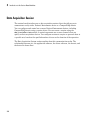
Data Acquisition System . . . . . . . . . . . . . . . . . . . . . . . . . . . . . .
Overview . . . . . . . . . . . . . . . . . . . . . . . . . . . . . . . . . . . . . . . .
Data Acquisition Hardware . . . . . . . . . . . . . . . . . . . . . . . . .
Sensors . . . . . . . . . . . . . . . . . . . . . . . . . . . . . . . . . . . . . . . .
Signal Conditioning . . . . . . . . . . . . . . . . . . . . . . . . . . . . . . .
The Computer . . . . . . . . . . . . . . . . . . . . . . . . . . . . . . . . . . .
Software . . . . . . . . . . . . . . . . . . . . . . . . . . . . . . . . . . . . . . .
1-8
1-8
1-10
1-12
1-15
1-17
1-17
Analog Input Subsystem . . . . . . . . . . . . . . . . . . . . . . . . . . . . .
Function of the Analog Input Subsystem . . . . . . . . . . . . . . .
Sampling . . . . . . . . . . . . . . . . . . . . . . . . . . . . . . . . . . . . . . .
Quantization . . . . . . . . . . . . . . . . . . . . . . . . . . . . . . . . . . . .
Channel Configuration . . . . . . . . . . . . . . . . . . . . . . . . . . . .
Transferring Data from Hardware to System Memory . . . . .
1-20
1-20
1-21
1-23
1-27
1-29
Making Quality Measurements . . . . . . . . . . . . . . . . . . . . . . .
What Do You Measure? . . . . . . . . . . . . . . . . . . . . . . . . . . . .
Accuracy and Precision . . . . . . . . . . . . . . . . . . . . . . . . . . . .
Noise . . . . . . . . . . . . . . . . . . . . . . . . . . . . . . . . . . . . . . . . . .
1-32
1-32
1-32
1-36
v
2
vi
Contents
Matching the Sensor Range and A/D Converter Range . . . .
How Fast Should a Signal Be Sampled? . . . . . . . . . . . . . . .
1-37
1-37
Getting Command-Line Function Help . . . . . . . . . . . . . . . . .
1-41
Selected Bibliography . . . . . . . . . . . . . . . . . . . . . . . . . . . . . . .
1-42
Using Data Acquisition Toolbox Software
Installation Information . . . . . . . . . . . . . . . . . . . . . . . . . . . . . .
Prerequisites . . . . . . . . . . . . . . . . . . . . . . . . . . . . . . . . . . . . .
Toolbox Installation . . . . . . . . . . . . . . . . . . . . . . . . . . . . . . . .
Hardware and Driver Installation . . . . . . . . . . . . . . . . . . . . .
2-2
2-2
2-2
2-3
Toolbox Components . . . . . . . . . . . . . . . . . . . . . . . . . . . . . . . . .
Information and Interaction . . . . . . . . . . . . . . . . . . . . . . . . .
MATLAB Functions . . . . . . . . . . . . . . . . . . . . . . . . . . . . . . .
Data Acquisition Engine . . . . . . . . . . . . . . . . . . . . . . . . . . . .
Hardware Driver Adaptor . . . . . . . . . . . . . . . . . . . . . . . . . . .
Supported Hardware . . . . . . . . . . . . . . . . . . . . . . . . . . . . . . .
Unsupported Hardware . . . . . . . . . . . . . . . . . . . . . . . . . . . .
2-4
2-4
2-6
2-6
2-9
2-9
2-11
Accessing Your Hardware . . . . . . . . . . . . . . . . . . . . . . . . . . .
Connecting to Your Hardware . . . . . . . . . . . . . . . . . . . . . . .
Acquiring Data . . . . . . . . . . . . . . . . . . . . . . . . . . . . . . . . . .
Outputting Data . . . . . . . . . . . . . . . . . . . . . . . . . . . . . . . . .
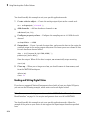
Reading and Writing Digital Values . . . . . . . . . . . . . . . . . .
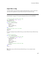
Acquire Data in a Loop . . . . . . . . . . . . . . . . . . . . . . . . . . . .
2-12
2-12
2-12
2-13
2-14
2-17
Understanding the Toolbox Capabilities . . . . . . . . . . . . . . .
Contents File . . . . . . . . . . . . . . . . . . . . . . . . . . . . . . . . . . . .
Documentation Examples . . . . . . . . . . . . . . . . . . . . . . . . . .
Examples . . . . . . . . . . . . . . . . . . . . . . . . . . . . . . . . . . . . . . .
2-19
2-19
2-19
2-20
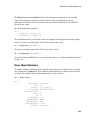
Examine Your Hardware Resources . . . . . . . . . . . . . . . . . . .
Using the daqhwinfo Function . . . . . . . . . . . . . . . . . . . . . .
General Toolbox Information . . . . . . . . . . . . . . . . . . . . . . . .
Adaptor-Specific Information . . . . . . . . . . . . . . . . . . . . . . . .
Device Object Information . . . . . . . . . . . . . . . . . . . . . . . . . .
2-21
2-21
2-21
2-22
2-23
Getting Help . . . . . . . . . . . . . . . . . . . . . . . . . . . . . . . . . . . . . . .
The daqhelp Function . . . . . . . . . . . . . . . . . . . . . . . . . . . . .
The propinfo Function . . . . . . . . . . . . . . . . . . . . . . . . . . . . .
3
4
2-25
2-25
2-25
Introduction to the Session-Based Interface
Data Acquisition Session . . . . . . . . . . . . . . . . . . . . . . . . . . . . .
3-2
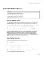
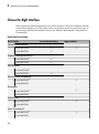
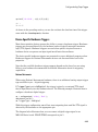
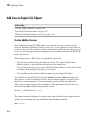
Choose the Right Interface . . . . . . . . . . . . . . . . . . . . . . . . . . .
3-4
Getting Help . . . . . . . . . . . . . . . . . . . . . . . . . . . . . . . . . . . . . . . .
Command-Line Help . . . . . . . . . . . . . . . . . . . . . . . . . . . . . . .
Online Help . . . . . . . . . . . . . . . . . . . . . . . . . . . . . . . . . . . . . .
Session-Based Interface Examples . . . . . . . . . . . . . . . . . . . .
3-7
3-7
3-7
3-7
Data Acquisition Workflow
Understanding the Data Acquisition Workflow . . . . . . . . . . .
Overview . . . . . . . . . . . . . . . . . . . . . . . . . . . . . . . . . . . . . . . .
Real-Time Data Acquisition . . . . . . . . . . . . . . . . . . . . . . . . .
Data Acquisition Workflow . . . . . . . . . . . . . . . . . . . . . . . . . .
4-2
4-2
4-3
4-4
Create a Device Object . . . . . . . . . . . . . . . . . . . . . . . . . . . . . . .
Understanding Device Objects . . . . . . . . . . . . . . . . . . . . . . .
Create an Array of Device Objects . . . . . . . . . . . . . . . . . . . .
Where Do Device Objects Exist? . . . . . . . . . . . . . . . . . . . . . .
4-6
4-6
4-7
4-8
Hardware Channels or Lines . . . . . . . . . . . . . . . . . . . . . . . . .
Add Channels and Lines . . . . . . . . . . . . . . . . . . . . . . . . . . .
Hardware Channel IDs to the MATLAB Indices . . . . . . . . .
4-10
4-10
4-11
Configure and Return Properties . . . . . . . . . . . . . . . . . . . . .
Overview . . . . . . . . . . . . . . . . . . . . . . . . . . . . . . . . . . . . . . .
Property Types . . . . . . . . . . . . . . . . . . . . . . . . . . . . . . . . . .
Return Property Names and Property Values . . . . . . . . . . .
4-14
4-14
4-14
4-16
vii
5
6
viii
Contents
Configure Property Values . . . . . . . . . . . . . . . . . . . . . . . . .
Specify Property Names . . . . . . . . . . . . . . . . . . . . . . . . . . .
Default Property Values . . . . . . . . . . . . . . . . . . . . . . . . . . .
Property Inspector . . . . . . . . . . . . . . . . . . . . . . . . . . . . . . . .
4-17
4-17
4-18
4-18
Acquire and Output Data . . . . . . . . . . . . . . . . . . . . . . . . . . . .
Device Object States . . . . . . . . . . . . . . . . . . . . . . . . . . . . . .
Start the Device Object . . . . . . . . . . . . . . . . . . . . . . . . . . . .
Log or Send Data . . . . . . . . . . . . . . . . . . . . . . . . . . . . . . . .
Stop the Device Object . . . . . . . . . . . . . . . . . . . . . . . . . . . .
4-20
4-20
4-21
4-21
4-22
Clean Up . . . . . . . . . . . . . . . . . . . . . . . . . . . . . . . . . . . . . . . . . .
4-24
Session-Based Interface Workflows
Session Creation Workflow . . . . . . . . . . . . . . . . . . . . . . . . . . .
5-2
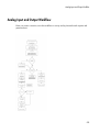
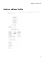
Analog Input and Output Workflow . . . . . . . . . . . . . . . . . . . .
5-5
Digital Input and Output Workflow . . . . . . . . . . . . . . . . . . . .
5-7
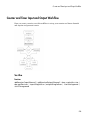
Counter and Timer Input and Output Workflow . . . . . . . . . .
5-9
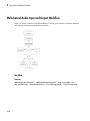
Multichannel Audio Input and Output Workflow . . . . . . . .
5-10
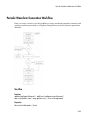
Periodic Waveform Generation Workflow . . . . . . . . . . . . . .
5-11
Getting Started with Analog Input
Create an Analog Input Object . . . . . . . . . . . . . . . . . . . . . . . .
6-2
Add Channels to an Analog Input Object . . . . . . . . . . . . . . . .
Channel Group . . . . . . . . . . . . . . . . . . . . . . . . . . . . . . . . . . .
Reference Individual Hardware Channels . . . . . . . . . . . . . . .
Add Channels for a Sound Card . . . . . . . . . . . . . . . . . . . . . .
6-4
6-4
6-5
6-7
7
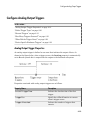
Configure Analog Input Properties . . . . . . . . . . . . . . . . . . . . .
Analog Input: Basic Properties . . . . . . . . . . . . . . . . . . . . . . .
Sampling Rate . . . . . . . . . . . . . . . . . . . . . . . . . . . . . . . . . . . .
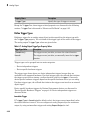
Trigger Types . . . . . . . . . . . . . . . . . . . . . . . . . . . . . . . . . . .
Samples to Acquire per Trigger . . . . . . . . . . . . . . . . . . . . . .
6-9
6-9
6-9
6-11
6-12
Acquire Data . . . . . . . . . . . . . . . . . . . . . . . . . . . . . . . . . . . . . . .
Start Analog Input Object . . . . . . . . . . . . . . . . . . . . . . . . . .
Log Data . . . . . . . . . . . . . . . . . . . . . . . . . . . . . . . . . . . . . . .
Stop Analog Input Object . . . . . . . . . . . . . . . . . . . . . . . . . .
6-14
6-14
6-14
6-15
Analog Input Examples . . . . . . . . . . . . . . . . . . . . . . . . . . . . . .
Basic Steps for Acquiring Data . . . . . . . . . . . . . . . . . . . . . .
Acquire Data with a Sound Card . . . . . . . . . . . . . . . . . . . .
Acquire Data with a National Instruments Board . . . . . . . .
6-16
6-16
6-16
6-20
Evaluate Analog Input Object Status . . . . . . . . . . . . . . . . . .
Status Properties . . . . . . . . . . . . . . . . . . . . . . . . . . . . . . . . .
Display Summary . . . . . . . . . . . . . . . . . . . . . . . . . . . . . . . .
6-24
6-24
6-25
Doing More with Analog Input
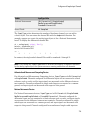
Configure and Sample Input Channels . . . . . . . . . . . . . . . . . .
Properties Associated with Configuring and Sampling Input
Channels . . . . . . . . . . . . . . . . . . . . . . . . . . . . . . . . . . . . . .
Configure Input Channel . . . . . . . . . . . . . . . . . . . . . . . . . . .
Sampling Rate . . . . . . . . . . . . . . . . . . . . . . . . . . . . . . . . . . . .
Channel Skew . . . . . . . . . . . . . . . . . . . . . . . . . . . . . . . . . . . .
7-2
Manage Acquired Data . . . . . . . . . . . . . . . . . . . . . . . . . . . . . . .
Analog Input Data Management Properties . . . . . . . . . . . . .
Preview Data . . . . . . . . . . . . . . . . . . . . . . . . . . . . . . . . . . . .
Rules for Using peekdata . . . . . . . . . . . . . . . . . . . . . . . . . .
Poll the Data Block . . . . . . . . . . . . . . . . . . . . . . . . . . . . . . .
Extract Data from the Engine . . . . . . . . . . . . . . . . . . . . . . .
Preview and Extract Data . . . . . . . . . . . . . . . . . . . . . . . . . .
Return Time Information . . . . . . . . . . . . . . . . . . . . . . . . . .
7-9
7-9
7-9
7-10
7-11
7-12
7-14
7-16
7-2
7-2
7-9
7-6
ix
8
x
Contents
Configure Analog Input Triggers . . . . . . . . . . . . . . . . . . . . .
Analog Input Trigger Properties . . . . . . . . . . . . . . . . . . . . .
Define Trigger Types and Conditions . . . . . . . . . . . . . . . . .
Execute the Trigger . . . . . . . . . . . . . . . . . . . . . . . . . . . . . . .
Trigger Delays . . . . . . . . . . . . . . . . . . . . . . . . . . . . . . . . . . .
Repeat Triggers . . . . . . . . . . . . . . . . . . . . . . . . . . . . . . . . . .
How Many Triggers Occurred? . . . . . . . . . . . . . . . . . . . . . .
When Did the Trigger Occur? . . . . . . . . . . . . . . . . . . . . . . .
Device-Specific Hardware Triggers . . . . . . . . . . . . . . . . . . .
7-19
7-19
7-20
7-25
7-25
7-28
7-33
7-34
7-35
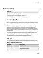
Events and Callbacks . . . . . . . . . . . . . . . . . . . . . . . . . . . . . . .
Events and Callbacks Basics . . . . . . . . . . . . . . . . . . . . . . . .
Event Types . . . . . . . . . . . . . . . . . . . . . . . . . . . . . . . . . . . .
Record and Retrieve Event Information . . . . . . . . . . . . . . .
Create and Execute Callback Functions . . . . . . . . . . . . . . .
Use Callback Properties and Functions . . . . . . . . . . . . . . . .
7-41
7-41
7-41
7-44
7-47
7-49
Scaling Data Linearly . . . . . . . . . . . . . . . . . . . . . . . . . . . . . . .
Analog Input Engineering Units Properties . . . . . . . . . . . . .
Perform Linear Conversion . . . . . . . . . . . . . . . . . . . . . . . . .
Linear Conversion with Asymmetric Data . . . . . . . . . . . . . .
7-52
7-52
7-53
7-55
Analog Output
Getting Started with Analog Output . . . . . . . . . . . . . . . . . . . .
Create an Analog Output Object . . . . . . . . . . . . . . . . . . . . . .
Add Channels to an Analog Output Object . . . . . . . . . . . . . .
Analog Output Properties . . . . . . . . . . . . . . . . . . . . . . . . . . .
Output Data . . . . . . . . . . . . . . . . . . . . . . . . . . . . . . . . . . . . .
Analog Output Examples . . . . . . . . . . . . . . . . . . . . . . . . . . .
Evaluate the Analog Output Object Status . . . . . . . . . . . . .
8-2
8-2
8-3
8-4
8-7
8-8
8-11
Manage Output Data . . . . . . . . . . . . . . . . . . . . . . . . . . . . . . . .
Analog Output Subsystem . . . . . . . . . . . . . . . . . . . . . . . . . .
Data Queuing . . . . . . . . . . . . . . . . . . . . . . . . . . . . . . . . . . .
Queue Data with putdata . . . . . . . . . . . . . . . . . . . . . . . . . .
8-15
8-15
8-15
8-17
Configure Analog Output Triggers . . . . . . . . . . . . . . . . . . . .
Analog Output Trigger Properties . . . . . . . . . . . . . . . . . . . .
8-19
8-19
9
10
Define Trigger Types . . . . . . . . . . . . . . . . . . . . . . . . . . . . . .
Execute Triggers . . . . . . . . . . . . . . . . . . . . . . . . . . . . . . . . .
How Many Triggers Occurred? . . . . . . . . . . . . . . . . . . . . . .
When Did the Trigger Occur? . . . . . . . . . . . . . . . . . . . . . . .
Device-Specific Hardware Triggers . . . . . . . . . . . . . . . . . . .
8-20
8-21
8-21
8-22
8-23
Events and Callbacks . . . . . . . . . . . . . . . . . . . . . . . . . . . . . . .
Events and Callbacks Basics . . . . . . . . . . . . . . . . . . . . . . . .
Event Types . . . . . . . . . . . . . . . . . . . . . . . . . . . . . . . . . . . .
Record and Retrieve Event Information . . . . . . . . . . . . . . .
Use Callback Properties and Callback Functions . . . . . . . . .
8-25
8-25
8-25
8-27
8-30
Scale Data Linearly . . . . . . . . . . . . . . . . . . . . . . . . . . . . . . . . .
Engineering Units . . . . . . . . . . . . . . . . . . . . . . . . . . . . . . . .
Perform a Linear Conversion . . . . . . . . . . . . . . . . . . . . . . .
8-33
8-33
8-34
Start Multiple Device Objects . . . . . . . . . . . . . . . . . . . . . . . .
8-36
Advanced Configurations Using Analog Input and
Analog Output
Start Analog Input and Output Simultaneously . . . . . . . . . .
9-2
Synchronize Analog Input and Output Using RTSI . . . . . . .
9-4
Digital Input/Output
Digital I/O Subsystems . . . . . . . . . . . . . . . . . . . . . . . . . . . . . .
10-2
Digital I/O Objects . . . . . . . . . . . . . . . . . . . . . . . . . . . . . . . . . .
Create a Digital I/O Object . . . . . . . . . . . . . . . . . . . . . . . . .
Parallel Port . . . . . . . . . . . . . . . . . . . . . . . . . . . . . . . . . . . .
10-3
10-3
10-4
Add Lines to Digital I/O Objects . . . . . . . . . . . . . . . . . . . . . .
Use the Addline Function . . . . . . . . . . . . . . . . . . . . . . . . . .
10-6
10-6
xi
Line and Port Characteristics . . . . . . . . . . . . . . . . . . . . . . .
Reference Individual Hardware Lines . . . . . . . . . . . . . . . .
11
12
Write and Read Digital I/O Line Values . . . . . . . . . . . . . . .
Write Digital Values . . . . . . . . . . . . . . . . . . . . . . . . . . . . .
Read Digital Values . . . . . . . . . . . . . . . . . . . . . . . . . . . . .
Write and Read Digital Values . . . . . . . . . . . . . . . . . . . . .
10-14
10-14
10-16
10-17
Generate Timer Events . . . . . . . . . . . . . . . . . . . . . . . . . . . . .
Overview . . . . . . . . . . . . . . . . . . . . . . . . . . . . . . . . . . . . . .
Timer Events . . . . . . . . . . . . . . . . . . . . . . . . . . . . . . . . . . .
Start and Stop a Digital I/O Object . . . . . . . . . . . . . . . . . .
Generate Timer Events . . . . . . . . . . . . . . . . . . . . . . . . . . .
10-19
10-19
10-19
10-20
10-20
Evaluate Digital I/O Object Status . . . . . . . . . . . . . . . . . . .
Running Property . . . . . . . . . . . . . . . . . . . . . . . . . . . . . . .
Display Summary . . . . . . . . . . . . . . . . . . . . . . . . . . . . . . .
10-22
10-22
10-22
Saving and Loading
Save and Load Device Objects . . . . . . . . . . . . . . . . . . . . . . . .
Save Device Objects to a File . . . . . . . . . . . . . . . . . . . . . . .
Save Device Objects to a MAT-File . . . . . . . . . . . . . . . . . . .
11-2
11-2
11-3
Log Information to Disk . . . . . . . . . . . . . . . . . . . . . . . . . . . . .
Analog Input Logging Properties . . . . . . . . . . . . . . . . . . . . .
Specify a Filename . . . . . . . . . . . . . . . . . . . . . . . . . . . . . . .
Retrieve Logged Information . . . . . . . . . . . . . . . . . . . . . . . .
Log and Retrieve Information . . . . . . . . . . . . . . . . . . . . . . .
11-5
11-5
11-6
11-7
11-9
softscope: The Data Acquisition Oscilloscope
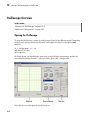
Oscilloscope Overview . . . . . . . . . . . . . . . . . . . . . . . . . . . . . .
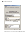
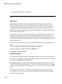
Opening the Oscilloscope . . . . . . . . . . . . . . . . . . . . . . . . . . .
Hardware Configuration . . . . . . . . . . . . . . . . . . . . . . . . . . .
xii
Contents
10-7
10-11
12-2
12-2
12-3
13
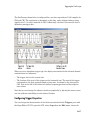
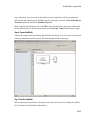
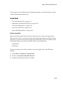
Displaying Channels . . . . . . . . . . . . . . . . . . . . . . . . . . . . . . . .
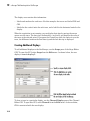
Creating a Display . . . . . . . . . . . . . . . . . . . . . . . . . . . . . . .
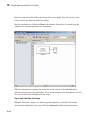
Creating Additional Displays . . . . . . . . . . . . . . . . . . . . . . .
Configuring Display Properties . . . . . . . . . . . . . . . . . . . . . .
Math and Reference Channels . . . . . . . . . . . . . . . . . . . . . .
Removing Channel Displays . . . . . . . . . . . . . . . . . . . . . . .
12-5
12-5
12-6
12-7
12-8
12-11
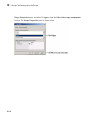
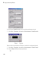
Channel Data and Properties . . . . . . . . . . . . . . . . . . . . . . . .
Scaling the Channel Data . . . . . . . . . . . . . . . . . . . . . . . . .
Configuring Channel Properties . . . . . . . . . . . . . . . . . . . .
12-13
12-13
12-14
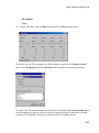
Triggering the Oscilloscope . . . . . . . . . . . . . . . . . . . . . . . . .
Acquisition Types . . . . . . . . . . . . . . . . . . . . . . . . . . . . . . .
Trigger Types . . . . . . . . . . . . . . . . . . . . . . . . . . . . . . . . . .
Configuring Trigger Properties . . . . . . . . . . . . . . . . . . . . .
12-16
12-16
12-16
12-17
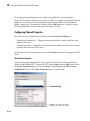
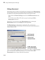
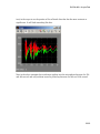
Making Measurements . . . . . . . . . . . . . . . . . . . . . . . . . . . . .
Predefined Measurement . . . . . . . . . . . . . . . . . . . . . . . . . .
Defining a Measurement . . . . . . . . . . . . . . . . . . . . . . . . . .
Defining a New Measurement Type . . . . . . . . . . . . . . . . .
Configuring Measurement Properties . . . . . . . . . . . . . . . .
12-19
12-19
12-20
12-21
12-22
Exporting Data . . . . . . . . . . . . . . . . . . . . . . . . . . . . . . . . . . . .
Channels . . . . . . . . . . . . . . . . . . . . . . . . . . . . . . . . . . . . . .
Measurements . . . . . . . . . . . . . . . . . . . . . . . . . . . . . . . . . .
12-25
12-25
12-26
Saving and Loading the Oscilloscope Configuration . . . . .
12-27
Using the Data Acquisition Blocks in Simulink
Data Acquisition Simulink Blocks Basics . . . . . . . . . . . . . . .
13-2
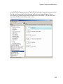
Open the Data Acquisition Block Library . . . . . . . . . . . . . .
Use the daqlib Command from the MATLAB Workspace . . .
Use the Simulink Library Browser . . . . . . . . . . . . . . . . . . .
13-3
13-3
13-4
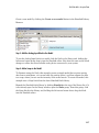
Build Models to Acquire Data . . . . . . . . . . . . . . . . . . . . . . . .
Data Acquisition Toolbox Block Library . . . . . . . . . . . . . . .
Bring Analog Data into a Model . . . . . . . . . . . . . . . . . . . . .
13-6
13-6
13-6
xiii
14
15
16
Using the Session-Based Interface
About the Session-Based Interface . . . . . . . . . . . . . . . . . . . .
Working with Sessions . . . . . . . . . . . . . . . . . . . . . . . . . . . .
Session-Based Interface and Data Acquisition Toolbox . . . .
14-2
14-2
14-4
Digital Input and Output . . . . . . . . . . . . . . . . . . . . . . . . . . . .
14-5
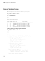
Discover Hardware Devices . . . . . . . . . . . . . . . . . . . . . . . . . .
14-6
Create a Session . . . . . . . . . . . . . . . . . . . . . . . . . . . . . . . . . . . .
14-8
Support Package Installer
Install Digilent Device Support . . . . . . . . . . . . . . . . . . . . . . .
15-2
Install Multichannel Audio Device Support . . . . . . . . . . . . .
15-4
Install National Instruments Device Support . . . . . . . . . . .
NIDAQmx Driver Requirements . . . . . . . . . . . . . . . . . . . . .
Install Support Package . . . . . . . . . . . . . . . . . . . . . . . . . . .
15-6
15-6
15-6
Session Based Analog Input and Output
Acquire Analog Input Data . . . . . . . . . . . . . . . . . . . . . . . . . .
Using addAnalogInputChannel . . . . . . . . . . . . . . . . . . . . . .
Acquire Data in the Foreground . . . . . . . . . . . . . . . . . . . . .
Acquire Data from Multiple Channels . . . . . . . . . . . . . . . . .
Acquire Data in the Background . . . . . . . . . . . . . . . . . . . . .
Acquire Data from an Accelerometer . . . . . . . . . . . . . . . . . .
Acquire Bridge Measurements . . . . . . . . . . . . . . . . . . . . . .
Acquire Sound Pressure Data . . . . . . . . . . . . . . . . . . . . . .
Acquire IEPE Data . . . . . . . . . . . . . . . . . . . . . . . . . . . . . .
xiv
Contents
16-2
16-2
16-2
16-4
16-5
16-6
16-9
16-11
16-13
Getting Started Acquiring Data with Digilent® Analog
Discovery™ . . . . . . . . . . . . . . . . . . . . . . . . . . . . . . . . . .
17
18
16-14
Generate Analog Output Signals . . . . . . . . . . . . . . . . . . . . .
Use addAnalogOutputChannel . . . . . . . . . . . . . . . . . . . . .
Generate Signals in the Foreground . . . . . . . . . . . . . . . . .
Generate Signals Using Multiple Channels . . . . . . . . . . . .
Generate Signals in the Background . . . . . . . . . . . . . . . . .
Generate Signals in the Background Continuously . . . . . .
Getting Started Generating Data with Digilent® Analog
Discovery™ . . . . . . . . . . . . . . . . . . . . . . . . . . . . . . . . . .
16-18
16-18
16-18
16-19
16-20
16-21
Acquire Data and Generate Signals Simultaneously . . . . .
16-25
16-22
Session-Based Counter Input and Output
Analog and Digital Counters . . . . . . . . . . . . . . . . . . . . . . . . .
17-2
Acquire Counter Input Data . . . . . . . . . . . . . . . . . . . . . . . . .
addCounterInputChannel . . . . . . . . . . . . . . . . . . . . . . . . . .
Acquire a Single EdgeCount . . . . . . . . . . . . . . . . . . . . . . . .
Acquire a Single Frequency Count . . . . . . . . . . . . . . . . . . .
Acquire Counter Input Data in the Foreground . . . . . . . . . .
17-3
17-3
17-3
17-4
17-5
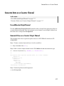
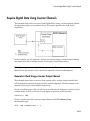
Generate Data on a Counter Channel . . . . . . . . . . . . . . . . . .
Use addCounterOutputChannel . . . . . . . . . . . . . . . . . . . . .
Generate Pulses on a Counter Output Channel . . . . . . . . . .
17-7
17-7
17-7
Session Based Digital Operations
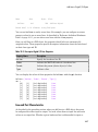
Digital Subsystem Channels . . . . . . . . . . . . . . . . . . . . . . . . . .
Digital Clocked Operations . . . . . . . . . . . . . . . . . . . . . . . . .
Access Digital Subsystem Information . . . . . . . . . . . . . . . .
18-2
18-2
18-4
Acquire Non-Clocked Digital Data . . . . . . . . . . . . . . . . . . . .
18-6
xv
19
Acquire Clocked Digital Data with Imported Clock . . . . . .
18-7
Acquire Clocked Digital Data with Shared Clock . . . . . . . .
18-9
Acquire Digital Data Using Counter Channels . . . . . . . . .
Generate a Clock Using a Counter Output Channel . . . . . .
Use Counter Clock To Acquire Clocked Digital Data . . . . .
18-11
18-11
18-12
Acquire Digital Data in Hexadecimal Values . . . . . . . . . . .
18-14
Control Stepper Motor using Digital Outputs . . . . . . . . . .
18-15
Generate Non-Clocked Digital Data . . . . . . . . . . . . . . . . . .
18-20
Generate Signals Using Decimal Data Across Multiple
Lines . . . . . . . . . . . . . . . . . . . . . . . . . . . . . . . . . . . . . . . . . .
18-21
Generate And Acquire Data On Bidirectional Channels . .
18-22
Generate Signals On Both Analog and Digital Channels .
18-24
Output Digital Data Serially Using a Software Clock . . . .
18-25
Multichannel Audio
Multichannel Audio Input and Output . . . . . . . . . . . . . . . . .
Multichannel Audio Session Rate . . . . . . . . . . . . . . . . . . . .
Multichannel Audio Range . . . . . . . . . . . . . . . . . . . . . . . . .
Acquire Multichannel Audio Data . . . . . . . . . . . . . . . . . . . .
Generate Continuous Audio Data . . . . . . . . . . . . . . . . . . . .
20
Waveform Function Generation
Digilent Analog Discovery Devices . . . . . . . . . . . . . . . . . . . .
xvi
Contents
19-2
19-2
19-2
19-3
19-4
20-2
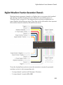
Digilent Waveform Function Generation Channels . . . . . . .
20-3
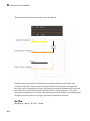
Waveform Types . . . . . . . . . . . . . . . . . . . . . . . . . . . . . . . . . . . .
20-6
Generate a Standard Waveform Using Waveform Function
Generation Channels . . . . . . . . . . . . . . . . . . . . . . . . . . . . . .
20-9
Generate an Arbitrary Waveform Using Waveform Function
Generation Channels . . . . . . . . . . . . . . . . . . . . . . . . . . . . .
20-11
21
22
Triggers and Clocks
Trigger Connections . . . . . . . . . . . . . . . . . . . . . . . . . . . . . . . .
When to Use Triggers . . . . . . . . . . . . . . . . . . . . . . . . . . . . .
External Triggering . . . . . . . . . . . . . . . . . . . . . . . . . . . . . . .
Acquire Voltage Data Using a Digital Trigger . . . . . . . . . . .
21-2
21-2
21-3
21-4
Clock Connections . . . . . . . . . . . . . . . . . . . . . . . . . . . . . . . . . .
When to Use Clocks . . . . . . . . . . . . . . . . . . . . . . . . . . . . . .
Import Scan Clock from External Source . . . . . . . . . . . . . . .
Export Scan Clock to External System . . . . . . . . . . . . . . . .
21-5
21-5
21-5
21-6
Session-Based Synchronization
Synchronization . . . . . . . . . . . . . . . . . . . . . . . . . . . . . . . . . . . .
22-2
Source and Destination Devices . . . . . . . . . . . . . . . . . . . . . .
22-5
Automatic Synchronization . . . . . . . . . . . . . . . . . . . . . . . . . .
22-6
Multiple-Device Synchronization . . . . . . . . . . . . . . . . . . . . .
Acquire Synchronized Data Using USB Devices . . . . . . . . .
Acquire Synchronized Data Using PXI Devices . . . . . . . . . .
22-7
22-7
22-9
xvii
23
Multiple-Chassis Synchronization . . . . . . . . . . . . . . . . . . . .
Acquire Synchronized Data Using CompactDAQ Devices . .
22-11
22-11
Synchronize Chassis That Do Not Support Built In
Triggers . . . . . . . . . . . . . . . . . . . . . . . . . . . . . . . . . . . . . . . .
22-12
Synchronize DSA Devices . . . . . . . . . . . . . . . . . . . . . . . . . . .
PXI DSA Devices . . . . . . . . . . . . . . . . . . . . . . . . . . . . . . . .
Hardware Restrictions . . . . . . . . . . . . . . . . . . . . . . . . . . . .
Synchronize Dynamic Signal Analyzer PXI Devices . . . . . .
PCI DSA Devices . . . . . . . . . . . . . . . . . . . . . . . . . . . . . . . .
Synchronize DSA PCI Devices . . . . . . . . . . . . . . . . . . . . . .
Handle Filter Delays with DSA Devices . . . . . . . . . . . . . .
22-13
22-13
22-13
22-16
22-17
22-17
22-18
Transition Your Code to Session-Based Interface
Transition Your Code to Session-Based Interface . . . . . . . .
Transition Common Workflow Commands . . . . . . . . . . . . . .
Acquire Analog Data . . . . . . . . . . . . . . . . . . . . . . . . . . . . . .
Use Triggers . . . . . . . . . . . . . . . . . . . . . . . . . . . . . . . . . . . .
Log Data . . . . . . . . . . . . . . . . . . . . . . . . . . . . . . . . . . . . . . .
Set Range of Analog Input Subsystem . . . . . . . . . . . . . . . . .
Fire an Event When Number of Scans Exceed Specified
Value . . . . . . . . . . . . . . . . . . . . . . . . . . . . . . . . . . . . . . . .
Use Timeout to Block MATLAB While an Operation
Completes . . . . . . . . . . . . . . . . . . . . . . . . . . . . . . . . . . . .
Count Pulses . . . . . . . . . . . . . . . . . . . . . . . . . . . . . . . . . . .
A
xviii
Contents
23-2
23-2
23-3
23-4
23-6
23-7
23-8
23-9
23-10
Troubleshooting Your Hardware
Supported Hardware . . . . . . . . . . . . . . . . . . . . . . . . . . . . . . . .
A-2
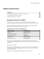
Hardware and Device Drivers . . . . . . . . . . . . . . . . . . . . . . . . .
Registering the Hardware Driver Adaptor . . . . . . . . . . . . . .
Device Driver Registration . . . . . . . . . . . . . . . . . . . . . . . . . .
A-3
A-3
A-4
Hardware Diagnostics . . . . . . . . . . . . . . . . . . . . . . . . . . . . .
Session-Based Interface Using National Instruments
Devices . . . . . . . . . . . . . . . . . . . . . . . . . . . . . . . . . . . . . . . . . .
Session-Based Interface and Legacy Interface . . . . . . . . . . .
Is My NI-DAQ Driver Supported . . . . . . . . . . . . . . . . . . . . .
Why Doesn’t My Hardware Work? . . . . . . . . . . . . . . . . . . . .
Cannot Create Session . . . . . . . . . . . . . . . . . . . . . . . . . . . . .
Why Was My Session was Deleted? . . . . . . . . . . . . . . . . . . .
Cannot Find Hardware Vendor . . . . . . . . . . . . . . . . . . . . . .
Cannot Find Devices . . . . . . . . . . . . . . . . . . . . . . . . . . . . . .
What Is a Reserved Hardware Error? . . . . . . . . . . . . . . . . .
What Are Devices with an Asterisk (*)? . . . . . . . . . . . . . . .
Network Devices Appears with an Asterisk (*) . . . . . . . . . .
ADC Overrun Error with External Clock . . . . . . . . . . . . . .
Cannot Add Clock Connection to PXI Devices . . . . . . . . . . .
Cannot Complete Long Foreground Acquisition . . . . . . . . .
Cannot Use PXI 4461 and 4462 Together . . . . . . . . . . . . . .
Counters Restart When You Call Prepare . . . . . . . . . . . . . .
Cannot Get Correct Scan Rate with Digilent Devices . . . . .
Cannot Simultaneously Acquire and Generate with myDAQ
Devices . . . . . . . . . . . . . . . . . . . . . . . . . . . . . . . . . . . . . .
Counter Single Scan Returns NaN . . . . . . . . . . . . . . . . . . .
External Clock Will Not Trigger Scan . . . . . . . . . . . . . . . . .
Why Does My S/PDIF Device Timeout? . . . . . . . . . . . . . . .
Audio Output Channels Display Incorrect
ScansOutputByHardware Value . . . . . . . . . . . . . . . . . . .
Simultaneous Analog Input and Output Not Synchronized
Correctly . . . . . . . . . . . . . . . . . . . . . . . . . . . . . . . . . . . . .
MOTU Device Not Working Correctly . . . . . . . . . . . . . . . . .
A-4
A-5
A-5
A-6
A-7
A-8
A-8
A-8
A-9
A-11
A-11
A-12
A-12
A-13
A-13
A-13
A-13
A-13
A-13
A-14
A-14
A-14
A-14
A-14
A-15
Legacy Interface Using All Devices . . . . . . . . . . . . . . . . . . .
Installed Adaptors . . . . . . . . . . . . . . . . . . . . . . . . . . . . . . .
Advantech Hardware . . . . . . . . . . . . . . . . . . . . . . . . . . . . .
Measurement Computing Hardware . . . . . . . . . . . . . . . . . .
Sound Cards . . . . . . . . . . . . . . . . . . . . . . . . . . . . . . . . . . . .
Other Manufacturers . . . . . . . . . . . . . . . . . . . . . . . . . . . . .
A-16
A-16
A-16
A-17
A-19
A-25
Contacting MathWorks . . . . . . . . . . . . . . . . . . . . . . . . . . . . . .
A-26
xix
B
C
Hardware Limitations by Vendor
National Instruments Hardware . . . . . . . . . . . . . . . . . . . . . . .
B-2
Digilent Analog Discovery Devices . . . . . . . . . . . . . . . . . . . . .
B-4
Measurement Computing Hardware . . . . . . . . . . . . . . . . . . .
B-5
Windows Sound Cards . . . . . . . . . . . . . . . . . . . . . . . . . . . . . . .
B-6
Managing Your Memory Resources
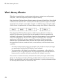
What is Memory Allocation . . . . . . . . . . . . . . . . . . . . . . . . . . .
C-2
How Much Memory Do You Need? . . . . . . . . . . . . . . . . . . . . .
C-4
Using Allocated Memory . . . . . . . . . . . . . . . . . . . . . . . . . . . . .
C-5
Glossary
xx
Contents
1
Introduction to Data Acquisition
• “Data Acquisition Toolbox Product Description” on page 1-2
• “Product Capabilities” on page 1-3
• “Anatomy of a Data Acquisition Experiment” on page 1-6
• “Data Acquisition System” on page 1-8
• “Analog Input Subsystem” on page 1-20
• “Making Quality Measurements” on page 1-32
• “Getting Command-Line Function Help” on page 1-41
• “Selected Bibliography” on page 1-42
1
Introduction to Data Acquisition
Data Acquisition Toolbox Product Description
Connect to data acquisition cards, devices, and modules
Data Acquisition Toolbox™ provides functions for connecting MATLAB® to data
acquisition hardware. The toolbox supports a variety of DAQ hardware, including
USB, PCI, PCI Express®, PXI, and PXI-Express devices, from National Instruments,
Measurement Computing, Advantech, Data Translation, and other vendors.
With the toolbox you can configure data acquisition hardware and read data into
MATLAB and Simulink® for immediate analysis. You can also send out data over analog
and digital output channels provided by data acquisition hardware. The toolbox’s data
acquisition software includes functions for controlling analog input, analog output,
counter/timer, and digital I/O subsystems of a DAQ device. You can access device-specific
features and synchronize data acquired from multiple devices.
You can analyze data as you acquire it or save it for post-processing. You can also
automate tests and make iterative updates to your test setup based on analysis results.
Simulink blocks included in the toolbox let you stream live data directly into Simulink
models, enabling you to verify and validate your models against live measured data as
part of your design verification process.
Key Features
• Support for a variety of industry-standard data acquisition boards and USB modules
• Support for analog input, analog output, counters, timers, and digital I/O
• Direct access to voltage, current, IEPE accelerometer, and thermocouple
measurements
• Live acquisition of measured data directly into MATLAB or Simulink
• Hardware and software triggers for control of data acquisition
• Device-independent software interface
1-2
Product Capabilities
Product Capabilities
In this section...
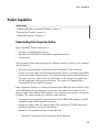
“Understanding Data Acquisition Toolbox ” on page 1-3
“Exploring the Toolbox” on page 1-4
“Supported Hardware” on page 1-5
Understanding Data Acquisition Toolbox
Data Acquisition Toolbox enables you to:
• Configure external hardware devices.
• Read data into MATLAB and Simulink for immediate analysis.
• Send out data.
You can perform these operations using two different interfaces, based on your hardware
and the platform:
• The session-based interface, which works on both Windows® 32-bit and 64-bit
systems, and only works with National Instruments® devices, including CompactDAQ
chassis and Counter/Timer modules. You cannot use other devices with this interface.
• The legacy interface, which works only on Windows 32-bit systems, and works with
all other supported data acquisition hardware. You cannot use CompactDAQ or
Counter/timer devices with this interface.
Data Acquisition Toolbox is a collection of functions and a MEX-file (shared library) built
on the MATLAB technical computing environment. The toolbox also includes several
dynamic link libraries (DLLs) called adaptors, which enable you to interface with specific
hardware. The toolbox provides you with these main features:
• A framework for bringing live, measured data into the MATLAB workspace using PCcompatible, plug-in data acquisition hardware
• Support for analog input (AI), analog output (AO), and digital I/O (DIO) subsystems
including simultaneous analog I/O conversions
• Support for these popular hardware vendors/devices:
• Advantech® boards that use the Advantech Device Manager
1-3
1
Introduction to Data Acquisition
• Measurement Computing™ Corporation (ComputerBoards) boards
• National Instruments CompactDAQ chassis using the session-based interface
• National Instruments boards that use Traditional NI-DAQ or NI-DAQmx software
Note: The Traditional NI-DAQ adaptor will not be supported in a future version of
the toolbox. If you create a Data Acquisition Toolbox™ object for Traditional NIDAQ adaptor beginning in R2008b, you will receive a warning stating that this
adaptor will be removed in a future release. See the supported hardware page at
www.mathworks.com/products/daq/supportedio.html for more information.
• Parallel ports LPT1-LPT3
Note: The parallel port adaptor will be deprecated in a future version of the
toolbox. If you create a Data Acquisition Toolbox™ object for 'parallel'
beginning in R2008b, you will receive a warning stating that this adaptor
will be removed in a future release. See the supported hardware page at
www.mathworks.com/products/daq/supportedio.html for more information.
• Microsoft® Windows sound cards
Additionally, you can use the Data Acquisition Toolbox Adaptor Kit to interface
unsupported hardware devices to the toolbox.
• Event-driven acquisitions
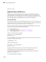
Exploring the Toolbox
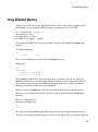
A list of the toolbox functions is available to you by typing
help daq
A list of session-based functions is available to you by typing
help sessionbasedinterface
You can view the code for any function by typing
type function_name
You can view the help for any function by typing
1-4
Product Capabilities
help function_name
You can view the help for any session-based function by typing
help daq.Session.function_name
You can change the way any toolbox function works by copying and renaming the file,
then modifying your copy. You can also extend the toolbox by adding your own files, or
by using it in combination with other products such as Signal Processing Toolbox™ or
Instrument Control Toolbox™.
MathWorks provides several related products that are especially relevant to the kinds of
tasks you can perform with Data Acquisition Toolbox. For more information about any of
these products, see http://www.mathworks.com/products/daq/related.jsp.
For more information about using National Instruments and CompactDAQ devices, see
session-based categories.
Supported Hardware
The list of hardware supported by Data Acquisition Toolbox can change in each release,
since hardware support is frequently added. The MathWorks Web site is the best place to
check for the most up-to-date listing.
To see the full list of hardware that the toolbox supports, visit the supported hardware
page at www.mathworks.com/products/daq/supportedio.html. For more information
about unsupported hardware, see “Unsupported Hardware” on page 2-11.
1-5
1
Introduction to Data Acquisition
Anatomy of a Data Acquisition Experiment
In this section...
“System Setup” on page 1-6
“Calibration” on page 1-6
“Trials” on page 1-7
System Setup
The first step in any data acquisition experiment is to install the hardware and software.
Hardware installation consists of plugging a board into your computer or installing
modules into an external chassis. Software installation consists of loading hardware
drivers and application software onto your computer. After the hardware and software
are installed, you can attach your sensors.
Calibration
After the hardware and software are installed and the sensors are connected, the data
acquisition hardware should be calibrated. Calibration consists of providing a known
input to the system and recording the output. For many data acquisition devices,
calibration can be easily accomplished with software provided by the vendor.
1-6
Anatomy of a Data Acquisition Experiment
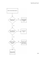
Trials
After the hardware is set up and calibrated, you can begin to acquire data. You might
think that if you completely understand the characteristics of the signal you are
measuring, then you should be able to configure your data acquisition system and
acquire the data.
In the real world however, your sensor might be picking up unacceptable noise levels and
require shielding, or you might need to run the device at a higher rate, or perhaps you
need to add an antialias filter to remove unwanted frequency components.
These real-world effects act as obstacles between you and a precise, accurate
measurement. To overcome these obstacles, you need to experiment with different
hardware and software configurations. In other words, you need to perform multiple data
acquisition trials.
1-7
1
Introduction to Data Acquisition
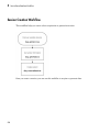
Data Acquisition System
In this section...
“Overview” on page 1-8
“Data Acquisition Hardware” on page 1-10
“Sensors” on page 1-12
“Signal Conditioning” on page 1-15
“The Computer” on page 1-17
“Software” on page 1-17
Overview
Data Acquisition Toolbox, in conjunction with the MATLAB technical computing
environment, gives you the ability to measure and analyze physical phenomena. The
purpose of any data acquisition system is to provide you with the tools and resources
necessary to do so.
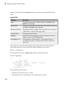
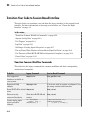
You can think of a data acquisition system as a collection of software and hardware that
connects you to the physical world. A typical data acquisition system consists of these
components.
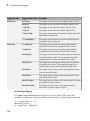
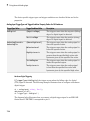
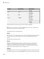
Components
Description
Data acquisition
hardware
At the heart of any data acquisition system lies the data
acquisition hardware. The main function of this hardware is to
convert analog signals to digital signals, and to convert digital
signals to analog signals.
Sensors and
actuators
(transducers)
Sensors and actuators can both be transducers. A transducer is a
device that converts input energy of one form into output energy
of another form. For example, a microphone is a sensor that
converts sound energy (in the form of pressure) into electrical
energy, while a loudspeaker is an actuator that converts
electrical energy into sound energy.
Signal conditioning Sensor signals are often incompatible with data acquisition
hardware. To overcome this incompatibility, the signal must
hardware
be conditioned. For example, you might need to condition an
input signal by amplifying it or by removing unwanted frequency
1-8
Data Acquisition System
Components
Description
components. Output signals might need conditioning as well.
However, only input signal conditioning is discussed in this
topic.
Computer
The computer provides a processor, a system clock, a bus to
transfer data, and memory and disk space to store data.
Software
Data acquisition software allows you to exchange information
between the computer and the hardware. For example, typical
software allows you to configure the sampling rate of your board,
and acquire a predefined amount of data.
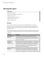
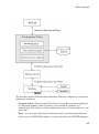
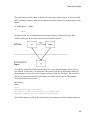
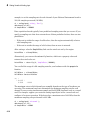
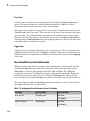
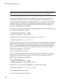
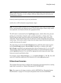
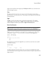
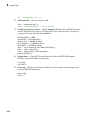
The data acquisition components, and their relationship to each other, are shown below.
The figure depicts the two important features of a data acquisition system:
• Signals are input to a sensor, conditioned, converted into bits that a computer can
read, and analyzed to extract meaningful information.
1-9
1
Introduction to Data Acquisition
For example, sound level data is acquired from a microphone, amplified, digitized by
a sound card, and stored in MATLAB workspace for subsequent analysis of frequency
content.
• Data from a computer is converted into an analog signal and output to an actuator.
For example, a vector of data in MATLAB workspace is converted to an analog signal
by a sound card and output to a loudspeaker.
Data Acquisition Hardware
Data acquisition hardware is either internal and installed directly into an expansion slot
inside your computer, or external and connected to your computer through an external
cable, which is typically a USB cable.
At the simplest level, data acquisition hardware is characterized by the subsystems it
possesses. A subsystem is a component of your data acquisition hardware that performs a
specialized task. Common subsystems include
• Analog input
• Analog output
• Digital input/output
• Counter/timer
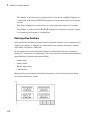
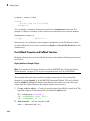
Hardware devices that consist of multiple subsystems, such as the one depicted below,
are called multifunction boards.
1-10
Data Acquisition System
Analog Input Subsystems
Analog input subsystems convert real-world analog input signals from a sensor into bits
that can be read by your computer. Perhaps the most important of all the subsystems
commonly available, they are typically multichannel devices offering 12 or 16 bits of
resolution.
Analog input subsystems are also referred to as AI subsystems, A/D converters, or ADCs.
Analog input subsystems are discussed in detail here.
Note: You cannot use the legacy interface on 64-bit MATLAB. See “About the SessionBased Interface” on page 14-2 to acquire and generate data on a 64-bit MATLAB.
Analog Output Subsystems
Analog output subsystems convert digital data stored on your computer to a realworld analog signal. These subsystems perform the inverse conversion of analog
input subsystems. Typical acquisition boards offer two output channels with 12 bits of
resolution, with special hardware available to support multiple channel analog output
operations.
Analog output subsystems are also referred to as AO subsystems, D/A converters, or
DACs.
Note: You cannot use the legacy interface on 64-bit MATLAB. See “About the SessionBased Interface” on page 14-2 to acquire and generate data on a 64-bit MATLAB.
Digital Input/Output Subsystems
Digital input/output (DIO) subsystems are designed to input and output digital values
(logic levels) to and from hardware. These values are typically handled either as single
bits or lines, or as a port, which typically consists of eight lines.
While most popular data acquisition cards include some digital I/O capability, it is
usually limited to simple operations, and special dedicated hardware is often necessary
for performing advanced digital I/O operations.
1-11
1
Introduction to Data Acquisition
Note: You cannot use the legacy interface on 64-bit MATLAB. See “About the SessionBased Interface” on page 14-2 to acquire and generate data on a 64-bit MATLAB.
Counter/Timer Subsystems
Counter/timer (C/T) subsystems are used for event counting, frequency and period
measurement, and pulse train generation. Use the session-based interface to work with
the counter/timer subsystems.
Sensors
A sensor converts the physical phenomena of interest into a signal that is input into your
data acquisition hardware. There are two main types of sensors based on the output they
produce: digital sensors and analog sensors.
Digital sensors produce an output signal that is a digital representation of the input
signal, and has discrete values of magnitude measured at discrete times. A digital sensor
must output logic levels that are compatible with the digital receiver. Some standard
logic levels include transistor-transistor logic (TTL) and emitter-coupled logic (ECL).
Examples of digital sensors include switches and position encoders.
Analog sensors produce an output signal that is directly proportional to the input
signal, and is continuous in both magnitude and in time. Most physical variables such
as temperature, pressure, and acceleration are continuous in nature and are readily
measured with an analog sensor. For example, the temperature of an automobile cooling
system and the acceleration produced by a child on a swing all vary continuously.
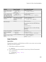
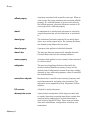
The sensor you use depends on the phenomena you are measuring. Some common analog
sensors and the physical variables they measure are listed below.
Common Analog Sensors
1-12
Sensor
Physical Variable
Accelerometer
Acceleration
Microphone
Pressure
Pressure gauge
Pressure
Resistive temperature device (RTD)
Temperature
Strain gauge
Force
Data Acquisition System
Sensor
Physical Variable
Thermocouple
Temperature
When choosing the best analog sensor to use, you must match the characteristics of the
physical variable you are measuring with the characteristics of the sensor. The two most
important sensor characteristics are:
• The sensor output
• The sensor bandwidth
Note: You can use thermocouples and accelerometers without performing linear
conversions with the session-based interface.
Sensor Output
The output from a sensor can be an analog signal or a digital signal, and the output
variable is usually a voltage although some sensors output current.
Current Signals
Current is often used to transmit signals in noisy environments because it is much less
affected by environmental noise. The full scale range of the current signal is often either
4-20 mA or 0-20 mA. A 4-20 mA signal has the advantage that even at minimum signal
value, there should be a detectable current flowing. The absence of this indicates a wiring
problem.
Before conversion by the analog input subsystem, the current signals are usually
turned into voltage signals by a current-sensing resistor. The resistor should be of
high precision, perhaps 0.03% or 0.01% depending on the resolution of your hardware.
Additionally, the voltage signal should match the signal to an input range of the analog
input hardware. For 4-20 mA signals, a 50 ohm resistor will give a voltage of 1 V for a 20
mA signal by Ohm's law.
Voltage Signals
The most commonly interfaced signal is a voltage signal. For example, thermocouples,
strain gauges, and accelerometers all produce voltage signals. There are three major
aspects of a voltage signal that you need to consider:
• Amplitude
1-13
1
Introduction to Data Acquisition
If the signal is smaller than a few millivolts, you might need to amplify it. If it is
larger than the maximum range of your analog input hardware (typically ±10 V), you
will have to divide the signal down using a resistor network.
The amplitude is related to the sensitivity (resolution) of your hardware. Refer to
Accuracy and Precision for more information about hardware sensitivity.
• Frequency
Whenever you acquire data, you should decide the highest frequency you want to
measure.
The highest frequency component of the signal determines how often you should
sample the input. If you have more than one input, but only one analog input
subsystem, then the overall sampling rate goes up in proportion to the number of
inputs. Higher frequencies might be present as noise, which you can remove by
filtering the signal before it is digitized.
If you sample the input signal at least twice as fast as the highest frequency
component, then that signal will be uniquely characterized. However, this rate might
not mimic the waveform very closely. For a rapidly varying signal, you might need
a sampling rate of roughly 10 to 20 times the highest frequency to get an accurate
picture of the waveform. For slowly varying signals, you need only consider the
minimum time for a significant change in the signal.
The frequency is related to the bandwidth of your measurement. Bandwidth is
discussed in “Sensor Bandwidth” on page 1-14.
• Duration
How long do you want to sample the signal for? If you are storing data to memory or
to a disk file, then the duration determines the storage resources required. The format
of the stored data also affects the amount of storage space required. For example, data
stored in ASCII format takes more space than data stored in binary format.
Sensor Bandwidth
In a real-world data acquisition experiment, the physical phenomena you are measuring
has expected limits. For example, the temperature of your automobile's cooling system
varies continuously between its low limit and high limit. The temperature limits, as
well as how rapidly the temperature varies between the limits, depends on several
factors including your driving habits, the weather, and the condition of the cooling
1-14
Data Acquisition System
system. The expected limits might be readily approximated, but there are an infinite
number of possible temperatures that you can measure at a given time. As explained in
Quantization, these unlimited possibilities are mapped to a finite set of values by your
data acquisition hardware.
The bandwidth is given by the range of frequencies present in the signal being measured.
You can also think of bandwidth as being related to the rate of change of the signal.
A slowly varying signal has a low bandwidth, while a rapidly varying signal has a
high bandwidth. To properly measure the physical phenomena of interest, the sensor
bandwidth must be compatible with the measurement bandwidth.
You might want to use sensors with the widest possible bandwidth when making any
physical measurement. This is the one way to ensure that the basic measurement system
is capable of responding linearly over the full range of interest. However, the wider
the bandwidth of the sensor, the more you must be concerned with eliminating sensor
response to unwanted frequency components.
Signal Conditioning
Sensor signals are often incompatible with data acquisition hardware. To overcome this
incompatibility, the sensor signal must be conditioned. The type of signal conditioning
required depends on the sensor you are using. For example, a signal might have a
small amplitude and require amplification, or it might contain unwanted frequency
components and require filtering. Common ways to condition signals include
• Amplification
• Filtering
• Electrical isolation
• Multiplexing
• Excitation source
Amplification
Low-level – less than around 100 millivolts – usually need to be amplified. High-level
signals might also require amplification depending on the input range of the analog input
subsystem.
For example, the output signal from a thermocouple is small and must be amplified
before it is digitized. Signal amplification allows you to reduce noise and to make use of
the full range of your hardware thereby increasing the resolution of the measurement.
1-15
1
Introduction to Data Acquisition
Filtering
Filtering removes unwanted noise from the signal of interest. A noise filter is used on
slowly varying signals such as temperature to attenuate higher frequency signals that
can reduce the accuracy of your measurement.
Rapidly varying signals such as vibration often require a different type of filter known as
an antialiasing filter. An antialiasing filter removes undesirable higher frequencies that
might lead to erroneous measurements.
Electrical Isolation
If the signal of interest contains high-voltage transients that could damage the computer,
then the sensor signals should be electrically isolated from the computer for safety
purposes.
You can also use electrical isolation to make sure that the readings from the data
acquisition hardware are not affected by differences in ground potentials. For example,
when the hardware device and the sensor signal are each referenced to ground, problems
occur if there is a potential difference between the two grounds. This difference can
lead to a ground loop, which might lead to erroneous measurements. Using electrically
isolated signal conditioning modules eliminates the ground loop and ensures that the
signals are accurately represented.
Multiplexing
A common technique for measuring several signals with a single measuring device is
multiplexing.
Signal conditioning devices for analog signals often provide multiplexing for use
with slowly changing signals such as temperature. This is in addition to any built-in
multiplexing on the DAQ board. The A/D converter samples one channel, switches to the
next channel and samples it, switches to the next channel, and so on. Because the same
A/D converter is sampling many channels, the effective sampling rate of each individual
channel is inversely proportional to the number of channels sampled.
You must take care when using multiplexers so that the switched signal has sufficient
time to settle. Refer to Noise for more information about settling time.
Excitation Source
Some sensors require an excitation source to operate. For example, strain gauges, and
resistive temperature devices (RTDs) require external voltage or current excitation.
1-16
Data Acquisition System
Signal conditioning modules for these sensors usually provide the necessary excitation.
RTD measurements are usually made with a current source that converts the variation
in resistance to a measurable voltage.
The Computer
The computer provides a processor, a system clock, a bus to transfer data, and memory
and disk space to store data.
The processor controls how fast data is accepted by the converter. The system clock
provides time information about the acquired data. Knowing that you recorded a
sensor reading is generally not enough. You also need to know when that measurement
occurred.
Data is transferred from the hardware to system memory via dynamic memory access
(DMA) or interrupts. DMA is hardware controlled and therefore extremely fast.
Interrupts might be slow because of the latency time between when a board requests
interrupt servicing and when the computer responds. The maximum acquisition rate is
also determined by the computer's bus architecture. Refer to How Are Acquired Samples
Clocked? for more information about DMA and interrupts.
Software
Regardless of the hardware you are using, you must send information to the hardware
and receive information from the hardware. You send configuration information to the
hardware such as the sampling rate, and receive information from the hardware such as
data, status messages, and error messages. You might also need to supply the hardware
with information so that you can integrate it with other hardware and with computer
resources. This information exchange is accomplished with software.
There are two kinds of software:
• Driver software
• Application software
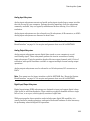
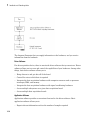
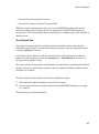
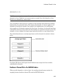
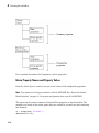
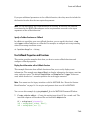
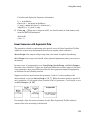
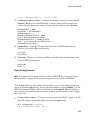
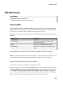
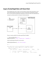
For example, suppose you are using Data Acquisition Toolbox software with a National
Instruments AT-MIO-16E-1 board and its associated NI-DAQ driver. The relationship
between you, the driver software, the application software, and the hardware is shown
below.
1-17
1
Introduction to Data Acquisition
The diagram illustrates that you supply information to the hardware, and you receive
information from the hardware.
Driver Software
For data acquisition device, there is associated driver software that you must use. Driver
software allows you to access and control the capabilities of your hardware. Among other
things, basic driver software allows you to
• Bring data on to and get data off of the board
• Control the rate at which data is acquired
• Integrate the data acquisition hardware with computer resources such as processor
interrupts, DMA, and memory
• Integrate the data acquisition hardware with signal conditioning hardware
• Access multiple subsystems on a given data acquisition board
• Access multiple data acquisition boards
Application Software
Application software provides a convenient front end to the driver software. Basic
application software allows you to
• Report relevant information such as the number of samples acquired
1-18
Data Acquisition System
• Generate events
• Manage the data stored in computer memory
• Condition a signal
• Plot acquired data
With some application software, you can also perform analysis on the data. MATLAB and
Data Acquisition Toolbox software provide you with these capabilities and more.
1-19
1
Introduction to Data Acquisition
Analog Input Subsystem
In this section...
“Function of the Analog Input Subsystem” on page 1-20
“Sampling” on page 1-21
“Quantization” on page 1-23
“Channel Configuration” on page 1-27
“Transferring Data from Hardware to System Memory” on page 1-29
Function of the Analog Input Subsystem
Note: You cannot use the legacy interface on 64-bit MATLAB. See “About the SessionBased Interface” on page 14-2 to acquire and generate data on a 64-bit MATLAB.
Many data acquisition hardware devices contain one or more subsystems that convert
(digitize) real-world sensor signals into numbers your computer can read. Such devices
are called analog input subsystems (AI subsystems, A/D converters, or ADCs). After the
real-world signal is digitized, you can analyze it, store it in system memory, or store it to
a disk file.
The function of the analog input subsystem is to sample and quantize the analog signal
using one or more channels. You can think of a channel as a path through which the
sensor signal travels. Typical analog input subsystems have eight or 16 input channels
available to you. After data is sampled and quantized, it must be transferred to system
memory.
Analog signals are continuous in time and in amplitude (within predefined limits).
Sampling takes a “snapshot” of the signal at discrete times, while quantization divides
the voltage (or current) value into discrete amplitudes. Sampling, quantization, channel
configuration, and transferring data from hardware to system memory are discussed
next.
1-20
Analog Input Subsystem
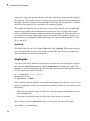
Sampling
Sampling takes a snapshot of the sensor signal at discrete times. For most applications,
the time interval between samples is kept constant (for example, sample every
millisecond) unless externally clocked.
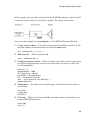
For most digital converters, sampling is performed by a sample and hold (S/H) circuit. An
S/H circuit usually consists of a signal buffer followed by an electronic switch connected
to a capacitor. The operation of an S/H circuit follows these steps:
1
At a given sampling instant, the switch connects the buffer and capacitor to an
input.
2
The capacitor is charged to the input voltage.
3
The charge is held until the A/D converter digitizes the signal.
4
For multiple channels connected (multiplexed) to one A/D converter, the previous
steps are repeated for each input channel.
5
The entire process is repeated for the next sampling instant.
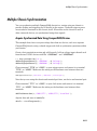
A multiplexer, S/H circuit, and A/D converter are illustrated in the next section.
Hardware can be divided into two main categories based on how signals are sampled:
scanning hardware, which samples input signals sequentially, and simultaneous sample
and hold (SS/H) hardware, which samples all signals at the same time. These two types
of hardware are discussed below.
Scanning Hardware
Scanning hardware samples a single input signal, converts that signal to a digital value,
and then repeats the process for every input channel used. In other words, each input
channel is sampled sequentially. A scan occurs when each input in a group is sampled
once.
As shown below, most data acquisition devices have one A/D converter that is
multiplexed to multiple input channels.
1-21
1
Introduction to Data Acquisition
Therefore, if you use multiple channels, those channels cannot be sampled
simultaneously and a time gap exists between consecutive sampled channels. This time
gap is called the channel skew. You can think of the channel skew as the time it takes the
analog input subsystem to sample a single channel.
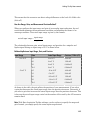
Additionally, the maximum sampling rate your hardware is rated at typically applies for
one channel. Therefore, the maximum sampling rate per channel is given by the formula:
maximum sampling rate per channel =
maximum board rate
number of channels scanned
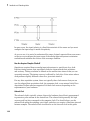
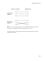
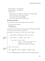
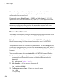
Typically, you can achieve this maximum rate only under ideal conditions. In practice,
the sampling rate depends on several characteristics of the analog input subsystem
including the settling time and the gain, as well as the channel skew. The sample period
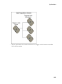
and channel skew for a multichannel configuration using scanning hardware is shown
below.
1-22
Analog Input Subsystem
If you cannot tolerate channel skew in your application, you must use hardware that
allows simultaneous sampling of all channels. Simultaneous sample and hold hardware
is discussed in the next section.
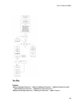
Simultaneous Sample and Hold Hardware
Simultaneous sample and hold (SS/H) hardware samples all input signals at the same
time and holds the values until the A/D converter digitizes all the signals. For high-end
systems, there can be a separate A/D converter for each input channel.
For example, suppose you need to simultaneously measure the acceleration of multiple
accelerometers to determine the vibration of some device under test. To do this, you must
use SS/H hardware because it does not have a channel skew. In general, you might need
to use SS/H hardware if your sensor signal changes significantly in a time that is less
than the channel skew, or if you need to use a transfer function or perform a frequency
domain correlation.
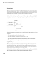
The sample period for a multichannel configuration using SS/H hardware is shown
below. Note that there is no channel skew.
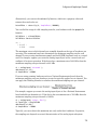
Quantization
As discussed in the previous section, sampling takes a snapshot of the input signal
at an instant of time. When the snapshot is taken, the sampled analog signal must
be converted from a voltage value to a binary number that the computer can read.
The conversion from an infinitely precise amplitude to a binary number is called
quantization.
1-23
1
Introduction to Data Acquisition
During quantization, the A/D converter uses a finite number of evenly spaced values to
represent the analog signal. The number of different values is determined by the number
of bits used for the conversion. Most modern converters use 12 or 16 bits. Typically, the
converter selects the digital value that is closest to the actual sampled value.
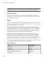
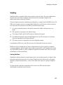
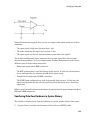
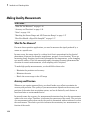
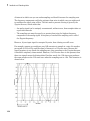
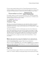
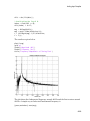
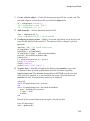
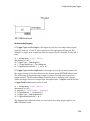
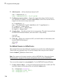
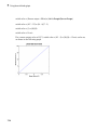
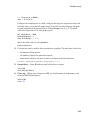
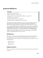
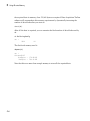
The figure below shows a 1 Hz sine wave quantized by a 3 bit A/D converter.
The number of quantized values is given by 23 = 8, the largest representable value is
given by 111 = 22 + 21 + 20 = 7.0, and the smallest representable value is given by 000 =
0.0.
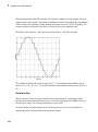
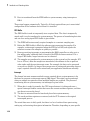
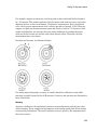
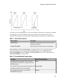
Quantization Error
There is always some error associated with the quantization of a continuous signal.
Ideally, the maximum quantization error is ±0.5 least significant bits (LSBs), and over
the full input range, the average quantization error is zero.
As shown below, the quantization error for the previous sine wave is calculated by
subtracting the actual signal from the quantized signal.
1-24
Analog Input Subsystem
Input Range and Polarity
The input range of the analog input subsystem is the span of input values for which a
conversion is valid. You can change the input range by selecting a different gain value.
For example, National Instruments' AT-MIO-16E-1 board has eight gain values ranging
from 0.5 to 100. Many boards include a programmable gain amplifier that allows you to
change the device gain through software.
When an input signal exceeds the valid input range of the converter, an overrange
condition occurs. In this case, most devices saturate to the largest representable value,
and the converted data is almost definitely incorrect. The gain setting affects the
precision of your measurement — the higher (lower) the gain value, the lower (higher)
the precision. Refer to How Are Range, Gain, and Measurement Precision Related? for
more information about how input range, gain, and precision are related to each other.
An analog input subsystem can typically convert both unipolar signals and bipolar
signals. A unipolar signal contains only positive values and zero, while a bipolar signal
contains positive values, negative values, and zero.
Unipolar and bipolar signals are depicted below. Refer to the figure in “Quantization” on
page 1-23 for an example of a unipolar signal.
1-25
1
Introduction to Data Acquisition
In many cases, the signal polarity is a fixed characteristic of the sensor and you must
configure the input range to match this polarity.
As you can see, it is crucial to understand the range of signals expected from your sensor
so that you can configure the input range of the analog input subsystem to maximize
resolution and minimize the chance of an overrange condition.
How Are Acquired Samples Clocked?
Samples are acquired from an analog input subsystem at a specific rate by a clock.
Like any timing system, data acquisition clocks are characterized their resolution
and accuracy. Timing resolution is defined as the smallest time interval that you can
accurately measure. The timing accuracy is affected by clock jitter. Jitter arises when a
clock produces slightly different values for a given time interval.
For any data acquisition system, there are typically three clock sources that you can
use: the onboard data acquisition clock, the computer clock, or an external clock. Data
Acquisition Toolbox software supports all of these clock sources, depending on the
requirements of your hardware.
Onboard Clock
The onboard clock is typically a timer chip on the hardware board that is programmed
to generate a pulse stream at the desired rate. The onboard clock generally has high
accuracy and low jitter compared to the computer clock. You should always use the
onboard clock when the sampling rate is high, and when you require a fixed time interval
between samples. The onboard clock is referred to as the internal clock in this guide.
1-26
Analog Input Subsystem
Computer Clock
The computer (PC) clock is used for boards that do not possess an onboard clock. The
computer clock is less accurate and has more jitter than the onboard clock, and is
generally limited to sampling rates below 500 Hz. The computer clock is referred to as
the software clock in this guide.
External Clock
An external clock is often used when the sampling rate is low and not constant. For
example, an external clock source is often used in automotive applications where samples
are acquired as a function of crank angle.
Channel Configuration
You can configure input channels in one of these two ways:
• Differential
• Single-ended
Your choice of input channel configuration might depend on whether the input signal is
floating or grounded.
A floating signal uses an isolated ground reference and is not connected to the building
ground. As a result, the input signal and hardware device are not connected to a common
reference, which can cause the input signal to exceed the valid range of the hardware
device. To circumvent this problem, you must connect the signal to the onboard ground
of the device. Examples of floating signal sources include ungrounded thermocouples and
battery devices.
A grounded signal is connected to the building ground. As a result, the input signal and
hardware device are connected to a common reference. Examples of grounded signal
sources include nonisolated instrument outputs and devices that are connected to the
building power system.
Note For more information about channel configuration, refer to your hardware
documentation.
1-27
1
Introduction to Data Acquisition
Differential Inputs
When you configure your hardware for differential input, there are two signal wires
associated with each input signal — one for the input signal and one for the reference
(return) signal. The measurement is the difference in voltage between the two wires,
which helps reduce noise and any voltage that is common to both wires.
As shown below, the input signal is connected to the positive amplifier socket (labeled
+) and the return signal is connected to the negative amplifier socket (labeled -). The
amplifier has a third connector that allows these signals to be referenced to ground.
National Instruments recommends that you use differential inputs under any of these
conditions:
• The input signal is low level (less than 1 volt).
• The leads connecting the signal are greater than 10 feet.
• The input signal requires a separate ground-reference point or return signal.
• The signal leads travel through a noisy environment.
Single-Ended Inputs
When you configure your hardware for single-ended input, there is one signal wire
associated with each input signal, and each input signal is connected to the same
ground. Single-ended measurements are more susceptible to noise than differential
measurements because of differences in the signal paths.
As shown below, the input signal is connected to the positive amplifier socket (labeled +)
and the ground is connected to the negative amplifier socket (labeled -).
1-28
Analog Input Subsystem
National Instruments suggests that you can use single-ended inputs under any of these
conditions:
• The input signal is high level (greater than 1 volt).
• The leads connecting the signal are less than 10 feet.
• The input signal can share a common reference point with other signals.
You should use differential input connectors for any input signal that does not meet
the preceding conditions. You can configure many National Instruments boards for two
different types of single-ended connections:
• Referenced single-ended (RSE) connection
The RSE configuration is used for floating signal sources. In this case, the hardware
device itself provides the reference ground for the input signal.
• Nonreferenced single-ended (NRSE) connection
The NRSE input configuration is used for grounded signal sources. In this case, the
input signal provides its own reference ground and the hardware device should not
supply one.
Refer to your National Instruments hardware documentation for more information about
RSE and NRSE connections.
Transferring Data from Hardware to System Memory
The transfer of acquired data from the hardware to system memory follows these steps:
1
Acquired data is stored in the hardware's first-in first-out (FIFO) buffer.
1-29
1
Introduction to Data Acquisition
2
Data is transferred from the FIFO buffer to system memory using interrupts or
DMA.
These steps happen automatically. Typically, all that's required from you is some initial
configuration of the hardware device when it is installed.
FIFO Buffer
The FIFO buffer is used to temporarily store acquired data. The data is temporarily
stored until it can be transferred to system memory. The process of transferring data into
and out of an analog input FIFO buffer is given below:
1
The FIFO buffer stores newly acquired samples at a constant sampling rate.
2
Before the FIFO buffer is filled, the software starts removing the samples. For
example, an interrupt is generated when the FIFO is half full, and signals the
software to extract the samples as quickly as possible.
3
Because servicing interrupts or programming the DMA controller can take up to a
few milliseconds, additional data is stored in the FIFO for future retrieval. For a
larger FIFO buffer, longer latencies can be tolerated.
4
The samples are transferred to system memory via the system bus (for example, PCI
bus or AT bus). After the samples are transferred, the software is free to perform
other tasks until the next interrupt occurs. For example, the data can be processed
or saved to a disk file. As long as the average rates of storing and extracting data are
equal, acquired data will not be missed and your application should run smoothly.
Interrupts
The slowest but most common method to move acquired data to system memory is for
the board to generate an interrupt request (IRQ) signal. This signal can be generated
when one sample is acquired or when multiple samples are acquired. The process of
transferring data to system memory via interrupts is given below:
1
When data is ready for transfer, the CPU stops whatever it is doing and runs a
special interrupt handler routine that saves the current machine registers, and then
sets them to access the board.
2
The data is extracted from the board and placed into system memory.
3
The saved machine registers are restored, and the CPU returns to the original
interrupted process.
The actual data move is fairly quick, but there is a lot of overhead time spent saving,
setting up, and restoring the register information. Therefore, depending on your specific
1-30
Analog Input Subsystem
system, transferring data by interrupts might not be a good choice when the sampling
rate is greater than around 5 kHz.
DMA
Direct memory access (DMA) is a system whereby samples are automatically stored in
system memory while the processor does something else. The process of transferring data
via DMA is given below:
1
When data is ready for transfer, the board directs the system DMA controller to put
it into in system memory as soon as possible.
2
As soon as the CPU is able (which is usually very quickly), it stops interacting with
the data acquisition hardware and the DMA controller moves the data directly into
memory.
3
The DMA controller gets ready for the next sample by pointing to the next open
memory location.
4
The previous steps are repeated indefinitely, with data going to each open memory
location in a continuously circulating buffer. No interaction between the CPU and
the board is needed.
Your computer supports several different DMA channels. Depending on your application,
you can use one or more of these channels, For example, simultaneous input and output
with a sound card requires one DMA channel for the input and another DMA channel for
the output.
1-31
1
Introduction to Data Acquisition
Making Quality Measurements
In this section...
“What Do You Measure?” on page 1-32
“Accuracy and Precision” on page 1-32
“Noise” on page 1-36
“Matching the Sensor Range and A/D Converter Range” on page 1-37
“How Fast Should a Signal Be Sampled?” on page 1-37
What Do You Measure?
For most data acquisition applications, you need to measure the signal produced by a
sensor at a specific rate.
In many cases, the sensor signal is a voltage level that is proportional to the physical
phenomena of interest (for example, temperature, pressure, or acceleration). If you are
measuring slowly changing (quasi-static) phenomena like temperature, a slow sampling
rate usually suffices. If you are measuring rapidly changing (dynamic) phenomena like
vibration or acoustic measurements, a fast sampling rate is required.
To make high-quality measurements, you should follow these rules:
• Maximize the precision and accuracy
• Minimize the noise
• Match the sensor range to the A/D range
Accuracy and Precision
Whenever you acquire measured data, you should make every effort to maximize its
accuracy and precision. The quality of your measurement depends on the accuracy and
precision of the entire data acquisition system, and can be limited by such factors as
board resolution or environmental noise.
In general terms, the accuracy of a measurement determines how close the measurement
comes to the true value. Therefore, it indicates the correctness of the result. The precision
of a measurement reflects how exactly the result is determined without reference to what
the result means. The relative precision indicates the uncertainty in a measurement as a
fraction of the result.
1-32
Making Quality Measurements
For example, suppose you measure a table top with a meter stick and find its length to
be 1.502 meters. This number indicates that the meter stick (and your eyes) can resolve
distances down to at least a millimeter. Under most circumstances, this is considered
to be a fairly precise measurement with a relative precision of around 1/1500. However,
suppose you perform the measurement again and obtain a result of 1.510 meters. After
careful consideration, you discover that your initial technique for reading the meter
stick was faulty because you did not read it from directly above. Therefore, the first
measurement was not accurate.
Precision and accuracy are illustrated below.
For analog input subsystems, accuracy is usually limited by calibration errors while
precision is usually limited by the A/D converter. Accuracy and precision are discussed in
more detail below.
Accuracy
Accuracy is defined as the agreement between a measured quantity and the true value
of that quantity. Every component that appears in the analog signal path affects system
accuracy and performance. The overall system accuracy is given by the component with
the worst accuracy.
1-33
1
Introduction to Data Acquisition
For data acquisition hardware, accuracy is often expressed as a percent or a fraction of
the least significant bit (LSB). Under ideal circumstances, board accuracy is typically
±0.5 LSB. Therefore, a 12 bit converter has only 11 usable bits.
Many boards include a programmable gain amplifier, which is located just before the
converter input. To prevent system accuracy from being degraded, the accuracy and
linearity of the gain must be better than that of the A/D converter. The specified accuracy
of a board is also affected by the sampling rate and the settling time of the amplifier. The
settling time is defined as the time required for the instrumentation amplifier to settle
to a specified accuracy. To maintain full accuracy, the amplifier output must settle to a
level given by the magnitude of 0.5 LSB before the next conversion, and is on the order of
several tenths of a millisecond for most boards.
Settling time is a function of sampling rate and gain value. High rate, high gain
configurations require longer settling times while low rate, low gain configurations
require shorter settling times.
Precision
The number of bits used to represent an analog signal determines the precision
(resolution) of the device. The more bits provided by your board, the more precise your
measurement will be. A high precision, high resolution device divides the input range
into more divisions thereby allowing a smaller detectable voltage value. A low precision,
low resolution device divides the input range into fewer divisions thereby increasing the
detectable voltage value.
The overall precision of your data acquisition system is usually determined by the A/
D converter, and is specified by the number of bits used to represent the analog signal.
Most boards use 12 or 16 bits. The precision of your measurement is given by:
precision = one part in 2number of
bits
The precision in volts is given by:
precision =
voltage range
2 number
of bits
For example, if you are using a 12 bit A/D converter configured for a 10 volt range, then
precision =
1-34
10 volts
212
Making Quality Measurements
This means that the converter can detect voltage differences at the level of 0.00244 volts
(2.44 mV).
How Are Range, Gain, and Measurement Precision Related?
When you configure the input range and gain of your analog input subsystem, the end
result should maximize the measurement resolution and minimize the chance of an
overrange condition. The actual input range is given by the formula:
actual input range =
input range
gain
The relationship between gain, actual input range, and precision for a unipolar and
bipolar signal having an input range of 10 V is shown below.
Relationship Between Input Range, Gain, and Precision
Input Range
0 to 10 V
-5 to 5 V
Gain
Actual Input Range
Precision (12 Bit A/D)
1.0
0 to 10 V
2.44 mV
2.0
0 to 5 V
1.22 mV
5.0
0 to 2 V
0.488 mV
10.0
0 to 1 V
0.244 mV
0.5
-10 to 10 V
4.88 mV
1.0
-5 to 5 V
2.44 mV
2.0
-2.5 to 2.5 V
1.22 mV
5.0
-1.0 to 1.0 V
0.488 mV
10.0
-0.5 to 0.5 V
0.244 mV
As shown in the table, the gain affects the precision of your measurement. If you select
a gain that decreases the actual input range, then the precision increases. Conversely, if
you select a gain that increases the actual input range, then the precision decreases. This
is because the actual input range varies but the number of bits used by the A/D converter
remains fixed.
Note With Data Acquisition Toolbox software, you do not have to specify the range and
gain. Instead, you simply specify the actual input range desired.
1-35
1
Introduction to Data Acquisition
Noise
Noise is considered to be any measurement that is not part of the phenomena of interest.
Noise can be generated within the electrical components of the input amplifier (internal
noise), or it can be added to the signal as it travels down the input wires to the amplifier
(external noise). Techniques that you can use to reduce the effects of noise are described
below.
Removing Internal Noise
Internal noise arises from thermal effects in the amplifier. Amplifiers typically generate
a few microvolts of internal noise, which limits the resolution of the signal to this level.
The amount of noise added to the signal depends on the bandwidth of the input amplifier.
To reduce internal noise, you should select an amplifier with a bandwidth that closely
matches the bandwidth of the input signal.
Removing External Noise
External noise arises from many sources. For example, many data acquisition
experiments are subject to 60 Hz noise generated by AC power circuits. This type of noise
is referred to as pick-up or hum, and appears as a sinusoidal interference signal in the
measurement circuit. Another common interference source is fluorescent lighting. These
lights generate an arc at twice the power line frequency (120 Hz).
Noise is added to the acquisition circuit from these external sources because the signal
leads act as aerials picking up environmental electrical activity. Much of this noise is
common to both signal wires. To remove most of this common-mode voltage, you should
• Configure the input channels in differential mode. Refer to Channel Configuration for
more information about channel configuration.
• Use signal wires that are twisted together rather than separate.
• Keep the signal wires as short as possible.
• Keep the signal wires as far away as possible from environmental electrical activity.
Filtering
Filtering also reduces signal noise. For many data acquisition applications, a low-pass
filter is beneficial. As the name suggests, a low-pass filter passes the lower frequency
components but attenuates the higher frequency components. The cut-off frequency of
the filter must be compatible with the frequencies present in the signal of interest and
the sampling rate used for the A/D conversion.
1-36
Making Quality Measurements
A low-pass filter that's used to prevent higher frequencies from introducing distortion
into the digitized signal is known as an antialiasing filter if the cut-off occurs at the
Nyquist frequency. That is, the filter removes frequencies greater than one-half the
sampling frequency. These filters generally have a sharper cut-off than the normal lowpass filter used to condition a signal. Antialiasing filters are specified according to the
sampling rate of the system and there must be one filter per input signal.
Matching the Sensor Range and A/D Converter Range
When sensor data is digitized by an A/D converter, you must be aware of these two
issues:
• The expected range of the data produced by your sensor. This range depends on the
physical phenomena you are measuring and the output range of the sensor.
• The range of your A/D converter. For many devices, the hardware range is specified
by the gain and polarity.
You should select the sensor and hardware ranges such that the maximum precision is
obtained, and the full dynamic range of the input signal is covered.
For example, suppose you are using a microphone with a dynamic range of 20 dB to
140 dB and an output sensitivity of 50 mV/Pa. If you are measuring street noise in your
application, then you might expect that the sound level never exceeds 80 dB, which
corresponds to a sound pressure magnitude of 200 mPa and a voltage output from the
microphone of 10 mV. Under these conditions, you should set the input range of your
data acquisition card for a maximum signal amplitude of 10 mV, or a little more.
How Fast Should a Signal Be Sampled?
Whenever a continuous signal is sampled, some information is lost. The key objective is
to sample at a rate such that the signal of interest is well characterized and the amount
of information lost is minimized.
If you sample at a rate that is too slow, then signal aliasing can occur. Aliasing can occur
for both rapidly varying signals and slowly varying signals. For example, suppose you are
measuring temperature once a minute. If your acquisition system is picking up a 60-Hz
hum from an AC power supply, then that hum will appear as constant noise level if you
are sampling at 30 Hz.
Aliasing occurs when the sampled signal contains frequency components greater than
one-half the sampling rate. The frequency components could originate from the signal
1-37
1
Introduction to Data Acquisition
of interest in which case you are undersampling and should increase the sampling rate.
The frequency components could also originate from noise in which case you might need
to condition the signal using a filter. The rule used to prevent aliasing is given by the
Nyquist theorem, which states that
• An analog signal can be uniquely reconstructed, without error, from samples taken at
equal time intervals.
• The sampling rate must be equal to or greater than twice the highest frequency
component in the analog signal. A frequency of one-half the sampling rate is called
the Nyquist frequency.
However, if your input signal is corrupted by noise, then aliasing can still occur.
For example, suppose you configure your A/D converter to sample at a rate of 4 samples
per second (4 S/s or 4 Hz), and the signal of interest is a 1 Hz sine wave. Because the
signal frequency is one-fourth the sampling rate, then according to the Nyquist theorem,
it should be completely characterized. However, if a 5 Hz sine wave is also present, then
these two signals cannot be distinguished. In other words, the 1 Hz sine wave produces
the same samples as the 5 Hz sine wave when the sampling rate is 4 S/s. This situation is
shown below.
1-38
Making Quality Measurements
In a real-world data acquisition environment, you might need to condition the signal by
filtering out the high frequency components.
Even though the samples appear to represent a sine wave with a frequency of one-fourth
the sampling rate, the actual signal could be any sine wave with a frequency of:
( n ± 0 .25 ) ¥ ( sampling rate )
where n is zero or any positive integer. For this example, the actual signal could be at a
frequency of 3 Hz, 5 Hz, 7 Hz, 9 Hz, and so on. The relationship 0.25 x (Sampling rate)
is called the alias of a signal that may be at another frequency. In other words, aliasing
occurs when one frequency assumes the identity of another frequency.
If you sample the input signal at least twice as fast as the highest frequency component,
then that signal might be uniquely characterized, but this rate would not mimic the
waveform very closely. As shown below, to get an accurate picture of the waveform, you
need a sampling rate of roughly 10 to 20 times the highest frequency.
As shown in the top figure, the low sampling rate produces a sampled signal that appears
to be a triangular waveform. As shown in the bottom figure, a higher fidelity sampled
1-39
1
Introduction to Data Acquisition
signal is produced when the sampling rate is higher. In the latter case, the sampled
signal actually looks like a sine wave.
How Can Aliasing Be Eliminated?
The primary considerations involved in antialiasing are the sampling rate of the A/D
converter and the frequencies present in the sampled data. To eliminate aliasing, you
must
• Establish the useful bandwidth of the measurement.
• Select a sensor with sufficient bandwidth.
• Select a low-pass antialiasing analog filter that can eliminate all frequencies
exceeding this bandwidth.
• Sample the data at a rate at least twice that of the filter's upper cutoff frequency.
1-40
Getting Command-Line Function Help
Getting Command-Line Function Help
To get command-line function help, you should use the daqhelp function. For example,
to get help for the addchannel function, type
help addchannel
However, Data Acquisition Toolbox software provides “overloaded” versions of several
MATLAB functions. That is, it provides toolbox-specific implementations of these
functions using the same function name. To get command-line help for an overloaded
toolbox function using the help command, you must supply one of two possible class
directories to help:
help daqdevice/function_name
help daqchild/function_name
Note that the same help information is returned regardless of the class directory
specified.
For example, Data Acquisition Toolbox software provides an overloaded version of the
delete function. To obtain help for the MATLAB version of this function, type
help delete
You can determine if a function is overloaded by examining the last section of the help.
For delete, the help contains the following overloaded versions (not all are shown):
Overloaded methods
help char/delete.m
help scribehandle/delete.m
help daqdevice/delete.m
help daqchild/delete.m
So, to obtain help on the toolbox version of this function, type
help daqdevice/delete
1-41
1
Introduction to Data Acquisition
Selected Bibliography
[1] Transducer Interfacing Handbook — A Guide to Analog Signal Conditioning, edited
by Daniel H. Sheingold; Analog Devices Inc., Norwood, MA, 1980.
[2] Bentley, John P., Principles of Measurement Systems, Second Edition; Longman
Scientific and Technical, Harlow, Essex, UK, 1988.
[3] Bevington, Philip R., Data Reduction and Error Analysis for the Physical Sciences;
McGraw-Hill, New York, NY, 1969.
[4] Carr, Joseph J., Sensors; Prompt Publications, Indianapolis, IN, 1997.
[5] The Measurement, Instrumentation, and Sensors Handbook, edited by John G.
Webster; CRC Press, Boca Raton, FL, 1999.
[6] PCI-MIO E Series User Manual, January 1997 Edition; Part Number 320945B-01,
National Instruments, Austin, TX, 1997.
1-42
2
Using Data Acquisition Toolbox
Software
This section provides the information you need to get started with Data Acquisition
Toolbox software. The sections are as follows.
• “Installation Information” on page 2-2
• “Toolbox Components” on page 2-4
• “Accessing Your Hardware” on page 2-12
• “Understanding the Toolbox Capabilities” on page 2-19
• “Examine Your Hardware Resources” on page 2-21
• “Getting Help” on page 2-25
2
Using Data Acquisition Toolbox Software
Installation Information
In this section...
“Prerequisites” on page 2-2
“Toolbox Installation” on page 2-2
“Hardware and Driver Installation” on page 2-3
Prerequisites
To acquire live, measured data into the MATLAB workspace, or to output data from the
MATLAB software, you must install these components:
• MATLAB
• Data Acquisition Toolbox
• A supported data acquisition device (the toolbox page on the MathWorks Web
site lists all supported devices at http://www.mathworks.com/products/daq/
supportedio.html)
• Software such as drivers and support libraries, as required by your data acquisition
device
Note: If you have a hardware that is not supported by Data Acquisition Toolbox, see
“Unsupported Hardware” on page 2-11.
Toolbox Installation
To determine if Data Acquisition Toolbox software is installed on your system, type
ver
at the MATLAB prompt. The MATLAB Command Window lists information about
the software versions you are running, including installed add-on products and their
version numbers. Check the list to see if Data Acquisition Toolbox product appears. For
information about installing the toolbox, see the MATLAB Installation documentation.
If you experience installation difficulties and have Web access, look for the
license manager and installation information at the MathWorks Web site (http://
www.mathworks.com).
2-2
Installation Information
Hardware and Driver Installation
Installation of your hardware device, hardware drivers, and any other device-specific
software is described in the documentation provided by your hardware vendor.
Note You need to install all necessary device-specific software provided by your hardware
vendor in addition to Data Acquisition Toolbox software.
2-3
2
Using Data Acquisition Toolbox Software
Toolbox Components
In this section...
“Information and Interaction” on page 2-4
“MATLAB Functions” on page 2-6
“Data Acquisition Engine” on page 2-6
“Hardware Driver Adaptor” on page 2-9
“Supported Hardware” on page 2-9
“Unsupported Hardware” on page 2-11
Information and Interaction
Data Acquisition Toolbox software consists of three distinct components:
• MATLAB functions
• The data acquisition engine
• The hardware driver adaptors
As shown in the figure, these components allow you to pass information between the
MATLAB workspace and your data acquisition hardware.
2-4
Toolbox Components
The preceding diagram illustrates how information flows from component to component.
Information consists of:
• Property values – You can control the behavior of your data acquisition application
by configuring property values. In general, you can think of a property as a
characteristic of the toolbox or of the hardware driver that can be manipulated to suit
your needs.
• Data – You can acquire data from a sensor connected to an analog input subsystem
and store it in the MATLAB workspace, or output data from the MATLAB workspace
2-5
2
Using Data Acquisition Toolbox Software
to an actuator connected to an analog output subsystem. Additionally you can transfer
values (1s and 0s) between the MATLAB workspace and a digital I/O subsystem.
• Events – An event occurs at a particular time after a condition is met and might
result in one or more callbacks that you specify. Events can be generated only after
you configure the associated properties. Some ways you can use events include
initiating analysis after a predetermined amount of data is acquired, or displaying a
message to the MATLAB workspace after an error occurs.
MATLAB Functions
Note: You cannot use the legacy interface on 64-bit MATLAB. See “About the SessionBased Interface” on page 14-2 to acquire and generate data on a 64-bit MATLAB.
To perform any task with your data acquisition application, you must call MATLAB
functions from the MATLAB environment. Among other things, these functions allow you
to:
• Create device objects, which provide a gateway to your hardware's capabilities and
allow you to control the behavior of your application.
• Acquire or output data.
• Configure property values.
• Evaluate your acquisition status and hardware resources.
Refer to the MATLAB Functions list in the Data Acquisition Toolbox Documentation
Center for a list of all toolbox functions. You can also display all these functions by typing
help daq
If you are using a CompactDAQ chassis or counter timers, see “Counter and Timer Input
and Output”.
Data Acquisition Engine
The data acquisition engine (or just engine) is a MEX-file (shared library that is
executable within the MATLAB software) that
• Stores the device objects and associated property values that control your data
acquisition application
2-6
Toolbox Components
• Controls the synchronization of events
• Controls the storage of acquired or queued data
While the engine performs these tasks, you can use MATLAB for other tasks such as
analyzing acquired data. In other words, the engine and the MATLAB software are
asynchronous. The relationship between acquiring data, outputting data, and data flow is
described next.
Flow of Acquired Data
Acquiring data means that data is flowing from your hardware device into the data
acquisition engine where it is temporarily stored in memory, until you explicitly extract
it using the getdata function.
If you do not extract this data, and the amount of data stored in memory reaches the
limit for the data acquisition object (see daqmem(obj)), a DataMissed event occurs. At
this point, the acquisition stops.
The rate at which the acquisition stops depends on several factors including the available
memory, the rate at which data is acquired, and the number of hardware channels from
which data is acquired.
The flow of acquired data consists of these two independent steps:
1
Data acquired from the hardware is stored in the engine.
2
Data is extracted from the engine and stored in the MATLAB workspace, or output
to a disk file.
These two steps are illustrated below.
2-7
2
Using Data Acquisition Toolbox Software
Flow of Output Data
Outputting data means that data is flowing from the data acquisition engine to the
hardware device. However, before data is output, you must queue it in the engine with
the putdata function. The amount of data that you can queue depends on several factors
including the available memory, the number of hardware channels to which data is
output, and the size of each data sample.
The flow of output data consists of these two independent steps:
1
Data from the MATLAB workspace is queued in the engine.
2
Data queued in the engine is output to the hardware.
These two steps are illustrated below.
2-8
Toolbox Components
Hardware Driver Adaptor
The hardware driver adaptor (or adaptor) is the interface between the data acquisition
engine and the hardware driver. The adaptor's main purpose is to pass information
between MATLAB and your hardware device via its driver.
Hardware drivers are provided by your device vendor. For example, to acquire data using
a National Instruments board, the appropriate version of the NI-DAQ driver must be
installed on your platform. For further information about NI-DAQmx and Traditional
NI-DAQ drivers, see “Hardware and Device Drivers” on page A-3. Hardware drivers
are not installed as part of the toolbox with the exception of a special parallel port driver
that allows access to the port's protected memory addresses. Additionally, a suitable
driver is usually installed on PCs that are equipped with a sound card. For the remaining
supported devices, the drivers must be installed.
Supported Hardware
You can obtain most adaptors either from MathWorks or from the device vendors. See
the supported hardware page at www.mathworks.com/products/daq/supportedio.html for
a list of vendors whose hardware the toolbox supports, and for information about how to
obtain an adaptor. The toolbox provides the following adaptors. The name of the vendor
or device is also listed in the table.
2-9
2
Using Data Acquisition Toolbox Software
Adaptor Provided by the Data Acquisition Device
Vendor or Device
Adaptor Name
Advantech
advantech
Measurement Computing
mcc
National Instruments NIDAQmx adaptors
nidaq
National Instruments
Traditional NI-DAQ
adaptors
nidaq
Parallel port
parallel
Windows sound cards
winsound
Notes Support for the Traditional NI-DAQ adaptor will be removed in a future version
of the toolbox. If you create a Data Acquisition Toolbox™ object for Traditional NI-DAQ
adaptor beginning in R2008b, you will receive a warning stating that this adaptor will be
removed in a future release. See the supported hardware page at www.mathworks.com/
products/daq/supportedio.html for more information.
Support for the Parallel adaptor will be removed in a future version of the toolbox. If you
create a Data Acquisition Toolbox™ object for 'parallel' beginning in R2008b, you
will receive a warning stating that this adaptor will be removed in a future release. See
the supported hardware page at www.mathworks.com/products/daq/supportedio.html for
more information.
Note: Additional vendors not in this table are listed in the supported hardware
page at www.mathworks.com/products/daq/supportedio.html. This page contains a
comprehensive list of vendors whose hardware the toolbox supports, and it provides
information on how to obtain an adaptor.
As described in Examining Your Hardware Resources, you can list the installed adaptor
names with the daqhwinfo function.
2-10
Toolbox Components
Unsupported Hardware
Refer to the supported hardware page for Data Acquisition Toolbox software at
www.mathworks.com/products/daq/supportedio.html for the list of vendors whose
hardware the toolbox supports, and for information about how to obtain an adaptor. If
the device you are using is not listed on this page, you can do one of the following:
• Contact the device vendor to request them to develop an interface to the toolbox.
Refer them to the supported hardware page at www.mathworks.com/products/daq/
supportedio.html for a list of currently supported hardware and for information about
contacting MathWorks.
• Search for your device on the MathWorks support page at www.mathworks.com/
support/ to see if a solution is listed for using your unsupported device. Such solutions
are typically available for devices that the next Data Acquisition Toolbox release will
support.
• Create the interface yourself. To interface unsupported hardware devices to the
toolbox, use the Data Acquisition Toolbox Adaptor Kit installed with the toolbox. For
more information about the adaptor kit, read the Adaptor Kit User's Guide in the
PDF Documentation page for the Data Acquisition Toolbox.
• Hire a consultant to write the interface or a systems integrator to build the system.
For a potential list of consultants or systems integrators, go to the Third Party
Products and Services page at www.mathworks.com/connections.
• Consider using hardware that the toolbox already supports.
2-11
2
Using Data Acquisition Toolbox Software
Accessing Your Hardware
In this section...
“Connecting to Your Hardware” on page 2-12
“Acquiring Data” on page 2-12
“Outputting Data” on page 2-13
“Reading and Writing Digital Values” on page 2-14
“Acquire Data in a Loop” on page 2-17
Connecting to Your Hardware
Perhaps the most effective way to get started with Data Acquisition Toolbox software is
to connect to your hardware, and input or output data.
Each example illustrates a typical data acquisition session. The data acquisition session
comprises all the steps you are likely to take when acquiring or outputting data using a
supported hardware device. You should keep these steps in mind when constructing your
own data acquisition applications.
Note that the analog input and analog output examples use a sound card, while the
digital I/O example uses a National Instruments PCI-6024E board. If you are using a
different supported hardware device, you should modify the adaptor name and the device
ID supplied to the creation function as needed.
If you want detailed information about any functions that are used, refer to the list of
functions. If you want detailed information about any properties that are used, refer to
function properties.
Note: If you are connecting to a CompactDAQ devices or a counter/timer device, see
“Counter and Timer Input and Output”.
Acquiring Data
If you have a sound card installed, you can run the following example, which acquires
1 second of data from two analog input hardware channels, and then plots the acquired
data.
2-12
Accessing Your Hardware
Note: You cannot use the legacy interface on 64-bit MATLAB. See “About the SessionBased Interface” on page 14-2 to acquire and generate data on a 64-bit MATLAB.
You should modify this example to suit your specific application needs.
1
Create a device object — Create the analog input object ai for a sound card.
ai = analoginput('winsound');
2
Add channels — Add two hardware channels to ai.
addchannel(ai,1:2);
3
Configure property values — Configure the sampling rate to 44.1 kHz and collect
1 second of data (44,100 samples) for each channel.
ai.SampleRate = 44100)
ai.SamplesPerTrigger = 44100)
4
Acquire data — Start the acquisition and issue wait to block the MATLAB
Command Window until all data is acquired. When all the data is acquired, wait
returns and the data is then available to getdata.
start(ai)
wait(ai,2)
data = getdata(ai);
plot(data)
5
Clean up — When you no longer need ai, you should remove it from memory and
from the MATLAB workspace.
delete(ai)
clear ai
Outputting Data
If you have a sound card installed, you can run the following example, which outputs 1
second of data to two analog output hardware channels.
Note: You cannot use the legacy interface on 64-bit MATLAB. See “About the SessionBased Interface” on page 14-2 to acquire and generate data on a 64-bit MATLAB.
2-13
2
Using Data Acquisition Toolbox Software
You should modify this example to suit your specific application needs.
1
Create a device object — Create the analog output object ao for a sound card.
ao = analogoutput('winsound');
2
Add channels — Add two hardware channels to ao.
addchannel(ao,1:2);
3
Configure property values — Configure the sampling rate to 44.1 kHz for each
channel.
ao.SampleRate = 44100
4
Output data — Create 1 second of output data, and queue the data in the engine for
eventual output to the analog output subsystem. You must queue one column of data
for each hardware channel added.
data = sin(linspace(0,2*pi*500,44100)');
putdata(ao,[data data])
Start the output. When all the data is output, ao automatically stops executing.
start(ao)
5
Clean up — When you no longer need ao, you should remove it from memory and
from the MATLAB workspace.
delete(ao)
clear ao
Reading and Writing Digital Values
If you have a supported National Instruments board with at least two digital I/O ports,
you can run the following example, which writes and reads digital values.
Note: You cannot use the legacy interface on 64-bit MATLAB. See “About the SessionBased Interface” on page 14-2 to acquire and generate data on a 64-bit MATLAB.
You should modify this example to suit your specific application needs. Adjust the
example if the ports on your device do not support the input/output directions specified
here.
2-14
Accessing Your Hardware
1
Create a device object — Create the digital I/O object dio for a National
Instruments USB-6212 board with hardware ID Dev1.
dio = digitalio('nidaq','Dev1');
2
Add output lines — Add four lines from port 0 to dio, and configure them for
output.
addline(dio,0:3, 0,'out');
3
Add input lines — Add two lines from port 1 to dio, and configure them for input.
addline(dio,0:1, 1,'in');
To display a summary of the digital I/O object, type:
dio
Display Summary of DigitalIO (DIO) Object Using 'USB-6212'.
Port Parameters:
Engine status:
Port 0 is port configurable for reading and writing.
Port 1 is port configurable for reading and writing.
Port 2 is port configurable for reading and writing.
Engine not required.
DIO object contains line(s):
Index:
1
2
3
4
5
6
4
LineName:
''
''
''
''
''
''
HwLine:
0
1
2
3
0
1
Port:
0
0
0
0
1
1
Direction:
'Out'
'Out'
'Out'
'Out'
'In'
'In'
Write values — Create an array of output values, and write the values to the digital
I/O subsystem. Note that reading and writing digital I/O line values typically does
not require that you configure specific property values.
pval = [1 1 0 1];
putvalue(dio.Line(1:4),pval)
5
Read values— To read only the input lines, type:
gval = getvalue(dio.Line(5:6))
gval =
0
0
To read both input and output lines, type:
gval = getvalue(dio)
2-15
2
Using Data Acquisition Toolbox Software
gval =
1
1
0
1
0
0
When you read output lines getvalue returns the most recently output value set by
putvalue.
6
Clean up — When you no longer need dio, you should remove it from memory and
from the MATLAB workspace.
delete(dio)
clear dio
Note Digital line values are usually not transferred at a specific rate. Although some
specialized boards support clocked I/O, Data Acquisition Toolbox software does not
support this functionality.
2-16
Accessing Your Hardware
Acquire Data in a Loop
To make multiple acquisitions using a single analog input object, create a single object
and execute the acquisition in a loop. Delete the object at the end of the loop.
Note: You cannot use the legacy interface on 64-bit MATLAB. See “About the SessionBased Interface” on page 14-2 to acquire and generate data on a 64-bit MATLAB.
% Create the object outside of the loop.
ai = analoginput('nidaq', 'Dev1');
addchannel(ai, 0);
% Execute acquisition.
for ii = 1:num_iterations
start(ai);
wait(ai, 2)
data = getdata(ai);
plot(data);
end
% Delete the object out of the loop.
delete(ai)
clear ai
If you are creating the object within the loop, you must delete the object within the loop
as well.
% Execute acquisition.
for ii = 1:num_iterations
% Create the object within the loop.
ai = analoginput('nidaq', 'Dev1');
addchannel(ai, 0);
start(ai);
wait(ai, 2)
data = getdata(ai);
plot(data);
% Delete the object within the loop.
delete(ai)
end
clear ai
Note: Make sure you delete the object within the loop as it can consume system
resources.
2-17
2
Using Data Acquisition Toolbox Software
For more information about cleaning up the MATLAB workspace, refer to Cleaning Up.
2-18
Understanding the Toolbox Capabilities
Understanding the Toolbox Capabilities
In this section...
“Contents File” on page 2-19
“Documentation Examples” on page 2-19
“Examples” on page 2-20
Contents File
The Contents file lists the toolbox functions and examples. You can display this
information by typing:
help daq
Documentation Examples
This guide provides detailed examples that show you how to acquire or output data.
Some examples are constructed as mini-applications that illustrate one or two important
features of the toolbox and serve as templates so you can see how to build applications
that suit your specific needs. These examples are included as toolbox files. You can list all
Data Acquisition Toolbox examples by typing
help daqdemos
All documentation example files begin with daqdoc. To run an example, type the file
name at the command line. Note that most analog input (AI) and analog output (AO)
examples are written for sound cards. To use these examples with your hardware device,
you should modify the adaptor name and the device ID supplied to the creation function
as needed.
Additionally, most documentation examples are written for clocked subsystems.
However, some supported hardware devices—particularly Measurement Computing
devices—do not possess onboard clocks. If the AI or AO subsystem of your hardware
device does not have an onboard clock, then these examples will not work. To use the
documentation examples, you can:
• Input single values using the getsample function, or output single values using the
putsample function.
2-19
2
Using Data Acquisition Toolbox Software
• Configure the ClockSource property to Software.
Note: You cannot use the legacy interface on 64-bit MATLAB. See “About the SessionBased Interface” on page 14-2 to acquire and generate data on a 64-bit MATLAB.
Examples
The toolbox includes a large collection of examples, which you can access through the
Help browser.
Note that the analog input and analog output tutorials require that you have a sound
card installed. The digital I/O tutorials require that you have a supported National
Instruments board with digital I/O capabilities.
2-20
Examine Your Hardware Resources
Examine Your Hardware Resources
In this section...
“Using the daqhwinfo Function” on page 2-21
“General Toolbox Information” on page 2-21
“Adaptor-Specific Information” on page 2-22
“Device Object Information” on page 2-23
Using the daqhwinfo Function
You can examine the data acquisition hardware resources visible to the toolbox with
the daqhwinfo function. Hardware resources include installed boards, hardware
drivers, and adaptors. The information returned by daqhwinfo depends on the supplied
arguments, and is divided into three categories described in this section.
If you configure hardware parameters using a vendor tool such as National Instruments
Measurement and Automation Explorer or Measurement Computing InstaCal,
daqhwinfo will return this configuration information. For example, if you configure
your Measurement Computing device for 16 single-ended channels using InstaCal,
daqhwinfo returns this configuration. However, the toolbox does not preserve
configuration information that is not directly associated with your hardware. For
example, channel name information is not preserved. Refer to Troubleshooting Your
Hardware for more information about using vendor tools.
General Toolbox Information
To display general information about the toolbox, enter:
out = daqhwinfo
out =
ToolboxName:
ToolboxVersion:
MATLABVersion:
InstalledAdaptors:
'Data Acquisition Toolbox'
'2.2 (R13)'
'6.5 (R13)'
{4x1 cell}
The InstalledAdaptors field lists the hardware driver adaptors installed on your
system. To display the installed adaptors, enter:
2-21
2
Using Data Acquisition Toolbox Software
out.InstalledAdaptors
ans =
'mcc'
'nidaq'
'parallel'
'winsound'
This information tells you that an adaptor is available for Measurement Computing and
National Instruments devices, parallel ports, and sound cards.
Notes The list of installed adaptors might differ for your platform. Toolbox adaptors are
available to you only if the associated hardware driver is installed.
Support for the Traditional NI-DAQ adaptor will be removed in a future version of
the toolbox. If you create a Data Acquisition Toolbox™ object for Traditional NI-DAQ
adaptor beginning in R2008b, you will receive a warning stating that this adaptor will be
removed in a future release.
Support for the Parallel adaptor will be removed in a future version of the toolbox. If you
create a Data Acquisition Toolbox™ object for 'parallel' beginning in R2008b, you
will receive a warning stating that this adaptor will be removed in a future release. See
the supported hardware page at www.mathworks.com/products/daq/supportedio.html for
more information.
Adaptor-Specific Information
To display hardware information for a particular vendor, you must supply the adaptor
name as an argument to daqhwinfo. The supported vendors and adaptor names are
given in Hardware Driver Adaptor. For example, to display hardware information for the
winsound adaptor, use the legacy interface to enter:
out = daqhwinfo('winsound')
out =
AdaptorDllName: 'd:\v6\toolbox\daq\daq\private\mwwinsound.dll'
AdaptorDllVersion: 'Version 2.2
(R13) 01-Jul-2002'
AdaptorName: 'winsound'
BoardNames: {'AudioPCI Record'}
InstalledBoardIds: {'0'}
ObjectConstructorName:{'analoginput('winsound',0)'[1x26 char]}
2-22
Examine Your Hardware Resources
The ObjectConstructorName field lists the subsystems supported by the installed
sound cards, and the syntax for creating a device object associated with a given
subsystem. To display the device object constructor names available for the AudioPCI
Record board, enter:
out.ObjectConstructorName(:)
ans =
'analoginput('winsound',0)'
'analogoutput('winsound',0)'
This information tells you that the sound card supports analog input and analog output
objects. To create an analog input object for the sound card, enter:
ai = analoginput('winsound');
To create an analog output object for the sound card, enter:
ao = analogoutput('winsound');
If you have CompactDAQ device or a counter/timer device, see “Data Acquisition Session”
on page 3-2.
Device Object Information
To display hardware information for a specific device object, you supply the device object
as an argument to daqhwinfo. The hardware information for the analog input object ai
created in the Adaptor-Specific Information section is given below.
out = daqhwinfo(ai)
out =
AdaptorName:
Bits:
Coupling:
DeviceName:
DifferentialIDs:
Gains:
ID:
InputRanges:
MaxSampleRate:
MinSampleRate:
NativeDataType:
Polarity:
'winsound'
16
{'AC Coupled'}
'AudioPCI Record'
[]
[]
'0'
[-1 1]
44100
8000
'int16'
{'Bipolar'}
2-23
2
Using Data Acquisition Toolbox Software
SampleType:
SingleEndedIDs:
SubsystemType:
TotalChannels:
VendorDriverDescription:
VendorDriverVersion:
'SimultaneousSample'
[1 2]
'AnalogInput'
2
'Windows Multimedia Driver'
'5.0'
Note: You cannot use the legacy interface on 64-bit MATLAB. See “About the SessionBased Interface” on page 14-2 to acquire and generate data on a 64-bit MATLAB.
Among other things, this information tells you that the minimum sampling rate is 8 kHz,
the maximum sampling rate is 44.1 kHz, and there are two hardware channels that you
can add to the analog input object.
Alternatively, you can return hardware information via the Workspace browser by rightclicking a device object, and selecting Explore > Display Hardware Info from the
context menu.
2-24
Getting Help
Getting Help
In this section...
“The daqhelp Function” on page 2-25
“The propinfo Function” on page 2-25
The daqhelp Function
If you are using CompactDAQ devices or counter/timer devices, see “Counter and Timer
Input and Output”.
You can use the daqhelp function to:
• Display help for functions and properties.
• List all the functions and properties associated with a specific device object
A device object need not exist for you to obtain this information. For example, to display
all the functions and properties associated with an analog input object, as well as the
constructor help, enter:
daqhelp analoginput
To display help for the SampleRate property
daqhelp SampleRate
You can also display help for an existing device object. For example, to display help for
the BitsPerSample property for an analog input object associated with a sound card
ai = analoginput('winsound');
out = daqhelp(ai,'BitsPerSample');
Alternatively, you can display help via the Workspace browser by right-clicking a device
object, and selecting Explore > DAQ Help from the context menu.
The propinfo Function
You can use the propinfo function only in the legacy interface, to return the
characteristics of toolbox properties. For example, you can find the default value for any
2-25
2
Using Data Acquisition Toolbox Software
property using this function. propinfo returns a structure containing the following
fields:
propinfo Fields
Field Name
Description
Type
The property data type. Possible values are callback, any,
double, and string.
Constraint
The type of constraint on the property value. Possible values are
callback, bounded, enum, and none.
ConstraintValue
The property value constraint. The constraint can be a range of
valid values or a list of valid string values.
DefaultValue
The property default value.
ReadOnly
Indicates when the property is read-only. Possible values are
always, never, and whileRunning.
DeviceSpecific
If the property is device-specific, a 1 is returned. If a 0 is
returned, the property is supported for all device objects of a
given type.
For example, to return the characteristics for all the properties associated with the
analog input object ai created in the The daqhelp Function section, enter:
AIinfo = propinfo(ai);
The characteristics for the TriggerType property are displayed below.
AIinfo.TriggerType
ans =
Type:
Constraint:
ConstraintValue:
DefaultValue:
ReadOnly:
DeviceSpecific:
'string'
'enum'
{'Manual' 'Immediate'
'Immediate'
'whileRunning'
0
'Software'}
This information tells you that:
• The property value data type is a string.
• The property value is constrained as an enumerated list of values.
2-26
Getting Help
• The three possible property values are Manual, Immediate, and Software.
• The default value is Immediate.
• The property is read-only while the device object is running.
• The property is supported for all analog input objects.
2-27
3
Introduction to the Session-Based
Interface
• “Data Acquisition Session” on page 3-2
• “Choose the Right Interface” on page 3-4
• “Getting Help” on page 3-7
3
Introduction to the Session-Based Interface
Data Acquisition Session
The session-based interface uses a data acquisition session object that allows you to
communicate easily with a National Instruments device or a CompactDAQ chassis.
You can configure and control one or more National Instruments devices, including
CompactDAQ chassis, using a session object. You can create a session using the
daq.createSession method. A session represents one or more channels that you
specify on data acquisition devices. You configure sessions to acquire or generate data at
a specific rate, based on the specified number of scans or the duration of the operation.
The Data Acquisition System section explains how this communication works. The
relationship between you, the application software, the driver software, the chassis, and
the devices is shown here.
3-2
Data Acquisition Session
For more information about creating sessions, see “Create a Session ” on page 14-8.
3-3
3
Introduction to the Session-Based Interface
Choose the Right Interface
Data Acquisition Toolbox supports the use of two interfaces. The legacy interface and the
session-based interface. Use this table to chose an interface based on your device type. If
you are using National Instruments devices, see National Instruments Usage Based on
Functionality.
Interface By Device Vendor
Device Vendor
Session-Based Interface
Legacy Interface
National Instruments
32-bit MATLABa
✓
✓
64-bit MATLAB
✓
Digilent Analog Discovery™
32-bit MATLAB[a]
✓
64-bit MATLAB
✓
DirectSound
32-bit MATLAB[a]
64-bit MATLAB
✓
32-bit MATLAB[a]
✓
64-bit MATLAB
32-bit MATLAB[a]
✓
64-bit MATLAB
32-bit MATLAB[a]
✓
64-bit MATLAB
32-bit MATLAB[a]
✓
64-bit MATLAB
Measurement Computing
Winsound
Advantech
®
Data Translation
3-4
Choose the Right Interface
Device Vendor
Session-Based Interface
Legacy Interface
b
Other Vendors
a.
b.
32-bit MATLAB[a]
✓
64-bit MATLAB
You can install 32-bit MATLAB on a 64-bit Windows system. For more information, see this technical solution.
For a complete list of supported vendors, see the Supported Hardware page on the Mathworks Web site.
Use this table to choose an interface based on how you want to use your National
Instruments device. To choose an interface based on device type, see Interface By Device
Vendor table.
National Instruments Usage Based on Functionality
Functionality
Session-Based Interface
Legacy Interface
Analog Input
Voltage
✓
✓
Current
✓
Temperature
✓
Accelerometer
✓
Bridge
✓
Analog Output
Voltage
✓
✓
Current
✓
Counter/Timer Input and
Output
Edge count
✓
Pulse width
✓
Frequency
✓
Position
✓
Digital Input and Output
✓
✓
Multi-device acquisition and
generation
✓
3-5
3
Introduction to the Session-Based Interface
Functionality
Simulink Blocks
3-6
Session-Based Interface
Legacy Interface
✓
Getting Help
Getting Help
In this section...
“Command-Line Help” on page 3-7
“Online Help” on page 3-7
“Session-Based Interface Examples” on page 3-7
Command-Line Help
To access command-line help for the session-based interface, type:
help sessionbasedinterface
To access command-line help for a class or method, type:
help daq.class_name
help daq.class_name.method_name
Online Help
To access online help for the session-based interface via the command line, type:
doc daq
You can also select Help > Product Help from the menu bar.
To access online help for a class or method, type:
doc daq.class_name
doc daq.class_name.method_name
The help browser displays the reference page for the class. You can also select Help >
Function Browser from the menu bar.
Session-Based Interface Examples
To access the session-based interface examples in the help browser via the command line,
type:
3-7
3
Introduction to the Session-Based Interface
demo('toolbox','data acquisition')
3-8
4
Data Acquisition Workflow
The data acquisition session consists of all the steps you are likely to take when
acquiring or outputting data. These steps are described in the following sections.
• “Understanding the Data Acquisition Workflow” on page 4-2
• “Create a Device Object” on page 4-6
• “Hardware Channels or Lines” on page 4-10
• “Configure and Return Properties” on page 4-14
• “Acquire and Output Data” on page 4-20
• “Clean Up” on page 4-24
4
Data Acquisition Workflow
Understanding the Data Acquisition Workflow
In this section...
“Overview” on page 4-2
“Real-Time Data Acquisition” on page 4-3
“Data Acquisition Workflow” on page 4-4
Overview
The data acquisition workflow consists of all the steps you are likely to take when
acquiring or outputting data. These steps are
1
Create a device object — You create a device object using the analoginput,
analogoutput, or digitalio creation function. Device objects are the basic toolbox
elements you use to access your hardware device.
2
Add channels or lines — After a device object is created, you must add channels or
lines to it. Channels are added to analog input and analog output objects, while lines
are added to digital I/O objects. Channels and lines are the basic hardware device
elements with which you acquire or output data.
3
Configure properties — To establish the device object behavior, you assign values
to properties using the set function or dot notation.
You can configure many of the properties at any time. However, some properties are
configurable only when the device object is not running. Conversely, depending on
your hardware settings and the requirements of your application, you might be able
to accept the default property values and skip this step.
4-2
4
Queue data (analog output only) — Before you can output analog data, you must
queue it in the engine with the putdata function.
5
Start acquisition or output of data — To acquire or output data, you must
execute the device object with the start function. Acquisition and output occurs
in the background, while MATLAB continues executing. You can execute other
MATLAB commands while the acquisition is occurring, and then wait for the
acquisition or output to complete.
6
Wait for the acquisition or output to complete — You can continue working in
the MATLAB workspace while the toolbox is acquiring or outputting data. (For more
information, see “Analog Input and Output”.) However, in many cases, you simply
Understanding the Data Acquisition Workflow
want to wait for the acquisition or output to complete before continuing. Use the
wait function to pause MATLAB until the acquisition is complete.
7
Extract your acquired data (analog input only) — After data is acquired, you
must extract it from the engine with the getdata function.
8
Clean up — When you no longer need the device object, you should remove it from
memory using the delete function, and remove it from the MATLAB workspace
using the clear command.
The data acquisition workflow is used in many of the documentation examples included
in this guide. Note that the fourth step is treated differently for digital I/O objects
because they do not store data in the engine. Therefore, only analog input and analog
output objects are discussed in this section.
Real-Time Data Acquisition
Because it is operating on a consumer operating system, Data Acquisition Toolbox cannot
ensure response to an event within a specified maximum time limit. In order to ensure a
high throughput of the acquisition, the toolbox manages acquired data in blocks, which
increases the latency associated with any given acquired data point. In addition, it must
share system resources with other applications and drivers on the system.
If you want to create a control loop with the least latency, and do not require a
deterministic response time, you can perform single point operations using getsample
and putsample. In this case, the data is acquired and processed as follows:
1
Data is acquired through your hardware vendor's software.
2
The data is then handed off to the Data Acquisition Toolbox engine.
3
The toolbox makes the data available in MATLAB or Simulink.
4
The data is run through the control algorithm that you develop in MATLAB or
Simulink.
5
The data is then routed back to the engine, through the hardware vendor's software,
and onto the board.
This still does not guarantee the response time of a control loop. A higher priority thread
can take precedence over the control loop.
Most PC based data acquisition cards provide an internal, high accuracy clock that is
used to pace data acquisition. The cards store the data they collect in local memory,
and then transfer the samples to main computer memory (using interrupts or DMA).
4-3
4
Data Acquisition Workflow
The timing of samples acquired this way is extremely accurate, and these cards can
guarantee that the acquired data was obtained at the requested sample rate, and that no
samples were dropped. The maximum sampling rate is governed by the data acquisition
card, not the PC.
For true real-time closed loop control with MATLAB, consider some of these other
MathWorks® products:
• MATLAB Coder
• Simulink Desktop Real-Time
• Simulink Real-Time
Data Acquisition Workflow
This example illustrates the basic steps you take during a data acquisition workflow in
the legacy interface, using an analog input object. You can run this example by typing
daqdoc3_1 at the MATLAB Command Window.
1
Create a device object — Create the analog input object AI for a sound card. The
installed adaptors and hardware IDs are found with daqhwinfo.
AI = analoginput('winsound');
%AI = analoginput('nidaq','Dev1');
%AI = analoginput('mcc',1);
2
Add channels — Add two channels to AI.
addchannel(AI,1:2);
%addchannel(AI,0:1); % For NI and MCC
3
Configure property values — Configure the sampling rate to 11.025 kHz and
define a 2 second acquisition.
AI.SampleRate = 11025
AI.SamplesPerTrigger = 22050
4
Start acquisition — Before the start function is issued, you might want to begin
inputting data from a microphone or a CD player.
start(AI)
5
4-4
Wait for the acquisition or output to complete — Pause MATLAB until either
the acquisition completes or 3 seconds have elapsed (whichever comes first). If 3
seconds elapse, an error occurs.
Understanding the Data Acquisition Workflow
wait(AI,3);
6
Extract the acquired data from the engine and plot results
data = getdata(AI);
Plot the data and label the figure axes.
plot(data)
xlabel('Samples')
ylabel('Signal (Volts)')
7
Clean up — When you no longer need AI, you should remove it from memory and
from the MATLAB workspace.
delete(AI)
clear AI
To use National Instruments devices like a CompactDAQ chassis or a counter/timer
device see “About the Session-Based Interface” on page 14-2.
4-5
4
Data Acquisition Workflow
Create a Device Object
In this section...
“Understanding Device Objects” on page 4-6
“Create an Array of Device Objects” on page 4-7
“Where Do Device Objects Exist?” on page 4-8
Understanding Device Objects
Device objects are the toolbox components you use to access your hardware device. They
provide a gateway to the functionality of your hardware, and allow you to control the
behavior of your data acquisition application. Each device object is associated with a
specific hardware subsystem.
Note: You cannot use the legacy interface on 64-bit MATLAB. See “About the SessionBased Interface” on page 14-2 to acquire and generate data on a 64-bit MATLAB.
To create a device object, you call functions called object creation functions (or object
constructors). These functions are implemented using the object-oriented programming
capabilities provided by the MATLAB software, which are described in Object-Oriented
Programming documentation. The device object creation functions are listed below.
Device Object Creation Functions
Function
Description
analoginput
Create an analog input object.
analogoutput
Create an analog output object.
digitalio
Create a digital I/O object.
Before you can create a device object, the associated hardware driver adaptor must
be registered. Adaptor registration occurs automatically. However, if for some reason
an adaptor is not automatically registered, then you must do so manually with the
daqregister function. Refer to “Hardware and Device Drivers” on page A-3 for
more information.
You can find out how to create device objects for a particular vendor and subsystem with
the ObjectConstructorName field of the daqhwinfo function. For example, to find out
4-6
Create a Device Object
how to create an analog input object for an installed National Instruments board, you
supply the appropriate “Adaptor-Specific Information” on page 2-22 to daqhwinfo.
out = daqhwinfo('nidaq');
out.ObjectConstructorName(:)
ans =
'analoginput('nidaq','Dev1')'
'analogoutput('nidaq','Dev1')'
'digitalio('nidaq','Dev1')'
The constructor syntax tells you that you must supply the adaptor name and the
hardware ID to the analoginput function
ai = analoginput('nidaq','Dev1');
The association between device objects and hardware subsystems is shown below.
Create an Array of Device Objects
Note: You cannot use the legacy interface on 64-bit MATLAB. See “About the SessionBased Interface” on page 14-2 to acquire and generate data on a 64-bit MATLAB.
In the MATLAB workspace, you can create an array from existing variables by
concatenating those variables together. The same is true for device objects. For example,
4-7
4
Data Acquisition Workflow
suppose you create the analog input object ai and the analog output object ao for a
sound card:
ai = analoginput('winsound');
ao = analogoutput('winsound');
You can now create a device object array consisting of ai and ao using the usual
MATLAB syntax. To create the row array x:
x = [ai ao]
Index:
1
2
Subsystem:
Analog Input
Analog Output
Name:
winsound0-AI
winsound0-AO
To create the column array y:
y = [ai;ao];
Note that you cannot create a matrix of device objects. For example, you cannot create
the matrix
z = [ai ao;ai ao];
??? Error using ==> analoginput/vertcat
Only a row or column vector of device objects can be created.
Depending on your application, you might want to pass an array of device objects to a
function.
x.SampleRate = 44100)
Refer to the functions to see which one accept a device object array as an input argument.
Where Do Device Objects Exist?
When you create a device object, it exists in both the MATLAB workspace and the data
acquisition engine. For example, suppose you create the analog input object ai for a
sound card and then make a copy of ai.
ai = analoginput('winsound');
newai = ai;
4-8
Create a Device Object
The copied device object newai is identical to the original device object ai. You can verify
this by setting a property value for ai and returning the value of the same property from
newai.
ai.SampleRate = 22050
ans =
22050
As shown below, ai and newai return the same property value because they both
reference the same device object in the data acquisition engine.
If you delete either the original device object or a copy, then the engine device object is
also deleted. In this case, you cannot use any copies of the device object that remain in
the workspace because they are no longer associated with any hardware. Device objects
that are no longer associated with hardware are called invalid objects. The example
below illustrates this situation.
delete(ai);
newai
newai =
Invalid Data Acquisition object.
This object is not associated with any hardware and
should be removed from your workspace using CLEAR.
You should remove invalid device objects from the workspace with the clear command.
4-9
4
Data Acquisition Workflow
Hardware Channels or Lines
In this section...
“Add Channels and Lines” on page 4-10
“Hardware Channel IDs to the MATLAB Indices” on page 4-11
Add Channels and Lines
Channels and lines are the basic hardware device elements with which you acquire or
output data.
After you create a device object, you must add channels or lines to it. Channels are added
to analog input and analog output objects, while lines are added to digital I/O objects.
The channels added to a device object constitute a channel group, while the lines added
to a device object constitute a line group.
The functions associated with adding channels or lines to a device object are listed below.
Table 4-1. Functions Associated with Adding Channels or Lines
Functions
Description
addchannel
Add hardware channels to an analog input or analog output
object.
addline
Add hardware lines to a digital I/O object.
addmuxchannel
Add channels when using a National Instruments AMUX-64T
multiplexer. This applies only to Traditional NI-DAQ boards.
Note: The Traditional NI-DAQ adaptor will be deprecated in a future version of the
toolbox. If you create a Data Acquisition Toolbox™ object for Traditional NI-DAQ adaptor
in R2008b, you will receive a warning stating that this adaptor will be removed in a
future release. See the supported hardware page at www.mathworks.com/products/daq/
supportedio.html for more information.
For example, to add two channels to an analog input object associated with a sound card,
you must supply the appropriate hardware channel identifiers (IDs) to addchannel.
ai = analoginput('winsound');
4-10
Hardware Channels or Lines
addchannel(ai,1:2)
Note You cannot acquire or output data with a device object that does not contain
channels or lines. Similarly, you cannot acquire or output data with channels or lines
that are not contained by a device object.
You can think of a device object as a channel or line container that reflects the common
functionality of a particular device. The common functionality of a device applies to all
channels or lines that it contains. For example, the sampling rate of an analog input
object applies to all channels contained by that object. In contrast, the channels and lines
contained by the device object reflect the functionality of a particular channel or line. For
example, you can configure the input range (gain and polarity) on a per-channel basis.
The relationship between an analog input object and the channels it contains is shown
below.
For digital I/O objects, the diagram would look the same except that lines would be
substituted for channels.
Hardware Channel IDs to the MATLAB Indices
When you add channels to a device object, the resulting channel group consists of a
mapping between hardware channel IDs and the MATLAB indices.
4-11
4
Data Acquisition Workflow
Hardware channel IDs are numeric values defined by the hardware vendor that uniquely
identify a channel. For National Instruments and Measurement Computing hardware,
the channel IDs are “zero-based” (begin at zero). For sound cards, the channel IDs are
“one-based” (begin at one). However, when you reference channels, you use the MATLAB
indices and not the hardware IDs. Given this, you should keep in mind that the MATLAB
software is one-based. You can return the vendor's hardware IDs with the daqhwinfo
function.
Note: You cannot use the legacy interface on 64-bit MATLAB. See “About the SessionBased Interface” on page 14-2 to acquire and generate data on a 64-bit MATLAB.
For example, suppose you create the analog input object ai for a National Instruments
board and you want to add the first three differential channels.
ai = analoginput('nidaq','Dev1');
To return the hardware IDs, supply the device object to daqhwinfo, and examine the
DifferentialIDs field.
out = daqhwinfo(ai)
out.DifferentialIDs
ans =
0
1
2
3
4
5
6
7
The first three differential channels have IDs 0, 1, and 2, respectively.
addchannel(ai,0:2);
The index assigned to a hardware channel depends on the order in which you add it
to the device object. In the above example, the channels are automatically assigned
the MATLAB indices 1, 2, and 3, respectively. You can change the hardware channels
associated with the MATLAB indices using the HwChannel property. For example, to
swap the order of the second and third hardware channels,
ai.Channel(2).HwChannel = 2;
ai.Channel(3).HwChannel = 1;
The original and modified index assignments are shown below.
4-12
Hardware Channels or Lines
Note If you are using scanning hardware, then the MATLAB indices define the scan
order; index 1 is sampled first, index 2 is sampled second, and so on.
For digital I/O objects, the diagram would look the same except that lines would be
substituted for channels.
4-13
4
Data Acquisition Workflow
Configure and Return Properties
In this section...
“Overview” on page 4-14
“Property Types” on page 4-14
“Return Property Names and Property Values” on page 4-16
“Configure Property Values” on page 4-17
“Specify Property Names” on page 4-17
“Default Property Values” on page 4-18
“Property Inspector” on page 4-18
Overview
You define and evaluate the behavior of your data acquisition application with device
object properties.
Note: You cannot use the legacy interface on 64-bit MATLAB. See “About the SessionBased Interface” on page 14-2 to acquire and generate data on a 64-bit MATLAB.
Property Types
Data Acquisition Toolbox properties are divided into two main types:
• Common properties — Common properties apply to every channel or line contained
by a device object.
• Channel/Line properties — Channel/line properties are configured for individual
channels or lines.
The relationship between an analog input object, the channels it contains, and their
properties is shown below.
4-14
Configure and Return Properties
For digital I/O objects, the diagram would look the same except that lines would be
substituted for channels.
Common properties and channel/line properties are subdivided into these two categories:
• Base properties — Base properties apply to all supported hardware subsystems of a
given type, such as analog input. For example, the SampleRate property is supported
for all analog input subsystems regardless of the vendor.
• Device-specific properties — Device-specific properties apply only to specific
hardware devices. For example, the BitsPerSample property is supported only for
sound cards. Note that base properties can have device-specific values. For example,
the InputType property has a different set of values for each supported hardware
vendor.
The relationship between common properties, channel/line properties, base properties,
and device-specific properties is shown below.
4-15
4
Data Acquisition Workflow
For a complete description of all properties, refer to properties.
Return Property Names and Property Values
Once the device object is created, you can set the values of all configurable properties..
Note: You cannot use the legacy interface on 64-bit MATLAB. See “About the SessionBased Interface” on page 14-2 to acquire and generate data on a 64-bit MATLAB.
The syntax used to return common and channel/line properties is described below. The
examples are based on the analog input object ai created for a sound card and containing
two channels.
ai = analoginput('winsound');
addchannel(ai,1:2);
4-16
Configure and Return Properties
Configure Property Values
You configure property values at any time while the device object exists. However, some
properties are not configurable while the object is running. Use the propinfo function,
or refer to the function properties for information about when a property is configurable.
The syntax used to configure common and channel/line properties is described below. The
examples are based on the analog input object ai created in “Return Property Names
and Property Values” on page 4-16.
Note: You cannot use the legacy interface on 64-bit MATLAB. See “About the SessionBased Interface” on page 14-2 to acquire and generate data on a 64-bit MATLAB.
Common Properties
You can configure a single property value:
ai.TriggerType = 'Manual';
Channel and Line Properties
To configure channel (line) properties for one or more channels (lines) contained by a
device object, you must use the Channel (Line) property. For example, to configure the
SensorRange property for the first channel contained by ai.
ch1 = ai.Channel(1)
ch1.SensorRange = [-2 2];
To configure values for multiple channel or line properties:
ch1.SensorRange = [-2 2]
ch1.ChannelName = 'Chan1'
Specify Property Names
Device object property names are presented in this guide using mixed case. While this
makes the names easier to read, you can use any case you want when specifying property
names. Additionally, you need use only enough letters to identify the property name
uniquely, so you can abbreviate most property names. For example, you can configure the
SampleRate property any of these ways.
4-17
4
Data Acquisition Workflow
ai.SampleRate = 44100
ai.samplerate = 44100
ai.sampler = 44100
However, when you include property names in a file, you should use the full property
name. This practice can prevent problems with future releases of Data Acquisition
Toolbox software if a shortened name is no longer unique because of the addition of new
properties.
Note: You cannot use the legacy interface on 64-bit MATLAB. See “About the SessionBased Interface” on page 14-2 to acquire and generate data on a 64-bit MATLAB.
Default Property Values
If you do not explicitly define a value for a property, then the default value is used.
All configurable properties have default values. However, the default value for a given
property might vary based on the hardware you are using. Additionally, some default
values are calculated by the engine and depend on the values set for other properties.
If the hardware driver adaptor specifies a default value for a property, then that value
takes precedence over the value defined by the toolbox.
If a property has a finite set of string values, then the default value is enclosed by {}
(curly braces). For example, the default value for the LoggingMode property is Memory.
ai.LoggingMode =
[ Disk | {Memory} | Disk&Memory ]
You can also use the propinfo function, or refer to the function properties to find the
default value for any property.
Note: You cannot use the legacy interface on 64-bit MATLAB. See “About the SessionBased Interface” on page 14-2 to acquire and generate data on a 64-bit MATLAB.
Property Inspector
The Property Inspector is a graphical user interface (GUI) for accessing toolbox object
properties. The Property Inspector is designed so you can
• Display the names and current values for object properties
4-18
Configure and Return Properties
• Display possible values for enumerated properties
• Configure the property values
Note: You cannot use the legacy interface on 64-bit MATLAB. See “About the SessionBased Interface” on page 14-2 to acquire and generate data on a 64-bit MATLAB.
You open the Property Inspector with the inspect function, or via the Workspace
browser by double-clicking an object.
For example, create the analog input object ai for a sound card and add both hardware
channels.
ai = analoginput('winsound');
addchannel(ai,1:2);
Open the Property Inspector from the command line.
inspect(ai)
For more information on the Property Inspector, see the inspect reference page.
4-19
4
Data Acquisition Workflow
Acquire and Output Data
In this section...
“Device Object States” on page 4-20
“Start the Device Object” on page 4-21
“Log or Send Data” on page 4-21
“Stop the Device Object” on page 4-22
Device Object States
As data is being transferred between the MATLAB workspace and your hardware,
you can think of the device object as being in a particular state. Two types of states are
defined for Data Acquisition Toolbox software:
• Running — For analog input objects, running means that data is being acquired
from an analog input subsystem. However, the acquired data is not necessarily saved
to memory or a disk file. For analog output objects, running means that data queued
in the engine is ready to be output to an analog output subsystem.
The running state is indicated by the Running property for both analog input and
analog output objects. Running can be On or Off.
• Logging or Sending — For analog input objects, logging means that data acquired
from an analog input subsystem is being stored in the engine or saved to a disk file.
The logging state is indicated by the Logging property. Logging can be On or Off.
For analog output objects, sending means the data queued in the engine is being
output to an analog output subsystem. The sending state is indicated by the Sending
property. Sending can be On or Off.
Running, Logging, and Sending are read-only properties that are automatically set to
On or Off by the engine. When Running is Off, Logging and Sending must be Off.
When Running is On, Logging and Sending are set to On only when a trigger occurs.
Note Digital I/O objects also possess a running state. However, because they do not store
data in the engine, the logging and sending states do not exist.
4-20
Acquire and Output Data
Start the Device Object
Note: You cannot use the legacy interface on 64-bit MATLAB. See “About the SessionBased Interface” on page 14-2 to acquire and generate data on a 64-bit MATLAB.
You start a device object with the start function. For example, to start the analog input
object ai,
ai = analoginput('winsound')
addchannel(ai,1:2)
start(ai)
After start is issued, the Running property is automatically set to On, and both the
device object and hardware device execute according to the configured and default
property values.
While you are acquiring data with an analog input object, you can preview the data with
the peekdata function. peekdata takes a snapshot of the most recent data but does
not remove data from the engine. For example, to preview the most recent 500 samples
acquired by each channel contained by ai,
data = peekdata(ai,500);
Because previewing data is usually a low-priority task, peekdata does not guarantee
that all requested data is returned. You can preview data at any time while the device
object is running.
Log or Send Data
While the device object is running, you can
• Log data acquired from an analog input subsystem to the engine (memory) or to a
disk file.
• Output data queued in the engine to an analog output subsystem.
However, before you can log or send data, a trigger must occur. You configure an analog
input or analog output trigger with the TriggerType property. All the examples
presented in this section use the default TriggerType value of Immediate, which
executes the trigger immediately after the start function is issued. For a detailed
4-21
4
Data Acquisition Workflow
description of triggers, refer to “Configure Analog Input Triggers” on page 7-19 or
“Configure Analog Output Triggers” on page 8-19.
Extract Logged Data
When a trigger occurs for an analog input object, the Logging property is automatically
set to On and data acquired from the hardware is logged to the engine or a disk file. You
extract logged data from the engine with the getdata function. For example, to extract
500 samples for each channel contained by ai,
data = getdata(ai,500);
getdata blocks the MATLAB Command Window until all the requested data is returned
to the workspace. You can extract data any time after the trigger occurs.
Send Queued Data
For analog output objects, you must queue data in the engine with the putdata function
before it can be output to the hardware. For example, to queue 8000 samples in the
engine for each channel contained by the analog output object ao
ao = analogoutput('winsound');
addchannel(ao,1:2);
data = sin(linspace(0,2*pi*500,8000))';
putdata(ao,[data data])
Before the queued data can be output, you must start the analog output object.
start(ao)
When a trigger occurs, the Sending property is automatically set to On and the queued
data is sent to the hardware.
Stop the Device Object
An analog input (AI) or analog output (AO) object can stop under one of these conditions:
• You issue the stop function.
• The requested number of samples is acquired (AI) or sent (AO).
• A run-time hardware error occurs.
• A time-out occurs.
4-22
Acquire and Output Data
When the device object stops, the Running, Logging, and Sending properties are
automatically set to Off. At this point, you can reconfigure the device object or
immediately issue another start command using the current configuration.
4-23
4
Data Acquisition Workflow
Clean Up
When you no longer need a device object, you should clean up the MATLAB workspace
by removing the object from memory (the engine) and from the workspace. These are the
steps you take to end a data acquisition workflow.
You remove device objects from memory with the delete function. For example, to
delete the analog input object ai created in the preceding section:
delete(ai)
A deleted device object is invalid, which means that you cannot connect it to the
hardware. In this case, you should remove the object from the MATLAB workspace. To
remove device objects and other variables from the MATLAB workspace, use the clear
command.
clear ai
If you use clear on a device object that is connected to hardware, the object is removed
from the workspace but remains connected to the hardware. You can restore cleared
device objects to the MATLAB workspace with the daqfind function.
4-24
5
Session-Based Interface Workflows
• “Session Creation Workflow” on page 5-2
• “Analog Input and Output Workflow” on page 5-5
• “Digital Input and Output Workflow” on page 5-7
• “Counter and Timer Input and Output Workflow” on page 5-9
• “Multichannel Audio Input and Output Workflow” on page 5-10
• “Periodic Waveform Generation Workflow” on page 5-11
5
Session-Based Interface Workflows
Session Creation Workflow
This workflow helps you create a data acquisition or generation session.
Once you create a session, you can use this workflow to acquire or generate data.
5-2
Session Creation Workflow
See Also
Functions
addAnalogInputChannel | addAnalogOutputChannel | addAudioInputChannel
| addAudioOutputChannel | addCounterInputChannel |
addCounterOutputChannel | addDigitalChannel | addlistener |
5-3
5
Session-Based Interface Workflows
daq.createSession | daq.getDevices | daq.getVendors | delete |
queueOutputData | startBackground | startForeground
Properties
AutoSyncDSA | DurationInSeconds | EnhancedAliasRejectionEnable |
IsContinuous | NumberOfScans | Rate | RateLimit | ScansAcquired |
ScansOutputByHardware | ScansQueued
5-4
Analog Input and Output Workflow
Analog Input and Output Workflow
Once you create a session, use this workflow to set up analog channels and acquire and
generate data.
5-5
5
Session-Based Interface Workflows
See Also
Functions
addAnalogInputChannel | addAnalogOutputChannel | addlistener |
daq.createSession | daq.getDevices | delete | inputSingleScan |
outputSingleScan | queueOutputData | startBackground | startForeground
5-6
Digital Input and Output Workflow
Digital Input and Output Workflow
Once you create a session, use this workflow to set up your digital channels and acquire
and generate data.
5-7
5
Session-Based Interface Workflows
See Also
Functions
addDigitalChannel | addlistener | daq.createSession | daq.getDevices
| delete | inputSingleScan | outputSingleScan | queueOutputData |
startBackground | startForeground
5-8
Counter and Timer Input and Output Workflow
Counter and Timer Input and Output Workflow
Once you create a session, use this workflow to set up your counter and timer channels
and acquire and generate counts.
See Also
Functions
addCounterInputChannel | addCounterOutputChannel | daq.createSession |
daq.getDevices | inputSingleScan | outputSingleScan | startBackground |
startForeground
5-9
5
Session-Based Interface Workflows
Multichannel Audio Input and Output Workflow
Once you create a session, use this workflow to set up your counter and timer channels
and acquire and generate multichannel audio.
See Also
Functions
addAudioInputChannel | addAudioOutputChannel | daq.createSession |
daq.getDevices | queueOutputData | startBackground | startForeground
5-10
Periodic Waveform Generation Workflow
Periodic Waveform Generation Workflow
Once you create a session, use this workflow to create waveform generation channels and
acquire waveforms generated on a Digilent Analog Discovery device function generation
channels.
See Also
Functions
addAnalogInputChannel | addFunctionGeneratorChannel |
daq.createSession | daq.getDevices | StartForeground
Properties
DurationInSeconds | Rate
5-11
5
Session-Based Interface Workflows
More About
•
5-12
“Waveform Types” on page 20-6
6
Getting Started with Analog Input
Analog input (AI) subsystems convert real-world analog signals from a sensor into bits
that can be read by your computer. AI subsystems are typically multichannel devices
offering 12 or 16 bits of resolution. Data Acquisition Toolbox product provides access to
analog input devices through an analog input object.
This chapter shows you how to perform simple analog input tasks using just a few
functions and properties. After reading this chapter, you should be able to use the toolbox
to configure your own analog input session. The sections are as follows.
• “Create an Analog Input Object” on page 6-2
• “Add Channels to an Analog Input Object” on page 6-4
• “Configure Analog Input Properties” on page 6-9
• “Acquire Data” on page 6-14
• “Analog Input Examples” on page 6-16
• “Evaluate Analog Input Object Status” on page 6-24
6
Getting Started with Analog Input
Create an Analog Input Object
Note: You cannot use the legacy interface on 64-bit MATLAB. See “About the SessionBased Interface” on page 14-2 to acquire and generate data on a 64-bit MATLAB.
You create an analog input object with the analoginput function. analoginput
accepts the adaptor name and the hardware device ID as input arguments. For a list
of supported adaptors, refer to “Hardware Driver Adaptor” on page 2-9. The device ID
refers to the number associated with your board when it is installed. (When using NIDAQmx, this is usually a string such as 'Dev1'.) Some vendors refer to the device ID
as the device number or the board number. The device ID is optional for sound cards
with an ID of 0. Use the daqhwinfo function to determine the available adaptors and
device IDs. If you do not see your adaptor in the list of available adaptors, refer to
Troubleshooting Your Hardware.
Note: If you cannot see your device in the list of available devices, refer to
Troubleshooting Your Hardware
Each analog input object is associated with one board and one analog input subsystem.
For example, to create an analog input object associated with a National Instruments
board with device ID 1:
ai = analoginput('nidaq','Dev1');
The analog input object ai now exists in the MATLAB workspace. You can display the
class of ai with the whos command.
whos ai
Name
ai
Size
1x1
Bytes
1332
Class
analoginput object
Grand total is 52 elements using 1332 bytes
6-2
Create an Analog Input Object
Once the analog input object is created, the properties listed below are automatically
assigned values. These general purpose properties provide descriptive information about
the object based on its class type and adaptor.
Descriptive Analog Input Properties
Property Name
Description
Name
Specify a descriptive name for the device object.
Type
Indicate the device object type.
You can display the values of these properties for ai.
ai.Name
ans =
'nidaqmxDev1-AI'
ai.type
ans =
'Analog Input'
6-3
6
Getting Started with Analog Input
Add Channels to an Analog Input Object
In this section...
“Channel Group” on page 6-4
“Reference Individual Hardware Channels” on page 6-5
“Add Channels for a Sound Card” on page 6-7
Channel Group
After creating the analog input object, you must add hardware channels to it. As shown
by the figure in “Hardware Channels or Lines” on page 4-10, you can think of a device
object as a container for channels. The collection of channels contained by the device
object is referred to as a channel group. As described in “Hardware Channel IDs to
the MATLAB Indices” on page 4-11, a channel group consists of a mapping between
hardware channel IDs and MATLAB indices (see below).
Note: You cannot use the legacy interface on 64-bit MATLAB. See “About the SessionBased Interface” on page 14-2 to acquire and generate data on a 64-bit MATLAB.
When adding channels to an analog input object, you must follow these rules:
• The channels must reside on the same hardware device. You cannot add channels
from different devices, or from different subsystems on the same device.
• The channels must be sampled at the same rate.
You add channels to an analog input object with the addchannel function. addchannel
requires the device object and at least one hardware channel ID as input arguments.
You can optionally specify MATLAB indices, descriptive channel names, and an output
argument. For example, to add two hardware channels to the device object ai created in
the preceding section:
chans = addchannel(ai,0:1);
The output argument chans is a channel object that reflects the channel array contained
by ai. You can display the class of chans with the whos command.
whos chans
Name
6-4
Size
Bytes
Class
Add Channels to an Analog Input Object
chans
2x1
512
aichannel object
Grand total is 7 elements using 512 bytes
You can use chans to easily access channels. For example, you can easily configure or
return property values for one or more channels. As described in “Reference Individual
Hardware Channels” on page 6-5, you can also access channels with the Channel
property.
Once you add channels to an analog input object, the properties listed below are
automatically assigned values. These properties provide descriptive information about
the channels based on their class type and ID.
Descriptive Analog Input Channel Properties
Property Name
Description
HwChannel
Specify the hardware channel ID.
Index
Indicate the MATLAB index of a hardware channel.
Parent
Indicate the parent (device object) of a channel.
Type
Indicate a channel.
If you are using scanning hardware, then the MATLAB indices define the scan order;
index 1 is sampled first, index 2 is sampled second, and so on.
Note The number of channels you can add to a device object depends on the specific
board you are using. Some boards support adding channels in any order and adding
the same channel multiple times, while other boards do not. Additionally, each channel
might have its own input range, which is verified with each acquired sample. The
collection of channels you add to a device object is sometimes referred to as a channel
gain list or a channel gain queue. For scanning hardware, these channels define the scan
order.
Reference Individual Hardware Channels
As described in the preceding section, you can access channels with the Channel
property or with a channel object. To reference individual channels, you must specify
either MATLAB indices or descriptive channel names.
6-5
6
Getting Started with Analog Input
MATLAB Indices
Every hardware channel contained by an analog input object has an associated MATLAB
index that is used to reference the channel. When adding channels with the addchannel
function, index assignments can be made automatically or manually. In either case, the
channel indices start at 1 and increase monotonically up to the number of channel group
members.
For example, the analog input object ai created in the preceding section had the
MATLAB indices 1 and 2 automatically assigned to the hardware channels 0 and 1,
respectively. To manually swap the hardware channel order, you supply the appropriate
index to chans and use the HwChannel property.
chans(1).HwChannel = 1;
chans(2).HwChannel = 0;
Alternatively, you can use the Channel property.
ai.Channel(1).HwChannel = 1;
ai.Channel(2).HwChannel = 0;
Note that you can also use addchannel to specify the required channel order.
chans = addchannel(ai,[1 0]);
Descriptive Channel Names
Choosing a unique, descriptive name can be a useful way to identify and reference
channels — particularly for large channel groups. You can associate descriptive names
with hardware channels using the addchannel function. For example, suppose you want
to add 16 single-ended channels to ai, and you want to associate the name TrigChan
with the first channel in the group.
ai.InputType = 'SingleEnded';
addchannel(ai,0,'TrigChan');
addchannel(ai,1:15);
Alternatively, you can use the ChannelName property.
ai.InputType = 'SingleEnded';
addchannel(ai,0:15);
ai.Channel(1).ChannelName = 'TrigChan';
You can now use the channel name to reference the channel.
6-6
Add Channels to an Analog Input Object
ai.TrigChan.InputRange = [-10 10];
Add Channels for a Sound Card
Note: You cannot use the legacy interface on 64-bit MATLAB. See “About the SessionBased Interface” on page 14-2 to acquire and generate data on a 64-bit MATLAB.
Suppose you create the analog input object ai for a sound card.
ai = analoginput('winsound');
Most sound cards have just two hardware channels that you can add. If one channel is
added, the sound card is said to be in mono mode. If two channels are added, the sound
card is said to be in stereo mode. However, the rules for adding these two channels differ
from those of other data acquisition devices. These rules are described below.
Mono Mode
If you add one channel to ai, the sound card is said to be in mono mode and the channel
added must have a hardware ID of 1.
addchannel(ai,1);
At the software level, mono mode means that data is acquired from channel 1. At the
hardware level, you generally cannot determine the actual channel configuration and
data can be acquired from channel 1, channel 2, or both depending on your sound card.
Channel 1 is automatically assigned the descriptive channel name Mono.
ai.Channel.ChannelName
ans =
Mono
Stereo Mode
If you add two channels to ai, the sound card is said to be in stereo mode. You can add
two channels using two calls to addchannel provided channel 1 is added first.
addchannel(ai,1);
addchannel(ai,2);
6-7
6
Getting Started with Analog Input
Alternatively, you can use one call to addchannel provided channel 1 is specified as the
first element of the hardware ID vector.
chan = addchannel(ai,1:2);
Stereo mode means that data is acquired from both hardware channels. Channel 1
is automatically assigned the descriptive name Left and channel 2 is automatically
assigned the descriptive name Right.
chan.ChannelName
ans =
'Left'
'Right'
While in stereo mode, if you want to delete one channel, then that channel must be
channel 2. If you try to delete channel 1, an error is returned.
delete(ai.Channel(2))
The sound card is now in mono mode.
6-8
Configure Analog Input Properties
Configure Analog Input Properties
In this section...
“Analog Input: Basic Properties” on page 6-9
“Sampling Rate” on page 6-9
“Trigger Types” on page 6-11
“Samples to Acquire per Trigger” on page 6-12
Analog Input: Basic Properties
After hardware channels are added to the analog input object, you should configure
property values. As described in “Configure and Return Properties” on page 4-14, Data
Acquisition Toolbox software supports two basic types of properties for analog input
objects: common properties and channel properties. Common properties apply to all
channels contained by the device object while channel properties apply to individual
channels.
The properties you configure depend on your particular analog input application. For
many common applications, there is a small group of properties related to the basic
setup that you will typically use. These basic setup properties control the sampling rate,
define the trigger type, and define the samples to be acquired per trigger. Analog input
properties related to the basic setup are given below.
Analog Input Basic Setup Properties
Property Name
Description
SampleRate
Specify the per-channel rate at which analog data is
converted to digital data.
SamplesPerTrigger
Specify the number of samples to acquire for each channel
group member for each trigger that occurs.
TriggerType
Specify the type of trigger to execute.
Sampling Rate
You control the rate at which an analog input subsystem converts analog data to digital
data with the SampleRate property. Specify SampleRate as samples per second. For
6-9
6
Getting Started with Analog Input
example, to set the sampling rate for each channel of your National Instruments board to
100,000 samples per second (100 kHz)
ai = analoginput('nidaq','Dev1');
addchannel(ai,0:1);
ai.SampleRate = 100000
Data acquisition boards typically have predefined sampling rates that you can set. If you
specify a sampling rate that does not match one of these predefined values, there are two
possibilities:
• If the rate is within the range of valid values, then the engine automatically selects a
valid sampling rate.
• If the rate is outside the range of valid values, then an error is returned.
After setting a value for SampleRate, find out the actual rate set by the engine.
ActualRate = ai.SampleRate;
Alternatively, you can use the setverify function, which sets a property value and
returns the actual value set.
ActualRate = setverify(ai,'SampleRate',100000);
You can find the range of valid sampling rates for your hardware with the propinfo
function.
ValidRates = ai.SampleRate;
ValidRates.ConstraintValue
ans =
1.0e+005 *
0.0000
2.0000
The maximum rate at which channels are sampled depends on the type of hardware you
are using. The maximum board rate determines the maximum sampling rate for each
channel if you are using simultaneous sample and hold (SS/H) hardware such as a sound
card. For example, suppose you create the analog input object ai for a sound card and
configure it for stereo operation. If the device has a maximum rate of 48.0 kHz, then the
maximum sampling rate per channel is 48.0 kHz.
ai = analoginput('winsound');
addchannel(ai,1:2);
ai.SampleRate = 48000
6-10
Configure Analog Input Properties
If you are using scanning hardware such as a National Instruments board, then the
maximum sampling rate your hardware is rated at typically applies for one channel. You
can apply the following formula to calculate the maximum sampling rate per channel:
For example, suppose you create the analog input object ai for a National Instruments
board and add ten channels to it. If the device has a maximum rate of 100 kHz, then the
maximum sampling rate per channel is 10 kHz.
ai = analoginput('nidaq','Dev1');
ai.InputType = SingleEnded
addchannel(ai,0:9);
ai.SampleRate = 10000
Typically, you can achieve this maximum rate only under ideal conditions. In practice,
the sampling rate depends on several characteristics of the analog input subsystem
including the settling time, the gain, and the channel skew. See “Channel Skew” on page
7-6 for more information
The hardware clock governs the list of valid sample rates on the device. Most devices
offer a fixed speed hardware clock, used to drive the timing of an acquisition. In order
to achieve a required sample rate, there is a programmable divider set from 1 to 65536.
This limits the device to 65535 possible sample rates. For instance with a 100,000Hz
clock, if you request 1,200 samples per second, you can set the divider to either 83 or
84. This setting results in a sample rate of either 1,204.82 (100,000/83) or 1,190.48
(100,000/84).
Notes For some sound cards, you can set the sampling rate to any value between the
minimum and maximum values defined by the hardware. You can enable this feature
with the StandardSampleRates property. Refer to for more information.
When you change the SampleRate value, and the BufferingMode property is Auto the
engine recalculates the BufferingConfig property value. BufferingConfig indicates
the memory used by the engine.
Trigger Types
For analog input objects, a trigger is defined as an event that initiates data logging to
memory or to a disk file. Defining an analog input trigger involves specifying the trigger
6-11
6
Getting Started with Analog Input
type with the TriggerType property. The TriggerType values that are supported for
all hardware are given below.
Analog Input TriggerType Property Values
TriggerType Value
Description
{Immediate}
The trigger occurs just after the start function is issued.
Manual
The trigger occurs just after you manually issue the trigger
function.
Software
The trigger occurs when the associated trigger condition is
satisfied. Trigger conditions are given by the TriggerCondition
property.
Many devices have additional hardware trigger types, which are available to you through
the TriggerType property.
This information tells you that the National Instruments board also supports a hardware
digital trigger. For a description of device-specific trigger types, refer to “Device-Specific
Hardware Triggers” on page 7-35, or the TriggerType reference pages in the
properties.
Note Triggering can be a complicated issue and it has many associated properties. For
detailed information about triggering, refer to “Configure Analog Input Triggers” on page
7-19.
Samples to Acquire per Trigger
When a trigger executes, a predefined number of samples is acquired for each channel
group member and logged to the engine or a disk file. You specify the number of samples
to acquire per trigger with the SamplesPerTrigger property.
The default value of SamplesPerTrigger is calculated by the engine such that 1 second
of data is collected, and is based on the default value of SampleRate. In general, to
calculate the acquisition time for each trigger, you apply the formula
acquisition time (seconds) = samples per trigger/sampling rate (in Hz)
For example, to acquire 5 seconds of data per trigger for each channel contained by ai:
6-12
Configure Analog Input Properties
ai.SamplesPerTrigger = 500000
To continually acquire data, you set SamplesPerTrigger to inf.
ai.SamplesPerTrigger = inf
A continuous acquisition stops only if you issue the stop function, or an error occurs.
6-13
6
Getting Started with Analog Input
Acquire Data
In this section...
“Start Analog Input Object” on page 6-14
“Log Data” on page 6-14
“Stop Analog Input Object” on page 6-15
Start Analog Input Object
You start an analog input object with the start function. For example, to start the
analog input object ai:
ai = analoginput('winsound')
addchannel(ai,1:2)
start(ai)
After start is issued, the Running property is automatically set to On, and both the
device object and hardware device execute according to the configured and default
property values.
While you are acquiring data with an analog input object, you can preview the data with
the peekdata function. peekdata takes a "snapshot" of the most recent data but does
not remove data from the engine. For example, to preview the most recent 500 samples
acquired by each channel contained by ai:
data = peekdata(ai,500);
Because previewing data is usually a low-priority task, peekdata does not guarantee
that all requested data is returned. You can preview data at any time while the device
object is running. However, you cannot use peekdata in conjunction with hardware
triggers because the device is idle until the hardware trigger is received.
Log Data
While the analog input object is running, you can log acquired data to the engine
(memory) or to a disk file. However, before you can log data a trigger must occur. You
configure an analog input trigger with the TriggerType property. For a detailed
description of triggers, see “Configure Analog Input Triggers” on page 7-19.
6-14
Acquire Data
When the trigger occurs, the Logging property is automatically set to On and data
acquired from the hardware is logged to the engine or a disk file. You extract logged data
from the engine with the getdata function. For example, to extract all logged samples
for each channel contained by ai:
data = getdata(ai);
getdata blocks the MATLAB Command Window until all the requested data is returned
to the workspace. You can extract data any time after the trigger occurs. You can also
return sample-time pairs with getdata. For example, to extract 500 sample-time pairs
for each channel contained by ai:
[data,time] = getdata(ai,500);
time is an m-by-1 array containing relative time values for all m samples. Time is
measured relative to the time the first sample is logged, and is measured continuously
until the acquisition stops. You can read more detail in the getdata reference page.
You can log data to disk with the LoggingMode property. You can replay data saved to
disk with the daqread function. Refer to “Log Information to Disk” on page 11-5 for
more information about LoggingMode and daqread.
Stop Analog Input Object
An analog input object can stop under one of these conditions:
• You issue the stop function.
• The requested number of samples is acquired.
• A run-time hardware error occurs.
• A time-out occurs.
When the device object stops, the Running and Logging properties are automatically set
to Off. At this point, you can reconfigure the device object or immediately issue another
start command using the current configuration.
6-15
6
Getting Started with Analog Input
Analog Input Examples
In this section...
“Basic Steps for Acquiring Data” on page 6-16
“Acquire Data with a Sound Card” on page 6-16
“Acquire Data with a National Instruments Board” on page 6-20
Basic Steps for Acquiring Data
This section illustrates how to perform basic data acquisition tasks using analog
input subsystems and Data Acquisition Toolbox software. For most data acquisition
applications, you must follow these basic steps:
1
Install and connect the components of your data acquisition hardware. At a
minimum, this involves connecting a sensor to a plug-in or external data acquisition
device.
2
Configure your data acquisition session. This involves creating a device object,
adding channels, setting property values, and using specific functions to acquire
data.
3
Analyze the acquired data using MATLAB.
Simple data acquisition applications using a sound card and a National Instruments
board are given below.
To see how to set up continuous analog input acquisitions, refer to the Continuous
Acquisitions Using Analog Input example.
Acquire Data with a Sound Card
Note: You cannot use the legacy interface on 64-bit MATLAB. See “About the SessionBased Interface” on page 14-2 to acquire and generate data on a 64-bit MATLAB.
Suppose you must verify that the fundamental (lowest) frequency of a tuning fork is 440
Hz. To perform this task, you will use a microphone and a sound card to collect sound
level data. You will then perform a fast Fourier transform (FFT) on the acquired data to
find the frequency components of the tuning fork. The setup for this task is shown below.
6-16
Analog Input Examples
Configure Data Acquisition Session
For this example, you will acquire 1 second of sound level data on one sound card
channel. Because the tuning fork vibrates at a nominal frequency of 440 Hz, you can
configure the sound card to its lowest sampling rate of 8000 Hz. Even at this lowest
rate, you should not experience any aliasing effects because the tuning fork will not
have significant spectral content above 4000 Hz, which is the Nyquist frequency. After
you set the tuning fork vibrating and place it near the microphone, you will trigger the
acquisition one time using a manual trigger.
You can run this example by typing daqdoc4_1 at the MATLAB Command Window.
1
Create a device object — Create the analog input object AI for a sound card. The
installed adaptors and hardware IDs are found with daqhwinfo.
AI = analoginput('winsound');
2
Add channels — Add one channel to AI.
chan = addchannel(AI,1);
3
Configure property values — Assign values to the basic setup properties, and
create the variables blocksize and Fs, which are used for subsequent analysis.
The actual sampling rate is retrieved because it might be set by the engine to a value
that differs from the specified value.
duration = 1; %1 second acquisition
AI.SampleRate = 8000
ActualRate = AI.SampleRate;
AI.SamplesPerTrigger = (duration*ActualRate)
AI.TriggerType = Manual
blocksize = AI.SamplesPerTrigger;
Fs = ActualRate;
6-17
6
Getting Started with Analog Input
See “The Sampling Rate” for more information.
4
Acquire data — Start AI, issue a manual trigger, and extract all data from the
engine. Before trigger is issued, you should begin inputting data from the tuning
fork to the sound card.
start(AI)
trigger(AI)
wait(AI,duration + 1)
The wait function pauses MATLAB until either the acquisition completes or the
time-out elapses (whichever comes first). If the time-out elapses, an error occurs.
Adding 1 second to the duration allows some margin for the time-out.
data = getdata(AI);
5
Clean up — When you no longer need AI, you should remove it from memory and
from the MATLAB workspace.
delete(AI)
clear AI
Analyze Data
Note: You cannot use the legacy interface on 64-bit MATLAB. See “About the SessionBased Interface” on page 14-2 to acquire and generate data on a 64-bit MATLAB.
For this example, analysis consists of finding the frequency components of the tuning
fork and plotting the results. To do so, the function daqdocfft was created. This
function calculates the FFT of data, and requires the values of SampleRate and
SamplesPerTrigger as well as data as inputs.
[f,mag] = daqdocfft(data,Fs,blocksize);
daqdocfft outputs the frequency and magnitude of data, which you can then plot.
daqdocfft is shown below.
function [f,mag] = daqdocfft(data,Fs,blocksize)
%
[F,MAG]=DAQDOCFFT(X,FS,BLOCKSIZE) calculates the FFT of X
%
using sampling frequency FS and the SamplesPerTrigger
%
provided in BLOCKSIZE
6-18
Analog Input Examples
xfft = abs(fft(data));
% Avoid taking the log of 0.
index = find(xfft == 0);
xfft(index) = 1e-17;
mag
mag
f =
f =
= 20*log10(xfft);
= mag(1:floor(blocksize/2));
(0:length(mag)-1)*Fs/blocksize;
f(:);
The results are given below.
plot(f,mag)
grid on
ylabel('Magnitude (dB)')
xlabel('Frequency (Hz)')
title('Frequency Components of Tuning Fork')
The plot shows the fundamental frequency around 440 Hz and the first overtone around
880 Hz. A simple way to find actual fundamental frequency is
[ymax,maxindex]= max(mag);
6-19
6
Getting Started with Analog Input
maxfreq = f(maxindex)
maxfreq =
441
The answer is 441 Hz.
Note The fundamental frequency is not always the frequency component with the largest
amplitude. A more sophisticated approach involves fitting the observed frequencies to a
harmonic series to find the fundamental frequency.
Acquire Data with a National Instruments Board
Note: You cannot use the legacy interface on 64-bit MATLAB. See “About the SessionBased Interface” on page 14-2 to acquire and generate data on a 64-bit MATLAB.
Suppose you must verify that the nominal frequency of a sine wave generated by
a function generator is 1.00 kHz. To perform this task, you will input the function
generator signal into a National Instruments board. You will then perform a fast Fourier
transform (FFT) on the acquired data to find the nominal frequency of the generated sine
wave. The setup for this task is shown below.
Configure Data Acquisition
For this example, you will acquire 1 second of data on one input channel. The board is
set to a sampling rate of 10 kHz, which is well above the frequency of interest. After you
connect the input signal to the board, you will trigger the acquisition one time using a
manual trigger.
6-20
Analog Input Examples
Note: You cannot use the legacy interface on 64-bit MATLAB. See “About the SessionBased Interface” on page 14-2 to acquire and generate data on a 64-bit MATLAB.
You can run this example by typing daqdoc4_2 at the MATLAB Command Window.
1
Create a device object — Create the analog input object AI for a National
Instruments board. The installed adaptors and hardware IDs are found with
daqhwinfo.
AI = analoginput('nidaq','Dev1');
2
Add channels — Add one channel to AI.
chan = addchannel(AI,0);
3
Configure property values — Assign values to the basic setup properties, and
create the variables blocksize and Fs, which are used for subsequent analysis.
The actual sampling rate is retrieved because it might be set by the engine to a value
that differs from the specified value.
duration = 1; %1 second acquisition
AI.SampleRate = 10000
ActualRate = AI.SampleRate;
AI.SamplesPerTrigger = duration*ActualRate
AI.TriggerType = Manual
blocksize = AI.SamplesPerTrigger;
Fs = ActualRate;
See “The Sampling Rate” for more information.
4
Acquire data — Start AI, issue a manual trigger, and extract all data from the
engine. Before trigger is issued, you should begin inputting data from the function
generator into the data acquisition board.
start(AI)
trigger(AI)
wait(AI,duration + 1)
The wait function pauses MATLAB until either the acquisition completes or the
time-out elapses (whichever comes first). If the time-out elapses, an error occurs.
Adding 1 second to the duration allows some margin for the time-out.
data = getdata(AI);
6-21
6
Getting Started with Analog Input
5
Clean up — When you no longer need AI, you should remove it from memory and
from the MATLAB workspace.
delete(AI)
clear AI
Analyze Data
Note: You cannot use the legacy interface on 64-bit MATLAB. See “About the SessionBased Interface” on page 14-2 to acquire and generate data on a 64-bit MATLAB.
For this experiment, analysis consists of finding the frequency of the input signal and
plotting the results. You can find the signal frequency with daqdocfft.
[f,mag] = daqdocfft(data,Fs,blocksize);
This function, which is shown in “Analyze Data” on page 6-18, calculates the FFT of
data, and requires the values of SampleRate and SamplesPerTrigger as well as data
as inputs. daqdocfft outputs the frequency and magnitude of data, which you can then
plot.
The results are given below.
plot(f,mag)
grid on
ylabel('Magnitude (dB)')
xlabel('Frequency (Hz)')
title('Frequency Output by Function Generator')
6-22
Analog Input Examples
This plot shows the nominal frequency around 1000 Hz. A simple way to find actual
frequency is shown below.
[ymax,maxindex]= max(mag);
maxindex
maxindex =
994
The answer is 994 Hz.
6-23
6
Getting Started with Analog Input
Evaluate Analog Input Object Status
In this section...
“Status Properties” on page 6-24
“Display Summary” on page 6-25
Status Properties
The properties associated with the status of your AI object allow you to evaluate
• If the device object is running
• If data is being logged to the engine or to a disk file
• How much data has been acquired
• How much data is available to be extracted from the engine
The analog input status properties are given below.
Analog Input Status Properties
Property Name
Description
Logging
Indicate if data is being logged to memory or to a disk file.
Running
Indicate if the device object is running.
SamplesAcquired
Indicate the number of samples acquired per channel.
SamplesAvailable
Indicate the number of samples available per channel in the
data acquisition engine.
When you issue the start function, Running is automatically set to On. When the
trigger executes, Logging is automatically set to On and SamplesAcquired keeps a
running count of the total number of samples per channel that have been logged to the
engine or a disk file. SamplesAvailable tells you how many samples per channel are
available to be extracted from the engine with the getdata function.
When the requested number of samples is acquired, SamplesAcquired reflects this
number, and both Running and Logging are automatically set to Off. When you extract
all the samples from the engine, SamplesAvailable is 0.
6-24
Evaluate Analog Input Object Status
Display Summary
You can invoke the display summary by typing an AI object or a channel object at the
MATLAB Command Window, or by excluding the semicolon when
• Creating an AI object
• Adding channels
• Configuring property values using the dot notation
You can also display summary information via the Workspace browser by right-clicking a
device object and selecting Explore > Display Summary from the context menu.
The displayed information reflects many of the basic setup properties described in
“Configure Analog Input Properties” on page 6-9, and is designed so you can quickly
evaluate the status of your data acquisition session. The display is divided into two main
sections: general information and channel information.
General Summary Information
The general display summary includes the device object type and the hardware device
name, followed by this information:
• Acquisition parameters
• The sampling rate
• The number of samples to acquire per trigger
• The acquisition duration for each trigger
• The destination for logged data
• Trigger parameters
• The trigger type
• The number of triggers, including the number of triggers already executed
• The engine status
• Whether the engine is logging data, waiting to start, or waiting to trigger
• The number of samples acquired since starting
• The number of samples available to be extracted with getdata
6-25
6
Getting Started with Analog Input
Channel Summary Information
The channel display summary includes property values associated with
• The hardware channel mapping
• The channel name
• The engineering units
The display summary for the example given in “Acquire Data with a Sound Card” on
page 6-16 before start is issued is shown below.
You can use the Channel property to display only the channel summary information.
AI.Channel
6-26
7
Doing More with Analog Input
This chapter presents the complete analog input functionality available to you with
Data Acquisition Toolbox software. Properties and functions are described in a way that
reflects the typical procedures you will use to configure an analog input session. The
sections are as follows.
• “Configure and Sample Input Channels” on page 7-2
• “Manage Acquired Data” on page 7-9
• “Configure Analog Input Triggers” on page 7-19
• “Events and Callbacks” on page 7-41
• “Scaling Data Linearly” on page 7-52
7
Doing More with Analog Input
Configure and Sample Input Channels
In this section...
“Properties Associated with Configuring and Sampling Input Channels” on page
7-2
“Configure Input Channel ” on page 7-2
“Sampling Rate” on page 7-9
“Channel Skew” on page 7-6
Properties Associated with Configuring and Sampling Input Channels
The hardware you are using has characteristics that satisfy your specific application
needs. Some of the most important hardware characteristics determine your
configuration.
Analog Input Properties Related to Sampling Channels
Property Name
Description
ChannelSkew
Specify the time between consecutive scanned hardware channels.
ChannelSkewMode
Specify how the channel skew is determined.
InputType
Specify the analog input hardware channel configuration.
SampleRate
Specify the per-channel rate at which analog data is converted to
digital data.
Configure Input Channel
You can configure your hardware input channels with the InputType property. The
device-specific values for this property are given below.
InputType Property Values
7-2
Vendor
InputType Value
Advantech
Differential|{SingleEnded}
Measurement Computing
{Differential}|SingleEnded
Configure and Sample Input Channels
Vendor
InputType Value
National Instruments
{Differential}|SingleEnded|
NonReferencedSingleEnded|
PseudoDifferential
Sound Cards
AC-Coupled
The InputType value determines the number of hardware channels you can add to
a device object. You can return the channel IDs with the daqhwinfo function. For
example, suppose you create the analog input object ai for a National Instruments
board. To display the differential channel IDs:
ai = analoginput('nidaq','Dev1');
hwinfo = daqhwinfo(ai);
hwinfo.DifferentialIDs
ans =
0
1
2
3
4
5
6
7
In contrast, the single-ended channel IDs would be numbered 0 through 15.
Note If you change the InputType value to decrease the number of channels contained
by the analog input object, the system returns a warning and deletes all channels.
Advantech and Measurement Computing Devices
For Advantech and Measurement Computing devices, InputType can be Differential
or SingleEnded. Channels configured for differential input are not connected to a fixed
reference such as earth, and the input signals are measured as the difference between
two terminals. Channels configured for single-ended input are connected to a common
ground, and input signals are measured with respect to this ground.
National Instruments Devices
For National Instruments devices, InputType can be Differential, SingleEnded,
NonReferencedSingleEnded, or PseudoDifferential. Channels configured for
differential input are not connected to a fixed reference such as earth, and input signals
are measured as the difference between two terminals. Channels configured for singleended input are connected to a common ground, and input signals are measured with
respect to this ground. Channels configured for nonreferenced single-ended input are
7-3
7
Doing More with Analog Input
connected to their own ground reference, and input signals are measured with respect to
this reference. The ground reference is tied to the negative input of the instrumentation
amplifier. Channels configured for pseudodifferential input are all referred to a common
ground but this ground is not connected to the computer ground.
The number of channels that you can add to a device object depends on the InputType
property value. Most National Instruments boards have 16 or 64 single-ended inputs
and 8 or 32 differential inputs, which are interleaved in banks of 8. This means that for
a 64 channel board with single-ended inputs, you can add all 64 channels. However, if
the channels are configured for differential input, you can only add channels 0-7, 16-23,
32-39, and 48-55.
Sound Cards
For sound cards, the only valid InputType value is AC-Coupled. When input channels
are AC-coupled, they are connected so that constant (DC) signal levels are suppressed,
and only nonzero AC signals are measured.
Sampling Rate
You control the rate at which an analog input subsystem converts analog data to digital
data with the SampleRate property. Specify SampleRate as samples per second. For
example, to set the sampling rate for each channel of your National Instruments board to
100,000 samples per second (100 kHz)
ai = analoginput('nidaq','Dev1');
addchannel(ai,0:1);
ai.SampleRate = 100000
Data acquisition boards typically have predefined sampling rates that you can set. If you
specify a sampling rate that does not match one of these predefined values, there are two
possibilities:
• If the rate is within the range of valid values, then the engine automatically selects a
valid sampling rate.
• If the rate is outside the range of valid values, then an error is returned.
After setting a value for SampleRate, find out the actual rate set by the engine.
ActualRate = ai.SampleRate;
7-4
Configure and Sample Input Channels
Alternatively, you can use the setverify function, which sets a property value and
returns the actual value set.
ActualRate = setverify(ai,'SampleRate',100000);
You can find the range of valid sampling rates for your hardware with the propinfo
function.
ValidRates = ai.SampleRate;
ValidRates.ConstraintValue
ans =
1.0e+005 *
0.0000
2.0000
The maximum rate at which channels are sampled depends on the type of hardware you
are using. The maximum board rate determines the maximum sampling rate for each
channel if you are using simultaneous sample and hold (SS/H) hardware such as a sound
card. For example, suppose you create the analog input object ai for a sound card and
configure it for stereo operation. If the device has a maximum rate of 48.0 kHz, then the
maximum sampling rate per channel is 48.0 kHz.
ai = analoginput('winsound');
addchannel(ai,1:2);
ai.SampleRate = 48000
If you are using scanning hardware such as a National Instruments board, then the
maximum sampling rate your hardware is rated at typically applies for one channel. You
can apply the following formula to calculate the maximum sampling rate per channel:
For example, suppose you create the analog input object ai for a National Instruments
board and add ten channels to it. If the device has a maximum rate of 100 kHz, then the
maximum sampling rate per channel is 10 kHz.
ai = analoginput('nidaq','Dev1');
ai.InputType = SingleEnded
addchannel(ai,0:9);
ai.SampleRate = 10000
Typically, you can achieve this maximum rate only under ideal conditions. In practice,
the sampling rate depends on several characteristics of the analog input subsystem
7-5
7
Doing More with Analog Input
including the settling time, the gain, and the channel skew. See “Channel Skew” on page
7-6 for more information
The hardware clock governs the list of valid sample rates on the device. Most devices
offer a fixed speed hardware clock, used to drive the timing of an acquisition. In order
to achieve a required sample rate, there is a programmable divider set from 1 to 65536.
This limits the device to 65535 possible sample rates. For instance with a 100,000Hz
clock, if you request 1,200 samples per second, you can set the divider to either 83 or
84. This setting results in a sample rate of either 1,204.82 (100,000/83) or 1,190.48
(100,000/84).
Notes For some sound cards, you can set the sampling rate to any value between the
minimum and maximum values defined by the hardware. You can enable this feature
with the StandardSampleRates property. Refer to for more information.
When you change the SampleRate value, and the BufferingMode property is Auto the
engine recalculates the BufferingConfig property value. BufferingConfig indicates
the memory used by the engine.
Channel Skew
Many data acquisition devices have one A/D converter that is multiplexed to all input
channels. If you sample multiple input channels from scanning hardware, then each
channel is sampled sequentially following this procedure:
1
A single input channel is sampled.
2
The analog signal is converted to a digital value.
3
The process is repeated for every input channel being used.
Because these channels cannot be sampled simultaneously, a time gap exists between
consecutively sampled channels. This time gap is called the channel skew. The channel
skew and the sample period are illustrated below.
7-6
Configure and Sample Input Channels
As shown in the preceding figure, a scan occurs when all channels in a group are sampled
once and the scan rate is defined as the rate at which every channel in the group is
sampled. The properties associated with configuring the channel skew are given below.
Table 7-1. Channel Skew Properties
Property Name
Description
ChannelSkew
Specify the time between consecutive scanned
hardware channels.
ChannelSkewMode
Specify how the channel skew is determined.
ChannelSkew and ChannelSkewMode are configurable only for scanning hardware
and not for simultaneous sample and hold (SS/H) hardware. For SS/H hardware,
ChannelSkewMode can only be None, and ChannelSkew can only be 0. The values for
ChannelSkewMode are given below.
Table 7-2. ChannelSkewMode Property Values
Description
ChannelSkewModeValue
No channel skew is defined. This is the only
valid value for simultaneous sample and hold
(SS/H) hardware.
None
The channel skew is automatically calculated as Equisample
[(sampling rate)(number of channels)]-1.
The channel skew must be set with the
ChannelSkew property.
Manual
7-7
7
Doing More with Analog Input
Description
ChannelSkewModeValue
The channel skew is given by the smallest value Minimum
supported by the hardware.
If ChannelSkewMode is Minimum or Equisample, then ChannelSkew indicates the
appropriate read-only value. If ChannelSkewMode is set to Manual, you must specify the
channel skew with ChannelSkew.
If you are acquiring samples using scanning hardware on multiple channels with large
loads, increased settling time can cause incorrect measurements. You can mitigate this
issue in one of the following ways:
• Set the ChannelSkewMode to Manual and increase ChannelSkew to a value
acceptable by the hardware.
• Set ChannelSkewMode to Equisample. The ChannelSkew is automatically
calculated based on the number of channels and the sampling rate.
7-8
Manage Acquired Data
Manage Acquired Data
In this section...
“Analog Input Data Management Properties” on page 7-9
“Preview Data” on page 7-9
“Rules for Using peekdata” on page 7-10
“Poll the Data Block” on page 7-11
“Extract Data from the Engine” on page 7-12
“Preview and Extract Data” on page 7-14
“Return Time Information” on page 7-16
Analog Input Data Management Properties
At the core of any analog input application lies the data you acquire from a sensor and
input into your computer for subsequent analysis. The role of the analog input subsystem
is to convert analog data to digitized data that can be read by the computer.
After data is extracted from the engine, you can analyze it, save it to disk, etc. In
addition to these two functions, there are several properties associated with managing
acquired data. These properties are as follows:
Property Name
Description
SamplesAcquired
Indicate the number of samples acquired
per channel.
SamplesAvailable
Indicate the number of samples available
per channel in the data acquisition engine.
SamplesPerTrigger
Specify the number of samples to acquire
for each channel group member for each
trigger that occurs.
Preview Data
Before you extract and analyze acquired data, you might want to examine (preview) the
data as it is being acquired. Previewing the data allows you to determine if the hardware
is performing as expected and if your acquisition process is configured correctly. Once you
7-9
7
Doing More with Analog Input
are convinced that your system is in order, you might still want to monitor the data even
as it is being analyzed or saved to disk.
Previewing data is managed with the peekdata function. For example, to preview the
most recent 1000 samples acquired for the analog input object ai:
data = peekdata(ai,1000);
After start is issued, you can call peekdata. peekdata is a nonblocking function
because it immediately returns control to MATLAB. Therefore, samples might be missed
or repeated.
When a peekdata call is processed, the most recent samples requested are immediately
returned, but the data is not extracted from the engine. In other words, peekdata
provides a “snapshot” of the most recent requested samples. This situation is illustrated
below.
If another peekdata call is issued, then once again, only the most recent requested
samples are returned. This situation is illustrated below.
Rules for Using peekdata
Using peekdata to preview data follows these rules:
7-10
Manage Acquired Data
• You can call peekdata before a trigger executes. Therefore, peekdata is useful for
previewing data before it is logged to the engine or a disk file.
• In most cases, you will call peekdata while the device object is running. However,
you can call peekdata once after the device object stops running.
• If the specified number of preview samples is greater than the number of samples
currently acquired, all available samples are returned with a warning message
stating that the requested number of samples were not available.
Poll the Data Block
Under certain circumstances, you might want to poll the data block. Polling the data
block is useful when calling peekdata because this function does not block execution
control. For example, you can issue peekdata calls based on the number of samples
acquired by polling the SamplesAcquired property.
Note: You cannot use the legacy interface on 64-bit MATLAB. See “About the SessionBased Interface” on page 14-2 to acquire and generate data on a 64-bit MATLAB.
You can run this example by typing daqdoc5_1 at the MATLAB Command Window.
1
Create a device object — Create the analog input object AI for a sound card. The
available adaptors and hardware IDs are found with daqhwinfo.
AI = analoginput('winsound');
%AI = analoginput('nidaq','Dev1');
%AI = analoginput('mcc',1);
2
Add channels — Add one hardware channel to AI.
addchannel(AI,1);
%addchannel(AI,0); % For NI and MCC
3
Configure property values — Define a 10 second acquisition, set up a plot, and
store the plot handle and title handle in the variables P and T, respectively.
duration = 10; % Ten second acquisition
ActualRate = AI.SampleRate;
AI.SamplesPerTrigger = (duration*ActualRate)
figure
P = plot(zeros(1000,1));
7-11
7
Doing More with Analog Input
T = title([sprintf('Peekdata calls: '), num2str(0)]);
xlabel('Samples'), axis([0 1000 -1 1]), grid on
4
Acquire data — Start AI and update the display for each 1000 samples acquired by
polling SamplesAcquired. The drawnow command forces the MATLAB workspace
to update the plot. Because peekdata is used, all acquired data might not be
displayed.
start(AI)
i = 1;
while AI.SamplesAcquired < AI.SamplesPerTrigger
while AI.SamplesAcquired < 1000*i
end
data = peekdata(AI,1000);
P.ydata = data;
T.String = [sprintf('Peekdata calls: '),num2str(i)]);
drawnow
i = i + 1;
end
Make sure AI has stopped running before cleaning up the workspace.
wait(AI,2)
5
Clean up — When you no longer need AI, you should remove it from memory and
from the MATLAB workspace.
delete(AI)
clear AI
As you run this example, you might not preview all 80,000 samples stored in the
engine. This is because the engine might store data faster than it can be displayed, and
peekdata does not guarantee that all requested samples are processed.
Extract Data from the Engine
Many data acquisition applications require that data is acquired at a fixed (often high)
rate, and that the data is processed in some way immediately after it is collected. For
example, you might want to perform an FFT on the acquired data and then save it to
disk. When processing data, you must extract it from the engine.
When you set the LoggingMode property to Memory or Disk&Memory, then engine stores
all the data in memory until you extract it with getdata.
7-12
Manage Acquired Data
If you do not extract this data, and the amount of data stored in memory reaches the
limit for the data acquisition object (see daqmem(obj)), a DataMissed event occurs. At
this point, the acquisition stops.
Data is extracted from the engine with the getdata function. For example, to extract
1000 samples for the analog input object ai:
data = getdata(ai,1000);
In addition to returning acquired data, getdata can return relative time, absolute time,
and event information. As shown below, data is an m-by-n array containing acquired
data where m is the number of samples and n is the number of channels.
getdata is considered a blocking function because it returns control to MATLAB only
when the requested data is available. Therefore, samples are not missed or repeated.
When a trigger executes, acquired data fills the engine. When a getdata call is
processed, the requested samples are returned when the data is available, and then
extracted from the engine.
As shown below, if a fraction of the data stored in the engine is extracted, then getdata
always extracts the oldest data.
If another getdata call is issued, then once again, the oldest samples are extracted.
7-13
7
Doing More with Analog Input
Rules for Using getdata
Using getdata to extract data stored in the engine follows these rules:
• If the requested number of samples is greater than the samples to be acquired, then
an error is returned.
• If the requested data is not returned in the expected amount of time, an error is
returned. The expected time to return data is given by the time it takes the engine to
fill one data block plus the time specified by the Timeout property.
• You can issue ^C (Ctrl+C) while getdata is blocking. This will not stop the
acquisition but will return control to MATLAB.
• The SamplesAcquired property keeps a running count of the total number of
samples per channel that have been acquired.
• The SamplesAvailable property tells you how many samples you can extract from
the engine per channel.
Preview and Extract Data
Suppose you have a data acquisition application that is particularly time consuming. By
previewing the data, you can ascertain whether the acquisition is proceeding as expected
without acquiring all the data. If it is not, then you can abort the session and diagnose
the problem. This example illustrates how you might use peekdata and getdata
together in such an application.
Note: You cannot use the legacy interface on 64-bit MATLAB. See “About the SessionBased Interface” on page 14-2 to acquire and generate data on a 64-bit MATLAB.
You can run this example by typing daqdoc5_2 at the MATLAB Command Window.
7-14
Manage Acquired Data
1
Create a device object — Create the analog input object AI for a sound card. The
installed adaptors and hardware IDs are found with daqhwinfo.
AI = analoginput('winsound');
%AI = analoginput('nidaq','Dev1');
%AI = analoginput('mcc',1);
2
Add channels — Add one hardware channel to AI.
chan = addchannel(AI,1);
%chan = addchannel(AI,0); % For NI and MCC
3
Configure property values — Define a 10-second acquisition, set up the plot, and
store the plot handle in the variable P. The amount of data to display is given by
preview.
duration = 10; % Ten second acquisition
AI.SampleRate = 8000
ActualRate = AI.SampleRate;
AI.SamplesPerTrigger = (duration*ActualRate)
preview = duration*ActualRate/100;
subplot(211)
P = plot(zeros(preview,1)); grid on
title('Preview Data')
xlabel('Samples')
ylabel('Signal Level (Volts)')
4
Acquire data — Start AI and update the display using peekdata every time
an amount of data specified by preview is stored in the engine by polling
SamplesAcquired. The drawnow command forces MATLAB to update the plot.
After all data is acquired, it is extracted from the engine. Note that whenever
peekdata is used, all acquired data might not be displayed.
start(AI)
while AI.SamplesAcquired < preview
end
while AI.SamplesAcquired < duration*ActualRate
data = peekdata(AI,preview);
P.ydata = data
drawnow
end
Extract all the acquired data from the engine, and plot the data.
wait(AI,duration+1)
data = getdata(AI);
7-15
7
Doing More with Analog Input
subplot(212), plot(data), grid on
title('All Acquired Data')
xlabel('Samples')
ylabel('Signal level (volts)')
5
Clean up — When you no longer need AI, you should remove it from memory and
from the MATLAB workspace.
delete(AI)
clear AI
The data is shown below.
Return Time Information
You can return relative time and absolute time information with the getdata function.
Relative time is associated with the extracted data. Absolute time is associated with the
first trigger executed.
Relative Time
To return data and relative time information for the analog input object ai:
7-16
Manage Acquired Data
[data,time] = getdata(ai);
time is an m-by-1 array of relative time values where m is the number of samples
returned. time = 0 corresponds to the first sample logged by the data acquisition engine,
and time is measured continuously until the acquisition is stopped.
The relationship between the samples acquired and the relative time for each sample is
shown below for m samples and n channels.
Absolute Time
To return data, relative time information, and the absolute time of the first trigger for
the analog input object ai:
[data,time,abstime] = getdata(ai);
The absolute time is returned using the MATLAB clock format.
[year month day hour minute seconds]
The absolute time from the getdata call is
abstime
abstime =
1.0e+003 *
1.9990
0.0020
0.0190
0.0130
0.0260
0.0208
To convert the clock vector to a more convenient form:
t = fix(abstime);
sprintf('%d:%d:%d',t(4),t(5),t(6))
7-17
7
Doing More with Analog Input
ans =
13:26:20
The absolute time of the first trigger is also recorded by the InitialTriggerTime
property.
Note that absolute times are recorded by the EventLog property for each trigger
executed. You can always find the absolute time associated with a data sample by adding
its relative time to the absolute time of the associated trigger. Refer to “Record and
Retrieve Event Information” on page 7-44 for more information about returning
absolute time information with the EventLog property.
7-18
Configure Analog Input Triggers
Configure Analog Input Triggers
In this section...
“Analog Input Trigger Properties” on page 7-19
“Define Trigger Types and Conditions” on page 7-20
“Execute the Trigger” on page 7-25
“Trigger Delays” on page 7-25
“Repeat Triggers” on page 7-28
“How Many Triggers Occurred?” on page 7-33
“When Did the Trigger Occur?” on page 7-34
“Device-Specific Hardware Triggers” on page 7-35
Analog Input Trigger Properties
An analog input trigger is defined as an event that initiates data logging. You can log
data to the engine (memory) and to a disk file. As shown in the figure below, when a
trigger occurs, the Logging property is automatically set On and data is stored in the
specified target.
When defining a trigger, you must specify the trigger type. Additionally, you might need
to specify one or more of these parameters:
• A trigger condition and trigger condition value
• The number of times to repeat the trigger
• A trigger delay
• A callback function to execute when the trigger event occurs
7-19
7
Doing More with Analog Input
Properties associated with analog input triggers are as follows:
Property Name
Description
InitialTriggerTime
Indicate the absolute time of the first
trigger.
ManualTriggerHwOn
Specify that the hardware device starts
when a manual trigger is issued.
TriggerFcn
Specify the callback function to execute
when a trigger occurs.
TriggerChannel
Specify the channel serving as the trigger
source.
TriggerCondition
Specify the condition that must be satisfied
before a trigger executes.
TriggerConditionValue
Specify one or more voltage values that
must be satisfied before a trigger executes.
TriggerDelay
Specify the delay value for data logging.
TriggerDelayUnits
Specify the units in which trigger delay
data is measured.
TriggerRepeat
Specify the number of additional times the
trigger executes.
TriggersExecuted
Indicate the number of triggers that
execute.
TriggerType
Specify the type of trigger to execute.
Except for TriggerFcn, these trigger-related properties are discussed in the following
sections. TriggerFcn is discussed in “Events and Callbacks” on page 7-41.
Define Trigger Types and Conditions
This section contains the following topics:
• “Immediate Trigger” on page 7-22
• “Manual Trigger” on page 7-22
• “Software Trigger” on page 7-22
• “Voice Activation Using a Software Trigger” on page 7-23
7-20
Configure Analog Input Triggers
Defining a trigger for an analog input object involves specifying the trigger type with the
TriggerType property. You can think of the trigger type as the source of the trigger. For
some trigger types, you might need to specify a trigger condition and a trigger condition
value. Trigger conditions are specified with the TriggerCondition property, while
trigger condition values are specified with the TriggerConditionValue property.
The analog input TriggerType and TriggerCondition values are given below.
Table 7-3. Analog Input TriggerType and TriggerCondition Values
TriggerType Value
TriggerCondition
Value
Description
{Immediate}
None
The trigger occurs just after you issue the start function.
Manual
None
The trigger occurs just after you manually issue the
trigger function.
Software
{Rising}
The trigger occurs when the signal has a positive slope
when passing through the specified value.
Falling
The trigger occurs when the signal has a negative slope
when passing through the specified value.
Leaving
The trigger occurs when the signal leaves the specified
range of values.
Entering
The trigger occurs when the signal enters the specified
range of values.
For some devices, additional trigger types and trigger conditions are available. Refer to
the TriggerType and TriggerCondition property reference page for these devicespecific values.
Trigger types are grouped into two main categories:
• Device-independent triggers
• Device-specific hardware triggers
The trigger types shown above are device-independent triggers because they are
available for all supported hardware. For these trigger types, the callback that initiates
the trigger event involves satisfying a trigger condition in the engine (software trigger
type), or issuing a toolbox function (start or trigger). Conversely, device-specific
hardware triggers depend on the specific hardware device you are using. For these
7-21
7
Doing More with Analog Input
trigger types, the callback that initiates the trigger event involves an external analog or
digital signal.
Device-specific hardware triggers for National Instruments and Measurement
Computing devices are discussed in “Device-Specific Hardware Triggers” on page
7-35. Device-independent triggers are discussed below.
Immediate Trigger
If TriggerType is Immediate (the default value), the trigger occurs immediately
after you issue the start function. You can configure an analog input object for
continuous acquisition by using an immediate trigger and setting SamplesPerTrigger
or TriggerRepeat to inf. If you use the TriggerRepeat set to inf, you must set your
TriggerType to Immediate. You can use SamplesPerTrigger with any TriggerType
setting. For more information on trigger repeats see “Repeat Triggers” on page 7-28.
To see how to set up continuous analog input acquisitions, refer to the Continuous
Acquisitions Using Analog Input example.
Manual Trigger
If TriggerType is Manual, the trigger occurs just after you issue the trigger function.
A manual trigger might provide you with more control over the data that is logged. For
example, if the acquired data is noisy, you can preview the data using peekdata, and
then manually execute the trigger after you observe that the signal is well-behaved.
Software Trigger
If TriggerType is Software, the trigger occurs when a signal satisfying the specified
condition is detected on the hardware channel specified by the TriggerChannel
property. The trigger condition is specified as either a voltage value and slope, or a
range of voltage values using the TriggerCondition and TriggerConditionValue
properties.
Some acquisition speeds on some devices may not be available when the TriggerType is
Software, due to hardware limitations. When you set TriggerType to Software, the
device is put into a continuous acquisition mode, and acquisition begins when you call
start. The data collected is analyzed as it comes in to detect the trigger condition you
have specified. If the data does not contain your trigger condition, it is discarded. When
the trigger condition is met, the engine begins storing data. This data can be retrieved
using getdata. With some devices, the maximum speed of the device changes when it is
running in continuous acquisition mode, making some speeds unavailable when setting
TriggerType to Software.
7-22
Configure Analog Input Triggers
Voice Activation Using a Software Trigger
This example shows you how to configure an acquisition with a sound card based on
voice activation. The sample rate is set to 44.1 kHz and data is logged when an acquired
sample has a value greater than or equal to 0.2 volt and a rising slope. A portion of the
data is then extracted from the engine and plotted.
Note: You cannot use the legacy interface on 64-bit MATLAB. See “About the SessionBased Interface” on page 14-2 to acquire and generate data on a 64-bit MATLAB.
You can run this example by typing daqdoc5_3 at the MATLAB Command Window.
1
Create a device object — Create the analog input object AIVoice for a sound
card. The installed adaptors and hardware IDs are found with daqhwinfo.
AIVoice = analoginput('winsound');
%AIVoice = analoginput('nidaq','Dev1');
%AIVoice = analoginput('mcc',1);
2
Add channels — Add one hardware channel to AIVoice.
chan = addchannel(AIVoice,1);
%chan = addchannel(AIVoice,0); % For NI and MCC
3
Configure property values — Define a 2-second acquisition and configure a
software trigger. The source of the trigger is chan, and the trigger executes when a
rising voltage level has a value of at least 0.2 volt.
duration = 2;
AIVoice.SampleRate = 44100
ActualRate = AIVoice.SampleRate;
AIVoice.SamplesPerTrigger = (ActualRate*duration)
AIVoice.TriggerChannel = chan
AIVoice.TriggerType = Software
AIVoice.TriggerCondition = Rising
AIVoice.TriggerConditionValue = 0.2
4
Acquire data — Start AIVoice, acquire the specified number of samples, and
extract the first 1000 samples from the engine as sample-time pairs. Display the
number of samples remaining in the engine.
start(AIVoice)
wait(AIVoice, duration+1)
[data,time] = getdata(AIVoice,1000);
7-23
7
Doing More with Analog Input
remsamp = num2str(AIVoice.SamplesAvailable);
disp(['Number of samples remaining in engine: ', remsamp])
Plot all extracted data.
plot(time,data)
drawnow
xlabel('Time (sec.)')
ylabel('Signal Level (Volts)')
grid on
5
Clean up — When you no longer need AIVoice, you should remove it from memory
and from the MATLAB workspace.
delete(AIVoice)
clear AIVoice
Note that when using software triggers, you must specify the TriggerType value before
the TriggerCondition value. The output from this example is shown below.
The first logged sample has a signal level value of at least 0.2 volt, and this value
corresponds to time = 0. Note that after you issue the getdata function, 87,200 samples
remain in the engine.
7-24
Configure Analog Input Triggers
AIVoice.SamplesAvailable
ans =
87200
Execute the Trigger
For an analog input trigger to occur, you must follow these steps:
1
Configure the appropriate trigger properties.
2
Issue the start function.
3
Issue the trigger function if TriggerType value is Manual.
Once the trigger occurs, data logging is initiated. The device object and hardware device
stop executing when the requested samples are acquired, a run-time error occurs, or you
issue the stop function.
Note After a trigger occurs, the number of samples specified by SamplesPerTrigger is
acquired for each channel group member before the next trigger can occur.
Trigger Delays
Trigger delays allow you to control exactly when data is logged after a trigger occurs.
You can log data either before the trigger or after the trigger. Logging data before the
trigger occurs is called pretriggering, while logging data after a trigger occurs is called
posttriggering.
You configure trigger delays with the TriggerDelay property. Pretriggers are specified
by a negative TriggerDelay value, while posttriggers are specified by a positive
TriggerDelay value. You can delay data logging in time or in samples using the
TriggerDelayUnits property. When TriggerDelayUnits is set to Samples, data
logging is delayed by the specified number of samples. When the TriggerDelayUnits
property is set to Seconds, data logging is delayed by the specified number of seconds.
Capture Pretrigger Data
In some circumstances, you might want to capture data before the trigger occurs. Such
data is called pretrigger data. When capturing pretrigger data, the SamplesPerTrigger
7-25
7
Doing More with Analog Input
property value includes the data captured before and after the trigger occurs. Capturing
pretrigger data is illustrated below.
You can capture pretrigger data for manual triggers and software triggers. If
TriggerType is Manual, and the trigger function is issued before the trigger delay
passes, then a warning is returned and the trigger is ignored (the trigger event does not
occur).
You cannot capture pretrigger data for immediate triggers or device-specific hardware
triggers.
Note Pretrigger data has negative relative time values associated with it. This is because
time = 0 corresponds to the time the trigger event occurs and data logging is initiated.
Capture Posttrigger Data
In some circumstances, you might want to capture data after the trigger occurs.
Such data is called posttrigger data. When capturing posttrigger data, the
SamplesPerTrigger property value and the number of posttrigger samples are equal.
Capturing posttrigger data is illustrated below.
7-26
Configure Analog Input Triggers
You can capture posttrigger data using any supported trigger type.
Acquire Voice Activated Pretriggers
Note: You cannot use the legacy interface on 64-bit MATLAB. See “About the SessionBased Interface” on page 14-2 to acquire and generate data on a 64-bit MATLAB.
This example modifies daqdoc5_3 such that 500 pretrigger samples are acquired. You
can run this example by typing daqdoc5_4 at the MATLAB Command Window.
1
Create a device object — Create the analog input object AIVoice for a sound
card. The installed adaptors and hardware IDs are found with daqhwinfo.
AIVoice = analoginput('winsound');
%AIVoice = analoginput('nidaq','Dev1');
%AIVoice = analoginput('mcc',1);
2
Add channels — Add one hardware channel to AIVoice.
chan = addchannel(AIVoice,1);
%chan = addchannel(AIVoice,0); % For NI and MCC
3
Configure property values — Define a 2-second acquisition, and configure a
software trigger. The source of the trigger is chan, and the trigger executes when
a rising voltage level has a value of at least 0.2 volt. Additionally, 500 pretrigger
samples are collected.
duration = 2; % two second acquisition
AIVoice.SampleRate = 44100
ActualRate = AIVoice.SampleRate;
AIVoice.SamplesPerTrigger = (ActualRate*duration)
AIVoice.TriggerChannel = chan
AIVoice.TriggerType = Software
AIVoice.TriggerCondition = Rising
AIVoice.TriggerConditionValue = 0.2
AIVoice.TriggerDelayUnits = Samples
AIVoice.TriggerDelay = -500
4
Acquire data — Start AIVoice, acquire the specified number of samples, and
extract the first 1000 samples from the engine as sample-time pairs.
start(AIVoice)
wait(AIVoice,duration+1)
[data,time] = getdata(AIVoice,1000);
7-27
7
Doing More with Analog Input
Plot all the extracted data.
plot(time,data)
xlabel('Time (sec.)')
ylabel('Signal Level (Volts)')
grid on
5
Clean up When you no longer need AIVoice, you should remove it from memory
and from the MATLAB workspace.
delete(AIVoice)
clear AIVoice
The output from this example is shown below. Note that the pretrigger data constitutes
half of the 1000 samples extracted from the engine. Additionally, pretrigger data has
negative time associated with it because time = 0 corresponds to the time the trigger
event occurs and data logging is initiated.
Repeat Triggers
You can configure triggers to occur once (one-shot acquisition) or multiple times. You
control trigger repeats with the TriggerRepeat property. If TriggerRepeat is set
7-28
Configure Analog Input Triggers
to its default value of 0, then the trigger occurs once. If TriggerRepeat is set to a
positive integer value, then the trigger is repeated the specified number of times. If
TriggerRepeat is set to inf, then the trigger repeats continuously and you can stop the
device object only by issuing the stop function.
Acquiring Voice Activated and Repeat Triggers
This example modifies daqdoc5_3 such that two triggers are issued. The specified
amount of data is acquired for each trigger and stored in separate variables. The
Timeout value is set to five seconds. Therefore, if getdata does not return the specified
number of samples in the time given by the Timeout property plus the time required to
acquire the data, the acquisition will be aborted.
Note: You cannot use the legacy interface on 64-bit MATLAB. See “About the SessionBased Interface” on page 14-2 to acquire and generate data on a 64-bit MATLAB.
You can run this example by typing daqdoc5_5 at the MATLAB Command Window.
1
Create a device object — Create the analog input object AIVoice for a sound
card. The installed adaptors and hardware IDs are found with daqhwinfo.
AIVoice = analoginput('winsound');
%AIVoice = analoginput('nidaq','Dev1');
%AIVoice = analoginput('mcc',1);
2
Add channels — Add one hardware channel to AIVoice.
chan = addchannel(AIVoice,1);
%chan = addchannel(AIVoice,0); % For NI and MCC
3
Configure property values — Define a 1-second total acquisition time and
configure a software trigger. The source of the trigger is chan, and the trigger
executes when a rising voltage level has a value of at least 0.2 volt. Additionally, the
trigger is repeated once when the trigger condition is met.
duration = 0.5; % One-half second acquisition for each trigger
AIVoice.SampleRate = 44100
ActualRate = AIVoice.SampleRate;
AIVoice.Timeout = 5
AIVoice.SamplesPerTrigger = (ActualRate*duration)
AIVoice.TriggerChannel = chan
AIVoice.TriggerType = Software
7-29
7
Doing More with Analog Input
AIVoice.TriggerCondition = Rising
AIVoice.TriggerConditionValue = 0.2
AIVoice.TriggerRepeat = 1
4
Acquire data — Start AIVoice, acquire the specified number of samples, extract
all the data from the first trigger as sample-time pairs, and extract all the data from
the second trigger as sample-time pairs. Note that you can extract the data acquired
from both triggers with the command getdata(AIVoice,44100).
start(AIVoice)
wait(AIVoice,duration+1)
[d1,t1] = getdata(AIVoice);
[d2,t2] = getdata(AIVoice);
Plot the data for both triggers.
subplot(211), plot(t1,d1), grid on, hold on
axis([t1(1)-0.05 t1(end)+0.05 -0.8 0.8])
xlabel('Time (sec.)'), ylabel('Signal level (Volts)'),
title('Voice Activation First Trigger')
subplot(212), plot(t2,d2), grid on
axis([t2(1)-0.05 t2(end)+0.05 -0.8 0.8])
xlabel('Time (sec.)'), ylabel('Signal level (Volts)')
title('Voice Activation Second Trigger')
5
Clean up — When you no longer need AIVoice, you should remove it from memory
and from the MATLAB workspace.
delete(AIVoice)
clear AIVoice
The data acquired for both triggers is shown below.
7-30
Configure Analog Input Triggers
As described in “Extract Data from the Engine” on page 7-12, if you do not specify the
amount of data to extract from the engine with getdata, then the amount of data
returned is given by the SamplesPerTrigger property. You can return data from
multiple triggers with one call to getdata by specifying the appropriate number of
samples. When you return data that spans multiple triggers, a NaN is inserted in the
data stream between trigger events. Therefore, an extra “sample” (the NaN) is stored in
the engine and returned by getdata. Identifying these NaNs allows you to locate where
and when each trigger was issued in the data stream.
The figure below illustrates the data stored by the engine during a multiple-trigger
acquisition. The data acquired for each trigger is given by the SamplesPerTrigger
property value. The relative trigger times are shown on the Time axis where the
first trigger time corresponds to t1 (0 seconds by definition), the second trigger time
corresponds to t2, and so on.
7-31
7
Doing More with Analog Input
The following code modifies daqdoc5_5 so that multiple-trigger data is extracted from
the engine with one call to getdata.
returndata = ActualRate*duration*(AIVoice.TriggerRepeat + 1);
start(AIVoice)
wait(AIVoice,duration+1)
[d,t] = getdata(AIVoice,returndata);
Plot the data.
plot(t,d)
xlabel('Time (sec.)')
ylabel('Signal Level (Volts)')
title('Voice Activation for Both Triggers')
grid on
The multiple-trigger data is shown below.
7-32
Configure Analog Input Triggers
You can find the relative trigger times by searching for NaNs in the returned data. You
can find the index location of the NaN in d or t using the isnan function.
index = find(isnan(d))
index =
22051
With this information, you can find the relative time for the second trigger.
t2time = t(index+1)
t2time =
0.5980
How Many Triggers Occurred?
You can find out how many triggers occurred with the TriggersExecuted property
value. The trigger number for each trigger executed is also recorded by the EventLog
property. A convenient way to access event log information is with the showdaqevents
function.
7-33
7
Doing More with Analog Input
For example, suppose you create the analog input object ai for a sound card and add
one channel to it. ai is configured to acquire 40,000 samples with five triggers using the
default sampling rate of 8000 Hz.
ai = analoginput('winsound');
ch = addchannel(ai,1);
ai.TriggerRepeat = 4;
start(ai)
TriggersExecuted returns the number of triggers executed.
ai.TriggersExecuted
ans =
5
showdaqevents returns information for all the events that occurred while ai was
executing.
showdaqevents(ai)
1
2
3
4
5
6
7
Start
Trigger#1
Trigger#2
Trigger#3
Trigger#4
Trigger#5
Stop
(
(
(
(
(
(
(
10:22:04,
10:22:04,
10:22:05,
10:22:06,
10:22:07,
10:22:08,
10:22:09,
0 )
0 )
8000 )
16000 )
24000 )
32000 )
40000 )
Channel:
Channel:
Channel:
Channel:
Channel:
N/A
N/A
N/A
N/A
N/A
For more information about recording and retrieving events, refer to “Record and
Retrieve Event Information” on page 7-44.
When Did the Trigger Occur?
You can find the absolute time of the first trigger event with the InitialTriggerTime
property value. The absolute time is returned using the MATLAB clock format.
[year month day hour minute seconds]
For example, the absolute time of the first trigger event for the preceding example is
abstime = ai.InitialTriggerTime
7-34
Configure Analog Input Triggers
abstime =
1.0e+003 *
1.9990
0.0040
0.0170
0.0100
0.0220
0.0041
To convert the clock vector to a more convenient form, you can use the sprintf
function.
t = fix(abstime);
sprintf('%d:%d:%d', t(4),t(5),t(6))
ans =
10:22:4
You can also use the showdaqevents function to return the absolute time of each trigger
event. For more information about trigger events, refer to “Record and Retrieve Event
Information” on page 7-44.
Device-Specific Hardware Triggers
Many data acquisition devices possess the ability to accept a hardware trigger. Hardware
triggers are processed directly by the hardware and can be either a digital signal or
an analog signal. Hardware triggers are often used when speed is required because a
hardware device can process an input signal much faster than software.
The device-specific hardware triggers are presented to you as additional property values.
Hardware triggers for Measurement Computing and National Instruments devices are
discussed below and in the properties.
Note that the available hardware trigger support depends on the board you are using.
Refer to your hardware documentation for detailed information about its triggering
capabilities.
Measurement Computing
When using Measurement Computing hardware, there are additional trigger types and
trigger conditions available to you. These device-specific property values fall into two
categories: hardware digital triggering and hardware analog triggering.
The device-specific trigger types and trigger conditions are described below and in the
properties.
Analog Input TriggerType and TriggerCondition Values for MCC Hardware
7-35
7
Doing More with Analog Input
TriggerType Value
TriggerCondition Value Description
HwDigital
GateHigh
The trigger occurs as long as the digital signal is high.
GateLow
The trigger occurs as long as the digital signal is low.
TrigHigh
The trigger occurs when the digital signal is high.
TrigLow
The trigger occurs when the digital signal is low.
TrigPosEdge
The trigger occurs when the positive (rising) edge of the
digital signal is detected.
{TrigNegEdge}
The trigger occurs when the negative (falling) edge of
the digital signal is detected.
{TrigAbove}
The trigger occurs when the analog signal makes a
transition from below the specified value to above.
TrigBelow
The trigger occurs when the analog signal makes a
transition from above the specified value to below.
GateNegHys
The trigger occurs when the analog signal is more than
the specified high value. The acquisition stops if the
analog signal is less than the specified low value.
GatePosHys
The trigger occurs when the analog signal is less than
the specified low value. The acquisition stops if the
analog signal is more than the specified high value.
GateAbove
The trigger occurs as long as the analog signal is more
than the specified value.
GateBelow
The trigger occurs as long as the analog signal is less
than the specified value.
GateInWindow
The trigger occurs as long as the analog signal is within
the specified range of values.
GateOutWindow
The trigger occurs as long as the analog signal is
outside the specified range of values.
HwAnalog
Hardware Digital Triggering
If TriggerType is HwDigital, the trigger is given by a digital (TTL) signal. For
example, to trigger your acquisition when the positive edge of a digital signal is detected:
ai = analoginput('mcc',1);
addchannel(ai,0:7);
ai.TriggerType = HwDigital
7-36
Configure Analog Input Triggers
ai.TriggerCondition = TrigPosEdge
The diagram below illustrates how you connect a digital trigger signal to a PCIDAS1602/16 board. A/D External Trigger corresponds to pin 45.
Hardware Analog Triggering
If TriggerType is HwAnalog, the trigger is given by an analog signal. For example, to
trigger your acquisition when the trigger signal is between -4 volts and 4 volts:
ai = analoginput('mcc',1);
addchannel(ai,0:7);
ai.TriggerType = HwAnalog;
ai.TriggerCondition = GateInWindow;
ai.TriggerConditionValue = [-4.0 4.0];
The diagram below illustrates how you connect an analog trigger signal to a PCIDAS1602/16 board. AI Ch 0-7 corresponds to pins 2-17, while Analog Trigger In
corresponds to pin 43.
National Instruments
When using National Instruments (NI) hardware, there are additional trigger types and
trigger conditions available to you. These device-specific property values fall into two
categories: hardware digital triggering and hardware analog triggering.
7-37
7
Doing More with Analog Input
The device-specific trigger types and trigger conditions are described below and in the
properties.
Analog Input TriggerType and TriggerCondition Property Values for NI Hardware
TriggerType Value
TriggerCondition Value
Description
HwDigital
{NegativeEdge}
The trigger occurs when the negative (falling)
edge of a digital signal is detected.
PositiveEdge
The trigger occurs when the positive (rising)
edge of a digital signal is detected.
{AboveHighLevel}
The trigger occurs when the analog signal is
above the specified value.
BelowLowLevel
The trigger occurs when the analog signal is
below the specified value.
HighHysteresis
The trigger occurs when the analog signal is
greater than the specified high value with
hysteresis given by the specified low value.
InsideRegion
The trigger occurs when the analog signal is
inside the specified region.
LowHysteresis
The trigger occurs when the analog signal
is less than the specified low value with
hysteresis given by the specified high value.
HwAnalogChannelor
HwAnalogPin
Hardware Digital Triggering
If TriggerType is HwDigital, the trigger occurs when the falling edge of a digital
(TTL) signal is detected. The following example illustrates how to configure a hardware
digital trigger.
ai = analoginput('nidaq','Dev1');
addchannel(ai,0:7);
ai.TriggerType = HwDigital')
The diagram below illustrates how you connect a digital trigger signal to an MIO-16E
Series board. PFI0/TRIG1 corresponds to pin 11.
7-38
Configure Analog Input Triggers
Hardware Analog Triggering
If TriggerType is HwAnalogPin, the trigger is given by a low-range analog signal
(typically between -10 and 10 volts) connected to the appropriate trigger pin. For
example, to trigger your acquisition when the trigger signal is between -4 volts and 4
volts:
ai = analoginput('nidaq','Dev1');
addchannel(ai,0:7);
ai.TriggerType = HwAnalogPin)
ai = TriggerCondition = InsideRegion
ai.TriggerConditionValue = [-4.0 4.0]
If TriggerType is HwAnalogChannel, the trigger is given by an analog signal and
the trigger channel is the first channel in the channel group (MATLAB index of one).
The valid range of the analog trigger signal is given by the full-scale range of the
trigger channel. The following example illustrates how to configure such a trigger
where the trigger channel is assigned the descriptive name TrigChan and the default
TriggerCondition property value is used.
ai = analoginput('nidaq','Dev1');
addchannel(ai,0:7);
ai.Channel(1),'ChannelName','TrigChan')
ai.TriggerChannel = ai.Channel(1)
ai.TriggerType = HwAnalogChannel
ai.TriggerConditionValue = 0.2
The diagram below illustrates how you can connect an analog trigger signal to an
MIO-16E Series board.
7-39
7
Doing More with Analog Input
7-40
Events and Callbacks
Events and Callbacks
In this section...
“Events and Callbacks Basics” on page 7-41
“Event Types” on page 7-41
“Record and Retrieve Event Information” on page 7-44
“Create and Execute Callback Functions” on page 7-47
“Use Callback Properties and Functions” on page 7-49
Events and Callbacks Basics
You can enhance the power and flexibility of your analog input application by utilizing
events. An event occurs at a particular time after a condition is met and might result in
one or more callbacks.
While the analog input object is running, you can use events to display a message,
display data, analyze data, and so on. Callbacks are controlled through callback
properties and callback functions. All event types have an associated callback property.
Callback functions are functions that you construct to suit your specific data acquisition
needs.
You execute a callback when a particular event occurs by specifying the name of
the callback function as the value for the associated callback property. Note that
daqcallback is the default value for some callback properties.
Event Types
The analog input event types and associated callback properties are described below.
Analog Input Callback Properties
Event Type
Property Name
Data missed
DataMissedFcn
Input overrange
InputOverRangeFcn
Run-time error
RuntimeErrorFcn
Samples acquired
SamplesAcquiredFcn
7-41
7
Doing More with Analog Input
Event Type
Property Name
SamplesAcquiredFcnCount
Start
StartFcn
Stop
StopFcn
Timer
TimerFcn
TimerPeriod
Trigger
TriggerFcn
Data Missed Event
A data missed event is generated immediately after acquired data is missed. In most
cases, data is missed because
• The engine cannot keep up with the rate of acquisition.
• The driver wrote new data into the hardware's FIFO buffer before the previously
acquired data was read. You can usually avoid this problem by increasing the size of
the memory block with the BufferingConfig property.
This event executes the callback function specified for the DataMissedFcn property.
The default value for DataMissedFcn is daqcallback, which displays the event type
and the device object name. When a data missed event occurs, the analog input object is
automatically stopped.
Input Overrange Event
An input overrange event is generated immediately after an overrange condition is
detected for any channel group member. An overrange condition occurs when an input
signal exceeds the range specified by the InputRange property.
This event executes the callback function specified for the InputOverRangeFcn
property. Overrange detection is enabled only when a callback function is specified for
InputOverRangeFcn, and the analog input object is running.
Run-time Error Event
A run-time error event is generated immediately after a run-time error occurs.
Additionally, a toolbox error message is automatically displayed to the MATLAB
workspace. If an error occurs that is not explicitly handled by the toolbox, then the
hardware-specific error message is displayed.
7-42
Events and Callbacks
This event executes the callback function specified for RuntimeErrorFcn. The default
value for RuntimeErrorFcn is daqcallback, which displays the event type, the time
the event occurred, the device object name, and the error message.
Run-time errors include hardware errors and time-outs. Run-time errors do not include
configuration errors such as setting an invalid property value.
Samples Acquired Event
A samples acquired event is generated immediately after a predetermined number of
samples is acquired.
This event executes the callback function specified for the SamplesAcquiredFcn
property every time the number of samples specified by SamplesAcquiredFcnCount is
acquired for each channel group member.
Use SamplesAcquiredFcn to trigger an event each time a specified number of samples
is acquired. To process samples at regular time intervals, use the TimerFcn property.
However, if you are performing a CPU-intensive task with the data, then system
performance might be adversely affected.
Start Event
A start event is generated immediately after the start function is issued. This event
executes the callback function specified for StartFcn. When StartFcn has finished
executing, Running is automatically set to On and the device object and hardware device
begin executing. The device object is not started if an error occurs while executing the
callback function.
Stop Event
A stop event is generated immediately after the device object and hardware device stop
running. This occurs when
• The stop function is issued.
• The requested number of samples is acquired.
• A run-time error occurs.
A stop event executes the callback function specified for StopFcn. Under most
circumstances, the callback function is not guaranteed to complete execution until
sometime after the device object and hardware device stop running, and the Running
property is set to Off.
7-43
7
Doing More with Analog Input
Timer Event
A timer event is generated whenever the time specified by the TimerPeriod property
passes. This event executes the callback function specified for TimerFcn. Time is
measured relative to when the device object starts running.
Some timer events might not be processed if your system is significantly slowed or if the
TimerPeriod value is too small. There can only be one timer event waiting in the queue
at a given time. The callback function must process all available data to ensure that it
keeps up with the inflow of data. Alternatively, you can use the SamplesAcquiredFcn
(analog input) or SamplesOutputFcn (analog output) property to process the data when
a specified number of samples is acquired.
Trigger Event
A trigger event is generated immediately after a trigger occurs. This event executes the
callback function specified for the TriggerFcn property. Under most circumstances, the
callback function is not guaranteed to complete execution until sometime after Logging
is set to On.
Record and Retrieve Event Information
While the analog input object is running, certain information is automatically recorded
in the EventLog property for some of the event types listed in the preceding section.
EventLog is a structure that contains two fields: Type and Data. The Type field
contains the event type. The Data field contains event-specific information. Events are
recorded in the order in which they occur. The first EventLog entry reflects the first
event recorded, the second EventLog entry reflects the second event recorded, and so on.
The event types recorded in EventLog for analog input objects, as well as the values for
the Type and Data fields, are given below.
Table 7-4. Analog Input Event Information Stored in EventLog
Event Type
Type Field Value
Data Field Value
Data missed
'DataMissed'
AbsTime
RelSample
Input overrange
'OverRange'
AbsTime
RelSample
7-44
Events and Callbacks
Event Type
Type Field Value
Data Field Value
Channel
OverRange
Run-time error
'Error'
AbsTime
RelSample
String
Start
'Start'
AbsTime
RelSample
Stop
'Stop'
AbsTime
RelSample
Trigger
'Trigger'
AbsTime
RelSample
Channel
Trigger
Samples acquired events and timer events are not stored in EventLog.
Note Unless a run-time error occurs, EventLog records a start event, trigger event, and
stop event for each data acquisition session.
The Data field values are described below.
AbsTime
AbsTime is used by the run-time error, start, stop, and trigger events to indicate the
absolute time the event occurred. The absolute time is returned using the MATLAB
clock format.
day-month-year hour:minute:second
Channel
Channel is used by the input overrange event and the trigger event. For the input
overrange event, Channel indicates the index number of the input channel that
7-45
7
Doing More with Analog Input
experienced an overrange signal. For the trigger event, Channel indicates the index
number for each input channel serving as a trigger source.
OverRange
OverRange is used by the input overrange event, and can be On or Off. If OverRange is
On, then the input channel experienced an overrange signal. If OverRange is Off, then
the input channel no longer experienced an overrange signal.
RelSample
RelSample is used by all events stored in EventLog to indicate the sample number that
was acquired when the event occurred. RelSample is 0 for the start event and for the
first trigger event regardless of the trigger type. RelSample is NaN for any event that
occurs before the first trigger executes.
String
String is used by the run-time error event to store the descriptive message that is
generated when a run-time error occurs. This message is also displayed at the MATLAB
Command Window.
Trigger
Trigger is used by the trigger event to indicate the trigger number. For example,
if three trigger events occur, then Trigger is 3 for the third trigger event. The total
number of triggers executed is given by the TriggersExecuted property.
Retrieve Event Information
Note: You cannot use the legacy interface on 64-bit MATLAB. See “About the SessionBased Interface” on page 14-2 to acquire and generate data on a 64-bit MATLAB.
Suppose you want to examine the events logged for the example given by “Voice
Activation Using a Software Trigger” on page 7-23. You can do this by accessing the
EventLog property.
events = AIVoice.EventLog
events =
3x1 struct array with fields:
7-46
Events and Callbacks
Type
Data
By examining the contents of the Type field, you can list the events that occurred while
AIVoice was running.
{events.Type}
ans =
'Start'
'Trigger'
'Stop'
To display information about the trigger event, you must access the Data field, which
stores the absolute time the trigger occurred, the number of samples acquired when the
trigger occurred, the index of the trigger channel, and the trigger number.
trigdata = events(2).Data
trigdata =
AbsTime:
RelSample:
Channel:
Trigger:
[1999 4 15 18 12 5.8615]
0
1
1
You can display a summary of the event log with the showdaqevents function. For
example, to display a summary of the second event contained by the structure events:
showdaqevents(events,2)
2 Trigger#1
( 18:12:05, 0 )
Channel: 1
Alternatively, you can display event summary information via the Workspace browser
by right-clicking the device object and selecting Explore > Show DAQ Events from the
context menu.
Create and Execute Callback Functions
When using callback functions, you should be aware of these execution rules:
• Callback functions execute in the order in which they are issued.
• All callback functions except those associated with timer events are guaranteed to
execute.
• Callback function execution might be delayed if the callback involves a CPU-intensive
task such as updating a figure.
7-47
7
Doing More with Analog Input
Note: You cannot use the legacy interface on 64-bit MATLAB. See “About the SessionBased Interface” on page 14-2 to acquire and generate data on a 64-bit MATLAB.
You specify the callback function to be executed when a specific event type occurs by
including the name of the file as the value for the associated callback property. You
can specify the callback function as a function handle or as a string cell array element.
Function handles are described in the MATLAB documentation reference pages. Note
that if you are executing a local callback function from within a file, then you must
specify the callback as a function handle.
For example, to execute the callback function mycallback for the analog input object ai
every time 1000 samples are acquired
ai.SamplesAcquiredFcnCount = 1000;
ai.SamplesAcquiredFcn = @mycallback;
Alternatively, you can specify the callback function as a cell array.
ai.SamplesAcquiredFcn = {'mycallback'};
Callback functions require at least two input arguments. The first argument is the device
object. The second argument is a variable that captures the event information given in
Table 7-4, Analog Input Event Information Stored in EventLog. This event information
pertains only to the event that caused the callback function to execute. The function
header for mycallback is shown below.
function mycallback(obj,event)
You pass additional parameters to the callback function by including both the callback
function and the parameters as elements of a cell array. For example, to pass the
MATLAB variable time to mycallback:
time = datestr(now,0);
ai.SamplesAcquiredFcnCount = 1000;
ai.SamplesAcquiredFcn = {@mycallback,time};
Alternatively, you can specify mycallback as a string in the cell array.
ai.SamplesAcquiredFcn = {'mycallback',time};
The corresponding function header is
function mycallback(obj,event,time)
7-48
Events and Callbacks
If you pass additional parameters to the callback function, then they must be included in
the function header after the two required arguments.
Note You can also specify the callback function as a string. In this case, the callback
is evaluated in the MATLAB workspace and no requirements are made on the input
arguments of the callback function.
Specify a Toolbox Function as a Callback
In addition to specifying your own callback function, you can specify the start, stop,
or trigger toolbox functions as callbacks. For example, to configure ai to stop running
when an overrange condition occurs:
ai.InputOverRangeFcn = @stop;
Use Callback Properties and Functions
This section provides examples that show you how to create callback functions and
configure callback properties.
Display Event Information with a Callback Function
This example illustrates how callback functions allow you to easily display event
information. The example uses daqcallback to display information for trigger, run-time
error, and stop events. The default SampleRate and SamplesPerTrigger values are
used, which results in a 1-second acquisition for each trigger executed.
Note: You cannot use the legacy interface on 64-bit MATLAB. See “About the SessionBased Interface” on page 14-2 to acquire and generate data on a 64-bit MATLAB.
You can run this example by typing daqdoc5_6 at the MATLAB Command Window.
1
Create a device object — Create the analog input object AI for a sound card. The
installed adaptors and hardware IDs are found with daqhwinfo.
AI = analoginput('winsound');
%AI = analoginput('nidaq','Dev1');
%AI = analoginput('mcc',1);
7-49
7
Doing More with Analog Input
2
Add channels — Add one hardware channel to AI.
chan = addchannel(AI,1);
%chan = addchannel(AI,0); % For NI and MCC
3
Configure property values — Repeat the trigger three times, find the time for
the acquisition to complete, and define daqcallback as the file to execute when a
trigger, run-time error, or stop event occurs.
AI.TriggerRepeat = 3
time = (AI.SamplesPerTrig/AI.SampleRate)*(AI.TriggerRepeat+1);
AI.TriggerFcn = @daqcallback
AI.RuntimeErrorFcn = @daqcallback
AI.StopFcn = @daqcallback
4
Acquire data — Start AI and wait for it to stop running. The wait function blocks
the MATLAB Command Window, and waits for AI to stop running.
start(AI)
wait(AI,time)
5
Clean up — When you no longer need AI, you should remove it from memory and
from the MATLAB workspace.
delete(AI)
clear AI
Pass Additional Parameters to a Callback Function
This example illustrates how additional arguments are passed to the callback function.
Timer events are generated every 0.5 second to display data using the local callback
function daqdoc5_7plot (not shown below).
Note: You cannot use the legacy interface on 64-bit MATLAB. See “About the SessionBased Interface” on page 14-2 to acquire and generate data on a 64-bit MATLAB.
You can run this example by typing daqdoc5_7 at the MATLAB Command Window.
1
Create a device object — Create the analog input object AI for a sound card. The
installed adaptors and hardware IDs are found with daqhwinfo.
AI = analoginput('winsound');
%AI = analoginput('nidaq','Dev1');
%AI = analoginput('mcc',1);
7-50
Events and Callbacks
2
Add channels — Add one hardware channel to AI.
chan = addchannel(AI,1);
%chan = addchannel(AI,0); % For NI and MCC
3
Configure property values — Define a 10-second acquisition and execute the
file daqdoc5_7plot every 0.5 seconds. Note that the variables bsize, P, and T are
passed to the callback function.
duration = 10; % Ten second duration
AI.SampleRate = 22050
ActualRate = AI.SampleRate;
AI.SamplesPerTrigger = (duration*ActualRate)
AI.TimerPeriod = 0.5
bsize = (AI.SampleRate)*(AI.TimerPeriod);
figure
P = plot(zeros(bsize,1));
T = title(['Number of callback function calls: ', num2str(0)]);
xlabel('Samples'), ylabel('Signal (Volts)')
grid on
AI.TimerFcn = {@daqdoc5_7plot,bsize,P,T}
4
Acquire data — Start AI. The drawnow command in daqdoc5_7plot forces
MATLAB to update the display. The wait function blocks the MATLAB Command
Window, and waits for AI to stop running.
start(AI)
wait(AI,duration)
5
Clean up — When you no longer need AI, you should remove it from memory and
from the MATLAB workspace.
delete(AI)
clear AI
7-51
7
Doing More with Analog Input
Scaling Data Linearly
In this section...
“Analog Input Engineering Units Properties” on page 7-52
“Perform Linear Conversion” on page 7-53
“Linear Conversion with Asymmetric Data” on page 7-55
Analog Input Engineering Units Properties
Data Acquisition Toolbox software provides you with a way to linearly scale analog input
signals from your sensor. You can associate this scaling with specific engineering units,
such as volts or Newtons, that you might want to apply to your data. When specifying
engineering units, there are three important considerations:
• The expected data range produced by your sensor. This range depends on the physical
phenomena you are measuring and the maximum output range of the sensor.
• The range of your analog input hardware. For many devices, this range is specified
by the gain and polarity. You can return valid input ranges with the daqhwinfo
function.
• The engineering units associated with your acquisition. By default, most analog input
hardware converts data to voltage values. However, after the data is digitized, you
might want to define a linear scaling that represents specific engineering units when
data is returned to the MATLAB workspace.
The properties associated with engineering units and linearly scaling acquired data are
as follows:
7-52
Property Name
Description
SensorRange
Specify the range of data you expect from
your sensor.
InputRange
Specify the range of the analog input
subsystem.
Units
Specify the engineering units label.
UnitsRange
Specify the range of data as engineering
units.
Scaling Data Linearly
Note If supported by the hardware, you can set the engineering units properties on a perchannel basis. Therefore, you can configure different engineering unit conversions for
each hardware channel.
Linearly scaled acquired data is given by the formula
scaled value = (A/D value)(units range)/(sensor range)
Note The above formula assumes you are using symmetric units range and sensor range
values, and represents the simplest scenario. If your units range or sensor range values
are asymmetric, the formula includes the appropriate offset.
The A/D value is constrained by the InputRange property, which reflects the gain and
polarity of your hardware channels, and is usually returned as a voltage value. You
should choose an input range that utilizes the maximum dynamic range of your A/D
subsystem. The best input range is the one that most closely encompasses the expected
sensor range. If the sensor signal is larger than the input range, then the hardware will
usually clip (saturate) the signal.
The units range is given by the UnitsRange property, while the sensor range is given
by the SensorRange property. SensorRange is specified as a voltage value, while
UnitsRange is specified as an engineering unit such as Newtons or g's (1 g = 9.80 m/s2).
These property values control the scaling of data when it is extracted from the engine
with the getdata function. You can find the appropriate units range and sensor range
from your sensor's specification sheet.
For example, suppose SensorRange is [-1 1] and UnitsRange is [-10 10]. If an A/D
value is 2.5, then the scaled value is (2.5)(20/2) or 25, in the appropriate units.
Perform Linear Conversion
This example illustrates how to configure the engineering units properties for an analog
input object connected to a National Instruments PCI-6024E board.
Note: You cannot use the legacy interface on 64-bit MATLAB. See “About the SessionBased Interface” on page 14-2 to acquire and generate data on a 64-bit MATLAB.
7-53
7
Doing More with Analog Input
A microphone is connected to a device which is undergoing a vibration test. Your job
is to measure the acceleration and the frequency components of the device while it is
vibrating.
The microphone signal is input to a Tektronix TDS 210 digital oscilloscope and to
channel 0 of the data acquisition board. By observing the signal on the scope, the
maximum expected range of data from the sensor is ±200 mV. Given this constraint, you
should configure the board's input range to ±500 mV, which is the closest input range
that encompasses the expected data range.
You can run this example by typing daqdoc5_8 at the MATLAB Command Window.
1
Create a device object — Create the analog input object AI for a National
Instruments board. The installed adaptors and hardware IDs are found with
daqhwinfo.
AI = analoginput('nidaq','Dev1');
2
Add channels — Add one hardware channel to AI.
chan = addchannel(AI,0);
3
Configure property values —- Configure the sampling rate to 200 kHz and define
a two-second acquisition.
duration = 2;
ActualRate = setverify(AI,'SampleRate',200000);
AI.SamplesPerTrigger = (duration*ActualRate)
Configure the engineering units properties. This example assumes you are using
a National Instruments PCI-6024E board or an equivalent hardware device.
InputRange is set to the value that most closely encompasses the expected data
range of ±200 mV.
chan.InputRange = [-0.5 0.5]
4
Acquire data — Start the acquisition and wait before acquiring data.
start(AI)
wait(AI,duration+1)
Extract and plot all the acquired data.
data = getdata(AI);
subplot(2,1,1),plot(data)
7-54
Scaling Data Linearly
Calculate and display the frequency information.
Fs = ActualRate;
blocksize = duration*ActualRate;
[f,mag]= daqdocfft(data,Fs,blocksize);
subplot(2,1,2),plot(f,mag)
5
Clean up — When you no longer need AI, you should remove it from memory and
from the MATLAB workspace.
delete(AI)
clear AI
Linear Conversion with Asymmetric Data
The properties related to engineering units provide a way for Data Acquisition Toolbox
software to convert raw measurement data into its original values and units.
SensorRange is the output voltage range that your sensor is capable of producing.
UnitsRange is the range of real-world values (physical phenomena) that your sensor is
measuring.
In many cases, it is appropriate to set InputRange, SensorRange, and UnitsRange to
the same values. However, if there are significant differences in these ranges or the data
is not symmetric, then using different values for these properties might be appropriate,
as illustrated in the following scenario.
Suppose you have a speed sensor that generates 5 volts to 7 volts according to the
detected speed, so you set SensorRange to [5 7]. When the sensor detects a speed of 0
m/s it generates a 5-volt signal; when it senses 20 m/s, it generates a 7-volt signal; so you
set UnitsRange to [0 20].
For example, when the sensor transmits 6 volts, Data Acquisition Toolbox software
converts this value according to the formula
7-55
7
Doing More with Analog Input
scaled value = (Sensor output - Offset) x (UnitsRange)/(SensorRange)
scaled value = (6 V - 5 V) x (20 - 0)/(7 - 5)
scaled value = (1) x (20)/(2)
scaled value = 10 m/s
For a sensor output value of 6.5 V, scaled value = (6.5 - 5) x (20)/(2) = 15 m/s; and so on,
as shown in the following graph.
7-56
8
Analog Output
Analog output subsystems convert digital data stored on your computer to a real-world
analog signal. Typical plug-in acquisition boards offer two output channels with 12
bits of resolution, with special hardware available to support multiple channel analog
output operations. Data Acquisition Toolbox software provides access to analog output
subsystems through an analog output object.
The purpose of this chapter is to show you how to perform data acquisition tasks using
your analog output hardware. The sections are as follows.
• “Getting Started with Analog Output” on page 8-2
• “Manage Output Data” on page 8-15
• “Configure Analog Output Triggers” on page 8-19
• “Events and Callbacks” on page 8-25
• “Scale Data Linearly” on page 8-33
• “Start Multiple Device Objects” on page 8-36
8
Analog Output
Getting Started with Analog Output
In this section...
“Create an Analog Output Object” on page 8-2
“Add Channels to an Analog Output Object” on page 8-3
“Analog Output Properties” on page 8-4
“Output Data” on page 8-7
“Analog Output Examples” on page 8-8
“Evaluate the Analog Output Object Status” on page 8-11
Create an Analog Output Object
You must create an Analog Output object with which you can use Data Acquisition
Toolbox software to perform basic tasks with your analog output (AO) hardware. This
section describes the important properties and functions required for an analog output
data acquisition session, and also provides several device-specific examples and ways to
evaluate the status of the analog output object.
You create an analog output object with the analogoutput function. analogoutput
accepts the adaptor name and the hardware device ID as input arguments. For a list of
supported adaptors, refer to the Data Acquisition Toolbox Supported Hardware page on
the MathWorks Web site. The device ID refers to the number associated with your board
when it is installed. (When using NI-DAQmx, this is usually a string such as 'Dev1'.)
Some vendors refer to the device ID as the device number or the board number. The
device ID is optional for sound cards with an ID of 0. Use the daqhwinfo function to
determine the available adaptors and device IDs.
Each analog output object is associated with one board and one analog output subsystem.
For example, to create an analog output object associated with a National Instruments
board with device ID 1:
ao = analogoutput('nidaq','Dev1');
The analog output object ao now exists in the MATLAB workspace. You can display the
class of ao with the whos command.
whos ao
Name
8-2
Size
Bytes
Class
Getting Started with Analog Output
ao
1x1
1334
analogoutput object
Grand total is 53 elements using 1334 bytes
Once the analog output object is created, the properties listed below are automatically
assigned values. These general purpose properties provide descriptive information about
the object based on its class type and adaptor.
Table 8-1. Descriptive Analog Output Properties
Property Name
Description
Name
Specify a descriptive name for the device object.
Type
Indicate the device object type.
You can display the values of these properties for ao with the get function.
ao.Name = Type
ans =
'nidaqmxDev1-AO'
'Analog Output'
Add Channels to an Analog Output Object
After creating the analog output object, you must add hardware channels to it. As shown
by the figure in “Hardware Channels or Lines” on page 4-10, you can think of a device
object as a container for channels. The collection of channels contained by the device
object is referred to as a channel group. As described in “Hardware Channel IDs to
the MATLAB Indices” on page 4-11, a channel group consists of a mapping between
hardware channel IDs and MATLAB indices.
When adding channels to an analog output object, you must follow these rules:
• The channels must reside on the same hardware device. You cannot add channels
from different devices, or from different subsystems on the same device.
• The channels must be sampled at the same rate.
You add channels to an analog output object with the addchannel function.
addchannel requires the device object and at least one hardware channel ID as input
arguments. You can optionally specify MATLAB indices, descriptive channel names, and
an output argument. For example, to add two hardware channels to the device object ao
created in the preceding section:
8-3
8
Analog Output
chans = addchannel(ao,0:1);
The output argument chans is a channel object that reflects the channel array contained
by ao. You can display the class of chans with the whos command.
whos chans
Name
Size
chans
Bytes
2x1
512
Class
aochannel object
Grand total is 7 elements using 512 bytes
You can use chans to easily access channels. For example, you can easily configure or
return property values for one or more channels. As described in “Reference Individual
Hardware Channels” on page 6-5, you can also access channels with the Channel
property.
Once you add channels to an analog output object, the properties listed below are
automatically assigned values. These properties provide descriptive information about
the channels based on their class type and ID.
Table 8-2. Descriptive Analog Output Channel Properties
Property Name
Description
HwChannel
Specify the hardware channel ID.
Index
Indicate the MATLAB index of a hardware channel.
Parent
Indicate the parent (device object) of a channel.
Type
Indicate a channel.
To reference individual channels, you must specify either MATLAB indices or descriptive
channel names. Refer to “Reference Individual Hardware Channels” on page 6-5 for more
information.
Analog Output Properties
After hardware channels are added to the analog output object, you should configure
property values. As described in “Configure and Return Properties” on page 4-14, Data
Acquisition Toolbox software supports two basic types of properties for analog output
objects: common properties and channel properties. Common properties apply to all
8-4
Getting Started with Analog Output
channels contained by the device object while channel properties apply to individual
channels.
The properties you configure depend on your particular analog output application. For
many common applications, there is a small group of properties related to the basic setup
that you will typically use. These basic setup properties control the sampling rate and
define the trigger type. Analog output properties related to the basic setup are given
below.
Table 8-3. Analog Output Basic Setup Properties
Property Name
Description
SampleRate
Specify the per-channel rate at which digital data is converted to
analog data.
TriggerType
Specify the type of trigger to execute.
Set Sampling Rate
You control the rate at which an analog output subsystem converts digital data to analog
data is controlled with the SampleRate property. SampleRate must be specified as
samples per second. For example, to set the sampling rate for each channel of your
National Instruments board to 100,000 samples per second (100 kHz):
ao = analogoutput('nidaq','Dev1');
addchannel(ao,0:1);
ao.SampleRate = 100000)
Data acquisition boards typically have predefined sampling rates that you can set. If you
specify a sampling rate that does not match one of these predefined values, there are two
possibilities:
• If the rate is within the range of valid values, then the engine automatically selects
a valid sampling rate. The rules governing this selection process are described in the
SampleRate reference pages.
• If the rate is outside the range of valid values, then an error is returned.
Note For some sound cards, you can set the sampling rate to any value between the
minimum and maximum values defined by the hardware. You can enable this feature
with the StandardSampleRates property. Refer to the device specific properties for
more information.
8-5
8
Analog Output
Most analog output subsystems allow simultaneous sampling of channels. Therefore, the
maximum sampling rate for each channel is given by the maximum board rate.
After setting a value for SampleRate, you should find out the actual rate set by the
engine.
ActualRate = ao.SampleRate;
Alternatively, you can use the setverify function, which sets a property value and
returns the actual value set.
ActualRate = setverify(ao,'SampleRate',100000);
You can find the range of valid sampling rates for your hardware with the propinfo
function.
ValidRates = propinfo(ao,'SampleRate');
ValidRates.ConstraintValue
ans =
1.0e+005 *
0.0000
2.0000
Define a Trigger
For analog output objects, a trigger is defined as an event that initiates the output of
data from the engine to the analog output hardware.
Defining a trigger for an analog output object involves specifying the trigger type. Trigger
types are specified with the TriggerType property. The valid TriggerType values that
are supported for all hardware are given below.
Table 8-4. Analog Output TriggerType Property Values
TriggerType Values
Description
{Immediate}
The trigger occurs just after you issue the start function.
Manual
The trigger occurs just after you manually issue the trigger
function.
Most devices have hardware-specific trigger types, which are available to you through
the TriggerType property. For example, to see all the trigger types (including
hardware-specific trigger types) for the analog output object ao created in the preceding
section:
8-6
Getting Started with Analog Output
ao.TriggerType =
[ Manual | {Immediate} | HwDigital ]
This information tells you that the National Instruments board also supports a hardware
digital trigger. For a description of device-specific trigger types, refer to “Device-Specific
Hardware Triggers” on page 8-23, or the TriggerType reference pages.
Output Data
After you configure the analog output object, you can output data. Outputting data
involves these three steps:
1
Queuing data
2
Starting the analog output object
3
Stopping the analog output object
Queue Data in the Engine
Before you can start the device object, data must be queued in the engine. Data is queued
in the engine with the putdata function. For example, to queue one second of data for
each channel contained by the analog output object ao:
ao = analogoutput('winsound');
addchannel(ao,1:2);
data = sin(linspace(0,2*pi,8000))';
putdata(ao,[data data])
putdata is a blocking function, and will not return execution control to MATLAB until
the specified data is queued. putdata is described in detail in “Manage Output Data” on
page 8-15 and in the functions.
Starting the Analog Output Object
You start an analog output object with the start function. For example, to start the
analog output object ao:
start(ao)
After start is issued, the Running property is automatically set to On, and both the
device object and hardware device execute according to the configured and default
property values. While the device object is running, you can continue to queue data.
8-7
8
Analog Output
However, running does not necessarily mean that data is being output from the engine to
the analog output hardware. For that to occur, a trigger must execute. When the trigger
executes, the Sending property is automatically set to On. Analog output triggers are
described on “Define a Trigger” on page 8-6 and “Configure Analog Output Triggers”
on page 8-19.
Stop Analog Output Object
An analog output object can stop under one of these conditions:
• You issue the stop function.
• The queued data is output.
• A run-time hardware error occurs.
• A time-out occurs.
When the device object stops, the Running and Sending properties are automatically set
to Off. At this point, you can reconfigure the device object or immediately queue more
data, and issue another start command using the current configuration.
Analog Output Examples
This section illustrates how to perform basic data acquisition tasks using analog
output subsystems and Data Acquisition Toolbox software. For most data acquisition
applications using analog output subsystems, you must follow these basic steps:
1
Install and connect the components of your data acquisition hardware. At a
minimum, this involves connecting an actuator to a plug-in or external data
acquisition device.
2
Configure your data acquisition session. This involves creating a device object,
adding channels, setting property values, and using specific functions to output data.
Simple data acquisition applications using a sound card and a National Instruments
board are given below.
Output Data with Sound Card
Note: You cannot use the legacy interface on 64-bit MATLAB. See “About the SessionBased Interface” on page 14-2 to acquire and generate data on a 64-bit MATLAB.
8-8
Getting Started with Analog Output
In this example, sine wave data is generated in the MATLAB workspace, output to the D/
A converter on the sound card, and sent to a speaker. The setup is shown below.
You can run this example by typing daqdoc6_1 at the MATLAB Command Window.
1
Create a device object — Create the analog output object AO for a sound card. The
installed adaptors and hardware IDs are found with daqhwinfo.
AO = analogoutput('winsound');
2
Add channels — Add one channel to AO.
chan = addchannel(AO,1);
3
Configure property values — Define an output time of four seconds, assign values
to the basic setup properties, generate data to be queued, and queue the data with
one call to putdata.
duration = 4;
AO.SampleRate = 8000
AO.TriggerType = Manual
ActualRate = AO.SampleRate;
len = ActualRate*duration;
data = sin(linspace(0,2*pi*500,len))';
putdata(AO,data)
4
Output data —- Start AO, issue a manual trigger, and wait for the device object to
stop running.
start(AO)
trigger(AO)
wait(AO,5)
5
Clean up —- When you no longer need AO, you should remove it from memory and
from the MATLAB workspace.
delete(AO)
clear AO
8-9
8
Analog Output
Output Data with a National Instruments Board
Note: You cannot use the legacy interface on 64-bit MATLAB. See “About the SessionBased Interface” on page 14-2 to acquire and generate data on a 64-bit MATLAB.
In this example, sine wave data is generated in the MATLAB workspace, output to the
D/A converter on a National Instruments board, and displayed with an oscilloscope. The
setup is shown below.
You can run this example by typing daqdoc6_2 at the MATLAB Command Window.
1
Create a device object — Create the analog output object AO for a National
Instruments board. The installed adaptors and hardware IDs are found with
daqhwinfo.
AO = analogoutput('nidaq','Dev1');
2
Add channels — Add one channel to AO.
chan = addchannel(AO,0);
3
Configure property values — Define an output time of four seconds, assign values
to the basic setup properties, generate data to be queued, and queue the data with
one call to putdata.
duration = 4;
AO.SampleRate = 10000)
AO.TriggerType = 'Manual'
ActualRate = AO.SampleRate;
len = ActualRate*duration;
data = sin(linspace(0,2*pi*500,len))';
putdata(AO,data)
To see the samples output, type:
8-10
Getting Started with Analog Output
AO.SamplesOutput
ans =
40000
4
Output data — Start AO, issue a manual trigger, and wait for the device object to
stop running.
start(AO)
trigger(AO)
wait(AO,5)
5
Clean up — When you no longer need AO, you should remove it from memory and
from the MATLAB workspace.
delete(AO)
clear AO
Evaluate the Analog Output Object Status
You can evaluate the status of an analog output (AO) object by
• Returning the values of certain properties
• Invoking the display summary
Status Properties
The properties associated with the status of your analog output object allow you to
evaluate
• If the device object is running
• If data is being output from the engine
• How much data is queued in the engine
• How much data has been output from the engine
These properties are given below.
Table 8-5. Analog Output Status Properties
Property Name
Description
Running
Indicate if the device object is running.
8-11
8
Analog Output
Property Name
Description
SamplesAvailable
Indicate the number of samples available per channel in the
engine.
SamplesOutput
Indicate the number of samples output per channel from the
engine.
Sending
Indicate if data is being sent (output) to the hardware device.
When data is queued in the engine, SamplesAvailable is updated to reflect the total
number of samples per channel that was queued. When start is issued, Running is
automatically set to On.
When the trigger executes, Sending is automatically set to On and SamplesOutput
keeps a running count of the total number of samples per channel output from the engine
to the hardware. Additionally, SamplesAvailable tells you how many samples per
channel are still queued in the engine and ready to be output to the hardware.
When all the queued data is output from the engine, both Running and Sending are
automatically set to Off, SamplesAvailable is 0, and SamplesOutput reflects the
total number of samples per channel that was output.
The Display Summary
You can invoke the display summary by typing an AO object or a channel object at the
MATLAB Command Window, or by excluding the semicolon when
• Creating an AO object
• Adding channels
• Configuring property values using the dot notation
You can also display summary information via the Workspace browser by right-clicking a
toolbox object and selecting Explore > Display Summary from the context menu.
The information displayed reflects many of the basic setup properties described in
“Analog Output Properties” on page 8-4, and is designed so you can quickly evaluate
the status of your data acquisition session. The display is divided into two main sections:
general summary information and channel summary information.
General Summary Information
The general display summary includes the device object type and the hardware device
name, followed by this information:
8-12
Getting Started with Analog Output
• Output parameters — The sampling rate
• Trigger parameters — The trigger type
• The engine status
• Whether the engine is sending data, waiting to start, or waiting to trigger
• The total time required to output the queued data
• The number of samples queued by putdata
• The number of samples sent to the hardware device
Channel Summary Information
The channel display summary includes property values associated with
• The hardware channel mapping
• The channel name
• The engineering units
The display summary shown below is for the example given in “Output Data with Sound
Card” on page 8-8 prior to issuing the start function.
You can use the Channel property to display only the channel summary information.
8-13
8
Analog Output
AO.Channel
8-14
Manage Output Data
Manage Output Data
In this section...
“Analog Output Subsystem” on page 8-15
“Data Queuing” on page 8-15
“Queue Data with putdata” on page 8-17
Analog Output Subsystem
At the core of any analog output application lies the data you want to send from
a computer to an output device such as an actuator. The role of the analog output
subsystem is to convert digitized data to analog data for subsequent output.
Before you can output data to the analog output subsystem, it must be queued in
the engine. Queuing data is managed with the putdata function. In addition to this
function, there are several properties associated with managing output data. These
properties are given below.
Table 8-6. Analog Output Data Management Properties
Property Name
Description
MaxSamplesQueued
Indicate the maximum number of samples that can be queued
in the engine.
RepeatOutput
Specify the number of additional times queued data is output.
Timeout
Specify an additional waiting time to queue data.
Data Queuing
Before data can be sent to the analog output hardware, you must queue it in the engine.
Queuing data is managed with the putdata function. One column of data is required for
each channel contained by the analog output object. For example, to queue one second of
data for each channel contained by the analog output object ao:
ao = analogoutput('winsound');
addchannel(ao,1:2);
data = sin(linspace(0,2*pi*500,8000))';
putdata(ao,[data data])
8-15
8
Analog Output
A data source consisting of m samples and n channels is illustrated below.
Rules for Using putdata
Using putdata to queue data in the engine follows these rules:
• You must queue data in the engine before starting the analog output object.
• If the value of the RepeatOutput property is greater than 0, then all queued data
is automatically requeued until the RepeatOutput value is reached. You must
configure RepeatOutput before start is issued.
• While the analog output object is running, you can continue to queue data unless
RepeatOutput is greater than 0.
• You can queue data in the engine until the value specified by the MaxSamplesQueued
property is reached, or the limitations of your hardware or computer are reached.
8-16
Manage Output Data
Rules for Queuing Data
Data to be queued in the engine follows these rules:
• Data is output as soon as a trigger occurs.
• An error is returned if a NaN is included in the data stream.
• You can use the native data type of the hardware.
• If the data is not within the range of the UnitsRange property, then it is clipped
to the maximum or minimum value specified by UnitsRange. Refer to “Scale Data
Linearly” on page 8-33 for more information about clipping.
Queue Data with putdata
This example illustrates how you can use putdata to queue 16000 samples, and then
output the data a total of five times using the RepeatOutput property.
Note: You cannot use the legacy interface on 64-bit MATLAB. See “About the SessionBased Interface” on page 14-2 to acquire and generate data on a 64-bit MATLAB.
To run this example type daqdoc6_3 at the MATLAB Command Window.
1
Create a device object — Create the analog output object AO for a sound card. The
installed adaptors and hardware IDs are found with daqhwinfo.
AO = analogoutput('winsound');
%AO = analogoutput('nidaq','Dev1');
%AO = analogoutput('mcc',1);
2
Add channels — Add one channel to AO.
chans = addchannel(AO,1);
%chans = addchannel(AO,0); % For NI and MCC
3
Configure property values — Define an output time of one second, assign values
to the basic setup properties, generate data to be queued, and issue two putdata
calls. Because the queued data is repeated four times and two putdata calls are
issued, a total of 10 seconds of data is output.
% Set the SampleRate
AO.SampleRate = 8000
8-17
8
Analog Output
% Obtain the actual rate set in case hardware limitations
% prevent using the requested rate
ActualRate = AO.SampleRate
% Specify one second as the output time.
% Use that to calculate the length of data
duration = 1;
len = ActualRate*duration;
% Calculate the output signal based on the length of the data
data = sin(linspace(0,2*pi*500,len))';
% All queued data is output once then repeated 4 times,
% for a total of 5 times
AO.RepeatOutput = 4
% Queue the output data twice
putdata(AO,data)
putdata(AO,data)
4
Output data — Start AO and wait for the device object to stop running.
start(AO)
wait(AO,11)
5
Clean up — When you no longer need AO, you should remove it from memory and
from the MATLAB workspace.
delete(AO)
clear AO
8-18
Configure Analog Output Triggers
Configure Analog Output Triggers
In this section...
“Analog Output Trigger Properties” on page 8-19
“Define Trigger Types” on page 8-20
“Execute Triggers” on page 8-21
“How Many Triggers Occurred?” on page 8-21
“When Did the Trigger Occur?” on page 8-22
“Device-Specific Hardware Triggers” on page 8-23
Analog Output Trigger Properties
An analog output trigger is defined as an event that initiates the output of data. As
shown in the figure below, when a trigger occurs, the Sending property is automatically
set to On and queued data is output from the engine to the hardware subsystem.
Properties associated with analog output triggers are as follows:
Property Name
Description
InitialTriggerTime
Indicate the absolute time of the first
trigger.
TriggerFcn
Specify the callback function to execute
when a trigger occurs.
TriggersExecuted
Indicate the number of triggers that
execute.
8-19
8
Analog Output
Property Name
Description
TriggerType
Specify the type of trigger to execute.
Except for TriggerFcn, these trigger-related properties are discussed in the following
sections. TriggerFcn is discussed in “Events and Callbacks” on page 8-25.
Define Trigger Types
Defining a trigger for an analog output object involves specifying the trigger type with
the TriggerType property. You can think of the trigger type as the source of the trigger.
The analog output TriggerType values are given below.
Table 8-7. Analog Output TriggerType Property Values
TriggerType Value
Description
{Immediate}
The trigger occurs just after you issue the start function.
Manual
The trigger occurs just after you manually issue the trigger
function.
Trigger types can be grouped into two main categories:
• Device-independent triggers
• Device-specific hardware triggers
The trigger types shown above are device-independent triggers because they are
available for all supported hardware. For these trigger types, the callback that initiates
the trigger event involves issuing a toolbox function (start or trigger). Conversely,
device-specific hardware triggers depend on the specific hardware device you are using.
For these trigger types, the callback that initiates the trigger event involves an external
digital signal.
Device-specific hardware triggers for National Instruments devices are discussed in
“Device-Specific Hardware Triggers” on page 8-23. Device-independent triggers are
discussed below.
Immediate Trigger
If TriggerType is Immediate (the default value), the trigger occurs immediately after
the start function is issued. You can configure an analog output object for continuous
output, by using an immediate trigger and setting RepeatOutput to inf.
8-20
Configure Analog Output Triggers
To see how to set up continuous analog input acquisitions, refer to the Continuous
Acquisitions Using Analog Input example.
Manual Trigger
If TriggerType is Manual, the trigger occurs immediately after the trigger function is
issued.
Execute Triggers
For an analog output trigger to occur, you must follow these steps:
1
Queue data in the engine.
2
Configure the appropriate trigger properties.
3
Issue the start function.
4
Issue the trigger function if TriggerType is Manual.
Once the trigger occurs, queued data is output to the hardware, and the device object
stops executing when all the queued data is output.
Note Only one trigger event can occur for analog output objects.
How Many Triggers Occurred?
For analog output objects, only one trigger can occur. You can determine if the
trigger event occurred by returning the value of the TriggersExecuted property. If
TriggersExecuted is 0, then the trigger event did not occur. If TriggersExecuted is
1, then the trigger event occurred. Event information is also recorded by the EventLog
property. A convenient way to access event log information is with the showdaqevents
function.
For example, suppose you create the analog output object ao for a sound card and add
one channel to it. ao is configured to output 8,000 samples using the default sampling
rate of 8000 Hz.
ao = analogoutput('winsound');
addchannel(ao,1);
8-21
8
Analog Output
data = sin(linspace(0,1,8000))';
putdata(ao,data)
start(ao)
TriggersExecuted returns the number of triggers executed.
ao.TriggersExecuted
ans =
1
You can use showdaqevents to return information for all events that occurred while ao
was executing.
showdaqevents(ao)
1 Start
2 Trigger
3 Stop
( 10:43:25, 0 )
( 10:43:25, 0 )
( 10:43:26, 8000 )
For more information about recording and retrieving event information, refer to “Record
and Retrieve Event Information” on page 8-27.
When Did the Trigger Occur?
You can return the absolute time of the trigger with the InitialTriggerTime property.
Absolute time is returned as a clock vector in the form
[year month day hour minute seconds]
For example, the absolute time of the trigger event for the preceding example is
abstime = ao.InitialTriggerTime
abstime =
1.0e+003 *
1.9990
0.0040
0.0170
0.0100
0.0430
0.0252
To convert the clock vector to a more convenient form, you can use the sprintf
function.
t = fix(abstime);
8-22
Configure Analog Output Triggers
sprintf('%d:%d:%d', t(4),t(5),t(6))
ans =
10:43:25
As shown in the preceding section, you can also evaluate the absolute time of the trigger
event with the showdaqevents function.
Device-Specific Hardware Triggers
Most data acquisition devices possess the ability to accept a hardware trigger. Hardware
triggers are processed directly by the hardware and are typically transistor-transistor
logic (TTL) signals. Hardware triggers are used when speed is required because a
hardware device can process an input signal much faster than software.
The device-specific hardware triggers are presented to you as additional property values.
Hardware triggers for National Instruments devices are discussed below and in the
properties.
Note that the available hardware trigger support depends on the board you are using.
Refer to your hardware documentation for detailed information about its triggering
capabilities.
National Instruments
When using National Instruments hardware, there is an additional analog output trigger
type available to you — digital triggering.
If TriggerType is set to HwDigital, the trigger is given by an external TTL signal
that is input directly into the hardware device. The following example illustrates how to
configure a hardware digital trigger.
ao = analogoutput('nidaq','Dev1');
addchannel(ao,0:1);
ao.TriggerType = HwDigital
With this trigger configuration, ao will not start outputting data until the TTL signal is
detected by the hardware on the appropriate pin.
The diagram below illustrates how you can connect a digital trigger signal to an
MIO-16E Series board. PFI6/WFTRIG corresponds to pin 5.
8-23
8
Analog Output
8-24
Events and Callbacks
Events and Callbacks
In this section...
“Events and Callbacks Basics” on page 8-25
“Event Types” on page 8-25
“Record and Retrieve Event Information” on page 8-27
“Use Callback Properties and Callback Functions” on page 8-30
Events and Callbacks Basics
You can enhance the power and flexibility of your analog output application by utilizing
events. An event occurs at a particular time after a condition is met and might result in
one or more callbacks.
While the analog output object is running, you can use events to display a message,
display data, analyze data, and so on. Callbacks are controlled through callback
properties and callback functions. All event types have an associated callback property.
Callback functions are MATLAB functions that you construct to suit your specific data
acquisition needs.
You execute a callback when a particular event occurs by specifying the name of the
callback function as the value for the associated callback property. Refer to “Create and
Execute Callback Functions” on page 7-47 to learn how to create callback functions. Note
that daqcallback is the default value for some callback properties.
Event Types
The analog output event types and associated callback properties are described below.
Table 8-8. Analog Output Callback Properties
Event Type
Property Name
Run-time error
RuntimeErrorFcn
Samples output
SamplesOutputFcn
SamplesOutputFcnCount
Start
StartFcn
8-25
8
Analog Output
Event Type
Property Name
Stop
StopFcn
Timer
TimerFcn
TimerPeriod
Trigger
TriggerFcn
Run-time Error Event
A run-time error event is generated immediately after a run-time error occurs. This event
executes the callback function specified for RuntimeErrorFcn. Additionally, a toolbox
error message is automatically displayed to the MATLAB workspace. If an error occurs
that is not explicitly handled by the toolbox, then the hardware-specific error message is
displayed.
The default value for RunTimeErrorFcn is daqcallback, which displays the event
type, the time the event occurred, the device object name, and the error message.
Run-time errors include hardware errors and timeouts. Run-time errors do not include
configuration errors such as setting an invalid property value.
Samples Output Event
A samples output event is generated immediately after the number of samples specified
by the SamplesOutputFcnCount property is output for each channel group member.
This event executes the callback function specified for SamplesOutputFcn.
Start Event
A start event is generated immediately after the start function is issued. This event
executes the callback function specified for StartFcn. When the callback function
has finished executing, Running is automatically set to On and the device object and
hardware device begin executing. The device object is not started if an error occurs while
executing the callback function.
Stop Event
A stop event is generated immediately after the device object and hardware device stop
running. This occurs when
• The stop function is issued.
• The requested number of samples is output.
8-26
Events and Callbacks
• A run-time error occurs.
A stop event executes the callback function specified for StopFcn. Under most
circumstances, the callback function is not guaranteed to complete execution until
sometime after the device object and hardware device stop running, and the Running
property is set to Off.
Timer Event
A timer event is generated whenever the time specified by the TimerPeriod property
passes. This event executes the callback function specified for TimerFcn. Time is
measured relative to when the device object starts running.
Some timer events might not be processed if your system is significantly slowed or if the
TimerPeriod value is too small. For example, a common application for timer events
is to display data. However, because displaying data is a CPU-intensive task, some of
these events might be dropped. To guarantee that events are not dropped, you can use
the SamplesOutputFcn property.
Trigger Event
A trigger event is generated immediately after a trigger occurs. This event executes the
callback function specified for TriggerFcn. Under most circumstances, the callback
function is not guaranteed to complete execution until sometime after Sending is set to
On.
Record and Retrieve Event Information
While the analog output object is running, certain information is automatically recorded
in the EventLog property for some of the event types listed in the preceding section.
EventLog is a structure that contains two fields: Type and Data. The Type field
contains the event type. The Data field contains event-specific information. Events are
recorded in the order in which they occur. The first EventLog entry reflects the first
event recorded, the second EventLog entry reflects the second event recorded, and so on.
The event types recorded in EventLog for analog output objects, as well as the values for
the Type and Data fields, are as follows:
Event Type
Type Field Value
Data Field Value
Run-time error
Error
AbsTime
RelSample
8-27
8
Analog Output
Event Type
Type Field Value
Data Field Value
String
Start
Start
AbsTime
RelSample
Stop
Stop
AbsTime
RelSample
Trigger
Trigger
AbsTime
RelSample
Channel
Trigger
Samples output events and timer events are not stored in EventLog.
Note Unless a run-time error occurs, EventLog records a start event, a trigger event,
and stop event for each data acquisition session.
The Data field values are described below.
AbsTime
AbsTime is used by all analog output events stored in EventLog to indicate the absolute
time the event occurred. The absolute time is returned using the MATLAB clock
format.
day-month-year hour:minute:second
Channel
Channel is used by the input overrange event and the trigger event. For the input
overrange event, Channel indicates the index number of the input channel that
experienced an overrange signal. For the trigger event, Channel indicates the index
number for each input channel serving as a trigger source.
RelSample
RelSample is used by all events stored in EventLog to indicate the sample number that
was output when the event occurred. RelSample is 0 for the start event and for the first
8-28
Events and Callbacks
trigger event regardless of the trigger type. RelSample is NaN for any event that occurs
before the trigger executes.
String
String is used by the run-time error event to store the descriptive message that is
generated when a run-time error occurs. This message is also displayed at the MATLAB
Command Window.
Trigger
Trigger is used by the trigger event to indicate the trigger number. For example,
if three trigger events occur, then Trigger is 3 for the third trigger event. The total
number of triggers executed is given by the TriggersExecuted property.
Retrieve Event Information
Note: You cannot use the legacy interface on 64-bit MATLAB. See “About the SessionBased Interface” on page 14-2 to acquire and generate data on a 64-bit MATLAB.
Suppose you want to examine the events logged for the example given by “Queue Data
with putdata” on page 8-17. You can do this by accessing the EventLog property.
events = AO.EventLog
events =
3x1 struct array with fields:
Type
Data
By examining the contents of the Type field, you can list the events that were recorded
while AO was running.
{events.Type}
ans =
'Start'
'Trigger'
'Stop'
To display information about the trigger event, you must access the Data field, which
stores the absolute time the trigger occurred and the number of samples output when the
trigger occurred.
8-29
8
Analog Output
trigdata = events(2).Data
trigdata =
AbsTime: [1999 4 16 9 53 19.9508]
RelSample: 0
You can display a summary of the event log with the showdaqevents function. For
example, to display a summary of the second event contained by the structure events:
showdaqevents(events,2)
2 Trigger
( 09:53:19, 0 )
Alternatively, you can display event summary information via the Workspace browser
by right-clicking the device object and selecting Explore > Show DAQ Events from the
context menu.
Use Callback Properties and Callback Functions
Examples showing how to create callback functions and configure callback properties are
given below.
Display Number of Samples Output
Note: You cannot use the legacy interface on 64-bit MATLAB. See “About the SessionBased Interface” on page 14-2 to acquire and generate data on a 64-bit MATLAB.
This example illustrates how to generate samples output events. You can run this
example by typing daqdoc6_4 at the MATLAB Command Window. The local callback
function daqdoc6_4disp (not shown below) displays the number of events that were
output from the engine whenever the samples output event occurred.
1
Create a device object — Create the analog output object AO for a sound card. The
installed adaptors and hardware IDs are found with daqhwinfo.
AO = analogoutput('winsound');
%AO = analogoutput('nidaq','Dev1');
%AO = analogoutput('mcc',1);
2
Add channels — Add two channels to AO.
chans = addchannel(AO,1:2);
8-30
Events and Callbacks
%chans = addchannel(AO,0:1); % For NI and MCC
3
Configure property values — Configure the trigger to repeat four times, specify
daqdoc6_4disp as the callback function to execute whenever 8000 samples are
output, generate data to be queued, and queue the data with one call to putdata.
AO.SampleRate = 8000)
ActualRate = AO.SampleRate;
AO.RepeatOutput = 4
AO.SamplesOutputFcnCount = 8000
freq = AO.SamplesOutputFcnCount;
AO.SamplesOutputFcn = @daqdoc6_4disp
data = sin(linspace(0,2*pi*500,3*freq))';
putdata(AO,[data data])
4
Output data — Start AO. The wait function blocks the MATLAB Command
Window, and waits for AO to stop running.
start(AO)
wait(AO,20)
5
Clean up — When you no longer need AO, you should remove it from memory and
from the MATLAB workspace.
delete(AO)
clear AO
Display EventLog Information
Note: You cannot use the legacy interface on 64-bit MATLAB. See “About the SessionBased Interface” on page 14-2 to acquire and generate data on a 64-bit MATLAB.
This example illustrates how callback functions allow you to easily display information
stored in the EventLog property. You can run this example by typing daqdoc6_5 at the
MATLAB Command Window. The local callback function daqdoc6_5disp (not shown
below) displays the absolute time and relative sample associated with the start, trigger,
and stop events.
1
Create a device object — Create the analog output object AO for a sound card. The
installed adaptors and hardware IDs are found with daqhwinfo.
AO = analogoutput('winsound');
%AO = analogoutput('nidaq','Dev1');
8-31
8
Analog Output
%AO = analogoutput('mcc',1);
2
Add channels — Add one channel to AO.
chan = addchannel(AO,1);
%chan = addchannel(AO,0); % For NI and MCC
3
Configure property values — Specify daqdoc6_5disp as the callback function to
execute when the start, trigger, and stop events occur, generate data to be queued,
and queue the data with one call to putdata.
AO.SampleRate = 8000
ActualRate = AO.SampleRate;
AO.StartFcn = @daqdoc6_5disp
AO.TriggerFcn = @daqdoc6_5disp
AO.StopFcn = @daqdoc6_5disp)
data = sin(linspace(0,2*pi*500,ActualRate));
data = [data data data];
time = (length(data)/AO.SampleRate);
putdata(AO,data')
4
Output data — Start AO. The wait function blocks the MATLAB Command
Window, and waits for AO to stop running.
start(AO)
wait(AO,5)
5
Clean up — When you no longer need AO, you should remove it from memory and
from the MATLAB workspace.
delete(AO)
clear AO
8-32
Scale Data Linearly
Scale Data Linearly
In this section...
“Engineering Units” on page 8-33
“Perform a Linear Conversion” on page 8-34
Engineering Units
Data Acquisition Toolbox software provides you with a way to linearly scale data as it is
being queued in the engine. You can associate this scaling with specific engineering units
such as volts or Newtons that you might want to apply to your data.
The properties associated with engineering units and linearly scaling output data are as
follows:
Property Name
Description
OutputRange
Specify the range of the analog output
hardware subsystem.
Units
Specify the engineering units label.
UnitsRange
Specify the range of data as engineering
units.
For many devices, the output range is expressed in terms of the gain and polarity.
Note You can set the engineering units properties on a per-channel basis. Therefore, you
can configure different engineering unit conversions for each hardware channel.
Linearly scaled output data is given by the formula:
scaled value = (original value)(output range)/(units range)
The units range is given by the UnitsRange property, while the output range is given by
the OutputRange property. UnitsRange controls the scaling of data when it is queued
in the engine with the putdata function. OutputRange specifies the gain and polarity
of your D/A subsystem. You should choose an output range that encompasses the output
signal, and that utilizes the maximum dynamic range of your hardware.
8-33
8
Analog Output
For sound cards, you might have to adjust the volume control to obtain the full-scale
output range of the device. See “Sound Cards” on page A-19 to learn how to access the
volume control for your sound card.
For example, suppose OutputRange is [-10 10], and UnitsRange is [-5 5]. If a
queued value is 2.5, then the scaled value is (2.5)(20/10) or 5, in the appropriate units.
Note The data acquisition engine always clips out-of-range values. Clipping means
that an out-of-range value is fixed to either the minimum or maximum value that is
representable by the hardware. Clipping is equivalent to saturation.
Perform a Linear Conversion
This example illustrates how to configure the engineering units properties for an analog
output object connected to a National Instruments PCI-6024E board.
Note: You cannot use the legacy interface on 64-bit MATLAB. See “About the SessionBased Interface” on page 14-2 to acquire and generate data on a 64-bit MATLAB.
The queued data consists of a 4 volt peak-to-peak sine wave. The UnitsRange property
is configured so that queued data is scaled to the OutputRange property value, which is
fixed at ±10 volts. This scaling utilizes the maximum dynamic range of the analog output
hardware.
You can run this example by typing daqdoc6_6 at the MATLAB Command Window.
1
Create a device object — Create the analog output object AO for a National
Instruments board. The installed adaptors and hardware IDs are found with
daqhwinfo.
AO = analogoutput('nidaq','Dev1');
2
Add channels — Add one hardware channel to AO.
chan = addchannel(AO,0);
3
Configure property values — Create the data to be queued.
freq = 500;
w = 2*pi*freq;
8-34
Scale Data Linearly
t = linspace(0,2,20000);
data = 2*sin(w*t)';
Configure the sampling rate to 5 kHz, configure the trigger to repeat two times, and
scale the data to cover the full output range of the D/A converter. Because the peakto-peak amplitude of the queued data is 4, UnitsRange is set to [-2 2], which
scales the output data to 20 volts peak-to-peak.
AO.'SampleRate = 5000
AO.RepeatOutput = 2
chan.UnitsRange = [-2 2]
Queue the data with one call to putdata.
putdata(AO,data)
4
Calculate the time to wait for data generation to complete. The wait time is based on:
• the amount of data queued.
• the number of times the generation repeats.
• extra time to allow for the time it takes to configure and start the device.
timeToWait = (length(data)/AO.SampleRate)*(AO.RepeatOutput + 1)*1.1;
5
Output data — Start AO and wait until all the data is output.
start(AO)
wait(AO,timeToWait)
6
Clean up — When you no longer need AO, you should remove it from memory and
from the MATLAB workspace.
delete(AO)
clear AO
8-35
8
Analog Output
Start Multiple Device Objects
With Data Acquisition Toolbox software, you can start multiple device objects. You might
find this feature useful when simultaneously using your hardware's analog output (AO)
and analog input (AI) subsystems. For example, suppose you create the analog input
object ai and the analog output object ao for a sound card, and add one channel to each
device object.
ai = analoginput('winsound');
addchannel(ai,1);
ao = analogoutput('winsound');
addchannel(ao,1);
You should use manual triggers when starting multiple device objects because this
trigger type executes faster than other trigger types with the exception of hardware
triggers. Additionally, to synchronize the input and output of data, you should configure
the ManualTriggerHwOn property to Trigger for ai.
[ai ao].TriggerType = 'Manual'
ai.ManualTriggerHwOn = 'Trigger'
Configure ai for continuous acquisition, call the callback function qmoredata whenever
1000 samples are output, and call daqcallback when ai and ao stop running.
ai.SamplesPerTrigger = inf
ao = SamplesOutputFcn = {'qmoredata',ai}
ao.SamplesOutputFcnCount = 1000
[ai ao].StopFcn = @daqcallback)
As shown below, the callback function qmoredata extracts data from the engine and
then queues it for output.
function qmoredata(obj,event,ai)
data = getdata(ai,1000);
putdata(obj,data)
Queue data in the engine, start the device objects, and execute the manual triggers.
data = zeros(4000,1);
putdata(ao,data)
start([ai ao])
trigger([ai ao])
8-36
Start Multiple Device Objects
Note You cannot trigger device objects simultaneously unless you use an external
hardware trigger.
You can determine the starting time for each device object with the
InitialTriggerTime property. The difference, in seconds, between the starting times
for ai and ao is
aitime = ai.InitialTriggerTime
aotime = ao.InitialTriggerTime
delta = abs(aotime - aitime);
sprintf('%d',delta(6))
ans =
2.288818e-005
Note that this number depends on the specific platform you are using. To stop both
device objects:
stop([ai ao])
The output from daqcallback is shown below.
Stop event occurred at 13:00:25 for the object: winsound0-AO.
Stop event occurred at 13:00:25 for the object: winsound0-AI.
8-37
9
Advanced Configurations Using
Analog Input and Analog Output
• “Start Analog Input and Output Simultaneously” on page 9-2
• “Synchronize Analog Input and Output Using RTSI” on page 9-4
9
Advanced Configurations Using Analog Input and Analog Output
Start Analog Input and Output Simultaneously
Using Data Acquisition Toolbox software, you can simultaneously start analog input
and analog output. For example, you can create an analog input object ai and an analog
output object ao for a sound card, and add one channel to each device object.
ai = analoginput('winsound');
addchannel(ai,1);
ao = analogoutput('winsound');
addchannel(ao,1);
Queue data in the engine and start the device objects. By default the TriggerType is
Immediate and this allows the trigger to execute immediately after start is issued. The
start command will configure the objects and execute the trigger sequentially, leading
to a delay between the start of the two operations:
data = zeros(4000,1);
putdata(ao,data)
start([ai ao])
When you pass ai and ao to start as an array, the first object in the array is configured
and triggered, then the second object is configured and triggered. This is done serially,
and therefore there is a certain amount of latency between the actual triggers of the
objects.
In order to reduce this latency, you should use manual triggers. A manual trigger
executes faster than all other trigger types (except hardware triggers).
[ai ao].TriggerType = Manual
data = zeros(4000,1);
putdata(ao,data)
start([ai ao])
trigger([ai ao])
Note: Device objects cannot be triggered simultaneously unless you use an external
hardware trigger.
The analog output object does not start outputting data until you trigger it. The analog
input object will start acquiring data when start is executed, but will discard the data
until you trigger it. In order to achieve the lowest possible latency, you should configure
the analog input object’s ManualTriggerHwOn property to Trigger:
9-2
Start Analog Input and Output Simultaneously
ai.ManualTriggerHwOn = Trigger
data = zeros(4000,1);
putdata(ao,data)
start([ai ao])
trigger([ai ao])
You can determine the time the analog input and analog output objects triggered with
the InitialTriggerTime property. Calculate the time in seconds, between ai and ao:
aitime = ai.InitialTriggerTime;
aotime = ao.InitialTriggerTime;
delta = abs(aotime - aitime);
sprintf('%d',delta(6))
ans = 2.288818e-005
Note: You can also use this feature to simultaneously start any number of analog input
and analog output objects.
9-3
9
Advanced Configurations Using Analog Input and Analog Output
Synchronize Analog Input and Output Using RTSI
You can synchronize National Instruments devices using the Real-Time System
Integration (RTSI) bus. The RTSI bus connects data acquisition boards directly, with
no external wiring, allowing you to accurately synchronize the subsystems of a device.
It can also synchronize multiple subsystems on multiple devices using a cable. You can
eliminate latency in synchronous acquisitions by coordinating the devices using the RTSI
bus.
You can configure the system so that the start of the acquisition will trigger the start of
the generation of data in the hardware. For example, you can configure the analog input
object as the system controlling the start of the analog output object.
The default TriggerType is Immediate and this allows the analog input object to start
when the start command is executed. Set the ExternalTriggerDriveLine property
to signal on the RTSI bus, which triggers the analog output object.
ai = analoginput('nidaq', 'Dev1');
addchannel(ai, 0);
ai.ExternalTriggerDriveLine = 'RTSI0';
ao = analogoutput('nidaq', 'Dev1');
addchannel(ao, 0);
Next, you should set the analog output object to receive a trigger from the same RTSI
line you specified for the analog input object’s ExternalTriggerDriveLine. You
should also set the TriggerType to HwDigital. To make sure that both the analog
input object and the analog output object start simultaneously, you should also set the
analog output object’s TriggerCondition to PositiveEdge.
ao.TriggerType = 'HwDigital';
ao.HwDigitalTriggerSource = 'RTSI0';
ao.TriggerCondition = 'PositiveEdge';
You should start your analog output object first, and then the analog input object. The
analog output object starts, but will not send data until the analog input object starts.
putdata(ao, zeros(1000,1));
start(ao);
start(ai);
When the analog input object is started, it will send a pulse on the RTSI bus. The analog
output object detects this pulse and starts almost simultaneously.
9-4
Synchronize Analog Input and Output Using RTSI
For more information on starting analog input objects and analog output objects
simultaneously, refer to the Data Acquisition Toolbox example, Synchronizing Analog
Input and Output Using RTSI.
9-5
10
Digital Input/Output
10
Digital Input/Output
Digital I/O Subsystems
Digital I/O (DIO) subsystems are designed to transfer digital values to and from
hardware. These values are handled either as single bits or lines, or as a port, which
typically consists of eight lines. While most popular data acquisition boards include some
DIO capability, it is usually limited to simple operations and special dedicated hardware
is required for performing advanced DIO operations. Data Acquisition Toolbox software
provides access to digital I/O subsystems through a digital I/O object. The DIO object can
be associated with a parallel port or with a DIO subsystem on a data acquisition board.
Note: You cannot use the legacy interface on 64-bit MATLAB. See “About the SessionBased Interface” on page 14-2 to acquire and generate data on a 64-bit MATLAB.
The purpose of this chapter is to show you how to perform data acquisition tasks using
your digital I/O hardware. The sections are as follows.
Note: Data Acquisition Toolbox software does not directly support buffered DIO
or handshaking (latching). However, you can write your own code to support this
functionality. Buffered DIO means that the data is stored in the engine. Handshaking
allows the DIO subsystem to input or output values after receiving a digital pulse.
Note: Data Acquisition Toolbox software does not support the counter/timer subsystem
that is built into a number of data acquisition devices.
10-2
Digital I/O Objects
Digital I/O Objects
In this section...
“Create a Digital I/O Object” on page 10-3
“Parallel Port” on page 10-4
Create a Digital I/O Object
You create a digital I/O (DIO) object with the digitalio function. digitalio accepts
the adaptor name and the hardware device ID as input arguments. For parallel ports,
the device ID is the port label (LPT1, LPT2, or LPT3). For data acquisition boards, the
device ID refers to the number associated with the board when it is installed. Note that
some vendors refer to the device ID as the device number or the board number. When
using NI-DAQmx, this is usually a string such as 'Dev1'.) Use the daqhwinfo function
to determine the available adaptors and device IDs.
Each DIO object is associated with one parallel port or one subsystem. For example, to
create a DIO object associated with a National Instruments board:
dio = digitalio('nidaq','Dev1');
The digital I/O object dio now exists in the MATLAB workspace. You can display the
class of dio with the whos command.
whos dio
Name
dio
Size
1x1
Bytes
1308
Class
digitalio object
Grand total is 40 elements using 1308 bytes
Once the object is created, the properties listed below are automatically assigned values.
These general purpose properties provide descriptive information about the object based
on its class type and adaptor.
Table 10-1. Descriptive Digital I/O Properties
Property Name
Description
Type
Indicate the device object type.
Name
Specify a descriptive name for the device object.
10-3
10
Digital Input/Output
You can display the values of these properties for dio with the get function.
dio.Name = Type
ans =
'nidaq1-DIO'
'Digital IO'
Parallel Port
The PC supports up to three parallel ports that are assigned the labels LPT1, LPT2,
and LPT3. You can use any of these standard ports as long as they use the usual base
addresses, which are (in hex) 378, 278, and 3BC, respectively. The port labels and
addresses are typically configured through the PC's BIOS. Additional ports, or standard
ports not assigned the usual base addresses, are not accessible by the toolbox.
Note: You can use parallel port only on 32–bit Windows XP systems.
Most PCs that support the MATLAB software will include a single parallel port with
label LPT1 and base address 378. To create a DIO object for this port,
parport = digitalio('parallel','LPT1');
Note: The parallel port is not locked by the MATLAB workspace. Therefore, other
applications or other instances of the MATLAB application can access the same parallel
port, which can result in a conflict.
Administrator Privileges for Parallel Port Pins
Accessing the individual pins of the parallel port under Windows 2000 and Windows
XP is a privileged operation. Data Acquisition Toolbox software installs a driver called
winio.sys that provides access to the parallel port pins. Normally, only users with
administrator privileges can do this.
To allow users without administrator privileges to use the parallel port from Data
Acquisition Toolbox software:
10-4
1
Log in to your machine as the administrator.
2
Start the MATLAB software.
Digital I/O Objects
3
At the MATLAB Command Window, type
daqhwinfo('parallel');
4
Minimize the MATLAB Command Window.
5
On the desktop, select My Computer and right-click. Choose Properties from the
menu that appears.
6
In the dialog box that appears, click the Hardware tab, and click the Device
Manager button.
7
In the window that appears, select View > Show Hidden Devices, and expand the
Non-Plug and Play Drivers item in the list.
8
Find the WINIO item near the bottom of the list. Double-click it, and click the Driver
tab in the window that appears.
9
Expand the Startup Type drop-down list and change the entry from Demand to
Boot. This causes the WINIO driver to start up every time the machine is rebooted.
10 Close all the open windows, including MATLAB, and restart your machine.
Users with standard or power-user privileges can now access the parallel port pins.
Information for Windows Vista and Windows 7 with UAC Enabled
You cannot access the parallel port with User Access Control enabled. Run MATLAB as
an administrator:
1
Right-click the MATLAB desktop icon. Alternately you can navigate to the MATLAB
installation directory and right-click on matlab.exe.
2
Select Run as administrator.
Note: The Parallel adaptor will be deprecated in a future version of the toolbox. If
you create a Data Acquisition Toolbox™ object for 'parallel' in R2008b, you will
receive a warning stating that this adaptor will be removed in a future release. See the
supported hardware page at www.mathworks.com/products/daq/supportedio.html for
more information.
10-5
10
Digital Input/Output
Add Lines to Digital I/O Objects
In this section...
“Use the Addline Function” on page 10-6
“Line and Port Characteristics” on page 10-7
“Reference Individual Hardware Lines” on page 10-11
Use the Addline Function
After creating the digital I/O (DIO) object, you must add lines to it. As shown by the
figure in “Hardware Channels or Lines” on page 4-10, you can think of a device object as
a container for lines. The collection of lines contained by the DIO object is referred to as a
line group. A line group consists of a mapping between hardware line IDs and MATLAB
indices (see below).
When adding lines to a DIO object, you must follow these rules:
• The lines must reside on the same hardware device. You cannot add lines from
different devices, or from different subsystems on the same device.
• You can add a line only once to a given digital I/O object. However, a line can be added
to as many different digital I/O objects as you desire.
• You can add lines that reside on different ports to a given digital I/O object.
You add lines to a digital I/O object with the addline function. addline requires the
device object, at least one hardware line ID, and the direction (input or output) of each
added line as input arguments. You can optionally specify port IDs, descriptive line
names, and an output argument. For example, to add eight output lines from port 0 to
the device object dio created in the preceding section:
hwlines = addline(dio,0:7,'out');
The output argument hwlines is a column vector that reflects the line group contained
by dio. You can display the class of hwlines with the whos command.
whos hwlines
10-6
Add Lines to Digital I/O Objects
Name
hwlines
Size
Bytes
8x1
Class
536
dioline object
Grand total is 13 elements using 536 bytes
You can use hwlines to easily access lines. For example, you can configure or return
property values for one or more lines. As described in “Reference Individual Hardware
Lines” on page 10-11, you can also access lines with the Line property.
Once you add lines to a DIO object, the properties listed below are automatically
assigned values. These properties provide descriptive information about the lines based
on their class type and ID.
Table 10-2. Descriptive Digital I/O Line Properties
Property Name
Description
HwLine
Specify the hardware line ID.
Index
Indicate the MATLAB index of a hardware line.
Parent
Indicate the parent (device object) of a line.
Type
Indicate a line.
You can display the values of these properties for hwlines with the get function.
hwlines {'HwLine','Index','Parent','Type'})
ans =
[0]
[1]
[1x1 digitalio]
'Line'
[1]
[2]
[1x1 digitalio]
'Line'
[2]
[3]
[1x1 digitalio]
'Line'
[3]
[4]
[1x1 digitalio]
'Line'
[4]
[5]
[1x1 digitalio]
'Line'
[5]
[6]
[1x1 digitalio]
'Line'
[6]
[7]
[1x1 digitalio]
'Line'
[7]
[8]
[1x1 digitalio]
'Line'
Line and Port Characteristics
As described in the preceding section, when you add lines to a DIO object, they must
be configured for either input or output. You read values from an input line and write
values to an output line. Whether a given hardware line is addressable for input or
10-7
10
Digital Input/Output
output depends on the port it resides on. You can classify digital I/O ports into these two
groups based on your ability to address lines individually:
• Port-configurable devices — You cannot address the lines associated with a portconfigurable device individually. Therefore, you must configure all the lines for either
input or output. If you attempt to mix the two configurations, an error is returned.
You can add any number of available port-configurable lines to a DIO object.
However, the engine will address all lines behind the scenes. For example, if one line
is added to a DIO object, then you automatically get all lines. Therefore, if a DIO
object contains lines from a port-configurable device, and you write a value to one or
more of those lines, then all the lines are written to even if they are not contained by
the device object.
• Line-configurable devices — You can address the lines associated with a lineconfigurable device individually. Therefore, you can configure individual lines for
either input or output. Additionally, you can read and write values on a line-by-line
basis. Note that for National Instruments E-Series hardware, port 0 is always lineconfigurable, while all other ports are port-configurable. Port 0 is line-configurable
only for E-Series devices of the Traditional National Instruments drivers. Note that
NI-DAQmx devices do not support this.
Note: The Traditional NI-DAQ adaptor will be deprecated in a future version of
the toolbox. If you create a Data Acquisition Toolbox™ object for Traditional NIDAQ adaptor beginning in R2008b, you will receive a warning stating that this
adaptor will be removed in a future release. See the supported hardware page at
www.mathworks.com/products/daq/supportedio.html for more information.
You can return the line and port characteristics with the daqhwinfo function. For
example, National Instruments USB-6281 board has three ports with eight lines per
port. To return the digital I/O characteristics for this board:
hwinfo = daqhwinfo(dio);
Display the line characteristics for each port.
hwinfo.Port(1)
ans =
ID: 0
LineIDs: [0 1 2 3 4 5 6 7]
Direction: 'in/out'
10-8
Add Lines to Digital I/O Objects
Config:
hwinfo.Port(2)
ans =
ID:
LineIDs:
Direction:
Config:
hwinfo.Port(3)
ans =
ID:
LineIDs:
Direction:
Config:
'port'
2
[0 1 2 3 4 5 6 7]
'in/out'
'port'
3
[0 1 2 3 4 5 6 7]
'in/out'
'port'
This information tells you that you can configure all 24 lines for either input or output,
and that the ports are port-configurable.
Parallel Port Characteristics
The parallel port consists of eight data lines, four control lines, five status lines, and
eight ground lines. In normal usage, the lines are controlled by the host computer
software and the peripheral device following a protocol such as IEEE® Standard
1284-1994. The protocol defines procedures for transferring data such as handshaking,
returning status information, and so on. However, the toolbox uses the parallel port as
a basic digital I/O device, and no protocol is needed. Therefore, you can use the port to
input and output digital values just as you would with a typical DIO subsystem.
To access the physical parallel port lines, most PCs come equipped with one 25-pin
female connector, which is shown below.
The lines use TTL logic levels. A line is high (true or asserted) when it is a TTL high
level, while a line is low (false or unasserted) when it is a TTL low level. The exceptions
are lines 1, 11, 14, and 17, which are hardware inverted.
The toolbox groups the 17 nonground lines into three separate ports. The port IDs and
the associated pin numbers are given below
10-9
10
Digital Input/Output
Table 10-3. Parallel Port IDs and Pin Numbers
Port ID
Pins
Description
0
2-9
Eight I/O lines, with pin 9 being the most significant
bit (MSB).
1
10-13, and 15
Five input lines used for status
2
1, 14, 16, and 17
Four I/O lines used for control
Note that in some cases, port 0 lines might be unidirectional and only output data. If
supported by the hardware, you can configure these lines for both input and output with
your PC's BIOS by selecting a bidirectional mode such as EPP (Enhanced Parallel Port)
or ECP (Extended Capabilities Port).
The parallel port characteristics for the DIO object parport are shown below.
hwinfo = daqhwinfo(parport);
hwinfo.Port(1)
ans =
ID:
LineIDs:
Direction:
Config:
hwinfo.Port(2)
ans =
0
[0 1 2 3 4 5 6 7]
'in/out'
'port'
ID:
LineIDs:
Direction:
Config:
hwinfo.Port(3)
ans =
1
[0 1 2 3 4]
'in'
'port'
ID:
LineIDs:
Direction:
Config:
2
[0 1 2 3]
'in/out'
'port'
This information tells you that all 17 lines are port-configurable, you can input and
output values using the 12 lines associated with ports 0 and 2, and that you can only
input values from the five lines associated with port 1.
10-10
Add Lines to Digital I/O Objects
For easy reference, the LineName property is automatically populated with a name that
includes the port pin number. For example:
dio = digitalio('parallel', 1)
Display Summary of DigitalIO (DIO) Obj Using 'PC Parallel Port Hardware'.
Port Parameters:
Engine status:
Port 0
Port 1
Port 2
Engine
is port configurable for reading and writing.
is port configurable for reading.
is port configurable for reading and writing.
not required.
DIO object contains no lines.
addline(dio, 0:16, 'in')
Index:
1
2
3
4
5
6
7
8
9
10
11
12
13
14
15
16
17
LineName: HwLine:
'Pin2'
0
'Pin3'
1
'Pin4'
2
'Pin5'
3
'Pin6'
4
'Pin7'
5
'Pin8'
6
'Pin9'
7
'Pin15'
0
'Pin13'
1
'Pin12'
2
'Pin10'
3
'Pin11'
4
'Pin1'
0
'Pin14'
1
'Pin16'
2
'Pin17'
3
Port:
0
0
0
0
0
0
0
0
1
1
1
1
1
2
2
2
2
Direction:
'In'
'In'
'In'
'In'
'In'
'In'
'In'
'In'
'In'
'In'
'In'
'In'
'In'
'In'
'In'
'In'
'In'
Note: The Parallel adaptor will be deprecated in a future version of the toolbox. If
you create a Data Acquisition Toolbox™ object for 'parallel' in R2008b, you will
receive a warning stating that this adaptor will be removed in a future release. See the
supported hardware page at www.mathworks.com/products/daq/supportedio.html for
more information.
Reference Individual Hardware Lines
As described in the preceding section, you can access lines with the Line property or
with a line object. To reference individual lines, you must specify either MATLAB indices
or descriptive line names.
10-11
10
Digital Input/Output
MATLAB Indices
Every hardware line contained by a DIO object has an associated MATLAB index
that is used to reference the line. When adding lines with the addline function,
index assignments are made automatically. The line indices start at 1 and increase
monotonically up to the number of line group members. The first line indexed in the
line group represents the least significant bit (LSB). Unlike adding channels with the
addchannel function, you cannot manually assign line indices with addline.
For example, the digital I/O object dio created in the preceding section has the
MATLAB indices 1 through 8 automatically assigned to the hardware lines 0 through 7,
respectively. To swap the first two hardware lines so that line ID 1 is the LSB, you can
supply the appropriate index to hwlines and use the HwLine property.
hwlines(1).HwLine = 1;
hwlines(2).HwLine = 0;
Alternatively, you can use the Line property.
dio.Line(1).HwLine = 1;
dio.Line(2).HwLine = 0;
Descriptive Line Names
Choosing a unique, descriptive name can be a useful way to identify and reference lines
— particularly for large line groups. You can associate descriptive names with hardware
lines with the addline function. For example, suppose you want to add 8 lines to dio,
and you want to associate the name TrigLine with the first line added.
addline(dio,0,'out','TrigLine');
addline(dio,1:7,'out');
Alternatively, you can use the LineName property.
addline(dio,0:7,'out');
dio.Line(1).LineName = 'TrigLine';
You can now use the line name to reference the line.
dio.TrigLine.Direction = 'in';
10-12
Add Lines to Digital I/O Objects
Add Lines for National Instruments Hardware
This example illustrates various ways you can add lines to a DIO object associated
with a National Instruments USB-6281 board. This board is a multiport device whose
characteristics are described in “Line and Port Characteristics” on page 10-7.
Note: You cannot use the legacy interface on 64-bit MATLAB. See “About the SessionBased Interface” on page 14-2 to acquire and generate data on a 64-bit MATLAB.
To add eight input lines to dio from port 0:
addline(dio,0:7,'in');
Suppose you want to add the first two lines from port 0 configured for input, and the first
two lines from port 2 configured for output. There are four ways to do this. The first way
requires only one call to addline because it uses the hardware line IDs, and not the port
IDs.
addline(dio,[0 1 8 9],{'in','in','out','out'});
The second way requires two calls to addline, and specifies one line ID and multiple
port IDs for each call.
addline(dio,0,[0 2],{'in','out'});
addline(dio,1,[0 2],{'in','out'});
The third way requires two calls to addline, and specifies multiple line IDs and one port
ID for each call.
addline(dio,0:1,0,'in');
addline(dio,0:1,2,'out');
Lastly, you can use four addline calls — one for each line added.
10-13
10
Digital Input/Output
Write and Read Digital I/O Line Values
In this section...
“Write Digital Values” on page 10-14
“Read Digital Values” on page 10-16
“Write and Read Digital Values” on page 10-17
Write Digital Values
Note Unlike analog input and analog output objects, you do not control the behavior of
DIO objects by configuring properties. This is because buffered DIO is not supported,
and data is not stored in the engine. Instead, you either write values directly to, or read
values directly from the hardware lines.
You write values to digital lines with the putvalue function. putvalue requires the
DIO object and the values to be written as input arguments. You can specify the values
to be written as a decimal value or as a binary vector (binvec). A binary vector is a logical
array that is constructed with the least significant bit (LSB) in the first column and
the most significant bit (MSB) in the last column. For example, the decimal value 23 is
written in binvec notation as [1 1 1 0 1] = 20 + 21 + 22 + 24. You might find that binvecs
are easier to work with than decimal values because there is a clear association between
a given line and the value (1 or 0) that is written to it. You can convert decimal values to
binvec values with the dec2binvec function.
For example, suppose you create the digital I/O object dio and add eight output lines to
it from port 0.
dio = digitalio('nidaq','Dev1');
addline(dio,0:7,'out');
To write a value of 23 to the eight lines contained by dio, you can write to the device
object.
data = 23;
putvalue(dio,data)
Alternatively, you can write to individual lines through the Line property.
10-14
Write and Read Digital I/O Line Values
putvalue(dio.Line(1:8),data)
To write a binary vector of values using the device object and the Line property:
bvdata = dec2binvec(data,8);
putvalue(dio,bvdata)
putvalue(dio.Line(1:8),bvdata)
The second input argument supplied to dec2binvec specifies the number of bits used
to represent the decimal value. Because the preceding commands write to all eight lines
contained by dio, an eight element binary vector is required. If you do not specify the
number of bits, then the minimum number of bits needed to represent the decimal value
is used.
Alternatively, you can create the binary vector without using dec2binvec.
bvdata = logical([1 1 1 0 1 0 0 0]);
putvalue(dio,bvdata)
Rules for Writing Digital Values
Writing values to digital I/O lines follows these rules:
• If the DIO object contains lines from a port-configurable device, then the data
acquisition engine writes to all lines associated with the port even if they are not
contained by the device object.
• When writing decimal values,
• If the value is too large to be represented by the lines contained by the device
object, then an error is returned.
• You can write to a maximum of 32 lines. To write to more than 32 lines, you must
use a binvec value.
• When writing binvec values,
• You can write to any number of lines.
• There must be an element in the binary vector for each line you write to.
• You can always read from a line configured for output. Reading values is discussed in
“Read Digital Values” on page 10-16.
• An error is returned if you write a negative value, or if you write to a line configured
for input.
10-15
10
Digital Input/Output
Read Digital Values
Note Unlike analog input and analog output objects, you do not control the behavior of
DIO objects by configuring properties. This is because buffered DIO is not supported,
and data is not stored in the engine. Instead, you either write values directly to, or read
values directly from the hardware lines.
You can read values from one or more lines with the getvalue function. getvalue
requires the DIO object as an input argument. You can optionally specify an output
argument, which represents the returned values as a binary vector. Binary vectors are
described in “Write Digital Values” on page 10-14.
For example, suppose you create the digital I/O object dio and add eight input lines to it
from port 0.
dio = digitalio('nidaq','Dev1');
addline(dio,0:7,'in');
To read the current value of all the lines contained by dio:
portval = getvalue(dio)
portval =
1
1
1
0
1
0
0
0
To read the current values of the first five lines contained by dio:
lineval = getvalue(dio.Line(1:5))
lineval =
1
1
1
0
1
You can convert a binvec to a decimal value with the binvec2dec function. For example,
to convert the binary vector lineval to a decimal value:
out = binvec2dec(lineval)
out =
23
Rules for Reading Digital Values
Reading values from digital I/O lines follows these rules:
10-16
Write and Read Digital I/O Line Values
• If the DIO object contains lines from a port-configurable device, then all lines are read
even if they are not contained by the device object. However, only values from the
lines contained by the object are returned.
• You can always read from a line configured for output.
• For National Instruments hardware using the Traditional NI-DAQ interface, lines
configured for output return a value of 1 by default.
Note: The Traditional NI-DAQ adaptor will be deprecated in a future version of
the toolbox. If you create a Data Acquisition Toolbox™ object for Traditional NIDAQ adaptor beginning in R2008b, you will receive a warning stating that this
adaptor will be removed in a future release. See the supported hardware page at
www.mathworks.com/products/daq/supportedio.html for more information.
• getvalue always returns a binary vector (binvec). To convert the binvec to a decimal
value, use the binvec2dec function.
Write and Read Digital Values
This example illustrates how to read and write digital values using a line-configurable
subsystem. With line-configurable subsystems, you can transfer values on a line-by-line
basis.
Note: You cannot use the legacy interface on 64-bit MATLAB. See “About the SessionBased Interface” on page 14-2 to acquire and generate data on a 64-bit MATLAB.
You can run this example by typing daqdoc7_1 at the MATLAB Command Window.
1
Create a device object — Create the digital I/O object dio for a National
Instruments board. The installed adaptors and hardware IDs are found with
daqhwinfo.
dio = digitalio('nidaq','Dev1');
2
Add lines — Add eight output lines from port 0 (line-configurable).
addline(dio,0:7,'out');
3
Read and write values — Write a value of 13 to the first four lines as a decimal
number and as a binary vector, and read back the values.
10-17
10
Digital Input/Output
data = 13;
putvalue(dio.Line(1:4),data)
val1 = getvalue(dio);
bvdata = dec2binvec(data);
putvalue(dio.Line(1:4),bvdata)
val2 = getvalue(dio);
Write a value of 3 to the last four lines as a decimal number and as a binary vector,
and read back the values.
data = 3;
putvalue(dio.Line(5:8),data)
val3 = getvalue(dio.Line(5:8));
bvdata = dec2binvec(data,4);
putvalue(dio.Line(5:8),bvdata)
val4 = getvalue(dio.Line(5:8));
Read values from the last four lines but switch the most significant bit (MSB) and
the least significant bit (LSB).
val5 = getvalue(dio.Line(8:-1:5));
4
Clean up — When you no longer need dio, you should remove it from memory and
from the MATLAB workspace.
delete(dio)
clear dio
10-18
Generate Timer Events
Generate Timer Events
In this section...
“Overview” on page 10-19
“Timer Events” on page 10-19
“Start and Stop a Digital I/O Object” on page 10-20
“Generate Timer Events” on page 10-20
Overview
The fact that analog input and analog output objects make use of data stored in
the engine and clocked I/O leads to the concept of a “running” device object and the
generation of events.
However, because Data Acquisition Toolbox software does not support buffered
digital I/O (DIO) operations, DIO objects do not store data in the engine. Additionally,
reading and writing line values are not clocked at a specific rate in the way that data
is sampled by an analog input or analog output subsystem. Instead, values are either
written directly to digital lines with putvalue, or read directly from digital lines with
getvalue.
Therefore, the concept of a running DIO object does not make sense in the same way that
it does for analog I/O. However, you can “run” a DIO object to perform one task: generate
timer events. You can use timer events to update and display the state of the DIO object.
Refer to the diopanel example.
Timer Events
The only event supported by DIO objects is a timer event. Timer events occur after a
specified period of time has passed. Properties associated with generating timer events
are given below.
Table 10-4. Digital I/O Timer Event Properties
Property Name
Description
Running
Indicate if the device object is running.
TimerFcn
Specify the callback function to execute whenever a predefined period
of time passes.
10-19
10
Digital Input/Output
Property Name
Description
TimerPeriod
Specify the period of time between timer events.
A timer event is generated whenever the time specified by TimerPeriod passes. This
event executes the callback function specified for TimerFcn. Time is measured relative to
when the device object starts running (Running is On). Starting a DIO object is discussed
in the next section.
Some timer events might not be processed if your system is significantly slowed or if the
TimerPeriod value is too small. For example, a common application for timer events is
to display data. However, because displaying data can be a CPU-intensive task, some of
these events might be dropped. For digital I/O objects, timer events are typically used to
display the state of the object.
To see how to construct a callback function, refer to “Create and Execute Callback
Functions” on page 7-47 or the example below.
Start and Stop a Digital I/O Object
You use the start function to start a DIO object. For example, to start the digital I/O
object dio:
start(dio)
After start is issued, the Running property is automatically set to On, and timer events
can be generated. If you attempt to start a digital I/O object that does not contain any
lines or that is already running, an error is returned.
A digital I/O object will stop executing under these conditions:
• The stop function is issued.
• An error occurred in the system.
When the device object stops, Running is automatically set to Off.
Generate Timer Events
This example illustrates how to generate timer events for a DIO object. The callback
function daqcallback displays the event type and device object name. Note that you
must issue a stop command to stop the execution of the object.
10-20
Generate Timer Events
Note: You cannot use the legacy interface on 64-bit MATLAB. See “About the SessionBased Interface” on page 14-2 to acquire and generate data on a 64-bit MATLAB.
You can run this example by typing daqdoc7_2 at the MATLAB Command Window.
1
Create a device object — Create the digital I/O object dio for a National
Instruments board. The installed adaptors and hardware IDs are found with
daqhwinfo.
dio = digitalio('nidaq','Dev1');
2
Add lines — Add eight input lines from port 0 (line-configurable).
addline(dio,0:7,'in');
3
Configure property values — Configure the timer event to call daqcallback
every five seconds.
dio.TimerFcn = @daqcallback
dio.TimerPeriod = 5.0
Start the digital I/O object. You must issue a stop command when you no longer
want to generate timer events.
start(dio)
The pause command ensures that two timer events are generated when you run
daqdoc7_2 from the command line.
pause(11)
4
Clean up — When you no longer need dio, you should remove it from memory and
from the MATLAB workspace.
delete(dio)
clear dio
10-21
10
Digital Input/Output
Evaluate Digital I/O Object Status
In this section...
“Running Property” on page 10-22
“Display Summary” on page 10-22
Running Property
You can evaluate the status of a digital I/O (DIO) object by returning the value of the
Running property (this is useful only if timer events are generated),
Display Summary
You can invoke the display summary by typing a DIO object or a line object at the
MATLAB Command Window, or by excluding the semicolon when
• Creating a DIO object
• Adding lines
• Configuring property values using the dot notation
You can also display summary information via the Workspace browser by right-clicking a
toolbox object and selecting Explore > Display Summary from the context menu.
The displayed information is designed so you can quickly evaluate the status of your
data acquisition session. The display is divided into two main sections: general summary
information and line summary information.
General Summary Information
The general display summary includes the device object type and the hardware device
name, followed by the port parameters. The port parameters include the port ID, and
whether the associated lines are configurable for reading or writing.
Line Summary Information
The line display summary includes property values associated with
• The hardware line mapping
10-22
Evaluate Digital I/O Object Status
• The line name
• The port ID
• The line direction
The display summary for the example given in “Generate Timer Events” on page 10-20 is
shown below.
You can use the Line property to display only the line summary information.
DIO.Line
10-23
11
Saving and Loading
• “Save and Load Device Objects” on page 11-2
• “Log Information to Disk” on page 11-5
11
Saving and Loading
Save and Load Device Objects
In this section...
“Save Device Objects to a File” on page 11-2
“Save Device Objects to a MAT-File” on page 11-3
Save Device Objects to a File
Note: For analog input objects, you can also save acquired data, hardware information,
and so on to a log file. Refer to “Log Information to Disk” on page 11-5 for more
information.
You can save a device object to a file using the obj2mfile function. obj2mfile provides
you with these options:
• Save all property values, or save only those property values that differ from their
default values.
Read-only property values are not saved. Therefore, read-only properties use their
default values when you load the device object into the MATLAB workspace. To
determine if a property is read-only, use the propinfo function or examine the
property reference pages.
• Save property values using the set syntax, the dot notation, or named referencing (if
defined).
If the UserData property is not empty, or if a callback property is set to a cell array
of values or a function handle, then the data stored in these properties is written to a
MAT-file when the device object is saved. The MAT-file has the same name as the file
containing the device object code.
For example, suppose you create the analog input object ai for a sound card, add two
channels to it, and configure several property values.
ai = analoginput('winsound');
addchannel(ai,1:2,{'Temp1';'Temp2'});
time = now;
ai.SampleRate = 11025,'
11-2
Save and Load Device Objects
ai.TriggerRepeat = 4
ai.TriggerFcn = {@mycallback,time})
start(ai)
The following command saves ai and the modified property values to the file
myai.m. Because the TriggerFcn property is set to a cell array of values, its value is
automatically written to the MAT-file myai.mat.
obj2mfile(ai,'myai.m');
Created: d:\v6\myfiles\myai.m
Created: d:\v6\myfiles\myai.mat
Use the type command to display myai.m at the command line.
Load the Device Object
To load a device object that was saved as a file into the MATLAB workspace, type the
name of the file at the Command Window. For example, to load ai from the file myai.m:
ai = myai
Note that the read-only properties such as SamplesAcquired and SamplesAvailable
are restored to their default values.
ai.{'SamplesAcquired','SamplesAvailable'})
ans =
[0]
[0]
When loading ai into the workspace, the MAT-file myai.mat is automatically loaded
and the TriggerFcn property value is restored.
ai.TriggerFcn
ans =
[@mycallback]
[7.3071e+005]
Save Device Objects to a MAT-File
Note: For analog input objects, you can also save acquired data, hardware information,
and so on to a log file. Refer to “Log Information to Disk” on page 11-5 for more
information.
11-3
11
Saving and Loading
You can save a device object to a MAT-file just as you would any workspace variable
— using the save command. For example, to save the analog input object ai and the
variable time defined in the preceding section to the MAT-file myai1.mat:
save myai1 ai time
Read-only property values are not saved. Therefore, read-only properties use their
default values when you load the device object into the MATLAB workspace. To
determine if a property is read-only, use the propinfo function or examine the property
reference pages.
Loading the Device Object
To load a device object that was saved to a MAT-file into the MATLAB workspace, use
the load command. For example, to load ai and time from MAT-file myai1.mat:
load myai1
11-4
Log Information to Disk
Log Information to Disk
In this section...
“Analog Input Logging Properties” on page 11-5
“Specify a Filename” on page 11-6
“Retrieve Logged Information” on page 11-7
“Log and Retrieve Information” on page 11-9
Analog Input Logging Properties
While an analog input object is running, you can log this information to a disk file:
• Acquired data
• Event information
• Device object and channel information
• Hardware information
Logging information to disk provides a permanent record of your data acquisition
session, and is an easy way to debug your application.
As shown below, you can think of the logged information as a stream of data and events.
The properties associated with logging information to a disk file are as follows:
11-5
11
Saving and Loading
Property Name
Description
LogFileName
Specify the name of the disk file to which
information is logged.
Logging
Indicate if data is being logged.
LoggingMode
Specify the destination for acquired data.
LogToDiskMode
Specify whether data, device object
information, and hardware information is
saved to one disk file or to multiple disk files.
You can initiate logging by setting LoggingMode to Disk or Disk&Memory. A new log
file is created each time you issue the start function, and each different analog input
object must log information to a separate log file. Writing to disk is performed as soon as
possible after the current data block is filled.
You can choose whether a log file is overwritten or if multiple log files are created
with the LogToDiskMode property. If LogToDiskMode is Overwrite, the log file is
overwritten. If LogToDiskMode is Index, new log files are created, each with an indexed
name based on the value of LogFileName.
Specify a Filename
You specify the name of the log file with the LogFileName property. You can specify any
value for LogFileName, including a directory path, provided the filename is supported
by your operating system. Additionally, if LogToDiskMode is Index, then the log
filename also follows these rules:
• Indexed log filenames are identified by a number. This number precedes the filename
extension and increments by one for successive log files.
• If no number is specified as part of the initial log filename, then the first log file does
not have a number associated with it. For example, if LogFileName is myfile.daq,
then myfile.daq is the name of the first log file, myfile01.daq is the name of the
second log file, and so on.
• LogFileName is updated after the log file is written (after the stop event occurs).
• If the specified log filename already exists, then the existing file is overwritten.
11-6
Log Information to Disk
Retrieve Logged Information
You retrieve logged information with the daqread function. You can retrieve any part of
the information stored in a log file with one call to daqread. However, you will probably
use daqread in one of these two ways:
• Retrieving data and time information
• Retrieving event, device object, channel, and hardware information
Retrieve Data and Time Information
You can characterize logged data by the sample number or the time the sample was
acquired. To retrieve data and time information, you use the syntax shown below:
[data,time,abstime] = daqread('file','P1',V1,'P2',V2,...);
where
• data is the retrieved data. Data is returned as an m-by-n matrix where m is the
number of samples and n is the number of channels.
• time (optional) is the relative time associated with the retrieved data. Time is
returned as an m-by-1 matrix where m is the number of samples.
• abstime (optional) is the absolute time of the first trigger. Absolute time is returned
as a clock vector.
• file is the name of the log file.
• 'P1',V2,'P2',V2,...(optional) are the property name/property value pairs, which
allow you to select the amount of data to retrieve, among other things (see below).
daqread returns data and time information in the same format as getdata. If data from
multiple triggers is retrieved, each trigger is separated by a NaN.
You select the amount of data returned and the format of that data with the properties
given below.
Table 11-1. daqread Properties
Property Name
Description
Samples
Specify the sample range.
11-7
11
Saving and Loading
Property Name
Description
Time
Specify the relative time range.
Triggers
Specify the trigger range.
Channels
Specify the channel range. Channel names can be specified as a cell
array.
DataFormat
Specify the data format as doubles or native.
TimeFormat
Specify the time format as vector or matrix.
The Samples, Time, and Triggers properties are mutually exclusive. If none of these
three properties is specified, then all the data is returned.
Retrieving Event, Device Object, Channel, and Hardware Information
You can retrieve event, device object, channel, and hardware information, along with
data and time information, using the syntax shown below.
[data,time,abstime,events,daqinfo] =
daqread('file','P1',V1,'P2',V2,...);
events is a structure containing event information associated with the logged data. The
events retrieved depend on the value of the Samples, Time, or Triggers property. At
a minimum, the trigger event associated with the selected data is returned. The entire
event log is returned to events only if Samples, Time, or Triggers is not specified.
daqinfo is a structure that stores device object, channel, and hardware information
in two fields: ObjInfo and HwInfo. ObjInfo is a structure containing property values
for the device object and any channels it contains. The property values are returned
in the same format as returned by get. HwInfo is a structure containing hardware
information. The hardware information is identical to the information returned by
daqhwinfo(obj).
Alternatively, you can return only object, channel, and hardware information with the
command
daqinfo = daqread('file','info');
Note When you retrieve object information, the entire event log is returned to
daqinfo.ObjInfo.EventLog regardless of the number of samples retrieved.
11-8
Log Information to Disk
Log and Retrieve Information
This example illustrates how to log information to a disk file and then retrieve the logged
information to the MATLAB workspace using various calls to daqread.
Note: You cannot use the legacy interface on 64-bit MATLAB. See “About the SessionBased Interface” on page 14-2 to acquire and generate data on a 64-bit MATLAB.
A sound card is configured for stereo acquisition, data is logged to memory and to a disk
file, four triggers are issued, and 2 seconds of data are collected for each trigger at a
sampling rate of 8 kHz. You can run this example by typing daqdoc8_1 at the MATLAB
Command Window.
1
Create a device object — Create the analog input object ai for a sound card. The
installed adaptors and hardware IDs are found with daqhwinfo.
ai = analoginput('winsound');
%ai = analoginput('nidaq','Dev1');
%ai = analoginput('mcc',1);
2
Add channels — Add two hardware channels to ai.
ch = addchannel(ai,1:2);
%ch = addchannel(ai,0:1); % For NI and MCC
3
Configure property values — Define a 2 second acquisition for each trigger, set
the trigger to repeat three times, and log information to the file file00.daq.
duration = 2; % Two seconds of data for each trigger
ai.SampleRate = 8000
ActualRate = get(ai,'SampleRate');
ai.SamplesPerTrigger = duration*ActualRate
ai.TriggerRepeat = 3
ai.LogFileName = 'file00.daq'
ai.LoggingMode = Disk&Memory
4
Acquire data — Start ai, wait for ai to stop running, and extract all the data
stored in the log file as sample-time pairs.
start(ai)
% wait slightly longer than the duration of the acquisition times
% the number of triggers for the acquisition to complete
wait(ai, (ai.TriggerRepeat + 1) * duration + 1)
11-9
11
Saving and Loading
[data,time] = daqread('file00.daq');
Plot the data and label the figure axes.
subplot(211), plot(data)
title('Logging and Retrieving Data')
xlabel('Samples'), ylabel('Signal (Volts)')
subplot(212), plot(time,data)
xlabel('Time (seconds)'), ylabel('Signal (Volts)')
5
Clean up — When you no longer need ai, you should remove it from memory and
from the MATLAB workspace.
delete(ai)
clear ai
Retrieve Data Based on Samples
You can retrieve data based on samples using the Samples property. To retrieve samples
1000 to 2000 for both sound card channels:
[data,time] = daqread('file00.daq','Samples',[1000 2000]);
Plot the data and label the figure axes.
subplot(211), plot(data);
xlabel('Samples'), ylabel('Signal (Volts)')
subplot(212), plot(time,data);
xlabel('Time (seconds)'), ylabel('Signal (Volts)')
Retrieve Data Based on Channels
You can retrieve data based on channels using the Channels property. To retrieve
samples 1000 to 2000 for the second sound card channel:
[data,time] = daqread('file00.daq','Samples',[1000 2000],
'Channels',2);
Plot the data and label the figure axes.
subplot(211), plot(data);
xlabel('Samples'), ylabel('Signal (Volts)')
subplot(212), plot(time,data);
xlabel('Time (seconds)'); ylabel('Signal (Volts)')
Alternatively, you can retrieve data for the second sound card channel by specifying the
channel name.
11-10
Log Information to Disk
[data,time] = daqread('file00.daq','Samples',[1000 2000],
'Channels',{'Right'});
Retrieve Data Based on Triggers
You can retrieve data based on triggers using the Triggers property. To retrieve all the
data associated with the second and third triggers for both sound card channels:
[data,time] = daqread('file00.daq','Triggers',[2 3]);
Plot the data and label the figure axes.
subplot(211), plot(data);
xlabel('Samples'), ylabel('Signal (Volts)')
subplot(212), plot(time,data);
xlabel('Time (seconds)'), ylabel('Signal (Volts)')
Retrieve Data Based on Time
You can retrieve data based on time using the Time property. Time must be specified in
seconds and Time=0 corresponds to the first logged sample. To retrieve the first 25% of
the data acquired for the first trigger:
[data,time] = daqread('file00.daq','Time',[0 0.5]);
Plot the data and label the figure axes.
subplot(211), plot(data);
xlabel('Samples'), ylabel('Signal (Volts)')
subplot(212), plot(time, data);
xlabel('Time (seconds)'), ylabel('Signal (Volts)')
Retrieve Event, Object, Channel, and Hardware Information
You can retrieve event, object, channel, and hardware information by specifying the
appropriate arguments to daqread. For example, to retrieve all event information, you
must return all the logged data.
[data,time,abstime,events,info] = daqread('file00.daq');
{events.Type}
ans =
'Start' 'Trigger' 'Trigger' 'Trigger' 'Trigger' 'Stop'
If you retrieve part of the data, then only the events associated with the requested data
are returned.
11-11
11
Saving and Loading
[data,time,abstime,events,info] = daqread('file00.daq',
'Trigger',[1 3]);
{events.Type}
ans =
'Trigger' 'Trigger' 'Trigger'
You can retrieve the entire event log as well as object and hardware information by
including info as an input argument to daqread.
daqinfo = daqread('file00.daq','info')
daqinfo =
ObjInfo: [1x1 struct]
HwInfo: [1x1 struct]
To return the event log information:
eventinfo = daqinfo.ObjInfo.EventLog
eventinfo =
6x1 struct array with fields:
Type
Data
11-12
12
softscope: The Data Acquisition
Oscilloscope
The data acquisition Oscilloscope is an interactive graphical user interface (GUI) for
streaming data into a display. The sections are as follows.
• “Oscilloscope Overview” on page 12-2
• “Displaying Channels” on page 12-5
• “Channel Data and Properties” on page 12-13
• “Triggering the Oscilloscope” on page 12-16
• “Making Measurements” on page 12-19
• “Exporting Data” on page 12-25
• “Saving and Loading the Oscilloscope Configuration” on page 12-27
This examples in this chapter use Measurement Computing Demo-Board, which is
installed with InstaCal or the Universal Library driver. The Demo-Board is a software
simulation of an 8-channel, 16-bit analog input device. You can associate waveforms
such as a sine wave or a square wave, or input from a data file with the analog input
channels. You can download InstaCal or the Universal Library driver from http://
www.measurementcomputing.com.
12
softscope: The Data Acquisition Oscilloscope
Oscilloscope Overview
In this section...
“Opening the Oscilloscope” on page 12-2
“Hardware Configuration” on page 12-3
Opening the Oscilloscope
To open the Oscilloscope, create an analog input object for the Measurement Computing
Demo-Board, add two hardware channels, and supply the object to the softscope
function.
ai = analoginput('mcc',0)
addchannel(ai,0:1)
softscope(ai)
As shown below, the Oscilloscope opens with a single display containing a marker for
each added hardware channel, a channel scaling pane, and a trigger pane.
Note that you can also open the Oscilloscope by
12-2
Oscilloscope Overview
• Typing softscope without any arguments and using the Hardware Configuration
GUI to configure the hardware device.
• Supplying a configuration file as an input argument to softscope. Refer to “Saving
and Loading the Oscilloscope Configuration” on page 12-27 for more information.
Hardware Configuration
If you type softscope without supplying an analog input object,
softscope
the Hardware Configuration GUI is opened, which allows you to select the hardware
device to be used with the Oscilloscope.
The GUI shown below is configured to display the first two hardware channels of the mcc
Demo-Board in the Oscilloscope. The channels are sampled at a rate of 5000 Hz and use
the default input range. After you click the OK button, the Oscilloscope opens.
You can also open the Hardware Configuration GUI by selecting the Edit > Hardware
menu item. You might want to do this to reconfigure an existing hardware device, or
to select a new hardware device. Additionally you can change the sampling rate of the
12-3
12
softscope: The Data Acquisition Oscilloscope
added channels with the New Sample Rate GUI, which is shown below. You open this
GUI by selecting the Edit > Sample Rate menu item.
12-4
Displaying Channels
Displaying Channels
In this section...
“Creating a Display” on page 12-5
“Creating Additional Displays” on page 12-6
“Configuring Display Properties” on page 12-7
“Math and Reference Channels” on page 12-8
“Removing Channel Displays” on page 12-11
Creating a Display
Click Trigger to begin streaming data into the display. The data from each channel
defines a unique trace (line). To quickly scale the data, right-click the display and select
Autoscale from the menu.
12-5
12
softscope: The Data Acquisition Oscilloscope
The display area contains this information:
• Labels and markers for each trace. For this example, the traces are labeled CH0 and
CH1.
• Labels for the vertical units for each trace, and a label for the horizontal units for the
display.
When the acquisition is not running, you can display data tips by moving the mouse
cursor over the trace. The data tip is indicated by a red circle, and displays the value of
the trace at the selected point. If you press the Control key while the cursor is over the
trace, the difference between the first data tip and the last data tip is displayed.
Creating Additional Displays
To add additional displays to the Oscilloscope, use the Scope pane of the Scope Editor
GUI. To open this GUI, select Scope from the Edit menu. As shown below, the new
display is named display2.
To show a trace in a particular display, use the Channel Display pane of the Channel
Editor GUI. To open this GUI, select Channel from the Edit menu. As shown below,
CH0 is associated with the new display.
12-6
Displaying Channels
The Oscilloscope is now configured so that the CH0 trace is shown in the bottom display,
and the CH1 trace is shown in the top display.
Configuring Display Properties
You can change the display characteristics of the Oscilloscope by configuring display
properties. You access the display properties these two ways:
• Property Inspector — Place the mouse cursor in the display of interest, right-click,
and select Edit Properties from the menu.
12-7
12
softscope: The Data Acquisition Oscilloscope
• Scope Editor GUI — Select Scope from the Edit menu, and then choose the Scope
Properties pane.
For this example, use the Scope Editor GUI to change the color of both displays to white.
The steps are
1
Select both displays from the Select the scope components list.
2
Open the color picker for the Color property.
3
Select White from the color picker pop-up menu.
The Scope Properties pane and color picker are shown below. For descriptions of all
display properties, click the Help button.
Math and Reference Channels
In addition to hardware channels, you can display
• Reference channels — The data associated with a reference channel is defined from a
MATLAB variable or expression. You should use reference channel data as a known
waveform against which other data is compared.
12-8
Displaying Channels
• Math channels — The data associated with a math channel is calculated in the
MATLAB workspace using the data from existing hardware channels, math channels,
or reference channels.
You use the Channel pane of the Channel Editor GUI to create math and reference
channels. You open this GUI by selecting the Edit > Channel menu item. For example,
suppose you want to create a reference waveform to compare to the CH0 waveform. The
first step is to create the reference data in the MATLAB workspace:
t = 0:0.0001:0.2;
w = 200*2*pi;
ref = 3.75*sin(w*t);
The next step is to define the reference channel in the Channel Editor GUI. The
Channel pane shown below is configured to create a reference channel called r1 using
the data defined in the variable ref, and to display the reference channel data with CH0
in display2.
Note that instead of creating the variable ref in the workspace, you can specify the
expression 3.75*sin(w*t) in the Expression field.
Note: If the expression returns a complex value, only the real part of the value will be
displayed.
12-9
12
softscope: The Data Acquisition Oscilloscope
Defining a math channel is similar to defining a reference channel. The main difference
is in specifying the expression. For a reference channel, you specify a MATLAB variable
or expression. For a math channel, you specify
• The channel name — Channel names are given by the Name column in the Defined
channels table.
• A valid MATLAB expression — When the expression is evaluated, the channel names
are replaced with the associated data that is currently being displayed.
The Channel pane shown below is configured to create a math channel called m1 using
the CH0 and CH1 data, and to display the math channel data with CH1 in display1.
The traces for the hardware, math, and reference channels are shown below.
12-10
Displaying Channels
Removing Channel Displays
You can remove a channel from a display one of these ways:
• Channel Editor GUI
• The Channel pane — Clear the associated check box in the first column of the
Defined channels table.
• The Channel Display pane — Select <not displayed> from the Display
column of the table.
• The On/Off button of the Channel Scaling pane. Refer to “Channel Data and
Properties” on page 12-13 for more information about this pane.
The Channel pane is shown below with the math and reference channels cleared from
the Oscilloscope displays.
12-11
12
softscope: The Data Acquisition Oscilloscope
Note that if you clear the check boxes, then in addition to the channels not being
displayed:
• For hardware channels, data is not streamed into the Oscilloscope.
• For math and reference channels, the values are not calculated.
12-12
Channel Data and Properties
Channel Data and Properties
In this section...
“Scaling the Channel Data” on page 12-13
“Configuring Channel Properties” on page 12-14
Scaling the Channel Data
You can scale the defined channels using the Channel Scaling pane. In particular, you
can modify
• The horizontal scaling and offset for all display components.
• The vertical scaling and offset for one or more channels. To simultaneously modify the
vertical scaling for multiple channels, select the desired channel names in the list box.
Additionally, using the On/Off button, you can add or remove the selected traces from
the Oscilloscope.
As shown below, the horizontal scale is changed to approximately 5 ms/div, and the
vertical scale is modified to maximize the trace amplitudes. Note that the horizontal and
vertical scaling information is shown at the bottom of each display component.
12-13
12
softscope: The Data Acquisition Oscilloscope
To specify a precise horizontal scale or offset, you modify the associated display
properties. To specify a precise vertical scale or offset, you modify the associated channel
properties. You can access these properties using the Scope Editor and the Channel
Editor, respectively. You open these editors with the Edit menu or a right-click menu.
Note that all displays use the same horizontal offset and scale.
Configuring Channel Properties
There are two sets of properties associated with the Channel Scaling pane:
• Channel pane properties — Properties associated with the controls and labels that
make up the pane
• Channel properties — Properties associated with the hardware, math, and reference
channels that are listed in the pane
For descriptions of all channel properties, click the Help button of the appropriate GUI
editor.
Channel Pane Properties
You can change the characteristics of the controls and labels that make up the pane
with the Scope Editor GUI. To open this GUI, select Scope from the Edit menu, choose
the Scope Properties pane, and select Channel Scaling from the Select scope
components list box. The Scope Properties pane is shown below.
12-14
Channel Data and Properties
Channel Properties
You can change the characteristics of the hardware, math, and reference channels that
are listed in the pane by configuring their channel properties. You can access the channel
properties these two ways:
• Property Inspector — Place the mouse cursor in the Channel Scaling pane, rightclick, and select Edit Properties from the menu.
• Channel Editor GUI — Select Channel from the Edit menu, and then choose the
Channel Properties pane.
For this example, use the Channel Editor GUI to modify the marker characteristics for
both CH0 and CH1. The steps are
1
Select both hardware channels from the Select the channels list box.
2
Specify a circular symbol for the Marker property, and specify an interval of 4 for
the MarkerInterval property.
The Channel Properties pane is shown below.
12-15
12
softscope: The Data Acquisition Oscilloscope
Triggering the Oscilloscope
In this section...
“Acquisition Types” on page 12-16
“Trigger Types” on page 12-16
“Configuring Trigger Properties” on page 12-17
Acquisition Types
To display acquired data in the Oscilloscope, you must click the Trigger button. You
control how the data acquisition is initiated by specifying the acquisition type and the
trigger type in the Trigger pane.
The Oscilloscope supports three acquisition types, which you select from the Acquire
menu:
• One Shot — Acquire the specified number of samples once.
• Continuous — Continuously acquire the specified number of samples.
• Sequence — Continuously acquire the specified number of samples, and use the
dependent trigger type each time.
For each acquisition type, you can either fill the display with data or you can acquire a
specific number of samples. Additionally, the specified trigger type determines how the
acquisition is initiated.
Trigger Types
The Oscilloscope supports two trigger types, which you select from the Type menu:
• Dependent — Data acquisition depends on the data. You define this dependency
by specifying the hardware channel, trigger condition, trigger condition value, and
whether pretrigger data is acquired.
Note that you can specify a dependent trigger for only one channel at a time, and this
channel initiates data acquisition for all other channels defined for the Oscilloscope.
• Independent — Data acquisition starts immediately after you press the Trigger
button, and is independent of the data. Note that the Sequence acquisition does not
support this trigger type.
12-16
Triggering the Oscilloscope
The Oscilloscope shown below is configured for a one-shot acquisition of 1000 samples for
CH0 and CH1. The acquisition is dependent on the data, and is initiated when a rising
signal level of -3.3 volts is detected on CH0. Additionally, the first 0.02 second of data is
defined as pretrigger data.
When you use a dependent trigger type, the display associated with the selected channel
contains these two indicators:
• The trigger level on the vertical axis.
• The location of the start of the trigger on the horizontal axis. The start of the trigger
corresponds to the first acquired sample at time zero. As shown by the data tips for
CH1, data to the left of the indicator is defined as pretrigger data and has negative
time values.
Note that you can change the indicator locations graphically by placing the mouse cursor
over the indicator and sliding it to the desired location.
Configuring Trigger Properties
You can change the characteristics of the labels associated with the Triggers pane with
the Scope Editor GUI. To open this GUI, select Scope from the Edit menu, choose the
12-17
12
softscope: The Data Acquisition Oscilloscope
Scope Properties pane, and select Triggers from the Select the scope components
list box. The Scope Properties pane is shown below.
12-18
Making Measurements
Making Measurements
In this section...
“Predefined Measurement” on page 12-19
“Defining a Measurement” on page 12-20
“Defining a New Measurement Type” on page 12-21
“Configuring Measurement Properties” on page 12-22
Predefined Measurement
You can make measurements on the acquired data with the Measurements pane.
The Oscilloscope provides many predefined measurement types such as horizontal and
vertical cursors, and basic math calculations such as the mean and standard deviation.
Additionally, you can define new measurement types that suit your specific needs.
As shown below, you can list the predefined measurement types and create a new
measurement type with the Measurement Type pane of the Measurement Editor GUI.
12-19
12
softscope: The Data Acquisition Oscilloscope
Defining a Measurement
Measurements that you define for the Oscilloscope are displayed in the Measurements
pane. By default, this pane is not included as part of the Oscilloscope. To create the pane,
you define one or more initial measurements. There are two ways to do this:
• Right-click in the Channel Scaling pane and select Add Measurement from the
menu.
• Use the Measurement Editor GUI, which you open by selecting the Edit >
Measurement menu item.
Alternatively, you can create an empty Measurements pane by selecting the
Measurement check box in the Scope pane of the Scope Editor.
The Measurement pane shown below is configured to add a vertical cursor
measurement for CH0 to the Oscilloscope. Note that the peak-to-peak measurement is
already defined for CH0.
After you click the OK or Apply button of the Measurement Editor, the Measurements
pane is automatically added to the Oscilloscope. You can then click the Add
Measurement button to define additional measurements.
12-20
Making Measurements
Defining a New Measurement Type
You define a new measurement type by defining a MATLAB function that takes an array
of data as input and returns a scalar value. You can define a new measurement type
these two ways:
• If the Measurements pane is displayed, select New from the Type menu.
• Use the Measurement Type pane of the Measurement Editor.
As shown below, a new measurement type that calculates the median is defined via the
Measurements pane. The resulting measurement is the median value of the CH0 data.
12-21
12
softscope: The Data Acquisition Oscilloscope
Configuring Measurement Properties
There are two sets of properties associated with measurements:
• Measurement pane properties — Properties associated with the pane label
• Measurement properties — Properties associated with the measurements that are
listed in the pane
For descriptions of all measurement properties, click the Help button of the Scope
Properties pane or the Measurement Properties pane.
Measurement Panel Properties
You can change the characteristics of the pane label with the Scope Editor GUI. To open
this GUI, select Scope from the Edit menu, choose the Scope Properties pane, and
select Measurements from the Select the scope components list box. The Scope
Properties pane is shown below.
12-22
Making Measurements
Measurement Properties
You can configure measurement properties with the Measurement Properties editor. You
can open this editor two ways:
• Right-click menu — Place the mouse cursor in the Measurements pane of interest,
right-click, and select Edit Properties from the menu.
• Measurement Editor GUI — Select Measurement from the Edit menu, and then
choose the Measurement Properties pane.
For this example, use the Measurement Editor GUI to change the number of
measurements stored for CH1 to be identical to the number of samples acquired for each
trigger. The steps are
1
Select CH0 - Pk2Pk in the Select the measurements list box.
2
Edit the BufferSize property to be 1000.
The Measurement Properties pane is shown below.
12-23
12
softscope: The Data Acquisition Oscilloscope
12-24
Exporting Data
Exporting Data
In this section...
“Channels” on page 12-25
“Measurements” on page 12-26
Channels
You can export this information to the MATLAB workspace, a figure, or a MAT-file.
You export channel data with the Channel Exporter GUI, which you open by selecting
the File > Export > Channels menu.
Channel data is data associated with a hardware channel, a math channel, or a reference
channel.
The GUI shown below is configured to export 1000 samples for both hardware channels
to the workspace as a structure, which contains horizontal and vertical scaling
information. The variable name for the CH0 data is c0 and the variable name for the
CH1 data is c1.
The saved structure is shown below, where t0 is the time of the first stored sample. Note
that the time is negative because pretrigger data was acquired.
12-25
12
softscope: The Data Acquisition Oscilloscope
c0
c0 =
horizontalScale:
horizontalOffset:
verticalScale:
verticalOffset:
data:
t0:
samplerate:
0.0050
0
2.5730
0
[1000x1 double]
-0.0200
5000
Measurements
You can export this information to the MATLAB workspace, a figure, or a MAT-file.
You export measurement data with the Measurement Exporter GUI, which you open by
selecting the File > Export > Measurement menu item.
Measurements data is associated with a defined measurement. Note that some
measurements such as the horizontal and the vertical cursor have no data to save.
The GUI shown below is configured to export the peak-to-peak and absolute value
measurements for CH0 to the workspace. The maximum number of measurements
exported depends on the BufferSize property value for each measurement type. The
variable name for the peak-to-peak measurement is m0 and the variable name for the
absolute value measurement is m1.
12-26
Saving and Loading the Oscilloscope Configuration
Saving and Loading the Oscilloscope Configuration
You can save the Oscilloscope configuration to a softscope file. Softscope files are textbased files that contain this information:
• The hardware configuration
• The property values
• The screen position
You create a softscope file by selecting Save or Save As from the File menu. The Save
Softscope dialog box is shown below.
To load a softscope file into the Oscilloscope, provide the file name as an argument to the
softscope function.
softscope('mcc.si')
12-27
13
Using the Data Acquisition Blocks in
Simulink
• “Data Acquisition Simulink Blocks Basics” on page 13-2
• “Open the Data Acquisition Block Library” on page 13-3
• “Build Models to Acquire Data” on page 13-6
13
Using the Data Acquisition Blocks in Simulink
Data Acquisition Simulink Blocks Basics
This chapter describes how to use the Data Acquisition Toolbox block library. The toolbox
block library contains six blocks:
• Analog Input — Acquire data from multiple analog channels of a data acquisition
device.
• Analog Input (Single Sample) — Acquire a single sample from multiple analog
channels of data acquisition device.
• Analog Output — Output data to multiple analog channels of a data acquisition
device.
• Analog Output (Single Sample) — Output a single sample to multiple analog
channels of data acquisition device
• Digital Input — Acquire the latest set of values from multiple digital lines of a data
acquisition device.
• Digital Output — Output data to multiple digital lines of a data acquisition device.
Note: You cannot use the legacy interface on 64-bit MATLAB. See “About the SessionBased Interface” on page 14-2 to acquire and generate data on a 64-bit MATLAB.
You can use these blocks to acquire analog or digital data in a Simulink model, or to
output analog or digital data from the model to a hardware device. You can interconnect
these blocks with blocks in other Simulink libraries to create sophisticated models.
Note: You need a license for both Data Acquisition Toolbox and Simulink software to use
these blocks.
Use of Data Acquisition Toolbox blocks requires Simulink, a tool for simulating dynamic
systems. Simulink is a model definition and simulation environment. Use Simulink
blocks to create a block diagram that represents the computations of your system or
application. Run the block diagram to see how your system behaves. If you are new to
Simulink, read the Getting Started section of the Simulink documentation to better
understand its functionality.
For more information about the blocks see “Data Acquisition Simulink Blocks Basics” on
page 13-2.
13-2
Open the Data Acquisition Block Library
Open the Data Acquisition Block Library
In this section...
“Use the daqlib Command from the MATLAB Workspace” on page 13-3
“Use the Simulink Library Browser” on page 13-4
Note: You cannot use the legacy interface on 64-bit MATLAB. See “About the SessionBased Interface” on page 14-2 to acquire and generate data on a 64-bit MATLAB.
Use the daqlib Command from the MATLAB Workspace
To open the Data Acquisition Toolbox block library, enter
daqlib
Note: You cannot use Simulink blocks with 64-bit Windows.
at the MATLAB Command Window. The MATLAB workspace displays the contents of
the library in a separate window.
13-3
13
Using the Data Acquisition Blocks in Simulink
Use the Simulink Library Browser
To open the Data Acquisition Toolbox block library, start the Simulink Library Browser
and select the library from the list of available block libraries displayed in the browser.
To start the Simulink Library Browser, enter
simulink
13-4
Open the Data Acquisition Block Library
at the MATLAB Command window. The MATLAB workspace opens the browser window.
The left pane lists available block libraries, with the basic Simulink library listed
first, followed by other libraries listed in alphabetical order under it. To open the Data
Acquisition Toolbox block library, click its icon.
13-5
13
Using the Data Acquisition Blocks in Simulink
Build Models to Acquire Data
In this section...
“Data Acquisition Toolbox Block Library” on page 13-6
“Bring Analog Data into a Model” on page 13-6
Data Acquisition Toolbox Block Library
This section provides an example that builds a simple model using the block in
conjunction with a block from another block library. It illustrates how to bring live analog
data into Simulink from a data acquisition device, in this case a sound card.
Note: You cannot use the legacy interface on 64-bit MATLAB. See “About the SessionBased Interface” on page 14-2 to acquire and generate data on a 64-bit MATLAB.
Bring Analog Data into a Model
Step 1: Open the Data Acquisition Toolbox Block Library
To use the Analog Input block, you must open the Data Acquisition Toolbox block library.
To open the library, start the Simulink Library Browser and select Data Acquisition
Toolbox software entry from the list displayed in the browser.
Note: You cannot use the legacy interface on 64-bit MATLAB. See “About the SessionBased Interface” on page 14-2 to acquire and generate data on a 64-bit MATLAB.
To start the Simulink Library Browser, enter
simulink
at the MATLAB Command window. In the Simulink Library Browser, the left pane lists
the available block libraries. To open the Data Acquisition Toolbox block library, click its
icon.
Step 2: Create a New Model
To use a block, you must add it to an existing model or create a new model.
13-6
Build Models to Acquire Data
Create a new model by clicking the Create a new model button in the Simulink Library
Browser.
Step 3: Add the Analog Input Block to the Model
To use the Analog Input block in a model, click the block in the library and, holding the
left mouse button down, drag it into the Simulink editor. Note how the name on the block
changes to reflect the first available analog device connected to your system.
Step 4: Add a Scope to the Model
To illustrate using the block, this example creates a simple model that acquires analog
data from a microphone, via a sound card (the analog device), and then outputs the data
to a scope, where you can see the intensity of the sound waves. To create this model, this
example uses a Scope block from the basic Simulink block library.
Expand the Simulink block library by clicking Simulink at the top of the library list, if it
is not already open. In the library window, open the Sinks group. From this group, click
the Scope block in the library and, holding the left mouse button down, drag the block
into the Simulink editor.
13-7
13
13-8
Using the Data Acquisition Blocks in Simulink
Build Models to Acquire Data
Step 5: Specify Block Parameters
To specify Analog Input block parameter settings, double-click the block's icon in the
Simulink editor. This opens the Source Block Parameters dialog box for the Analog Input
block, shown in the following figure. Use the various fields to determine the current
values of the Analog Input block parameters or to change the values.
13-9
13
Using the Data Acquisition Blocks in Simulink
In this example, keep the default settings for everything except Block size. Change the
block size setting to 5, which means five samples will be acquired from each channel at
13-10
Build Models to Acquire Data
every time step. As you can see in the dialog box, the acquisition will be asynchronous,
and the left and right channels will both use the same port, since the 1 for all hardware
channels option is selected for Number of ports.
After changing the block size to 5, click OK to close the dialog box. For more information
on the options and the Analog Input block, see the Analog Input block reference page.
Step 6: Connect the Blocks
Connect the output from the Analog Input block to the Scope. Use the cursor in the model
to drag a connection from the port of the Analog Input block to the scope.
Step 7: Run the Simulation
Before running the simulation, change the run time to 20 seconds by editing the default
of 10 seconds in the Simulink editortoolbar.
13-11
13
Using the Data Acquisition Blocks in Simulink
Open the scope by double-clicking the Scope block in the model. You will see live sound
waves in the scope when the model is running.
Run the simulation by clicking the Run toolbar button. During the 20 seconds that the
simulation is running, speak into the microphone.
While the simulation is running, the status bar at the bottom of the Simulink editor
indicates the progress of the simulation. If you are speaking into the microphone, you will
also see the live sound data plotted in the scope.
Step 8: Look at the Data in the Scope
When the 20 seconds elapses, the model stops running and you will have 20 seconds
of sound data displayed by the scope. Click the Autoscale toolbar button (binoculars
13-12
Build Models to Acquire Data
icon) in the scope to see the portion of the collected data that has the most contrast or
significance. It will look something like this:
Note in the above example that words were spoken into the microphone between the 7th
and 8th second, and only ambient sound is picked up between the 9th and 10th second.
13-13
13
Using the Data Acquisition Blocks in Simulink
In the following example, you can see that the volume of the sound peaked around the
18th second, when shouting was picked up by the microphone.
13-14
14
Using the Session-Based Interface
• “About the Session-Based Interface” on page 14-2
• “Digital Input and Output” on page 14-5
• “Discover Hardware Devices” on page 14-6
• “Create a Session ” on page 14-8
14
Using the Session-Based Interface
About the Session-Based Interface
In this section...
“Working with Sessions” on page 14-2
“Session-Based Interface and Data Acquisition Toolbox” on page 14-4
Working with Sessions
Use the session object to communicate National Instruments devices, including a
CompactDAQ chassis. The general workflow for session operations is as follows:
14-2
About the Session-Based Interface
14-3
14
Using the Session-Based Interface
Use the daq.createSession method to create a data acquisitions session. See “About
the Session-Based Interface” on page 14-2 for more information.
You can also synchronize operations within the session. See “Synchronization” on page
22-2 for more information.
Session-Based Interface and Data Acquisition Toolbox
Data Acquisition Toolbox and the MATLAB technical computing environment use the
session-based interface to communicate with National Instruments devices, including
a CompactDAQ chassis. You can operate in the foreground, where the operation blocks
MATLAB until complete, or in the background, where MATLAB continues to run
additional MATLAB commands in parallel with the hardware operation. See “Session
Creation Workflow” on page 5-2 for more information.
You can create a session with both analog input and analog output channels and
configure acquisition and generation simultaneously. See “Acquire Data and Generate
Signals Simultaneously” on page 16-25 for more information.
14-4
Digital Input and Output
Digital Input and Output
Digital subsystems transfer digital or logical values in bits via digital lines. You can
perform clocked and non-clocked digital operations using the session-based interface in
the Data Acquisition Toolbox.
For more information see “Digital Subsystem Channels” on page 18-2.
14-5
14
Using the Session-Based Interface
Discover Hardware Devices
This example shows how to discover devices on your system.
Step 1. Discover hardware devices.
d
= daq.getDevices
d =
Data acquisition devices:
index
----1
2
3
4
Vendor
-----ni
ni
ni
ni
Device ID
--------cDAQ1Mod1
cDAQ2Mod1
Dev1
PXI1Slot2
Description
-----------------------------------National Instruments NI 9205
National Instruments NI 9201
National Instruments USB-6211
National Instruments PXI-4461
Click the device ID for detailed device information.
Step 2. Get detailed device information.
d(3)
ans =
ni: National Instruments USB-6211 (Device ID: 'Dev1')
Analog input subsystem supports:
4 ranges supported
Rates from 0.1 to 250000.0 scans/sec
16 channels ('ai0' - 'ai15')
'Voltage' measurement type
Analog output subsystem supports:
-10 to +10 Volts range
Rates from 0.1 to 250000.0 scans/sec
2 channels ('ao0','ao1')
'Voltage' measurement type
Digital subsystem supports:
8 channels ('port0/line0' - 'port1/line3')
'InputOnly','OutputOnly' measurement types
Counter input subsystem supports:
14-6
Discover Hardware Devices
Rates from 0.1 to 80000000.0 scans/sec
2 channels ('ctr0','ctr1')
'EdgeCount','PulseWidth','Frequency','Position' measurement types
Counter output subsystem supports:
Rates from 0.1 to 80000000.0 scans/sec
2 channels ('ctr0','ctr1')
'PulseGeneration' measurement type
Properties, Methods, Events
Detailed device information includes:
• Subsystem type
• Rate
• Number of available channels
• Measurement type
14-7
14
Using the Session-Based Interface
Create a Session
This example shows how to create a session and add channels to the session and use
the session to acquire and generate data. You can also configure session and channel
properties needed for your operation.
Step 1. Create a data acquisition session.
s = daq.createSession('ni')
s =
Data acquisition session using National Instruments hardware:
Will run for 1 second (1000 scans) at 1000 scans/second.
No channels have been added.
Once you create a session object, add channels using addAnalogInputChannel,
addAnalogOutputChannel, addCounterInputChannel, and
addCounterOutputChannel functions.
Step 2. Configure session properties.
Change the sessions duration to 10 seconds:
s.DurationInSeconds = 10
s =
Data acquisition session using National Instruments hardware:
Will run for 10 seconds (10000 scans) at 1000 scans/second.
No channels have been added.
Step 3. Add channels to the session.
Add an analog input channel to the session:
s.addAnalogInputChannel('cDAQ1Mod1','ai0', 'Voltage')
ans =
Data acquisition session using National Instruments hardware:
Will run for 10 seconds (10000 scans) at 1000 scans/second.
Number of channels: 1
index Type Device
Channel MeasurementType
Range
Name
----- ---- --------- ------- --------------- ---------------- ---1
ai
cDAQ1Mod1 ai0
Voltage (Diff) -10 to +10 Volts
14-8
Create a Session
Step 4. Change channel properties.
Examine the channel properties.
s.Channels
ans =
Data acquisition analog input voltage channel 'ai0' on device 'cDAQ1Mod1':
Coupling:
InputType:
Range:
Name:
ID:
Device:
MeasurementType:
DC
Differential
-10 to +10 Volts
empty
'ai0'
[1x1 daq.ni.CompactDAQModule]
'Voltage'
Change the InputType property to 'SingleEnded'.
s.Channels.InputType='SingleEnded'
s =
Data acquisition session using National Instruments hardware:
Will run for 10 seconds (10000 scans) at 1000 scans/second.
Number of channels: 1
index Type Device
Channel
MeasurementType
Range
Name
----- ---- --------- ------- ------------------- ---------------- ---1
ai
cDAQ1Mod1 ai0
Voltage (SingleEnd) -10 to +10 Volts
Related Examples
•
“Acquire Analog Input Data” on page 16-2
•
“Generate Analog Output Signals” on page 16-18
•
“Acquire Counter Input Data” on page 17-3
•
“Generate Data on a Counter Channel” on page 17-7
14-9
15
Support Package Installer
• “Install Digilent Device Support” on page 15-2
• “Install Multichannel Audio Device Support” on page 15-4
• “Install National Instruments Device Support” on page 15-6
15
Support Package Installer
Install Digilent Device Support
Use this process to add support for the Digilent Analog Discovery device to Data
Acquisition Toolbox. After you download and install Digilent drivers, you can acquire
analog input data and generate analog output data with your Digilent hardware and the
session-based interface.
Note: You can use this support package only on a host computer running a version of 32bit or 64-bit Windows. Refer to the Data Acquisition Toolbox support documentation for
more information on platform support.
15-2
1
Open MATLAB.
2
Click Add-Ons in the MATLAB Home menu.
3
Select Get Hardware Support Packages.
1
The Support Package Installer opens with Install from Internet selected. At
Support package to install, select Digilent Analog Discovery.
Install Digilent Device Support
1
Follow the support package installer prompts. When prompted, log into your
MathWorks account.
Note: You need write privileges for the Installation folder.
At any time during this process, you can click Help for more information about
downloading support packages.
15-3
15
Support Package Installer
Install Multichannel Audio Device Support
Use this process to add support for multichannel audio devices to Data Acquisition
Toolbox. After you download and install your audio drivers, you can acquire and generate
data using your audio hardware and the session-based interface.
Note: You can use this support package only on a host computer running 32-bit or 64-bit
Windows that Data Acquisition Toolbox supports.
15-4
1
Open MATLAB.
2
Click Add-Ons in the MATLAB Home menu.
3
Select Get Hardware Support Packages.
1
The Support Package Installer opens with Install from Internet selected. At
Support package to install, select DAQ AUDIO.
Install Multichannel Audio Device Support
1
Follow the support package installer prompts. When prompted, log into your
MathWorks account.
Note: You need write privileges for the Installation folder.
At any time during this process, you can click Help for more information about
downloading support packages.
15-5
15
Support Package Installer
Install National Instruments Device Support
In this section...
“NIDAQmx Driver Requirements” on page 15-6
“Install Support Package” on page 15-6
Use this process to add support for National Instruments devices. After you download
and install the drivers, you can acquire and generate data using your National
Instruments hardware and the session-based interface.
Note: You can use this support package only on a host computer running 32-bit or 64-bit
Windows that Data Acquisition Toolbox supports.
NIDAQmx Driver Requirements
You must install NIDAQmx driver. version 9.1 or newer. If you already have the correct
version, do not install the support package.
Notes
• Updating the support package re-installs the appropriate NIDAQmx drivers.
• Uninstalling the support package removes only components installed with the support
package. If you had NIDAQmx drivers before you installed the support package, those
drivers will not be uninstalled.
Install Support Package
15-6
1
Open MATLAB.
2
Click Add-Ons in the MATLAB Home menu.
3
Select Get Hardware Support Packages.
Install National Instruments Device Support
1
The Support Package Installer opens with Install from Internet selected. At
Support package to install, select NI-DAQmx.
15-7
15
Support Package Installer
1
Follow the support package installer prompts. When prompted, log into your
MathWorks account.
Note: You need write privileges for the Installation folder.
At any time during this process, you can click Help for more information about
downloading support packages.
15-8
16
Session Based Analog Input and
Output
• “Acquire Analog Input Data” on page 16-2
• “Generate Analog Output Signals” on page 16-18
• “Acquire Data and Generate Signals Simultaneously” on page 16-25
16
Session Based Analog Input and Output
Acquire Analog Input Data
In this section...
“Using addAnalogInputChannel” on page 16-2
“Acquire Data in the Foreground” on page 16-2
“Acquire Data from Multiple Channels” on page 16-4
“Acquire Data in the Background” on page 16-5
“Acquire Data from an Accelerometer” on page 16-6
“Acquire Bridge Measurements” on page 16-9
“Acquire Sound Pressure Data” on page 16-11
“Acquire IEPE Data” on page 16-13
“Getting Started Acquiring Data with Digilent® Analog Discovery™” on page 16-14
Using addAnalogInputChannel
Use the addAnalogInputChannel method to add a channel that acquires analog signals
from a device on a National Instruments. You can acquire data in the foreground or the
background. See “About the Session-Based Interface” on page 14-2 for more information.
Acquire Data in the Foreground
This example shows how to acquire voltage data from an NI 9205 device with ID
cDAQ1Mod1.
Create a session object and save it to the variable, s:
s = daq.createSession('ni')
s =
Data acquisition session using National Instruments hardware:
Will run for 1 second (1000 scans) at 1000 scans/second.
Operation starts immediately.
No channels have been added.
By default, the acquisition is configured to run for a duration of 1 second to acquire 1000
scans, at the rate of 1000 scans per second.
16-2
Acquire Analog Input Data
Change the duration of the acquisition to 2 seconds:
s.DurationInSeconds = 2.0
s =
Data acquisition session using National Instruments hardware:
Will run for 2 seconds (2000 scans) at 1000 scans/second.
No channels have been added.
The acquisition now runs for 2 seconds acquiring 2000 scans at the default rate.
Add an analog input 'Voltage' channel named 'ai0':
addAnalogInputChannel(s,'cDAQ1Mod1','ai0','Voltage')
ans =
Data acquisition session using National Instruments hardware:
Will run for 1 second (1000 scans) at 1000 scans/second.
Operation starts immediately.
Number of channels: 1
index Type Device
Channel InputType
Range
Name
----- ---- --------- ------- --------- ---------------- ---1
ai
cDAQ1Mod1 ai0
Diff
-10 to +10 Volts
For NI devices, use either a terminal name, like 'ai2', or a numeric equivalent like 2 for
the channel ID.
Acquire the data and store it in the variable, data and plot it:
data = startForeground(s);
plot (data)
Change the number of scans to 4096.
s.NumberOfScans = 4096
s =
Data acquisition session using National Instruments hardware:
Will run for 4096 scans (4.096 seconds) at 1000 scans/second.
Operation starts immediately.
Number of channels: 1
index Type Device
Channel InputType
Range
Name
----- ---- --------- ------- --------- ---------------- ---1
ai
cDAQ1Mod1 ai0
Diff
-10 to +10 Volts
Changing the number of scans changed the duration of the acquisition to 4.096 seconds
at the default rate of 1000 scans per second.
Acquire the data and store it in the variable, data and plot it:
data = startForeground(s);
16-3
16
Session Based Analog Input and Output
plot (data)
Acquire Data from Multiple Channels
This example shows how to acquire data from multiple channels, and from multiple
devices on the same chassis. In this example, you acquire voltage data from an NI 9201
device with ID cDAQ1Mod4 and an NI 9205 device with ID cDAQ1Mod1.
Create a session object and add two analog input 'Voltage' channels on cDAQ1Mod1 with
channel ID 0 and 1:
s = daq.createSession('ni');
addAnalogInputChannel(s,'cDAQ1Mod1', 0:1, 'Voltage');
Add an additional channel on a separate device, cDAQ1Mod6 with channel ID 0. For NI
devices, use either a terminal name, like ai0, or a numeric equivalent like 0. Store this
channel in the variable ch.
ch = addAnalogInputChannel(s,'cDAQ1Mod6', 'ai0', 'Voltage')
ch =
Data acquisition analog input channel 'ai0' on device 'cDAQ1Mod16':
Coupling:
InputType:
Range:
Name:
ID:
Device:
ADCTimingMode:
DC
Differential
-10 to +10 Volts
empty
'ai0'
[1x1 daq.ni.CompactDAQModule]
''
View the session object to see the three channels:
s
s =
Data acquisition session using National Instruments hardware:
Will run for 1 second (1000 scans) at 1000 scans/second.
Number of channels: 3
index Type Device
Channel
MeasurementType
Range
Name
----- ---- --------- ------- ------------------- ---------------- ---1
ai
cDAQ1Mod1 ai0
Voltage (SingleEnd) -10 to +10 Volts
2
ai
cDAQ1Mod1 ai1
Voltage (SingleEnd) -10 to +10 Volts
3
ai
cDAQ1Mod6 ai0
Voltage (Diff)
-10 to +10 Volts
Acquire the data and store it in the variable, data and plot it:
16-4
Acquire Analog Input Data
data = startForeground(s);
plot(data)
Change the properties of the channel 'ai0' on cDAQ1Mod6 and display ch:
ch.InputType ='SingleEnded';
ch.Name = 'Velocity sensor';
ch
ch =
Data acquisition analog input channel 'ai0' on device 'cDAQ1Mod6':
Coupling:
InputType:
Range:
Name:
ID:
Device:
ADCTimingMode:
DC
SingleEnded
-10 to +10 Volts
'Velocity sensor'
'ai0'
[1x1 daq.ni.CompactDAQModule]
empty
Acquire the data and store it in the variable, data and plot it:
data = startForeground(s);
plot(data)
Acquire Data in the Background
This example shows how to acquire data in the background using events and listeners.
A background acquisition depends on events and listeners to allow your code to access
data as the hardware acquires it and to react to any errors as they occur. For more
information, see Events and Listeners — Concepts in the MATLAB Object-Oriented
Programming documentation. Use events to acquire data in the background. In this
example, you acquire data from an NI 9205 device with ID cDAQ1Mod1 using a listener
and a DataAvailable event.
Listeners execute a callback function when notified that the event has occurred. Use
Session.addlistener to create a listener object that executes your callback function.
Create an NI session object and an analog input 'Voltage' channel on cDAQ1Mod1:
s = daq.createSession('ni');
addAnalogInputChannel(s,'cDAQ1Mod1', 'ai0', 'Voltage');
Add the listener for the DataAvailable event and assign it to the variable lh:
16-5
16
Session Based Analog Input and Output
lh = addlistener(s,'DataAvailable', @plotData);
For more information on events, see Events and Listeners — Concepts in the MATLAB
Object-Oriented Programming documentation.
Create a simple callback function to plot the acquired data and save it as plotData.m in
your working directory:
function plotData(src,event)
plot(event.TimeStamps, event.Data)
end
Here, src is the session object for the listener and event is a daq.DataAvailableInfo
object containing the data and associated timing information.
Acquire the data and see the plot update while MATLAB is running:
startBackground(s);
When the operation is complete, delete the listener:
delete (lh)
Acquire Data from an Accelerometer
This example shows how to acquire and display data from an accelerometer attached to a
vehicle driven under uneven road conditions.
Discover Devices that Support Accelerometers
To discover a device that supports Accelerometers, click the name of the device in the list
in the Command window, or access the device in the array returned by daq.getDevices
command. This example uses National Instruments® CompactDAQ Chassis NI
cDAQ-9178 and module NI 9234 with ID cDAQ1Mod3.
devices = daq.getDevices
devices(3)
devices =
Data acquisition devices:
16-6
Acquire Analog Input Data
index
----1
2
3
4
5
6
7
8
9
10
Vendor
-----ni
ni
ni
ni
ni
ni
ni
ni
ni
ni
Device ID
--------cDAQ1Mod1
cDAQ1Mod2
cDAQ1Mod3
cDAQ1Mod4
cDAQ1Mod5
cDAQ1Mod6
cDAQ1Mod7
cDAQ1Mod8
Dev1
Dev2
Description
-------------------------------National Instruments NI 9205
National Instruments NI 9263
National Instruments NI 9234
National Instruments NI 9201
National Instruments NI 9402
National Instruments NI 9213
National Instruments NI 9219
National Instruments NI 9265
National Instruments PCIe-6363
National Instruments NI ELVIS II
ans =
ni: National Instruments NI 9234 (Device ID: 'cDAQ1Mod3')
Analog input subsystem supports:
-5.0 to +5.0 Volts range
Rates from 1000.0 to 51200.0 scans/sec
4 channels ('ai0','ai1','ai2','ai3')
'Voltage','Accelerometer','Microphone','IEPE' measurement types
This module is in slot 3 of the 'cDAQ-9178' chassis with the name 'cDAQ1'.
Add an Accelerometer Channel
Create a session, and add an analog input channel with the Accelerometer
measurement type.
s = daq.createSession('ni');
addAnalogInputChannel(s,'cDAQ1Mod3', 0, 'Accelerometer');
Set Session Rate and Duration
Change the scan rate to 4000 scans per second and the duration to 30 seconds.
s.Rate = 4000;
s.DurationInSeconds = 30;
s
16-7
16
Session Based Analog Input and Output
s =
Data acquisition session using National Instruments hardware:
Will run for 30 seconds (120000 scans) at 4000 scans/second.
Number of channels: 1
index Type Device
Channel
MeasurementType
Range
Name
----- ---- --------- ------- -------------------- ------------------ ---1
ai
cDAQ1Mod3 ai0
Accelerometer (Diff) -5.0 to +5.0 Volts
Set Sensitivity
You must set the Sensitivity value to the value specified in the accelerometer's
data sheet. This example uses a ceramic shear accelerometer model 352C22 from PCB
Piezotronics is used with 9.22 mV per Gravity.
s.Channels(1).Sensitivity = 0.00922;
s.Channels(1)
ans =
Data acquisition analog input accelerometer channel 'ai0' on device 'cDAQ1Mod3':
Sensitivity:
ExcitationCurrent:
ExcitationSource:
Coupling:
TerminalConfig:
Range:
Name:
ID:
Device:
MeasurementType:
0.00922
0.001
None
DC
Differential
-5.0 to +5.0 Volts
''
'ai0'
[1x1 daq.ni.CompactDAQModule]
'Accelerometer'
Start Acquisition and Plot the Data
Use startForeground to acquire and plot the data.
[data,time] = s.startForeground;
plot(time,data)
xlabel('Time (Secs)');
16-8
Acquire Analog Input Data
ylabel('Acceleration (Gravities)');
Acquire Bridge Measurements
This example shows how to acquire data from an NI USB-9219 device with ID
'cDAQ1Mod7', and plot the acquired data:
Create a session object and save it to the variable s:
s = daq.createSession('ni');
Add an analog input channel with the 'Bridge' measurement type and save it to the
variable ch:
16-9
16
Session Based Analog Input and Output
ch = addAnalogInputChannel(s,'cDAQ1Mod7', 'ai1', 'Bridge');
You might see this warning:
Warning: The Rate property was reduced to 2 due to the default ADCTimingMode of this device,
which is 'HighResolution'.
To increase rate, change ADCTimingMode on this channel to 'HighSpeed'.
To allow a higher acquisition rate, change the channel ADCTimingMode to
'HighSpeed':
ch.ADCTimingMode = 'HighSpeed'
You might see this warning:
Warning: This property must be the same for all channels on this device.
associated with this device were updated.
All channels
Change the acquisition rate to 10 scans per second.
s.Rate = 10
s =
Data acquisition session using National Instruments hardware:
Will run for 1 second (10 scans) at 10 scans/second.
Number of channels: 1
index Type Device
Channel MeasurementType
Range
Name
----- ---- --------- ------- ---------------- ----------------------------- ---1
ai
cDAQ1Mod7 ai1
Bridge (Unknown) -0.025 to +0.025 VoltsPerVolt
Set BridgeMode to 'Full', which uses all four resistors in the device to acquire the
voltage values:
ch.BridgeMode = 'Full'
ch =
Data acquisition analog input channel 'ai1' on device 'cDAQ1Mod7':
BridgeMode:
ExcitationSource:
ExcitationVoltage:
NominalBridgeResistance:
Range:
Name:
ID:
Device:
MeasurementType:
ADCTimingMode:
Full
Internal
2.5
'Unknown'
-0.063 to +0.063 VoltsPerVolt
empty
'ai1'
[1x1 daq.ni.CompactDAQModule]
'Bridge'
HighSpeed
Set the resistance of the bridge device to 350 ohms:
16-10
Acquire Analog Input Data
ch.NominalBridgeResistance = 350
ch =
Data acquisition analog input channel 'ai1' on device 'cDAQ1Mod7':
BridgeMode:
ExcitationSource:
ExcitationVoltage:
NominalBridgeResistance:
Range:
Name:
ID:
Device:
MeasurementType:
ADCTimingMode:
Full
Internal
2.5
350
-0.063 to +0.063 VoltsPerVolt
empty
'ai1'
[1x1 daq.ni.CompactDAQModule]
'Bridge'
HighSpeed
Save the acquired data to a variable and start the acquisition:
data = startForeground(s);
Plot the acquired data:
plot(data)
Acquire Sound Pressure Data
This example shows how to acquire sound data using NI cDAQ-9178 chassis with device
NI 9234 on slot 3 with ID cDAQ1Mod3.
Create a session, and add an analog input channel with Microphone measurement type:
s = daq.createSession('ni');
addAnalogInputChannel(s,'cDAQ1Mod3', 0, 'Microphone');
Set the channels sensitivity to 0.037 v/pa.
s.Channels.Sensitivity = 0.037;
Examine the channel properties:
s.Channels(1)
ans =
Data acquisition analog input microphone channel 'ai0' on device 'cDAQ1Mod3':
16-11
16
Session Based Analog Input and Output
Sensitivity:
MaxSoundPressureLevel:
ExcitationCurrent:
ExcitationSource:
Coupling:
TerminalConfig:
Range:
Name:
ID:
Device:
MeasurementType:
ADCTimingMode:
0.037
136
0.002
Internal
AC
PseudoDifferential
-135 to +135 Pascals
''
'ai0'
[1x1 daq.ni.CompactDAQModule]
'Microphone'
''
Change the maximum sound pressure level to 100db and examine channel properties.
s.Channels.MaxSoundPressureLevel=100;
s.Channels(1)
ans =
Data acquisition analog input microphone channel 'ai0' on device 'cDAQ1Mod3':
Sensitivity:
MaxSoundPressureLevel:
ExcitationCurrent:
ExcitationSource:
Coupling:
TerminalConfig:
Range:
Name:
ID:
Device:
MeasurementType:
ADCTimingMode:
0.037
100
0.002
Internal
AC
PseudoDifferential
-135 to +135 Pascals
''
'ai0'
[1x1 daq.ni.CompactDAQModule]
'Microphone'
''
Set acquisition session duration to 4 seconds.
s.DurationInSeconds = 4;
Acquire the data against time and save it in a variable.
[data,time] = startForeground(s);
Plot the data.
plot(time, data)
16-12
Acquire Analog Input Data
Acquire IEPE Data
This example shows how to acquire IEPE data using NI cDAQ-9178 chassis with device
NI 9234 on slot 3 with ID cDAQ1Mod3.
Create a session, and add an analog input channel with IEPE measurement type.
s = daq.createSession('ni');
addAnalogInputChannel(s,'cDAQ1Mod3', 0, 'IEPE');
Change the channel’s ExcitationCurrent to .004 volts.
s.Channels(1).ExcitationCurrent = .004;
16-13
16
Session Based Analog Input and Output
Acquire the data against time and save it in a variable.
[data,time] = startForeground(s);
Plot the data.
plot(time, data)
Getting Started Acquiring Data with Digilent® Analog Discovery™
This example shows how to acquire analog input voltage data (at a sampling rate of
300kHz). The dynamic range of the incoming signal is -2.5 to 2.5 volts. You will use the
session-based interface with the Digilent Analog Discovery hardware.
16-14
Acquire Analog Input Data
Create a session with a Digilent device
Discover Digilent devices connected to your system using daq.getDevices and create a
session using the listed Digilent device.
s = daq.createSession('digilent')
s =
Data acquisition session using Digilent Inc. hardware:
Will run for 1 second (10000 scans) at 10000 scans/second.
No channels have been added.
Add an analog input channel
Add an analog input channel with device ID AD1 and channel ID 1. Set the measurement
type to Voltage.
ch = addAnalogInputChannel(s,'AD1', 1, 'Voltage')
ch =
Data acquisition analog input voltage channel '1' on device 'AD1':
Coupling:
TerminalConfig:
Range:
Name:
ID:
Device:
MeasurementType:
DC
Differential
-25 to +25 Volts
''
'1'
[1x1 daq.di.DeviceInfo]
'Voltage'
Set session and channel properties
Set the sampling rate to 300kHz and the channel range to -2.5 to 2.5 volts. Set the
duration to 0.5 seconds.
s.Rate = 300e3;
s.Channels.Range = [-2.5 2.5];
s.DurationInSeconds = 0.5
16-15
16
Session Based Analog Input and Output
s =
Data acquisition session using Digilent Inc. hardware:
Will run for 0.5 seconds (150000 scans) at 300000 scans/second.
Number of channels: 1
index Type Device Channel MeasurementType
Range
Name
----- ---- ------ ------- --------------- ------------------ ---1
ai
AD1
1
Voltage (Diff) -2.5 to +2.5 Volts
Acquire a single sample
Acquire a single scan on-demand, measuring the data and trigger time.
[singleReading, triggerTime] = s.inputSingleScan
singleReading =
-0.0104
triggerTime =
7.3532e+05
Acquire timestamped data
Start a clocked foreground acquisition.
[data, timestamps, triggerTime] = s.startForeground;
Display the results
plot(timestamps, data);
xlabel('Time (seconds)')
ylabel('Voltage (Volts)')
title(['Clocked Data Triggered on: ' datestr(triggerTime)])
16-16
Acquire Analog Input Data
16-17
16
Session Based Analog Input and Output
Generate Analog Output Signals
In this section...
“Use addAnalogOutputChannel” on page 16-18
“Generate Signals in the Foreground” on page 16-18
“Generate Signals Using Multiple Channels” on page 16-19
“Generate Signals in the Background” on page 16-20
“Generate Signals in the Background Continuously” on page 16-21
“Getting Started Generating Data with Digilent® Analog Discovery™” on page 16-22
Use addAnalogOutputChannel
Use the addAnalogOutputChannel method to add a channel that generates analog
signals from a National Instruments device, including CompactDAQ chassis. You can
generate data in the foreground or in the background. See “About the Session-Based
Interface” on page 14-2 for more information.
Generate Signals in the Foreground
This example shows how to generate data using an NI 9263 device with ID cDAQ1Mod2.
Create a session object and save it to the variable, s:
s = daq.createSession('ni');
Change the scan rate of the session object to generate 10,000 scans per second:
s.Rate = 10000
s =
Data acquisition session using National Instruments hardware:
Will run for 1 second (10000 scans) at 10000 scans/second.
Operation starts immediately.
No channels have been added.
Add an analog output 'Voltage' channel:
addAnalogOutputChannel(s,'cDAQ1Mod2',0,'Voltage')
ans =
16-18
Generate Analog Output Signals
Data acquisition session using National Instruments hardware:
No data queued. Will run at 1000 scans/second.
Number of channels: 1
index Type Device
Channel MeasurementType
Range
Name
----- ---- --------- ------- --------------- ---------------- ---1
ao
cDAQ1Mod2 ao0
Voltage
-10 to +10 Volts
Specify the channel ID on NI devices using a terminal name, like 'ao1', or a numeric
equivalent like 1.
Create the data to output:
outputData = linspace(-1, 1, 2200)';
Queue the data:
queueOutputData(s,outputData);
The duration changes to 0.22 seconds based on the length of the queued data and
the specified scan rate. When the session contains output channels, duration and
number of scans become read-only properties of the session. The number of scans in a
session is determined by the amount of data queued and the duration is determined by
s.ScansQueued
.
s. Rate
Display the session object to see this change:
s
s =
Data acquisition session using National Instruments hardware:
Will run for 2200 scans (0.22 seconds) at 10000 scans/second.
.All devices synchronized using cDAQ1 CompactDAQ chassis backplane. (Details)
Number of channels: 1
index Type Device
Channel InputType
Range
Name
----- ---- --------- ------- --------- ---------------- ---1
ao
cDAQ1Mod2 ao0
n/a
-10 to +10 Volts
Generate the data. MATLAB returns once the generation is complete.
startForeground(s);
Generate Signals Using Multiple Channels
This example shows how to generate data from multiple channels and multiple devices
using the session-based interface. This example generates data using channels from
16-19
16
Session Based Analog Input and Output
an NI 9263 voltage device with ID cDAQ1Mod2 and an NI 9265 current device with ID
cDAQ1Mod8.
Create an NI session object and add two analog output 'Voltage' channels to
cDAQ1Mod2:
s = daq.createSession('ni');
addAnalogOutputChannel(s,'cDAQ1Mod2', 2:3, 'Voltage');
Step 2. Add one output 'Current' channel on cDAQ1Mod8:
addAnalogOutputChannel(s,'cDAQ1Mod8', 'ao2', 'Current')
ans =
Data acquisition session using National Instruments hardware:
No data queued. Will run at 1000 scans/second.
All devices synchronized using cDAQ1 CompactDAQ chassis backplane. (Details)
Number of channels: 3
index Type Device
Channel InputType
Range
Name
----- ---- --------- ------- --------- ---------------- ---1
ao
cDAQ1Mod2 ao2
n/a
-10 to +10 Volts
2
ao
cDAQ1Mod2 ao3
n/a
-10 to +10 Volts
3
ao
cDAQ1Mod8 ao2
n/a
0 to +0.020 A
Specify the channel ID on NI devices using a terminal name, like ao1, or a numeric
equivalent like 1.
Create one set of data to output for each added channel:
outputData(:,1) = linspace(-1, 1, 1000);
outputData(:,2) = linspace(-2, 2, 1000)';
outputData(:,3) = linspace(0, 0.02, 1000)';
Queue the output data:
queueOutputData(s,outputData);
Step 5. Generate the data:
startForeground(s);
Generate Signals in the Background
This example shows how to generate signals in the background.
Create an NI session object and add an analog output 'Voltage' channel to
cDAQ1Mod2:
16-20
Generate Analog Output Signals
s = daq.createSession('ni');
addAnalogOutputChannel(s,'cDAQ1Mod2', 'ao0', 'Voltage');
Specify the channel ID on NI devices using a terminal name, like ao1, or a numeric
equivalent like 1.
Create the data to output:
outputData = (linspace(-1, 1, 1000)');
Queue the output data:
queueOutputData(s,outputData);
Generate the signal:
startBackground(s);
You can execute other MATLAB commands while the generation is in progress. In this
example, issue a pause(), which causes the MATLAB command line to wait for you to
press any key.
pause();
Generate Signals in the Background Continuously
This example shows how to continuously generate signals. A continuous background
generation depends on events and listeners to allow your code to enable continuous
queuing of data and to react to any errors as they occur. For details, see Events and
Listeners — Concepts in the MATLAB Object-Oriented Programming documentation. In
this example, you generate from an NI 9263 device with ID cDAQ1Mod2 using a listener
on the DataRequired event.
Listeners execute a callback function when notified that the event has occurred. Use
Session.addlistener to create the listener object that executes your callback
function.
Create an NI session object and add an analog output 'Voltage' channel on
cDAQ1Mod2:
s = daq.createSession('ni');
addAnalogOutputChannel(s,'cDAQ1Mod2', 'ao0', 'Voltage');
16-21
16
Session Based Analog Input and Output
Specify the channel ID on NI devices using a terminal name, like 'ao1', or a numeric
equivalent like 1.
Create the data to output and queue the output data.
queueOutputData(s,linspace(1, 10, 1000)');
Add the listener to the DataRequired event and assign it to the variable lh:
lh = addlistener(s,'DataRequired',@queueMoreData);
Step 4. Create a simple callback function to generate the data and save it as
queueMoreData.m in your working folder:
function queueMoreData(src,event)
queueOutputData(s,linspace(1, 10, 1000)');
end
Generate the signal:
startBackground(s);
You can execute other MATLAB commands while the generation is in progress. In this
example, issue a pause(), which causes the MATLAB command line to wait for you to
press any key.
pause();
Delete the listener:
delete(lh)
Getting Started Generating Data with Digilent® Analog Discovery™
This example shows how to generate analog output voltage data (at a rate of 300kHz).
The output voltage-range of the outgoing signal is -5.0 to +5.0 volts. You will use the
session-based interface with Digilent Analog Discovery hardware.
Create a session with a Digilent device
Discover Digilent devices connected to your system using daq.getDevices and create a
session using the listed Digilent device.
s = daq.createSession('digilent')
16-22
Generate Analog Output Signals
s =
Data acquisition session using Digilent Inc. hardware:
Will run for 1 second (10000 scans) at 10000 scans/second.
No channels have been added.
Add an analog output channel
Add an analog output channel with device ID AD1 and channel ID 1. Set the
measurement type to Voltage.
ch = addAnalogOutputChannel(s,'AD1', 1, 'Voltage')
ch =
Data acquisition analog output voltage channel '1' on device 'AD1':
TerminalConfig:
Range:
Name:
ID:
Device:
MeasurementType:
SingleEnded
-5.0 to +5.0 Volts
''
'1'
[1x1 daq.di.DeviceInfo]
'Voltage'
Generate a single sample
Generate a single scan on-demand.
outVal = 2;
outputSingleScan(s,outVal);
Set session and channel properties
Set the generation rate to 300kHz.
rate = 300e3;
s.Rate = rate;
Define the output waveform
Generate a 10 Hz sine-wave for half a second. The length of the output waveform and the
specified output rate define the duration of the waveform.
16-23
16
Session Based Analog Input and Output
f = 10;
duration = 0.5;
t = (1:(duration*rate))/rate;
output = sin(2*pi*f*t)';
Generate continuous data
Queue some data and start a clocked foreground generation.
queueOutputData(s,output);
s.startForeground;
16-24
Acquire Data and Generate Signals Simultaneously
Acquire Data and Generate Signals Simultaneously
This example shows how to acquire data from an NI 9205 device with ID cDAQ1Mod1
and generate signals using an NI 9263 device with ID cDAQ1Mod2.
You can acquire data and generate signals at the same time, on devices on the same
chassis in the session-based interface. When the session contains output channels,
duration and number of scans become read-only properties of the session. The number
of scans in a session is determined by the amount of data queued, and the duration is
determined by
s.ScansQueued
.
s. Rate
Step 1. Create an NI session object and add one analog input channel on cDAQ1Mod1
and one analog output channel on cDAQ1Mod2:
s = daq.createSession('ni');
addAnalogInputChannel(s,'cDAQ1Mod1', 'ai0', 'Voltage');
addAnalogOutputChannel(s,'cDAQ1Mod2', 'ao0', 'Voltage')
ans =
Data acquisition session using National Instruments hardware:
No data queued. Will run at 1000 scans/second.
Number of channels: 2
index Type Device
Channel
MeasurementType
Range
Name
----- ---- --------- ------- ------------------- ---------------- ---1
ai
cDAQ1Mod1 ai0
Voltage (Diff)
-10 to +10 Volts
2
ao
cDAQ1Mod2 ao0
Voltage (SingleEnd) -10 to +10 Volts
Queue the output data:
queueOutputData(s,linspace(-1, 10, 2500)');
Display the session object to see the change in duration and the number of scans. These
values change based on the amount of data queued.
s
s =
Data acquisition session using National Instruments hardware:
Will run for 2500 scans (2.5 seconds) at 1000 scans/second.
All devices synchronized using cDAQ1 CompactDAQ chassis backplane. (Details)
Number of channels: 2
index Type Device
Channel InputType
Range
Name
----- ---- --------- ------- --------- ---------------- ---1
ai
cDAQ1Mod1 ai0
Diff
-10 to +10 Volts
2
ao
cDAQ1Mod2 ao0
n/a
-10 to +10 Volts
Acquire the data store it in the variable, acquiredData:
16-25
16
Session Based Analog Input and Output
acquiredData = startForeground(s);
plot(acquiredData)
16-26
17
Session-Based Counter Input and
Output
• “Analog and Digital Counters” on page 17-2
• “Acquire Counter Input Data” on page 17-3
• “Generate Data on a Counter Channel” on page 17-7
17
Session-Based Counter Input and Output
Analog and Digital Counters
Use digital and analog counters to count clock ticks and external events. Counters output
a pulse train or count rising or falling edges and measure many quantities including:
• Frequency
• Edges
• PWM
• Position
• Pulse generation
Counters enable timed acquisition and synchronization.
Related Examples
17-2
•
“Acquire Counter Input Data” on page 17-3
•
“Generate Data on a Counter Channel” on page 17-7
Acquire Counter Input Data
Acquire Counter Input Data
In this section...
“ addCounterInputChannel” on page 17-3
“Acquire a Single EdgeCount” on page 17-3
“Acquire a Single Frequency Count” on page 17-4
“Acquire Counter Input Data in the Foreground” on page 17-5
addCounterInputChannel
Use the addCounterInputChannel method to add a channel that acquires edge count
from a device. You can acquire a single input data or an array by acquiring in the
foreground. For details, see “About the Session-Based Interface” on page 14-2 for more
information.
Acquire a Single EdgeCount
This example shows how to acquire a single falling edge data from an NI USB-9402 with
device ID 'cDAQ1Mod5'.
Step 1. Create a session object and save it to the variable s.
s = daq.createSession('ni');
Step 2. Add a counter channel with an 'EdgeCount' measurement type.
ch = addCounterInputChannel(s,'cDAQ1Mod5', 'ctr0', 'EdgeCount')
ans =
Data acquisition session using National Instruments hardware:
Will run for 1 second (1000 scans) at 1000 scans/second.
Operation starts immediately.
Number of channels: 1
index Type Device
Channel MeasurementType Range Name
----- ---- --------- ------- --------------- ----- ---1
ci
cDAQ1Mod5 ctr0
EdgeCount
n/a
Step 3. Change the ActiveEdge property to 'Falling' and view the channel properties
to see the change:
17-3
17
Session-Based Counter Input and Output
ch.ActiveEdge = 'Falling'
ans =
Data acquisition counter input edge count channel 'ctr0' on device 'cDAQ1Mod5':
ActiveEdge:
CountDirection:
InitialCount:
Terminal:
IsCounterRunning:
Name:
ID:
Device:
MeasurementType:
Falling
Increment
0
'PFI0'
false
empty
'ctr0'
[1x1 daq.ni.CompactDAQModule]
'EdgeCount'
Step 4. Acquire a single scan.
inputSingleScan(s)
ans =
133
Step 5. Reset counters from the initial count and acquire the count again.
resetCounters(s);
inputSingleScan(s)
ans =
71
Acquire a Single Frequency Count
This example shows how to acquire a single frequency scan from an NI USB-9402 with
device ID 'cDAQ1Mod5'.
Step 1. Create an acquisition session.
s = daq.createSession('ni');
Step 2. Add a counter channel with a 'Frequency' measurement type.
addCounterInputChannel('cDAQ1Mod5', 'ctr0', 'Frequency')
ans =
17-4
Acquire Counter Input Data
index Type Device
Channel MeasurementType Range Name
----- ---- --------- ------- --------------- ----- ---1
ci
cDAQ1Mod5 ctr0
Frequency
n/a
Step 3. Acquire a single scan.
s.inputSingleScan
ans =
9.5877e+003
Acquire Counter Input Data in the Foreground
This example shows how to acquire rising edge data from an NI USB-9402 with device ID
'cDAQ1Mod5', and plot the acquired data.
Step 1. Create an acquisition session.
s = daq.createSession('ni');
Step 2. Add a counter channel with an 'EdgeCount' measurement type.
addCounterInputChannel(s,'cDAQ1Mod5', 'ctr0', 'EdgeCount')
ans =
Data acquisition session using National Instruments hardware:
Will run for 10 seconds (10000 scans) at 1000 scans/second.
Number of channels: 1
index Type Device
Channel MeasurementType Range Name
----- ---- --------- ------- --------------- ----- ---1
ci
cDAQ1Mod5 ctr0
EdgeCount
n/a
The counter input channel requires an external clock to perform a foreground acquisition.
If you do not have an external clock, add an analog input channel from a clocked device
on the same CompactDAQ chassis to the session. This example uses an NI 9205 device on
the same chassis with the device ID 'cDAQ1Mod1'.
Step 3. Add an analog input channel with a 'Voltage' measurement type.
addAnalogInputChannel(s,'cDAQ1Mod1', 'ai1', 'Voltage');
17-5
17
Session-Based Counter Input and Output
Step 4. Acquire the data and store it in the variable data and plot it.
data = startForeground(s);
plot (data)
The plot displays results from both channels in the session object:
• EdgeCount measurement
• Analog input data
17-6
Generate Data on a Counter Channel
Generate Data on a Counter Channel
In this section...
“Use addCounterOutputChannel” on page 17-7
“Generate Pulses on a Counter Output Channel” on page 17-7
Use addCounterOutputChannel
Use the addCounterOutputChannel method to add a channel that generates pulses on
a counter/timer subsystem. You can generate on one channel or on multiple channels on
the same device using startForeground.
Generate Pulses on a Counter Output Channel
This example shows how to generate pulse data on an NI USB-9402 with device ID
'cDAQ1Mod5'.
Step 1. Create a session object and save it to the variable s:
s = daq.createSession('ni');
Step 2. Add a counter output channel with a PulseGeneration measurement type:
ch =
addCounterOutputChannel(s,'cDAQ1Mod5', 0, 'PulseGeneration')
ch =
Data acquisition counter output pulse generation channel 'ctr0' on device 'cDAQ1Mod5':
IdleState:
InitialDelay:
Frequency:
DutyCycle:
Terminal:
Name:
ID:
Device:
MeasurementType:
Low
2.5e-008
100
0.5
'PFI0'
empty
'ctr0'
[1x1 daq.ni.CompactDAQModule]
'PulseGeneration'
Step 3. Generate pulses in the foreground:
s.startForeground;
17-7
18
Session Based Digital Operations
• “Digital Subsystem Channels” on page 18-2
• “Acquire Non-Clocked Digital Data” on page 18-6
• “Acquire Clocked Digital Data with Imported Clock” on page 18-7
• “Acquire Clocked Digital Data with Shared Clock” on page 18-9
• “Acquire Digital Data Using Counter Channels” on page 18-11
• “Acquire Digital Data in Hexadecimal Values” on page 18-14
• “Control Stepper Motor using Digital Outputs” on page 18-15
• “Generate Non-Clocked Digital Data” on page 18-20
• “Generate Signals Using Decimal Data Across Multiple Lines” on page 18-21
• “Generate And Acquire Data On Bidirectional Channels” on page 18-22
• “Generate Signals On Both Analog and Digital Channels” on page 18-24
• “Output Digital Data Serially Using a Software Clock” on page 18-25
18
Session Based Digital Operations
Digital Subsystem Channels
Digital subsystems transfer digital or logical values in bits via digital lines. You can
perform clocked and non-clocked digital operations using the session-based interface in
the Data Acquisition Toolbox.
Lines on the digital subsystem are added as channels to your session using
addDigitalChannel. Digital channels can be:
• InputOnly: Allows you to read digital data.
• OutputOnly: Allows you to write digital data.
• Bidirectional: Allows you to change the direction of the channel to both read and
write data. By default the direction is specified as Unknown. You can change the
direction to Input or Output.
Note: If you are using bidirectional channels, you must set the Direction before you
use the channel.
Digital Clocked Operations
With clocked operations, you can acquire or generate clocked signals at a specified scan
rate for a specified duration or number of scans. These operations use hardware timing
to acquire or generate at specific times. The operation is controlled by events tied to
subsystem clocks. In a clocked acquisition, data is transferred from the device to your
system memory and displays when the event calls for the data. In signal generation, data
generated from the device is stored in memory until the configured event occurs. When
an event occurs, data is sent via the digital channels to the specified devices.
Digital systems do not inherently have a clock. You can synchronize data by adding a
clock in one of these ways:
18-2
Digital Subsystem Channels
18-3
18
Session Based Digital Operations
• If you have an on-board clock on your device, you can import the clock to the session.
• If your device does not have an on-board clock you can:
• Import a clock from an external source. See “Acquire Clocked Digital Data with
Imported Clock” on page 18-7 for more information.
• Generate a clock from a Counter Output subsystem in your session and import
that clock. See “Acquire Digital Data Using Counter Channels” on page 18-11
for more information.
• Share a clock from the analog input subsystem. See “Acquire Clocked Digital Data
with Shared Clock” on page 18-9 for more information
Access Digital Subsystem Information
This example shows how to access the device’s digital subsystem information and find
line and port information using daq.getDevices.
Find devices connected to your system and find the ID for NI 6255.
d = daq.getDevices;
d =
Data acquisition devices:
index Vendor Device ID
Description
----- ------ --------- ----------------------------1
ni
Dev1
National Instruments USB-6255
18-4
Digital Subsystem Channels
2
ni
Dev2
National Instruments USB-6363
View the subsystem information for Dev1, with index 1.
subs = d(1).Subsystems;
View the digital subsystem information, which is the third subsystem on this device.
subs(3)
ans =
Digital subsystem supports:
24 channels ('port0/line0' - 'port2/line7')
'InputOnly','OutputOnly','Bidirectional' measurement types
18-5
18
Session Based Digital Operations
Acquire Non-Clocked Digital Data
This example shows how to read data using two channels on an NI 6255
Find devices connected to your system and find the ID for NI 6255:
d = daq.getDevices;
d =
Data acquisition devices:
index
----1
2
Vendor
-----ni
ni
Device ID
Description
--------- ----------------------------Dev1
National Instruments USB-6255
Dev2
National Instruments USB-6363
Create a session and add two lines from port 0 on Dev1:
s = daq.createSession('ni');
addDigitalChannel(s,'Dev1','Port0/Line0:1','InputOnly')
ans =
Data acquisition session using National Instruments hardware:
Clocked operations using startForeground and startBackground are disabled.
Only on-demand operations using inputSingleScan and outputSingleScan can be done.
Number of channels: 2
index Type Device
Channel
MeasurementType Range Name
----- ---- ------ ----------- --------------- ----- ---1
dio Dev1
port0/line0 InputOnly
n/a
2
dio Dev1
port0/line1 InputOnly
n/a
Acquire digital data:
inputSingleScan(s)
ans =
1
18-6
0
Acquire Clocked Digital Data with Imported Clock
Acquire Clocked Digital Data with Imported Clock
This example shows how to acquire digital data in the foreground by importing an
external scan clock.
You can use a function generator or the on-board clock from a digital circuit. Here, a
function generator is physically wired to the terminal PFI9 on device NI 6255.
Create a session and add a line from port 0 line 2 on Dev1.
s = daq.createSession('ni');
addDigitalChannel(s,'Dev1','Port0/Line2','InputOnly');
Set the rate of your session to the expected rate of your external scan clock.
s.Rate = 1000
Note: Importing an external clock does not automatically set the rate of your session.
Manually set the session’s rate to match the expected external clock frequency.
Add an external scan clock to your device on terminal PFI9. For more information see
Terminals property.
addClockConnection(s,'External','Dev1/PFI9','ScanClock')
ans =
18-7
18
Session Based Digital Operations
Scan Clock is provided externally and will be received by 'Dev1' at terminal 'PFI9'.
Source: 'External'
Destination: 'Dev1/PFI9'
Type: ScanClock
Acquire clocked data and plot it.
dataIn = startForeground(s);
plot(dataIn)
Related Examples
18-8
•
“Acquire Clocked Digital Data with Shared Clock” on page 18-9
•
“Acquire Digital Data Using Counter Channels” on page 18-11
Acquire Clocked Digital Data with Shared Clock
Acquire Clocked Digital Data with Shared Clock
This example shows how to share the clock with the analog input subsystem on your
device with the digital subsystem and acquire automatically synchronized clocked
data. You do not need any physical connections to share the clock. For information on
automatic synchronization see Automatic Synchronization.
Create a session and add a line from port 0 line 2 on Dev1.
s = daq.createSession('ni');
addDigitalChannel(s,'Dev1','Port0/Line2','InputOnly')
Add an analog input channel to your session.
addAnalogInputChannel(s,'Dev1',0,'Voltage')
ans =
Data acquisition session using National Instruments hardware:
Will run for 1 second (1000 scans) at 1000 scans/second.
Number of channels: 2
index Type Device
Channel
MeasurementType
Range
Name
----- ---- ------ ----------- --------------- ---------------- ---1
dio Dev1
port0/line2 InputOnly
n/a
2
ai
Dev1
ai0
Voltage (Diff) -10 to +10 Volts
18-9
18
Session Based Digital Operations
Plot the acquired digital data.
dataIn = startForeground(s);
plot(dataIn(:,1))
Related Examples
18-10
•
“Acquire Clocked Digital Data with Imported Clock” on page 18-7
•
“Acquire Digital Data Using Counter Channels” on page 18-11
Acquire Digital Data Using Counter Channels
Acquire Digital Data Using Counter Channels
This example shows how to acquire clocked digital data using a counter output channel
that generates pulses as an external clock. The counter provides the clock in this
acquisition.
In this example, we will generate a clock in one session using a counter output channel
and export the clock to another session that acquires clocked digital data.
Note: Importing an external clock does not automatically set the rate of your session.
Manually set the session’s rate to match the expected external clock frequency.
Generate a Clock Using a Counter Output Channel
This example shows how to create a clock session with a counter output channel that
will continuously generate frequency pulses in the background. Use this channel as an
external clock in your clocked digital acquisition.
Create a clock frequency that you will use to synchronize the frequency and rate of your
counter output as well as the rate of your digital acquisition in the next step.
clockFreq = 100;
Create a session and add a counter output channel with PulseGeneration
measurement type.
sClk = daq.createSession('ni');
18-11
18
Session Based Digital Operations
ch1 = addCounterOutputChannel(sClk,'Dev1',0,'PulseGeneration')
Tip Make sure the counter channel you add is not being used in a different session. You
will get a terminal conflict error if the hardware is reserved in another session.
Save the counter output terminal to a variable. You will use this terminal in your digital
session to specify the external clock that synchronizes your digital clocked operations.
clkTerminal = ch1.Terminal;
You will use this terminal in your digital session to specify the external clock that
synchronizes your digital clocked operations.
Set the frequency of your counter session to the clock frequency.
ch1.Frequency = clockFreq
Set the session to continuous mode.
sClk.IsContinuous = true;
Use Counter Clock To Acquire Clocked Digital Data
This example shows how to create a digital input session and import an external clock
from the clock session.
Create a session and add a line from port 0 line 2 on Dev1.
s = daq.createSession('ni');
addDigitalChannel(s,'Dev1','Port0/Line2','InputOnly')
Tip PFI terminal resources may be shared. Check your device routing in NI MAX.
Set the sessions scan rate to the same as the rate and the frequency of the counter output
channel.
s.Rate = clockFreq;
Import the clock from your clock session to synchronize your acquisition.
18-12
Acquire Digital Data Using Counter Channels
addClockConnection(s,'External',['Dev1/' clkTerminal],'ScanClock');
Start the counter output channel in the background and ensure it is running.
startBackground(sClk);
for i = 1:10
if sClk.IsRunning
break;
else
pause(0.1);
end
end
Acquire and plot data.
dataIn = startForeground(s);
plot(dataIn)
Related Examples
•
“Acquire Clocked Digital Data with Shared Clock” on page 18-9
•
“Acquire Clocked Digital Data with Imported Clock” on page 18-7
18-13
18
Session Based Digital Operations
Acquire Digital Data in Hexadecimal Values
This example shows how to write data using two channels on an NI 6255.
Find devices connected to your system and find the ID for NI 6255.
d = daq.getDevices;
d =
Data acquisition devices:
index
----1
2
Vendor
-----ni
ni
Device ID
Description
--------- ----------------------------Dev1
National Instruments USB-6255
Dev2
National Instruments USB-6363
Create a session and add four lines from port 0 on Dev1.
s = daq.createSession('ni');
addDigitalChannel(s,'Dev1','Port0/Line0:3#','InputOnly')
ans =
Data acquisition session using National Instruments hardware:
Clocked operations using startForeground and startBackground are disabled.
Only on-demand operations using inputSingleScan and outputSingleScan can be done.
Number of channels: 4
index Type Device
Channel
MeasurementType Range Name
----- ---- ------ ----------- --------------- ----- ---1
dio Dev1
port0/line0 InputOnly
n/a
2
dio Dev1
port0/line1 InputOnly
n/a
3
dio Dev1
port0/line2 InputOnly
n/a
4
dio Dev1
port0/line3 InputOnly
n/a
Acquire digital data in hexadecimal values.
binaryVectorToHex(inputSingleScan(s))
ans =
C
18-14
Control Stepper Motor using Digital Outputs
Control Stepper Motor using Digital Outputs
This example shows how to control a stepper motor using digital output ports.
Discover Devices Supporting Digital Output
To discover a device that supports digital output:
• Issue daq.getDevices in the Command window.
• Click on the device name in the list returned by the command.
devices = daq.getDevices
devices =
Data acquisition devices:
index
----1
2
3
4
5
6
7
8
9
10
Vendor
-----ni
ni
ni
ni
ni
ni
ni
ni
ni
ni
Device ID
--------cDAQ1Mod1
cDAQ1Mod2
cDAQ1Mod3
cDAQ1Mod4
cDAQ1Mod5
cDAQ1Mod6
cDAQ1Mod7
cDAQ1Mod8
Dev1
Dev2
Description
-------------------------------National Instruments NI 9205
National Instruments NI 9263
National Instruments NI 9234
National Instruments NI 9201
National Instruments NI 9402
National Instruments NI 9213
National Instruments NI 9219
National Instruments NI 9265
National Instruments PCIe-6363
National Instruments NI ELVIS II
This example uses a National Instruments® ELVIS II with ID Dev2. Verify that its
digital subsystem supports the OutputOnly measurement type.
devices(10)
ans =
ni: National Instruments NI ELVIS II (Device ID: 'Dev2')
Analog input subsystem supports:
7 ranges supported
18-15
18
Session Based Digital Operations
Rates from 0.0 to 1250000.0 scans/sec
16 channels ('ai0' - 'ai15')
'Voltage' measurement type
Analog output subsystem supports:
-5.0 to +5.0 Volts,-10 to +10 Volts ranges
Rates from 0.0 to 2857142.9 scans/sec
2 channels ('ao0','ao1')
'Voltage' measurement type
Digital subsystem supports:
39 channels ('port0/line0' - 'port2/line6')
'InputOnly','OutputOnly','Bidirectional' measurement types
Counter input subsystem supports:
Rates from 0.1 to 80000000.0 scans/sec
2 channels ('ctr0','ctr1')
'EdgeCount' measurement type
Counter output subsystem supports:
Rates from 0.1 to 80000000.0 scans/sec
2 channels ('ctr0','ctr1')
'PulseGeneration' measurement type
Hardware Setup Description
This example uses a Portescap 20M020D1U 5V 18 Degree Unipolar Stepper Motor. The
TTL signals produced by the digital I/O system are amplified by a Texas Instruments
ULN2003AIN High Voltage High Current Darlington Transistor Array, as shown in this
schematic:
18-16
Control Stepper Motor using Digital Outputs
Add Digital Output Only Channels
Create a session, and add 4 digital channels on port 0, lines 0-3. Set the measurement
type to OutputOnly. These are connected to the four control lines for the stepper motor.
s = daq.createSession('ni');
addDigitalChannel(s,'Dev2','port0/line0:3','OutputOnly')
Warning: A channel that does not support clocked sampling was added to the
session. Clocked operations using startForeground and startBackground will be
disabled. Only on-demand operations using inputSingleScan and outputSingleScan
can be done.
ans =
Data acquisition session using National Instruments hardware:
Clocked operations using startForeground and startBackground are disabled.
Only on-demand operations using inputSingleScan and outputSingleScan can be done.
Number of channels: 4
index Type Device
Channel
MeasurementType Range Name
----- ---- ------ ----------- --------------- ----- ----
18-17
18
Session Based Digital Operations
1
2
3
4
dio
dio
dio
dio
Dev2
Dev2
Dev2
Dev2
port0/line0
port0/line1
port0/line2
port0/line3
OutputOnly
OutputOnly
OutputOnly
OutputOnly
n/a
n/a
n/a
n/a
Define Motor Steps
Refer to the Portescap motor wiring diagram describing the sequence of 4 bit patterns.
Send this pattern sequentially to the motor to produce counterclockwise motion. Each
step turns the motor 18 degrees. Each cycle of 4 steps turns the motor 72 degrees. Repeat
this sequence five times to rotate the motor 360 degrees.
step1
step2
step3
step4
=
=
=
=
[1
[1
[0
[0
0
0
1
1
1
0
0
1
0];
1];
1];
0];
Rotate Motor
Use outputSingleScan to output the sequence to turn the motor 72 degrees
counterclockwise.
outputSingleScan(s,step1);
outputSingleScan(s,step2);
outputSingleScan(s,step3);
outputSingleScan(s,step4);
Repeat sequence 50 times to rotate the motor 10 times counterclockwise.
for motorstep = 1:50
outputSingleScan(s,step1);
outputSingleScan(s,step2);
outputSingleScan(s,step3);
outputSingleScan(s,step4);
end
To turn the motor 72 degrees clockwise, reverse the order of the steps.
outputSingleScan(s,step4);
outputSingleScan(s,step3);
outputSingleScan(s,step2);
outputSingleScan(s,step1);
18-18
Control Stepper Motor using Digital Outputs
Turn Off All Outputs
After you use the motor, turn off all the lines to allow the motor to rotate freely.
outputSingleScan(s,[0 0 0 0]);
18-19
18
Session Based Digital Operations
Generate Non-Clocked Digital Data
This example shows how to write data to two lines on an NI 625
Find devices connected to your system and find the ID for NI 6255.
d = daq.getDevices;
d =
Data acquisition devices:
index
----1
2
Vendor
-----ni
ni
Device ID
Description
--------- ----------------------------Dev1
National Instruments USB-6255
Dev2
National Instruments USB-6363
Create a session and add two lines from port 0 on Dev1.
s = daq.createSession('ni');
addDigitalChannel(s,'Dev1','Port0/Line0:1','OutputOnly')
Data acquisition session using National Instruments hardware:
Clocked operations using startForeground and startBackground are disabled.
Only on-demand operations using inputSingleScan and outputSingleScan can be done.
Number of channels: 2
index Type Device
Channel
MeasurementType Range Name
----- ---- ------ ----------- --------------- ----- ---1
dio Dev1
port0/line0 OutputOnly
n/a
2
dio Dev1
port0/line1 OutputOnly
n/a
Generate digital data.
outputSingleScan(s,[1,0])
18-20
Generate Signals Using Decimal Data Across Multiple Lines
Generate Signals Using Decimal Data Across Multiple Lines
This example shows how to convert decimal data and output to two lines on an NI 6255.
Find devices connected to your system and find the ID for NI 6255.
d = daq.getDevices;
d =
Data acquisition devices:
index
----1
2
Vendor
-----ni
ni
Device ID
Description
--------- ----------------------------Dev1
National Instruments USB-6255
Dev2
National Instruments USB-6363
Create a session and add two lines from port 0 on Dev1.
s = daq.createSession('ni');
addDigitalChannel(s,'Dev1','Port0/Line0:1','OutputOnly')
Data acquisition session using National Instruments hardware:
Clocked operations using startForeground and startBackground are disabled.
Only on-demand operations using inputSingleScan and outputSingleScan can be done.
Number of channels: 2
index Type Device
Channel
MeasurementType Range Name
----- ---- ------ ----------- --------------- ----- ---1
dio Dev1
port0/line0 OutputOnly
n/a
2
dio Dev1
port0/line1 OutputOnly
n/a
Convert the decimal number 2 to a binary vector and output the result
outputSingleScan(s,decimalToBinaryVector(2))
18-21
18
Session Based Digital Operations
Generate And Acquire Data On Bidirectional Channels
This example shows how to use a bidirectional channel and read and write data using the
same two lines on an NI 6255.
Find devices connected to your system and find the ID for NI 6255.
d = daq.getDevices;
d =
Data acquisition devices:
index
----1
2
Vendor
-----ni
ni
Device ID
Description
--------- ----------------------------Dev1
National Instruments USB-6255
Dev2
National Instruments USB-6363
Create a session and add two lines from port 0 and 2 lines from port 1 on Dev1.
s = daq.createSession('ni');
addDigitalChannel(s,'Dev1','Port0/Line0:1','Bidirectional');
addDigitalChannel(s,'Dev1','Port1/Line0:1','Bidirectional')
Data acquisition session using National Instruments hardware:
Clocked operations using startForeground and startBackground are disabled.
Only on-demand operations using inputSingleScan and outputSingleScan can be done.
Number of channels: 4
index Type Device
Channel
MeasurementType
Range Name
----- ---- ------ ----------- ----------------------- ----- ---1
dio Dev1
port0/line0 Bidirectional (Unknown) n/a
2
dio Dev1
port0/line1 Bidirectional (Unknown) n/a
3
dio Dev1
port1/line0 Bidirectional (Unknown) n/a
4
dio Dev1
port1/line1 Bidirectional (Unknown) n/a
Set the direction on all channels to output data.
for i = 1:4
s.Channels(i).Direction = 'Output';
end
Generate digital data.
outputSingleScan(s,[1,0, 1, 0])
Change the direction on all channels to input data
for i = 1:4
18-22
Generate And Acquire Data On Bidirectional Channels
s.Channels(i).Direction = 'Input';
end
Acquire digital data.
inputSingleScan(s)
ans =
1
0
1
0
You can also use the MATLAB deal function to change direction on all channels
together.
[s.channels(:).Direction] = deal('Input');
18-23
18
Session Based Digital Operations
Generate Signals On Both Analog and Digital Channels
This example shows how to generate signals when the session contains both analog and
digital channels.
Find devices connected to your system and find the ID for NI 6255.
d = daq.getDevices;
d =
Data acquisition devices:
index
----1
2
Vendor
-----ni
ni
Device ID
Description
--------- ----------------------------Dev1
National Instruments USB-6255
Dev2
National Instruments USB-6363
Create a session and add two digital lines from port 0 on Dev1.
s = daq.createSession('ni');
addDigitalChannel(s,'Dev1','Port0/Line0:1','OutputOnly')
Data acquisition session using National Instruments hardware:
Clocked operations using startForeground and startBackground are disabled.
Only on-demand operations using inputSingleScan and outputSingleScan can be done.
Number of channels: 2
index Type Device
Channel
MeasurementType Range Name
----- ---- ------ ----------- --------------- ----- ---1
dio Dev1
port0/line0 OutputOnly
n/a
2
dio Dev1
port0/line1 OutputOnly
n/a
Add an analog output channel from Dev1.
addAnalogOutputChannel(s,'Dev1',0,'Voltage')
Output data on both the digital and analog channels.
outputSingleScan(s,[decimalToBinaryVector(2),1.23])
18-24
Output Digital Data Serially Using a Software Clock
Output Digital Data Serially Using a Software Clock
This example shows how to generate signals serially using software clocks and the timer
function.
Create a session and add two digital lines from port 0 on Dev1 to output signals.
s = daq.createSession('ni');
addDigitalChannel(s,'Dev1','Port0/Line0:1','OutputOnly');
You will use Port0/line0 as the output clock and Port0/line1 as the serial data
output.
Specify serial data to be transferred at 500 bits/sec.
serialData = [1 0 1 1 0 0 1 1];
Configure the software clock using a timer object, which has.
• A period of one micro second.
• BusyMode set to queue to accommodate clock stretching and start the timer.
t = timer('TimerFcn',{@sendData,s,serialData}, ...
'Period', 0.001,...
'ExecutionMode','fixedRate',...
'BusyMode','queue');
start(t);
Define the sendData function and output data.
function sendData(obj, ~,s,serialData)
% Declare clock and bitNumber as persistent variables.
persistent clock;
persistent bitNumber;
% Persistent variables retain their values in memory between multiple calls
% to the function. Initialize the clock and the bit number for serial data
% transfer:
if isempty(clock)
clock = 1;
end
% bitNumber is used to index into the serial data that needs to be sent.
if isempty(bitNumber)
bitNumber = 0;
end
% Execute all calls to the function:
clock = ~clock;
18-25
18
Session Based Digital Operations
% When the function reaches the end of the serial data, stop, reset the
% persistent variables to initial state and delete the timer:
if bitNumber > numel(serialData)
stop(obj);
% Reset variables for next run
bitNumber = 0;
clock = 1;
disp('Stopping software timer. Command sent!')
return
end
% Output the serial data and clock in your session:
outputSingleScan(s,[clock serialData(bitNumber)]);
end
Delete the timer after all the serial bits are output.
pause(.1)
delete(t);
18-26
19
Multichannel Audio
19
Multichannel Audio
Multichannel Audio Input and Output
You can acquire and generate audio signals using one or more available channels of
a supported audio device. You can also simultaneously operate channels on multiple
supported audio devices. Currently Data Acquisition Toolbox supports audio channels for
devices that work with DirectSound interface. Using the session-based interface, you can:
• Acquire and generate audio signals either in sequence or as separate operations.
• Acquire and generate signals in parallel where the signals may share the start time.
• Acquire the data in the background and filter or process the input data
simultaneously. You can generate data immediately in response to the processed
input data. In this case, both the acquisition and generation operations start and stop
together.
You cannot read directly from or write directly to files using the multichannel audio
feature. Use audioread and audiowrite.
Multichannel Audio Session Rate
The session rate in an audio session is the rate at which the session samples audio
data. All channels in a session have the same session rate. The default session rate for
an audio session is 44100 Hz. If you have multiple devices in the session, make sure
that they can all operate at a common session rate. For standard sample rates, see
StandardSampleRates property.
You can choose a value that is in between the standard values. The toolbox will quantize
the set rate to the closest standard rate. If you choose a rate outside the ranges of the
standard rates, the session may use it if the device you are using supports it. To use nonstandard rates you must set UseStandardSampleRate to false. You cannot set the
rate below the standard minimum rate or above the standard maximum rate.
Multichannel Audio Range
Data you acquire or generate using audio channels contains double-precision values.
These values are normalized to -1 to +1 range. The session represents data acquired or
generated in amplitude without units. The audio session’s Range property is read-only
and set at [-1 1].
19-2
Multichannel Audio Input and Output
Acquire Multichannel Audio Data
This example shows how to acquire audio data for seven seconds and plot the data.
Discover audio devices installed on your system and create a session for DirectSound
devices.
d = daq.getDevices
s = daq.createSession('directsound')
Add two audio input channels for the microphone with id Audio1. Make sure that a
microphone is plugged into the appropriate jack.
addAudioInputChannel(s,'Audio1', 1:2);
Set the session to run for 7 seconds and play an audio segment for the microphone to pick
up.
s.DurationInSeconds = 7
Acquire data in the foreground and plot the data versus time.
[data,t] = startForeground(s);
plot(t, data);
19-3
19
Multichannel Audio
Generate Continuous Audio Data
This example shows how to set up a continuous audio generation. This example uses, but
does not require, a 5.1 channel sound system.
In this example you generate data using the sound card on your computer using a
5.1 channel speaker setup. Before you begin, verify that your environment is set up
19-4
Multichannel Audio Input and Output
so that you can generate data with your sound card. For more information refer to
"Troubleshooting in Data Acquisition Toolbox".
Load audio data
Load an audio file containing a sample of Handel's "Hallelujah Chorus".
load handel;
Plot audio data
Plot data in order to identify five distinct segments. Each segment represents a
"Hallelujah" in the chorus. The segments are annotated as '1' - '5'.
ly = length(y);
lspan = 1:ly;
t = lspan/Fs;
hf = figure();
plot(t, y./max(y))
axis tight;
title('Signal (Handel''s Hallelujah Chorus) vs Time');
xlabel('Time (s)');
ylabel('Amplitude');
markers = struct('xpos', [0.2, 0.4, 0.55, 0.65, 0.8], 'string', num2str([1:5]'));
for i = 1:5,
annotation(hf, 'textbox', [markers.xpos(i) 0.48 0.048 0.080], 'String', markers.str
end
19-5
19
Multichannel Audio
View all available audio devices
d = daq.getDevices
d =
Data acquisition devices:
index
----1
2
3
4
19-6
Vendor
----------directsound
directsound
directsound
directsound
Device ID
--------Audio0
Audio1
Audio2
Audio3
Description
----------------------------------------------------------DirectSound Primary Sound Capture Driver
DirectSound Microphone (High Definition Audio Device)
DirectSound HP 4120 Microphone (2- HP 4120)
DirectSound Microphone (Plantronics .Audio 400 DSP)
Multichannel Audio Input and Output
5
6
7
8
9
10
directsound
directsound
directsound
directsound
directsound
directsound
Audio4
Audio5
Audio6
Audio7
Audio8
Audio9
DirectSound
DirectSound
DirectSound
DirectSound
DirectSound
DirectSound
Digital Audio (S/PDIF) (High Definition Audio D
Primary Sound Driver
Speakers (Plantronics .Audio 400 DSP)
HP 4120 (2- HP 4120)
Speakers (High Definition Audio Device):1
Speakers (High Definition Audio Device):2
This example uses a 5.1 channel sound system with device ID 'Audio8'.
dev = d(9)
dev =
directsound: DirectSound Speakers (High Definition Audio Device):1 (Device ID: 'Audio8'
Audio output subsystem supports:
-1.0 to +1.0 range
Rates from 80.0 to 1000000.0 scans/sec
8 channels ('1' - '8')
'Audio' measurement type
Create an audio session
1. Create a session with directsound as the vendor and add an audio output channel to
it.
s = daq.createSession('directsound');
noutchan = 6;
addAudioOutputChannel(s, dev.ID, 1:noutchan);
2. Update the session rate to match the audio sampling rate.
s.Rate = Fs
3. Queue the same waveform to all available channels/speakers. If additional, different
voices are available, these should be queued to the appropriate channels.
queueOutputData(s, repmat(y, 1, noutchan));
4. Start finite background acquisition. You should hear a sample of Handel's "Hallelujah
Chorus". "Hallelujah" should be voiced five times, one for each segment depicted in the
figure on all channels of the speaker system.
19-7
19
Multichannel Audio
startForeground(s);
5. Close the figure.
close(hf);
s =
Data acquisition session using DirectSound hardware:
No data queued. Will run at 8192 scans/second.
Number of channels: 6
index Type Device Channel MeasurementType
Range
Name
----- ---- ------ ------- --------------- ------------- ---1
audo Audio8 1
Audio
-1.0 to +1.0
2
audo Audio8 2
Audio
-1.0 to +1.0
3
audo Audio8 3
Audio
-1.0 to +1.0
4
audo Audio8 4
Audio
-1.0 to +1.0
5
audo Audio8 5
Audio
-1.0 to +1.0
6
audo Audio8 6
Audio
-1.0 to +1.0
19-8
20
Waveform Function Generation
• “Digilent Analog Discovery Devices” on page 20-2
• “Digilent Waveform Function Generation Channels” on page 20-3
• “Waveform Types” on page 20-6
• “Generate a Standard Waveform Using Waveform Function Generation Channels” on
page 20-9
• “Generate an Arbitrary Waveform Using Waveform Function Generation Channels”
on page 20-11
20
Waveform Function Generation
Digilent Analog Discovery Devices
MATLAB supports the Digilent Analog Discovery™ design kit, a low-cost, portable
USB DAQ device. The kit enables project-based learning for analog circuit design. For
professors and course instructors, the kit comes with downloadable teaching materials,
reference designs, and lab projects.
The Data Acquisition Toolbox Support Package for Digilent Analog Discovery hardware
lets you perform the following tasks in MATLAB:
• Read data from oscilloscope channels.
• Control and generate data from waveform generators.
• Characterize ICs and measure behavior of the circuit and IC components.
• Configure the sampling rate of the Analog Discovery device.
• Trigger the start of your data acquisition.
• Find and display Digilent Analog Discovery device settings.
Use the Support Package Installer to download adaptors and drivers. For more
information see “Install Digilent Device Support” on page 15-2.
Note: Download and install the required drivers before you use the hardware or execute
the example.
For examples on Digilent data acquisition and generation see “Getting Started Acquiring
Data with Digilent® Analog Discovery™” on page 16-14 and “Getting Started Generating
Data with Digilent® Analog Discovery™” on page 16-22.
Note: You cannot use Digilent Analog Discovery devices with Data Acquisition Toolbox
Simulink Blocks.
20-2
Digilent Waveform Function Generation Channels
Digilent Waveform Function Generation Channels
Waveform function generator channels on a Digilent device can generate both standard
and arbitrary waveform functions. For more information on waveform types, see
“Waveform Types” on page 20-6. This diagram shows you the pin configuration on a
typical Digilent Analog Discovery device. The yellow and the yellow/white lines represent
the waveform channels, marked by W1 and W2 on the device.
To test the Analog Discovery device create this connection to acquire the generated
waveform, and use it with corresponding code:
• 1+ (scope channel 1 positive) to WI through a 1K resistor.
• 1– (scope channel 1 negative) W2 to GND.
20-3
20
Waveform Function Generation
This diagram depicts these connections on a breadboard.
Unlike analog input channels, the function generation channels control their own
waveform frequency. If your session contains both function generation channels and
any other types of acquisition channels, the function generation channels will have their
own frequency and all other channels will inherit the sessions frequency. If you have
analog input channels in the session with function generation channels, the analog input
channels start first and act as a trigger for function generation channels.
See Also
DutyCycle | gain | Offset | Phase
20-4
Digilent Waveform Function Generation Channels
Related Examples
•
“Generate a Standard Waveform Using Waveform Function Generation Channels”
on page 20-9
•
“Generate an Arbitrary Waveform Using Waveform Function Generation Channels”
on page 20-11
More About
•
“Waveform Types” on page 20-6
20-5
20
Waveform Function Generation
Waveform Types
Your hardware can support generation of arbitrary waveforms or standard waveforms,
or both. If your device supports standard waveforms, you can set the gain and offset to
control the output. Standard waveform types include:
• Sine
• Square
• Triangle
• RampUp
• RampDown
• DC
You can control the behavior of different waveform types using the associated properties.
The table shows you which properties work with the supported waveform types for
Digilent devices.
Frequency
Gain
Offset
Phase
DutyCycle
Sine
✓
✓
✓
✓
Square
✓
✓
✓
✓
✓
Triangle
✓
✓
✓
✓
✓
RampUp
✓
✓
✓
✓
✓
RampDown
✓
✓
✓
✓
✓
DC
✓
Arbitrary
✓
This diagram illustrates how these properties affect a standard square waveform.
20-6
Waveform Types
20-7
20
Waveform Function Generation
Standard waveforms cannot be clipped. You must keep Gain and Offset values within
voltage range. You cannot change Gain and Offset of arbitrary waveforms.
See Also
DutyCycle | gain | Offset | Phase
Related Examples
•
“Generate a Standard Waveform Using Waveform Function Generation Channels”
on page 20-9
•
“Generate an Arbitrary Waveform Using Waveform Function Generation Channels”
on page 20-11
More About
•
20-8
“Digilent Waveform Function Generation Channels” on page 20-3
Generate a Standard Waveform Using Waveform Function Generation Channels
Generate a Standard Waveform Using Waveform Function
Generation Channels
This example shows how to use the function generation channel in a session to generate
a sine waveform function, at 100kHz frequency. The signal’s output voltage range is set
to -5.0 to +5.0 volts
Create a Digilent acquisition session
s = daq.createSession('digilent');
Use daq.getdevices to discover available Digilent devices.
Create a waveform function generation channel with a Sine WaveformType.
fgenCh = addFunctionGeneratorChannel(s, 'AD1', 1, 'Sine')
fgenCh =
Data acquisition sine waveform generator '1' on device 'AD1':
Phase:
Range:
TerminalConfig:
Gain:
Offset:
Frequency:
WaveformType:
FrequencyLimit:
Name:
ID:
Device:
MeasurementType:
0
-5.0 to +5.0 Volts
SingleEnded
1
0
4096
Sine
[0.0 25000000.0]
''
'1'
[1x1 daq.di.DeviceInfo]
'Voltage'
Set the channel’s amplitude to 5v using the Gain property and the channel frequency to
100KHz.
fgenCh.Gain = 5;
fgenCh.Frequency = 100e3
fgenCh
Data acquisition sine waveform generator '1' on device 'AD1':
20-9
20
Waveform Function Generation
Phase:
Range:
TerminalConfig:
Gain:
Offset:
Frequency:
WaveformType:
FrequencyLimit:
Name:
ID:
Device:
MeasurementType:
0
-5.0 to +5.0 Volts
SingleEnded
5
0
100000
Sine
[0.0 25000000.0]
''
'1'
[1x1 daq.di.DeviceInfo]
'Voltage'
Specify the session to run for 5 seconds and start the generation.
s.DurationInSeconds = 5;
startForeground(s);
20-10
Generate an Arbitrary Waveform Using Waveform Function Generation Channels
Generate an Arbitrary Waveform Using Waveform Function
Generation Channels
This example shows how to use the function generation channel in a session to generate
an arbitrary waveform function, at 100kHz frequency. The signal’s output voltage range
is set to -5.0 to +5.0 volts
Create a Digilent acquisition session
s = daq.createSession('digilent');
Use daq.getdevices to discover available Digilent devices.
Create a waveform function generation channel with a Arbitrary WaveformType.
fgenCh = addFunctionGeneratorChannel(s, 'AD1', 1, 'Arbitrary')
fgenCh =
Data acquisition arbirtray waveform generator '1' on device 'AD1':
Phase:
Range:
TerminalConfig:
Gain:
Offset:
Frequency:
WaveformType:
FrequencyLimit:
Name:
ID:
Device:
MeasurementType:
0
-5.0 to +5.0 Volts
SingleEnded
1
0
4096
Sine
[0.0 25000000.0]
''
'1'
[1x1 daq.di.DeviceInfo]
'Voltage'
Set the buffer size to 4096 and set the channel to generate a waveform repeatedly from
the contents of the buffer. The channel outputs for a fixed number of times over the space
of the buffer.
buffersize = 4096;
len = buffersize + 1;
f0 = 1;
f1 = 1 * f0;
20-11
20
Waveform Function Generation
f3 = 3 * f0;
f5 = 5 * f0;
waveform
= sin(linspace(0, 2*pi*f1, len)) + ...
sin(linspace(0, 2*pi*f3, len)) + ...
sin(linspace(0, 2*pi*f5, len));
waveform = 5*waveform./max(abs(waveform));
waveform(end) = [];
Set the WaveformData of the channel to the waveform.
fgenCh.WaveformData = waveform;
Set the frequency of the channel to 100 KHz.
fgenCh.Frequency = 100e3;
Set the session duration to 5 seconds and generate continuous data.
s.DurationInSeconds = 5;
startForeground(s);
20-12
21
Triggers and Clocks
• “Trigger Connections” on page 21-2
• “Clock Connections” on page 21-5
21
Triggers and Clocks
Trigger Connections
In this section...
“When to Use Triggers” on page 21-2
“External Triggering” on page 21-3
“Acquire Voltage Data Using a Digital Trigger” on page 21-4
When to Use Triggers
Use triggers to simultaneously start all devices in the session. You connect a trigger
source to a trigger destination, A trigger source can be either external, where the trigger
comes from a source outside a session, or on a device and terminal pair within a session.
Trigger destination devices can be external, where the signals are received outside the
session, or devices within the session. To understand source and destination devices, see
“Source and Destination Devices” on page 22-5.
Note: You can have multiple destinations for your trigger, but only one source.
21-2
Trigger Connections
Note: You cannot use trigger and clock connections with audio channels.
External Triggering
You can configure devices in a session to receive an external trigger. To use an external
trigger source, your connection parameters must correctly specify the exact device and
terminal pairs to which the external source is connected. Two circumstances of externally
clocked and triggered synchronization are:
• An external hardware event that controls the operation of one or more devices in
a session object. For example, opening and closing a switch starts a background
acquisition on a session.
• An external hardware event synchronizes multiple devices in a session. For example,
opening and closing of a switch starts a background operation across multiple devices
or CompactDAQ chassis in a session.
21-3
21
Triggers and Clocks
Acquire Voltage Data Using a Digital Trigger
This example shows how to use a falling edge digital trigger, which occurs when a switch
closes on an external source. The trigger is connected to terminal PFI0 on device Dev1
and starts acquiring sensor voltage data.
Create a data acquisition session and add channels.
s = daq.createSession('ni');
Add one voltage input channel from NI USB-6211 with device ID 'Dev1'.
addAnalogInputChannel(s,'Dev1',0,'Voltage');
Connect the switch to terminal 'PFI0' on NI USB-6211. The trigger comes from the
switch, which is an external source.
addTriggerConnection(s,'External','Dev1/PFI0','StartTrigger')
ans =
Start Trigger is provided externally and will be received by 'Dev1' at terminal 'PFI0'.
TriggerType:
TriggerCondition:
Source:
Destination:
Type:
'Digital'
RisingEdge
'External'
'Dev1/PFI0'
StartTrigger
Set TriggerCondition property to 'FallingEdge'.
c = s.Connections(1);
c.TriggerCondition = 'FallingEdge';
Acquire data and store it in dataIn. The session waits for the trigger to occur, and starts
acquiring data when the switch closes.
dataIn = startForeground(s);
Related Examples
•
“Multiple-Device Synchronization” on page 22-7
•
“Multiple-Chassis Synchronization” on page 22-11
More About
•
21-4
“Synchronization” on page 22-2
Clock Connections
Clock Connections
In this section...
“When to Use Clocks” on page 21-5
“Import Scan Clock from External Source” on page 21-5
“Export Scan Clock to External System” on page 21-6
When to Use Clocks
Use clocks to synchronize operations on all connected devices in the session. You connect
a clock source to a clock destination. A clock source can be either external, where the
clock signal comes from a source outside a session, or on a device and terminal pair
within a session. Destination devices can be external, where the signals are received
outside the session, or devices within the session. To understand source and destination
devices, see “Source and Destination Devices” on page 22-5.
Note: You cannot use trigger and clock connections with audio channels.
Import Scan Clock from External Source
To import a scan clock from an external source, you must connect the external clock to
a terminal and device pair on a device in your session. Two circumstances of externally
clocked synchronization include:
• Synchronizing operations on all devices within a session by sharing the clock on a
device within the session or an external clock
• Synchronizing operations on all devices within a session and some external devices,
by sharing an external clock
Note: Importing an external clock does not automatically set the rate of your session.
Manually set the session’s rate to match the expected external clock frequency.
21-5
21
Triggers and Clocks
Export Scan Clock to External System
This example shows how to add a scan clock to a device and output the clock to a device
outside your session, which is connected to an oscilloscope. The scan clock controls the
operations on the external device.
Create a session and add one voltage input channel from NI USB-6211 with device ID
'Dev1'.
s = daq.createSession('ni');
addAnalogInputChannel(s,'Dev1', 0, 'Voltage');
Add an external clock to terminal 'PFI6' on 'Dev1' and connect it to an external
destination.
addClockConnection(s,'Dev1/PFI6','External','ScanClock')
ans =
Scan Clock for 'Dev1' will available at terminal 'PFI6' for external use.
Source: 'Dev1/PFI6'
Destination: 'External'
Type: ScanClock
Acquire data and store it in dataIn.
dataIn = startForeground(s);
Related Examples
•
“Multiple-Device Synchronization” on page 22-7
•
“Multiple-Chassis Synchronization” on page 22-11
More About
•
21-6
“Synchronization” on page 22-2
22
Session-Based Synchronization
• “Synchronization” on page 22-2
• “Source and Destination Devices” on page 22-5
• “Automatic Synchronization” on page 22-6
• “Multiple-Device Synchronization” on page 22-7
• “Multiple-Chassis Synchronization” on page 22-11
• “Synchronize Chassis That Do Not Support Built In Triggers” on page 22-12
• “Synchronize DSA Devices” on page 22-13
22
Session-Based Synchronization
Synchronization
Use shared triggers and clocks to synchronize data between:
• Multiple devices
• Multiple subsystems in a device (analog input, analog output, counter input, etc.)
• Multiple CompactDAQ or PXI chassis
Note: Counter output channels run independently and are unaffected by synchronization
connections.
Tip To achieve perfect synchronization, you must share both a trigger and a clock
between your devices.
Use addTriggerConnection to add trigger connections, and addClockConnection to
add a scan clock.
You can share trigger and clock connections to synchronize operations within a session.
Synchronization connections can be:
• Devices in a session connected to a trigger or clock source on another device in the
session
22-2
Synchronization
• Devices and chassis in a session connected to a trigger or clock source on another
device in the session
22-3
22
22-4
Session-Based Synchronization
Source and Destination Devices
Source and Destination Devices
A source device and terminal pair generates the synchronization signal and is connected
to the destination device and terminal pairs. You must physically connect the source
and destination terminals, unless they are internally connected. Check your device
specifications for more information. Synchronization connections are added from the
source device to one or more destination devices.
• The source device provides the trigger or clock signals.
• The destination device receives a trigger or clock signal.
For example, if you determine that a terminal on Dev1 will provide a trigger and a
terminal on Dev2 will receive that signal, then Dev1 becomes your source device and
Dev2 your destination device. You can have multiple destinations for your trigger and
clock connections, but only one source.
22-5
22
Session-Based Synchronization
Automatic Synchronization
A session automatically starts all devices at the same time when you start an operation
in most cases. You must configure them to start synchronously when devices are not on
a single chassis and do not share a clock. If you have not configured synchronization on
such devices, the start operation reduces the latency between devices, running them very
close together to achieve near-simultaneous signals. However, devices are automatically
and perfectly synchronized in the session if they are:
• Subsystems on a single device in the session. This synchronizes your analog input,
analog output, and counter input channels.
Note: Counter output channels run independently and are unaffected by
synchronization connections.
• Modules on a single CompactDAQ chassis in the session.
• PXI modules synchronized with a reference clock on a PXI chassis. For perfect
synchronization, you must share a trigger as well. See “Acquire Synchronized Data
Using PXI Devices” on page 22-9 for more information.
22-6
Multiple-Device Synchronization
Multiple-Device Synchronization
You can synchronize multiple devices in a session using a shared clock and trigger. You
can synchronize devices using either PFI or RTSI lines.
Requirement You must register your RTSI cable using the National Instruments
Measurement & Automation Explorer.
Acquire Synchronized Data Using USB Devices
This example shows how to acquire synchronized voltage data from multiple devices
using a shared trigger and a shared clock. Analog input channels on all three devices are
connected to the same function generator.
Create a data acquisition session and add channels and add one voltage input channel
each from:
• NI USB-6211 with device ID 'Dev1'
• NI USB 6218 with device ID 'Dev2'
• NI USB 6255 with device ID 'Dev3'
s = daq.createSession('ni');
addAnalogInputChannel(s,'Dev1', 0,'Voltage');
addAnalogInputChannel(s,'Dev2', 0,'Voltage');
addAnalogInputChannel(s,'Dev3', 0,'Voltage');
Choose terminal 'PFI4' on 'Dev1' as the trigger source. Connect the trigger source to
terminal 'PFI0' on 'Dev2' and 'PFI0' on 'Dev3', which are the destination devices.
addTriggerConnection(s,'Dev1/PFI4','Dev2/PFI0','StartTrigger');
addTriggerConnection(s,'Dev1/PFI4','Dev3/PFI0','StartTrigger');
Chose terminal 'PFI5' on 'Dev1' as the clock source. Connect it to 'PFI1' on 'Dev2'
and 'PFI1' on 'Dev3'.
s.addClockConnection('Dev1/PFI5','Dev2/PFI1','ScanClock');
s.addClockConnection('Dev1/PFI5','Dev3/PFI1','ScanClock')
ans =
Start Trigger is provided by 'Dev1' at 'PFI4' and will be received by:
22-7
22
Session-Based Synchronization
'Dev2' at terminal 'PFI0'
'Dev3' at terminal 'PFI0'
Scan Clock is provided by 'Dev1' at 'PFI5' and will be received by:
'Dev2' at terminal 'PFI1'
'Dev3' at terminal 'PFI1'
index
----1
2
3
4
Type
-----------StartTrigger
StartTrigger
ScanClock
ScanClock
Source
--------Dev1/PFI4
Dev1/PFI4
Dev1/PFI5
Dev1/PFI5
Destination
----------Dev2/PFI0
Dev3/PFI0
Dev2/PFI1
Dev3/PFI1
Acquire data and store it in dataIn.
dataIn = startForeground(s);
Plot the data.
plot (dataIn)
22-8
Multiple-Device Synchronization
All channels are connected to the same function generator and therefore display
overlapping signals, showing perfect synchronization.
Acquire Synchronized Data Using PXI Devices
This example shows how to acquire voltage data from two PXI devices on the same
chassis, using a shared trigger to synchronize operations within your session. PXI devices
have a shared reference clock that automatically synchronizes clocking. You only need
to add trigger connections to synchronize operations in your session with PXI devices.
Analog input channels on all devices are connected to the same function generator.
Create a data acquisition session and add channels. Add one voltage input channel each
from both NI-PXI 4461 devices with IDs 'PXI1Slot2' and 'PXI1Slot3'.
s = daq.createSession('ni');
addAnalogInputChannel(s,'PXI1Slot2', 0,'Voltage');
addAnalogInputChannel(s,'PXI1Slot3', 0,'Voltage');
Add a trigger connection to terminal 'PXI_Trig0' on 'PXI1Slot2' and connect it
to terminal 'PXI_Trig0' on 'PXI1Slot3'. PXI cards are connected through the
backplane, so you do not have to wire them physically.
addTriggerConnection(s,'PXI1Slot2/PXI_Trig0','PXI1Slot3/PXI_Trig0','StartTrigger');
Acquire data and store it in dataIn.
dataIn = startForeground(s);
Plot the data.
plot (dataIn)
22-9
22
Session-Based Synchronization
All channels are connected to the same function generator and have a shared reference
clock. The signals are therefore overlapping, which shows perfect synchronization.
22-10
Multiple-Chassis Synchronization
Multiple-Chassis Synchronization
You can synchronize multiple CompactDAQ chassis in a session using one chassis to
provide clocking and triggering for all chassis in the session. Clock and trigger sources
are attached to terminals on the chassis, itself. All modules on the chassis as well as
other connected devices, are synchronized using these signals.
Acquire Synchronized Data Using CompactDAQ Devices
This example shows how to acquire voltage data from two devices, each on a separate
CompactDAQ chassis, using a shared trigger and clock to synchronize operations within
your session.
Create a data acquisition session and add channels. Add one voltage input channel each
from the two NI 9201 devices with IDs 'cDAQ1Mod1' and 'cDAQ2Mod1'.
s = daq.createSession('ni');
addAnalogInputChannel(s,'cDAQ1Mod1', 0,'Voltage');
addAnalogInputChannel(s,'cDAQ2Mod1', 0,'Voltage');
Choose terminal 'PFI0' on 'cDAQ1' as your trigger source and connect it to terminal
'PFI0' on 'cDAQ2'. Make sure the wiring on the hardware runs between these two
terminals.
addTriggerConnection(s,'cDAQ1/PFI0','cDAQ2/PFI0','StartTrigger');
Note that you are using the chassis and terminal pair here, not device and terminal pair.
Choose terminal 'PFI1' on 'cDAQ1' as your clock source and connect it to terminal
'PFI1' on 'cDAQ2'. Make sure the wiring on the hardware runs between these
terminals.
addClockConnection(s,'cDAQ1/PFI1','cDAQ2/PFI1','ScanClock');
Acquire data and store it in dataIn.
dataIn = startForeground(s);
22-11
22
Session-Based Synchronization
Synchronize Chassis That Do Not Support Built In Triggers
Certain CompactDAQ chassis like the NI 9174, do not have external BNC PFI connectors
and do support built in triggers.
This example shows how to use the PFI of a digital subsystem on your chassis to
synchronize operations. This example uses a cDAQ-9174 chassis and synchronizes NI
9104, a digital subsystem, with NI 9205.
22-12
Synchronize DSA Devices
Synchronize DSA Devices
In this section...
“PXI DSA Devices” on page 22-13
“Hardware Restrictions” on page 22-13
“Synchronize Dynamic Signal Analyzer PXI Devices” on page 22-16
“PCI DSA Devices” on page 22-17
“Synchronize DSA PCI Devices” on page 22-17
“Handle Filter Delays with DSA Devices” on page 22-18
The Digital Signal Analyzer (DSA) product family is designed to make highly accurate
audio frequency measurements. You can synchronize other PCI and PXI product
families using “Trigger Connections” on page 21-2 and “Clock Connections” on page
21-5. To synchronize PXI and PCI family of DSA devices you need to use a sample clock
with time-based synchronization or a reference clock time based synchronization. The
AutoSyncDSA property allows you to automatically enable both homogeneous and
heterogeneous synchronization between PCI and PXI device families. AutoSyncDSA
property automatically configures all the necessary clocks, triggers, and sync pulses
needed to synchronize DSA devices in your session.
PXI DSA Devices
PXI devices are synchronized using the PXI chassis backplane, which includes timing
and triggering buses. You can automatically synchronize these device series both
homogeneously (within the same series) and heterogeneously (across separate series) in
the same session.
• PXI/e 446x series
• PXI/e 449x series
• PXI 447x series
Hardware Restrictions
Before you synchronize, ensure that your device combinations adhere to these hardware
restrictions:
22-13
22
Session-Based Synchronization
PXI/e 446x and 449x Series
Chassis restriction
You can synchronize these series using either a PXI or a PXIe chassis. Make sure all
your modules are on the same chassis.
Slot placement restriction
You can use any slot on the chassis that supports your module.
PXI 447x Series
Chassis restriction
You can synchronize this series both homogeneously and heterogeneously only on a
PXI chassis. You can use them on a PXIe chassis to acquire unsynchronized data.
Slot placement restriction
On the PXI chassis, only the system timing slot can drive the trigger bus. Refer to
your device manual to find the system timing slot. This image shows the system
timing slot on a PXIe 1062Q chassis.
22-14
Synchronize DSA Devices
• Homogeneous synchronization: You can synchronize PXI 447x devices
homogeneously as long as one device is plugged into the system timing slot of a
PXI chassis.
• Heterogeneous synchronization:
• You can synchronize a PXI 447x device with a PXI 446x device when the 446x
is plugged into the system timing slot of a PXI chassis.
• You cannot synchronize PXI 447x devices with PXI 449x devices.
• You cannot use hybrid-slot compatible 446x devices.
DSA Device Compatibility Table
446x
Series
446x Series
447x Series
449x Series
✓
• PXI chassis only
✓
22-15
22
Session-Based Synchronization
446x Series
447x Series
• Standard 446x device, not
hybrid-slot compatible
449x Series
• 446x device in system
timing slot
447x
Series
• PXI chassis only
• PXI chassis only
χ
• Standard 446x device, not • One device in system
hybrid-slot compatible
timing slot
• 446x device in system
timing slot
449x
Series
✓
χ
✓
Synchronize Dynamic Signal Analyzer PXI Devices
This example shows how to acquire synchronized data from two Dynamic Signal
Analyzer DSA PXI devices, NI PXI-4462 and NI PXI-4461.
Create an acquisition session and add one voltage analog input channel from each of the
two PXI devices
s = daq.createSession('ni');
addAnalogInputChannel(s,'PXI1Slot2', 0, 'Voltage');
addAnalogInputChannel(s,'PXI1Slot3', 0, 'Voltage');
Acquire data in the foreground without synchronizing the channels:
[data,time] = startForeground(s);
plot(time, data)
The data returned is not synchronized.
Synchronize the two channels using the AutoSyncDSA property:
s.AutoSyncDSA = true;
Acquire data in the foreground and plot it:
[data,time] = startForeground(s);
22-16
Synchronize DSA Devices
plot(time, data)
The data is now synchronized.
PCI DSA Devices
PCI devices are synchronized use the RTSI cable. You can automatically synchronize
these device series both homogeneously (within the same series) and heterogeneously
(across separate series) in the same session when they are connected with a RTSI cable.
• PCI 446x series
• PCI 447x series
Note: If you are synchronizing PCI devices make sure you register the RTSI cables in
Measurement and Automation Explorer. For more information see the NI knowledge
base article What is RTSI and How is it Configured? (Document ID: 2R5FK53J)
Synchronize DSA PCI Devices
This example shows how to acquire synchronized data from two DSA PCI devices, NI
PCI-4461 and NI PCI-4462.
Connect the two devices with a RTSI cable.
Register your RTSI cable in Measurement and Automation Explorer.
Create an acquisition session and add one voltage analog input channel from each of the
two PXI devices
s = daq.createSession('ni');
addAnalogInputChannel(s,'Dev1', 0, 'Voltage');
addAnalogInputChannel(s,'Dev2', 0, 'Voltage');
Synchronize the two channels using the AutoSyncDSA property:
s.AutoSyncDSA = true;
Acquire data in the foreground and plot it:
[data,time] = startForeground(s);
22-17
22
Session-Based Synchronization
plot(time, data)
Handle Filter Delays with DSA Devices
DSA devices have a built in digital filter. You must account for filter delays when
synchronizing between heterogeneous devices. Refer to your device manuals for filter
delay information. For more information see the NI knowledge base article Why Is My
Data Delayed When Using DSA Devices? (Document ID: 2UI8PGX4).
Account for Filter Delays
This example shows how to account for filter delays when you use the same sine wave to
acquire from two different channels from 2 different PXI devices. Perfectly synchronized
channels will show zero phase lag between the two acquired signals.
Create a session and add two analog input channels with Voltage measurement type,
from National Instruments PXI-4462 and NI PXI-4472.
s = daq.createSession('ni');
ch1 = addAnalogInputChannel(s,'PXI1Slot2', 0, 'Voltage');
ch2 = addAnalogInputChannel(s,'PXI1Slot3', 0, 'Voltage');
Acquire unsynchronized data and plot it:
[data,time] = startForeground(s);
plot(time, data)
Use AutoSyncDSA to automatically configure the triggers, clocks and sync pulses of the
channels to synchronize the devices:
s.AutoSyncDSA = true;
Acquire synchronized data:
[data,time] = startForeground(s);
plot(time, data)
Calculate the phase lag between the two channels, using the device data sheet:
NI PXI 4462 data sheet specifies the phase lag to be 63 samples when
EnhancedAliasRejectionEnable property is disabled. Check to make sure this
property is set to false or 0:
ch1.EnhancedAliasRejectionEnable
22-18
Synchronize DSA Devices
ans =
0
To synchronize signals from these devices the phase lag should be 63-38 or 24 samples.
Confirm that the data returned is 24 samples apart.
NI PXI 6672 data sheet specified the phase lag to be 38 samples when
EnhancedAliasRejectionEnable property is disabled. Check to make sure this
property is set to false or 0:
ch2.EnhancedAliasRejectionEnable
ans =
0
22-19
23
Transition Your Code to Session-Based
Interface
23
Transition Your Code to Session-Based Interface
Transition Your Code to Session-Based Interface
This topic helps you transition your code from the legacy interface to the session-based
interface. For more information on choosing your interface, see “Choose the Right
Interface” on page 3-4.
In this section...
“Transition Common Workflow Commands” on page 23-2
“Acquire Analog Data” on page 23-3
“Use Triggers” on page 23-4
“Log Data” on page 23-6
“Set Range of Analog Input Subsystem” on page 23-7
“Fire an Event When Number of Scans Exceed Specified Value” on page 23-8
“Use Timeout to Block MATLAB While an Operation Completes” on page 23-9
“Count Pulses” on page 23-10
Transition Common Workflow Commands
This table lists the legacy commands for common workflows and their corresponding
session-based commands.
To do this
Legacy Command
Session-Based Command
Find supported
hardware available to
your system.
daqhwinfo
daq.getDevices
Registered DAQ
adaptor.
daqregister
You do not need to register an adaptor if you
are using session-based interface.
Reset MATLAB to initial daqreset
state.
daq.reset
Discover newly
connected hardware.
Shut down MATLAB and
restart.
daq.reset
Create analog input
object and add a
channel.
ai = analoginput
('nidaq', 'Dev1');
addchannel(ai, 1)
23-2
s=daq.createSession('ni');
addAnalogInputChannel
(s,'Dev1',1,'Voltage');
Transition Your Code to Session-Based Interface
To do this
Legacy Command
Session-Based Command
Create analog output
object
ao = analogoutput
('nidaq', 'Dev1');
addchannel(ao, 1)
addAnalogOutputChannel
(s,'Dev1',0,'Current')
Create a digital input
and output object and
add a digital input line.
dio = digitalio
('nidaq','Dev1');
addline(dio,0:3,'in');
s = daq.createSession('ni');
addDigitalChannel
(s,'Dev1','Port0/Line0:1','InputOnly');
You cannot use counter
channels in the legacy
interface.
s = daq.createSession ('ni')
addCounterInputChannel
(s,'Dev1','ctr0','EdgeCount')
start(ai)
startForeground(s);
Create counter input
channels
Start the object.
for operations that block MATLAB when
running.
startBackground (s);
for operations that run without blocking
MATLAB.
Set rate of acquisition.
ai.SampleRate=48000
s.rate=48000
Specify an external
trigger.
ai.TriggerType=
'HwDigital';
addTriggerConnection
(s,'External','Dev3/PFI0','StartTrigger');
Specify a range of input
signals
ai.Channel.InputRange=[-5 5]; ch = addAnalogInputChannel
(s,'Dev1',1,'Voltage');
ch.Range = [-5 5];
Acquire Analog Data
Legacy Interface
Using the legacy interface, you find hardware available to your system, create an analog
input object and start acquisition.
1
Find hardware available to your system.
d = daqhwinfo;
2
Create an analog input object and add a channel using a National Instruments®
device, with ID, Dev1.
ai = analoginput('nidaq', 'Dev1');
addchannel(ai, 1)
23-3
23
Transition Your Code to Session-Based Interface
3
Set the sample rate to 8000 and start the channel.
ai.SampleRate = 8000;
start(ai)
Session-Based Interface
Using the session-based interface, you create a vendor session and add channels to the
session. You can use any device or chassis from the same vendor available to your system
and can add a combination of analog, digital, and counter input and output channels. All
the channels operate together when you start the session.
1
Find hardware available to your system.
d = daq.getDevices
2
Create a session for National Instruments devices.
s = daq.createSession('ni');
3
Set the session’s sample rate to 8000.
s.Rate = 8000
4
Add an analog input channel for the device with ID Dev1 with Voltage measurement
type and start the acquisition.
addAnalogInputChannel(s,'Dev1',1,'Voltage');
startForeground(s);
Use Triggers
Acquire analog data using hardware triggers
Legacy Interface
Analog operations are configured to trigger immediately by default. You must specify
hwDigital trigger type.
Create an analog input object and add two channels
1
Create an analog input object and add two channels
ai = analoginput('nidaq', 'Dev1');
chan = addchannel(ai, 0:1)
23-4
Transition Your Code to Session-Based Interface
2
Specify the ranges of the channel to scale the data uniformly. Configure the input
type to be SingleEnded terminal.
chan.InputRange = [-10 10];
chan.UnitsRange = [-10 10];
chan.SensorRange = [-10 10];
chan.InputType = 'SingleEnded';
3
Specify the trigger type, source and condition. Set TriggerRepeat to 0.
ai.TriggerType = 'HwDigital';
ai.HwDigitalTriggerSource = 'PFI0';
ai.TriggerCondition = 'PositiveEdge';
ai.TriggerRepeat = 0;
4
Specify rate and duration.
actualRate = setverify(ai, 'SampleRate', 50000);
duration = 0.01;
ai.SamplesPerTrigger = duration*actualRate);
5
Start the channel, wait until the channel receives the specified amount of data and
get the data.
start(ai);
wait(ai, duration+1);
[data, timestamps] = getdata(ai);
6
Plot the data.
plot(timestamps, data);
Session-Based Interface
You can specify an external event to trigger data acquisition using the session-based
interface.
1
Create a session and add two analog input channels.
s = daq.createSession('ni');
ch = addAnalogInputChannel(s,'Dev1', 0:1, 'Voltage');
2
Configure the terminal and range of the channels in the session.
ch(1).TerminalConfig = 'SingleEnded';
ch(1).Range = [-10.0 10.0];
ch(2).TerminalConfig = 'SingleEnded';
23-5
23
Transition Your Code to Session-Based Interface
ch(2).Range = [-10.0 10.0];
3
Create an external trigger connection and set the trigger to run one time.
addTriggerConnection(s,'External','Dev1/PFI0','StartTrigger');
s.Connections(1).TriggerCondition = 'RisingEdge';
s.TriggersPerRun = 1;
4
Set the rate and the duration of the acquisition.
s.Rate = 50000;
s.DurationInSeconds = 0.01;
5
Acquire data in the foreground and plot the data.
[data, timestamps] = startForeground(s);
plot(timestamps, data);
Log Data
Legacy Interface
You can log the data to disk and use daqread to read the data back.
1
Create the analog input object and add two channels.
ai = analoginput('winsound');
ch = addchannel(ai,0:1);
2
Define a 2 second acquisition for each trigger, set the trigger to repeat three times,
and log information to the file file00.daq.
duration = 2;
ai.SampleRate = 8000
actualRate = ai.SampleRate;
ai.SamplesPerTrigger = duration*ActualRate
ai.TriggerRepeat = 3
ai.LogFileName = 'file00.daq'
ai = LoggingMode = 'Disk&Memory'
3
Start the acquisition, wait for duration of the acquisition times the number of
triggers for the acquisition to complete. Then extract all the data stored in the log
file as sample-time pairs.
start(ai)
wait(ai, (ai.TriggerRepeat + 1) * duration + 1)
[data,time] = daqread('file00.daq');
23-6
Transition Your Code to Session-Based Interface
Session-Based Interface
Session-based interface does not have a specified file format to log data. You can write to
a file in binary mode or save data to a MATLAB file.
1
Create a session and add 4 analog input channels from Dev1.
s = daq.createSession('ni');
ch = addAnalogInputChannel(s,'Dev3', 0:3, 'Voltage');
2
Set the same range and terminals for all the channels.
ch.Range = [-10.0 10.0];
ch.TerminalConfig = 'SingleEnded');
3
Set the sessions rate and duration of acquisition.
s.Rate = 50000;
s.DurationInSeconds = 0.01;
4
Start the acquisition and plot the data.
[data, timestamps] = startForeground(s);
figure; plot(timestamps, data);
5
Save the acquired data to a MATLAB file.
fileName = 'data.mat';
save(fileName, 'timestamps', 'data');
6
Load data from the file into the MATLAB workspace.
savedData = load('data.mat');
figure; plot(savedData.timestamps, savedData.data);
Set Range of Analog Input Subsystem
You can specify the measurement range of an analog input subsystem.
Legacy Interface
1
Create the analog input object ai for a National Instruments device, and add two
channels to it.
ai = analoginput('nidaq','Dev1');
addchannel(ai,0:1);
2
Configure both channels to accept input signals between -10 volts and 10 volts.
23-7
23
Transition Your Code to Session-Based Interface
ai.Channel.InputRange = [-10 10];
Session-Based Interface
1
Create a session and add an analog input channel.
s = daq.createSession('ni');
ch = addAnalogInputChannel(s, 'Dev1', 'ai1', 'Voltage')
2
Change the range to —10 to 10 volts.
ch.Range = [-10 10];
Fire an Event When Number of Scans Exceed Specified Value
You can specify your acquisition to watch for a specified number of scans to occur and fire
an event if the acquisition exceeds the specified number.
Legacy Interface
You can use the BufferingConfig property to specify allocated memory for a specified
channel. If the number of samples acquired exceeds the allocated memory, then an error
is returned.
1
Create an analog input object ai for a National Instruments device and add a
channel to it
ai = analoginput('nidaq','Dev1');
ch = addchannel(ai,0);
2
Set the rate to 800,000.
ai.SampleRate = 800000)
3
Set the bufferingConfigMode to Manual and set the bufferingConfig to
ai.bufferingConfigMode = 'Manual'
ai.bufferingConfig = [512 30];
Session-Based Interface
Use the NotifyWhenDataAvailableExceeds property to fire a DataAvailable event.
1
23-8
Create an acquisition session, add an analog input channel.
Transition Your Code to Session-Based Interface
s = daq.createSession('ni');
addAnalogInputChannel(s,'Dev1','ai0','Voltage');
2
Set the Rate to 800,000 scans per second, which automatically sets the
DataAvailable notification to automatically fire 10 times per second.
s.Rate = 800000;
s.NotifyWhenDataAvailableExceeds
ans =
80000
3
Increase NotifyWhenDataAvailableExceeds manually to 160,000.
s.NotifyWhenDataAvailableExceeds = 160000;
Use Timeout to Block MATLAB While an Operation Completes
Legacy Interface
1
Create an analog output object ai for a National Instruments device, add a channel
and set it to output data at 8000 samples per second with one manual trigger.
ai = analogoutput('nidaq','Dev1');
ch = addchannel(a0,1);
ao.SampleRate = 8000;
ao.TriggerType = 'manual';
ao,.RepeatOutput = 0;
putdata (ao(zeros(10000,1)));
2
Start the acquisition and issue a wait command for the acquisition to block MATLAB
for two seconds. If the acquisition does not complete in two seconds, a timeout occurs.
start(a0)
wait(a0,2)
Session-Based Interface
Background operations run without interrupting the MATLAB command window.
Use wait to block operations in the MATLAB command window during background
operations.
1
Create an acquisition session, add an analog output channel.
s = daq.createSession('ni');
23-9
23
Transition Your Code to Session-Based Interface
addAnalogOutputChannel(s,'Dev1','ao0','Voltage');
2
Set the session rate to 8000.
s.Rate=8000
3
queue some output data
queueOutputData(s,zeros(10000,1));
4
Start the acquisition and issue a wait to block MATLAB for 16 seconds. If the
operation does not complete in 2 seconds, a timeout occurs.
startBackground(s);
s.wait(2);
Count Pulses
You can count pulses to clock your data acquisition.
Legacy Interface
You cannot use counter input and output channels using the legacy interface. You
can use the analog input subsystem’s internal clock to create a threshold and look for
consecutive samples that are on opposite sides of the threshold. This will give you results
similar to using a counter input channel.
ai = analoginput('nidaq');
addchannel(ai, 1)
threshold = 3.5;
offsetData = [data(2:end); NaN];
risingEdge = find(data < threshold & offsetData > threshold);
fallingEdge = find(data > threshold & offsetData < threshold);
Session-Based Interface
Count edges of a pulse using a counter input channel on your device.
s.createSession('ni')
addCounterInputChannel(s,'Dev1', 'ctr0', 'EdgeCount');
inputSingleScan(s)
23-10
A
Troubleshooting Your Hardware
This appendix describes simple tests you can perform to troubleshoot your data
acquisition hardware. The tests involve using software provided by the vendor or the
operating system (sound cards), and do not involve using Data Acquisition Toolbox
software. The sections are as follows.
A
Supported Hardware
Supported Hardware
For a list of hardware supported by the toolbox, go to the Data Acquisition
Toolbox product page at MathWorks website www.mathworks.com/products/daq/
supportedio.html.
A-2
Hardware and Device Drivers
Hardware and Device Drivers
In this section...
“Registering the Hardware Driver Adaptor” on page A-3
“Device Driver Registration” on page A-4
“Hardware Diagnostics” on page A-4
Registering the Hardware Driver Adaptor
When you first create a device object, the associated hardware driver adaptor is
automatically registered. The data acquisition engine can now make use of its services.
The hardware driver adaptors included with the toolbox are all located in the daq/
private folder. These are the full names for each adaptor.
Supported Vendors/Device Types and Full Adaptor Names
Vendor/Device Type
Full Adaptor Name
Advantech
mwadvantech.dll
Measurement Computing
mwmcc.dll
National Instruments
mwnidaq.dll
Parallel ports
mwparallel.dll
Windows sound cards
mwwinsound.dll
If for some reason a toolbox adaptor is not automatically registered, then register it
manually using the daqregister function. For example, to manually register the sound
card adaptor:
daqregister('winsound');
If you are using a third-party adaptor, then you may need to register it manually. If so,
supply the full path name to daqregister. For example, to register the third-party
adaptor myadaptor.dll:
daqregister('C:/MATLAB/toolbox/daq/myadaptors/myadaptor.dll')
A-3
A
Hardware and Device Drivers
Device Driver Registration
If you are using a Windows Vista™ or a Windows 7 system and cannot register device
drivers, you could have UAC enabled on the system. Refer to this technical bulletin for
more information.
Hardware Diagnostics
Run daqsupport to get diagnostic information for all installed hardware adaptors on
your system. Use this information to diagnose issues with your hardware. Make sure you
include this information when you contact MathWorks support.
A-4
Session-Based Interface Using National Instruments Devices
Session-Based Interface Using National Instruments Devices
In this section...
“Session-Based Interface and Legacy Interface” on page A-5
“Is My NI-DAQ Driver Supported” on page A-6
“Why Doesn’t My Hardware Work?” on page A-7
“Cannot Create Session” on page A-8
“Why Was My Session was Deleted?” on page A-8
“Cannot Find Hardware Vendor” on page A-8
“Cannot Find Devices” on page A-9
“What Is a Reserved Hardware Error?” on page A-11
“What Are Devices with an Asterisk (*)?” on page A-11
“Network Devices Appears with an Asterisk (*)” on page A-12
“ADC Overrun Error with External Clock” on page A-12
“Cannot Add Clock Connection to PXI Devices” on page A-13
“Cannot Complete Long Foreground Acquisition” on page A-13
“Cannot Use PXI 4461 and 4462 Together” on page A-13
“Counters Restart When You Call Prepare” on page A-13
“Cannot Get Correct Scan Rate with Digilent Devices” on page A-13
“Cannot Simultaneously Acquire and Generate with myDAQ Devices” on page A-13
“Counter Single Scan Returns NaN” on page A-14
“External Clock Will Not Trigger Scan” on page A-14
“Why Does My S/PDIF Device Timeout?” on page A-14
“Audio Output Channels Display Incorrect ScansOutputByHardware Value” on page
A-14
“Simultaneous Analog Input and Output Not Synchronized Correctly” on page A-14
“MOTU Device Not Working Correctly” on page A-15
Session-Based Interface and Legacy Interface
You can use National Instruments devices with both the session-based interface and the
legacy interface. To see which interface you need to use, refer to National Instruments
A-5
A
Session-Based Interface Using National Instruments Devices
Usage Based on Functionality. For more information on the session-based information,
see “Session-Based Interface”.
daqhwinfo('nidaq')
AdaptorDllName:
AdaptorDllVersion:
AdaptorName:
BoardNames:
InstalledBoardIds:
ObjectConstructorName:
[1x63 char]
'3.0 (R2011b)'
'nidaq'
{'PCI-4472'}
{'Dev4' '1'}
{2x3 cell}
If the daqhwinfo('nidaq') command returns a warning about session-based interface,
you have devices that require the session-based interface.
daqhwinfo('nidaq')
Warning: Devices were detected that require the DAQ Session Based Interface.
For more information, see documentation on the session-based interface
ans =
AdaptorDllName:
AdaptorDllVersion:
AdaptorName:
BoardNames:
InstalledBoardIds:
ObjectConstructorName:
[1x103 char]
'3.0 (R2011b)'
'nidaq'
{1x13 cell}
{1x13 cell}
{13x3 cell}
Refer to “About the Session-Based Interface” on page 14-2 to learn how to communicate
with CompactDAQ devices.
Is My NI-DAQ Driver Supported
Data Acquisition Toolbox software is compatible only with specific versions of the NIDAQ driver and is not guaranteed to work with any other versions. For a list of the NIDAQ driver versions that are compatible with Data Acquisition Toolbox software, refer
to the product page on MathWorks website at http://www.mathworks.com/products/daq/
supportedio.html and click the link for this vendor.
To see your installed driver version in the session-based interface, type:
v = daq.getVendors
v =
Number of vendors: 2
A-6
Session-Based Interface Using National Instruments Devices
index
ID
Operational
Comment
----- -------- ----------- -----------------------1
ni
true
National Instruments
2
digilent false
Click here for more info
Properties, Methods, Events
Additional data acquisition vendors may be available as downloadable support packages.
Open the Support Package Installer to install additional vendors.
If the version in the DriverVersion field does not match the minimum requirements
specified on the product page on MathWorks website, update your drivers.
If your driver is incompatible with Data Acquisition Toolbox , verify that your hardware
is functioning properly before updating drivers. If your hardware is not functioning
properly, you are using unsupported drivers. Visit the National Instruments website at
http://www.ni.com/ for the latest NI-DAQ drivers.
To find driver version in the National Instruments' Measurement & Automation
Explorer: .
1
Click Start > Programs > National Instruments > Measurement &
Automation Explorer.
2
Select Help > System Information.
Why Doesn’t My Hardware Work?
Use the Test Panel to troubleshoot your National Instruments hardware. The Test
Panel allows you to test each subsystem supported by your device, and is installed as
part of the NI-DAQmx driver software. Right-click the device in the Measurement &
Automation Explorer and choose Test Panel.
For example, to verify that the analog input subsystem on your PCIe-6363 device
is operating, connect a known signal (similar to the signal produced by a function
generator) to one or more channels, using a screw terminal panel.
If the Test Panel does not provide you with the expected results for the subsystem,
and you are sure that your test setup is configured correctly, then the hardware is not
performing correctly.
For your National Instruments hardware support, visit their website at http://
www.ni.com/.
A-7
A
Session-Based Interface Using National Instruments Devices
Cannot Create Session
If you try to create a session using daq.createSession, and you see the following
error:
??? The vendor 'ni' is not known. Use 'daq.getVendors()' for a list of vendors.
1
get vendor information by typing:
v = daq.getVendors
v =
Data acquisition vendor 'National Instruments':
ID:
FullName:
AdaptorVersion:
DriverVersion:
IsOperational:
'ni'
'National Instruments'
'2.17 (R2010b)'
'9.1 NI-DAQmx'
true
If you do not see output like the one shown, see “Cannot Find Hardware Vendor” on
page A-8.
Why Was My Session was Deleted?
This warning:
A session was deleted while it was running.
occurs when you start background operations in the session and the session is silently
deleted. This could be caused by the session going out of scope at the end of a MATLAB
function, before the background task completes. To avoid this, insert a pause after
startBackground.
Cannot Find Hardware Vendor
If you try to get vendor information using daq.getVendors in the session-based
interface, and receive one of the following errors:
• NI-DAQmx driver mismatch:
Diagnostic Information from vendor: NI: There was a driver error while
A-8
Session-Based Interface Using National Instruments Devices
loading the MEX file to communicate with National Instruments hardware.
It is possible that the NI-DAQmx driver is not installed or is older than
the required minimum version of '8.7'.
Install the NI-DAQmx driver of version specified in the error message.
If you have a version of the NI-DAQmx driver already installed, update your
installation to the minimum required version suggested in the error message.
• No vendors found:
No data acquisition vendors available.
Reinstall Data Acquisition Toolbox software.
• Corrupted or missing toolbox components:
Diagnostic Information from vendor: NI: The required MEX file to communicate
with National Instruments hardware is not in the expected location:
Reinstall Data Acquisition Toolbox software.
Diagnostic Information from vendor: NI: The required MEX file to communicate
with National Instruments hardware exists but appears to be corrupt:
Reinstall Data Acquisition Toolbox software.
Cannot Find Devices
If you try to find information using daq.getDevices and:
• Do not see the expected device listed. For example, if you are looking for an NI 9263
and NI 9265 and you type:
d = daq.getDevices
d =
Data acquisition devices:
index
----1
2
3
4
6
Vendor
-----ni
ni
ni
ni
ni
Device ID
--------cDAQ1Mod1
cDAQ1Mod3
cDAQ1Mod4
cDAQ1Mod6
cDAQ1Mod8
Description
-----------------------------National Instruments NI 9205
National Instruments NI 9203
National Instruments NI 9201
National Instruments NI 9213
National Instruments NI 9265
A-9
A
Session-Based Interface Using National Instruments Devices
To refresh the toolbox, type
daqreset
If you still do not see the devices, go to the National Instruments Measurement
& Automation Explorer (NI MAX) and examine the devices installed on your
CompactDAQ chassis.
• Receive one of the following errors
• No data acquisition devices available.
• Go to NI MAX and examine the devices installed on your CompactDAQ chassis.
• If you cannot see your devices in NI MAX, check to see if you have turned on
and connected your chassis.
• If you have turned on and connected your chassis and issued daqreset, and
you can see the devices in NI MAX, reinstall Data Acquisition Toolbox software.
• ??? The requested subsystem 'AnalogInput' does not exist on
this device.
You could be:
• Using an output device to add input channels. See daq.getDevices to learn
more about an installed device.
• Using an unsupported device. See “Supported Hardware” on page A-2.
• ??? The requested subsystem 'AnalogOutput' does not exist on this
device.
You could be:
• Using an input device to add output channels. See daq.getDevices to learn
more about an installed device.
• Using an unsupported device. See “Supported Hardware” on page A-2.
• If you are using NI 9402 with the counter/timer subsystem with the cDAQ-9172
chassis, plug the module into slots 5 or 6 only. If you plug the module into one of the
other slots, it will not show any counter/timer subsystem.
• If you are using an Ethernet CompactDAQ chassis, reserve the chassis in National
Instruments Measurement & Automation Explorer first. Only one system can reserve
this chassis at a time.
A-10
Session-Based Interface Using National Instruments Devices
What Is a Reserved Hardware Error?
If you receive the following error:
??? The hardware associated with this session is reserved. If you are using it in another
session use the release function to unreserve the hardware. If you are using it in an
external program exit that program. Then try this operation again.
Identify the session that is currently not using this device, but has reserved it and
release the associated hardware resources. If the device is reserved by:
Another session in the current MATLAB program.
Do one of the following:
• Use release to release the device from the session that is not using the device.
• Delete the session object.
Another session in a separate MATLAB program.
Do one of the following:
• Use release to release the device from the session that is not using the device.
• Delete the session object.
• Exit the MATLAB program.
Another application.
Exit the other application.
In none of these measures work, reset the device from NI MAX.
Note: Your network device may also appear as unsupported in the device information if it
is reserved or disconnected.
What Are Devices with an Asterisk (*)?
If you get device information and see a device listed with an asterisk (*) next to it, then
the toolbox does not support this device.
d = daq.getDevices
d =
A-11
A
Session-Based Interface Using National Instruments Devices
Data acquisition devices:
index
----1
2
3
4
5
6
7
8
9
10
11
12
13
14
15
16
Vendor
-----ni
ni
ni
ni
ni
ni
ni
ni
ni
ni
ni
ni
ni
ni
ni
ni
Device ID
--------cDAQ1Mod1
cDAQ1Mod7
cDAQ2Mod1
cDAQ2Mod2
cDAQ2Mod3
cDAQ2Mod4
cDAQ2Mod5
cDAQ2Mod6
cDAQ2Mod7
cDAQ2Mod8
Dev2
Dev3
Dev4
Dev5
Dev6
Dev8
Description
------------------------------National Instruments NI 9401
National Instruments NI 9219
National Instruments NI 9205
National Instruments NI 9263
National Instruments NI 9203
National Instruments NI 9201
National Instruments NI 9265
National Instruments NI 9213
National Instruments NI 9227
National Instruments NI 9422
National Instruments PCIe-6363
National Instruments USB-6255
National Instruments USB-9233
* National Instruments PCI-6601
National Instruments PCI-6220
* National Instruments PCI-6509
* Device currently not supported. See documentation on Unsupported Devices for more information.
• Make sure that your network device is not reserved and not disconnected.
• Go to the Supported Hardware area in Data Acquisition Toolbox page on the
MathWorks website for a list of supported devices.
Network Devices Appears with an Asterisk (*)
• If your network device appears as unsupported or unavailable, make sure that
the device is connected and reserved in National Instruments Measurement and
Automation Explorer. Issue daq.reset to reset devices settings.
• If you see this timeout error when communicating with a network device:
Network timeout error while communicating with device 'cDAQ9188-1595393Mod4'
reconnect the device in National Instruments Measurement and Automation Explorer
and issue daq.reset to reset devices settings.
ADC Overrun Error with External Clock
If you see this error when you synchronize acquisition using an external clock,
ADC Overrun Error: If you are using an external clock, make sure that the clock frequency matches session rate.
• check your external clock for the presence of noise or glitches.
• check the frequency of your external clock. Make sure that it matches the session's
rate.
A-12
Session-Based Interface Using National Instruments Devices
Cannot Add Clock Connection to PXI Devices
When you try to synchronize operations using a PXI 447x series device, you see this
error:
"DSA device 'PXI1Slot2' does not support sample clock synchronization. Check device's user manual.
National Instruments DSA devices like the PXI 447x, do not support sample clock
synchronization. You cannot synchronize these devices in the session-based interface
using addClockConnection.
Cannot Complete Long Foreground Acquisition
When you try to acquire data in the foreground for a long period, you may get an out-ofmemory error. Switch to background acquisitions and process data as it is received or
save the data to a file to mitigate this issue.
Cannot Use PXI 4461 and 4462 Together
You cannot use PXI 4461 and 4462 together for synchronization, when PXI 4461 is in the
timing slot of the chassis.
Counters Restart When You Call Prepare
Counters stop running in the background when you call prepare to perform clocked
operations. This operation resets counters and restarts them when the new operation
starts.
Cannot Get Correct Scan Rate with Digilent Devices
The scan rate when you use a Digilent device, can be limited by the hardware’s buffer
size. See “Digilent Analog Discovery Devices” on page B-4 for more information on
maximum and minimum allowable rates.
Cannot Simultaneously Acquire and Generate with myDAQ Devices
You cannot acquire and generate synchronous data using myDAQ devices because they
do not share a hardware clock. If you have both input and output channel s in a session
and you start the session, you will see near-simultaneous acquisition and generation. See
“Automatic Synchronization” on page 22-6 for more information.
A-13
A
Session-Based Interface Using National Instruments Devices
Counter Single Scan Returns NaN
An input single scan on counter input channels may return a NaN. If this occurs:
• make sure that the signal voltage complies with TTL voltage specifications.
• Make sure that the channel frequency is within the specified frequency range.
External Clock Will Not Trigger Scan
Adding an external clock to your session may not trigger a scan unless you set the
session’s rate to match the expected external clock frequency.
Why Does My S/PDIF Device Timeout?
S/PDIF audio ports appear in the device list even when you have no devices plugged in.
• If you add this device (port) to your session and you have no device plugged into the
port, the operation times out.
• If you have a device plugged into the S/PDIF port, you may need to match the
session rate to the device scan rate to get accurate readings. Refer to your device
documentation for information.
Audio Output Channels Display Incorrect ScansOutputByHardware Value
If you have downloaded the Windows Audio support package with R2014a, you may see
incorrect values for the sessions ScansOutputByHardware property. The hardware
outputs the scans as specified and the property may incorrectly report this number. To
correct it, execute this code:
s = daq.createSession('directsound')
scansOutputByHardware_incorrect = s.ScansOutputByHardware;
correction = s.NotifyWhenScansQueuedBelow - 1;
scansOutputByHardware_corrected = scansOutputByHardware_incorrect + correction;
Simultaneous Analog Input and Output Not Synchronized Correctly
Do you have an external trigger? When you simultaneously acquire and generate analog
signals in the same session with an external trigger, they may correctly synchronize.
A-14
Session-Based Interface Using National Instruments Devices
MOTU Device Not Working Correctly
MOTU devices Ultralight-mk3 and Traveler-mk3 may not work with DirectSound and
Data Acquisition Toolbox versions R2014a and R2014b. If you have these devices, specify
the device to use stereo pairs:
• In your MOTU Audio Console check "Use Stereo Pairs for Windows Audio" check box.
• Specify desired sample rate in the Sample Rate field.
A-15
A
Legacy Interface Using All Devices
Legacy Interface Using All Devices
In this section...
“Installed Adaptors” on page A-16
“Advantech Hardware” on page A-16
“Measurement Computing Hardware” on page A-17
“Sound Cards” on page A-19
“Other Manufacturers” on page A-25
Installed Adaptors
Use daqhwinfo to discover installed National Instruments adaptors. If the
daqhwinfo('nidaq') command returns a warning, you have devices that require you
to use the “Session-Based Interface”.
Warning: Devices were detected that require the DAQ Session Based Interface.
For more information, see documentation on the session-based interface
ans =
AdaptorDllName:
AdaptorDllVersion:
AdaptorName:
BoardNames:
InstalledBoardIds:
ObjectConstructorName:
[1x103 char]
'3.0 (R2011b Prerelease)'
'nidaq'
{1x14 cell}
{1x14 cell}
{14x3 cell}
Advantech Hardware
• “Driver Version” on page A-17
• “Hardware Performance” on page A-17
Note: You can use Advantech hardware only with the legacy interface.
A-16
Legacy Interface Using All Devices
Driver Version
Data Acquisition Toolbox software is compatible only with specific versions of Advantech
drivers and is not guaranteed to work with any other versions. For a list of the
Advantech driver versions that are compatible with Data Acquisition Toolbox software,
refer to the product page on MathWorks website at http://www.mathworks.com/products/
daq/supportedio.html and click the link for this vendor.
If you think your driver is incompatible with Data Acquisition Toolbox software, verify
that your hardware is functioning properly before updating drivers. If your hardware is
not functioning properly, then you are probably using unsupported drivers. For the latest
drivers, visit the Advantech website at http://www.advantech.com/.
With the Advantech Device Manager, you can find out which version of Advantech
drivers you are using. You can access this program though the Windows desktop.
To see if a specific version of a driver is installed on your system, select the type of device
in the Supported Devices list, and click About.
Hardware Performance
To troubleshoot your Advantech hardware, you use the Advantech Device Test dialog
box. This dialog box allows you to test each subsystem supported by your board, and
is installed as part of the Advantech Device Manager. To access the Advantech Device
Test dialog box from the Advantech Device Manager, select the appropriate device in the
Installed Devices list, and click Test.
For example, suppose you want to verify that the analog input subsystem on your
PCI-1710 board is operating correctly. To do this, connect a known signal, such as that
produced by a function generator, to one or more channels using a screw terminal panel.
If the Advantech Device Test dialog box does not provide you with the expected results
for the subsystem under test, and you are sure that your test setup is configured
correctly, then the problem is probably in the hardware.
To get support for your Advantech hardware, visit their website at http://
www.advantech.com/.
Measurement Computing Hardware
• “Driver Version” on page A-18
A-17
A
Legacy Interface Using All Devices
• “Hardware Performance” on page A-18
Note: You can use Measurement Computing hardware only with the legacy interface.
Driver Version
Data Acquisition Toolbox software is compatible only with specific versions of the
Universal Library drivers or the associated release of the InstaCal software, and is
not guaranteed to work with any other versions. For a list of the driver versions that
are compatible with Data Acquisition Toolbox software, refer to the product page on
MathWorks website at http://www.mathworks.com/products/daq/supportedio.html and
click the link for this vendor.
If you think your driver is incompatible with Data Acquisition Toolbox software, then
verify that your hardware is functioning properly before updating drivers. If your
hardware is not functioning properly, then you are probably using unsupported drivers.
Visit the Measurement Computing website at http://www.measurementcomputing.com/
for the latest drivers.
To find the version of the driver you are using with Measurement Computing's InstaCal,
select
Start > Programs > Measurement Computing > InstaCal.
The driver version is available through the Help menu.
Select Help > About InstaCal.
Hardware Performance
To troubleshoot your Measurement Computing hardware, use the test feature provided
by InstaCal. To access this feature, select the board you want to test from the PC Board
List, and select Analog from the Test menu.
For example, suppose you want to verify that the analog input subsystem on your PCIDAS4020/12 board is operating correctly. To do this, you should connect a known signal
— such as that produced by a function generator — to one of the channels, using a BNC
cable.
If InstaCal does not provide you with the expected results for the subsystem under
test, and you are sure that your test setup is configured correctly, then the problem is
probably with the hardware.
A-18
Legacy Interface Using All Devices
To get support for your Measurement Computing hardware, visit their website at http://
www.measurementcomputing.com/.
Sound Cards
• “Test Your Sound Card” on page A-19
• “Microphone and Sound Card Types” on page A-22
• “Test with a Microphone” on page A-23
• “Test with a CD Player” on page A-23
• “Run in Full-Duplex Mode” on page A-24
Test Your Sound Card
Record some data and then play it back to verify that your sound card is functioning.
When you record data, you use the sound card's analog input subsystem. When you play
data back, you use the sound card's analog output subsystem. If you successfully record
and play data back, your sound card works. You can record data from:
• A microphone
• A CD player
To test your sound card, enable its ability to record and play data. In the Windows
desktop:
1
Select Start > Settings > Control Panel.
2
Double-click Sounds and Audio Devices.
3
Enable both data play back and recording.
A-19
A
Legacy Interface Using All Devices
Use the Windows Sound Recorder panel to record data and then play it back:
1
Select Start > Programs > Accessories > Entertainment > Sound Recorder.
Make sure that your microphone or CD player is enabled for recording and playback:
1
Select Start > Programs > Accessories > Entertainment > Volume Control
2
Clear the Mute check box for these sound devices:
• CD
A-20
Legacy Interface Using All Devices
• Microphone
• Line
3
To play .WAV files, clear the Mute check box for the Wave sound device.
If you don’t see the CD, microphone, or Wave Output controls in the Volume Control
panel, select Properties from the Options menu to modify the playback properties.
To verify if the CD and microphone are enabled for recording, click the Recording option
in the Properties dialog box, and then select the appropriate device check box to enable
recording. The Properties dialog box is shown below for recording devices.
A-21
A
Legacy Interface Using All Devices
The Recording Control panel is shown below. You enable the CD or microphone for
recording when the Select check box is selected for the CD or Microphone controls,
respectively.
Microphone and Sound Card Types
Your microphone will be one of two possible types: powered or unpowered. You can use
powered microphones only with Sound Blaster or Sound Blaster-compatible microphone
inputs. You can use unpowered microphones with any sound card microphone input.
Some laptops must use unpowered microphones because they do not have Sound Blaster
compatible sound cards.
As shown below, you can easily identify these two microphone types by their jacks.
A-22
Legacy Interface Using All Devices
You can find out which sound card brand you have installed by clicking the Devices tab
on the Sounds and Audio Devices Properties dialog box. Refer to “Sound Cards” on page
A-19 for a picture of this dialog box.
Test with a Microphone
To test your sound card with a microphone, follow these steps:
1
Plug the microphone into the appropriate sound card jack. For a Sound Blaster
sound card, this jack is labeled MIC IN.
2
Record audio data by selecting the Record button on the Sound Recorder and then
speak into the microphone. While recording, the green line in the Sound Recorder
should indicate that data is being captured. If this is the case, then the analog input
subsystem on your sound card is functioning properly.
3
After recording the audio data, save it to disk. The data is automatically saved as a
.WAV file.
4
Play the saved .WAV file. While playing, the green line in the Sound Recorder
should indicate that data is being captured. If this is the case, then the analog output
subsystem on your sound card is functioning properly.
If you are not able to record or play data, make sure that the sound card and input
devices are enabled for recording and playback as described in the beginning of this
section.
Test with a CD Player
To test your sound card with a CD player, follow these steps:
1
Check that your CD is physically connected to your sound card.
• Open your computer and locate the back of the CD player.
• If there is a wire connecting the Audio Out CD port with the sound card, you can
record audio data from your CD. If there is no wire connecting your CD and sound
card, you must either make this connection or use the microphone to record data.
A-23
A
Legacy Interface Using All Devices
2
Put an audio CD into your CD player. A Windows CD player application should
automatically start and begin playing the CD.
3
While the CD is playing, record audio data by clicking the Record button on the
Sound Recorder. While recording, the green line in the Sound Recorder should
indicate that data is being captured. If this is the case, the analog input subsystem
on your sound card is functioning properly. Note that the CD player converts digital
audio data to analog audio data. Therefore, the CD sends analog data to the sound
card.
4
After recording the audio data, save it to disk. The data is automatically saved as a
.WAV file.
5
Play the saved .WAV file. While playing, the green line in the Sound Recorder
should indicate that data is being captured. If this is the case, then the analog output
subsystem on your sound card is functioning properly.
If you are not able to record or play data, make sure that the sound card and input
devices are enabled for recording and playback as described in the beginning of this
section.
Run in Full-Duplex Mode
The term full duplex refers to a system that can send and receive information
simultaneously. For sound cards, full duplex means that the device can acquire input
data via an analog input subsystem while outputting data via an analog output
subsystem at the same time.
Note that full tells you nothing about the bit resolution or the number of channels used
in each direction. Therefore, sound cards can simultaneously receive and send data using
8 or 16 bits while in mono or stereo mode. A common restriction of full-duplex mode is
that both subsystems must be configured for the same sampling rate.
If you try to run your card in full duplex mode and the following error is returned,
?? Error using ==> daqdevice/start
Device 'Winsound' already in use.
then your sound card is not configured properly, it does not support this mode, or you
don't have the correct driver installed.
If your card supports full-duplex mode, then you might need to enable this feature
through the Sounds and Audio Devices Properties dialog box. Refer to “Sound Cards”
on page A-19 for a picture of this dialog box. If you are unsure about the full-duplex
A-24
Legacy Interface Using All Devices
capabilities of your sound card, refer to its specification sheet or user manual. It is
usually very easy to update your hardware drivers to the latest version by visiting the
vendor's website.
Other Manufacturers
For issues with hardware from any vendor other than Advantech, Measurement
Computing, National Instruments, or sound cards go to the supported hardware page
and go to the appropriate vendor page for help.
A-25
A
Contacting MathWorks
Contacting MathWorks
If you need support from MathWorks, visit our website at http://www.mathworks.com/
support/.
Before contacting MathWorks, you should run the daqsupport function. This function
returns diagnostic information such as:
• The versions of MathWorks products you are using
• Your MATLAB software path
• The characteristics of your hardware
The output from daqsupport is automatically saved to a text file, which you can use to
help troubleshoot your problem. For example, to have the MATLAB software generate
this file for you, type
daqsupport
A-26
B
Hardware Limitations by Vendor
This topic describes limitations of using hardware in the Data Acquisition Toolbox based
on limitations places by the hardware vendor:
B
National Instruments Hardware
National Instruments Hardware
• Required hardware drivers and any other device-specific software is described in
the documentation provided by your hardware vendor. For more information, see
Supported Hardware - National Instruments.
• In the legacy interface, you should configure the SampleRate property with the
setverify function just before starting the hardware. Note that the SampleRate
value depends on the number of channels added to the device object, and the
ChannelSkew property value depends on the SampleRate value.
• In the legacy interface, only one digital I/O (DIO) object should be associated with a
given DIO subsystem. To perform separate tasks with the hardware lines, you should
add all the necessary lines to the DIO object, but partition them into separate line
groups based on the task.
• You cannot use PXI signals in the legacy interface of Data Acquisition Toolbox
software. PXI signals are supported by NI 6281 PXI boards and by the Ni_DAQmx
library, but are not available in the legacy interface. In particular, the ability to use
the PXI_STAR signal for the HwDigitalTriggerSource property of the analog
input object and the PXI_CLK10 backplane clock for the ExternalSampleClock
property are unavailable. You can use PXI_STAR in the session-based interface with
addTriggerConnection and addClockConnection functions. All supported PXI
modules automatically use the reference Clock PXI_CLK10.
• Objects created for National Instruments devices, and used with the NI-DAQmx
adaptor have the following behavior when you use the getsample, putsample,
getvalue, putvalue, functions in the legacy interface and inputSingleScan,
ouputSingleScan functions in the session-based interface:
• The first time the command is used with the object, the corresponding subsystem
of the device is reserved by the MATLAB session.
• If you then try to access that subsystem in a different session of the MATLAB
software, or any other application from the same computer, you may receive an
error message informing you that the subsystem is reserved.
• In the session-based interface use release to unreserve the subsystem.
• In the legacy interface delete the object in the first session of MATLAB before
you can use it in the next one.
• You cannot acquire and generate synchronous data using myDAQ devices because
they do not share a hardware clock. If you have both input and output channel s in
B-2
National Instruments Hardware
a session and you start the session, you will see near-simultaneous acquisition and
generation. See “Automatic Synchronization” on page 22-6 for more information.
• NI USB devices that have their own power supply can shut down if the driver does
not set the USB power correctly.
Note: The Traditional NI-DAQ adaptor will be deprecated in a future version of the
toolbox. If you create a Data Acquisition Toolbox™ object for Traditional NI-DAQ
adaptor beginning in R2008b, you will receive a warning stating that this adaptor will be
removed in a future release. See the supported hardware page at www.mathworks.com/
products/daq/supportedio.html for more information.
B-3
B
Digilent Analog Discovery Devices
Digilent Analog Discovery Devices
• In the session-based interface, you cannot use multiple Diligent devices in the same
session. If you need to use multiple devices, add one device per session and start the
sessions sequentially.
• Digilent devices limit the minimum and maximum allowable rate of sampling based
on channel types to:
• Analog Input only: 0.1 – 1,000,000
• Analog Output only: 4096 – 1,000,000
• Input and Output: 8192 – 300,000
Data Acquisition Toolbox conforms to the Digilent Player Mode for the Arbitrary
Waveform Generator.
• You cannot use background operations with Digilent devices. You can only perform
foreground operations using startForeground
• You cannot perform synchronous and triggered operations using a Digilent device in
the session-based interface.
• You cannot access the digital input and output capabilities of a Digilent device.
B-4
Measurement Computing Hardware
Measurement Computing Hardware
Note: You can use hardware from this vendor only with 32-bit MATLAB. You can install
a 32-bit MATLAB on 64-bit Windows. For more information, see this technical bulletin.
• For boards that do not have a channel gain list, an error occurs at start if all the
channel input ranges are not the same or the channel scan order is not contiguous.
However, if the ClockSource property value is set to software, this rule does not
apply.
• You should configure the SampleRate property with the setverify function just
before starting the hardware. Note that the SampleRate value is dependent upon the
number of channels added to the device object.
• For boards that do not support continuous background transfer mode (i.e., the board
does not have hardware clocking), the only available ClockSource property value is
software.
• When running at a sampling rate of 5000 Hz or higher and with a TransferMode
property value of InterruptPerPoint, there may be a considerable decline in
system performance.
• Most boards do not support simultaneous input and output. However, if software
clocking is used, then this limitation does not apply.
• To use hardware digital triggers with the PCI-DAS4020/12 board, you must first
configure the appropriate trigger mode with InstaCal.
• Expansion boards are not supported. This includes the CIO-EXP family of products.
• MEGA-FIFO hardware is not supported.
B-5
B
Windows Sound Cards
Windows Sound Cards
Note: You can use hardware from this vendor only with 32-bit MATLAB. You can install
a 32-bit MATLAB on 64-bit Windows. For more information, see this technical bulletin.
• The maximum sampling rate depends on the StandardSampleRates property
value. If StandardSampleRates is On, the maximum SampleRate property value is
44100. If StandardSampleRates is Off, the maximum SampleRate property value
is 96000 if supported by the sound card.
For some sound cards that allow nonstandard sampling rates, certain values above
67,000 Hz will cause your computer to hang.
• If you are acquiring data when StandardSampleRates is Off, one of these messages
may be returned to the command line depending on the specific sound card you are
using:
• "Invalid format for device winsound" occurs when the sound card does
not allow for any nonstandard value.
• "Device Winsound already in use" occurs when a nonstandard sampling
rate is specified and the device takes longer than expected to acquire data.
B-6
C
Managing Your Memory Resources
Manage memory allocation on your system to temporarily store data that is used by an
analog input or output subsystem. This topic tells you:
C
What is Memory Allocation
What is Memory Allocation
When data is acquired from an analog input subsystem or output to an analog output
subsystem, it must be temporarily stored in computer memory.
Data Acquisition Toolbox software allocates memory in terms of data blocks. A data block
is defined as the smallest “slice” of memory that the data acquisition engine can usefully
manipulate. For example, acquired data is logged to a disk file using an integral number
of data blocks. A representation of allocated memory using n data blocks is shown below.
Data Acquisition Toolbox software strives to make memory allocation as simple as
possible. For this reason, the data block size and number of blocks are automatically
calculated by the engine. This calculation is based on the parameters of your acquisition
such as the sampling rate, and is meant to apply to most common data acquisition
applications. Additionally, as data is acquired, the number of blocks dynamically
increases up to a predetermined limit. However, the engine cannot guarantee that
the appropriate block size, number of blocks, or total memory is allocated under these
conditions:
• You select certain property values. For example, if the samples to acquire per trigger
are significantly less than the FIFO buffer of your hardware.
• You acquire data at the limits of your hardware, your computer, or the toolbox. In
particular, if you are acquiring data at very high sampling rates, then the allocated
memory must be carefully evaluated to guarantee that samples are not lost.
You are free to override the memory allocation rules used by the engine and manually
change the block size and number of blocks, provided the device object is not running.
However, you should do so only after careful consideration, as system performance might
be adversely affected, which can result in lost data.
C-2
What is Memory Allocation
You can manage memory resources using the BufferingConfig property and the
daqmem function. With BufferingConfig, you can configure and return the block size
and number of blocks used by a device object. With daqmem, you can return the current
state of the memory resources used by a device object, and configure the maximum
memory that one or more device objects can use.
C-3
C
How Much Memory Do You Need?
How Much Memory Do You Need?
The memory (in bytes) required for data storage depends on these factors:
• The number of hardware channels you use
• The number of samples you need to store in the engine
• The data type size of each sample
The memory required for data storage is given by the formula:
memory required = samples stored ¥ channel number ¥ data type
Of course, the number of samples you need to store in the engine at any time depends on
your particular needs. The memory used by a device object is given by the formula:
memory used = block size ¥ block number ¥ channel number ¥ data type
The block size and block number are given by the BufferingConfig property. The data
type is given by the NativeDataType field of the daqhwinfo function.
You can display the memory resources used by (and available to) a device object with the
daqmem function. For analog input objects, memory is used when channels are added.
For analog output objects, memory is used when data is queued in the engine. For both
device objects, the memory used can dynamically change based on the number of samples
acquired or queued.
C-4
Using Allocated Memory
Using Allocated Memory
Suppose you create the analog input object ai for a sound card, add two channels to it,
and configure a four second acquisition using a sampling rate of 11.025 kHz.
ai = analoginput('winsound');
addchannel(ai,1:2);
ai.SampleRate = 11025;
ai.SamplesPerTrigger = 44100;
You return the default block size and number of blocks with the BufferingConfig
property.
ai.BufferingConfig
ans =
1024
30
You return the memory resources with the daqmem function.
daqmem(ai)
ans =
winsound0-AI
UsedBytes =
MaxBytes =
120.00 KB
763.82 MB
The UsedBytes field tells you how much memory is currently used by ai, while the
MaxBytes field tells you the maximum memory that ai can use to store acquired data.
Note that the value returned for MaxBytes depends on the total available computer
memory, and might be different for your platform.
You can verify the UsedBytes value with the formula given in the previous section.
However, you must first find the size (in bytes) of each sample using the daqhwinfo
function.
hwinfo = daqhwinfo(ai);
hwinfo.NativeDataType
ans =
int16
The value of the NativeDataType field tells you that each sample requires two bytes.
Therefore, the initial allocated memory is 122,880 bytes. However, if you want to keep all
C-5
C
Using Allocated Memory
the acquired data in memory, then 176,400 bytes are required. Data Acquisition Toolbox
software will accommodate this memory requirement by dynamically increasing the
number of data blocks after you start ai.
start(ai)
After all the data is acquired, you can examine the final number of data blocks used by
ai.
ai.BufferingConfig
ans =
1024
44
The final total memory used is
daqmem(ai)
ans =
winsound0-AI
UsedBytes =
MaxBytes =
176.00 KB
763.82 MB
Note that this was more than enough memory to store all the acquired data.
C-6
Glossary
accuracy
A determination of how close a measurement comes to the
true value.
acquiring data
The process of inputting an analog signal from a sensor
into an analog input subsystem, and then converting the
signal into bits that the computer can read.
actuator
A device that converts data output from your computer
into a physical variable.
adaptor
The interface between the data acquisition engine and
the hardware driver. The adaptor's main purpose is to
update the engine with properties that are unique to the
hardware device.
A/D converter
An analog input subsystem.
analog input subsystem
Hardware that converts real-world analog input signals
into bits that a computer can read. This is also referred to
as an AI subsystem, an A/D converter, or an ADC.
analog output subsystem
Hardware that converts digital data to a real-world
analog signal. This is also referred to as an AO
subsystem, a D/A converter, or a DAC.
bandwidth
The range of frequencies present in the signal being
measured. You can also think of bandwidth as being
related to the rate of change of the signal. A slowly
varying signal has a low bandwidth, while a rapidly
varying signal has a high bandwidth.
base property
A property that applies to all supported hardware
subsystems of a given type (analog input, analog output,
etc.). For example, the SampleRate property is supported
for all analog input subsystems regardless of the vendor.
callback function
A function that you construct to suit your specific data
acquisition needs. If you supply the callback function
as the value for a callback property, then the function
is executed when the event associated with the callback
property occurs.
Glossary-1
Glossary
callback property
A property associated with a specific event type. When an
event occurs, the engine examines the associated callback
property. If a callback function is given as the value for
the callback property, then that function is executed. All
event types have a callback property.
channel
A component of an analog input subsystem or an analog
output subsystem that you read data from, or write data
to.
channel group
The collection of channels contained by an analog input
object or an analog output object. For scanning hardware,
the channel group defines the scan order.
channel property
A property that applies to individual channels.
channel skew
The time gap between consecutively sampled channels.
Channel skew exists only for scanning hardware.
common property
A property that applies to every channel or line contained
by a device object.
configuration
The process of supplying the device object with the
resources and information necessary to carry out the
desired tasks. Configuration consists of two steps: adding
channels or lines, and setting property values to establish
the desired behavior.
counter/timer subsystem
Hardware that is used for event counting, frequency and
period measurement, and pulse train generation. This
subsystem is not supported by Data Acquisition Toolbox
software.
D/A converter
A digital to analog subsystem.
data acquisition session
A process that encompasses all the steps you must take
to acquire data using an analog input object, output data
using an analog output object, or read values from or
write values to digital I/O lines. These steps are broken
down into initialization, configuration, execution, and
termination.
Glossary-2
Glossary
data block
The smallest “slice” of memory that the data acquisition
engine can usefully manipulate.
device object
A MATLAB object that allows you to access a hardware
device.
device-specific property
A property that applies only for specific hardware devices.
For example, the BitsPerSample property is supported
only for sound cards.
differential input
Input channel configuration where there are two signal
wires associated with each input signal — one for the
input signal and one for the reference (return) signal. The
measurement is the difference in voltage between the two
wires, which helps reduce noise and any voltage common
to both wires.
digital I/O subsystem
Hardware that sends or receives digital values (logic
levels). This is also referred to as a DIO subsystem.
DMA
Direct memory access (DMA) is a system of transferring
data whereby samples are automatically stored in system
memory while the processor does something else.
engine
A MEX-file (shared library) that stores the device objects
and associated property values that control your data
acquisition application, controls the synchronization of
events, and controls the storage of acquired or queued
data.
engineering units properties
Channel properties that allow you to linearly scale input
or output data.
event
An event occurs at a particular time after a condition is
met. Many event types are automatically generated by
the toolbox, while others are generated only after you
configure specific properties.
execution
The process of starting the device object and hardware
device. While an analog input object is executing, you can
acquire data. While an analog output object is executing,
you can output data.
Glossary-3
Glossary
FIFO buffer
The first-in first-out (FIFO) memory buffer, which is used
by data acquisition hardware to temporarily store data.
full duplex
A system that can send and receive information
simultaneously. For sound cards, full duplex means that
the device can acquire input data via an analog input
subsystem while outputting data via an analog output
subsystem at the same time.
input range
The span of input values for which an A/D conversion is
valid.
interrupts
The slowest but most common method to move acquired
data from the hardware to system memory. Interrupt
signals can be generated when one sample is acquired or
when multiple samples are acquired.
legacy interface
The interface available with Data Acquisition Toolbox
works with all supported data acquisition hardware,
except CompactDAQ devices and devices using the
counter/timer subsystem. Using this interface you create
data acquisition objects with these commands:
• analoginput
• analogoutput
• digitalio
line
A component of a digital I/O subsystem that you can read
digital values from, or write digital values to.
line group
The collection of lines contained by a digital I/O object.
line properties
Properties that are configured for individual lines.
logging
A state of Data Acquisition Toolbox software where an
analog input object stores acquired data to memory or a
log file.
noise
Any measurement that is not part of the phenomena of
interest.
onboard clock
A timer chip on the hardware board which is programmed
to generate a pulse train at the desired rate. In most
Glossary-4
Glossary
cases, the onboard clock controls the sampling rate of the
board.
output range
The span of output values for which a D/A conversion is
valid.
posttrigger data
Data that is acquired and stored in the engine after the
trigger event occurs.
precision
A determination of how exactly a result is determined
without reference to what the result means.
pretrigger data
Data that is acquired and stored in the engine before the
trigger event occurs.
properties
A characteristic of the toolbox or the hardware driver that
you can configure to suit your needs. The property types
supported by the toolbox include base properties, devicespecific properties, common properties, and channel or
line properties.
quantization
The process of converting an infinitely precise analog
signal to a binary number. This process is performed by
an A/D converter.
queuing data
The process of storing data in the engine for eventual
output to an analog output subsystem.
running
A state of Data Acquisition Toolbox software where a
device object is executing.
sample rate
The per-channel rate (in samples/second) that an analog
input or analog output subsystem converts data.
sampling
The process whereby an A/D converter or a D/A converter
takes a "snapshot" of the data at discrete times. For most
applications, the time interval between samples is kept
constant (e.g., sample every millisecond) unless externally
clocked.
scan
A set of measurements from all input channels in a
session at a specific point in time. For output channels,
Glossary-5
Glossary
a scan is the values written to all output channels in a
session at a specific point in time.
scanning hardware
Data acquisition hardware that samples a single input
signal, converts that signal to a digital value, and then
repeats the process for every input channel used.
sending
A state of Data Acquisition Toolbox software where an
analog output object is outputting (sending) data from the
engine to the hardware.
sensor
A device that converts a physical variable into a signal
that you can input into your data acquisition hardware.
session-based interface
The session-based interface only works with National
Instruments CompactDAQ devices including Counter/
Timer modules. You cannot use other devices with
this interface. Using this interface you create a data
acquisition session object with daq.createSession.
You can then add channels to the session and operate all
channels within the session together.
signal conditioning
The process of making a sensor signal compatible with
the data acquisition hardware. Signal conditioning
includes amplification, filtering, electrical isolation, and
multiplexing.
single-ended input
Input channel configuration where there is one signal
wire associated with each input signal, and all input
signals are connected to the same ground. Single-ended
measurements are more susceptible to noise than
differential measurements due to differences in the signal
paths.
SS/H hardware
Data acquisition hardware that simultaneously samples
all input signals, and then holds the values until the A/D
converter digitizes all the signals.
subsystem
A data acquisition hardware component that performs a
specific task. Data Acquisition Toolbox software supports
analog input, analog output, and digital I/O subsystems.
Glossary-6
Glossary
trigger event
An analog input trigger event initiates data logging to
memory or a disk file. An analog output trigger event
initiates the output of data from the engine to the
hardware.
Glossary-7