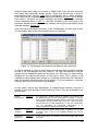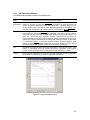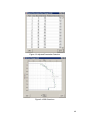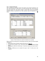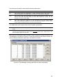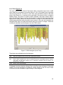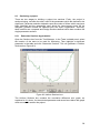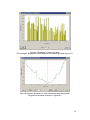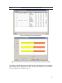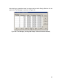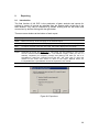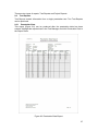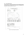
1
User Manual
UK DCP 2.2
Measurement of Road Pavement Strength by
Dynamic Cone Penetrometer
by Simon Done and Piouslin Samuel
Unpublished Project Report
PR INT/278/04
Project Record No R8157
PROJECT REPORT PR/INT/278/04
Measurement of Road Pavement Strength by Dynamic Cone Penetrometer
Simon Done and Piouslin Samuel
Sector:
Transport
Theme:
T2: Reduce overall transport cost by cost effective road rehabilitation
and maintenance
Project Title:
Improved Measurement of Road Pavement Strength by Dynamic
Cone Penetrometer
Project Reference:
R8157
Approvals
Project Manager
Quality Reviewed
Copyright TRL Limited May 2004
This document has been prepared as part of a project funded by the UK Department
for International Development (DFID) for the benefit of developing countries. The views
expressed are not necessarily those of DFID.
The Transport Research Laboratory and TRL are trading names of TRL Limited, a member of the
Transport Research Foundation Group of Companies.
TRL Limited. Registered in England, Number 3142272. Registered Office: Old Wokingham Road,
Crowthorne, Berkshire, RG45 6AU, United Kingdom.
ii
ACKNOWLEDGEMENTS
The development of UK DCP software has been based upon the responses received to
a questionnaire distributed to the members of the International Focus Group (IFG). We
are extremely grateful to those who took the time to complete the questionnaire and
return it to us. We are also grateful to Dr Stephen Morris and James Painter of Tessella
Support Services plc who wrote the software and Yogita Maini of DFID and Phil PageGreen of CSIR, South Africa, who reviewed the project and provided useful feedback.
The TRL team responsible for analysing the questionnaires, designing the software,
writing the user manual and making UK DCP available were Piouslin Samuel, Colin
Jones, Simon Done, Dr John Rolt, Dave Weston and Trevor Bradbury.
May 2004
iii
Contents
1
Introduction .............................................................................................................1
2
Installation ...............................................................................................................5
2.1
Obtaining UK DCP .........................................................................................5
2.2
Installing UK DCP ..........................................................................................5
2.2.1 Installation from CD ...................................................................................5
2.2.2 Installation from Transport Links website ..................................................5
2.3
Uninstalling UK DCP......................................................................................6
3
Start up....................................................................................................................7
3.1
Run UK DCP..................................................................................................7
3.1.1 Start a new project.....................................................................................8
3.1.2 Open an existing project............................................................................9
3.1.3 Closing a project and exiting UK DCP.......................................................9
3.2
Test Manager .................................................................................................9
4
Data input..............................................................................................................11
4.1
Introduction...................................................................................................11
4.2
Site details ....................................................................................................12
4.3
Upper layers.................................................................................................13
4.3.1 Layers removed .......................................................................................13
4.3.2 Upper layer details ...................................................................................14
4.4
Penetration data...........................................................................................16
4.4.1 Site details summary ...............................................................................16
4.4.2 Penetration data.......................................................................................16
4.5
Set-Up ..........................................................................................................20
4.5.1 Analysis ....................................................................................................21
4.5.2 Sectioning.................................................................................................21
4.5.3 CBR Calculation.......................................................................................22
4.5.4 Other Options...........................................................................................23
5 Layer analysis .......................................................................................................24
5.1
Introduction...................................................................................................24
5.2
Analysing Test layers...................................................................................24
5.3
Automatic layer analysis ..............................................................................25
5.4
Manual layer analysis ..................................................................................29
5.5
Analysis of drilled and very strong layers ....................................................36
5.5.1 Drilled layers ............................................................................................37
5.5.2 Very strong layers ....................................................................................39
6 Structural Number calculation ..............................................................................41
6.1
Introduction...................................................................................................41
6.1.1 Upper layers.............................................................................................41
6.1.2 Base and Sub-base Test layers ..............................................................41
6.1.3 Subgrade Test layers...............................................................................42
6.2
Calculating the Structural Number...............................................................42
6.2.1 Upper layers.............................................................................................43
iv
7
6.2.2 Test layers................................................................................................44
6.2.3 SN Calculation Buttons ............................................................................45
6.2.4 Pavement Strength ..................................................................................48
Query ....................................................................................................................50
7.1
Introduction...................................................................................................50
7.2
Making a Query............................................................................................50
7.2.1 Query Parameter .....................................................................................51
7.2.2 Tests Included..........................................................................................51
7.2.3 Query Type...............................................................................................51
7.2.4 Display Options ........................................................................................51
7.3
Displaying the Query results ........................................................................51
7.3.1 Structural Number....................................................................................52
7.3.2 Layer or Pavement Thickness .................................................................53
7.3.3 CBR..........................................................................................................54
8 Sectioning .............................................................................................................56
8.1
Introduction...................................................................................................56
8.2
Sections box.................................................................................................57
8.2.1 Parameters ..............................................................................................57
8.2.2 Tests Included..........................................................................................58
8.2.3 Sections Buttons ......................................................................................58
8.3
Sectioning a project......................................................................................59
8.3.1 Determine Sections by parameter...........................................................59
8.3.2 Determine Design Sections for the project..............................................62
9 Reporting...............................................................................................................66
9.1
Introduction...................................................................................................66
9.2
Test Reports ................................................................................................67
9.2.1 Penetration Data ......................................................................................67
9.2.2 Layer Strength Analysis ...........................................................................69
9.3
Project Reports ............................................................................................71
9.3.1 Section Summary.....................................................................................71
9.3.2 Design Section Properties .......................................................................72
9.3.3 Project Summary .....................................................................................73
10 References ...........................................................................................................74
v
List of Figures
Figure 1.1 DCP instrument ................................................................................................2
Figure 3.1 Flash screen.....................................................................................................7
Figure 3.2 Welcome box....................................................................................................8
Figure 3.3 Test Manager (without test data)......................................................................8
Figure 3.4 Test Manager (with test data and completed analysis)...................................9
Figure 4.1 Test Details box ..............................................................................................11
Figure 4.2 Illustration of Upper layers, Test layers and Removed layers.......................14
Figure 4.3 Penetration Data box (with test data).............................................................16
Figure 4.4 Penetration Data box (with a drilled layer and an extension rod)..................20
Figure 4.5 Set-Up Options box ........................................................................................21
Figure 4.6 Test Manager (showing that test data has been input) .................................23
Figure 5.1 How Automatic analysis works ......................................................................26
Figure 5.2 Layer Boundaries box using Automatic layer analysis ..................................26
Figure 5.3 Test Manager (showing that test data has been analysed)...........................28
Figure 5.4 Layer Boundaries box using Manual layer analysis ......................................30
Figure 5.5 Test Manager (showing that test data has been analysed)...........................32
Figure 5.6 Double intersections .......................................................................................34
Figure 5.7 Negative gradient............................................................................................34
Figure 5.8 Line does not intersect the line of test points.................................................35
Figure 5.9 Line drawn parallel to its intended position ....................................................35
Figure 5.10 Line moved laterally to its intended position ................................................36
Figure 5.11 Lines overlap but do not intersect................................................................36
Figure 5.12 Automatic analysis of a drilled layer.............................................................37
Figure 5.13 Manual analysis of a drilled layer and the use of gaps................................38
Figure 5.14 Automatic analysis of a very strong layer ....................................................39
Figure 5.15 Manual analysis of a very strong layer and the use of gaps .......................40
Figure 6.1 SN Calculation box (before calculating SNs).................................................43
Figure 6.2 Layer Boundaries box.....................................................................................45
Figure 6.3 Adjusted Penetration Data box.......................................................................46
Figure 6.4 CBR Chart box................................................................................................46
Figure 6.5 SN Calculation box (after calculations are complete)....................................48
Figure 6.6 Test Manager (showing that SNs have been calculated)..............................49
Figure 7.1 Query box .......................................................................................................50
Figure 7.2 Structural Number histogram .........................................................................52
Figure 7.3 Layer Thickness histogram ............................................................................53
Figure 7.4 CBR histogram (Minimum).............................................................................54
Figure 7.5 CBR histogram (Less Than) ..........................................................................55
Figure 8.1 Sections box (before sectioning)....................................................................57
Figure 8.2 Uniform Sections box .....................................................................................59
Figure 8.3 Histogram of sectioning data..........................................................................61
Figure 8.4 Uniform Sections box (with one section boundary added) ............................61
Figure 8.5 Sections box (after Sectioning) ......................................................................62
Figure 8.6 Section Summary box ....................................................................................62
Figure 8.7 Design Section Properties box.......................................................................64
Figure 8.8 Section Summary box (with one Design Section boundary added) ..............64
Figure 8.9 Test Manager (showing that Design Sections have been defined)...............65
Figure 9.1 Export box.......................................................................................................66
Figure 9.2 Penetration Data Report.................................................................................67
Figure 9.3 Layer Strength Analysis Report .....................................................................69
Figure 9.4 Section Summary Report ...............................................................................71
Figure 9.5 Design Section Properties Report..................................................................72
Figure 9.6 Project Summary Report................................................................................73
vi
List of Tables
Table 4.1 Penetration rate – CBR relationships ..............................................................22
Table 5.1 Example of penetration data and cumulative difference sum analysis ..........27
Table 6.1 CBR – Strength Coefficient (a) relationships ..................................................42
List of Boxes
Box 1.1 Key points to know before starting to use UK DCP........................................ 4
Box 4.1 Recording the removal of very thick Upper layers........................................ 15
Box 4.2 Calculating adjusted penetration data........................................................... 17
Box 5.1 Should penetration data be analysed automatically or manually? ............... 25
Box 5.2 Corrected analysis of deep surface texture and disturbed soil..................... 29
Box 5.3 Analysis of a drilled layer............................................................................... 38
Box 5.4 Analysis of a very strong but penetrable layer.............................................. 40
Box 6.1 The importance of checking the layer analysis against the CBR Chart....... 47
vii
1
Introduction
When required to assess the strength of a pavement or to design improvement
works, the pavement engineer needs to know as much as possible about the
thicknesses of the existing pavement layers and their condition. In some cases the
quickest and easiest way to do this is to inspect the design to which the pavement
was originally built and perhaps also the as-built records made during construction.
However, designs indicate only an intended construction and as-built records are
often only indicative of the construction work carried out. Furthermore, both designs
and as-built records give no information as to what has happened to the pavement
since construction and the condition it is currently in. To give useful information, it is
therefore necessary to investigate the current pavement condition using some form
of destructive or non destructive testing.
The usual method of destructive testing is to dig test pits at suitable intervals along
the road. These are very useful as pavement thicknesses can be measured and
material removed for testing in a laboratory. However, test pits are expensive to dig
and reinstate and are rarely dug at intervals of less than 2-3 kilometres.
The Dynamic Cone Penetrometer (DCP) (Figure 1.1), is an efficient way of testing
pavement at more frequent intervals. Tests using the DCP generate data which can
be analysed to produce accurate information on in situ pavement layer thicknesses
and strengths. Tests can be carried out very rapidly and test sites can be repaired
extremely easily. A typical DCP test team of 3 people may be able to carry out 20
tests in a day at a spacing of between 50 and 500 metres. The DCP can therefore
give information of sufficient quality and quantity to allow the pavement strength to
be estimated and improvement works designed. Results from DCP tests can also be
used to locate test pits in the most suitable positions.
The DCP consists of a cone fixed to the bottom of a tall vertical rod. A weight is
repeatedly lifted and dropped onto a coupling at the mid-height of the rod to deliver a
standard impact, or ‘blow’, to the cone and drive it into the pavement. A vertical scale
alongside the rod is used to measure the depth of penetration of the cone. The
penetration per blow, the ‘penetration rate’, is recorded as the cone is driven into the
pavement and then used to calculate the strength of the material through which it is
passing. A change in penetration rate indicates a change in strength between
materials, thus allowing layers to be identified and the thickness and strength of each
to be determined. These layers are then grouped together into the pavement layers
of base, sub-base and subgrade, guided by test pit or as-built records if available.
The DCP cannot penetrate some strong surface and base materials such as hot mix
asphalt or cement treated bases. These layers must be removed before the test can
begin and their strength assessed using different criteria.
The strengths of all layers can then be combined into a Structural Number for each
pavement layer and the entire pavement structure. Where tests are repeated along
the pavement, a longitudinal picture of the pavement can be developed which allows
changes in construction and condition to be identified. This data can then be used to
divide the road into homogeneous sections.
1
Figure 1.1 DCP instrument
This manual guides users of this UK DCP software. It has 9 chapters, each
describing one stage or function of its installation and operation.
No.
Title
Description
1
Introduction
2
Installation
Obtain and install UK DCP.
3
Start up
Run UK DCP and open a new or existing project. The term project refers
to a set of related sites, at each of which a penetration test has been
carried out and which will be analysed together. In normal use, a project
will be a single road or a length of apparently uniform construction.
4
Data input
Input site details and penetration data for the tests within a project.
5
Layer
analysis
Analyse the penetration data from a test to identify, and determine the
thicknesses of the distinct Test layers within the pavement. Layer
identification can be carried out manually or automatically.
6
Structural
Number
calculation
Assign the Test layers to specific pavement layers and calculate the
Structural Number of each pavement layer.
7
Query
Produce histograms of strengths and pavement layer thicknesses along
the project. The primary purpose of this function is to identify any errors
made during data entry and analysis.
8
Sectioning
Divide a project into uniform sections.
9
Reporting
Produce reports of the data, analysis and results for printing or export.
2
UK DCP was written in Visual Basic language and uses a Microsoft Access database
to store the data, although it is not necessary for Microsoft Access itself to be
installed on the computer. It will run on Windows 98, NT, 2000 and XP operating
systems and ideally requires a computer with a minimum specification of 400 MHz,
64 MB of memory and 45 MB of free disk space , although it should still run
successfully, albeit slightly more slowly, on a computer of lower specification.
UK DCP is not intended to replace normal engineering judgement. The procedures
used are intended for users who already have a thorough understanding of DCP
analysis and are capable of deciding which method of analysis is most appropriate
for individual situations. The user must be aware of the limitations of this program
and, most importantly, that incorrect data input will lead to incorrect output. The user
should be capable of assessing the accuracy of any results produced. No warranty
can be given on the validity of results and the ultimate responsibility for acceptance
and subsequent use of any results lies solely with the user. TRL Limited cannot
accept any liability for any error or omission.
Some of the limitations of the use of DCP and this package are:
UK DCP can analyse DCP data collected from existing flexible pavements
constructed with unbound materials. Very little difficulty is experienced with the
penetration of granular pavement layers or lightly stabilised material. It is, however,
often not possible to penetrate coarse granular materials, material stabilised with a
high percentage of cement or thick layers of bituminous material. In such cases it is
necessary to drill a hole through the impenetrable layer and then continue gathering
DCP penetration data in the underlying material. Because penetration data can not
be recorded for the drilled layer, it is necessary to estimate and input the strength
coefficient for the layer in order to assess its contribution to the Structural Number of
the pavement.
Thin bituminous layers, such as a surface dressing, can be penetrated by the DCP,
although the data is not used to calculate the strength of such layers, and as such
the strength coefficient must be estimated.
UK DCP cannot analyse penetration data which includes two drilled layers below the
surface. If it proves necessary to drill twice, it is recommended that a test is repeated
or that the test result be analysed manually.
The DCP instrument with an extension rod of 400 mm can be used to a depth of only
1200 mm. Although the instrument can be extended beyond this depth, with
additional extension rods or extension road longer than 400 mm, it is not
recommended that this is done as friction between the rod and the soil can give
unreliable data. However, UK DCP has been designed to accept data up to a
maximum depth of 1500 mm.
The output from DCP results is controlled by the user as follows:
• Selecting an appropriate CBR – DCP penetration relationship as explained in
4.5.3. CBR Calculation.
• The user’s identification of the base, sub-base and subgrade layers as
explained in 5. Layer Analysis.
• Selection of appropriate parameters for dividing the project into shorter
sections of uniform strength as explained in 8. Sectioning.
3
UK DCP is available free of charge to all who wish to use it.
Box 1.1 Key points to know before starting to use UK DCP
Context sensitive help is available at all stages. This manual can also be displayed and
printed through the Help menu at the top of the main window.
Data and results do not have to be saved manually. Whenever data is entered into a box and
the box is closed by clicking an OK button, its contents are automatically saved.
Only one set of penetration tests (a ‘project’) can be opened at any one time, but many of
those tests can be examined simultaneously and compared.
When a number of windows and boxes are open, they can be selected for display using the
Window menu at the top of the main window.
In this manual all software images have been taken from a single project. Two images at the
same chainage represent the same data and later sectioning images are based upon
penetration data in earlier images.
4
2
Installation
2.1
Obtaining UK DCP
UK DCP can be obtained by contacting TRL:
TRL Limited
Crowthorne House
Nine Mile Ride
Wokingham
Berkshire
RG40 3GA
United Kingdom
Tel: + 44 (0) 1344 770187
Fax: +44 (0) 1344 770356
Email: [email protected]
Web: www.trl.co.uk
Alternatively, UK DCP is available on the Road Engineering for Development CD,
distributed by TRL, or as a download from the Transport Links website. The address
of this website is www.transport-links.org/ukdcp
2.2
Installing UK DCP
Before installing UK DCP, it is recommended that any earlier versions of the software
are uninstalled (2.3) and, if there are any data files from previous analysis to be
saved, the UK DCP directory is moved from the Program Files directory to a different
location. The total size of the files which must be downloaded for installation is
11.6MB.
2.2.1
Installation from CD
This procedure will install UK DCP, all necessary third party software and help files
onto the user’s computer. For computers with Windows 2000 or NT, follow steps 1 to
4 below. For computers with Windows 98 or XP, follow steps 1 to 6.
1. Open the UK DCP folder on the CD.
2. Double-click or run the file named ‘setup.exe’.
3. When prompted, select the directory in which UK DCP will be installed. By
default, ‘C:\Program Files\UKDCP’ is selected.
4. When the setup program is complete, a new item, ‘UK DCP’, will be added to
the Start/Programs menu.
5. In the UK DCP folder, double-click or run the file named ‘MDAC_TYP.exe’.
6. When this setup program is complete, reboot the computer.
2.2.2
Installation from Transport Links website
The procedure to download all relevant files and install UK DCP, all necessary third
party software and help files onto the user’s computer from the Transport Links
website is very simple. Click on UK DCP Installer. Downloading and installation will
take place automatically. For computers with Windows 98 or XP, it is then necessary
to click on ‘MDAC_TYP.exe’, wait for the setup programme to finish and reboot the
computer.
5
2.3
Uninstalling UK DCP
This procedure will uninstall UK DCP from the user’s computer. It may vary slightly
depending upon which Windows operating system is installed on the computer.
1.
2.
3.
4.
5.
6.
Select Settings from the Start menu.
Select Control Panel.
Double-click Add or Remove Programs.
Highlight the version of UK DCP to be removed.
Click Change/Remove.
This will not completely delete all files. When uninstallation is complete, open
Windows Explorer and then navigate to the folder in which UK DCP was
installed. Delete the folder and its contents. If the warning “Renaming, moving
or deleting ‘ukdcp’ could make some programs not work. Are you sure that
you want to do this?” is generated, click Yes and continue with the deletion.
6
3
Start up
This chapter describes how to run UK DCP and introduces the Test Manager.
3.1
Run UK DCP
UK DCP can be run by either clicking a desktop icon or through the Programs menu
on the Start button. After a brief Flash screen (Figure 3.1), the Main window will open
with a Welcome box (Figure 3.2). The Welcome box allows a new or existing project
to be opened and also contains a list of the most recently used projects. The same
options are available in the File menu at the top of the main window.
Figure 3.1 Flash screen
7
Figure 3.2 Welcome box
3.1.1
Start a new project
Click New Project in the Welcome box or in the File menu at the top of the main
window. This will generate a Save New Project As box. Give a name to the new
project, select a folder in which to save it and click Save. The project will be
automatically given a .ukdcp file extension and saved in the selected folder. An
empty Test Manager box (Figure 3.3) will open for the new project with its name at
the top. Since only one project can be open within UK DCP at any time, if a project is
currently open and a new project is named and saved, a message will be generated
seeking confirmation that the current project should be closed. If Yes is clicked, the
current project will be closed and the new project opened.
Figure 3.3 Test Manager (without test data)
8
3.1.2
Open an existing project
Click Open Existing Project in the Welcome box or Open Project in the File menu at
the top of the main window. This will generate an Open Existing Project box in which
the file of the required project can be found and selected. Highlight the file and click
Open. A Test Manager filled with the existing data and analysis will open (Figure 3.4
shows a Test Manager of a project which has been fully analysed). Alternatively,
double-click on the required file in the Recent Files list in the Welcome box or in the
File menu and the Test Manager will open. Since only one project can be open within
UK DCP at any time, if a project is currently open and an existing project is selected,
a message will be generated seeking confirmation that the current project should be
closed. If Yes is clicked, the current project will be closed and the selected project
opened.
Figure 3.4 Test Manager (with test data and completed analysis)
3.1.3
Closing a project and exiting UK DCP.
Only one project can be run by UK DCP at any time. To close a project, click Close
in the Test Manager. A box will be generated seeking confirmation. Click Yes to
close the project. To exit UK DCP, click Exit in the File menu at the top of the main
window. A box will be generated seeking confirmation. Click Yes to exit.
3.2
Test Manager
The Test Manager (empty: Figure 3.3, or complete: Figure 3.4) is used to store all
data from the project and manage data entry, layer analysis, strength calculations,
queries and project sectioning. Each row of the table in the Test Manager represents
one penetration test and shows the progress that has been made in analysing the
data from both the individual test and the entire project.
9
The table in the Test Manager has five columns.
Test number
Tests are automatically numbered in chainage order from 1 upwards. If more
than one test is carried out at the same chainage, they are ordered according
to their location (carriageway; shoulder; verge; lay-by / other – see 4.2 below).
If more than one test is carried out at the same chainage in the carriageway,
they are ordered according to their lane number and offset (see 4.2 below). If
more than one test is carried out at the same chainage off the carriageway,
they are ordered according to their offset. There is no limit to the number of
tests that can be entered in a single project. If a test is added out of sequence
or if a test is deleted, the numbering is automatically corrected.
Chainage
(km)
The chainage at which the test was carried out, measured in kilometres.
Analysis
The date when the test data was analysed to identify layers. The cell is blank
if the data has not yet been analysed.
SN
calculation
The date when the Structural Numbers of the pavement layers were
calculated. The cell is blank if these have not yet been calculated.
Sectioning
The date when Design Sections were determined for the project. The cell is
blank if the project has not yet been sectioned.
There are eleven buttons below and to the right of the table. Warning messages are
generated in response to Delete, Reset and Close. In each case, click Yes to
continue with the operation.
Set-Up
Record, review or edit information about how each test is carried out, analysed
and displayed. This button is inactive if tests are being reviewed, edited or
analysed.
Add
Input data from a new test into the Test Manager.
Delete
Delete a selected existing test from the Test Manager. This button is inactive if
tests are being reviewed, edited or analysed.
Reset
Remove the layer analysis, SN calculation and sectioning from all tests in the
project.
Close
Close a project. UK DCP remains open so that another project can be analysed.
Help
Open this manual on the screen at the appropriate section.
Data
Review or edit the details and data of a selected test.
Analyse
Identify layers from the test data.
Calculate
SN
Calculate the Structural Numbers of the pavement layers. This button is inactive
if layers have not yet been identified from the test data.
Query
Graphically present the strengths and layer thicknesses along the length of an
entire project. This button is inactive if the Structural Numbers have not yet
been calculated for all the tests in the project.
Section
Divide a project into sections according to a selection of parameters. This button
is inactive if the Structural Numbers have not yet been calculated for all the
tests in the project.
10
4
4.1
Data input
Introduction
This chapter describes how to input data for the penetration tests within a project.
For each penetration test, the following are required.
• Site details – information about the site where the test was carried out.
• Upper layers – information about the upper layers which cannot be analysed
by a DCP.
• Penetration data – data which records the number of blows of the DCP and
the depth of penetration
• Set-Up – information about how each test is carried out, analysed and
displayed.
To input data from a new test, click Add in the Test Manager. To review or edit data
from a test which has already been inputted, highlight the test in the Test Manager
and click Data. Both actions will bring up the Test Details box (Figure 4.1) for that
test. At any point during data input, Cancel can be clicked to cancel the entered
information. This will generate a box asking if the changes that have been made
should be saved. Clicking No will cancel any changes that were made.
Figure 4.1 Test Details box
11
4.2
Site details
The top panel of the Test Details box is titled Site details and records information
about the site where the test was carried out. The panel has a number of fields.
These are mandatory (M), optional (O) or filled in automatically (A).
Test
number
A
This field is filled in automatically according to the chainage and
location of the test, as described in 3.2 above.
Chainage
(km)
M
It is important that all tests within a project use the same chainage
datum.
Location
M
Although penetration tests are normally carried out in the
carriageway of a road, it may be necessary to measure the strength
of the construction off the carriageway line. When results are
analysed, it will be necessary to distinguish between these locations
so that, for example, carriageway improvement works are not
designed using layer strengths measured in a soft verge. Therefore,
using the pull-down menu, select the location of the test from
carriageway, shoulder, verge and lay-by / other. Carriageway is the
default location.
Lane
number
O
It may be necessary to record in which lane of a road a test was
made. Thus this field may be required if tests are being carried out
on a road with more than one lane in each direction. Any normal local
convention can be used for numbering lanes.
Offset
(m)
O
This refers to the offset from a datum line along the road. It is normal
to use the carriageway edge as the datum, although the centre line of
the road could be used instead.
Direction
O
This is the traffic direction of the lane where the tests are being
carried out. Direction does not need to be recorded on a single lane
road. The field is limited to 25 characters.
Zero
error
(mm)
M
The zero error is the reading on the vertical scale of the DCP when
the cone is sitting on a flat surface and is a result of the way in which
the instrument is manufactured and assembled. The zero error is
measured by placing the DCP on a smooth, level, hard surface,
lowering the cone to the surface and reading the scale. This should
be done whenever the DCP is prepared for use and, ideally, before
every new series of tests. The zero error should be entered for every
test.
Test date
M
This defaults to today’s date, but can be changed using the pull down
calendar.
Remarks
O
These can be either typed or copied and pasted as required. The
field is limited to 60 characters.
If the details of a test have already been entered, click Edit to be able to make
changes, although if the data has already been analysed, a box will be generated
warning that editing the data will delete this analysis.
12
4.3
Upper layers
UK DCP uses penetration data to calculate the strength of most pavement layers.
However, some layers are too thin, strong or impenetrable for relationships between
penetration rate and strength to be derived. In this case, the strength of the layer is
assessed from the type of the layer and its condition. This applies to layer types such
as:
Surface
• Thin bituminous seal
• Hot mix asphalt
• Concrete
• Other surface
Base
• Cement treated base
• Bituminous base
• Coarse granular base (such as Water Bound Macadam)
Since these layers are always found at the top of a pavement, they are referred to as
Upper Layers. Layers whose strength can be calculated from penetration data are
referred to as Test Layers.
The calculation of layer and pavement strength for Upper layers and Test layers is
explained in detail in 6.1 below.
The bottom panel of the Test Details box (Figure 4.1) is titled Upper layers. A
selection must be made and a table must be completed.
4.3.1
Layers removed
Although Upper layers such as a thin bituminous seal can be penetrated by a DCP,
some layers, such as hot mix asphalt or a cement treated base cannot be
penetrated. It is necessary to remove these layers by drilling or cutting out before the
test can be carried out. When inputting data, the number of upper layers which were
removed should be entered. UK DCP can accept the removal of 0, 1 or 2 layers. If
more than two have been removed, it is necessary to group them into two or fewer
removed layers. Figure 4.2 illustrates the differences between Upper layers, Test
layers and removed layers for a variety of pavement constructions.
13
No layers removed
Upper
Layers
Unpaved
Thin
Bituminous
Seal
One layer
removed
Two layers
removed
HMA
HMA
Concrete
Base
Test
Layers
a)
b)
c)
d)
e)
Pavement a) is unpaved. All layers can be analysed using penetration data. In this respect
there are no Upper layers, although in subsequent stages, such as the SN
Calculation box, described in 6.2 below, and the Penetration Data Report, described
in 9.2.1 below, Unpaved will be recorded as an Upper layer so that the user is
reminded of the surface type.
Pavement b) has a thin bituminous seal over a granular base. The thin seal cannot be
analysed using penetration data and is therefore an Upper layer. Since the material
can be penetrated by a DCP cone, it is not necessary to remove the layer. Therefore
for this test there is one Upper layer but it is not removed.
Pavement c) has an HMA surface over a granular base. The HMA cannot be analysed using
penetration data and is therefore an Upper layer. The material cannot be penetrated
by a DCP cone and so must be removed. Therefore for this test, there is one Upper
layer and it is removed.
Pavement d) has a concrete surface over a granular base. As for pavement c), the concrete
is an impenetrable Upper layer and must be removed. However, rigid pavements are
not analysed using Structural Numbers and therefore, although UK DCP calculates
the Structural Numbers, only the strengths of the individual Test layers can be used.
Pavement e) has an HMA surface over a base such as water bound macadam. Both layers
are impenetrable. Therefore for this test, there are two Upper layers and both are
removed.
Figure 4.2 Illustration of Upper layers, Test layers and Removed layers
4.3.2
Upper layer details
For each Upper layer, the following information must be entered into the table.
Layer
This will be prompted according to the number of layers which have been
removed. If 0 or 1 Upper layers have been removed, only one layer will be
prompted and will be defined as Surface. If two Upper layers have been
removed, two layers will be prompted. The first will be defined as Surface and
the second as Base.
Type
Options will be offered from the list in 4.3 according to whether the layer is a
surface or a base and whether or not the layer has been removed. If no Upper
layers have been removed, Unpaved will also be offered as an option. Gravel
and earth surfaces can be analysed using penetration data and so are not
technically Upper layers, but will be recorded as such so that the surface type
will be listed when reports are generated. If the layer is Unpaved, the final three
columns are automatically left grey and inactive since the layer will be analysed
using penetration data rather than condition. If the layer is concrete, the final two
14
columns are automatically left grey and inactive since rigid pavements are not
analysed using Structural Numbers.
Thickness
(mm)
Thicker layers contribute more strength to the pavement. UK DCP will generate
a prompt if the value is too high or low for that type of layer. If the layer is a thin
bituminous seal, a default thickness of 20 mm will be automatically entered. Box
4.1 provides guidance on how to record the removal of very thick Upper layers.
Condition
The observed condition of a surface layer is used to determine its strength
coefficient. If the condition is known, use the pull down menu to select a
condition. Then click in the strength coefficient box and the value will be entered
automatically. If condition is unknown, or it is already known which strength
coefficient to use, enter a condition of ‘Unknown’ and then manually enter the
value. If there are two Upper layers, it is often difficult to assess the condition of
the base. Therefore a condition of Unknown is automatically generated for the
base and the strength coefficient must be entered manually.
Strength
coefficient
The strength coefficient is required to calculate the contribution of the layer to the
strength or Structural Number of the pavement. It can be entered manually or
generated automatically from the condition of the layer. If it is entered manually,
UK DCP checks that it is within a realistic range for the layer type selected.
Box 4.1 Recording the removal of very thick Upper layers
UK DCP can be used to analyse granular layers underneath thin or thick bituminous
surfacing. The maximum allowable thickness of HMA or bituminous layer is 350 mm since
this is a normal upper limit for this material type. However, if a greater thickness of asphalt is
removed before the DCP can be used, it is recommended that it is recorded in two layers; a
surface layer of HMA with its observed condition and automatically generated strength
coefficient followed by a base layer of bituminous material with unknown condition and a
strength coefficient manually entered to be equal to that of the surface layer. The maximum
total thickness of the removed asphalt is therefore 700 mm which should be sufficient for all
roads.
There are five buttons below the Upper Layer panel.
Help
Open this manual on the screen at the appropriate section.
Penetration
Data
Open a Penetration Data box so that test data can be entered.
Clicking this button also checks that all data entered into the
Test Details box is valid. Any invalid entries must be corrected
before the Penetration Data box can be opened.
Cancel
Close the box and return to the Test Manager without saving
the changes that have been made since the box was created or
opened for editing. A box is generated seeking confirmation
that the changes should be saved.
Edit
Close
Visible if
data has
already been
entered and
saved
Edit the data in the box. If the current data has already been
used to identify layers, a box will be generated warning that
editing the data will delete this analysis.
Return to the Test Manager without making any edits.
15
4.4
Penetration data
After completing the Test Details box with Site details and Upper layer information,
click Penetration Data to open an empty Penetration Data box. This box has two
panels.
Figure 4.3 Penetration Data box (with test data)
4.4.1
Site details summary
This panel provides a summary of the site details which have already been entered.
These details cannot be edited.
4.4.2
Penetration data
During a DCP test, the cone is driven into the pavement under repeated blows. The
record from a test consists of a number of test points. At each test point the number
of blows since the last test point is recorded and the total penetration of the cone is
measured.
It is recommended that the penetration of the cone should be measured at
increments of about 10 mm. However, it is usually easier to measure penetration
after a set number of blows. It is therefore necessary to change the number of blows
between measurements according to the strength of the layer being penetrated. For
good quality granular bases, measurements every 5 or 10 blows are normally
sufficient, but for weaker sub-bases and subgrades, measurements every 1 or 2
blows may be required. There is no disadvantage in taking too many readings but if
too few are taken, there is a danger that weak spots will be missed and layer
boundaries will be difficult to identify.
16
This data is entered into the table in this panel. Each row in the table represents one
test point. The table has four columns.
Point
number
The number of each test point. If a point is inserted or deleted, the numbering is
automatically corrected. A maximum of 250 test points can be entered for each
DCP test. If more than 250 have been recorded, it is likely that the cone hit an
impenetrable object such as a stone, in which case the data is of no use.
Blows
The number of blows given to the cone to drive it from the previous point to the
current point. The number of blows at the first test point is automatically set at
zero. A maximum of 25 blows are permitted between each test point. If more
blows are given, changes in depth are likely to be too high for useful results to
be calculated.
Penetration
depth (mm)
The depth at the current point, as read off the DCP scale. The depth of the first
test point, the ‘initial reading’, is recorded before any blows have been given.
Since the zero error (see above) is measured when the DCP is placed on a
smooth and level surface, it is impossible for the initial reading to be less than
the zero error. The initial reading also includes the thickness of all removed
layers. It will not be accepted if it is less than the sum of the zero error and the
thicknesses of the removed layers as if so, it is likely to be an error. Note that in
Figure 4.3 the initial reading (78) is greater than the sum of the zero error (33)
and the thickness of the removed layer (40). A maximum penetration depth of
1500 mm is allowed. If the cone has penetrated further than this, it is likely that
friction along the rod is significantly reducing the penetration rate of the cone, in
which case the data is unreliable and should not be used.
Comments
Comments are entered automatically if an impenetrable layer was drilled or if
an extension rod was used (see below).
Box 4.2 Calculating adjusted penetration data
In order to analyse a penetration test, two corrections to the recorded depths are necessary.
• The zero error is subtracted from all depths.
• The length of an extension rod (see below), where used, is added to the depths of all test
points recorded after the rod was fitted.
UK DCP makes these corrections automatically. The corrected data is referred to as
‘adjusted data’.
To the right of the table are three buttons. These are used when entering or deleting
penetration data.
Insert
Insert a test point into the data. Highlight the row below which the new test is
required and click Insert. Then enter the data from the new test point into the empty
row.
Delete
Delete a test point. Highlight the test point to be deleted and click Delete. The first
test point cannot be deleted.
Paste
This button is used to transfer the penetration data of one test from a spreadsheet
into the panel, for example if the data was entered on site into a palm top or other
device. The data should be entered into the spreadsheet in two columns:
incremental blows and total depth (mm). Highlight and copy the two columns. Then
return to UK DCP and click Paste. It is not necessary to position the cursor in the
first row before clicking Paste.
17
Penetration data can also be entered manually. On the first row type the penetration
depth before any blows have been given and then use Tab or Enter on the keyboard
to enter data in one cell after another.
There are six buttons below the table.
Help
Open this manual on the screen at the appropriate section.
Test
Details
Return to the Test Details box.
OK
Save the data entered into the Test Details and Penetration Data
boxes and return to the Test Manager. If the test was a new test,
a further Test Details box will be generated. If the test had been
entered earlier and the data was being reviewed or edited, a
further box is not generated.
Cancel
Close the box and return to the Test Manager without saving the
changes that have been made since the box was created or
opened for editing. A box is generated seeking confirmation that
the changes should be saved.
Edit
Close
Visible if
data has
already
been
entered
and saved
Edit the penetration data. If the current data has already been
used to identify layers, a warning will be generated that editing
the data will delete this analysis.
Return to the Test Manager without making any edits.
18
A comment will be entered automatically if a layer was drilled or an extension rod
was used.
Drilled layer
If an impenetrable layer has been drilled, the penetration data will include one point
recorded before the DCP was removed and another point recorded after the layer
was drilled. There will be a difference in depth between these points, although no
blows will have been recorded. If this data is pasted from a spreadsheet, a comment
will automatically appear in the Comment column stating ‘Layer Drilled’ (see Figure
4.4). If data is edited or a point is inserted or deleted to give a depth difference with
no recorded blows, a prompt will ask if a layer has been drilled. If Yes is clicked, the
same comment is entered; if No is clicked, the Blows entry is deleted and should be
re-entered. Drilled layers are recorded and presented in later stages of the analysis.
Only one drilled layer can be recorded in a test. If two layers were drilled to achieve
the desired penetration depth, it is likely that the material was excessively disturbed,
in which case the data is unreliable and should not be used.
Extension rod
In normal operation, a DCP can penetrate to 800 mm. It is possible to add an
extension rod to allow the DCP to penetrate further. In this case, one point will be
recorded before the DCP was removed and another after the extended DCP was
reinserted. The second point will have a numerically lower reading than the first, and
no blows will have been recorded. If this data is pasted from a spreadsheet, a
comment will automatically appear stating ‘Extension Rod Added’ (see Figure 4.4). If
data is edited or a point is inserted or deleted to give a point with no blows and an
apparent reduction in depth, a prompt will ask if an extension rod has been added. If
Yes is clicked, the same comment will appear; if No is clicked, the Blows entry is
deleted and should be re-entered. UK DCP will take account of the use of an
extension rod, determine the length of the rod from the difference between the two
depth readings and adjust the penetration data accordingly. If there is an apparent
reduction in depth before 400 mm of penetration has been reached, the prompt will
not be generated since it is unlikely that an extension rod was added when depths
were small. A reduction in depth before 500 mm is probably due to an error in the
data and an error message will be generated. Only one layer can be recorded as
being due to the use of an extension rod since if further extension rods are used, it is
likely that friction along the rod is significantly reducing the penetration rate of the
cone, in which case the data is unreliable and should not be used.
19
Figure 4.4 Penetration Data box (with a drilled layer and an extension rod)
4.5
Set-Up
Set-Up is used to record information about how each test is carried out, analysed
and displayed.
It is recommended that the set-up function is used as follows. After data from the first
test of a project has been added to the Test Manager, highlight the test and click SetUp in the Test Manager or in the Modules menu at the top of the main window. This
will display the Set-Up Options box (Figure 4.5) for the first test. The box will contain
a number of default settings. Make any changes as required and click Update Set-Up
to save these changes and return to the Test Manager. This will assign that set-up
information to the first test. As further tests are added, they will be automatically
assigned the same set-up information. If at any stage the Set-Up information is
changed and updated, this new set-up information will be assigned to all subsequent
tests. To revert to the default set-up information, click Default and then Update SetUp.
20
Figure 4.5 Set-Up Options box
If a number of tests have been added to the Test Manager, or even if analysis of the
data has already begun, it is possible to return to the Test Manager and change the
Set-Up information for a single test. This may be done if a chosen method of analysis
or display is unsuitable for the data. Highlight the test, click Set-Up, make the
required changes and click Update Set-Up. If analysis of that test has already been
carried out, a box is generated warning that the analysis will be deleted. It should be
noted that if more tests are added, they will retain this updated Set-Up information.
There are four buttons in the Set-Up Options box.
Help
Open this manual on the screen at the appropriate section.
Default
Revert to the default set-up information, as defined below.
Update Set-Up
Save amended set-up information, as described above.
Cancel
Close Set-Up and return to the Test Manager without saving any changes.
The Set-Up Options box has four panels.
4.5.1
Analysis
Layers can be identified either automatically by UK DCP or manually by the user.
This panel allows the method of identification to be selected. The default is automatic
(‘system’) analysis.
4.5.2
Sectioning
A project can be divided into sections either automatically by UK DCP or manually by
the user. This panel allows the method of identification to be selected. Automatic
sectioning is currently disabled. The default is manual (‘user’) sectioning.
21
4.5.3
CBR Calculation
The strengths of Test layers are calculated by converting the penetration rate (mm
per blow) to a California Bearing Ratio (CBR) value and then from the CBR value to
a strength coefficient and finally to a Structural Number. A number of relationships
between penetration rate and CBR value have been derived and are given in Table
4.1. Some of these are used when the DCP cone has an angle of 60°, others when
the cone has an angle of 30°. The relationship and the cone angle are selected on
this panel. The user’s organisation should provide guidance as to which relationship
should be used or whether a new relationship for the local conditions should be
developed. The default is the TRL relationship for a 60° cone.
The conversion of CBR value to strength coefficient and Structural Number is
described in Chapter 6.
Table 4.1 Penetration rate – CBR relationships
Cone
angle
Name of relationship
60°
cone
TRL
(1)
Relationship
Log10(CBR) = 2.48 – 1.057 Log10(pen rate)
(2)
CBR = 410 (pen rate)
Kleyn (pen rate = 2
mm/blow)
(3)
CBR = 66.66 (pen rate) – 330 (pen rate) + 563.33
Expansive Clay
(4)
Method
Log10(CBR) = 2.315 – 0.858 Log10(pen rate)
Kleyn (pen rate > 2
mm/blow)
100% Planings
(5)
-1.27
2
Log10(CBR) = 1.83 – 0.95 Log10(pen rate)
50% Planings
Log10(CBR) = 2.51 – 1.38 Log10(pen rate)
User-Defined
Log10(CBR) = [constant] – [coefficient] Log10(pen rate)
Constant and Coefficient can be defined by the user
30°
cone
Smith and Pratt
User-Defined
(6)
Log10(CBR) = 2.555 – 1.145 Log10(pen rate)
Log10(CBR) = [constant] – [coefficient] Log10(pen rate)
Constant and Coefficient can be defined by the user
(pen rate is the penetration rate measured in millimetres per blow)
22
4.5.4
Other Options
When penetration data is being analysed, a graph of penetration depth against the
number of blows given to the DCP is used to identify layers of different materials and
the boundaries between them. The items in this panel allow two changes to be made
to this graph which may help in identifying layers.
As-Built Thickness
It is sometimes difficult to identify layers from a penetration graph and, even if layers
can be seen, it can be difficult to be sure whether the layer is part of the base, subbase or subgrade. If actual information on materials and layer thicknesses is
available, layer identification from penetration data can be much easier. This
information can come from records made when the pavement was being constructed
or from test pits dug alongside and within the project. Neither source of information
will accurately predict the layers at each test site, but they can provide useful
guidance. If as-built or test pit information is available, click in the As-Built Thickness
Known? box and enter the recorded thicknesses for the Surface, Base and Subbase. These will be displayed on the penetration graphs, as shown in, for example,
Figure 5.2 and Figure 5.4. The default is to not display as-built thicknesses.
Colours
Different colours are used to indicate different elements of the penetration graph.
They can be changed if required, for example if a printer does not print a particular
colour well. The defaults are Data Point – dark green; Test Layers – dark blue;
underside of Upper Layers – bright blue; Drilled Layer – red.
After data from penetration tests has been input, the Test Manager is as shown in
Figure 4.6.
Figure 4.6 Test Manager (showing that test data has been input)
23
5
5.1
Layer analysis
Introduction
A typical graph of penetration depth against the cumulative number of blows given to
the DCP shows a line of varying gradient. The gradient is equal to the penetration
rate of the cone as it is driven into the pavement.
For Test layers, it is possible to derive relationships (4.5.3) between the penetration
rate and the strength of the material through which the cone is passing. The gradient
of the line can therefore be used to calculate the material strength. Changes in the
gradient of the line indicate boundaries between materials of different strengths and
hence the thicknesses of layers of different strengths.
Upper layers are often too thin, strong or impenetrable for their strength to be
determined from the penetration rate. Instead, the strength of an Upper layer is
estimated from the type of the layer and its condition, and its thickness is taken from
as-built records, test pit data or by measuring the thickness of a layer removed
during the DCP test.
This chapter describes how the thicknesses of Test layers are determined from
penetration graphs; Chapter 6 then describes how the strengths of Upper layers and
Test layers are calculated.
The penetration graph can be analysed automatically or manually according to the
selection made when defining Set-Up information (4.5.1).
5.2
Analysing Test layers
Begin layer analysis from the Test Manager. Highlight a test which has not yet been
analysed and click Analyse in the Test Manager or in the Modules menu at the top of
the main window.
This will open a Layer Boundaries box. It contains a graph of adjusted penetration
depth (data adjustment is explained in Box 4.2) against the cumulative number of
blows given to the DCP. All test points are plotted onto the graph. The gradient of the
line of test points is the penetration rate of the cone and hence the strength of the
material at that depth. A shallow gradient indicates strong material, a steep gradient
indicates weak material and changes in gradient indicate a layer boundary between
Test layers of different strengths.
The other information displayed on the graph depends upon whether layer analysis
will be carried out automatically or manually. These two alternatives are compared in
Box 5.1 and described in detail below.
24
Box 5.1 Should penetration data be analysed automatically or manually?
UK DCP allows penetration plots to be analysed automatically or manually. Each method has
advantages and disadvantages.
Automatic analysis
Advantages
Quicker than manual analysis.
Disadvantages
The user has no control over where layer boundaries are located.
Assigns a strength coefficient to a drilled layer.
Summary
Automatically identified layer boundaries of a complex plot may be located inappropriately.
Automatic analysis is therefore recommended when the penetration plot has a simple shape.
Manual analysis
Advantages
User has more control over where layer boundaries are located.
The use of gaps can improve the analysis of drilled and strong layers.
Disadvantages
Slower than automatic analysis.
Summary
Manual analysis is recommended when the penetration plot has a complex shape, the
analysis of which the user would like to have some control over. It is also recommended if an
atypical item such as a large stone slowed down the penetration or had to be drilled.
5.3
Automatic layer analysis
The automatic layer analysis procedure first calculates the penetration rate at each
test point and the average penetration rate for the entire test. For each test point it
then calculates the value of the average rate minus the rate at that point. These
values are then summed in turn starting at the first test to find the cumulative
difference sum at each point. By the nature of the calculation, this sum will be zero at
the final test point. At one point this sum will reach a maximum absolute value. The
depth of the point at which the sum reaches this maximum value is defined as the
first Test layer boundary. This procedure has a similar effect to drawing a straight
line from the first point to the last point and finding the depth of the intermediate point
which is furthest from this straight line (as shown in Figure 5.1).
25
Figure 5.1 How Automatic analysis works
The procedure is then repeated for the test points above this first boundary and for
the points below it. In this way the second and third boundaries can be identified.
The procedure is repeated until the points between any two boundaries do not
exhibit sufficient fluctuation from a straight line to allow a further boundary to be
identified with any degree of confidence. An automatically analysed penetration plot
is shown in Figure 5.2.
Figure 5.2 Layer Boundaries box using Automatic layer analysis
26
To illustrate automatic layer analysis, Table 5.1 contains penetration data to a depth
of 225 mm. The data is analysed in the table to show how a change from strong to
weaker material can be identified at a depth of 75 mm. Figure 5.1 contains a graph of
the data in this table. It shows how the point with the greatest cumulative difference
sum is also the point which lies furthest from a straight line from the first point to the
last point. The first Test layer boundary has been automatically generated and is
shown on the graph.
Table 5.1 Example of penetration data and cumulative difference sum analysis
Point
Blows
1
2
3
4
5
6
7
8
9
10
11
0
5
5
5
5
5
5
5
5
5
5
Adjusted pen
depth
0
14
29
46
62
75
107
133
164
196
225
Pen rate
(mm/blow)
2.8
3.0
3.4
3.2
2.6
6.4
5.2
6.2
6.4
5.8
Av. Pen
rate
4.5
4.5
4.5
4.5
4.5
4.5
4.5
4.5
4.5
4.5
Av. Pen rate –
pen rate
1.7
1.5
1.1
1.3
1.9
-1.9
-0.7
-1.7
-1.9
-1.3
Cumulative
difference sum
1.7
3.2
4.3
5.6
7.5 ? maximum value
5.6
4.9
3.2
1.3
0
Five points should be noted when using automatic layer analysis.
• Boundaries can be identified only at depths corresponding to actual test
points.
• The strength of a layer is calculated by the gradient of a straight line from the
intersection of its upper boundary with the line of test points to the
intersection of its lower boundary with the line of test points.
• There are three situations where minor corrections are made to the analysis
in order to prevent inaccurate calculation of the thickness of the first Test
layer. These are described in Box 5.2.
• Box 5.3 below recommends when automatic layer analysis should be used
for penetration data containing drilled layers.
• Box 5.4 below recommends when automatic layer analysis should be used
for penetration data containing strong but penetrable layers.
The following items are displayed in the Layer Boundaries box if automatic layer
analysis has been selected. The colours of some of the items depend upon selection
made when defining Set-Up information.
Maximum
layers
message
When the box is opened, a message will be generated giving the maximum
number of Test layers which can be identified from the data using the above
procedure. Click OK to delete this message. If 10 Test layers can be identified
(the limit set by UK DCP), a message is not generated.
First layer
boundary
The first layer boundary identified using the above procedure is shown with a
horizontal line.
Number of
Layers field
The number in this box is the number of Test layers currently being shown.
Clicking the Up and Down arrows increases and decreases this number and
adds or removes layer boundaries from the graph. The number can be
increased up to the number which was shown in the Maximum layers
27
message. Unless a drilled layer is present, this number is initially 2.
Upper layer
line
A dashed line indicates the underside of the Upper Layers.
Drilled
layers
If a layer has been drilled, it will be marked on the graph with two horizontal
dotted lines, but the first automatic layer will not be shown. The Number of
Layers field will therefore initially show 3, the portion above the drilled layer,
the drilled layer itself and the portion below. An automatically analysed drilled
layer is shown in Figure 5.12 below.
As-built
layers
If as-built or test pit information was entered into the Set-Up of the test (4.5.4),
these layers are shown, separated by dotted lines.
Show
Gridlines
A check box is provided to allow gridlines to be displayed or removed.
Adjusted
Data button
Click this button to generate a box showing the penetration data (Figure 6.3).
This data has been adjusted as described in Box 4.2. The box also includes
the average penetration rate between successive points. This box is
generated to guide the identification of Test layers and cannot be edited.
Help button
This button opens this manual on the screen at the appropriate section.
OK button
This is used to accept and save the layer boundaries and return to the Test
Manager.
Cancel
button
This is used to cancel the analysis. If changes have been made to the
analysis, a box is generated which offers an opportunity to save the changes.
Layer
descriptions
When the cursor is placed over the graph, a small box is generated. This box
gives the number of the Test layer, its thickness (mm) and the average
penetration rate for the layer.
Point
descriptions
When the cursor is placed over a test point, a small box is generated. This
box gives the cumulative blows and the adjusted depth of the point.
Add or remove layer boundaries from the graph until satisfied that the data has been
adequately analysed. In Figure 5.2 five Test layers appear sufficient. Adding further
layers does not increase the precision of the analysis. Note that identified Test layers
matching previously defined as-built layers is a useful check on the analysis.
Click OK to save the analysis and return to the Test Manager. It will be seen (Figure
5.3) that today’s date will be in the Analysis column for that test.
Figure 5.3 Test Manager (showing that test data has been analysed)
28
It is possible to examine the graph and possibly edit the analysis of a test for which
layers have already been identified. Highlight the test in the Test Manager and click
Analyse. The Layer Boundaries box will be opened and the penetration graph will be
shown, but Edit must be clicked before changes can be made to the number of Test
layers. When Edit is clicked, if SN Calculations have already been carried out, a
warning appears that SN Calculation data, and possibly Sectioning data will be
deleted. If it is not necessary to edit the analysis, click Close to return to the Test
Manager.
Box 5.2 Corrected analysis of deep surface texture and disturbed soil
There are three situations where automatic layer analysis makes assumptions about the
adjusted penetration data (adjusted penetration data is explained in Box 4.2) and makes
minor corrections in order to prevent the inaccurate calculation of the thickness of the first
Test layer. These three situations are described below. In each case, it is important to
understand how a simple automatic routine without these assumptions or a manual
interpretation of the penetration graph would produce the inaccuracy.
1. If an earth, gravel or thin bituminous surface has a deep texture or surface voids, the initial
position of the DCP cone may be slightly below the actual road surface. UK DCP assumes
the road surface to be at an adjusted penetration of zero and calculates the layer strength
from the penetration rate after penetration began.
2. If base material sticks to an impenetrable layer as it is removed, as is often the case with
HMA and a granular base, the initial position of the DCP cone may be below the actual top
surface of the base. UK DCP assumes the top surface of the base layer to be at an adjusted
penetration equal to the measured thickness of the removed layer and calculates the layer
strength from the penetration rate after penetration began.
3. If base material is loosened by an impenetrable layer as it is removed, the first one or two
blows to the DCP will penetrate much more quickly through the loose material than later
blows in the unloosened material. UK DCP ignores the penetration rate in the loose material,
assumes the top surface of the base layer to be at an adjusted penetration equal to the
measured thickness of the removed layer and calculates the layer strength from the
penetration rate below the loose material.
As a result of point 3, it is recommended that after a layer has been removed, the first two
penetration readings are taken after only one or two blows.
5.4
Manual layer analysis
Test layer boundaries are identified as follows. UK DCP allows a number of straight
lines to be drawn along approximately straight portions of the graph. Test layer
boundaries will be generated at each point where these lines intersect. A manually
analysed penetration plot is shown in Figure 5.4.
29
Figure 5.4 Layer Boundaries box using Manual layer analysis
Four points should be noted when using manual layer analysis.
• Boundaries can be identified at any depth at which lines intersect.
• The strength of a layer is calculated by the gradient of the straight line drawn
onto the plot. Various techniques allow the user more control over layer
thickness than is possible with automatic layer analysis. These are described
below.
• Box 5.3 below recommends when manual layer analysis should be used for
penetration data containing drilled layers.
• Box 5.4 below recommends when manual layer analysis should be used for
penetration data containing strong but penetrable layers.
30
The following items are displayed in the Layer Boundaries box if manual layer
analysis has been selected. The colours of some of the items depend upon selection
made when defining Set-Up information.
Number of
Layers field
The number in this box is the number of Test layers identified. As a new
interesting straight line is drawn, the number in this field increases by one.
Upper layer
line
A dashed line indicates the underside of the Upper Layers.
Drilled
layers
If a layer has been drilled, it will be marked on the graph with two horizontal
dotted lines.
As-built
layers
If as-built or test pit information was entered into the Set-Up of the test (4.5.4),
these layers are shown, separated by dotted lines.
Show
Gridlines
A check box is provided to allow gridlines to be displayed or removed.
Zoom box
A pull down menu allows the graph to be magnified so that lines can be more
accurately placed.
Adjusted
Data button
Click this button to generate a box showing the penetration data (Figure 6.3).
This data has been adjusted as described in Box 4.2. The box also includes
the average penetration rate between successive points. This box is
generated to guide the identification of Test layers and cannot be edited.
Add Line
button
Click this button to draw a straight line. Then click and hold at one end of the
intended line. Drag the cursor to the end of the intended line and release.
Double click on a line to delete it.
Display
Layers
button
Click this button to generate layer boundaries where the straight lines
intersect. After layer boundaries have been generated, an additional straight
line can be added, allowing the user to be satisfied with the analysis of a
portion of the graph before completing the analysis. As the new line is drawn,
the previously generated layer boundaries disappear.
Remove
Layers
button
Click this button to remove all straight lines and layer boundaries.
Help button
This button opens this manual on the screen at the appropriate section.
OK button
This is used to accept and save the layer boundaries and return to the Test
Manager.
Cancel
button
This is used to cancel the analysis. If changes have been made to the
analysis, a box is generated which offers an opportunity to save the changes.
Layer
descriptions
When the cursor is placed over the graph, a small box is generated. This box
gives the number of the Test layer, its thickness (mm) and the average
penetration rate for the layer.
Point
descriptions
When the cursor is placed over a test point, a small box is generated. This
box gives the cumulative blows and the adjusted depth of the point.
31
Study the graph and model it as a series of straight lines. Click Add Line and draw
lines along each reasonably straight portion. These lines should form a series of
interconnecting lines, although Gaps may be deliberately left in certain situations.
Click Display Layers to generate the Test layer boundaries. In Figure 5.4 five straight
lines seem to represent the graph sufficiently accurately, although an important
check is described below in Box 6.1. Note the closeness of the Test layers to the
previously defined as-built layers and the similarity of the result to that derived using
automatic analysis (Figure 5.2).
Click OK to save the analysis and return to the Test Manager. It will be seen (Figure
5.5) that today’s date will be in the Analysis column for that test.
Figure 5.5 Test Manager (showing that test data has been analysed)
To edit the analysis of a test for which layers have already been identified, highlight
the test in the Test Manager and click Analyse. The Layer Boundaries box will be
opened and the penetration graph will be shown, but Edit must be clicked before
changes can be made to the number of Test layers. When Edit is clicked, if SN
Calculations have already been carried out, a warning appears that SN Calculation
data, and possibly Sectioning data will be deleted. If it is not necessary to edit the
analysis, click Close to return to the Test Manager.
In most cases, manual layer identification is straightforward. However, there are a
number of hints and techniques which should be noted. They are illustrated in the
figures below.
Double
intersections
Figure 5.6
If a graph has a sudden change of gradient, the boundary can
be identified using only two straight lines. However, if a graph
has a gradual change of gradient, three or more short lines may
be required. If these lines are drawn too long, it may occur that
one line has two or more intersections. In this case, boundaries
may be generated at unintended intersections. It is
recommended that double intersections are avoided.
Negative
gradients
Figure 5.7
Since penetration graphs always have a gradient from top left
to bottom right, a line in the opposite direction will not be
accepted.
Intersecting
the line of
Figure 5.8
A line which does not cross the line of test points will not be
accepted.
32
points
Moving a
line
Figure 5.9
Figure 5.10
If a line does not exactly match a portion of the graph, it can be
moved laterally by clicking, holding and dragging.
Overlapping
lines
Figure 5.11
If a line overlaps but does not intersect another line, a warning
message is generated and the line is deleted.
Gaps
between
lines
Figure 5.12
The use of non-intersecting lines can assist in the analysis of
drilled and very strong layers. Their use is described in detail in
5.5 below.
Figure 5.13
Figure 5.14
Figure 5.15
33
Figure 5.6 Double intersections
Three straight lines have been drawn and both true intersections have been ringed.
The lower intersection has been correctly identified, but the upper intersection has
been missed in favour of a false intersection. The lines should be removed by
double-clicking and shorter lines drawn to prevent double intersections.
Figure 5.7 Negative gradient
Lines with negative gradient will not be accepted. After clicking OK, the line will be
deleted and should be redrawn.
34
Figure 5.8 Line does not intersect the line of test points
Straight lines which do not cross the line of test points will not be accepted. After
clicking OK, the line will be deleted and should be redrawn.
Figure 5.9 Line drawn parallel to its intended position
Note that if the line does not cross the line of test points, it will not be accepted.
35
Figure 5.10 Line moved laterally to its intended position
The line in Figure 5.9 has been moved and layers boundaries have been generated
at the intersections.
Figure 5.11 Lines overlap but do not intersect.
Lines which overlap without intersection will not be accepted. After clicking OK, the
line will be deleted and should be redrawn.
5.5
Analysis of drilled and very strong layers
If two manually drawn lines do not intersect, the boundary will be generated at a
depth midway between the two end points. Drawing non-intersecting lines can be
useful in the analysis of a drilled layer, a very strong but penetrable layer or an
obstacle such as a stone.
The following figures and boxes describe how these examples are analysed
differently under automatic and manual analysis and how the most appropriate
method should be chosen.
36
5.5.1
Drilled layers
Figure 5.12 Automatic analysis of a drilled layer
37
When analysed automatically, the drilled layer is defined as a distinct Test layer.
Later, during the calculation of Structural Numbers, a strength coefficient will have to
be manually assigned to this layer. In Figure 5.12 four Test layers have been
identified, one of them the drilled layer.
Figure 5.13 Manual analysis of a drilled layer and the use of gaps
When analysed manually, the drilled layer is not defined as a distinct Test layer. A
boundary can be identified in the middle of the drilled layer. This is done by
terminating the drawn lines at the upper and lower surfaces of the drilled layer and
so generating a boundary midway between the two end points. The strengths of the
two layers are calculated from the gradients of the drawn lines, thus eliminating the
influence of the drilled layer on the analysis. In Figure 5.13 only three Test layers
have been identified, the thickness of the drilled layer being divided equally between
base and sub-base.
Box 5.3 Analysis of a drilled layer
Automatic analysis identifies a drilled layer as distinct and assigns a strength coefficient.
Manual analysis with the use of gaps can eliminate the influence of the drilled layer on the
subsequent analysis. Therefore automatic analysis should be used when, for example, a
strongly stabilised pavement layer had to be drilled, while manual analysis should be used
when an isolated and atypical item such as a large stone had to be drilled.
38
5.5.2
Very strong layers
Figure 5.14 Automatic analysis of a very strong layer
When analysed automatically, the very strong but penetrable layer is likely to be
defined as a distinct Test layer. Later, during the calculation of Structural Numbers, a
high strength coefficient will be assigned to this layer. In Figure 5.14 four Test layers
have been defined, one of them the very strong layer.
39
Figure 5.15 Manual analysis of a very strong layer and the use of gaps
When analysed manually, the very strong but penetrable layer does not have to be
defined as a distinct Test layer. A boundary can be identified in the middle of the
strong layer. This is done by terminating the drawn lines at the upper and lower
surfaces of the strong layer, generating a boundary midway between the two end
points. The strengths of the two layers are calculated from the gradients of the drawn
lines, thus eliminating the influence of the very strong layer on the analysis. In Figure
5.15 only three Test layers have been identified, the thickness of the very strong
layer in this case being allocated to the sub-base.
Box 5.4 Analysis of a very strong but penetrable layer
Automatic analysis identifies a very strong but penetrable layer as distinct layers. Manual
analysis with the use of gaps can eliminate the influence of this layer on the subsequent
analysis. Therefore automatic analysis should be used when a very strong layer is known to
be present within the pavement, while manual analysis should be used when it is likely that a
stone caused an obstruction to the cone.
40
6
6.1
Structural Number calculation
Introduction
Assessing the strength of a pavement is difficult. Most pavements have several
layers and for each one many different characteristics can be measured: thickness,
modulus, CBR and so on. These values can be combined in many different ways.
The concept of a Structural Number (7) (SN) was developed during the AASHO Road
Test research as a single number which would indicate the strength and durability of
an entire pavement and which would be internationally recognised. The concept was
developed for the analysis of flexible pavements; rigid pavements are not analysed
using Structural Numbers.
Over time, the concept has expanded. The original term, SN, was calculated from
the imported surface, base and sub-base layers. The modified Structural Number (8)
(SNC) was then introduced to include the effect of the subgrade. However, it was
realised that because the subgrade contribution to SNC is independent of its depth,
redefining subgrade material as sub-base gives a higher SNC. Tests were carried
out and the adjusted Structural Number (9) (SNP) was developed. This adjusts the
contribution of the sub-base and subgrade according to their depth and eliminates
this potential source of error.
This chapter describes how to calculate the Structural Number of each pavement
layer. It provides the equations used to calculate SN and SNC, although those used
to calculate SNP are too extensive to be included here.
6.1.1
Upper layers
Upper layers are layers at the top of the pavement which are too thin, strong or
impenetrable for relationships between penetration rate and strength to be derived.
The contribution of an Upper layer to the Structural Number of a pavement is its
strength coefficient multiplied by its thickness. The strength coefficient is assessed
from the type of the layer and its condition, as described in 4.3.2 above.
6.1.2
Base and Sub-base Test layers
The contribution of a Base and Sub-base layer to the Structural Number of a
pavement is its strength coefficient multiplied by its thickness.
SN = S aidi
where:
i
ai
di
is a summation over layers
is a strength coefficient for each layer
is the thickness of each layer measured in inches
The strength coefficient of a layer can be calculated from its CBR value, which is
calculated from the penetration rate as described in 4.5.3 above.
The relationship between CBR and strength coefficient depends upon the layer and
the material. These relationships are given in Table 6.1.
41
Table 6.1 CBR – Strength Coefficient (a) relationships
Pavement
Layer
Relationship
Base
a = 0.0001 [29.14 (CBR) – 0.1977 (CBR) + 0.00045 (CBR) ]
2
3
This relationship is also used for a gravel or earth surface layer
Cement
treated
base
Sub-base
6.1.3
2
(10)
.
3
CBR >
70%
a = 0.00016 [29.14 (CBR) – 0.1977 (CBR) + 0.00045 (CBR) ]
CBR <
70%
a = 0. Tests have shown that a cement treated base with a CBR
less than 70 has minimal effective strength.
2
a = 0.184 Log10(CBR) – 0.0444 (Log10(CBR)) – 0.075
Subgrade Test layers
The contribution of the Subgrade to the Structural Number of a pavement is referred
to as SNG and is calculated directly from CBR without the need for an intermediate
strength coefficient. SNG is a function of the CBR of the entire subgrade, rather than
any layers into which the subgrade can be divided. A procedure to identify the layers
which have the greatest influence within the subgrade and derive the aggregate
subgrade CBR in a manner which reflects engineering judgement has therefore been
devised and is included in UK DCP.
The relationship between subgrade CBR and SNG is as follows.
SNG = 3.51 Log10(CBR) – 0.85 Log1 0(CBR)2 – 1.43
6.2
Calculating the Structural Number
Begin the Structural Number calculation from the Test Manager. Highlight a test for
which Structural Numbers have not yet been calculated and click Calculate SN in the
Test Manager or in the Modules menu at the top of the main window. This button is
inactive if the selected test has not yet been analysed.
This will generate an SN Calculation box (Figure 6.1). This box has three panels and
five buttons, although the third panel is not visible until the second panel has been
completed.
It is possible to view the results and possibly edit the analysis of a test for which
Structural Numbers have already been calculated. Highlight the test in the Test
Manager and click Calculate SN. The results will be shown, but Edit must be clicked
before changes can be made. When Edit is clicked, if the project has already been
sectioned, a warning appears that sectioning results will be deleted if editing
continues.
42
Figure 6.1 SN Calculation box (before calculating SNs)
6.2.1
Upper layers
This panel displays the Upper layers as defined in 4.3 above. For each Upper layer,
the information below is presented and cannot be edited. If the surface is gravel or
earth, it will be recorded in this panel, but since it will be analysed as a Test layer
using penetration data, its depth, thickness and strength coefficient are automatically
left blank in this panel. If the surface is concrete, the strength coefficient is
automatically left blank as rigid pavements are not analysed using Structural
Numbers.
Number
UK DCP can accept a maximum of two Upper layers.
Position
The uppermost Upper layer is automatically defined as Surface. If a
second Upper layer is present, it is automatically defined as Base.
Type
The layer type, as described in 4.3.2.
Thickness (mm)
The thickness of each layer.
Depth (mm)
The depth to the underside of each layer.
Strength
coefficient
The determination of the strength coefficient of Upper layers was
described in 4.3.2.
43
6.2.2
Test layers
This panel displays the Test layers as defined in 4.3 above. For each Test layer, six
items of information are required. Four items are filled in automatically (A) and two
must be entered manually (M).
Number
A
Test layers are automatically numbered sequentially from 1.
CBR (%)
A
This is calculated from the penetration rate using the selected
relationship as described in 4.5.3, although if a drilled layer is
identified as being in the subgrade, the CBR value must be entered
manually.
Thickness
(mm)
A
The thickness of each Test layer was determined from the layer
analysis.
Depth
(mm)
A
The depth to the underside of each layer.
Position
M
A Test layer can be defined as being part of one of the following
pavement layers: base, cement treated base, sub-base or
subgrade. This will determine which relationship of those described
in 6.1.2 and 6.1.3 will be used to derive the strength coefficient
from the CBR value. For each Test layer, use the pull down menu
to select from these four options and to automatically calculate the
strength coefficient of that test layer. Gravel and earth surfaces
should be defined as Base. As layers are defined, UK DCP will not
permit layers in illogical positions, such as a base below a subbase. UK DCP will also generate a message if a base layer is
directly above the subgrade of if the first Test layer is defined as
subgrade, although these arrangements will be allowed. When a
layer is defined, high CBR values are automatically reduced to a
limiting value as follows. Base, Cement treated base and Subbase: 150; Subgrade: 50. These limiting values are applied
because higher CBR values do not give a significant increase in
the Structural Number and it is inappropriate to give over-emphasis
to these strong layers in graphical or tabular reports. The limiting
values are used in all subsequent calculations and reports,
although the original figure is also retained in this box for record
purposes. If a drilled layer was analysed automatically, a ‘D’ will be
indicated in the Number column, the CBR value will be zero and
the strength coefficient must be entered manually, unless the
drilled layer is within the subgrade in which case the CBR value
must be entered manually. It is recommended that the user selects
a value to match the layers immediately above and below the
drilled layer.
Strength
coefficient
M
This is calculated automatically when the position of the test layer
has been entered. If the layer is defined as subgrade, the strength
coefficient field will be grey and inactive since the contribution of
the subgrade to SN, SNC and SNP is calculated directly from CBR
and does not require a strength coefficient.
44
6.2.3
SN Calculation Buttons
Five buttons are present in the SN Calculation box.
Help
Open this manual on the screen at the appropriate section.
Layer
Boundaries
Open a Layer Boundaries box (Figure 6.2) as described in Chapter 5. This
graph can be used to guide the assignment of positions to each Test layer and
cannot be edited. Within the Layer Boundaries box, Adjusted Data can be
clicked to generate a box showing the adjusted penetration data (Figure 6.3),
including the penetration rate between points, as described in Box 4.2 above.
CBR Chart
Open a logarithmic chart (Figure 6.4) of CBR against depth for individual test
points and the Test layers as already identified. This chart can be used to
check that the line of the layers’ CBRs approximately follows the test points. If it
does not, repeat the layer analysis, perhaps changing from automatic to
manual analysis or improving manual analysis further so that the user has more
control over where boundaries are located. This checking process is described
in more detail in Box 6.1. The chart cannot be edited. The chart displays CBR
values as originally calculated, rather than the values limited to 150 or 50 as
described above. Drilled layers are shown as a gap in the CBR line.
SN
Calculate Structural Numbers from the information in the first two panels. This
button is unavailable until both panels have been completed. A third panel
containing the Structural Numbers will appear when the button is clicked.
Cancel
Cancel the SN calculation and return to the Test Manager. A box is generated
which offers an opportunity to save the identified boundaries.
Figure 6.2 Layer Boundaries box
45
Figure 6.3 Adjusted Penetration Data box
Figure 6.4 CBR Chart box
46
Box 6.1 The importance of checking the layer analysis against the CBR Chart
The CBR chart helps to ensure whether the layer analysis done is satisfactory or not. In
Figure 6.2 the portion from 520 to 800 mm has been identified using automatic analysis as a
single layer. However, the CBR Chart shows that although a single CBR value has been
calculated for this layer, the CBR values vary within this layer.
If the CBR value varies considerably within a layer, it may be decided to reanalyse the data,
perhaps changing from automatic analysis to manual analysis in order to divide the layer into
thinner layers, and with different CBR value.
It is recommended that the CBR chart is checked after each test has been analysed.
47
6.2.4
Pavement Strength
After completing the Test layers panel with positions and strength coefficients, click
SN. This will generate a third panel in the SN Calculation box, titled Pavement
Strength (Figure 6.5). This panel contains a table which gives the calculated
Structural Number contributions from each pavement layer as described in 6.1
above.
Figure 6.5 SN Calculation box (after calculations are complete)
Before moving to the third panel, the following should be noted in the second panel
of Figure 6.5.
• Positions have been selected to match those shown in Figure 6.2.
• The CBR values of layers 1 and 7 have been reduced to their respective limiting
values.
• The strength coefficient of drilled layer 5 has been manually set equal to that of
layer 4.
• Strength coefficients are not required for layers 6 and 7 as they are in the
subgrade.
48
The third panel contains a table with the following information.
Layer
This column lists each of the four pavement layers and the entire pavement.
SN
This column gives the contribution of each pavement layer to SN. This is the
Structural Number of imported layers, so there is no value for the subgrade.
SNC
This column gives the contribution of each pavement layer to SNC. For the
surface, base and sub-base, these are the same values as for SN. For the
subgrade, this is the value SNG.
SNP
This column gives the contribution of each pavement layer to the depth adjusted
SNP. This adjustment applies to only the sub-base and subgrade, so the values
for the surface and base are the same as for SN and SNC.
Two additional buttons appear when the third panel is generated.
Edit
Remove the Pavement Strength panel and edit the information in the Test layers
panel.
OK
Save the results, close the SN Calculation box and any other associated boxes and
return to the Test Manager. It will be seen (Figure 6.6) that today’s date will be in the
SN calculation column for that test.
After data from penetration tests has been used to calculate Structural Numbers, the
Test Manager is as shown in Figure 6.6. Note that the Query and Section buttons are
active if Structural Numbers have been calculated for all tests.
Figure 6.6 Test Manager (showing that SNs have been calculated)
49
7
Query
7.1
Introduction
The Query function is used to produce histograms of strengths and thicknesses
along the project. These histograms display trends and patterns and have three
specific uses.
•
•
•
The histograms can identify any unusually high or low values which may have
arisen from errors during data input or analysis. If these are found, the user
can return to the suspect test and correct any errors instead of sectioning the
project using flawed data.
The histograms can identify any areas of inadequate pavement along the
project, whether this is due to a layer with a low CBR value, or a layer which
appears to have been constructed too thin. It is important to consider these
areas of weakness when assessing the performance of a pavement or
designing improvement works.
Although a project is sectioned using cumulative difference sum graphs,
patterns can often be seen in the histograms which can improve the accuracy
of determining where section boundaries should be set.
The Query function is inactive unless Structural Number calculations have been
carried out for all tests. This chapter describes the use of the Query function.
7.2
Making a Query
Begin a query from the Test Manager. Click Query in the Test Manager or in the
Modules menu at the top of the main window. This will open a Query box (Figure
7.1). The box has four panels.
Figure 7.1 Query box
50
7.2.1
Query Parameter
In the first panel, select one parameter from the following to display in the histogram.
• SN
• SNC
• SNP
•
•
•
•
Surface Thickness
Base Thickness
Sub-base Thickness
Pavement Thickness
•
•
•
CBR (Base)
CBR (Sub-base)
CBR (Subgrade)
7.2.2
Tests Included
The location of a test is a mandatory field when site details are input. Since strengths
and thicknesses are likely to be different in, for example, the carriageway and the
verge, it may not be informative to display these values on the same histogram.
Therefore the tests from which the histogram will be formed should be selected from
the following locations.
• All locations
• Carriageway only (individual lanes may be selected)
• Shoulder only
• Verge only
• Lay-by / other only
If this selection gives less than two tests for display, a warning message is shown
and the query cannot be made.
7.2.3
Query Type
This panel is used to identify minimum or low values on the histograms. The
selection operates differently depending on which parameter is to be displayed and
is described in 7.3.1 to 7.3.3 below.
7.2.4
Display Options
This panel is used to select whether the horizontal scale of the histogram will be
Chainage or Test number. In some projects more than one test may be carried out at
a particular chainage, for instance in different lanes. If Chainage is selected, the
results from these tests will be shown at slightly different chainages so that the user
can see the results more clearly. The first test, by Test number, will be shown at the
recorded chainage, the second will be shown at the recorded chainage plus one
metre, the third at the recorded chainage plus two metres and so on. Although Zoom
can be used to distinguish between the columns more clearly, they may still appear
to be close together, particularly so for CBR histograms which contain more
information than Structural Number and thickness histograms. If this is the case, it is
recommended that a histogram is displayed by Test Number.
7.3
Displaying the Query results
After the four panels have been completed, click Query to display the required
histogram. The appearance of the histogram and the way in which low and minimum
values are shown varies according to the parameter that is being displayed.
51
7.3.1
Structural Number
The Structural Number histogram (Figure 7.2) shows a series of columns, arranged
by chainage or test number, whose height is determined by SN, SNC or SNP. The
scales of the histogram are set automatically to best display the selected information.
The Query Type selection can be used if the user wants to check that, for example,
the Structural Number is above a specified value at every test site. To do this, a Less
Than value should be entered in the third panel of the Query box. A warning will be
generated if the entered value is outside a realistic range. This value is shown as a
blue dotted horizontal line on the histogram. The columns of those tests whose
Structural Number is above the value are shown in yellow and the columns of those
tests whose Structural Number is below the value are shown in orange. A message
above the histogram indicates at how many sites the Structural Number is below the
value.
Figure 7.2 Structural Number histogram
Three items are available below the histogram.
Help
Open this manual on the screen at the appropriate section.
Zoom
box
Zoom allows the horizontal scale to be changed so that more detail is visible. If the
Zoom value is greater than 100, a horizontal scroll bar is provided. Zoom is useful if
more than one test was carried out at a particular chainage and the columns are
displayed by chainage.
Close
Return to the Test Manager.
When the cursor is placed over a column, its value is displayed in a small box.
A histogram can be printed by clicking Print in the File menu at the top of the main
window. It can be exported as a bitmap by clicking Export in the File menu. Both
Print and Export are available by right-clicking on the histogram.
52
7.3.2
Layer or Pavement Thickness
The Thickness histogram (Figure 7.3) shows a series of columns, arranged by
chainage or test number, whose height is determined by the thickness of the
specified layer. The scales of the histogram are set automatically to best display the
selected information.
The Query Type selection can be used if the user wants to check that, for example, a
layer or the entire pavement is thicker than a specified value at every test site. To do
this, a Less Than value should be entered in the third panel of the Query box. A
warning will be generated if the entered value is outside a realistic range. This value
is shown as a blue dotted horizontal line on the histogram. The columns of those
tests whose selected layer or pavement is thicker than the value are shown in yellow
and the columns of those tests whose selected layer or pavement is thinner than the
value are shown in orange. A message above the histogram indicates at how many
sites the layer or pavement is thinner than the value.
Figure 7.3 Layer Thickness histogram
Three items are available below the histogram.
Help
Open this manual on the screen at the appropriate section.
Zoom
box
Zoom allows the horizontal scale to be changed so that more detail is visible. If the
Zoom value is greater than 100, a horizontal scroll bar is provided. Zoom is useful if
more than one test was carried out at a particular chainage and the columns are
displayed by chainage.
Close
Return to the Test Manager.
When the cursor is placed over a column, its value is displayed in a small box.
A histogram can be printed by clicking Print in the File menu at the top of the main
window. It can be exported as a bitmap by clicking Export in the File menu. Both
Print and Export are available by right-clicking on the histogram.
53
7.3.3
CBR
The CBR histogram shows a series of columns, arranged by chainage or test
number. The vertical scale is downwards. Each column is broken into pieces, each
piece representing one Test layer within the base, sub-base or subgrade. The length
of each piece represents the thickness of the Test layer that it represents. The CBR
value of that Test layer, reduced if necessary to its limiting value of 150 or 50 as
described in 6.2.2, is placed at the mid-point of each piece. Thus if CBR (Base) has
been queried and three of the Test layers identified from the penetration data had
been defined as part of the Base, the column would have three pieces, each one
with its CBR value up to a maximum of 150. The scales of the histogram are set
automatically to best display the selected information.
The Query Type selection can be used in two ways.
Minimum (Figure 7.4)
The user wants to identify the Test layer within each test which has the lowest CBR
value. To do this, Minimum should be selected in the third panel of the Query box.
The piece of each column which represents the Test layer with the lowest CBR value
is shown in orange and all other pieces are shown in yellow. It should be noted that
drilled layers identified during automatic layer analysis in the base and sub-base are
assigned CBR values of 0 and are therefore likely to be shown in orange. These can
normally be identified as drilled layers from their CBR values. If two Test layers have
the same CBR value and that value is the minimum of the test, both pieces are
shown in orange.
Figure 7.4 CBR histogram (Minimum)
54
Less Than (Figure 7.5)
The user wants to check that all Test layers within a pavement layer have a CBR
value (reduced if necessary to its limiting value of 150 or 50) greater than a specified
value at every test site. To do this, a Less Than value should be entered in the third
panel of the Query box. A warning will be generated if the entered value is outside a
realistic range. The pieces of columns which represent Test layers whose CBR is
above the value are shown in yellow and the pieces of columns which represent Test
layers whose CBR is below the value are shown in orange. It should be noted that
drilled layers identified during automatic layer analysis in the base and sub-base are
assigned CBR values of 0 and are therefore likely to be shown in orange. These can
normally be identified as drilled layers from their CBR values.
Figure 7.5 CBR histogram (Less Than)
Three items are available below the histogram.
Help
Open this manual on the screen at the appropriate section.
Zoom
box
Zoom allows the horizontal scale to be changed so that more detail is visible. If the
Zoom value is greater than 100, a horizontal scroll bar is provided. Zoom is useful if
more than one test was carried out at a particular chainage and the columns are
displayed by chainage.
Close
Return to the Test Manager.
A histogram can be printed by clicking Print in the File menu at the top of the main
window. It can be exported as a bitmap by clicking Export in the File menu. Both
Print and Export are available by right-clicking on the histogram.
55
8
8.1
Sectioning
Introduction
The Sectioning function is used to divide the project into sections which have
properties that are both reasonably uniform and different from adjacent sections.
Sectioning is carried out using a cumulative difference sum graph and can be based
upon one or more of a number of parameters, including strengths and layer
thicknesses. A cumulative difference sum graph is produced as follows. UK DCP
averages the selected parameter over the length of the project and then, for each
test site, calculates the value of the average minus the parameter at that site. These
values are then summed in turn starting at the first test to find the cumulative
difference sum at each site and the sum is plotted against chainage for the entire
project. This is a similar process to that described in 5.3 and Table 5.1. By the nature
of the calculation, the cumulative difference sum graph will be zero at the final test
site. Cumulative difference sum graphs often take a sawtooth form, where a line of
constant gradient represents a section where the parameter is uniform. Lines drawn
at the peaks and troughs of the sawtooth represent the boundaries between uniform
sections.
A project can be sectioned using more than one parameter. After sectioning has
been carried out using each selected parameter, a bar chart can be generated which
shows the sections derived from each parameter alongside each other. The user can
then compare the sections and define the Design Sections of the project. These
Design Sections can then be used to assess the performance of the pavement or
design improvement works.
The Sectioning function is inactive unless Structural Number calculations have been
carried out for all tests. If the project has less than six tests, it is unlikely that
sectioning will produce useful results and therefore the function is also inactive in this
case.
This chapter describes the use of the Sectioning function.
56
8.2
Sections box
Sectioning is carried out from the Sections box (Figure 8.1). Open this box by
clicking Section in the Test Manager or in the Modules menu at the top of the main
window. The Sections box has two panels and several buttons.
Figure 8.1 Sections box (before sectioning)
8.2.1
Parameters
This panel contains a table and two buttons.
The table indicates which parameters have been used to section the project and the
number of sections which were derived from each selected parameter. Sectioning
can be carried out using one or more of nine parameters.
• CBR (Base)
• CBR (Sub-Base)
• CBR (Subgrade)
•
•
SN
SNP
•
•
•
•
Surface Thickness
Base Thickness
Sub-base Thickness
Pavement Thickness
Two buttons are present in the Parameters panel.
Determine
Sections
Section a project using a selected parameter. Its use is described in 8.3.1 below.
57
Summary
8.2.2
Compare the sections derived from each selected parameter. It is not available
until sectioning has been carried out using at least one parameter. Its use is
described in 8.3.2 below.
Tests Included
The location of a test is a mandatory field when the Site details for that test are
entered (4.2). Since strengths and thicknesses are likely to be different in, for
example, the carriageway and the verge, it may not be useful to section a project
using results from all locations. Therefore the tests which will be used for sectioning
should be selected from the following locations.
• All locations
• Carriageway only (individual lanes may be selected)
• Shoulder only
• Verge only
• Lay-by / other only
If the selected location has less than six tests, it is unlikely that sectioning will
produce useful results and a warning message is generated stating that at least six
tests are required. Since all sectioning must be carried out using the same data,
once sectioning has begun, it is not possible to change the choice of tests and the
panel is inactive.
8.2.3
Sections Buttons
There are six buttons at the bottom of the Sections box. Their use is described briefly
below.
Help
Open this manual on the screen at the appropriate section.
Reset
Allow the project to be reanalysed using tests in a different
location. This button is active after sectioning has begun or Edit
has been clicked.
OK
Accept and save the sectioning analysis and return to the Test
Manager. If Design Sections have been determined, it will be
seen (Figure 8.9) that today’s date will be in the Sectioning
column for all tests.
Cancel
Cancel the analysis which has just been carried out and return to
the Test Manager.
Edit
Close
Visible if
the project
has already
been
sectioned
and saved
Edit the sectioning analysis. Clicking this button allows the project
to be reanalysed using the same tests.
Click this button to return to the Test Manager without making any
edits.
58
8.3
Sectioning a project
There are two stages to dividing a project into sections. Firstly, the project is
sectioned using, one after the other, each of the parameters which are deemed to be
significant. Parameter selection depends upon the modes of failure which may have
been identified and the parameters upon which the improvement works will be
designed; guidance should be obtained from the user’s organisation. Secondly,
these sections are compared and Design Sections defined which best combine the
single parameter sections.
8.3.1
Determine Sections by parameter
Open the Sections box from the Test Manager. In the Tests Included panel, select
the location of the tests to be used for sectioning. Then highlight a significant
parameter in the table and click Determine Sections. This will generate a Uniform
Sections box (Figure 8.2).
Figure 8.2 Uniform Sections box
The Uniform Sections box contains the cumulative difference sum graph, as
explained in 8.1 above, for the selected parameter and seven items below the graph
which are used to section the project.
59
Help
Open this manual on the screen at the appropriate section.
Show
Gridlines
A check box is provided to allow gridlines to be displayed or removed.
Zoom box
Zoom allows the horizontal scale to be changed so that more detail is visible.
If the Zoom value is greater than 100, a horizontal scroll bar is generated.
Show
Histogram
If the peaks and troughs of the cumulative difference sum graph are not clear,
a histogram can help to identify section boundaries. Click this button to
display a Histogram box (Figure 8.3) containing a histogram of the selected
parameter against chainage. The height of each column represents the value
of the parameter at that test point. In the case of CBR values, if the base, subbase or subgrade comprise more than one Test layer, the CBR values of
these Test layers (limited to 150 or 50 as described in 6.2.2) are combined to
give an aggregate value. Within the base and sub-base, the Test layers are
weighted according to their thicknesses but within the subgrade, the Test
layers are combined by the procedure referred to in 6.1.3 which derives an
aggregate subgrade CBR in a manner which reflects engineering judgement.
If a test was carried out at a chainage, but the parameter was zero, for
example if CBR (Sub-base) is selected, but no sub-base was identified, a bold
line along the horizontal scale will be seen at that chainage. If no test was
carried out, only the fainter chainage scale will be visible. Within the
Histogram box, Help opens this manual on the screen, Zoom allows more
detail to be seen and Close returns to the graph. When the cursor is placed
over a column, its value is displayed in a small box.
Add Section
Click the button and then click and hold the cursor on the white portion of the
graph. A vertical line will appear. Move the line until it is at a point where the
gradient of the graph, and hence the parameter, makes a significant change.
Since the cumulative difference sum is calculated from the lower chainages
on the left towards the right, it is more accurate for a boundary to be placed
midway between a peak or trough and the point to its immediate right than
exactly at the peak or trough. Release the button to fix the section boundary.
Add more boundaries as required. If a boundary is misplaced, it can be reclicked and dragged or double-clicked and deleted. A graph with one section
boundary added is shown in Figure 8.4. Since it is very rare for a cumulative
difference sum graph to be a perfect sawtooth, the user’s organisation should
produce guidance regarding how finely the project should be sectioned.
OK
Save the sectioning and return to the Sections box. A number in the table
alongside the parameter will show into how many sections the project has
been divided for that parameter. Another significant parameter can then be
highlighted for sectioning.
Cancel
Cancel the sectioning and return to the Sections box.
60
Figure 8.3 Histogram of sectioning data
This histogram displays the same data that was used to generate Figure 8.2.
Figure 8.4 Uniform Sections box (with one section boundary added)
This graph is the same as shown in Figure 8.2.
61
After the project has been sectioned using all of the significant parameters, the
Sections box is as shown in Figure 8.5. In this case, design has focussed on the
base layer.
Figure 8.5 Sections box (after Sectioning)
8.3.2
Determine Design Sections for the project
The sectioning from all of the significant parameters can now be compared and
Design Sections defined. Click Summary in the Sections box to display a Section
Summary box (Figure 8.6). The Summary button will be enabled only after the
uniform sectioning has been saved.
Figure 8.6 Section Summary box
62
The Section Summary box contains a series of parallel horizontal bars, one bar for
each selected parameter, as indicated on the left hand scale. Each bar extends from
the chainage of the first included test to the chainage of the last included test. On
each bar, every section boundary is marked with a bold line and the sections are
coloured alternately yellow and orange. A value in the centre of each section is the
average value of the relevant parameter for all tests in the section. The user should
compare these bars in order to define the Design Sections of the project.
There are eight items below the horizontal bars.
Help
Open this manual on the screen at the appropriate section.
Zoom box
Zoom allows the horizontal scale to be changed so that more detail
is visible. If the Zoom value is greater than 100, a horizontal scroll
bar is provided.
Design
Section
Properties
This button is available after the first Design Section boundary has
been accepted. Click this button to generate a Design Section
Properties box (Figure 8.7) containing a table of Design Section
information. For each Design Section, the table gives its start and
end chainages, its length, the number of tests within it, and a
statistical analysis of each of the nine parameters. Lower tenth
percentile values are not calculated for layer thicknesses, or for any
parameter if there are less than seven tests in a Design Section.
The user should note that if a parameter in a section has a value of
zero, or if it is allocated a value of zero for an absent layer, the
statistical analysis will use this zero. Therefore averages and lower
tenth percentiles may be lower than expected. To identify these
zeroes, and possibly delete or reanalyse a test, examine the
minimum values for each parameter. Within the Design Section
Properties box, Help opens this manual on the screen and Close
returns to the Section Summary box.
Add
Design
Section
This button is used to add a Design Section boundary to the series
of horizontal bars. Click the button and then click and hold the
cursor on the white portion of the graph. A vertical line will appear.
Move the line until it is at a point which best represents a change in
the overall properties of the project. Release the button to fix the
Design Section boundary. Add more boundaries as required. If a
boundary is misplaced, it can be re-clicked and dragged or doubleclicked and deleted. It may be that all selected parameters have
been sectioned at a similar point, in which case a boundary should
be placed in their midst, but if the sections are dispersed, guidance
from the user’s organisation may be required to determine which
parameters may take precedence and where the Design Section
boundary should be placed. Guidance should also be produced
regarding how finely the project should be sectioned. A chart with
one Design Section boundary added is shown in Figure 8.8.
OK
Accept the Design Sections and enable the Design Section
Properties and Close buttons. Click Close to return to the Sections
box and then click Close in the Sections box to return to the Test
Manager. It will be seen (Figure 8.9) that today’s date will be in the
Sectioning column for all tests in the project.
Cancel
Cancel the sectioning and return to the Sections box.
Edit
Visible if
the
project
has
already
been
sectioned
and saved
Edit the sectioning analysis.
63
Close
Click this button to return to the Sections box.
Figure 8.7 Design Section Properties box
Figure 8.8 Section Summary box (with one Design Section boundary added)
The addition of the Design Sections marks the end of the analysis of the penetration
data. Reports which summarise the data, analysis and results can be produced.
These are described in Chapter 9 below.
64
After data from penetration tests has been used to define Design Sections for the
project, the Test Manager is as shown in Figure 8.9.
Figure 8.9 Test Manager (showing that Design Sections have been defined)
65
9
9.1
Reporting
Introduction
The final function of UK DCP is the production of data, analysis and reports for
printing or export. All reports are selected from the Report menu at the top of the
main window. They can be zoomed-in by double clicking with the left button and
zoomed-out by double-clicking with the right button.
There are seven buttons at the bottom of each report.
Help
Open this manual on the screen at the appropriate section.
Reset
Returns to the top of the first page of the selected report.
Back
If a report occupies more than one page, this button displays the previous page.
Next
If a report occupies more than one page, this button displays the next page.
Print
Generate a standard Print box. Select the printer and page and print as normal.
Export
Generate an Export box (Figure 9.1). The report can be exported in one of four
formats: Windows Metafile (for use as a non-editable image), HTML (for use in a
website), Clipboard (for temporary storage and pasting) and CSV (for use in a
spreadsheet). Select the required format and click OK. Click Help to open this
manual on the screen and Cancel to return to the report. Reports which are
incompatible with a spreadsheet cannot be exported in CSV format.
Close
Close the report.
Figure 9.1 Export box
66
There are two types of reports: Test Reports and Project Reports.
9.2
Test Reports
Test Reports contain information from a single penetration test. Two Test Reports
can be produced.
9.2.1
Penetration Data
This report (Figure 9.2) can be produced after the penetration data has been
entered. Highlight the required test in the Test Manager and click Penetration Data in
the Report menu.
Figure 9.2 Penetration Data Report
67
The Report has the following six elements.
• A header showing the UK DCP version number, the title of the report and the
project name.
• A summary of test details, cone angle and upper layer information.
• A table of original penetration data, including the penetration rate between
points.
• Remarks if any were entered in the Site Details panel during data input.
• Information about drilled layers and the use of an extension rod.
• A footer showing when the report was produced and the page number of the
report. This report may occupy more than one page.
68
9.2.2
Layer Strength Analysis
This report (Figure 9.3) can be produced after the Structural Number calculations
have been carried out. Highlight the required test in the Test Manager and click
Layer Strength Analysis in the Report menu. As this report is not compatible with a
spreadsheet, it cannot be exported in CSV format.
Figure 9.3 Layer Strength Analysis Report
69
The Report has the following nine elements.
• A header showing the UK DCP version number, the title of the report and the
project name.
• A summary of test details, cone angle and upper layer information.
• A Layer Boundaries Chart.
• A CBR Chart showing the CBR value of each test point and the CBR value of
each identified layer.
• A Layer Properties table showing number, penetration rate, CBR (%) – not
reduced to its limiting value of 150 or 50, thickness, depth to underside of
layer, position (Base, Sub-base, etc) and strength coefficient for each Test
layer. This is similar to the table that was described in 6.2.2 above.
• A Pavement Strength table showing SN, SNC and SNP for each pavement
layer and for the entire pavement. This is the same table that is shown in
Figure 6.5.
• The relationship which was used to convert the penetration rate to a CBR
value, from those listed in Table 4.1.
• Space for the name of the producer of the report to be written.
• A footer showing when the report was produced and that it occupies a single
page.
70
9.3
Project Reports
Project Reports contain information from the entire project. Three Project Reports
can be produced.
9.3.1
Section Summary
This report (Figure 9.4) can be produced after Design Sections have been defined.
Click Section Summary in the Report menu. As this report is not compatible with a
spreadsheet, it cannot be exported in CSV format.
Figure 9.4 Section Summary Report
The Report has the following five elements.
• A header showing the UK DCP version number, the title of the report and the
project name.
• A summary of the number of tests used for the sectioning and where they
were located.
• A chart containing a series of parallel horizontal bars, one for each parameter
used when sectioning the project, and bold perpendicular lines to show where
Design Section boundaries have been defined. The chart is the same as the
chart in the Section Summary box in Figure 8.8.
• Space for the name of the producer of the report to be written.
• A footer showing when the report was produced and that it occupies a single
page.
71
9.3.2
Design Section Properties
This report (Figure 9.5) can be produced after Design Sections have been defined.
Click Design Section Properties in the Report menu.
Figure 9.5 Design Section Properties Report
The Report has the following four elements.
• A header showing the UK DCP version number, the title of the report and the
project name.
• A summary of the number of tests used for the sectioning and where they
were located.
• A table showing, for each Design Section, the start and end chainages, its
length, the number of test within it, and a statistical analysis of nine strength
and thickness parameters. This table is similar to that in the Design Section
Properties box in Figure 8.7.
• A footer showing when the report was produced and the page number of the
report. This report may occupy more than one page.
72
9.3.3
Project Summary
This report (Figure 9.6) can be produced after Design Sections have been defined.
Click Project Summary in the Report menu.
Figure 9.6 Project Summary Report
The Report has the following three elements.
• A header showing the UK DCP version number, the title of the report and the
project name.
• A table summarising the test details, Upper layers and Test layers and
calculated pavement strengths of each test in the project.
• A footer showing when the report was produced and the page number of the
report. This report may occupy more than one page.
73
10
References
1. Jones C R and J Rolt (1991). Operating instructions for the TRL dynamic cone
penetrometer (2nd edition). Information Note. Crowthorne: Transport Research
Laboratory
2. User Manual, WinDCP 5.0 software, 2001. CSIR, South Africa
3. Kleyn K G & P F Savage (1982). The application of the pavement DCP to
determine the bearing properties and performance of Road Pavements. International
Symposium on Bearing Capacity of Roads and Airfields. Trondheim, Norway
4. Transport and Road Research Laboratory (1990). A users manual for a program
to analyse dynamic cone penetrometer data. Overseas Road Note 8. Transport
Research Laboratory, Crowthorne
5. MacNeil D J and D P Steele, (2002). Granular and bituminous planings mixtures
for capping. TRL Report TRL523. TRL Limited, Crowthorne, UK
6. Smith R B and Pratt D N (1983). A field study of in situ California bearing ratio
and dynamic cone penetrometer testing for road subgrade investigations. Australian
Road Research 13(4) December 1983 pp285-294. (Australian Road Research
Board)
7. American Association of State Highway and Transportation Officials (AASHTO)
(1993). AASHTO guide for design of pavement structures. Washington DC: AASHTO
8. Hodges J W, J Rolt and T.E Jones (1975). The Kenya road transport cost study:
research on road deterioration. TRRL Research Report LR 673.Transport and Road
Research Laboratory, Crowthorne, UK
9. Rolt J and C C Parkman (2000). Characterisation of Pavement Strength in HDM
III and changes adopted for HDM-4. 10th International Conference of the Road
Engineering Association of Asia and Australia
10. Morosiuk G, M J Riley, W D O Paterson, J B Odoki, J P Covarrubibus (2000).
Modelling road deterioration and works effects. Volume 6 of the HDM 4 series of
publications. PIARC ISOHDM
74